Complex-Valued Matrix Differentiation: Techniques and Key ... - Unik

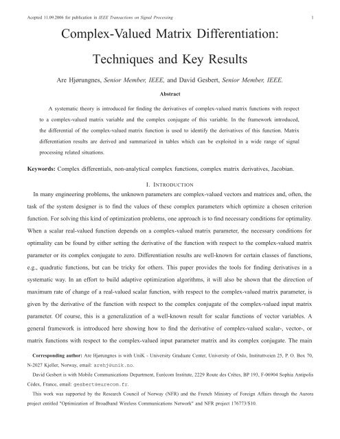
Acepted 11.09.2006 for publication in IEEE Transactions on Signal Processing 1Complex-Valued Matrix Differentiation:Techniques and Key ResultsAre Hjørungnes, Senior Member, IEEE, and David Gesbert, Senior Member, IEEE.AbstractA systematic theory is introduced for finding the derivatives of complex-valued matrix functions with respectto a complex-valued matrix variable and the complex conjugate of this variable. In the framework introduced,the differential of the complex-valued matrix function is used to identify the derivatives of this function. Matrixdifferentiation results are derived and summarized in tables which can be exploited in a wide range of signalprocessing related situations.Keywords: Complex differentials, non-analytical complex functions, complex matrix derivatives, Jacobian.I. INTRODUCTIONIn many engineering problems, the unknown parameters are complex-valued vectors and matrices and, often, thetask of the system designer is to find the values of these complex parameters which optimize a chosen criterionfunction. For solving this kind of optimization problems, one approach is to find necessary conditions for optimality.When a scalar real-valued function depends on a complex-valued matrix parameter, the necessary conditions foroptimality can be found by either setting the derivative of the function with respect to the complex-valued matrixparameter or its complex conjugate to zero. Differentiation results are well-known for certain classes of functions,e.g., quadratic functions, but can be tricky for others. This paper provides the tools for finding derivatives in asystematic way. In an effort to build adaptive optimization algorithms, it will also be shown that the direction ofmaximum rate of change of a real-valued scalar function, with respect to the complex-valued matrix parameter, isgiven by the derivative of the function with respect to the complex conjugate of the complex-valued input matrixparameter. Of course, this is a generalization of a well-known result for scalar functions of vector variables. Ageneral framework is introduced here showing how to find the derivative of complex-valued scalar-, vector-, ormatrix functions with respect to the complex-valued input parameter matrix and its complex conjugate. The mainCorresponding author: Are Hjørungnes is with UniK - University Graduate Center, University of Oslo, Instituttveien 25, P. O. Box 70,N-2027 Kjeller, Norway, email: arehj@unik.no.David Gesbert is with Mobile Communications Department, Eurécom Institute, 2229 Route des Crêtes, BP 193, F-06904 Sophia AntipolisCédex, France, email: gesbert@eurecom.fr.This work was supported by the Research Council of Norway (NFR) and the French Ministry of Foreign Affairs through the Auroraproject entitled "Optimization of Broadband Wireless Communications Network" and NFR project 176773/S10.

Acepted 11.09.2006 for publication in IEEE Transactions on Signal Processing 2TABLE ICLASSIFICATION OF FUNCTIONS.Function type Scalar variables z, z ∗ ∈ C Vector variables z, z ∗ ∈ C N ×1 Matrix variables Z, Z ∗ ∈ C N ×QScalar function f ∈ C f ( z, z ∗) f ( z, z ∗) f ( Z , Z ∗)f : C × C → C f : C N ×1 × C N ×1 → C f : C N ×Q × C N ×Q → CVector function f ∈ C M×1 f ( z, z ∗) f ( z, z ∗) f ( Z , Z ∗)f : C × C → C M×1 f : C N ×1 × C N ×1 → C M×1 f : C N ×Q × C N ×Q → C M×1Matrix function F ∈ C M×P F ( z, z ∗) F ( z, z ∗) F ( Z , Z ∗)F : C × C → C M×P F : C N ×1 × C N ×1 → C M×P F : C N ×Q × C N ×Q → C M×Pcontribution of this paper is to generalize the real-valued derivatives given in [1] to the complex-valued case. Thisis done by finding the derivatives by the so-called complex differentials of the functions. In this paper, it is assumedthat the functions are differentiable with respect to the complex-valued parameter matrix and its complex conjugate,and it will be seen that these two parameter matrices should be treated as independent when finding the derivatives,as is classical for scalar variables. The proposed theory is useful when solving numerous problems which involveoptimization when the unknown parameter is a complex-valued matrix.The problem at hand has been treated for real-valued matrix variables in [2], [1], [3], [4], [5]. Four additionalreferences that give a brief treatment of the case of real-valued scalar functions which depend complex-valuedvectors are Appendix B of [6], Appendix 2.B in [7], Subsection 2.3.10 of [8], and the article [9]. The article [10]serves as an introduction to this area for complex-valued scalar functions with complex-valued argument vectors.Results on complex differentiation theory is given in [11], [12] for differentiation with respect to complex-valuedscalars and vectors, however, the more general matrix case is not considered. In [13], the authors find derivativesof scalar functions with respect to complex-valued matrices, however, that paper could have been considerablysimplified if the proposed theory was utilized. Examples of problems where the unknown matrix is a complexvaluedmatrix are wide ranging including precoding of MIMO systems [14], linear equalization design [15], arraysignal processing [16] to only cite a few.Some of the most relevant applications to signal and communication problems are presented here, with key resultsbeing highlighted and other illustrative examples are listed in tables. For an extended version, see [17].The rest of this paper is organized as follows: In Section II, the complex differential is introduced, and based onthis differential, the definition of the derivatives of a complex-valued matrix function with respect to the complexvaluedmatrix argument and its complex conjugate is given in Section III. The key procedure showing how thederivatives can be found from the differential of a function is also presented in Section III. Section IV contains theimportant results of equivalent conditions for finding stationary points and in which direction the function has themaximum rate of change. In Section V, several key results are placed in tables and some results are derived forvarious cases with high relevance for signal processing and communication problems. Section VI contains someconclusions. Some of the proofs are given in the appendices.

Acepted 11.09.2006 for publication in IEEE Transactions on Signal Processing 3Notation: Scalar quantities (variables z or functions f) are denoted by lowercase symbols, vector quantities(variables z or functions f) are denoted by lowercase boldface symbols, and matrix quantities (variables Z orfunctions F ) are denoted by capital boldface symbols. The types of functions used throughout this paper areclassified in Table I. From the table, it is seen that all the functions depend on a complex variable and the complexconjugate of the same variable. Let j = √ −1, and and let the real Re{·} and imaginary Im{·} operators returnthe real and imaginary parts of the input matrix, respectively. If Z ∈ C N×Q is a complex-valued 1 matrix, thenZ =Re{Z} + j Im {Z}, and Z ∗ =Re{Z} −j Im {Z}, where Re {Z} ∈R N×Q , Im {Z} ∈R N×Q , and theoperator (·) ∗ denotes complex conjugate of the matrix it is applied to. The real and imaginary operators can beexpressed as Re {Z} = 1 2 (Z + Z∗ ) and Im {Z} = 1 2j (Z − Z∗ ).II. COMPLEX DIFFERENTIALSThe differential has the same size as the matrix it is applied to. The differential can be found component-wise,that is, (dZ) k,l= d (Z) k,l. A procedure that can often be used for finding the differentials of a complex-valuedmatrix function 2 F (Z 0 , Z 1 ) is to calculate the differenceF (Z 0 + dZ 0 , Z 1 + dZ 1 ) − F (Z 0 , Z 1 )=First-order(dZ 0 ,dZ 1 )+Higher-order(dZ 0 ,dZ 1 ), (1)where First-order(·, ·) returns the terms that depend on either dZ 0 or dZ 1 of the first order, and Higher-order(·, ·)returns the terms that depend on the higher order terms of dZ 0and dZ 1 . The differential is then given byFirst-order(·, ·), i.e., the first order term of F (Z 0 +dZ 0 , Z 1 +dZ 1 )−F (Z 0 , Z 1 ). As an example, let F (Z 0 , Z 1 )=Z 0 Z 1 . Then the difference in (1) can be developed and readily expressed as: F (Z 0 +dZ 0 , Z 1 +dZ 1 )−F (Z 0 , Z 1 )=Z 0 dZ 1 +(dZ 0 )Z 1 +(dZ 0 )(dZ 1 ). The differential of Z 0 Z 1 can then be identified as all the first-order terms oneither dZ 0 or dZ 1 as dZ 0 Z 1 = Z 0 dZ 1 +(dZ 0 )Z 1 .Let ⊗ and ⊙ denote the Kronecker and Hadamard product [18], respectively. Some of the most important rules oncomplex differentials are listed in Table II, assuming A, B, and a to be constants, and Z, Z 0 , and Z 1 to be complexvaluedmatrix variables. The vectorization operator vec(·) stacks the columns vectors of the argument matrix intoa long column vector in chronological order [18]. The differentiation rule of the reshaping operator reshape(·) inTable II is valid for any linear reshaping 3 operator reshape(·) of the matrix, and examples of such operators arethe transpose (·) T or vec(·). Some of the basic differential results in Table II can be derived by means of (1),and others can be derived by generalizing some of the results found in [1], [4] to the complex differential case.1 R and C are the sets of the real and complex numbers, respectively.2 The indexes are chosen to start with 0 everywhere in this article.3 The output of the reshape operator has the same number of elements as the input, but the shape of the output might be different, soreshape(·) performs a reshaping of its input argument.

Acepted 11.09.2006 for publication in IEEE Transactions on Signal Processing 6D Z ∗F (Z, Z ∗ )= ∂ vec(F (Z, Z∗ ))∂ vec T (Z ∗ . (7))This is a generalization of the real-valued matrix variable case treated in [1] to the complex-valued matrix variablecase. (6) and (7) show how the all the MPNQ partial derivatives of all the components of F with respect to allthe components of Z and Z ∗ are arranged when using the notation introduced in Definition 3.Key result: Finding the derivative of the complex-valued matrix function F with respect to the complex-valuedmatrices Z and Z ∗ can be achieved using the following three-step procedure:1) Compute the differential d vec(F ).2) Manipulate the expression into the form given (4).3) Read out the result using Table III.For less general function types, see Table I, a similar procedure can be used.Chain Rule: One big advantage of the way the derivative is defined in Definition 2 compared to other definitionsof the derivative of F (Z, Z ∗ ) is that the chain rule is valid. The chain rule is now formulated, and it might bevery useful for finding complicated derivatives.Theorem 1: Let (S 0 ,S 1 ) ⊆ C N×Q ×C N×Q , and let F : S 0 ×S 1 → C M×P be differentiable with respect to bothits first and second argument at an interior point (Z, Z ∗ ) in the set S 0 ×S 1 . Let T 0 ×T 1 ⊆ C M×P ×C M×P be suchthat (F (Z, Z ∗ ), F ∗ (Z, Z ∗ )) ∈ T 0 ×T 1 for all (Z, Z ∗ ) ∈ S 0 ×S 1 . Assume that G : T 0 ×T 1 → C R×S is differentiableat an interior point (F (Z, Z ∗ ), F ∗ (Z, Z ∗ )) ∈ T 0 × T 1 . Define the composite function H : S 0 × S 1 → C R×S byH (Z, Z ∗ ) G (F (Z, Z ∗ ), F ∗ (Z, Z ∗ )). The derivatives D Z H and D Z ∗H are obtained through:D Z H =(D F G)(D Z F )+(D F ∗G)(D Z F ∗ ) , (8)D Z ∗H =(D F G)(D Z ∗F )+(D F ∗G)(D Z ∗F ∗ ) . (9)Proof: From Definition 2, it follows that d vec(H) =d vec(G) =(D F G) d vec(F )+(D F ∗G) d vec(F ∗ ).The differentials of vec(F ) and vec(F ∗ ) are given by:d vec(F )=(D Z F ) d vec(Z)+(D Z ∗F ) d vec(Z ∗ ), (10)d vec(F ∗ )=(D Z F ∗ ) d vec(Z)+(D Z ∗F ∗ ) d vec(Z ∗ ). (11)By substituting the results from (10) and (11), into the expression for d vec(H), using the definition of the derivativeswith respect to Z and Z ∗ the theorem follows.IV. COMPLEX DERIVATIVES IN OPTIMIZATION THEORYIn this section, two useful theorems are presented that exploit the theory introduced earlier. Both theorems areimportant when solving practical optimization problems involving differentiation with respect to a complex-valuedmatrix. These results include conditions for finding stationary points for a real-valued scalar function dependent on

Acepted 11.09.2006 for publication in IEEE Transactions on Signal Processing 7complex-valued matrices and in which direction the same type of function has the minimum or maximum rate ofchange, which might be used in the steepest decent method.1) Stationary Points: The next theorem presents conditions for finding stationary points of f(Z, Z ∗ ) ∈ R.Theorem 2: Let f : C N×Q × C N×Q → R. A stationary point 5 of the function f(Z, Z ∗ )=g(X, Y ), whereg : R N×Q × R N×Q → R and Z = X + jY is then found by one of the following three equivalent conditions: 6D X g(X, Y )=0 1×NQ ∧ D Y g(X, Y )=0 1×NQ , (12)D Z f(Z, Z ∗ )=0 1×NQ , (13)orD Z ∗f(Z, Z ∗ )=0 1×NQ . (14)Proof: In optimization theory [1], a stationary point is a defined as point where the derivatives with respect toall the independent variables vanish. Since Re{Z} = X and Im{Z} = Y contain only independent variables, (12)gives a stationary point by definition. By using the chain rule in Theorem 1, on both sides of f(Z, Z ∗ )=g(X, Y )and taking the derivative with respect to X and Y , the following two equations are obtained:(D Z f)(D X Z)+(D Z ∗f)(D X Z ∗ )=D X g, (15)(D Z f)(D Y Z)+(D Z ∗f)(D Y Z ∗ )=D Y g. (16)From Table II, it follows that D X Z = D X Z ∗ = I NQ and D Y Z = −D Y Z ∗ = jI NQ . If these results are insertedinto (15) and (16), these two equations can be formulated into block matrix form in the following way:⎡ ⎤ ⎡ ⎤ ⎡ ⎤⎢⎣ D Xg ⎥ ⎢⎦ = ⎣ 1 1 ⎥ ⎢⎦ ⎣ D Zf ⎥⎦ . (17)D Y g j −j D Z ∗fThis equation is equivalent to the following matrix equation:⎡ ⎤ ⎡⎢⎣ D ZfD Z ∗f⎥⎦ =⎢⎣12− j 212j2⎤ ⎡ ⎤⎥ ⎢⎦ ⎣ D XgD Y g⎥⎦ . (18)Since D X g ∈ R 1×NQ and D Y g ∈ R 1×NQ , it is seen from (18), that (12), (13), and (14) are equivalent.5 Notice that a stationary point can be a local minimum, a local maximum, or a saddle point.6 In (12), the symbol ∧ means that both of the equations stated in (12) must be satisfied at the same time.

Acepted 11.09.2006 for publication in IEEE Transactions on Signal Processing 82) Direction of Extremal Rate of Change: The next theorem states how to find the maximum and minimumrate of change of f(Z, Z ∗ ) ∈ R.Theorem 3: Let f : C N×Q ×C N×Q → R. The directions where the function f have the maximum and minimumrate of change with respect to vec(Z) are given by [D Z ∗f(Z, Z ∗ )] T and − [D Z ∗f(Z, Z ∗ )] T , respectively.Proof: Since f ∈ R, df can be written in the following two ways df =(D Z f) d vec(Z)+(D Z ∗f) d vec(Z ∗ ),and df = df ∗ =(D Z f) ∗ d vec(Z ∗ )+(D Z ∗f) ∗ d vec(Z), where df = df ∗ since f ∈ R. Subtracting the two differentexpressions of df from each other and then applying Lemma 1, gives that D Z ∗f =(D Z f) ∗ and D Z f =(D Z ∗f) ∗ .From these results, it follows that: df = (D Z f) d vec(Z) +((D Z f) d vec(Z)) ∗ = 2Re{(D Z f) d vec(Z)} =2Re{(D Z ∗f) ∗ d vec(Z)}. Let a i ∈ C K×1 , where i ∈{0, 1}. ThenRe { 〈 ⎡ ⎤ ⎡ ⎤a H } ⎢ Re {a 0 } ⎥ ⎢0 a 1 = ⎣ ⎦ , ⎣ Re {a 〉1} ⎥⎦ , (19)Im {a 0 } Im {a 1 }where 〈·, ·〉 is the ordinary Euclidean inner product between real vectors in R 2K×1 . Using this on df gives〈 ⎡ ⎢ Re{(D Z ∗f) } ⎤ ⎡⎤T 〉df =2 ⎣ {Im (D Z ∗f) } ⎥ ⎢ Re {d vec(Z)} ⎥⎦ , ⎣ ⎦ . (20)T Im {d vec(Z)}Cauchy-Schwartz inequality gives that the maximum value of df occurs when d vec(Z) =α (D Z ∗f) T for α>0and from this, it follows that the minimum rate of change occurs when d vec(Z) =−β (D Z ∗f) T , for β>0.A. Derivative of f(Z, Z ∗ )V. DEVELOPMENT OF DERIVATIVE FORMULASFor functions of the type f (Z, Z ∗ ), it is common to arrange the partial derivatives∂∂z k,lf and∂∂z ∗ k,lf in analternative way [1] than in the expressions D Z f (Z, Z ∗ ) and D Z ∗f (Z, Z ∗ ). The notation for the alternative wayof organizing all the partial derivatives is∂∂Z f andelements of the matrix Z ∈ C N×Q are arranged as:⎡⎤∂∂∂z 0,0f ···∂z 0,Q−1f∂∂Z f = ⎢ ..⎥⎣⎦ ,∂∂∂z N −1,0f ···∂z N −1,Q−1f∂∗∂Zf. In this alternative way, the partial derivatives of the⎡∂∂Z ∗ f = ⎢⎣∂∂∂zf ···0,0∗ ∂zf0,Q−1 ∗.∂∂∂zf ···N ∗ −1,0∂zfN ∗ −1,Q−1.⎤⎥⎦ . (21)∂∂Z f and ∂∂Z f are called the ∗ gradient7 of f with respect to Z and Z ∗ , respectively. (21) generalizes to thecomplex case of one of the ways to define the derivative of real-valued scalar functions with respect to realmatrices in [1]. The way of arranging the partial derivatives in (21) is different than than the way given in (6) and(7). If df =vec T (A 0 )d vec(Z) +vec T (A 1 )d vec(Z ∗ )=Tr { A T 0 dZ + A T 1 dZ ∗} , where A i , Z ∈ C N×Q , then itcan be shown that∂∂Z f = A 0 and7 The following notation also exists [6], [13] for the gradient ∇ Z f ∂∂Z ∗ f.∂∂Z ∗ f = A 1, where the matrices A 0 and A 1 depend on Z and Z ∗ in general.

Acepted 11.09.2006 for publication in IEEE Transactions on Signal Processing 9f ( Z , Z ∗)TABLE IVDERIVATIVES OF FUNCTIONS OF THE TYPE f (Z, Z ∗ )Differential dfTr{Z } Tr {I N dZ } I N 0 N ×NTr{Z ∗ } Tr { I N dZ ∗} 0 N ×N I NTr{AZ} Tr {AdZ} A T 0 N ×Q{Tr{Z H A}Tr A T dZ ∗} 0 N ×Q A{() }Tr{ZA 0 Z T A 1 }Tr A 0 Z T A 1 + A T 0 Z T A T 1 dZA T 1 ZAT 0 + A 1ZA 0 0 N ×QTr{ZA 0 ZA 1 } Tr {(A 0 ZA 1 + A 1 ZA 0 ) dZ } A T 1 Z T A T 0 + AT 0 Z T A T 1 0 N ×Q{Tr{ZA 0 Z H A 1 }Tr A 0 Z H A 1 dZ + A T 0 Z T A T 1 dZ ∗} A T 1 Z ∗ A T 0 A 1 ZA 0Tr{ZA 0 Z ∗ A 1 } Tr { A 0 Z ∗ A 1 dZ + A 1 ZA 0 dZ ∗} A T 1 Z H A T 0 A T 0 Z T A T 1{}Tr{AZ −1 }− Tr Z −1 AZ −1 dZ−(Z ) T −1 ( ) ATZ T −10 N ×N{ }Tr{Z p }p Tr Z p−1 dZp(Z ) T p−10 N ×N{}()det(A 0 ZA 1 )det(A 0 ZA 1 )Tr A 1 (A 0 ZA 1 ) −1 A 0 dZdet(A 0 ZA 1 )A T 0 A T 1 Z T A T −10 AT1 0 N ×Qdet(ZZ T )2det(ZZ T )Tr{Z ( ) }T ZZ T −1 ( )dZ 2det(ZZ T ) ZZ T −1 Z 0N ×Qdet(ZZ ∗ )det(ZZ ∗ )Tr{Z ∗ (ZZ ∗ ) −1 dZ +(ZZ ∗ ) −1 Z dZ ∗} ( ) det(ZZ ∗ )(Z H Z T ) −1 Z H det(ZZ ∗ )Z T Z H Z T −1{( ) }det(ZZ H ) det(ZZ H )Tr Z H (ZZ H ) −1 dZ + Z T Z ∗ Z T −1 ( )dZ∗det(ZZ H )(Z ∗ Z T ) −1 Z ∗ det(ZZ H ) ZZ H −1 Z{ }det(Z p )p det p (Z)Tr Z −1 dZp det p (Z )(Z ) T −10 N ×N{}v H λ(Z )0 (dZ)u 0uv H =Tr 0 v H 0v ∗0 u 0v H dZ0 uT 00 u 0v H 0 N ×N0 u 0{}λ ∗ v T (Z )0 (dZ∗ )u ∗ 0u ∗v T =Tr 0 vT 00 u∗ 0v T dZ ∗ v0 0 u H 0N ×N0 u∗ 0v T 0 u∗ 0∂∂Z f∂∂Z ∗ fThis result is included in Table III. The size of∂∂Z f and∂∂Z ∗ f is N × Q, while the size of D Zf (Z, Z ∗ ) andD Z ∗f (Z, Z ∗ ) is 1×NQ, so these two ways of organizing the partial derivatives are different. It can be shown, thatD Z f (Z, Z ∗ )=vec T ( ∂∂Z f (Z, Z∗ ) ) , and D Z ∗f (Z, Z ∗ )=vec T ( ∂∂Z f (Z, ∗ Z∗ ) ) . The steepest decent method canbe formulated as Z k+1 = Z k + μ ∂∂Z f(Z k, Z ∗ ∗ k ). The differentials of the simple eigenvalue λ and its complexconjugate λ ∗ at Z 0 are derived in [1] and they are included in Table IV. One key example of derivatives is developedin the text below, while others useful results are stated in Table IV.1) Determinant Related Problems: Objective functions that depend on the determinant appear in several partsof signal processing related problems, e.g., in the capacity of wireless multiple-input multiple-output (MIMO)communication systems [15], and in an upper bound for the pair-wise error probability (PEP) [14].Let f : C N×Q × C Q×N → C be f(Z, Z ∗ )=det(P + ZZ H ), where P ∈ C N×N is independent of Z andZ ∗ . df is found by the rules in Table II as df = det(P + ZZ H )Tr { (P + ZZ H ) −1 d(ZZ H ) } =det(P +{ZZ H )Tr Z H ( P + ZZ H) −1dZ + Z T (P + ZZ H ) −T dZ ∗} . From this, the derivatives with respect to Z andZ ∗ of det ( P + ZZ H) can be found, but since these results are relatively long, they are not included in Table IV.B. Derivative of F (Z, Z ∗ )1) Kronecker Product Related Problems: An objective functions which depends on the Kronecker product ofthe unknown complex-valued matrix is the PEP found in [14]. Let K N,Q denote the commutation 8 matrix [1]. LetF : C N0×Q0 × C N1×Q1 → C N0N1×Q0Q1 be given by F (Z 0 , Z 1 )=Z 0 ⊗ Z 1 , where Z i ∈ C Ni×Qi . The differentialof this function follows from Table II: dF =(dZ 0 ) ⊗ Z 1 + Z 0 ⊗ dZ 1 . Applying the vec(·) operator to dF yields:8 The commutation matrix K k,l is the unique kl × kl permutation matrix satisfying K k,l vec (A) =vec ( A ) T for all matrices A ∈ C k×l .

Acepted 11.09.2006 for publication in IEEE Transactions on Signal Processing 10TABLE VDERIVATIVES OF FUNCTIONS OF THE TYPE F (Z, Z ∗ )F ( Z , Z ∗) Differential d vec(F ) D Z F ( Z, Z ∗) D Z ∗ F ( Z, Z ∗)Z I NQ d vec(Z ) I NQ 0 NQ×NQZ T K N,Q d vec(Z) K N,Q 0 NQ×NQZ ∗ I NQ d vec(Z ∗ ) 0 NQ×NQ I NQZ H K N,Q d vec(Z ∗ ) 0 NQ×NQ K N,Q())ZZ T I N 2 + K N,N (Z ⊗ I N ) d vec(Z)(I N 2 + K N,N (Z ⊗ I N ) 0 N 2 ×NQZ T Z(I Q 2 + K Q,Q)(I Q ⊗ Z T ) d vec(Z )(I Q 2 + K Q,Q)(I Q ⊗ Z T )0 Q 2 ×NQZZ H (Z∗ )⊗ I N d vec(Z )+K N,N (Z ⊗ I N ) d vec(Z ∗ ) Z ∗ ⊗ I N K N,N (Z ⊗ I N )Z −1(− (Z T ) −1 ⊗ Z −1) d vec(Z ) −(Z T ) −1 ⊗ Z −1 0 N 2 ×N 2Z p∑ p ((Z T ) p−i ⊗ Z i−1) p∑ (d vec(Z )(Z T ) p−i ⊗ Z i−1) 0 N 2 ×N 2i=1i=1Z ⊗ Z (A(Z )+B(Z ))d vec(Z ) A(Z )+B(Z ) 0 N 2 Q 2 ×NQZ ⊗ Z ∗ A(Z ∗ )d vec(Z )+B(Z)d vec(Z ∗ ) A(Z ∗ ) B(Z)Z ∗ ⊗ Z ∗ (A(Z ∗ )+B(Z ∗ ))d vec(Z ∗ ) 0 N 2 Q 2 ×NQA(Z ∗ )+B(Z ∗ )Z ⊙ Z 2 diag(vec(Z ))d vec(Z ) 2 diag(vec(Z )) 0 NQ×NQZ ⊙ Z ∗ diag(vec(Z ∗ ))d vec(Z )+diag(vec(Z))d vec(Z ∗ ) diag(vec(Z ∗ )) diag(vec(Z ))Z ∗ ⊙ Z ∗ 2diag(vec(Z ∗ ))d vec(Z ∗ ) 0 NQ×NQ 2diag(vec(Z ∗ ))d vec(F )=vec((dZ 0 ) ⊗ Z 1 )+vec(Z 0 ⊗ dZ 1 ). From Theorem 3.10 in [1], it follows thatvec ((dZ 0 ) ⊗ Z 1 )=(I Q0 ⊗ K Q1,N 0⊗ I N1 )[(d vec(Z 0 )) ⊗ vec(Z 1 )]=(I Q0 ⊗ K Q1,N 0⊗ I N1 )[I N0Q 0⊗ vec(Z 1 )] d vec(Z 0 ), (22)and in a similar way it follows that: vec (Z 0 ⊗ dZ 1 ) = (I Q0 ⊗ K Q1,N 0⊗ I N1 )[vec(Z 0 ) ⊗ I N1Q 1] d vec(Z 1 ).Inserting the last two results into d vec(F ) gives:d vec(F )=(I Q0 ⊗ K Q1,N 0⊗ I N1 )[I N0Q 0⊗ vec(Z 1 )] d vec(Z 0 )+(I Q0 ⊗ K Q1,N 0⊗ I N1 )[vec(Z 0 ) ⊗ I N1Q 1] d vec(Z 1 ). (23)Define the matrices A(Z 1 ) and B(Z 0 ) by A(Z 1 ) (I Q0 ⊗ K Q1,N 0⊗ I N1 )[I N0Q 0⊗ vec(Z 1 )], and B(Z 0 )=(I Q0 ⊗ K Q1,N 0⊗ I N1 )[vec(Z 0 ) ⊗ I N1Q 1]. It is then possible to rewrite the differential of F (Z 0 , Z 1 )=Z 0 ⊗ Z 1as d vec(F )=A(Z 1 )d vec(Z 0 )+B(Z 0 )d vec(Z 1 ). From d vec(F ), the differentials and derivatives of Z ⊗ Z,Z ⊗ Z ∗ , and Z ∗ ⊗ Z ∗ can be derived and these results are included in Table V. In the table, diag(·) returns thesquare diagonal matrix with the input column vector elements on the main diagonal [19] and zeros elsewhere.2) Moore-Penrose Inverse Related Problems: In pseudo-inverse matrix based receiver design, the Moore-Penrose inverse might appear [15]. This is applicable for MIMO, CDMA, and OFDM systems.Let F : C N×Q × C N×Q → C Q×N be given by F (Z, Z ∗ )=Z + , where Z ∈ C N×Q . The reason for includingboth variables Z and Z ∗ in this function definition is that the differential of Z + , see Proposition 1, depends onboth dZ and dZ ∗ . Using the vec(·) operator on the differential of the Moore-Penrose inverse in Table II, in additionto Lemma 4.3.1 in [18] and the definition of the commutation matrix, result in:[ (Z+d vec(F )=− ) ] [(T ⊗ Z+d vec(Z)+ I N − ( Z +) ) T ZT⊗ Z + ( Z +) ] HK N,Q d vec(Z ∗ )

Acepted 11.09.2006 for publication in IEEE Transactions on Signal Processing 11This leads to D Z ∗F =+[ (Z+ ) T ( Z +) ∗ ⊗(IQ − Z + Z )] K N,Q d vec(Z ∗ ). (24){[(I N − ( Z +) T ZT ) ⊗ Z + ( Z +) H ] +[ (Z+ ) T (Z+ ) ∗ ⊗(IQ − Z + Z )]} K N,Q andD Z F = −[ (Z+ ) T ⊗ Z+ ] .IfZ is invertible, then the derivative of Z + = Z −1 with respect to Z ∗ is equal to thezero matrix and the derivative of Z + = Z −1 with respect to Z can be found from Table V.VI. CONCLUSIONSAn introduction is given to a set of very powerful tools that can be used to systematically find the derivative ofcomplex-valued matrix functions that are dependent on complex-valued matrices. The key idea is to go through thecomplex differential of the function and to treat the differential of the complex variable and its complex conjugateas independent. This general framework can be used in many optimization problems that depend on complexparameters. Many results are given in tabular form.APPENDIX IPROOF OF PROPOSITION 1Proof: (2) leads to dZ + = dZ + ZZ + =(dZ + Z)Z + + Z + ZdZ + .IfZdZ + is found from dZZ + =(dZ)Z + + ZdZ + , and inserted in the expression for dZ + , then it is found that:dZ + =(dZ + Z)Z + + Z + (dZZ + − (dZ)Z + )=(dZ + Z)Z + + Z + dZZ + − Z + (dZ)Z + . (25)It is seen from (25), that it remains to express dZ + Z and dZZ + in terms of dZ and dZ ∗ . Firstly, dZ + Z ishandled:dZ + Z = dZ + ZZ + Z =(dZ + Z)Z + Z + Z + Z(dZ + Z)=(Z + Z(dZ + Z)) H + Z + Z(dZ + Z). (26)The expression Z(dZ + Z) can be found from dZ = dZZ + Z =(dZ)Z + Z + Z(dZ + Z), and it is given byZ(dZ + Z)=dZ − (dZ)Z + Z =(dZ)(I Q − Z + Z). If this expression is inserted into (26), it is found that:dZ + Z =(Z + (dZ)(I Q −Z + Z)) H +Z + (dZ)(I Q −Z + Z)=(I Q −Z + Z) ( dZ H) (Z + ) H +Z + (dZ)(I Q −Z + Z).Secondly, it can be shown in a similar manner that: dZZ + =(I N −ZZ + )(dZ)Z + +(Z + ) H ( dZ H) (I N −ZZ + ).If the expressions for dZ + Z and dZZ + are inserted into (25), (3) is obtained.APPENDIX IIPROOF OF LEMMA 1Proof: Let A i ∈ C M×NQ be an arbitrary complex-valued function of Z ∈ C N×Q and Z ∗ ∈ C N×Q .From Table II, it follows that d vec(Z) =d vec(Re {Z}) +jd vec(Im {Z}) and d vec(Z ∗ )=d vec(Re {Z}) −jd vec(Im {Z}). If these two expressions are substituted into A 0 d vec(Z)+A 1 d vec(Z ∗ )=0 M×1 , then it followsthat A 0 (d vec(Re {Z})+jd vec(Im {Z})) + A 1 (d vec(Re {Z}) − jd vec(Im {Z})) = 0 M×1 . The last expressionis equivalent to: (A 0 + A 1 )d vec(Re {Z})+j(A 0 − A 1 )d vec(Im {Z}) =0 M×1 . Since the differentials d Re {Z}

Acepted 11.09.2006 for publication in IEEE Transactions on Signal Processing 12and d Im {Z} are independent, so are d vec(Re {Z}) and d vec(Im {Z}). Therefore, A 0 + A 1 = 0 M×NQ andA 0 − A 1 = 0 M×NQ . And from this it follows that A 0 = A 1 = 0 M×NQ .REFERENCES[1] J. R. Magnus and H. Neudecker, Matrix Differential Calculus with Application in Statistics and Econometrics. Essex, England: JohnWiley & Sons, Inc., 1988.[2] J. W. Brewer, “Kronecker products and matrix calculus in system theory,” IEEE Trans. Circuits, Syst., vol. CAS-25, no. 9, pp. 772–781,Sept. 1978.[3] D. A. Harville, Matrix Algebra from a Statistician’s Perspective. Springer-Verlag, 1997, corrected second printing, 1999.[4] T. P. Minka. (December 28, 2000) Old and new matrix algebra useful for statistics. [Online]. Available: http://research.microsoft.com/~minka/papers/matrix/[5] K. Kreutz-Delgado, “Real vector derivatives and gradients,” Dept. of Electrical and Computer Engineering, UC San Diego, Tech. Rep.Course Lecture Supplement No. ECE275A, December 5. 2005, http://dsp.ucsd.edu/~kreutz/PEI05.html.[6] S. Haykin, Adaptive Filter Theory, 4th ed. Englewood Cliffs, New Jersey, USA: Prentice Hall, 2002.[7] A. H. Sayed, Fundamentals of Adaptive Filtering. IEEE Computer Society Press, 2003.[8] M. H. Hayes, Statistical Digital Signal Processing and Modeling. John Wiley & Sons, Inc., 1996.[9] A. van den Bos, “Complex gradient and Hessian,” Proc. IEE Vision, Image and Signal Process., vol. 141, no. 6, pp. 380–383, Dec.1994.[10] D. H. Brandwood, “A complex gradient operator and its application in adaptive array theory,” IEE Proc., Parts F and H, vol. 130,no. 1, pp. 11–16, Feb. 1983.[11] M. Brookes. Matrix reference manual. [Online]. Available: http://www.ee.ic.ac.uk/hp/staff/dmb/matrix/intro.html[12] K. Kreutz-Delgado, “The complex gradient operator and the CR-calculus,” Dept. of Electrical and Computer Engineering, UC San Diego,Tech. Rep. Course Lecture Supplement No. ECE275A, Sept.-Dec. 2005, http://dsp.ucsd.edu/~kreutz/PEI05.html.[13] D. P. Palomar and S. Verdú, “Gradient of mutual information in linear vector Gaussian channels,” IEEE Trans. Inform. Theory, vol. 52,no. 1, pp. 141–154, Jan. 2006.[14] G. Jöngren, M. Skoglund, and B. Ottersten, “Combining beamforming and orthogonal space-time block coding,” IEEE Trans. Inform.Theory, vol. 48, no. 3, pp. 611–627, Mar. 2002.[15] D. Gesbert, M. Shafi, D. Shiu, P. J. Smith, and A. Naguib, “From theory to practice: An overview of MIMO space-time coded wirelesssystems,” IEEE J. Select. Areas Commun., vol. 21, no. 3, pp. 281–302, Apr. 2003.[16] D. H. Jonhson and D. A. Dudgeon, Array Signal Processing: Concepts and Techniques. Prentice-Hall, Inc., 1993.[17] A. Hjørungnes and D. Gesbert. Introduction to complex-valued matrix differentiation. [Online]. Available: http://www.unik.no/personer/arehj/publications/matrixdiff.pdf[18] R. A. Horn and C. R. Johnson, Topics in Matrix Analysis. Cambridge University Press Cambridge, UK, 1991, reprinted 1999.[19] ——, Matrix Analysis. Cambridge University Press Cambridge, UK, 1985, reprinted 1999.