- Page 2:
Quantum Gravitation
- Page 8:
Prof. Dr. Herbert W. HamberUniversi
- Page 16:
viiiPrefaceenough conspiracies migh
- Page 20:
xPrefacetal energy of a quantum gra
- Page 24:
xiiPrefaceA final section touches o
- Page 30:
Contents1 Continuum Formulation ...
- Page 34:
Contentsxvii7 Analytical Lattice Ex
- Page 38:
2 1 Continuum Formulation+c∂ ν h
- Page 48:
1.3 Wave Equation 7Fig. 1.1 Lowest
- Page 52:
1.3 Wave Equation 9withs μν = 1 d
- Page 56:
1.4 Feynman Rules 11One can exploit
- Page 60:
1.4 Feynman Rules 13and the gravito
- Page 64:
1.4 Feynman Rules 15where the p 1 ,
- Page 68:
1.5 One-Loop Divergences 17D = 2 +(
- Page 72:
1.5 One-Loop Divergences 19R 2 =
- Page 76:
1.6 Gravity in d Dimensions 211.6 G
- Page 80:
1.6 Gravity in d Dimensions 23∇ 2
- Page 84:
1.7 Higher Derivative Terms 25case,
- Page 88:
1.7 Higher Derivative Terms 27theor
- Page 92:
1.7 Higher Derivative Terms 29∫I
- Page 96:
1.7 Higher Derivative Terms 31trln
- Page 100:
1.8 Supersymmetry 33treated perturb
- Page 104:
1.8 Supersymmetry 35and Σ’s has
- Page 108:
1.9 Supergravity 37δA μ = −2g
- Page 114:
40 1 Continuum Formulationβ 0 =
- Page 120:
1.10 String Theory 43Solutions to t
- Page 124:
1.10 String Theory 45and for the op
- Page 128:
1.10 String Theory 47with [dg ab ]
- Page 132:
1.11 Supersymmetric Strings 49One w
- Page 138:
52 1 Continuum Formulationallowed o
- Page 142:
54 1 Continuum Formulationdate no c
- Page 146:
56 2 Feynman Path Integral Formulat
- Page 150:
58 2 Feynman Path Integral Formulat
- Page 154:
60 2 Feynman Path Integral Formulat
- Page 158:
62 2 Feynman Path Integral Formulat
- Page 162:
64 2 Feynman Path Integral Formulat
- Page 166:
66 2 Feynman Path Integral Formulat
- Page 170:
68 3 Gravity in 2 + ε DimensionsLa
- Page 174:
70 3 Gravity in 2 + ε Dimensions
- Page 178:
72 3 Gravity in 2 + ε DimensionsΛ
- Page 182:
74 3 Gravity in 2 + ε Dimensionsg(
- Page 186:
76 3 Gravity in 2 + ε DimensionsFo
- Page 190:
78 3 Gravity in 2 + ε DimensionsTh
- Page 194:
80 3 Gravity in 2 + ε Dimensions
- Page 198:
82 3 Gravity in 2 + ε Dimensionsβ
- Page 202:
84 3 Gravity in 2 + ε DimensionsIn
- Page 206:
86 3 Gravity in 2 + ε Dimensionsan
- Page 210:
88 3 Gravity in 2 + ε Dimensions(
- Page 214:
90 3 Gravity in 2 + ε DimensionsTh
- Page 218:
92 3 Gravity in 2 + ε Dimensionsor
- Page 222:
94 3 Gravity in 2 + ε Dimensionsno
- Page 226:
96 3 Gravity in 2 + ε Dimensionsβ
- Page 230:
98 3 Gravity in 2 + ε DimensionsNo
- Page 234:
100 3 Gravity in 2 + ε Dimensions(
- Page 240:
Chapter 4Hamiltonian and Wheeler-De
- Page 244:
4.2 First Order Formulation 105ṗ
- Page 248:
4.3 Arnowitt-Deser-Misner (ADM) For
- Page 252:
4.3 Arnowitt-Deser-Misner (ADM) For
- Page 256:
4.5 Intrinsic and Extrinsic Curvatu
- Page 260:
4.6 Matter Source Terms 113One stil
- Page 264:
4.8 Semiclassical Expansion of the
- Page 268:
4.9 Connection with the Feynman Pat
- Page 272:
4.10 Minisuperspace 119is the inver
- Page 276:
4.10 Minisuperspace 121H = p a ȧ +
- Page 280:
4.11 Solution of Simple Minisupersp
- Page 284:
4.11 Solution of Simple Minisupersp
- Page 288:
4.12 Quantum Hamiltonian for Gauge
- Page 292:
4.13 Lattice Regularized Hamiltonia
- Page 296:
4.13 Lattice Regularized Hamiltonia
- Page 300:
4.13 Lattice Regularized Hamiltonia
- Page 304:
4.14 Lattice Hamiltonian for Quantu
- Page 308:
4.14 Lattice Hamiltonian for Quantu
- Page 312:
4.14 Lattice Hamiltonian for Quantu
- Page 316:
Chapter 5Semiclassical Gravity5.1 C
- Page 320:
5.1 Cosmological Wavefunctions 143P
- Page 324:
5.1 Cosmological Wavefunctions 145w
- Page 328:
5.2 Semiclassical Expansion 147with
- Page 332:
5.2 Semiclassical Expansion 149logP
- Page 336:
5.2 Semiclassical Expansion 151∫
- Page 340:
5.3 Pair Creation in Constant Elect
- Page 344:
5.4 Black Hole Particle Emission 15
- Page 348:
5.4 Black Hole Particle Emission 15
- Page 352:
5.5 Method of In and Out Vacua 159[
- Page 356:
5.5 Method of In and Out Vacua 161o
- Page 360:
5.6 Complex Periodic Time 1635.6 Co
- Page 364:
5.6 Complex Periodic Time 165with
- Page 368:
5.8 Quantum Gravity Corrections 167
- Page 372:
Chapter 6Lattice Regularized Quantu
- Page 376:
6.3 Volumes and Angles 171Fig. 6.2
- Page 380:
6.4 Rotations, Parallel Transports
- Page 384:
6.4 Rotations, Parallel Transports
- Page 388:
6.4 Rotations, Parallel Transports
- Page 392:
6.5 Invariant Lattice Action 1796.5
- Page 396:
6.5 Invariant Lattice Action 181The
- Page 400:
6.5 Invariant Lattice Action 183whe
- Page 404:
6.6 Lattice Diffeomorphism Invarian
- Page 408:
6.7 Lattice Bianchi Identities 187F
- Page 412:
6.8 Gravitational Wilson Loop 189wh
- Page 416:
6.9 Lattice Regularized Path Integr
- Page 420:
6.9 Lattice Regularized Path Integr
- Page 424:
6.10 An Elementary Example 195∫Z
- Page 428:
6.10 An Elementary Example 197where
- Page 432:
6.11 Lattice Higher Derivative Term
- Page 436:
6.11 Lattice Higher Derivative Term
- Page 440: 6.12 Scalar Matter Fields 203if and
- Page 444: 6.12 Scalar Matter Fields 205A ij i
- Page 448: 6.12 Scalar Matter Fields 207define
- Page 452: 6.13 Invariance Properties of the S
- Page 456: 6.14 Lattice Fermions, Tetrads and
- Page 460: 6.15 Gauge Fields 2136.15 Gauge Fie
- Page 464: 6.16 Lattice Gravitino 215and invol
- Page 468: 6.17 Alternate Discrete Formulation
- Page 472: 6.17 Alternate Discrete Formulation
- Page 476: 6.18 Lattice Invariance versus Cont
- Page 480: 6.18 Lattice Invariance versus Cont
- Page 484: Chapter 7Analytical Lattice Expansi
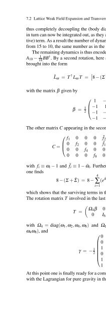
- Page 488: 7.2 Lattice Weak Field Expansion an
- Page 494: 230 7 Analytical Lattice Expansion
- Page 498: 232 7 Analytical Lattice Expansion
- Page 502: 234 7 Analytical Lattice Expansion
- Page 506: 236 7 Analytical Lattice Expansion
- Page 510: 238 7 Analytical Lattice Expansion
- Page 514: 240 7 Analytical Lattice Expansion
- Page 518: 242 7 Analytical Lattice Expansion
- Page 522: 244 7 Analytical Lattice Expansion
- Page 526: 246 7 Analytical Lattice Expansion
- Page 530: 248 7 Analytical Lattice Expansion
- Page 534: 250 7 Analytical Lattice Expansion
- Page 538: 252 7 Analytical Lattice Expansion
- Page 542:
254 7 Analytical Lattice Expansion
- Page 546:
256 7 Analytical Lattice Expansion
- Page 550:
258 7 Analytical Lattice Expansion
- Page 554:
260 7 Analytical Lattice Expansion
- Page 558:
262 7 Analytical Lattice Expansion
- Page 562:
264 7 Analytical Lattice Expansion
- Page 566:
266 7 Analytical Lattice Expansion
- Page 570:
268 7 Analytical Lattice Expansion
- Page 574:
270 7 Analytical Lattice Expansion
- Page 580:
Chapter 8Numerical Studies8.1 Nonpe
- Page 584:
8.2 Observables, Phase Structure an
- Page 588:
8.3 Invariant Local Gravitational A
- Page 592:
8.4 Invariant Correlations at Fixed
- Page 596:
8.5 Wilson Lines and Static Potenti
- Page 600:
8.5 Wilson Lines and Static Potenti
- Page 604:
8.7 Physical and Unphysical Phases
- Page 608:
8.7 Physical and Unphysical Phases
- Page 612:
8.7 Physical and Unphysical Phases
- Page 616:
8.8 Numerical Determination of the
- Page 620:
8.8 Numerical Determination of the
- Page 624:
8.9 Renormalization Group and Latti
- Page 628:
8.9 Renormalization Group and Latti
- Page 632:
8.9 Renormalization Group and Latti
- Page 636:
8.10 Curvature Scales 301for gravit
- Page 640:
8.11 Gravitational Condensate 303wh
- Page 646:
306 9 Scale Dependent Gravitational
- Page 650:
308 9 Scale Dependent Gravitational
- Page 654:
310 9 Scale Dependent Gravitational
- Page 658:
312 9 Scale Dependent Gravitational
- Page 662:
314 9 Scale Dependent Gravitational
- Page 666:
316 9 Scale Dependent Gravitational
- Page 670:
318 9 Scale Dependent Gravitational
- Page 674:
320 9 Scale Dependent Gravitational
- Page 678:
322 9 Scale Dependent Gravitational
- Page 684:
ReferencesAbbott, L., 1982, Introdu
- Page 688:
References 327Das, A., 1977, Phys.
- Page 692:
References 329Hartle, J. B., 1985,
- Page 696:
References 331Parisi, G., 1979, Phy
- Page 700:
References 333Williams, R. M., 1986
- Page 706:
336 IndexCauchy problem, 103, 107ce
- Page 710:
338 Indexgravitational exponent ν,
- Page 714:
340 Indexperfect fluid, 311periodic
- Page 718:
342 Indexthermodynamic analogy, 158


![arXiv:1001.0993v1 [hep-ph] 6 Jan 2010](https://img.yumpu.com/51282177/1/190x245/arxiv10010993v1-hep-ph-6-jan-2010.jpg?quality=85)


![arXiv:1008.3907v2 [astro-ph.CO] 1 Nov 2011](https://img.yumpu.com/48909562/1/190x245/arxiv10083907v2-astro-phco-1-nov-2011.jpg?quality=85)


![arXiv:1002.4928v1 [gr-qc] 26 Feb 2010](https://img.yumpu.com/41209516/1/190x245/arxiv10024928v1-gr-qc-26-feb-2010.jpg?quality=85)
![arXiv:1206.2653v1 [astro-ph.CO] 12 Jun 2012](https://img.yumpu.com/39510078/1/190x245/arxiv12062653v1-astro-phco-12-jun-2012.jpg?quality=85)
