Contact Geometry - Mathematisches Institut der Universität zu Köln
Contact Geometry - Mathematisches Institut der Universität zu Köln
Contact Geometry - Mathematisches Institut der Universität zu Köln

You also want an ePaper? Increase the reach of your titles
YUMPU automatically turns print PDFs into web optimized ePapers that Google loves.
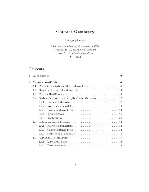
Contents<br />
<strong>Contact</strong> <strong>Geometry</strong><br />
Hansjörg Geiges<br />
<strong>Mathematisches</strong> <strong>Institut</strong>, <strong>Universität</strong> <strong>zu</strong> <strong>Köln</strong>,<br />
Weyertal 86–90, 50931 <strong>Köln</strong>, Germany<br />
E-mail: geiges@math.uni-koeln.de<br />
April 2004<br />
1 Introduction 3<br />
2 <strong>Contact</strong> manifolds 4<br />
2.1 <strong>Contact</strong> manifolds and their submanifolds . . . . . . . . . . . . . . 6<br />
2.2 Gray stability and the Moser trick . . . . . . . . . . . . . . . . . . 13<br />
2.3 <strong>Contact</strong> Hamiltonians . . . . . . . . . . . . . . . . . . . . . . . . . 16<br />
2.4 Darboux’s theorem and neighbourhood theorems . . . . . . . . . . 17<br />
2.4.1 Darboux’s theorem . . . . . . . . . . . . . . . . . . . . . . . 17<br />
2.4.2 Isotropic submanifolds . . . . . . . . . . . . . . . . . . . . . 19<br />
2.4.3 <strong>Contact</strong> submanifolds . . . . . . . . . . . . . . . . . . . . . 24<br />
2.4.4 Hypersurfaces . . . . . . . . . . . . . . . . . . . . . . . . . . 26<br />
2.4.5 Applications . . . . . . . . . . . . . . . . . . . . . . . . . . 30<br />
2.5 Isotopy extension theorems . . . . . . . . . . . . . . . . . . . . . . 32<br />
2.5.1 Isotropic submanifolds . . . . . . . . . . . . . . . . . . . . . 32<br />
2.5.2 <strong>Contact</strong> submanifolds . . . . . . . . . . . . . . . . . . . . . 34<br />
2.5.3 Surfaces in 3–manifolds . . . . . . . . . . . . . . . . . . . . 36<br />
2.6 Approximation theorems . . . . . . . . . . . . . . . . . . . . . . . . 37<br />
2.6.1 Legendrian knots . . . . . . . . . . . . . . . . . . . . . . . . 38<br />
2.6.2 Transverse knots . . . . . . . . . . . . . . . . . . . . . . . . 42<br />
1
3 <strong>Contact</strong> structures on 3–manifolds 43<br />
3.1 An invariant of transverse knots . . . . . . . . . . . . . . . . . . . . 45<br />
3.2 Martinet’s construction . . . . . . . . . . . . . . . . . . . . . . . . 46<br />
3.3 2–plane fields on 3–manifolds . . . . . . . . . . . . . . . . . . . . . 50<br />
3.3.1 Hopf’s Umkehrhomomorphismus . . . . . . . . . . . . . . . 53<br />
3.3.2 Representing homology classes by submanifolds . . . . . . . 54<br />
3.3.3 Framed cobordisms . . . . . . . . . . . . . . . . . . . . . . . 56<br />
3.3.4 Definition of the obstruction classes . . . . . . . . . . . . . 57<br />
3.4 Let’s Twist Again . . . . . . . . . . . . . . . . . . . . . . . . . . . 59<br />
3.5 Other existence proofs . . . . . . . . . . . . . . . . . . . . . . . . . 64<br />
3.5.1 Open books . . . . . . . . . . . . . . . . . . . . . . . . . . . 64<br />
3.5.2 Branched covers . . . . . . . . . . . . . . . . . . . . . . . . 66<br />
3.5.3 . . . and more . . . . . . . . . . . . . . . . . . . . . . . . . 67<br />
3.6 Tight and overtwisted . . . . . . . . . . . . . . . . . . . . . . . . . 67<br />
3.7 Classification results . . . . . . . . . . . . . . . . . . . . . . . . . . 73<br />
4 A guide to the literature 75<br />
4.1 Dimension 3 . . . . . . . . . . . . . . . . . . . . . . . . . . . . . . . 76<br />
4.2 Higher dimensions . . . . . . . . . . . . . . . . . . . . . . . . . . . 76<br />
4.3 Symplectic fillings . . . . . . . . . . . . . . . . . . . . . . . . . . . 77<br />
4.4 Dynamics of the Reeb vector field . . . . . . . . . . . . . . . . . . . 77<br />
2
1 Introduction<br />
Over the past two decades, contact geometry has un<strong>der</strong>gone a veritable meta-<br />
morphosis: once the ugly duckling known as ‘the odd-dimensional analogue of<br />
symplectic geometry’, it has now evolved into a proud field of study in its own<br />
right. As is typical for a period of rapid development in an area of mathematics,<br />
there are a fair number of folklore results that every mathematician working in<br />
the area knows, but no references that make these results accessible to the novice.<br />
I therefore take the present article as an opportunity to take stock of some of that<br />
folklore.<br />
There are many excellent surveys covering specific aspects of contact geometry<br />
(e.g. classification questions in dimension 3, dynamics of the Reeb vector field,<br />
various notions of symplectic fillability, transverse and Legendrian knots and<br />
links). All these topics deserve to be included in a comprehensive survey, but<br />
an attempt to do so here would have left this article in the ‘to appear’ limbo for<br />
much too long.<br />
Thus, instead of adding yet another survey, my plan here is to cover in detail<br />
some of the more fundamental differential topological aspects of contact geometry.<br />
In doing so, I have not tried to hide my own idiosyncrasies and preoccupations.<br />
Owing to a relatively leisurely pace and constraints of the present format, I<br />
have not been able to cover quite as much material as I should have wished.<br />
Nonetheless, I hope that the rea<strong>der</strong> of the present handbook chapter will be<br />
better prepared to study some of the surveys I alluded to – a guide to these<br />
surveys will be provided – and from there to move on to the original literature.<br />
A book chapter with comparable aims is Chapter 8 in [1]. It seemed opportune<br />
to be brief on topics that are covered extensively there, even if it is done at the<br />
cost of leaving out some essential issues. I hope to return to the material of the<br />
present chapter in a yet to be written more comprehensive monograph.<br />
Acknowledgements. I am grateful to Fan Ding, Jesús Gonzalo and Fe<strong>der</strong>ica<br />
Pasquotto for their attentive reading of the original manuscript. I also thank<br />
John Etnyre and Stephan Schönenberger for allowing me to use a couple of their<br />
figures (viz., Figures 2 and 1 of the present text, respectively).<br />
3
2 <strong>Contact</strong> manifolds<br />
Let M be a differential manifold and ξ ⊂ TM a field of hyperplanes on M. Locally<br />
such a hyperplane field can always be written as the kernel of a non-vanishing<br />
1–form α. One way to see this is to choose an auxiliary Riemannian metric g on<br />
M and then to define α = g(X, .), where X is a local non-zero section of the line<br />
bundle ξ ⊥ (the orthogonal complement of ξ in TM). We see that the existence<br />
of a globally defined 1–form α with ξ = kerα is equivalent to the orientability<br />
(hence triviality) of ξ ⊥ , i.e. the coorientability of ξ. Except for an example below,<br />
I shall always assume this condition.<br />
If α satisfies the Frobenius integrability condition<br />
α ∧ dα = 0,<br />
then ξ is an integrable hyperplane field (and vice versa), and its integral sub-<br />
manifolds form a codimension 1 foliation of M. Equivalently, this integrability<br />
condition can be written as<br />
X, Y ∈ ξ =⇒ [X, Y ] ∈ ξ.<br />
An integrable hyperplane field is locally of the form dz = 0, where z is a coordi-<br />
nate function on M. Much is known, too, about the global topology of foliations,<br />
cf. [100].<br />
<strong>Contact</strong> structures are in a certain sense the exact opposite of integrable<br />
hyperplane fields.<br />
Definition 2.1. Let M be a manifold of odd dimension 2n + 1. A contact<br />
structure is a maximally non-integrable hyperplane field ξ = kerα ⊂ TM, that<br />
is, the defining 1–form α is required to satisfy<br />
α ∧ (dα) n �= 0<br />
(meaning that it vanishes nowhere). Such a 1–form α is called a contact form.<br />
The pair (M, ξ) is called a contact manifold.<br />
Remark 2.2. Observe that in this case α ∧ (dα) n is a volume form on M; in<br />
particular, M needs to be orientable. The condition α∧(dα) n �= 0 is independent<br />
of the specific choice of α and thus is indeed a property of ξ = kerα: Any other 1–<br />
form defining the same hyperplane field must be of the form λα for some smooth<br />
4
function λ: M → R \ {0}, and we have<br />
(λα) ∧ (d(λα)) n = λα ∧ (λ dα + dλ ∧ α) n = λ n+1 α ∧ (dα) n �= 0.<br />
We see that if n is odd, the sign of this volume form depends only on ξ, not<br />
the choice of α. This makes it possible, given an orientation of M, to speak of<br />
positive and negative contact structures.<br />
Remark 2.3. An equivalent formulation of the contact condition is that we<br />
have (dα) n |ξ �= 0. In particular, for every point p ∈ M, the 2n–dimensional<br />
subspace ξp ⊂ TpM is a vector space on which dα defines a skew-symmetric form<br />
of maximal rank, that is, (ξp, dα|ξp ) is a symplectic vector space. A consequence<br />
of this fact is that there exists a complex bundle structure J : ξ → ξ compatible<br />
with dα (see [92, Prop. 2.63]), i.e. a bundle endomorphism satisfying<br />
• J 2 = −idξ,<br />
• dα(JX, JY ) = dα(X, Y ) for all X, Y ∈ ξ,<br />
• dα(X, JX) > 0 for 0 �= X ∈ ξ.<br />
Remark 2.4. The name ‘contact structure’ has its origins in the fact that one of<br />
the first historical sources of contact manifolds are the so-called spaces of contact<br />
elements (which in fact have to do with ‘contact’ in the differential geometric<br />
sense), see [7] and [45].<br />
In the 3–dimensional case the contact condition can also be formulated as<br />
X, Y ∈ ξ linearly independent =⇒ [X, Y ] �∈ ξ;<br />
this follows immediately from the equation<br />
dα(X, Y ) = X(α(Y )) − Y (α(X)) − α([X, Y ])<br />
and the fact that the contact condition (in dim. 3) may be written as dα|ξ �= 0.<br />
In the present article I shall take it for granted that contact structures are<br />
worthwhile objects of study. As I hope to illustrate, this is fully justified by<br />
the beautiful mathematics to which they have given rise. For an apology of<br />
contact structures in terms of their origin (with hindsight) in physics and the<br />
multifarious connections with other areas of mathematics I refer the rea<strong>der</strong> to the<br />
5
historical surveys [87] and [45]. <strong>Contact</strong> structures may also be justified on the<br />
grounds that they are generic objects: A generic 1–form α on an odd-dimensional<br />
manifold satisfies the contact condition outside a smooth hypersurface, see [89].<br />
Similarly, a generic 1–form α on a 2n–dimensional manifold satisfies the condition<br />
α ∧ (dα) n−1 �= 0 outside a submanifold of codimension 3; such ‘even-contact<br />
manifolds’ have been studied in [51], for instance, but on the whole their theory<br />
is not as rich or well-motivated as that of contact structures.<br />
Definition 2.5. Associated with a contact form α one has the so-called Reeb<br />
vector field Rα, defined by the equations<br />
(i) dα(Rα, .) ≡ 0,<br />
(ii) α(Rα) ≡ 1.<br />
As a skew-symmetric form of maximal rank 2n, the form dα|TpM has a 1–<br />
dimensional kernel for each p ∈ M 2n+1 . Hence equation (i) defines a unique<br />
line field 〈Rα〉 on M. The contact condition α ∧ (dα) n �= 0 implies that α is<br />
non-trivial on that line field, so a global vector field is defined by the additional<br />
normalisation condition (ii).<br />
2.1 <strong>Contact</strong> manifolds and their submanifolds<br />
We begin with some examples of contact manifolds; the simple verification that<br />
the listed 1–forms are contact forms is left to the rea<strong>der</strong>.<br />
Example 2.6. On R 2n+1 with cartesian coordinates (x1, y1, . . .,xn, yn, z), the<br />
1–form<br />
is a contact form.<br />
α1 = dz +<br />
n�<br />
j=1<br />
xj dyj<br />
Example 2.7. On R 2n+1 with polar coordinates (rj, ϕj) for the (xj, yj)–plane,<br />
j = 1, . . .,n, the 1–form<br />
is a contact form.<br />
α2 = dz +<br />
n�<br />
j=1<br />
r 2 j dϕj = dz +<br />
6<br />
n�<br />
(xj dyj − yj dxj)<br />
j=1
x<br />
z<br />
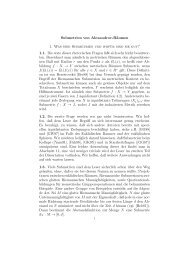
Figure 1: The contact structure ker(dz + x dy).<br />
Definition 2.8. Two contact manifolds (M1, ξ1) and (M2, ξ2) are called contac-<br />
tomorphic if there is a diffeomorphism f : M1 → M2 with Tf(ξ1) = ξ2, where<br />
Tf : TM1 → TM2 denotes the differential of f. If ξi = kerαi, i = 1, 2, this<br />
is equivalent to the existence of a nowhere zero function λ: M1 → R such that<br />
f ∗ α2 = λα1.<br />
Example 2.9. The contact manifolds (R 2n+1 , ξi = kerαi), i = 1, 2, from the<br />
preceding examples are contactomorphic. An explicit contactomorphism f with<br />
f ∗ α2 = α1 is given by<br />
f(x, y, z) = � (x + y)/2, (y − x)/2, z + xy/2 � ,<br />
where x and y stand for (x1, . . .,xn) and (y1, . . .,yn), respectively, and xy stands<br />
for �<br />
j xjyj. Similarly, both these contact structures are contactomorphic to<br />
ker(dz − �<br />
j yj dxj). Any of these contact structures is called the standard<br />
contact structure on R 2n+1 .<br />
Example 2.10. The standard contact structure on the unit sphere S 2n+1<br />
in R 2n+2 (with cartesian coordinates (x1, y1, . . .,xn+1, yn+1)) is defined by the<br />
contact form<br />
n+1 �<br />
α0 = (xj dyj − yj dxj).<br />
j=1<br />
With r denoting the radial coordinate on R2n+2 (that is, r2 = �<br />
j (x2j + y2 j )) one<br />
checks easily that α0 ∧ (dα0) n ∧ r dr �= 0 for r �= 0. Since S2n+1 is a level surface<br />
of r (or r 2 ), this verifies the contact condition.<br />
7<br />
y
Alternatively, one may regard S 2n+1 as the unit sphere in C n+1 with complex<br />
structure J (corresponding to complex coordinates zj = xj+iyj, j = 1, . . .,n+1).<br />
Then ξ0 = kerα0 defines at each point p ∈ S 2n+1 the complex (i.e. J–invariant)<br />
subspace of TpS 2n+1 , that is,<br />
ξ0 = TS 2n+1 ∩ J(TS 2n+1 ).<br />
This follows from the observation that α = −r dr◦J. The hermitian form dα(., J.)<br />
on ξ0 is called the Levi form of the hypersurface S 2n+1 ⊂ C n+1 . The contact<br />
condition for ξ corresponds to the positive definiteness of that Levi form, or what<br />
in complex analysis is called the strict pseudoconvexity of the hypersurface. For<br />
more on the question of pseudoconvexity from the contact geometric viewpoint<br />
see [1, Section 8.2]. Beware that the ‘complex structure’ in their Proposition 8.14<br />
is not required to be integrable, i.e. constitutes what is more commonly referred<br />
to as an ‘almost complex structure’.<br />
Definition 2.11. Let (V, ω) be a symplectic manifold of dimension 2n + 2,<br />
that is, ω is a closed (dω = 0) and non-degenerate (ω n+1 �= 0) 2–form on V . A<br />
vector field X is called a Liouville vector field if LXω = ω, where L denotes<br />
the Lie <strong>der</strong>ivative.<br />
With the help of Cartan’s formula LX = d ◦ iX + iX ◦ d this may be rewrit-<br />
ten as d(iXω) = ω. Then the 1–form α = iXω defines a contact form on any<br />
hypersurface M in V transverse to X. Indeed,<br />
α ∧ (dα) n = iXω ∧ (d(iXω)) n = iXω ∧ ω n = 1<br />
n + 1 iX(ω n+1 ),<br />
which is a volume form on M ⊂ V provided M is transverse to X.<br />
Example 2.12. With V = R 2n+2 , symplectic form ω = �<br />
j dxj ∧ dyj, and<br />
Liouville vector field X = �<br />
j (xj∂xj + yj∂yj )/2 = r∂r/2, we recover the standard<br />
contact structure on S 2n+1 .<br />
For finer issues relating to hypersurfaces in symplectic manifolds transverse<br />
to a Liouville vector field I refer the rea<strong>der</strong> to [1, Section 8.2].<br />
Here is a further useful example of contactomorphic manifolds.<br />
Proposition 2.13. For any point p ∈ S 2n+1 , the manifold (S 2n+1 \ {p}, ξ0) is<br />
contactomorphic to (R 2n+1 , ξ2).<br />
8
Proof. The contact manifold (S 2n+1 , ξ0) is a homogeneous space un<strong>der</strong> the nat-<br />
ural U(n + 1)–action, so we are free to choose p = (0, . . .,0, −1). Stereographic<br />
projection from p does almost, but not quite yield the desired contactomorphism.<br />
Instead, we use a map that is well-known in the theory of Siegel domains (cf. [3,<br />
Chapter 8]) and that looks a bit like a complex analogue of stereographic projec-<br />
tion; this was suggested in [92, Exercise 3.64].<br />
Regard S 2n+1 as the unit sphere in C n+1 = C n ×C with cartesian coordinates<br />
(z1, . . .,zn, w) = (z, w). We identify R 2n+1 with C n ×R ⊂ C n ×C with coordinates<br />
(ζ1, . . .,ζn, s) = (ζ, s) = (ζ,Re σ), where ζj = xj + iyj. Then<br />
n�<br />
α2 = ds + (xj dyj − yj dxj)<br />
and<br />
j=1<br />
= ds + i<br />
(ζ dζ − ζ dζ).<br />
2<br />
α0 = i<br />
(z dz − z dz + w dw − w dw).<br />
2<br />
Now define a smooth map f : S 2n+1 \ {(0, −1)} → R 2n+1 by<br />
Then<br />
and<br />
(ζ, s) = f(z, w) =<br />
�<br />
z i(w − w)<br />
, −<br />
1 + w 2|1 + w| 2<br />
�<br />
.<br />
f ∗ i dw i dw<br />
ds = − +<br />
2|1 + w| 2 2|1 + w| 2<br />
+ i(w − w) dw i(w − w) dw<br />
+<br />
2(1 + w) |1 + w| 2 2(1 + w) |1 + w| 2<br />
i<br />
=<br />
2|1 + w| 2<br />
�<br />
w − w w − w<br />
−dw + dw + dw +<br />
1 + w 1 + w dw<br />
�<br />
f ∗ (ζ dζ − ζ dζ) =<br />
Along S 2n+1 we have<br />
=<br />
�<br />
z dz<br />
1 + w<br />
− z<br />
�<br />
dz<br />
z<br />
(1 + w) 2dw<br />
�<br />
1 + w −<br />
1 + w 1 + w −<br />
z<br />
(1 + w) 2dw<br />
�<br />
1<br />
|1 + w| 2<br />
�<br />
z dz − zdz + |z| 2<br />
� ��<br />
dw dw<br />
− .<br />
1 + w 1 + w<br />
|z| 2 = 1 − |w| 2 = (1 − w)(1 + w) + (w − w)<br />
= (1 − w)(1 + w) − (w − w),<br />
9
whence<br />
|z| 2<br />
� �<br />
dw dw<br />
−<br />
1 + w 1 + w<br />
w − w<br />
= (1 − w)dw −<br />
1 + w dw<br />
w − w<br />
− (1 − w)dw −<br />
1 + w dw.<br />
From these calculations we conclude f ∗ α2 = α0/|1 + w| 2 . So it only remains to<br />
show that f is actually a diffeomorphism of S 2n+1 \ {(0, −1)} onto R 2n+1 . To<br />
that end, consi<strong>der</strong> the map<br />
defined by<br />
�f : (C n × C) \ (C n × {−1}) −→ (C n × C) \ (C n × {−i/2})<br />
(ζ, σ) = � f(z, w) =<br />
� �<br />
z i w − 1<br />
, − .<br />
1 + w 2 w + 1<br />
This is a biholomorphic map with inverse map<br />
� �<br />
2ζ 1 + 2iσ<br />
(ζ, σ) ↦−→ , .<br />
1 − 2iσ 1 − 2iσ<br />
We compute<br />
w − 1 w − 1<br />
Im σ = − −<br />
4(w + 1) 4(w + 1)<br />
(w − 1)(w + 1) + (w − 1)(w + 1)<br />
= −<br />
4|1 + w| 2<br />
= 1 − |w|2<br />
2|1 + w| 2.<br />
Hence for (z, w) ∈ S 2n+1 \ {(0, −1)} we have<br />
Imσ =<br />
|z| 2 1<br />
=<br />
2|1 + w| 2 2 |ζ|2 ;<br />
conversely, any point (ζ, σ) with Imσ = |ζ| 2 /2 lies in the image of � f| S 2n+1 \{(0,−1)},<br />
that is, � f restricted to S 2n+1 \{(0, −1)} is a diffeomorphism onto {Im σ = |ζ| 2 /2}.<br />
Finally, we compute<br />
i(w − 1) i(w − 1)<br />
Re σ = − +<br />
4(w + 1) 4(w + 1)<br />
(w − 1)(w + 1) − (w − 1)(w + 1)<br />
= −i<br />
4|1 + w| 2<br />
i(w − w)<br />
= −<br />
2|1 + w| 2,<br />
10
from which we see that for (z, w) ∈ S 2n+1 \ {(0, −1)} and with (ζ, σ) = � f(z, w)<br />
we have f(z, w) = (ζ,Re σ). This concludes the proof.<br />
At the beginning of this section I mentioned that one may allow contact<br />
structures that are not coorientable, and hence not defined by a global contact<br />
form.<br />
Example 2.14. Let M = R n+1 ×RP n with cartesian coordinates (x0, . . .,xn) on<br />
the R n+1 –factor and homogeneous coordinates [y0 : . . . : yn] on the RP n –factor.<br />
Then<br />
ξ = ker � n �<br />
j=0<br />
�<br />
yj dxj<br />
is a well-defined hyperplane field on M, because the 1–form on the right-hand side<br />
is well-defined up to scaling by a non-zero real constant. On the open submanifold<br />
Uk = {yk �= 0} ∼ = Rn+1 × Rn of M we have ξ = kerαk with<br />
αk = dxk + �<br />
� �<br />
yj<br />
dxj<br />
j�=k<br />
an honest 1–form on Uk. This is the standard contact form of Example 2.6, which<br />
proves that ξ is a contact structure on M.<br />
If n is even, then M is not orientable, so there can be no global contact<br />
form defining ξ (cf. Remark 2.2), i.e. ξ is not coorientable. Notice, however, that<br />
a contact structure on a manifold of dimension 2n + 1 with n even is always<br />
orientable: the sign of (dα) n |ξ does not depend on the choice of local 1–form<br />
defining ξ.<br />
If n is odd, then M is orientable, so it would be possible that ξ is the kernel<br />
of a globally defined 1–form. However, since the sign of α ∧ (dα) n , for n odd, is<br />
independent of the choice of local 1–form defining ξ, it is also conceivable that no<br />
global contact form exists. (In fact, this consi<strong>der</strong>ation shows that any manifold<br />
of dimension 2n + 1, with n odd, admitting a contact structure (coorientable or<br />
not) needs to be orientable.) This is indeed what happens, as we shall prove now.<br />
Proposition 2.15. Let (M, ξ) be the contact manifold of the preceding example.<br />
Then TM/ξ can be identified with the canonical line bundle on RP n (pulled back<br />
to M). In particular, TM/ξ is a non-trivial line bundle, so ξ is not coorientable.<br />
11<br />
yk
Proof. For given y = [y0 : . . . : yn] ∈ RP n , the vector y0∂x0 +· · ·+yn∂xn ∈ TxR n+1<br />
is well-defined up to a non-zero real factor (and independent of x ∈ R n+1 ), and<br />
hence defines a line ℓy in TxR n+1 ∼ = R n+1 . The set<br />
E = {(t, x, y): x ∈ R n+1 , y ∈ RP n , t ∈ ℓy}<br />
⊂ TR n+1 × RP n ⊂ T(R n+1 × RP n ) = TM<br />
with projection (t, x, y) ↦→ (x, y) defines a line sub-bundle of TM that restricts<br />
to the canonical line bundle over {x} × RP n ≡ RP n for each x ∈ R n+1 . The<br />
canonical line bundle over RP n is well-known to be non-trivial [95, p. 16], so the<br />
same holds for E.<br />
Moreover, E is clearly complementary to ξ, i.e. TM/ξ ∼ = E, since<br />
n�<br />
j=0<br />
yj dxj(<br />
n�<br />
k=0<br />
yk∂xk ) =<br />
This proves that that ξ is not coorientable.<br />
n�<br />
j=0<br />
y 2 j �= 0.<br />
To sum up, in the example above we have one of the following two situations:<br />
• If n is odd, then M is orientable; ξ is neither orientable nor coorientable.<br />
• If n is even, then M is not orientable; ξ is not coorientable, but it is ori-<br />
entable.<br />
We close this section with the definition of the most important types of sub-<br />
manifolds.<br />
Definition 2.16. Let (M, ξ) be a contact manifold.<br />
(i) A submanifold L of (M, ξ) is called an isotropic submanifold if TxL ⊂ ξx<br />
for all x ∈ L.<br />
(ii) A submanifold M ′ of M with contact structure ξ ′ is called a contact<br />
submanifold if TM ′ ∩ ξ|M ′ = ξ′ .<br />
Observe that if ξ = kerα and i: M ′ → M denotes the inclusion map, then the<br />
condition for (M ′ , ξ ′ ) to be a contact submanifold of (M, ξ) is that ξ ′ = ker(i ∗ α).<br />
In particular, ξ ′ ⊂ ξ|M ′ is a symplectic sub-bundle with respect to the symplectic<br />
bundle structure on ξ given by dα.<br />
The following is a manifestation of the maximal non-integrability of contact<br />
structures.<br />
12
Proposition 2.17. Let (M, ξ) be a contact manifold of dimension 2n + 1 and L<br />
an isotropic submanifold. Then dim L ≤ n.<br />
Proof. Write i for the inclusion of L in M and let α be an (at least locally<br />
defined) contact form defining ξ. Then the condition for L to be isotropic becomes<br />
i ∗ α ≡ 0. It follows that i ∗ dα ≡ 0. In particular, TpL ⊂ ξp is an isotropic<br />
subspace of the symplectic vector space (ξp, dα|ξp ), i.e. a subspace on which the<br />
symplectic form restricts to zero. From Linear Algebra we know that this implies<br />
dimTpL ≤ (dimξp)/2 = n.<br />
Definition 2.18. An isotropic submanifold L ⊂ (M 2n+1 , ξ) of maximal possible<br />
dimension n is called a Legendrian submanifold.<br />
In particular, in a 3–dimensional contact manifold there are two distinguished<br />
types of knots: Legendrian knots on the one hand, transverse 1 knots on the<br />
other, i.e. knots that are everywhere transverse to the contact structure. If ξ<br />
is cooriented by a contact form α and γ : S 1 → (M, ξ = kerα) is oriented, one<br />
can speak of a positively or negatively transverse knot, depending on whether<br />
α(˙γ) > 0 or α(˙γ) < 0.<br />
2.2 Gray stability and the Moser trick<br />
The Gray stability theorem that we are going to prove in this section says that<br />
there are no non-trivial deformations of contact structures on closed manifolds.<br />
In fancy language, this means that contact structures on closed manifolds have<br />
discrete moduli. First a preparatory lemma.<br />
Lemma 2.19. Let ωt, t ∈ [0, 1], be a smooth family of differential k–forms on a<br />
manifold M and (ψt) t∈[0,1] an isotopy of M. Define a time-dependent vector field<br />
Xt on M by Xt ◦ ψt = ˙ ψt, where the dot denotes <strong>der</strong>ivative with respect to t (so<br />
that ψt is the flow of Xt). Then<br />
d � � � � ∗ ∗<br />
ψt ωt = ψt ˙ωt + LXtωt .<br />
dt<br />
Proof. For a time-independent k–form ω we have<br />
d � ∗<br />
ψt ω<br />
dt<br />
� = ψ ∗� t LXtω � .<br />
This follows by observing that<br />
1 Some people like to call them ‘transversal knots’, but I adhere to J.H.C. Whitehead’s dictum,<br />
as quoted in [64]: “Transversal is a noun; the adjective is transverse.”<br />
13
(i) the formula holds for functions,<br />
(ii) if it holds for differential forms ω and ω ′ , then also for ω ∧ ω ′ ,<br />
(iii) if it holds for ω, then also for dω,<br />
(iv) locally functions and differentials of functions generate the algebra of dif-<br />
ferential forms.<br />
We then compute<br />
d<br />
dt (ψ∗ ψ<br />
t ωt) = lim<br />
h→0<br />
∗ t+hωt+h − ψ∗ t ωt<br />
h<br />
= lim<br />
h→0<br />
ψ ∗ t+h ωt+h − ψ ∗ t+h ωt + ψ ∗ t+h ωt − ψ ∗ t ωt<br />
= lim ψ<br />
h→0 ∗ � �<br />
ωt+h − ωt<br />
t+h + lim<br />
h h→0<br />
� �<br />
˙ωt + LXtωt .<br />
= ψ ∗ t<br />
h<br />
ψ ∗ t+h ωt − ψ ∗ t ωt<br />
h<br />
For that last equality observe (regarding the second summand) that ψt+h =<br />
ψt h ◦ ψt, where ψt h<br />
dependent vector field Xt h := Xt+h; then apply the result for time-independent<br />
k–forms.<br />
denotes, for fixed t and time-variable h, the flow of the time-<br />
Theorem 2.20 (Gray stability). Let ξt, t ∈ [0, 1], be a smooth family of contact<br />
structures on a closed manifold M. Then there is an isotopy (ψt) t∈[0,1] of M such<br />
that<br />
Tψt(ξ0) = ξt for each t ∈ [0, 1].<br />
Proof. The simplest proof of this result rests on what is known as the Moser<br />
trick, introduced by J. Moser [96] in the context of stability results for (equicoho-<br />
mologous) volume and symplectic forms. J. Gray’s original proof [61] was based<br />
on deformation theory à la Kodaira-Spencer. The idea of the Moser trick is to<br />
assume that ψt is the flow of a time-dependent vector field Xt. The desired equa-<br />
tion for ψt then translates into an equation for Xt. If that equation can be solved,<br />
the isotopy ψt is found by integrating Xt; on a closed manifold the flow of Xt will<br />
be globally defined.<br />
Let αt be a smooth family of 1–forms with kerαt = ξt. The equation in the<br />
theorem then translates into<br />
ψ ∗ t αt = λtα0,<br />
14
where λt: M → R + is a suitable smooth family of smooth functions. Differen-<br />
tiation of this equation with respect to t yields, with the help of the preceding<br />
lemma,<br />
ψ ∗� �<br />
t ˙αt + LXtαt = λtα0<br />
˙ = ˙ λt<br />
ψ<br />
λt<br />
∗ t αt,<br />
or, with the help of Cartan’s formula LX = d ◦ iX + iX ◦ d and with µt =<br />
d<br />
dt (log λt) ◦ ψ −1<br />
t ,<br />
ψ ∗� � ∗<br />
t ˙αt + d(αt(Xt)) + iXtdαt = ψt (µtαt).<br />
If we choose Xt ∈ ξt, this equation will be satisfied if<br />
Plugging in the Reeb vector field Rαt gives<br />
˙αt + iXtdαt = µtαt. (2.1)<br />
˙αt(Rαt) = µt. (2.2)<br />
So we can use (2.2) to define µt, and then the non-degeneracy of dαt|ξt and<br />
the fact that Rαt ∈ ker(µtαt − ˙αt) allow us to find a unique solution Xt ∈ ξt<br />
of (2.1).<br />
Remark 2.21. (1) <strong>Contact</strong> forms do not satisfy stability, that is, in general<br />
one cannot find an isotopy ψt such that ψ ∗ t αt = α0. For instance, consi<strong>der</strong> the<br />
following family of contact forms on S 3 ⊂ R 4 :<br />
αt = (x1 dy1 − y1 dx1) + (1 + t)(x2 dy2 − y2 dx2),<br />
where t ≥ 0 is a real parameter. The Reeb vector field of αt is<br />
Rαt = (x1 ∂y1 − y1<br />
1<br />
∂x1 ) +<br />
1 + t (x2 ∂y2 − y2 ∂x2 ).<br />
The flow of Rα0 defines the Hopf fibration, in particular all orbits of Rα0 are<br />
closed. For t ∈ R + \ Q, on the other hand, Rαt has only two periodic orbits. So<br />
there can be no isotopy with ψ ∗ t αt = α0, because such a ψt would also map Rα0<br />
to Rαt.<br />
(2) Y. Eliashberg [25] has shown that on the open manifold R 3 there are<br />
likewise no non-trivial deformations of contact structures, but on S 1 × R 2 there<br />
does exist a continuum of non-equivalent contact structures.<br />
(3) For further applications of this theorem it is useful to observe that at<br />
points p ∈ M with ˙αt,p identically zero in t we have Xt(p) ≡ 0, so such points<br />
remain stationary un<strong>der</strong> the isotopy ψt.<br />
15
2.3 <strong>Contact</strong> Hamiltonians<br />
A vector field X on the contact manifold (M, ξ = kerα) is called an infinitesi-<br />
mal automorphism of the contact structure if the local flow of X preserves ξ<br />
(The study of such automorphisms was initiated by P. Libermann, cf. [80]). By<br />
slight abuse of notation, we denote this flow by ψt; if M is not closed, ψt (for a<br />
fixed t �= 0) will not in general be defined on all of M. The condition for X to<br />
be an infinitesimal automorphism can be written as Tψt(ξ) = ξ, which is equiv-<br />
alent to LXα = λα for some function λ: M → R (notice that this condition is<br />
independent of the choice of 1–form α defining ξ). The local flow of X preserves<br />
α if and only if LXα = 0.<br />
Theorem 2.22. With a fixed choice of contact form α there is a one-to-one<br />
correspondence between infinitesimal automorphisms X of ξ = kerα and smooth<br />
functions H : M → R. The correspondence is given by<br />
• X ↦−→ HX = α(X);<br />
• H ↦−→ XH, defined uniqely by α(XH) = H and iXH dα = dH(Rα)α − dH.<br />
The fact that XH is uniquely defined by the equations in the theorem follows<br />
as in the preceding section from the fact that dα is non-degenerate on ξ and<br />
Rα ∈ ker(dH(Rα)α − dH).<br />
Proof. Let X be an infinitesimal automorphism of ξ. Set HX = α(X) and write<br />
dHX + iXdα = LXα = λα with λ: M → R. Applying this last equation to<br />
Rα yields dHX(Rα) = λ. So X satisfies the equations α(X) = HX and iXdα =<br />
dHX(Rα)α − dHX. This means that XHX = X.<br />
Conversely, given H : M → R and with XH as defined in the theorem, we<br />
have<br />
LXH α = iXH dα + d(α(XH)) = dH(Rα)α,<br />
so XH is an infinitesimal automorphism of ξ. Moreover, it is immediate from the<br />
definitions that HXH = α(XH) = H.<br />
Corollary 2.23. Let (M, ξ = kerα) be a closed contact manifold and Ht: M →<br />
R, t ∈ [0, 1], a smooth family of functions. Let Xt = XHt be the correspond-<br />
ing family of infinitesimal automorphisms of ξ (defined via the correspondence<br />
described in the preceding theorem). Then the globally defined flow ψt of the<br />
16
time-dependent vector field Xt is a contact isotopy of (M, ξ), that is, ψ ∗ t α = λtα<br />
for some smooth family of functions λt: M → R + .<br />
Proof. With Lemma 2.19 and the preceding proof we have<br />
d � ∗<br />
ψt α<br />
dt<br />
� = ψ ∗� t LXtα � = ψ ∗� t dHt(Rα)α � = µtψ ∗ t α<br />
with µt = dHt(Rα) ◦ ψt. Since ψ0 = idM (whence ψ∗ 0α = α) this implies that,<br />
with<br />
we have ψ ∗ t α = λtα.<br />
λt = exp �� t<br />
µs ds � ,<br />
0<br />
This corollary will be used in Section 2.5 to prove various isotopy extension<br />
theorems from isotopies of special submanifolds to isotopies of the ambient con-<br />
tact manifold. In a similar vein, contact Hamiltonians can be used to show that<br />
standard general position arguments from differential topology continue to hold<br />
in the contact geometric setting. Another application of contact Hamiltonians<br />
is a proof of the fact that the contactomorphism group of a connected contact<br />
manifold acts transitively on that manifold [12]. (See [8] for more on the general<br />
structure of contactomorphism groups.)<br />
2.4 Darboux’s theorem and neighbourhood theorems<br />
The flexibility of contact structures inherent in the Gray stability theorem and<br />
the possibility to construct contact isotopies via contact Hamiltonians results in<br />
a variety of theorems that can be summed up as saying that there are no local<br />
invariants in contact geometry. Such theorems form the theme of the present<br />
section.<br />
In contrast with Riemannian geometry, for instance, where the local structure<br />
coming from the curvature gives rise to a rich theory, the interesting questions<br />
in contact geometry thus appear only at the global level. However, it is actually<br />
that local flexibility that allows us to prove strong global theorems, such as the<br />
existence of contact structures on certain closed manifolds.<br />
2.4.1 Darboux’s theorem<br />
Theorem 2.24 (Darboux’s theorem). Let α be a contact form on the (2n +<br />
1)–dimensional manifold M and p a point on M. Then there are coordinates<br />
17
x1, . . .,xn, y1, . . .,yn, z on a neighbourhood U ⊂ M of p such that<br />
α|U = dz +<br />
n�<br />
j=1<br />
xj dyj.<br />
Proof. We may assume without loss of generality that M = R 2n+1 and p = 0 is<br />
the origin of R 2n+1 . Choose linear coordinates x1, . . .,xn, y1, . . .yn, z on R 2n+1<br />
such that<br />
on T0R 2n+1 :<br />
�<br />
α(∂z) = 1, i∂zdα = 0,<br />
∂xj , ∂yj ∈ kerα (j = 1, . . .,n), dα = � n<br />
j=1 dxj ∧ dyj.<br />
This is simply a matter of linear algebra (the normal form theorem for skew-<br />
symmetric forms on a vector space).<br />
Now set α0 = dz + �<br />
j xj dyj and consi<strong>der</strong> the family of 1–forms<br />
αt = (1 − t)α0 + tα, t ∈ [0, 1],<br />
on R 2n+1 . Our choice of coordinates ensures that<br />
αt = α, dαt = dα at the origin.<br />
Hence, on a sufficiently small neighbourhood of the origin, αt is a contact form<br />
for all t ∈ [0, 1].<br />
We now want to use the Moser trick to find an isotopy ψt of a neighbourhood<br />
of the origin such that ψ ∗ t αt = α0. This aim seems to be in conflict with our<br />
earlier remark that contact forms are not stable, but as we shall see presently,<br />
locally this equation can always be solved.<br />
Indeed, differentiating ψ ∗ t αt = α0 (and assuming that ψt is the flow of some<br />
time-dependent vector field Xt) we find<br />
so Xt needs to satisfy<br />
ψ ∗� �<br />
t ˙αt + LXtαt = 0,<br />
˙αt + d(αt(Xt)) + iXtdαt = 0. (2.3)<br />
Write Xt = HtRαt + Yt with Yt ∈ ker αt. Inserting Rαt in (2.3) gives<br />
˙αt(Rαt) + dHt(Rαt) = 0. (2.4)<br />
18
On a neighbourhood of the origin, a smooth family of functions Ht satisfying<br />
(2.4) can always be found by integration, provided only that this neighbourhood<br />
has been chosen so small that none of the Rαt has any closed orbits there. Since<br />
αt ˙ is zero at the origin, we may require that Ht(0) = 0 and dHt|0 = 0 for all<br />
t ∈ [0, 1]. Once Ht has been chosen, Yt is defined uniquely by (2.3), i.e. by<br />
˙αt + dHt + iYtdαt = 0.<br />
Notice that with our assumptions on Ht we have Xt(0) = 0 for all t.<br />
Now define ψt to be the local flow of Xt. This local flow fixes the origin, so<br />
there it is defined for all t ∈ [0, 1]. Since the domain of definition in R × M of a<br />
local flow on a manifold M is always open (cf. [15, 8.11]), we can infer 2 that ψt<br />
is actually defined for all t ∈ [0, 1] on a sufficiently small neighbourhood of the<br />
origin in R 2n+1 . This concludes the proof of the theorem (strictly speaking, the<br />
local coordinates in the statement of the theorem are the coordinates xj ◦ ψ −1<br />
1<br />
etc.).<br />
Remark 2.25. The proof of this result given in [1] is incomplete: It is not<br />
possible, as is suggested there, to prove the Darboux theorem for contact forms<br />
if one requires Xt ∈ ker αt.<br />
2.4.2 Isotropic submanifolds<br />
Let L ⊂ (M, ξ = kerα) be an isotropic submanifold in a contact manifold with<br />
cooriented contact structure. Write (TL) ⊥ ⊂ ξ|L for the sub-bundle of ξ|L that is<br />
symplectically orthogonal to TL with respect to the symplectic bundle structure<br />
dα|ξ. The conformal class of this symplectic bundle structure depends only on<br />
the contact structure ξ, not on the choice of contact form α defining ξ: If α is<br />
replaced by λα for some smooth function λ: M → R + , then d(λα)|ξ = λ dα|ξ.<br />
So the bundle (TL) ⊥ is determined by ξ.<br />
The fact that L is isotropic implies TL ⊂ (TL) ⊥ . Following Weinstein [105],<br />
we call the quotient bundle (TL) ⊥ /TL with the conformal symplectic structure<br />
induced by dα the conformal symplectic normal bundle of L in M and write<br />
CSN(M, L) = (TL) ⊥ /TL.<br />
2 To be absolutely precise, one ought to work with a family αt, t ∈ R, where αt ≡ α0 for<br />
t ≤ ε and αt ≡ α1 for t ≥ 1 − ε, i.e. a technical homotopy in the sense of [15]. Then Xt will be<br />
defined for all t ∈ R, and the reasoning of [15] can be applied.<br />
19
So the normal bundle NL = (TM|L)/TL of L in M can be split as<br />
NL ∼ = (TM|L)/(ξ|L) ⊕ (ξ|L)/(TL) ⊥ ⊕ CSN(M, L).<br />
Observe that if dimM = 2n + 1 and dimL = k ≤ n, then the ranks of the<br />
three summands in this splitting are 1, k and 2(n − k), respectively. Our aim<br />
in this section is to show that a neighbourhood of L in M is determined, up to<br />
contactomorphism, by the isomorphism type (as a conformal symplectic bundle)<br />
of CSN(M, L).<br />
The bundle (TM|L)/(ξ|L) is a trivial line bundle because ξ is cooriented.<br />
The bundle (ξ|L)/(TL) ⊥ can be identified with the cotangent bundle T ∗ L via the<br />
well-defined bundle isomorphism<br />
Ψ: (ξ|L)/(TL) ⊥ −→ T ∗ L<br />
Y ↦−→ iY dα|TL.<br />
(Ψ is obviously injective and well-defined by the definition of (TL) ⊥ , and the<br />
ranks of the two bundles are equal.)<br />
Although Ψ is well-defined on the quotient (ξ|L)/(TL) ⊥ , to proceed further<br />
we need to choose an isotropic complement of (TL) ⊥ in ξ|L. Restricted to each<br />
fibre ξp, p ∈ L, such an isotropic complement of (TpL) ⊥ exists. There are two<br />
ways to obtain a smooth bundle of such isotropic complements. The first would<br />
be to carry over Arnold’s corresponding discussion of Lagrangian subbundles<br />
of symplectic bundles [6] to the isotropic case in or<strong>der</strong> to show that the space<br />
of isotropic complements of U ⊥ ⊂ V , where U is an isotropic subspace in a<br />
symplectic vector space V , is convex. (This argument uses generating functions<br />
for isotropic subspaces.) Then by a partition of unity argument the desired<br />
complement can be constructed on the bundle level.<br />
A slightly more pedestrian approach is to define this isotropic complement<br />
with the help of a complex bundle structure J on ξ compatible with dα (cf.<br />
Remark 2.3). The condition dα(X, JX) > 0 for 0 �= X ∈ ξ implies that (TpL) ⊥ ∩<br />
J(TpL) = {0} for all p ∈ L, and so a dimension count shows that J(TL) is indeed<br />
a complement of (TL) ⊥ in ξ|L. (In a similar vein, CSN(M, L) can be identified<br />
as a sub-bundle of ξ, viz., the orthogonal complement of TL ⊕ J(TL) ⊂ ξ with<br />
respect to the bundle metric dα(., J.) on ξ.)<br />
On the Whitney sum TL ⊕ T ∗ L (for any manifold L) there is a canonical<br />
symplectic bundle structure ΩL defined by<br />
ΩL,p(X + η, X ′ + η ′ ) = η(X ′ ) − η ′ (X) for X, X ′ ∈ TpL; η, η ′ ∈ T ∗ p L.<br />
20
Lemma 2.26. The bundle map<br />
idTL ⊕ Ψ: (TL ⊕ J(TL), dα) −→ (TL ⊕ T ∗ L,ΩL)<br />
is an isomorphism of symplectic vector bundles.<br />
Proof. We only need to check that idTL ⊕ Ψ is a symplectic bundle map. Let<br />
X, X ′ ∈ TpL and Y, Y ′ ∈ Jp(TpL). Write Y = JpZ, Y ′ = JpZ ′ with Z, Z ′ ∈ TpL.<br />
It follows that<br />
dα(Y, Y ′ ) = dα(JZ, JZ ′ ) = dα(Z, Z ′ ) = 0,<br />
since L is an isotropic submanifold. For the same reason dα(X, X ′ ) = 0. Hence<br />
dα(X + Y, X ′ + Y ′ ) = dα(Y, X ′ ) − dα(Y ′ , X)<br />
= Ψ(Y )(X ′ ) − Ψ(Y ′ )(X)<br />
= ΩL(X + Ψ(Y ), X ′ + Ψ(Y ′ )).<br />
Theorem 2.27. Let (Mi, ξi), i = 0, 1, be contact manifolds with closed isotropic<br />
submanifolds Li. Suppose there is an isomorphism of conformal symplectic nor-<br />
mal bundles Φ: CSN(M0, L0) → CSN(M1, L1) that covers a diffeomorphism<br />
φ: L0 → L1. Then φ extends to a contactomorphism ψ: N(L0) → N(L1) of<br />
suitable neighbourhoods N(Li) of Li such that Tψ| CSN(M0,L0) and Φ are bundle<br />
homotopic (as symplectic bundle isomorphisms).<br />
Corollary 2.28. Diffeomorphic (closed) Legendrian submanifolds have contac-<br />
tomorphic neighbourhoods.<br />
Proof. If Li ⊂ Mi is Legendrian, then CSN(Mi, Li) has rank 0, so the conditions<br />
in the theorem, apart from the existence of a diffeomorphism φ: L0 → L1, are<br />
void.<br />
Example 2.29. Let S 1 ⊂ (M 3 , ξ) be a Legendrian knot in a contact 3–manifold.<br />
Then with a coordinate θ ∈ [0, 2π] along S 1 and coordinates x, y in slices trans-<br />
verse to S 1 , the contact structure<br />
cos θ dx − sin θ dy = 0<br />
provides a model for a neighbourhood of S 1 .<br />
21
Proof of Theorem 2.27. Choose contact forms αi for ξi, i = 0, 1, scaled in such a<br />
way that Φ is actually an isomorphism of symplectic vector bundles with respect<br />
to the symplectic bundle structures on CSN(Mi, Li) given by dαi. Here we think<br />
of CSN(Mi, Li) as a sub-bundle of TMi|Li (rather than as a quotient bundle).<br />
We identify (TMi|Li )/(ξi|Li ) with the trivial line bundle spanned by the Reeb<br />
vector field Rαi . In total, this identifies<br />
as a sub-bundle of TMi|Li .<br />
NLi = 〈Rαi 〉 ⊕ Ji(TLi) ⊕ CSN(Mi, Li)<br />
Let ΦR: 〈Rα0 〉 → 〈Rα1 〉 be the obvious bundle isomorphism defined by requiring<br />
that Rα0 (p) map to Rα1 (φ(p)).<br />
Let Ψi: Ji(TLi) → T ∗Li be the isomorphism defined by taking the interior<br />
product with dαi. Notice that<br />
Tφ ⊕ (φ ∗ ) −1 : (TL0 ⊕ T ∗ L0, ΩL0 ) → (TL1 ⊕ T ∗ L1, ΩL1 )<br />
is an isomorphism of symplectic vector bundles. With Lemma 2.26 it follows that<br />
Tφ ⊕ Ψ −1<br />
1 ◦ (φ∗ ) −1 ◦ Ψ0: (TL0 ⊕ J0(TL0), dα0) → (TL1 ⊕ J1(TL1), dα1)<br />
is an isomorphism of symplectic vector bundles.<br />
Now let<br />
�Φ: NL0 −→ NL1<br />
be the bundle isomorphism (covering φ) defined by<br />
�Φ = ΦR ⊕ Ψ −1<br />
1 ◦ (φ∗ ) −1 ◦ Ψ0 ⊕ Φ.<br />
Let τi: NLi → Mi be tubular maps, that is, the τ (I suppress the index i for<br />
better readability) are embeddings such that τ|L – where L is identified with the<br />
zero section of NL – is the inclusion L ⊂ M, and Tτ induces the identity on NL<br />
along L (with respect to the splittings T(NL)|L = TL ⊕ NL = TM|L).<br />
Then τ1 ◦ � Φ ◦ τ −1<br />
0 : N(L0) → N(L1) is a diffeomorphism of suitable neighbourhoods<br />
N(Li) of Li that induces the bundle map<br />
Tφ ⊕ � Φ: TM0|L0 −→ TM1|L1 .<br />
By construction, this bundle map pulls α1 back to α0 and dα1 to dα0. Hence, α0<br />
and (τ1 ◦ � Φ ◦ τ −1<br />
0 )∗α1 are contact forms on N(L0) that coincide on TM0|L0 , and<br />
so do their differentials.<br />
22
Now consi<strong>der</strong> the family of 1–forms<br />
βt = (1 − t)α0 + t(τ1 ◦ � Φ ◦ τ −1<br />
0 )∗ α1, t ∈ [0, 1].<br />
On TM0|L0 we have βt ≡ α0 and dβt ≡ dα0. Since the contact condition α ∧<br />
(dα) n �= 0 is an open condition, we may assume – shrinking N(L0) if necessary<br />
– that βt is a contact form on N(L0) for all t ∈ [0, 1]. By the Gray stability<br />
theorem (Thm. 2.20) and Remark 2.21 (3) following its proof, we find an isotopy<br />
ψt of N(L0), fixing L0, such that ψ ∗ t βt = λtα0 for some smooth family of smooth<br />
functions λt: N(L0) → R + .<br />
(Since N(L0) is not a closed manifold, ψt is a priori only a local flow. But<br />
on L0 it is stationary and hence defined for all t. As in the proof of the Darboux<br />
theorem (Thm. 2.24) we conclude that ψt is defined for all t ∈ [0, 1] in a sufficiently<br />
small neighbourhood of L0, so shrinking N(L0) once again, if necessary, will<br />
ensure that ψt is a global flow on N(L0).)<br />
We conclude that ψ = τ1 ◦ � Φ ◦ τ −1<br />
0 ◦ ψ1 is the desired contactomorphism.<br />
Remark 2.30. With a little more care one can actually achieve Tψ1 = id on<br />
TM0|L0 , which implies in particular that Tψ| CSN(M0,L0) = Φ, cf. [105]. (Remem-<br />
ber that there is a certain freedom in constructing an isotopy via the Moser trick<br />
if the condition Xt ∈ ξt is dropped.) The key point is the generalised Poincaré<br />
lemma, cf. [80, p. 361], which allows us to write a closed differential form γ given<br />
in a neighbourhood of the zero section of a bundle and vanishing along that zero<br />
section as an exact form γ = dη with η and its partial <strong>der</strong>ivatives with respect<br />
to all coordinates (in any chart) vanishing along the zero section. This lemma is<br />
applied first to γ = d(β1 − β0), in or<strong>der</strong> to find (with the symplectic Moser trick)<br />
a diffeomorphism σ of a neighbourhood of L0 ⊂ M0 with Tσ = id on TM0|L0<br />
and such that dβ0 = d(σ ∗ β1). It is then applied once again to γ = β0 − σ ∗ β1.<br />
(The proof of the symplectic neighbourhood theorem in [92] appears to be<br />
incomplete in this respect.)<br />
Example 2.31. Let M0 = M1 = R 3 with contact forms α0 = dz + x dy and<br />
α1 = dz + (x + y)dy and L0 = L1 = 0 the origin in R 3 . Thus<br />
We take Φ = idCSN.<br />
CSN(M0, L0) = CSN(M1, L1) = span{∂x, ∂y} ⊂ T0R 3 .<br />
23
Set αt = dz+(x+ty)dy. The Moser trick with Xt ∈ ker αt yields Xt = −y∂x,<br />
and hence ψt(x, y, z) = (x − ty, y, z). Then<br />
Tψ1 =<br />
⎛<br />
⎜<br />
⎝<br />
which does not restrict to Φ on CSN.<br />
1 −1 0<br />
0 1 0<br />
0 0 1<br />
⎞<br />
⎟<br />
⎠,<br />
However, a different solution for ψ ∗ t αt = α0 is ψt(x, y, z) = (x, y, z − ty 2 /2),<br />
found by integrating Xt = −y 2 ∂z/2 (a multiple of the Reeb vector field of αt).<br />
Here we get<br />
Tψ1 =<br />
⎛<br />
⎜<br />
⎝<br />
1 0 0<br />
0 1 0<br />
0 −y 1<br />
⎞<br />
⎟<br />
⎠ ,<br />
hence Tψ1| T0R 3 = id, so in particular Tψ1|CSN = Φ.<br />
2.4.3 <strong>Contact</strong> submanifolds<br />
Let (M ′ , ξ ′ = kerα ′ ) ⊂ (M, ξ = kerα) be a contact submanifold, that is, TM ′ ∩<br />
ξ|M ′ = ξ′ . As before we write (ξ ′ ) ⊥ ⊂ ξ|M ′ for the symplectically orthogonal<br />
complement of ξ ′ in ξ|M ′. Since M ′ is a contact submanifold (so ξ ′ is a symplectic<br />
sub-bundle of (ξ|M ′, dα)), we have<br />
TM ′ ⊕ (ξ ′ ) ⊥ = TM|M ′,<br />
i.e. we can identify (ξ ′ ) ⊥ with the normal bundle NM ′ . Moreover, dα induces a<br />
conformal symplectic structure on (ξ ′ ) ⊥ , so we call (ξ ′ ) ⊥ the conformal sym-<br />
plectic normal bundle of M ′ in M and write<br />
CSN(M, M ′ ) = (ξ ′ ) ⊥ .<br />
Theorem 2.32. Let (Mi, ξi), i = 0, 1, be contact manifolds with compact contact<br />
submanifolds (M ′ i , ξ′ i ). Suppose there is an isomorphism of conformal symplectic<br />
normal bundles Φ: CSN(M0, M ′ 0 ) → CSN(M1, M ′ 1 ) that covers a contactomorphism<br />
φ: (M ′ 0 , ξ′ 0 ) → (M ′ 1 , ξ′ 1 ). Then φ extends to a contactomorphism ψ of<br />
suitable neighbourhoods N(M ′ i ) of M ′ i such that Tψ| CSN(M0,M ′ 0 ) and Φ are bundle<br />
homotopic (as symplectic bundle isomorphisms) up to a conformality.<br />
24
Example 2.33. A particular instance of this theorem is the case of a transverse<br />
knot in a contact manifold (M, ξ), i.e. an embedding S 1 ֒→ (M, ξ) transverse to ξ.<br />
Since the symplectic group Sp(2n) of linear transformations of R 2n preserving the<br />
standard symplectic structure ω0 = � n<br />
i=1 dxi ∧dyi is connected, there is only one<br />
conformal symplectic R 2n –bundle over S 1 up to conformal equivalence. A model<br />
for the neighbourhood of a transverse knot is given by<br />
� S 1 × R 2n , ξ = ker � dθ +<br />
n�<br />
(xi dyi − yi dxi) �� ,<br />
where θ denotes the S 1 –coordinate; the theorem says that in suitable local coor-<br />
dinates the neighbourhood of any transverse knot looks like this model.<br />
Proof of Theorem 2.32. As in the proof of Theorem 2.27 it is sufficient to find<br />
contact forms αi on Mi and a bundle map TM0| M ′ 0 → TM1| M ′ 1 , covering φ and<br />
inducing Φ, that pulls back α1 to α0 and dα1 to dα0; the proof then concludes<br />
as there with a stability argument.<br />
i=1<br />
For this we need to make a judicious choice of αi. The essential choice is made<br />
separately on each Mi, so I suppress the subscript i for the time being. Choose a<br />
contact form α ′ for ξ ′ on M ′ . Write R ′ for the Reeb vector field of α ′ . Given any<br />
contact form α for ξ on M we may first scale it such that α(R ′ ) ≡ 1 along M ′ .<br />
Then α|TM ′ = α′ , and hence dα|TM ′ = dα′ . We now want to scale α further<br />
such that its Reeb vector field R coincides with R ′ along M ′ . To this end it is<br />
sufficient to find a smooth function f : M → R + with f|M ′ ≡ 1 and iR ′d(fα) ≡ 0<br />
on TM|M ′. This last equation becomes<br />
0 = iR ′d(fα) = iR ′(df ∧ α + f dα) = −df + iR ′dα on TM|M ′.<br />
Since iR ′dα|TM ′ = iR ′dα′ ≡ 0, such an f can be found.<br />
The choices of α ′ 0 and α′ 1 cannot be made independently of each other; we may<br />
first choose α ′ 1 , say, and then define α′ 0 = φ∗α ′ 1 . Then define α0, α1 as described<br />
and scale Φ such that it is a symplectic bundle isomorphism of<br />
Then<br />
((ξ ′ 0) ⊥ , dα0) −→ ((ξ ′ 1) ⊥ , dα1).<br />
Tφ ⊕ Φ: TM0| M ′ 0 −→ TM1| M ′ 1<br />
is the desired bundle map that pulls back α1 to α0 and dα1 to dα0.<br />
25
Remark 2.34. The condition that Ri ≡ R ′ i along M ′ is necessary for ensuring<br />
that (Tφ ⊕ Φ)(R0) = R1, which guarantees (with the other stated conditions)<br />
that (Tφ ⊕ Φ) ∗ (dα1) = dα0. The condition dαi| TM ′ i = dα ′ i<br />
choice of Φ alone would only give (Tφ ⊕ Φ) ∗ (dα1|ξ1 ) = dα0|ξ0 .<br />
2.4.4 Hypersurfaces<br />
and the described<br />
Let S be an oriented hypersurface in a contact manifold (M, ξ = kerα) of dimen-<br />
sion 2n + 1. In a neighbourhood of S in M, which we can identify with S × R<br />
(and S with S × {0}), the contact form α can be written as<br />
α = βr + ur dr,<br />
where βr, r ∈ R, is a smooth family of 1–forms on S and ur : S → R a smooth<br />
family of functions. The contact condition α ∧ (dα) n �= 0 then becomes<br />
0 �= α ∧ (dα) n = (βr + ur dr) ∧ (dβr − ˙ βr ∧ dr + dur ∧ dr) n<br />
= (−nβr ∧ ˙ βr + nβr ∧ dur + ur dβr) ∧ (dβr) n−1 ∧ dr, (2.5)<br />
where the dot denotes <strong>der</strong>ivative with respect to r. The intersection TS ∩ (ξ|S)<br />
determines a distribution (of non-constant rank) of subspaces of TS. If α is<br />
written as above, this distribution is given by the kernel of β0, and hence, at<br />
a given p ∈ S, defines either the full tangent space TpS (if β0,p = 0) or a 1–<br />
codimensional subspace both of TpS and ξp (if β0,p �= 0). In the former case, the<br />
symplectically orthogonal complement (TpS ∩ξp) ⊥ (with respect to the conformal<br />
symplectic structure dα on ξp) is {0}; in the latter case, (TpS ∩ ξp) ⊥ is a 1–<br />
dimensional subspace of ξp contained in TpS ∩ ξp.<br />
From that it is intuitively clear what one should mean by a ‘singular 1–<br />
dimensional foliation’, and we make the following somewhat provisional defini-<br />
tion.<br />
Definition 2.35. The characteristic foliation Sξ of a hypersurface S in (M, ξ)<br />
is the singular 1–dimensional foliation of S defined by (TS ∩ ξ|S) ⊥ .<br />
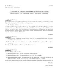
Example 2.36. If dimM = 3 and dimS = 2, then (TpS ∩ξp) ⊥ = TpS ∩ξp at the<br />
points p ∈ S where TpS ∩ ξp is 1–dimensional. Figure 2 shows the characteristic<br />
foliation of the unit 2–sphere in (R 3 , ξ2), where ξ2 denotes the standard contact<br />
26
structure of Example 2.7: The only singular points are (0, 0, ±1); away from these<br />
points the characteristic foliation is spanned by<br />
(y − xz)∂x − (x + yz)∂y + (x 2 + y 2 )∂z.<br />
Figure 2: The characteristic foliation on S 2 ⊂ (R 3 , ξ2).<br />
The following lemma helps to clarify the notion of singular 1–dimensional<br />
foliation.<br />
Lemma 2.37. Let β0 be the 1–form induced on S by a contact form α defining ξ,<br />
and let Ω be a volume form on S. Then Sξ is defined by the vector field X<br />
satisfying<br />
iXΩ = β0 ∧ (dβ0) n−1 .<br />
Proof. First of all, we observe that β0 ∧ (dβ0) n−1 �= 0 outside the zeros of β0:<br />
Arguing by contradiction, assume β0,p �= 0 and β0 ∧(dβ0) n−1 |p = 0 at some p ∈ S.<br />
Then (dβ0) n |p �= 0 by (2.5). On the codimension 1 subspace kerβ0,p of TpS the<br />
symplectic form dβ0,p has maximal rank n−1. It follows that β0 ∧(dβ0) n−1 |p �= 0<br />
after all, a contradiction.<br />
Next we want to show that X ∈ ker β0. We observe<br />
0 = iX(iXΩ) = β0(X)(dβ0) n−1 − (n − 1)β0 ∧ iXdβ0 ∧ (dβ0) n−2 . (2.6)<br />
Taking the exterior product of this equation with β0 we get<br />
β0(X)β0 ∧ (dβ0) n−1 = 0.<br />
By our previous consi<strong>der</strong>ation this implies β0(X) = 0.<br />
It remains to show that for β0,p �= 0 we have<br />
dβ0(X(p), v) = 0 for all v ∈ TpS ∩ ξp.<br />
27
For n = 1 this is trivially satisfied, because in that case v is a multiple of X(p).<br />
I suppress the point p in the following calculation, where we assume n ≥ 2.<br />
From (2.6) and with β0(X) = 0 we have<br />
Taking the interior product with v ∈ TS ∩ ξ yields<br />
β0 ∧ iXdβ0 ∧ (dβ0) n−2 = 0. (2.7)<br />
−dβ0(X, v)β0 ∧ (dβ0) n−2 + (n − 2)β0 ∧ iXdβ0 ∧ ivdβ0 ∧ (dβ0) n−3 = 0.<br />
(Thanks to the coefficient n − 2 the term (dβ0) n−3 is not a problem for n = 2.)<br />
Taking the exterior product of that last equation with dβ0, and using (2.7), we<br />
find<br />
and thus dβ0(X, v) = 0.<br />
dβ0(X, v)β0 ∧ (dβ0) n−1 = 0,<br />
Remark 2.38. (1) We can now give a more formal definition of ‘singular 1–<br />
dimensional foliation’ as an equivalence class of vector fields [X], where X is<br />
allowed to have zeros and [X] = [X ′ ] if there is a nowhere zero function on all<br />
of S such that X ′ = fX. Notice that the non-integrability of contact structures<br />
and the reasoning at the beginning of the proof of the lemma imply that the zero<br />
set of X does not contain any open subsets of S.<br />
(2) If the contact structure ξ is cooriented rather than just coorientable, so<br />
that α is well-defined up to multiplication with a positive function, then this<br />
lemma allows to give an orientation to the characteristic foliation: Changing α<br />
to λα with λ: M → R + will change β0 ∧ (dβ0) n−1 by a factor λ n .<br />
We now restrict attention to surfaces in contact 3–manifolds, where the notion<br />
of characteristic foliation has proved to be particularly useful.<br />
The following theorem is due to E. Giroux [52].<br />
Theorem 2.39 (Giroux). Let Si be closed surfaces in contact 3–manifolds (Mi, ξi),<br />
i = 0, 1 (with ξi coorientable), and φ: S0 → S1 a diffeomorphism with φ(S0,ξ0 ) =<br />
as oriented characteristic foliations. Then there is a contactomorphism<br />
S1,ξ1<br />
ψ: N(S0) → N(S1) of suitable neighbourhoods N(Si) of Si with ψ(S0) = S1<br />
and such that ψ|S0 is isotopic to φ via an isotopy preserving the characteristic<br />
foliation.<br />
28
Proof. By passing to a double cover, if necessary, we may assume that the Si<br />
are orientable hypersurfaces. Let αi be contact forms defining ξi. Extend φ to a<br />
diffeomorphism (still denoted φ) of neighbourhoods of Si and consi<strong>der</strong> the contact<br />
forms α0 and φ ∗ α1 on a neighbourhood of S0, which we may identify with S0 ×R.<br />
By rescaling α1 we may assume that α0 and φ ∗ α1 induce the same form β0<br />
on S0 ≡ S0 × {0}, and hence also the same form dβ0.<br />
Observe that the expression on the right-hand side of equation (2.5) is linear in<br />
˙βr and ur. This implies that convex linear combinations of solutions of (2.5) (for<br />
n = 1) with the same β0 (and dβ0) will again be solutions of (2.5) for sufficiently<br />
small r. This reasoning applies to<br />
αt := (1 − t)α0 + tφ ∗ α1, t ∈ [0, 1].<br />
(I hope the rea<strong>der</strong> will forgive the slight abuse of notation, with α1 denoting both<br />
a form on M1 and its pull-back φ ∗ α1 to M0.) As is to be expected, we now use<br />
the Moser trick to find an isotopy ψt with ψ ∗ t αt = λtα0, just as in the proof of<br />
Gray stability (Theorem 2.20). In particular, we require as there that the vector<br />
field Xt that we want to integrate to the flow ψt lie in the kernel of αt.<br />
On TS0 we have ˙αt ≡ 0 (thanks to the assumption that α0 and φ ∗ α1 induce<br />
the same form β0 on S0). In particular, if v is a vector in S0,ξ0 , then by equation<br />
(2.1) we have dαt(Xt, v) = 0, which implies that Xt is a multiple of v, hence<br />
tangent to S0,ξ0 . This shows that the flow of Xt preserves S0 and its characteristic<br />
foliation. More formally, we have<br />
LXtαt = d(αt(Xt)) + iXtdαt = iXtdαt,<br />
so with v as above we have LXtαt(v) = 0, which shows that LXtαt|TS0 is a<br />
multiple of α0|TS0 = β0. This implies that the (local) flow of Xt changes β0 by a<br />
conformal factor.<br />
Since S0 is closed, the local flow of Xt restricted to S0 integrates up to t = 1,<br />
and so the same is true 3 in a neighbourhood of S0. Then ψ = φ ◦ ψ1 will be the<br />
desired diffeomorphism N(S0) → N(S1).<br />
As observed previously in the proof of Darboux’s theorem for contact forms,<br />
the Moser trick allows more flexibility if we drop the condition αt(Xt) = 0.<br />
We are now going to exploit this extra freedom to strengthen Giroux’s theorem<br />
3 Cf. the proof (and the footnote therein) of Darboux’s theorem (Thm. 2.24).<br />
29
slightly. This will be important later on when we want to extend isotopies of<br />
hypersurfaces.<br />
Theorem 2.40. Un<strong>der</strong> the assumptions of the preceding theorem we can find<br />
ψ: N(S0) → N(S1) satisfying the stronger condition that ψ|S0 = φ.<br />
Proof. We want to show that the isotopy ψt of the preceding proof may be as-<br />
sumed to fix S0 pointwise. As there, we may assume ˙αt|TS0<br />
≡ 0.<br />
If the condition that Xt be tangent to kerαt is dropped, the condition Xt<br />
needs to satisfy so that its flow will pull back αt to λtα0 is<br />
˙αt + d(αt(Xt)) + iXtdαt = µtαt, (2.8)<br />
where µt and λt are related by µt = d<br />
dt (log λt) ◦ ψ −1<br />
t , cf. the proof of the Gray<br />
stability theorem (Theorem 2.20).<br />
Write Xt = HtRt+Yt with Rt the Reeb vector field of αt and Yt ∈ ξt = kerαt.<br />
Then condition (2.8) translates into<br />
˙αt + dHt + iYtdαt = µtαt. (2.9)<br />
For given Ht one determines µt from this equation by inserting the Reeb vector<br />
field Rt; the equation then admits a unique solution Yt ∈ kerαt because of the<br />
non-degeneracy of dαt|ξt .<br />
Our aim now is to ensure that Ht ≡ 0 on S0 and Yt ≡ 0 along S0. The latter<br />
we achieve by imposing the condition<br />
˙αt + dHt = 0 along S0<br />
(2.10)<br />
(which entails with (2.9) that µt|S0 ≡ 0). The conditions Ht ≡ 0 on S0 and (2.10)<br />
can be simultaneously satisfied thanks to ˙αt|TS0 ≡ 0.<br />
We can therefore find a smooth family of smooth functions Ht satisfying these<br />
conditions, and then define Yt by (2.9). The flow of the vector field Xt = HtRt+Yt<br />
then defines an isotopy ψt that fixes S0 pointwise (and thus is defined for all<br />
t ∈ [0, 1] in a neighbourhood of S0). Then ψ = φ ◦ ψ1 will be the diffeomorphism<br />
we wanted to construct.<br />
2.4.5 Applications<br />
Perhaps the most important consequence of the neighbourhood theorems proved<br />
above is that they allow us to perform differential topological constructions such<br />
30
as surgery or similar cutting and pasting operations in the presence of a contact<br />
structure, that is, these constructions can be carried out on a contact manifold<br />
in such a way that the resulting manifold again carries a contact structure.<br />
One such construction that I shall explain in detail in Section 3 is the surgery<br />
of contact 3–manifolds along transverse knots, which enables us to construct a<br />
contact structure on every closed, orientable 3–manifold.<br />
The concept of characteristic foliation on surfaces in contact 3–manifolds<br />
has proved seminal for the classification of contact structures on 3–manifolds,<br />
although it has recently been superseded by the notion of dividing curves. It is<br />
clear that Theorem 2.39 can be used to cut and paste contact manifolds along<br />
hypersurfaces with the same characteristic foliation. What actually makes this<br />
useful in dimension 3 is that there are ways to manipulate the characteristic<br />
foliation of a surface by isotoping that surface inside the contact 3–manifold.<br />
The most important result in that direction is the Elimination Lemma proved<br />
by Giroux [52]; an improved version is due to D. Fuchs, see [26]. This lemma<br />
says that un<strong>der</strong> suitable assumptions it is possible to cancel singular points of the<br />
characteristic foliation in pairs by a C 0 –small isotopy of the surface (specifically:<br />
an elliptic and a hyperbolic point of the same sign – the sign being determined<br />
by the matching or non-matching of the orientation of the surface S and the<br />
contact structure ξ at the singular point of Sξ). For instance, Eliashberg [24] has<br />
shown that if a contact 3–manifold (M, ξ) contains an embedded disc D ′ such<br />
that D ′ ξ<br />
has a limit cycle, then one can actually find a so-called overtwisted disc:<br />
an embedded disc D with boundary ∂D tangent to ξ (but D transverse to ξ<br />
along ∂D, i.e. no singular points of Dξ on ∂D) and with Dξ having exactly one<br />
singular point (of elliptic type); see Section 3.6.<br />
Moreover, in the generic situation it is possible, given surfaces S ⊂ (M, ξ)<br />
and S ′ ⊂ (M ′ , ξ ′ ) with Sξ homeomorphic to S ′ ξ ′, to perturb one of the surfaces so<br />
as to get diffeomorphic characteristic foliations.<br />
Chapter 8 of [1] contains a section on surfaces in contact 3–manifolds, and<br />
in particular a proof of the Elimination Lemma. Further introductory reading<br />
on the matter can be found in the lectures of J. Etnyre [35]; of the sources cited<br />
above I recommend [26] as a starting point.<br />
In [52] Giroux initiated the study of convex surfaces in contact 3–manifolds.<br />
These are surfaces S with an infinitesimal automorphism X of the contact struc-<br />
ture ξ with X transverse to S. For such surfaces, it turns out, much less infor-<br />
31
mation than the characteristic foliation Sξ is needed to determine ξ in a neigh-<br />
bourhood of S, viz., only the so-called dividing set of Sξ. This notion lies at the<br />
centre of most of the recent advances in the classification of contact structures<br />
on 3–manifolds [55], [71], [72]. A brief introduction to convex surface theory can<br />
be found in [35].<br />
2.5 Isotopy extension theorems<br />
In this section we show that the isotopy extension theorem of differential topology<br />
– an isotopy of a closed submanifold extends to an isotopy of the ambient manifold<br />
– remains valid for the various distinguished submanifolds of contact manifolds.<br />
The neighbourhood theorems proved above provide the key to the corresponding<br />
isotopy extension theorems. For simplicity, I assume throughout that the ambient<br />
contact manifold M is closed; all isotopy extension theorems remain valid if M has<br />
non-empty boundary ∂M, provided the isotopy stays away from the boundary.<br />
In that case, the isotopy of M found by extension keeps a neighbourhood of<br />
∂M fixed. A further convention throughout is that our ambient isotopies ψt are<br />
un<strong>der</strong>stood to start at ψ0 = idM.<br />
2.5.1 Isotropic submanifolds<br />
An embedding j : L → (M, ξ = kerα) is called isotropic if j(L) is an isotropic<br />
submanifold of (M, ξ), i.e. everywhere tangent to the contact structure ξ. Equiv-<br />
alently, one needs to require j ∗ α ≡ 0.<br />
Theorem 2.41. Let jt: L → (M, ξ = kerα), t ∈ [0, 1], be an isotopy of isotropic<br />
embeddings of a closed manifold L in a contact manifold (M, ξ). Then there is a<br />
compactly supported contact isotopy ψt: M → M with ψt(j0(L)) = jt(L).<br />
Proof. Define a time-dependent vector field Xt along jt(L) by<br />
Xt ◦ jt = d<br />
dt jt.<br />
To simplify notation later on, we assume that L is a submanifold of M and j0 the<br />
inclusion L ⊂ M. Our aim is to find a (smooth) family of compactly supported,<br />
smooth functions � Ht: M → R whose Hamiltonian vector field � Xt equals Xt along<br />
jt(L). Recall that � Xt is defined in terms of � Ht by<br />
α( � Xt) = � Ht, i�Xt dα = d � Ht(Rα)α − d � Ht,<br />
32
where, as usual, Rα denotes the Reeb vector field of α.<br />
Hence, we need<br />
α(Xt) = � Ht, iXtdα = d � Ht(Rα)α − d � Ht along jt(L). (2.11)<br />
Write Xt = HtRα + Yt with Ht: jt(L) → R and Yt ∈ kerα. To satisfy (2.11) we<br />
need<br />
This implies<br />
�Ht = Ht along jt(L). (2.12)<br />
d � Ht(v) = dHt(v) for v ∈ T(jt(L)).<br />
Since jt is an isotopy of isotropic embeddings, we have T(jt(L)) ⊂ ker α. So a<br />
prerequisite for (2.11) is that<br />
We have<br />
dα(Xt, v) = −dHt(v) for v ∈ T(jt(L)). (2.13)<br />
dα(Xt, v) + dHt(v) = dα(Xt, v) + d(α(Xt))(v)<br />
so equation (2.13) is equivalent to<br />
= iv(iXtdα + d(iXtα))<br />
= iv(LXtα),<br />
iv(LXtα) = 0 for v ∈ T(jt(L)).<br />
But this is indeed tautologically satisfied: The fact that jt is an isotopy of isotropic<br />
embeddings can be written as j ∗ t α ≡ 0; this in turn implies 0 = d<br />
dt (j∗ t α) =<br />
j ∗ t (LXtα), as desired.<br />
This means that we can define � Ht by prescribing the value of � Ht along jt(L)<br />
(with (2.12)) and the differential of � Ht along jt(L) (with (2.11)), where we are<br />
free to impose d � Ht(Rα) = 0, for instance. The calculation we just performed<br />
shows that these two requirements are consistent with each other. Any function<br />
satisfying these requirements along jt(L) can be smoothed out to zero outside a<br />
tubular neighbourhood of jt(L), and the Hamiltonian flow of this � Ht will be the<br />
desired contact isotopy extending jt.<br />
One small technical point is to ensure that the resulting family of functions<br />
�Ht will be smooth in t. To achieve this, we proceed as follows. Set ˆ M = M ×[0, 1]<br />
and<br />
ˆL = �<br />
q∈L,t∈[0,1]<br />
33<br />
(jt(q), t),
so that ˆ L is a submanifold of ˆ M. Let g be an auxiliary Riemannian metric on M<br />
with respect to which Rα is orthogonal to kerα. Identify the normal bundle N ˆ L<br />
of ˆ L in ˆ M with a sub-bundle of T ˆ M by requiring its fibre at a point (p, t) ∈ ˆ L<br />
to be the g–orthogonal subspace of Tp(jt(L)) in TpM. Let τ : N ˆ L → ˆ M be a<br />
tubular map.<br />
Now define a smooth function ˆ H : N ˆ L → R as follows, where (p, t) always<br />
denotes a point of ˆ L ⊂ N ˆ L.<br />
• ˆ H(p, t) = α(Xt),<br />
• d ˆ H (p,t)(Rα) = 0,<br />
• d ˆ H (p,t)(v) = −dα(Xt, v) for v ∈ kerαp ⊂ TpM ⊂ T (p,t) ˆ M,<br />
• ˆ H is linear on the fibres of N ˆ L → ˆ L.<br />
Let χ: ˆ M → [0, 1] be a smooth function with χ ≡ 0 outside a small neighbour-<br />
hood N0 ⊂ τ(N ˆ L) of ˆ L and χ ≡ 1 in a smaller neighbourhood N1 ⊂ N0 of ˆ L.<br />
For (p, t) ∈ ˆ M, set<br />
�Ht(p) =<br />
�<br />
χ(p, t) ˆ H(τ −1 (p, t)) for (p, t) ∈ τ(N ˆ L)<br />
0 for (p, t) �∈ τ(N ˆ L).<br />
This is smooth in p and t, and the Hamiltonian flow ψt of � Ht (defined globally<br />
since � Ht is compactly supported) is the desired contact isotopy.<br />
2.5.2 <strong>Contact</strong> submanifolds<br />
An embedding j : (M ′ , ξ ′ ) → (M, ξ) is called a contact embedding if<br />
is a contact submanifold of (M, ξ), i.e.<br />
(j(M ′ ), Tj(ξ ′ ))<br />
T(j(M)) ∩ ξ| j(M) = Tj(ξ ′ ).<br />
If ξ = kerα, this can be reformulated as kerj ∗ α = ξ ′ .<br />
Theorem 2.42. Let jt: (M ′ , ξ ′ ) → (M, ξ), t ∈ [0, 1], be an isotopy of con-<br />
tact embeddings of the closed contact manifold (M ′ , ξ ′ ) in the contact manifold<br />
(M, ξ). Then there is a compactly supported contact isotopy ψt: M → M with<br />
ψt(j0(M ′ )) = jt(M ′ ).<br />
34
Proof. In the proof of this theorem we follow a slightly different strategy from<br />
the one in the isotropic case. Instead of directly finding an extension of the<br />
Hamiltonian Ht: jt(M ′ ) → R, we first use the neighbourhood theorem for con-<br />
tact submanifolds to extend jt to an isotopy of contact embeddings of tubular<br />
neighbourhoods.<br />
Again we assume that M ′ is a submanifold of M and j0 the inclusion M ′ ⊂ M.<br />
As earlier, NM ′ denotes the normal bundle of M ′ in M. We also identify M ′<br />
with the zero section of NM ′ , and we use the canonical identification<br />
T(NM ′ )|M ′ = TM ′ ⊕ NM ′ .<br />
By the usual isotopy extension theorem from differential topology we find an<br />
isotopy<br />
φt: NM ′ −→ M<br />
with φt|M ′ = jt.<br />
Choose contact forms α, α ′ defining ξ and ξ ′ , respectively. Define αt = φ∗ tα.<br />
Then TM ′ ∩ kerαt = ξ ′ . Let R ′ denote the Reeb vector field of α ′ . Analogous<br />
to the proof of Theorem 2.32, we first find a smooth family of smooth functions<br />
gt: M ′ → R + such that gtαt|TM ′ = α′ , and then a family ft: NM ′ → R + with<br />
ft|M ′ ≡ 1 and<br />
dft = iR ′d(gtαt) on T(NM ′ )|M ′.<br />
Then βt = ftgtαt is a family of contact forms on NM ′ representing the contact<br />
structure ker(φ ∗ tα) and with the properties<br />
βt|TM ′ = α′ ,<br />
dβt|TM ′ = dα′ ,<br />
ker(dβt) = 〈R ′ 〉 along M ′ .<br />
The family (NM ′ , dβt) of symplectic vector bundles may be thought of as a<br />
symplectic vector bundle over M ′ × [0, 1], which is necessarily isomorphic to a<br />
bundle pulled back from M ′ × {0} (cf. [74, Cor. 3.4.4]). In other words, there is<br />
a smooth family of symplectic bundle isomorphisms<br />
Then<br />
Φt: (NM ′ , dβ0) −→ (NM ′ , dβt).<br />
idTM ′ ⊕ Φt: T(NM ′ )|M ′ −→ T(NM′ )|M ′<br />
35
is a bundle map that pulls back βt to β0 and dβt to dβ0.<br />
By the now familiar stability argument we find a smooth family of embeddings<br />
ϕt: N(M ′ ) −→ NM ′<br />
for some neighbourhood N(M ′ ) of the zero section M ′ in NM ′ with ϕ0 =<br />
inclusion, ϕt|M ′ = idM ′ and ϕ∗ tβt = λtβ0, where λt: N(M ′ ) → R + . This means<br />
that<br />
φt ◦ ϕt: N(M ′ ) −→ M<br />
is a smooth family of contact embeddings of (N(M ′ ), ker β0) in (M, ξ).<br />
Define a time-dependent vector field Xt along φt ◦ ϕt(N(M ′ )) by<br />
Xt ◦ φt ◦ ϕt = d<br />
dt (φt ◦ ϕt).<br />
This Xt is clearly an infinitesimal automorphism of ξ: By differentiating the<br />
equation ϕ ∗ tφ ∗ tα = µtφ ∗ 0 α (where µt: N(M ′ ) → R + ) with respect to t we get<br />
ϕ ∗ tφ ∗ t(LXtα) = ˙µtφ ∗ 0α = ˙µt<br />
ϕ ∗ tφ ∗ tα,<br />
so LXtα is a multiple of α (since φt ◦ ϕt is a diffeomorphism onto its image).<br />
By the theory of contact Hamiltonians, Xt is the Hamiltonian vector field of<br />
a Hamiltonian function ˆ Ht defined on φt ◦ ϕt(N(M ′ )). Cut off this function with<br />
a bump function so as to obtain Ht: M → R with Ht ≡ ˆ Ht near φt ◦ ϕt(M ′ )<br />
and Ht ≡ 0 outside a slightly larger neighbourhood of φt ◦ ϕt(M ′ ). Then the<br />
Hamiltonian flow ψt of Ht satisfies our requirements.<br />
2.5.3 Surfaces in 3–manifolds<br />
Theorem 2.43. Let jt: S → (M, ξ = kerα), t ∈ [0, 1], be an isotopy of embed-<br />
dings of a closed surface S in a 3–dimensional contact manifold (M, ξ). If all jt<br />
induce the same characteristic foliation on S, then there is a compactly supported<br />
isotopy ψt: M → M with ψt(j0(S)) = jt(S).<br />
Proof. Extend jt to a smooth family of embeddings φt: S ×R → M, and identify<br />
S with S × {0}. The assumptions say that all φ ∗ tα induce the same characteristic<br />
foliation on S. By the proof of Theorem 2.40 and in analogy with the proof of<br />
Theorem 2.42 we find a smooth family of embeddings<br />
µt<br />
ϕt: S × (−ε, ε) −→ S × R<br />
36
for some ε > 0 with ϕ0 = inclusion, ϕt| S×{0} = idS and ϕ∗ tφ∗ tα = λtφ∗ 0α, where<br />
λt: S × (−ε, ε) → R + . In other words, φt ◦ ϕt is a smooth family of contact<br />
embeddings of (S × (−ε, ε), ker φ∗ 0α) in (M, ξ).<br />
The proof now concludes exactly as the proof of Theorem 2.42.<br />
2.6 Approximation theorems<br />
A further manifestation of the (local) flexibility of contact structures is the fact<br />
that a given submanifold can, un<strong>der</strong> fairly weak (and usually obvious) topological<br />
conditions, be approximated (typically C 0 –closely) by a contact submanifold or<br />
an isotropic submanifold, respectively. The most general results in this direction<br />
are best phrased in M. Gromov’s language of h-principles. For a recent text on<br />
h-principles that puts particular emphasis on symplectic and contact geometry<br />
see [30]; a brief and perhaps more gentle introduction to h-principles can be found<br />
in [47].<br />
In the present section I restrict attention to the 3–dimensional situation, where<br />
the relevant approximation theorems can be proved by elementary geometric ad<br />
hoc techniques.<br />
Theorem 2.44. Let γ : S 1 → (M, ξ) be a knot, i.e. an embedding of S 1 , in<br />
a contact 3–manifold. Then γ can be C 0 –approximated by a Legendrian knot<br />
isotopic to γ. Alternatively, it can be C 0 –approximated by a positively as well as<br />
a negatively transverse knot.<br />
In or<strong>der</strong> to prove this theorem, we first consi<strong>der</strong> embeddings γ : (a, b) →<br />
(R 3 , ξ) of an open interval in R 3 with its standard contact structure ξ = kerα,<br />
where α = dz + x dy. Write γ(t) = (x(t), y(t), z(t)). Then<br />
α(˙γ) = ˙z + x ˙y,<br />
so the condition for a Legendrian curve reads ˙z + x ˙y ≡ 0; for a positively (resp.<br />
negatively) transverse curve, ˙z + x ˙y > 0 (resp. < 0).<br />
There are two ways to visualise such curves. The first is via its front pro-<br />
jection<br />
γF(t) = (y(t), z(t)),<br />
the second via its Lagrangian projection<br />
γL(t) = (x(t), y(t)).<br />
37
2.6.1 Legendrian knots<br />
If γ(t) = (x(t), y(t), z(t)) is a Legendrian curve in R 3 , then ˙y = 0 implies ˙z = 0,<br />
so there the front projection has a singular point. Indeed, the curve t ↦→ (t, 0, 0)<br />
is an example of a Legendrian curve whose front projection is a single point. We<br />
call a Legendrian curve generic if ˙y = 0 only holds at isolated points (which we<br />
call cusp points), and there ¨y �= 0.<br />
Lemma 2.45. Let γ : (a, b) → (R 3 , ξ) be a Legendrian immersion. Then its front<br />
projection γF(t) = (y(t), z(t)) does not have any vertical tangencies. Away from<br />
the cusp points, γ is recovered from its front projection via<br />
x(t) = − ˙z(t)<br />
= −dz<br />
˙y(t) dy ,<br />
i.e. x(t) is the negative slope of the front projection. The curve γ is embedded if<br />
and only if γF has only transverse self-intersections.<br />
By a C ∞ –small perturbation of γ we can obtain a generic Legendrian curve ˜γ<br />
isotopic to γ; by a C 2 –small perturbation we may achieve that the front projection<br />
has only semi-cubical cusp singularities, i.e. around a cusp point at t = 0 the curve<br />
˜γ looks like<br />
with λ �= 0, see Figure 3.<br />
˜γ(t) = (t + a, λt 2 + b, −λ(2t 3 /3 + at 2 ) + c)<br />
Any regular curve in the (y, z)–plane with semi-cubical cusps and no vertical<br />
tangencies can be lifted to a unique Legendrian curve in R 3 .<br />
Figure 3: The cusp of a front projection.<br />
Proof. The Legendrian condition is ˙z + x ˙y = 0. Hence ˙y = 0 forces ˙z = 0, so γF<br />
cannot have any vertical tangencies.<br />
Away from the cusp points, the Legendrian condition tells us how to recover<br />
x as the negative slope of the front projection. (By continuity, the equation<br />
38
x = dz<br />
dy<br />
also makes sense at generic cusp points.) In particular, a self-intersecting<br />
front projection lifts to a non-intersecting curve if and only if the slopes at the<br />
intersection point are different, i.e. if and only if the intersection is transverse.<br />
That γ can be approximated in the C ∞ –topology by a generic immersion<br />
˜γ follows from the usual transversality theorem (in its most simple form, viz.,<br />
applied to the function y(t); the function x(t) may be left unchanged, and the<br />
new z(t) is then found by integrating the new −x ˙y).<br />
At a cusp point of ˜γ we have ˙y = ˙z = 0. Since ˜γ is an immersion, this forces<br />
˙x �= 0, so ˜γ can be parametrised around a cusp point by the x–coordinate, i.e. we<br />
may choose the curve parameter t such that the cusp lies at t = 0 and x(t) = t+a.<br />
Since ¨y(0) �= 0 by the genericity condition, we can write y(t) = t 2 g(t) + y(0)<br />
with a smooth function g(t) satisfying g(0) �= 0 (This is proved like the ‘Morse<br />
lemma’ in Appendix 2 of [77]). A C 0 –approximation of g(t) by a function h(t)<br />
with h(t) ≡ g(0) for t near zero and h(t) ≡ g(t) for |t| greater than some small<br />
ε > 0 yields a C 2 –approximation of y(t) with the desired form around the cusp<br />
point.<br />
Example 2.46. Figure 4 shows the front projection of a Legendrian trefoil knot.<br />
Figure 4: Front projection of a Legendrian trefoil knot.<br />
Proof of Theorem 2.44 - Legendrian case. First of all, we consi<strong>der</strong> a curve γ in<br />
standard R 3 . In or<strong>der</strong> to find a C 0 –close approximation of γ, we simply need<br />
to choose a C 0 –close approximation of its front projection γF by a regular curve<br />
without vertical tangencies and with isolated cusps (we call such a curve a front)<br />
39
in such a way, that the slope of the front at time t is close to −x(t) (see Figure 5).<br />
Then the Legendrian lift of this front is the desired C 0 –approximation of γ.<br />
z<br />
Figure 5: Legendrian C 0 –approximation via front projection.<br />
If γ is defined on an interval (a, b) and is already Legendrian near its endpoints,<br />
then the approximation of γF may be assumed to coincide with γF near the<br />
endpoints, so that the Legendrian lift coincides with γ near the endpoints.<br />
Hence, given a knot in an arbitrary contact 3–manifold, we can cut it (by the<br />
Lebesgue lemma) into little pieces that lie in Darboux charts. There we can use<br />
the preceding recipe to find a Legendrian approximation. Since, as just observed,<br />
one can find such approximations on intervals with given boundary condition,<br />
this procedure yields a Legendrian approximation of the full knot.<br />
Locally (i.e. in R 3 ) the described procedure does not introduce any self-<br />
intersections in the approximating curve, provided we approximate γF by a front<br />
with only transverse self-intersections. Since the original knot was embedded, the<br />
same will then be true for its Legendrian C 0 –approximation.<br />
The same result may be <strong>der</strong>ived using the Lagrangian projection:<br />
Lemma 2.47. Let γ : (a, b) → (R 3 , ξ) be a Legendrian immersion. Then its<br />
Lagrangian projection γL(t) = (x(t), y(t)) is also an immersed curve. The curve<br />
γ is recovered from γL via<br />
� t1<br />
z(t1) = z(t0) −<br />
40<br />
t0<br />
x dy.<br />
y
A Legendrian immersion γ : S 1 → (R 3 , ξ) has a Lagrangian projection that en-<br />
closes zero area. Moreover, γ is embedded if and only if every loop in γL (except,<br />
in the closed case, the full loop γL) encloses a non-zero oriented area.<br />
Any immersed curve in the (x, y)–plane is the Lagrangian projection of a<br />
Legendrian curve in R 3 , unique up to translation in the z–direction.<br />
Proof. The Legendrian condition ˙z + x ˙y implies that if ˙y = 0 then ˙z = 0, and<br />
hence, since γ is an immersion, ˙x �= 0. So γL is an immersion.<br />
The formula for z follows by integrating the Legendrian condition. For a<br />
closed curve γL in the (x, y)–plane, the integral �<br />
x dy computes the oriented<br />
area enclosed by γL. From that all the other statements follow.<br />
Example 2.48. Figure 6 shows the Lagrangian projection of a Legendrian un-<br />
knot.<br />
A −2A<br />
Figure 6: Lagrangian projection of a Legendrian unknot.<br />
Alternative proof of Theorem 2.44 – Legendrian case. Again we consi<strong>der</strong> a curve<br />
γ in standard R 3 defined on an interval. The generalisation to arbitrary contact<br />
manifolds and closed curves is achieved as in the proof using front projections.<br />
In or<strong>der</strong> to find a C 0 –approximation of γ by a Legendrian curve, one only has<br />
to approximate its Lagrangian projection γL by an immersed curve whose ‘area<br />
integral’<br />
z(t0) −<br />
lies as close to the original z(t) as one wishes. This can be achieved by using small<br />
loops oriented positively or negatively (see Figure 7). If γL has self-intersections,<br />
this approximating curve can be chosen in such a way that along loops properly<br />
contained in that curve the area integral is non-zero, so that again we do not<br />
� t<br />
t0<br />
x dy<br />
introduce any self-intersections in the Legendrian approximation of γ.<br />
41<br />
γL<br />
A
y<br />
Figure 7: Legendrian C 0 –approximation via Lagrangian projection.<br />
2.6.2 Transverse knots<br />
The quickest proof of the transverse case of Theorem 2.44 is via the Legendrian<br />
case. However, it is perfectly feasible to give a direct proof along the lines of the<br />
preceding discussion, i.e. using the front or the Lagrangian projection. Since this<br />
picture is useful elsewhere, I include a brief discussion, restricting attention to<br />
the front projection.<br />
Thus, let γ(t) = (x(t), y(t), z(t)) be a curve in R 3 . The condition for γ to be<br />
positively transverse to the standard contact structure ξ = ker(dz + x dy) is that<br />
˙z + x ˙y > 0. Hence,<br />
⎧<br />
⎪⎨<br />
⎪⎩<br />
if ˙y = 0, then ˙z > 0,<br />
if ˙y > 0, then x > − ˙z/ ˙y,<br />
if ˙y < 0, then x < − ˙z/ ˙y.<br />
The first statement says that there are no vertical tangencies oriented down-<br />
wards in the front projection. The second statement says in particular that for<br />
˙y > 0 and ˙z < 0 we have x > 0; the third, that for ˙y < 0 and ˙z < 0 we have<br />
x < 0. This implies that the situations shown in Figure 8 are not possible in the<br />
front projection of a positively transverse curve. I leave it to the rea<strong>der</strong> to check<br />
that all other oriented crossings are possible in the front projection of a positively<br />
transverse curve, and that any curve in the (y, z)–plane without the forbidden<br />
crossing or downward vertical tangencies admits a lift to a positively transverse<br />
curve.<br />
42<br />
x
Figure 8: Impossible front projections of positively transverse curve.<br />
Example 2.49. Figure 9 shows the front projection of a positively transverse<br />
trefoil knot.<br />
Figure 9: Front projection of a positively transverse trefoil knot.<br />
Proof of Theorem 2.44 – transverse case. By the Legendrian case of this theo-<br />
rem, the given knot γ can be C 0 –approximated by a Legendrian knot γ1. By<br />
Example 2.29, a neighbourhood of γ1 in (M, ξ) looks like a solid torus S 1 × D 2<br />
with contact structure cosθ dx − sinθ dy = 0, where γ1 ≡ S 1 × {0}. Then the<br />
curve<br />
γ2(t) = (θ = t, x = δ sint, y = δ cos t), t ∈ [0, 2π],<br />
is a positively (resp. negatively) transverse knot if δ > 0 (resp. < 0). By choosing<br />
|δ| small we obtain as good a C 0 –approximation of γ1 and hence of γ as we<br />
wish.<br />
3 <strong>Contact</strong> structures on 3–manifolds<br />
Here is the main theorem proved in this section:<br />
43
Theorem 3.1 (Lutz-Martinet). Every closed, orientable 3–manifold admits a<br />
contact structure in each homotopy class of tangent 2–plane fields.<br />
In Section 3.2 I present what is essentially J. Martinet’s [90] proof of the<br />
existence of a contact structure on every 3–manifold. This construction is based<br />
on a surgery description of 3–manifolds due to R. Lickorish and A. Wallace. For<br />
the key step, showing how to extend over a solid torus certain contact forms<br />
defined near the boundary of that torus (which then makes it possible to perform<br />
Dehn surgeries), we use an approach due to W. Thurston and H. Winkelnkemper;<br />
this allows to simplify Martinet’s proof slightly.<br />
In Section 3.3 we show that every orientable 3–manifold is parallelisable and<br />
then build on this to classify (co-)oriented tangent 2–plane fields up to homotopy.<br />
In Section 3.4 we study the so-called Lutz twist, a topologically trivial Dehn<br />
surgery on a contact manifold (M, ξ) which yields a contact structure ξ ′ on M<br />
that is not homotopic (as 2–plane field) to ξ. We then complete the proof of the<br />
main theorem stated above. These results are contained in R. Lutz’s thesis [84]<br />
(which, I have to admit, I’ve never seen). Of Lutz’s published work, [83] only deals<br />
with the 3–sphere (and is only an announcement); [85] also deals with a more<br />
restricted problem. I learned the key steps of the construction from an exposition<br />
given in V. Ginzburg’s thesis [50]. I have added proofs of many topological details<br />
that do not seem to have appeared in a readily accessible source before.<br />
In Section 3.5 I indicate two further proofs for the existence of contact struc-<br />
tures on every 3–manifold (and provide references to others). The one by Thur-<br />
ston and Winkelnkemper uses a description of 3–manifolds as open books due to<br />
J. Alexan<strong>der</strong>; the crucial idea in their proof is the one we also use to simplify<br />
Martinet’s argument. Indeed, my discussion of the Lutz twist in the present<br />
section owes more to the paper by Thurston-Winkelnkemper than to any other<br />
reference. The second proof, by J. Gonzalo, is based on a branched cover descrip-<br />
tion of 3–manifolds found by H. Hilden, J. Montesinos and T. Thickstun. This<br />
branched cover description also yields a very simple geometric proof that every<br />
orientable 3–manifold is parallelisable.<br />
In Section 3.6 we discuss the fundamental dichotomy between tight and over-<br />
twisted contact structures, introduced by Eliashberg, as well as the relation of<br />
these types of contact structures with the concept of symplectic fillability. The<br />
chapter concludes in Section 3.7 with a survey of classification results for contact<br />
structures on 3–manifolds.<br />
44
But first we discuss, in Section 3.1, an invariant of transverse knots in R 3<br />
with its standard contact structure. This invariant will be an ingredient in the<br />
proof of the Lutz-Martinet theorem, but is also of independent interest.<br />
I do not feel embarrassed to use quite a bit of machinery from algebraic and<br />
differential topology in this chapter. However, I believe that nothing that cannot<br />
be found in such standard texts as [14], [77] and [95] is used without proof or an<br />
explicit reference.<br />
Throughout this third section, M denotes a closed, orientable 3-manifold.<br />
3.1 An invariant of transverse knots<br />
Although the invariant in question can be defined for transverse knots in arbitrary<br />
contact manifolds (provided the knot is homologically trivial), for the sake of<br />
clarity I restrict attention to transverse knots in R 3 with its standard contact<br />
structure ξ0 = ker(dz + x dy). This will be sufficient for the proof of the Lutz-<br />
Martinet theorem. In Section 3.7 I say a few words about the general situation<br />
and related invariants for Legendrian knots.<br />
Thus, let γ be a transverse knot in (R 3 , ξ0). Push γ a little in the direction<br />
of ∂x – notice that this is a nowhere zero vector field contained in ξ0, and in<br />
particular transverse to γ – to obtain a knot γ ′ . An orientation of γ induces an<br />
orientation of γ ′ . The orientation of R 3 is given by dx ∧ dy ∧ dz.<br />
Definition 3.2. The self-linking number l(γ) of the transverse knot γ is the<br />
linking number of γ and γ ′ .<br />
Notice that this definition is independent of the choice of orientation of γ (but<br />
it changes sign if the orientation of R 3 is reversed). Furthermore, in place of ∂x<br />
we could have chosen any nowhere zero vector field X in ξ0 to define l(γ): The<br />
difference between the the self-linking number defined via ∂x and that defined<br />
via X is the degree of the map γ → S 1 given by associating to a point on γ<br />
the angle between ∂x and X. This degree is computed with the induced map<br />
Z ∼ = H1(γ) → H1(S 1 ) ∼ = Z. But the map γ → S 1 factors through R 3 , so the<br />
induced homomorphism on homology is the zero homomorphism.<br />
Observe that l(γ) is an invariant un<strong>der</strong> isotopies of γ within the class of<br />
transverse knots.<br />
We now want to compute l(γ) from the front projection of γ. Recall that the<br />
writhe of an oriented knot diagram is the signed number of self-crossings of the<br />
45
diagram, where the sign of the crossing is given in Figure 10.<br />
−1<br />
+1<br />
Figure 10: Signs of crossings in a knot diagram.<br />
Lemma 3.3. The self-linking number l(γ) of a transverse knot is equal to the<br />
writhe w(γ) of its front projection.<br />
Proof. Let γ ′ be the push-off of γ as described. Observe that each crossing of the<br />
front projection of γ contributes a crossing of γ ′ un<strong>der</strong>neath γ of the corresponding<br />
sign. Since the linking number of γ and γ ′ is equal to the signed number of times<br />
that γ ′ crosses un<strong>der</strong>neath γ (cf. [98, p. 37]), we find that this linking number is<br />
equal to the signed number of self-crossings of γ, that is, l(γ) = w(γ).<br />
Proposition 3.4. Every self-linking number is realised by a transverse link in<br />
standard R 3 .<br />
Proof. Figure 11 shows front projections of positively transverse knots (cf. Sec-<br />
tion 2.6.2) with self-linking number ±3. From that the construction principle for<br />
realising any odd integer should be clear. With a two component link any even<br />
integer can be realised.<br />
Remark 3.5. It is no accident that I do not give an example of a transverse<br />
knot with even self-linking number. By a theorem of Eliashberg [26, Prop. 2.3.1]<br />
that relates l(γ) to the Euler characteristic of a Seifert surface S for γ and the<br />
signed number of singular points of the characteristic foliation Sξ, the self-linking<br />
number l(γ) of a knot can only take odd values.<br />
3.2 Martinet’s construction<br />
According to Lickorish [81] and Wallace [103] M can be obtained from S 3 by<br />
Dehn surgery along a link of 1–spheres. This means that we have to remove<br />
46
−3<br />
+3<br />
Figure 11: Transverse knots with self-linking number ±3.<br />
a disjoint set of embedded solid tori S 1 × D 2 from S 3 and glue back solid tori<br />
with suitable identification by a diffeomorphism along the boundaries S 1 × S 1 .<br />
The effect of such a surgery (up to diffeomorphism of the resulting manifold) is<br />
completely determined by the induced map in homology<br />
H1(S 1 × ∂D 2 ) −→ H1(S 1 × ∂D 2 )<br />
Z ⊕ Z −→ Z ⊕ Z,<br />
� �<br />
which is given by a unimodular matrix<br />
n q<br />
m p<br />
∈ GL(2, Z). Hence, denoting<br />
coordinates in S 1 × S 1 by (θ, ϕ), we may always assume the identification maps<br />
to be of the form �<br />
θ<br />
ϕ<br />
�<br />
↦−→<br />
�<br />
n q<br />
m p<br />
The curves µ and λ on ∂(S 1 × D 2 ) given respectively by θ = 0 and ϕ = 0 are<br />
called meridian and longitude. We keep the same notation µ, λ for the homology<br />
classes these curves represent. It turns out that the diffeomorphism type of the<br />
surgered manifold is completely determined by the class pµ + qλ, which is the<br />
class of the curve that becomes homotopically trivial in the surgered manifold<br />
(cf. [98, p. 28]). In fact, the Dehn surgery is completely determined by the surgery<br />
coefficient p/q, since the diffeomorphism of ∂(S 1 ×D 2 ) given by (λ, µ) ↦→ (λ, −µ)<br />
��<br />
extends to a diffeomorphism of the solid torus that we glue back.<br />
Similarly, the diffeomorphism given by (λ, µ) ↦→ (λ + kµ, µ) extends. By such<br />
a change of longitude in S 1 × D 2 ⊂ M, which amounts to choosing a different<br />
47<br />
θ<br />
ϕ<br />
�<br />
.
trivialisation of the normal bundle (i.e. framing) of S1 �<br />
�<br />
×{0} ⊂ M, the gluing map<br />
is changed to<br />
n q<br />
m − kn p − kq<br />
. By a change of longitude in the solid torus<br />
� �<br />
that we glue back, the gluing map is changed to<br />
n + kq q<br />
m + kp p<br />
. Thus, a Dehn<br />
surgery is a so-called handle surgery (or ‘honest surgery’ or simply ‘surgery’) if<br />
and only if the surgery coefficient � is �an<br />
integer, � that � is, q = ±1. For in exactly<br />
this case we may assume<br />
n q<br />
m p<br />
=<br />
0 1<br />
1 0<br />
, and the surgery is given by<br />
cutting out S 1 × D 2 and gluing back S 1 × D 2 with the identity map<br />
∂(D 2 × S 1 ) −→ ∂(S 1 × D 2 ).<br />
The theorem of Lickorish and Wallace remains true if we only allow handle<br />
surgeries. However, this assumption does not entail any great simplification of<br />
the existence proof for contact structures, so we shall work with general Dehn<br />
surgeries.<br />
Our aim in this section is to use this topological description of 3–manifolds<br />
for a proof of the following theorem, first proved by Martinet [90]. The proof<br />
presented here is in spirit the one given by Martinet, but, as indicated in the<br />
introduction to this third section, amalgamated with ideas of Thurston and<br />
Winkelnkemper [101], whose proof of the same theorem we shall discuss later.<br />
Theorem 3.6 (Martinet). Every closed, orientable 3–manifold M admits a con-<br />
tact structure.<br />
In view of the theorem of Lickorish and Wallace and the fact that S 3 admits<br />
a contact structure, Martinet’s theorem is a direct consequence of the following<br />
result.<br />
Theorem 3.7. Let ξ0 be a contact structure on a 3–manifold M0. Let M be the<br />
manifold obtained from M0 by a Dehn surgery along a knot K. Then M admits a<br />
contact structure ξ which coincides with ξ0 outside the neighbourhood of K where<br />
we perform surgery.<br />
Proof. By Theorem 2.44 we may assume that K is positively transverse to ξ0.<br />
Then, by the contact neighbourhood theorem (Example 2.33), we can find a<br />
tubular neighbourhood of K diffeomorphic to S 1 × D 2 (δ0), where K is identified<br />
with S 1 × {0} and D 2 (δ0) denotes a disc of radius δ0, such that the contact<br />
48
structure ξ0 is given as the kernel of dθ+r 2 dϕ, with θ denoting the S 1 –coordinate<br />
and (r, ϕ) polar coordinates on D 2 (δ0).<br />
� Now perform � a Dehn surgery along K defined by the unimodular matrix<br />
n q<br />
m p<br />
. This corresponds to cutting out S 1 ×D 2 (δ1) ⊂ S 1 ×D 2 (δ0) for some<br />
δ1 < δ0 and gluing it back in the way described above.<br />
Write (θ; r, ϕ) for the coordinates on the copy of S 1 × D 2 (δ1) that we want<br />
to glue back. Then the contact form dθ + r 2 dϕ given on S 1 × D 2 (δ0) pulls back<br />
(along S 1 × ∂D 2 (δ1)) to<br />
d(nθ + qϕ) + r 2 d(mθ + pϕ).<br />
This form is defined on all of S 1 × (D 2 (δ1) − {0}), and to complete the proof it<br />
only remains to find a contact form on S 1 × D 2 (δ1) that coincides with this form<br />
near S 1 × ∂D 2 (δ1). It is at this point that we use an argument inspired by the<br />
Thurston-Winkelnkemper proof (but which goes back to Lutz).<br />
� �<br />
Lemma 3.8. Given a unimodular matrix<br />
n q<br />
m p<br />
, there is a contact form on<br />
S 1 × D 2 (δ) that coincides with (n + mr 2 )dθ + (q + pr 2 )dϕ near r = δ and with<br />
±dθ + r 2 dϕ near r = 0.<br />
Proof. We make the ansatz<br />
α = h1(r)dθ + h2(r)dϕ<br />
with smooth functions h1(r), h2(r). Then<br />
and<br />
dα = h ′ 1 dr ∧ dθ + h ′ 2 dr ∧ dϕ<br />
�<br />
�<br />
�<br />
α ∧ dα = �<br />
�<br />
h1 h2<br />
h ′ 1 h′ 2<br />
�<br />
�<br />
�<br />
� dθ ∧ dr ∧ dϕ.<br />
�<br />
So to satisfy the contact condition α ∧ dα �= 0 all we have to do is to find a<br />
parametrised curve<br />
r ↦−→ (h1(r), h2(r)), 0 ≤ r ≤ δ,<br />
in the plane satisfying the following conditions:<br />
1. h1(r) = ±1 and h2(r) = r 2 near r = 0,<br />
49
2. h1(r) = n + mr 2 and h2(r) = q + pr 2 near r = δ,<br />
3. (h1(r), h2(r)) is never parallel to (h ′ 1 (r), h′ 2 (r)).<br />
Since np−mq = ±1, the vector (m, p) is not a multiple of (n, q). Figure 12 shows<br />
possible solution curves for the two cases np − mq = ±1.<br />
−1<br />
h2<br />
(n,q)<br />
(n + m,q + p)<br />
h1<br />
h2<br />
Figure 12: Dehn surgery.<br />
(n + m,q + p)<br />
1<br />
(n,q)<br />
This completes the proof of the lemma and hence that of Theorem 3.7.<br />
Remark 3.9. On S 3 we have the standard contact forms α± = x dy − y dx ±<br />
(z dt−t dz) defining opposite orientations (cf. Remark 2.2). Performing the above<br />
surgery construction either on (S 3 , kerα+) or on (S 3 , kerα−) we obtain both<br />
positive and negative contact structures on any given M. The same is true for<br />
the Lutz construction that we study in the next two sections. Hence: A closed<br />
oriented 3–manifold admits both a positive and a negative contact structure in<br />
each homotopy class of tangent 2–plane fields.<br />
3.3 2–plane fields on 3–manifolds<br />
First we need the following well-known fact.<br />
Theorem 3.10. Every closed, orientable 3–manifold M is parallelisable.<br />
Remark. The most geometric proof of this theorem can be given based on a<br />
structure theorem of Hilden, Montesinos and Thickstun. This will be discussed<br />
in Section 3.5.2. Another proof can be found in [76]. Here we present the classical<br />
algebraic proof.<br />
50<br />
h1
Proof. The main point is to show the vanishing of the second Stiefel-Whitney<br />
class w2(M) = w2(TM) ∈ H 2 (M; Z2). Recall the following facts, which can<br />
be found in [14]; for the interpretation of Stiefel-Whitney classes as obstruction<br />
classes see also [95].<br />
There are Wu classes vi ∈ H i (M; Z2) defined by<br />
〈Sq i (u), [M]〉 = 〈vi ∪ u, [M]〉<br />
for all u ∈ H 3−i (M; Z2), where Sq denotes the Steenrod squaring operations.<br />
Since Sq i (u) = 0 for i > 3 − i, the only (potentially) non-zero Wu classes are<br />
v0 = 1 and v1. The Wu classes and the Stiefel-Whitney classes are related by<br />
wq = �<br />
j Sqq−j (vj). Hence v1 = Sq 0 (v1) = w1, which equals zero since M is<br />
orientable. We conclude w2 = 0.<br />
Let V2(R 3 ) = SO(3)/SO(1) = SO(3) be the Stiefel manifold of oriented,<br />
orthonormal 2–frames in R 3 . This is connected, so there exists a section over<br />
the 1–skeleton of M of the 2–frame bundle V2(TM) associated with TM (with a<br />
choice of Riemannian metric on M un<strong>der</strong>stood 4 ). The obstruction to extending<br />
this section over the 2–skeleton is equal to w2, which vanishes as we have just seen.<br />
The obstruction to extending the section over all of M lies in H 3 (M; π2(V2(R 3 ))),<br />
which is the zero group because of π2(SO(3)) = 0.<br />
We conclude that TM has a trivial 2–dimensional sub-bundle ε 2 . The com-<br />
plementary 1–dimensional bundle λ = TM/ε 2 is orientable and hence trivial<br />
since 0 = w1(TM) = w1(ε 2 ) + w1(λ) = w1(λ). Thus TM = ε 2 ⊕ λ is a trivial<br />
bundle.<br />
Fix an arbitrary Riemannian metric on M and a trivialisation of the unit<br />
tangent bundle STM ∼ = M × S 2 . This sets up a one-to-one correspondence<br />
between the following sets, where all maps, homotopies etc. are un<strong>der</strong>stood to be<br />
smooth.<br />
• Homotopy classes of unit vector fields X on M,<br />
• Homotopy classes of (co-)oriented 2–plane distributions ξ in TM,<br />
• Homotopy classes of maps f : M → S 2 .<br />
4 This is not necessary, of course. One may also work with arbitrary 2–frames without refer-<br />
ence to a metric. This does not affect the homotopical data.<br />
51
(I use the term ‘2–plane distribution’ synomymously with ‘2–dimensional sub-<br />
bundle of the tangent bundle’.) Let ξ1, ξ2 be two arbitrary 2–plane distributions<br />
(always un<strong>der</strong>stood to be cooriented). By elementary obstruction theory there is<br />
an obstruction<br />
d 2 (ξ1, ξ2) ∈ H 2 (M; π2(S 2 )) ∼ = H 2 (M; Z)<br />
for ξ1 to be homotopic to ξ2 over the 2–skeleton of M and, if d 2 (ξ1, ξ2) = 0 and<br />
after homotoping ξ1 to ξ2 over the 2–skeleton, an obstruction (which will depend,<br />
in general, on that first homotopy)<br />
d 3 (ξ1, ξ2) ∈ H 3 (M; π3(S 2 )) ∼ = H 3 (M; Z) ∼ = Z<br />
for ξ1 to be homotopic to ξ2 over all of M. (The identification of H 3 (M; Z) with Z<br />
is determined by the orientation of M.) However, rather than relying on general<br />
obstruction theory, we shall interpret d 2 and d 3 geometrically, which will later<br />
allow us to give a geometric proof that every homotopy class of 2–plane fields ξ<br />
on M contains a contact structure.<br />
The only fact that I want to quote here is that, by the Pontrjagin-Thom<br />
construction, homotopy classes of maps f : M → S 2 are in one-to-one correspon-<br />
dence with framed cobordism classes of framed (and oriented) links of 1–spheres<br />
in M. The general theory can be found in [14] and [77]; a beautiful and elemen-<br />
tary account is given in [94].<br />
For given f, the correspondence is defined by choosing a regular value p ∈ S 2<br />
for f and a positively oriented basis b of TpS 2 , and associating with it the oriented<br />
framed link (f −1 (p), f ∗ b), where f ∗ b is the pull-back of b un<strong>der</strong> the fibrewise<br />
bijective map Tf : T(f −1 (p)) ⊥ → TpS 2 . The orientation of f −1 (p) is the one<br />
which together with the frame f ∗ b gives the orientation of M.<br />
For a given framed link L the corresponding f is defined by projecting a<br />
(trivial) disc bundle neighbourhood L × D 2 of L in M onto the fibre D 2 ∼ =<br />
S 2 −p ∗ , where 0 is identified with p and p ∗ denotes the antipode of p, and sending<br />
M − (L × D 2 ) to p ∗ . Notice that the orientations of M and the components of L<br />
determine that of the fibre D 2 , and hence determine the map f.<br />
Before proceeding to define the obstruction classes d 2 and d 3 we make a<br />
short digression and discuss some topological background material which is fairly<br />
standard but not contained in our basic textbook references [14] and [77].<br />
52
3.3.1 Hopf’s Umkehrhomomorphismus<br />
If f : M m → N n is a continuous map between smooth manifolds, one can define<br />
a homomorphism ϕ : Hn−p(N) → Hm−p(M) on homology classes represented by<br />
submanifolds as follows. Given a homology class [L]N ∈ Hn−p(N) represented by<br />
a codimension p submanifold L, replace f by a smooth approximation transverse<br />
to L and define ϕ([L]N) = [f −1 (L)]M. This is essentially Hopf’s Umkehrhomo-<br />
morphismus [73], except that he worked with combinatorial manifolds of equal<br />
dimension and made no assumptions on the homology class. The following theo-<br />
rem, which in spirit is contained in [41], shows that ϕ is independent of choices (of<br />
submanifold L representing a class and smooth transverse approximation to f)<br />
and actually a homomorphism of intersection rings. This statement is not as well-<br />
known as it should be, and I only know of a proof in the literature for the special<br />
case where L is a point [60]. In [14] this map is called transfer map (more general<br />
transfer maps are discussed in [60]), but is only defined indirectly via Poincaré<br />
duality (though implicitly the statement of the following theorem is contained<br />
in [14], see for instance p. 377).<br />
Theorem 3.11. Let f : M m → N n be a smooth map between closed, oriented<br />
manifolds and L n−p ⊂ N n a closed, oriented submanifold of codimension p such<br />
that f is transverse to L. Write u ∈ H p (N) for the Poincaré dual of [L]N, that<br />
is, u∩[N] = [L]N. Then [f −1 (L)]M = f ∗ u∩[M]. In other words: If u is Poincaré<br />
dual to [L]N, then f ∗ u ∈ H p (M) is Poincaré dual to [f −1 (L)]M.<br />
Proof. Since f is transverse to L, the differential Tf induces a fibrewise isomor-<br />
phism between the normal bundles of f −1 (L) and L, and we find (closed) tubular<br />
neighbourhoods W → L and V = f −1 (W) → f −1 (L) (consi<strong>der</strong>ed as disc bun-<br />
dles) such that f : V → W is a fibrewise isomorphism. Write [V ]0 and [W]0 for<br />
the orientation classes in Hm(V, V − f −1 (L)) and Hn(W, W − L), respectively.<br />
We can identify these homology groups with Hm(V, ∂V ) and Hn(W, ∂W), respec-<br />
tively. Let τW ∈ H p (W, ∂W) and τV ∈ H p (V, ∂V ) be the Thom classes of these<br />
disc bundles defined by<br />
τW ∩ [W]0 = [L]N,<br />
τV ∩ [V ]0 = [f −1 (L)]M.<br />
Notice that f ∗ τW = τV since f : W → V is fibrewise isomorphic and the Thom<br />
class of an oriented disc bundle is the unique class whose restriction to each fibre<br />
53
is a positive generator of H p (D p , ∂D p ). Writing i: M → (M, M − f −1 (L)) and<br />
j : N → (N, N − L) for the inclusion maps we have<br />
[f −1 (L)]M = τV ∩ [V ]0<br />
= f ∗ τW ∩ [V ]0<br />
= f ∗ τW ∩ i∗[M],<br />
where we identify Hm(M, M −f −1 (L)) with Hm(V, V −f −1 (L)) un<strong>der</strong> the excision<br />
isomorphism. Then we have further<br />
[f −1 (L)]M = i ∗ f ∗ τW ∩ [M]<br />
= f ∗ j ∗ τW ∩ [M].<br />
So it remains to identify j ∗ τW as the Poincaré dual u of [L]N. Indeed,<br />
j ∗ τW ∩ [N] = τW ∩ j∗[N]<br />
= τW ∩ [W]0<br />
= [L]N,<br />
where we have used the excision isomorphism between the groups Hn(W, W −L)<br />
and Hn(N, N − L).<br />
3.3.2 Representing homology classes by submanifolds<br />
We now want to relate elements in H1(M; Z) to cobordism classes of links in M.<br />
Theorem 3.12. Let M be a closed, oriented 3–manifold. Any c ∈ H1(M; Z)<br />
is represented by an embedded, oriented link (of 1–spheres) Lc in M. Two links<br />
L0, L1 represent the same class [L0] = [L1] if and only if they are cobordant in M,<br />
that is, there is an embedded, oriented surface S in M × [0, 1] with<br />
where ⊔ denotes disjoint union.<br />
∂S = L1 ⊔ (−L0) ⊂ M × {1} ⊔ M × {0},<br />
Proof. Given c ∈ H1(M; Z), set u = PD(c) ∈ H 2 (M; Z), where PD denotes<br />
the Poincaré duality map from homology to cohomology. There is a well-known<br />
isomorphism<br />
H 2 (M; Z) ∼ = [M, K(Z, 2)] = [M, CP ∞ ],<br />
54
where brackets denote homotopy classes of maps (cf. [14, VII.12]). So u cor-<br />
responds to a homotopy class of maps [f]: M → CP ∞ such that f ∗ u0 = u,<br />
where u0 is the positive generator of H 2 (CP ∞ ) (that is, the one that pulls back<br />
to the Poincaré dual of [CP k−1 ] CP k un<strong>der</strong> the natural inclusion CP k ⊂ CP ∞ ).<br />
Since dimM = 3, any map f : M → CP ∞ is homotopic to a smooth map<br />
f1: M → CP 1 . Let p be a regular value of f1. Then<br />
PD(c) = u = f ∗ 1u0 = f ∗ 1PD[p] = PD[f −1<br />
1 (p)]<br />
by our discussion above, and hence c = [f −1<br />
link.<br />
1 (p)]. So Lc = f −1<br />
1<br />
(p) is the desired<br />
It is important to note that in spite of what we have just said it is not true that<br />
[M, CP ∞ ] = [M, CP 1 ], since a map F : M ×[0, 1] → CP ∞ with F(M × {0, 1}) ⊂<br />
CP 1 is not, in general, homotopic rel (M × {0, 1}) to a map into CP 1 . However,<br />
we do have [M, CP ∞ ] = [M, CP 2 ].<br />
If two links L0, L1 are cobordant in M, then clearly<br />
[L0] = [L1] ∈ H1(M × [0, 1]; Z) ∼ = H1(M; Z).<br />
For the converse, suppose we are given two links L0, L1 ⊂ M with [L0] = [L1].<br />
Choose arbitrary framings for these links and use this, as described at the be-<br />
ginning of this section, to define smooth maps f0, f1: M → S 2 with common<br />
regular value p ∈ S 2 such that f −1<br />
i (p) = Li, i = 0, 1. Now identify S 2 with the<br />
standardly embedded CP 1 ⊂ CP 2 . Let P ⊂ CP 2 be a second copy of CP 1 , em-<br />
bedded in such a way that [P] CP 2 = [CP 1 ] CP 2 and P intersects CP 1 transversely<br />
in p only. This is possible since CP 1 ⊂ CP 2 has self-intersection one. Then<br />
the maps f0, f1, regarded as maps into CP 2 , are transverse to P and we have<br />
f −1<br />
i (P) = Li, i = 0, 1. Hence<br />
f ∗ i u0 = f ∗ i (PD[P] CP 2) = PD[f −1<br />
i (P)]M<br />
= PD[Li]M<br />
is the same for i = 0 or 1, and from the identification<br />
[M, CP 2 ]<br />
∼=<br />
−→ H 2 (M, Z)<br />
[f] ↦−→ f ∗ u0<br />
we conclude that f0 and f1 are homotopic as maps into CP 2 .<br />
55
Let F : M × [0, 1] → CP 2 be a homotopy between f0 and f1, which we may<br />
assume to be constant near 0 and 1. This F can be smoothly approximated by a<br />
map F ′ : M × [0, 1] → CP 2 which is transverse to P and coincides with F near<br />
M ×0 and M ×1 (since there the transversality condition was already satisfied).<br />
In particular, F ′ is still a homotopy between f0 and f1, and S = (F ′ ) −1 (P) is a<br />
surface with the desired property ∂S = L1 ⊔ (−L0).<br />
Notice that in the course of this proof we have observed that cobordism classes<br />
of links in M (equivalently, classes in H1(M; Z)) correspond to homotopy classes<br />
of maps M → CP 2 , whereas framed cobordism classes of framed links correspond<br />
to homotopy classes of maps M → CP 1 .<br />
By forming the connected sum of the components of a link representing a<br />
certain class in H1(M; Z), one may actually always represent such a class by a<br />
link with only one component, that is, a knot.<br />
3.3.3 Framed cobordisms<br />
We have seen that if L1, L2 ⊂ M are links with [L1] = [L2] ∈ H1(M; Z), then<br />
L1 and L2 are cobordant in M. In general, however, a given framing on L1 and<br />
L2 does not extend over the cobordism. The following observation will be useful<br />
later on.<br />
Write (S 1 , n) for a contractible loop in M with framing n ∈ Z (by which<br />
we mean that S 1 and a second copy of S 1 obtained by pushing it away in the<br />
direction of one of the vectors in the frame have linking number n). When writing<br />
L = L ′ ⊔ (S 1 , n) it is un<strong>der</strong>stood that (S 1 , n) is not linked with any component<br />
of L ′ .<br />
Suppose we have two framed links L0, L1 ⊂ M with [L0] = [L1]. Let S ⊂<br />
M × [0, 1] be an embedded surface with<br />
∂S = L1 ⊔ (−L0) ⊂ M × {1} ⊔ M × {0}.<br />
With D 2 a small disc embedded in S, the framing of L1 and L2 in M extends<br />
to a framing of S − D 2 in M × [0, 1] (since S − D 2 deformation retracts to a 1–<br />
dimensional complex containing L0 and L1, and over such a complex an orientable<br />
2–plane bundle is trivial). Now we embed a cylin<strong>der</strong> S 1 ×[0, 1] in M ×[0, 1] such<br />
that<br />
S 1 × [0, 1] ∩ M × {0} = ∅,<br />
56
and<br />
S 1 × [0, 1] ∩ M × {1} = S 1 × {1},<br />
S 1 × [0, 1] ∩ (S − D 2 ) = S 1 × {0} = ∂D 2 ,<br />
see Figure 13. This shows that L0 is framed cobordant in M to L1 ⊔ (S 1 , n) for<br />
suitable n ∈ Z.<br />
L0 ⊂ M × {0}<br />
D 2<br />
S<br />
S 1 × [0,1]<br />
L1 ⊂ M × {1}<br />
Figure 13: The framed cobordism between L0 and L1 ⊔ (S 1 , n).<br />
3.3.4 Definition of the obstruction classes<br />
We are now in a position to define the obstruction classes d 2 and d 3 . With a<br />
choice of Riemannian metric on M and a trivialisation of STM un<strong>der</strong>stood, a<br />
2–plane distribution ξ on M defines a map fξ : M → S 2 and hence an oriented<br />
framed link Lξ as described above. Let [Lξ] ∈ H1(M; Z) be the homology class<br />
represented by Lξ. This only depends on the homotopy class of ξ, since un<strong>der</strong><br />
homotopies of ξ or choice of different regular values of fξ the cobordism class of<br />
Lξ remains invariant. We define<br />
d 2 (ξ1, ξ2) = PD[Lξ1 ] − PD[Lξ2 ].<br />
With this definition d 2 is clearly additive, that is,<br />
d 2 (ξ1, ξ2) + d 2 (ξ2, ξ3) = d 2 (ξ1, ξ3).<br />
The following lemma shows that d 2 is indeed the desired obstruction class.<br />
57
Lemma 3.13. The 2–plane distributions ξ1 and ξ2 are homotopic over the 2–<br />
skeleton M (2) of M if and only if d 2 (ξ1, ξ2) = 0.<br />
Proof. Suppose d2 (ξ1, ξ2) = 0, that is, [Lξ1 ] = [Lξ2 ]. By Theorem 3.12 we find a<br />
surface S in M × [0, 1] with<br />
∂S = Lξ2 ⊔ (−Lξ1 ) ⊂ M × {1} ⊔ M × {0}.<br />
From the discussion on framed cobordism above we know that for suitable n ∈ Z<br />
we find a framed surface S ′ in M × [0, 1] such that<br />
as framed manifolds.<br />
∂S ′ = � Lξ2 ⊔ (S1 , n) � ⊔ (−Lξ1 ) ⊂ M × {1} ⊔ M × {0}<br />
Hence ξ1 is homotopic to a 2–plane distribution ξ ′ 1 such that L ξ ′ 1<br />
and Lξ2 differ<br />
only by one contractible framed loop (not linked with any other component).<br />
Then the corresponding maps f ′ 1 , f2 differ only in a neighbourhood of this loop,<br />
which is contained in a 3–ball, so f ′ 1 and f2 (and hence ξ ′ 1 and ξ2) agree over the<br />
2–skeleton.<br />
Conversely, if ξ1 and ξ2 are homotopic over M (2) , we may assume ξ1 = ξ2 on<br />
M − D3 for some embedded 3–disc D3 ⊂ M without changing [Lξ1 ] and [Lξ2 ].<br />
Now [Lξ1 ] = [Lξ2 ] follows from H1(D3 , S2 ) = 0.<br />
Remark 3.14. By [99, § 37] the obstruction to homotopy between ξ and ξ0<br />
(corresponding to the constant map fξ0 : M → S2 ) over the 2–skeleton of M is<br />
given by f ∗ ξ u0, where u0 is the positive generator of H 2 (S 2 ; Z). So u0 = PD[p]<br />
for any p ∈ S 2 , and taking p to be a regular value of fξ we have<br />
f ∗ ξ u0 = f ∗ −1<br />
ξ PD[p] = PD[fξ (p)]<br />
= PD[Lξ] = d 2 (ξ, ξ0).<br />
This gives an alternative way to see that our geometric definition of d 2 does<br />
indeed coincide with the class defined by classical obstruction theory.<br />
Now suppose d 2 (ξ1, ξ2) = 0. We may then assume that ξ1 = ξ2 on M−int(D 3 ),<br />
and we define d 3 (ξ1, ξ2) to be the Hopf invariant H(f) of the map f : S 3 → S 2<br />
defined as f1 ◦ π+ on the upper hemisphere and f2 ◦ π− on the lower hemisphere,<br />
where π+, π− are the orthogonal projections of the upper resp. lower hemisphere<br />
58
onto the equatorial disc, which we identify with D 3 ⊂ M. Here, given an orien-<br />
tation of M, we orient S 3 in such a way that π+ is orientation-preserving and<br />
π− orientation-reversing; the orientation of S 2 is inessential for the computation<br />
of H(f). Recall that H(f) is defined as the linking number of the preimages of<br />
two distinct regular values of a smooth map homotopic to f. Since the Hopf in-<br />
variant classifies homotopy classes of maps S 3 → S 2 (it is in fact an isomorphism<br />
π3(S 2 ) → Z), this is a suitable definition for the obstruction class d 3 . Moreover,<br />
the homomorphism property of H(f) and the way addition in π3(S 2 ) is defined<br />
entail the additivity of d 3 analogous to that of d 2 .<br />
For M = S 3 there is another way to interpret d 3 . Oriented 2–plane distrib-<br />
utions on M correspond to sections of the bundle associated to TM with fibre<br />
SO(3)/U(1), hence to maps M → SO(3)/U(1) ∼ = S 2 since TM is trivial. Simi-<br />
larly, almost complex structures on D 4 correspond to maps D 4 → SO(4)/U(2) ∼ =<br />
SO(3)/U(1) (cf. [61] for this isomorphism). A cooriented 2–plane distribution on<br />
M can be interpreted as a triple (X, ξ, J), where X is a vector field transverse<br />
to ξ defining the coorientation, and J a complex structure on ξ defining the ori-<br />
entation. Such a triple is called an almost contact structure. (This notion<br />
generalises to higher (odd) dimensions, and by Remark 2.3 every cooriented con-<br />
tact structure induces an almost contact structure, and in fact a unique one up<br />
to homotopy as follows from the result cited in that remark.) Given an almost<br />
contact structure (X, ξ, J) on S 3 , one defines an almost complex structure � J on<br />
TD 4 |S 3 by � J|ξ = J and � JN = X, where N denotes the outward normal vector<br />
field. So there is a canonical way to identify homotopy classes of almost con-<br />
tact structures on S 3 with elements of π3(SO(3)/U(1)) ∼ = Z such that the value<br />
zero corresponds to the almost contact structure that extends as almost complex<br />
structure over D 4 .<br />
3.4 Let’s Twist Again<br />
Consi<strong>der</strong> a 3–manifold M with cooriented contact structure ξ and an oriented 1–<br />
sphere K ⊂ M embedded transversely to ξ such that the positive orientation of K<br />
coincides with the positive coorientation of ξ. Then in suitable local coordinates<br />
we can identify K with S 1 × {0} ⊂ S 1 × D 2 such that ξ = ker(dθ + r 2 dϕ) and<br />
∂θ corresponds to the positive orientation of K (see Example 2.33). Strictly<br />
speaking, if, as we shall always assume, S 1 is parametrised by 0 ≤ θ ≤ 2π, then<br />
this formula for ξ holds on S 1 × D 2 (δ) for some, possibly small, δ > 0. However,<br />
59
to simplify notation we usually work with S 1 × D 2 as local model.<br />
We say that ξ ′ is obtained from ξ by a Lutz twist along K and write ξ ′ = ξ K<br />
if on S 1 × D 2 the new contact structure ξ ′ is defined by<br />
ξ ′ = ker(h1(r)dθ + h2(r)dϕ)<br />
with (h1(r), h2(r)) as in Figure 14, and ξ ′ coincides with ξ outside S 1 × D 2 .<br />
h2<br />
r = r0<br />
−1 1<br />
Figure 14: Lutz twist.<br />
More precisely, (h1(r), h2(r)) is required to satisfy the conditions<br />
1. h1(r) = −1 and h2(r) = −r 2 near r = 0,<br />
2. h1(r) = 1 and h2(r) = r 2 near r = 1,<br />
3. (h1(r), h2(r)) is never parallel to (h ′ 1 (r), h′ 2 (r)).<br />
This is the same as applying the construction � of Section � 3.2 to the topologically<br />
trivial Dehn surgery given by the matrix<br />
−1<br />
0<br />
0<br />
−1<br />
.<br />
It will be useful later on to un<strong>der</strong>stand more precisely the behaviour of the<br />
map fξ ′ : S3 → S 2 . For the definition of this map we assume – this assump-<br />
tion will be justified below – that on S 1 × D 2 the map fξ was defined in terms<br />
60<br />
h1
of the standard metric dθ 2 + du 2 + dv 2 (with u, v cartesian coordinates on D 2<br />
corresponding to the polar coordinates r, ϕ) and the trivialisation ∂θ, ∂u, ∂v of<br />
T(S 1 × D 2 ). Since ξ ′ is spanned by ∂r and h2(r)∂θ − h1(r)∂ϕ (resp. ∂u, ∂v for<br />
r = 0), a vector positively orthogonal to ξ ′ is given by<br />
h1(r)∂θ + h2(r)∂ϕ,<br />
which makes sense even for r = 0. Observe that the ratio h1(r)/h2(r) (for<br />
h2(r) �= 0) is a strictly monotone decreasing function since by the third condition<br />
above we have<br />
(h1/h2) ′ = (h ′ 1h2 − h1h ′ 2)/h 2 2 < 0.<br />
This implies that any value on S 2 other than (1, 0, 0) (corresponding to ∂θ) is<br />
regular for the map fξ ′; the value (1, 0, 0) is attained along the torus {r = r0},<br />
with r0 > 0 determined by h2(r0) = 0, and hence not regular.<br />
If S 1 × D 2 is endowed with the orientation defined by the volume form dθ ∧<br />
r dr ∧ dϕ = dθ ∧ du ∧ dv (so that ξ and ξ ′ are positive contact structures) and<br />
S 2 ⊂ R 3 is given its ‘usual’ orientation defined by the volume form x dy ∧ dz +<br />
y dz ∧ dx + z dx ∧ dy, then<br />
f −1<br />
ξ ′ (−1, 0, 0) = S 1 × {0}<br />
with orientation given by −∂θ, since fξ ′ maps the slices {θ} ×D2 (r0) orientation-<br />
reversingly onto S 2 .<br />
More generally, for any p ∈ S 2 − {(1, 0, 0)} the preimage f −1<br />
ξ ′ (p) (inside the<br />
domain {(θ, r, ϕ): h2(r) < 0} = {r = r0}) is a circle S 1 × {u}, u ∈ D 2 , with<br />
orientation given by −∂θ.<br />
We are now ready to show how to construct a contact structure on M in<br />
any given homotopy class of 2–plane distributions by starting with an arbitrary<br />
contact structure and performing suitable Lutz twists. First we deal with homo-<br />
topy over the 2–skeleton. One way to proceed would be to prove directly, with<br />
notation as above, that d 2 (ξ K , ξ) = −PD[K]. However, it is somewhat easier<br />
to compute d 2 (ξ K , ξ) in the case where ξ is a trivial 2–plane bundle and the<br />
trivialisation of STM is adapted to ξ. Since I would anyway like to present an<br />
alternative argument for computing the effect of a Lutz twist on the Euler class<br />
of the contact structure, and thus relate d 2 (ξ1, ξ2) with the Euler classes of ξ1<br />
and ξ2, it seems opportune to do this first and use it to show the existence of<br />
61
a contact structure with Euler class zero. In the next section we shall actually<br />
discuss a direct geometric proof, due to Gonzalo, of the existence of a contact<br />
structure with Euler class zero.<br />
Recall that the Euler class e(ξ) ∈ H 2 (B; Z) of a 2–plane bundle over a complex<br />
B (of arbitrary dimension) is the obstruction to finding a nowhere zero section<br />
of ξ over the 2–skeleton of B. Since πi(S 1 ) = 0 for i ≥ 2, all higher obstruction<br />
groups H i+1 (B; πi(S 1 )) are trivial, so a 2–dimensional orientable bundle ξ is<br />
trivial if and only if e(ξ) = 0, no matter what the dimension of B.<br />
Now let ξ be an arbitrary cooriented 2–plane distribution on an oriented 3–<br />
manifold M. Then TM ∼ = ξ ⊕ ε 1 , where ε 1 denotes a trivial line bundle. Hence<br />
w2(ξ) = w2(ξ ⊕ ε 1 ) = w2(TM) = 0, and since w2(ξ) is the mod 2 reduction of<br />
e(ξ) we infer that e(ξ) has to be even.<br />
Proposition 3.15. For any even element e ∈ H 2 (M; Z) there is a contact struc-<br />
ture ξ on M with e(ξ) = e.<br />
Proof. Start with an arbitrary contact structure ξ0 on M with e(ξ0) = e0 (which<br />
we know to be even). Given any even e1 ∈ H 2 (M; Z), represent the Poincaré dual<br />
of (e0 − e1)/2 by a collection of embedded oriented circles positively transverse<br />
to ξ0. (Here by (e0 − e1)/2 I mean some class whose double equals e0 − e1; in<br />
the presence of 2–torsion there is of course a choice of such classes.) Choose<br />
a section of ξ0 transverse to the zero section of ξ0, that is, a vector field in<br />
ξ0 with generic zeros. We may assume that there are no zeros on the curves<br />
representing PD −1 (e0 − e1)/2. Now perform a Lutz twist as described above<br />
along these curves and call ξ1 the resulting contact structure. It is easy to see<br />
that in the local model for the Lutz twist a constant vector field tangent to ξ0<br />
along ∂(S 1 ×D 2 (r0)) extends to a vector field tangent to ξ1 over S 1 ×D 2 (r0) with<br />
zeros of index +2 along S 1 × {0} (Figure 15). So the vector field in ξ0 extends<br />
to a vector field in ξ1 with new zeros of index +2 along the curves representing<br />
PD −1 (e1 − e0)/2 (notice that a Lutz twist along a positively transverse knot K<br />
turns K into a negatively transverse knot). Since the self-intersection class of M<br />
in the total space of a vector bundle is Poincaré dual to the Euler class of that<br />
bundle, this proves e(ξ1) = e(ξ0) + e1 − e0 = e1.<br />
We now fix a contact structure ξ0 on M with e(ξ0) = 0 and give M the ori-<br />
entation induced by ξ0 (i.e. the one for which ξ0 is a positive contact structure).<br />
Moreover, we fix a Riemannian metric on M and define X0 as the vector field<br />
62
2<br />
1<br />
2<br />
1<br />
1<br />
1<br />
2<br />
2<br />
1<br />
2 2<br />
Figure 15: Effect of Lutz twist on Euler class.<br />
positively orthonormal to ξ0. Since ξ0 is a trivial plane bundle, X0 extends to an<br />
orthonormal frame X0, X1, X2, hence a trivialisation of STM, with X1, X2 tan-<br />
gent to ξ0 and defining the orientation of ξ0. With these choices, ξ0 corresponds<br />
to the constant map fξ0 : M → (1, 0, 0) ∈ S2 .<br />
Proposition 3.16. Let K ⊂ M be an embedded, oriented circle positively trans-<br />
verse to ξ0. Then d 2 (ξ K 0 , ξ0) = −PD[K].<br />
Proof. Identify a tubular neighbourhood of K ⊂ M with S 1 × D 2 with framing<br />
defined by X1, and ξ0 given in this neighbourhood as the kernel of dθ + r 2 dϕ =<br />
dθ+u dv−v du. We may then change the trivialisation X0, X1, X2 by a homotopy,<br />
fixed outside S 1 × D 2 , such that X0 = ∂θ, X1 = ∂u and X2 = ∂v near K; this<br />
does not change the homotopical data of 2–plane distributions computed via the<br />
Pontrjagin-Thom construction. Then fξ0 is no longer constant, but its image still<br />
does not contain the point (−1, 0, 0).<br />
Now perform a Lutz twist along K × {0}. Our discussion at the beginning<br />
of this section shows that (−1, 0, 0) is a regular value of the map fξ : M → S 2<br />
associated with ξ = ξK −1<br />
0 and fξ (−1, 0, 0) = −K. Hence, by definition of the<br />
obstruction class d2 we have d2 (ξK 0 , ξ0) = −PD[K].<br />
Proof of Theorem 3.1. Let η be a 2–plane distribution on M and ξ0 the contact<br />
structure on M with e(ξ0) = 0 that we fixed earlier on. According to our discus-<br />
sion in Section 3.3.2 and Theorem 2.44, we can find an oriented knot K positively<br />
transverse to ξ0 with −PD[K] = d 2 (η, ξ0). Then d 2 (η, ξ0) = d 2 (ξ K 0 , ξ0) by the<br />
preceding proposition, and therefore d 2 (ξ K 0<br />
63<br />
2<br />
1<br />
, η) = 0.<br />
1<br />
2<br />
1<br />
2<br />
1
We may then assume that η = ξ K 0 on M − D3 , where we choose D 3 so<br />
small that ξ K 0 is in Darboux normal form there (and identical with ξ0). By<br />
Proposition 3.4 we can find a link K ′ in D3 transverse to ξK 0<br />
number l(K ′ ) equal to d3 (η, ξK 0 ).<br />
with self-linking<br />
Now perform a Lutz twist of ξ K 0 along each component of K′ and let ξ be the<br />
resulting contact structure. Since this does not change ξ K 0<br />
of M, we still have d 2 (ξ, η) = 0.<br />
over the 2–skeleton<br />
Observe that f ξ K 0 | D 3 does not contain the point (−1, 0, 0) ∈ S 2 , and – since<br />
f ξ K 0 (D 3 ) is compact – there is a whole neighbourhood U ⊂ S 2 of (−1, 0, 0) not<br />
contained in f ξ K 0 (D 3 ). Let f : S 3 → S 2 be the map used to compute d 3 (ξ, ξ K 0 ),<br />
that is, f coincides on the upper hemisphere with fξ| D 3 and on the lower hemi-<br />
sphere with f ξ K 0 | D 3. By the discussion in Section 3.3, the preimage f −1 (u) of any<br />
u ∈ U − {(−1, 0, 0)} will be a push-off of −K ′ determined by the trivialisation of<br />
ξ K 0 | D 3 = ξ0| D 3. So the linking number of f −1 (u) with f −1 (−1, 0, 0), which is by<br />
definition the Hopf invariant H(f) = d 3 (ξ, ξ K 0 ), will be equal to l(K′ ). By our<br />
choice of K ′ and the additivity of d 3 this implies d 3 (ξ, η) = 0. So ξ is a contact<br />
structure that is homotopic to η as a 2–plane distribution.<br />
3.5 Other existence proofs<br />
Here I briefly summarise the other known existence proofs for contact structures<br />
on 3–manifolds, mostly by pointing to the relevant literature. In spirit, most of<br />
these proofs are similar to the one by Lutz-Martinet: start with a structure theo-<br />
rem for 3–manifolds and show that the topological construction can be performed<br />
compatibly with a contact structure.<br />
3.5.1 Open books<br />
According to a theorem of Alexan<strong>der</strong> [5], cf. [97], every closed, orientable 3–<br />
manifold M admits an open book decomposition. This means that there is<br />
a link L ⊂ M, called the binding, and a fibration f : M − L → S 1 , whose fibres<br />
are called the pages, see Figure 16. It may be assumed that L has a tubular<br />
neighbourhood L × D 2 such that f restricted to L × (D 2 − {0}) is given by<br />
f(θ, r, ϕ) = ϕ, where θ is the coordinate along L and (r, ϕ) are polar coordinates<br />
on D 2 .<br />
At the cost of raising the genus of the pages, one may decrease the number<br />
of components of L, and in particular one may always assume L to be a knot.<br />
64
S 1<br />
f −1 (ϕ)<br />
L<br />
Figure 16: An open book near the binding.<br />
Another way to think of such an open book is as follows. Start with a surface<br />
Σ with boundary ∂Σ = K ∼ = S 1 and a self-diffeomorphism h of Σ with h = id<br />
near K. Form the mapping torus Th = Σh = Σ × [0, 2π]/∼, where ‘∼’ denotes<br />
the identification (p, 2π) ∼ (h(p), 0). Define a 3–manifold M by<br />
M = Th ∪ K×S 1 (K × D 2 ).<br />
This M carries by construction the structure of an open book with binding K<br />
and pages diffeomorphic to Σ.<br />
Here is a slight variation on a simple argument of Thurston and Winkelnkem-<br />
per [101] for producing a contact structure on such an open book (and hence on<br />
any closed, orientable 3–manifold):<br />
Start with a 1–form β0 on Σ with β0 = e t dθ near ∂Σ = K, where θ denotes<br />
the coordinate along K and t is a collar parameter with K = {t = 0} and t < 0 in<br />
the interior of Σ. Then dβ0 integrates to 2π over Σ by Stokes’s theorem. Given<br />
any area form ω on Σ (with total area equal to 2π) satisfying ω = e t dt ∧ dθ<br />
near K, the 2–form ω −dβ0 is, by de Rham’s theorem, an exact 1–form, say dβ1,<br />
where we may assume β1 ≡ 0 near K.<br />
Set β = β0 + β1. Then dβ = ω is an area form (of total area 2π) on Σ and<br />
β = e t dθ near K. The set of 1–forms satisfying these two properties is a convex<br />
set, so we can find a 1–form (still denoted β) on Th which has these properties<br />
when restricted to the fibre over any ϕ ∈ S 1 = [0, 2π]/0∼2π. We may (and shall)<br />
65
equire that β = e t dθ near ∂Th.<br />
Now a contact form α on Th is found by setting α = β+C dϕ for a sufficiently<br />
large constant C ∈ R + , so that in<br />
α ∧ dα = (β + C dϕ) ∧ dβ<br />
the non-zero term dϕ ∧ dβ = dϕ ∧ ω dominates. This contact form can be<br />
extended to all of M by making the ansatz α = h1(r)dθ + h2(r)dϕ on K × D 2 ,<br />
as described in our discussion of the Lutz twist. The boundary conditions in the<br />
present situation are, say,<br />
1. h1(r) = 2 and h2(r) = r 2 near r = 0,<br />
2. h1(r) = e 1−r and h2(r) = C near r = 1.<br />
Observe that subject to these boundary conditions a curve (h1(r), h2(r)) can<br />
be found that does not pass the h2–axis (i.e. with h1(r) never being equal to<br />
zero). In the 3–dimensional setting this is not essential (and the Thurston-<br />
Winkelnkemper ansatz lacked that feature), but it is crucial when one tries to<br />
generalise this construction to higher dimensions. This has recently been worked<br />
out by Giroux and J.-P. Mohsen [57]. This, however, is only the easy part of<br />
their work. Rather strikingly, they have shown that a converse of this result<br />
holds: Given a compact contact manifold of arbitrary dimension, it admits an<br />
open book decomposition that is adapted to the contact structure in the way<br />
described above. Full details have not been published at the time of writing, but<br />
see Giroux’s talk [56] at the ICM 2002.<br />
3.5.2 Branched covers<br />
A theorem of Hilden, Montesinos and Thickstun [63] states that every closed,<br />
orientable 3–manifold M admits a branched covering π: M → S 3 such that<br />
the upstairs branch set is a simple closed curve that bounds an embedded disc.<br />
(Moreover, the cover can be chosen 3–fold and simple, i.e. the monodromy repre-<br />
sentation of π1(S 3 −K), where K is the branching set downstairs (a knot in S 3 ),<br />
represents the meridian of K by a transposition in the symmetric group S3. This,<br />
however, is not relevant for our discussion.)<br />
It follows immediately, as announced in Section 3.3, that every closed, ori-<br />
entable 3–manifold is parallelisable: First of all, S 3 is parallelisable since it car-<br />
ries a Lie group structure (as the unit quaternions, for instance). Given M and<br />
66
a branched covering π: M → S 3 as above, there is a 3–ball D 3 ⊂ M containing<br />
the upstairs branch set. Outside of D 3 , the covering π is unbranched, so the<br />
3–frame on S 3 can be lifted to a frame on M −D 3 . The bundle TM| D 3 is trivial,<br />
so the frame defined along ∂D 3 defines an element of SO(3) (cf. the footnote in<br />
the proof of Theorem 3.10). Since π2(SO(3)) = 0, this frame extends over D 3 .<br />
In [59], Gonzalo uses this theorem to construct a contact structure on every<br />
closed, orientable 3–manifold M, in fact one with zero Euler class: Away from<br />
the branching set one can lift the standard contact structure from S 3 (which<br />
has Euler class zero: a trivialisation is given by two of the three (quaternionic)<br />
Hopf vector fields). A careful analysis of the branched covering map near the<br />
branching set then shows how to extend this contact structure over M (while<br />
keeping it trivial as 2–plane bundle).<br />
A branched covering construction for higher-dimensional contact manifolds is<br />
discussed in [43].<br />
3.5.3 . . . and more<br />
The work of Giroux [52], in which he initiated the study of convex surfaces in<br />
contact 3–manifolds, also contains a proof of Martinet’s theorem.<br />
An entirely different proof, due to S. Altschuler [4], finds contact structures<br />
from solutions to a certain parabolic differential equation for 1–forms on 3–<br />
manifolds. Some of these ideas have entered into the more far-reaching work<br />
of Eliashberg and Thurston on so-called ‘confoliations’ [32], that is, 1–forms sat-<br />
isfying α ∧ dα ≥ 0.<br />
3.6 Tight and overtwisted<br />
The title of this section describes the fundamental dichotomy of contact structures<br />
in dimension 3 that has proved seminal for the development of the field.<br />
In or<strong>der</strong> to motivate the notion of an overtwisted contact structure, as intro-<br />
duced by Eliashberg [21], we consi<strong>der</strong> a ‘full’ Lutz twist as follows. Let (M, ξ) be<br />
a contact 3–manifold and K ⊂ M a knot transverse to ξ. As before, identify K<br />
with S 1 × {0} ⊂ S 1 × D 2 ⊂ M such that ξ = ker(dθ + r 2 dϕ) on S 1 × D 2 . Now<br />
define a new contact structure ξ ′ as in Section 3.4, with (h1(r), h2(r)) now as in<br />
Figure 17, that is, the boundary conditions are now<br />
h1(r) = 1 and h2(r) = r 2 for r ∈ [0, ε] ∪ [1 − ε, 1]<br />
67
for some small ε > 0.<br />
h2<br />
Figure 17: A full Lutz twist.<br />
Lemma 3.17. A full Lutz twist does not change the homotopy class of ξ as a<br />
2–plane field.<br />
Proof. Let (ht 1 (r), ht2 (r)), r, t ∈ [0, 1], be a homotopy of paths such that<br />
1. h 0 1 ≡ 1, h0 2 (r) = r2 ,<br />
2. h 1 i ≡ hi, i = 1, 2,<br />
3. h t i (r) = hi(r) for r ∈ [0, ε] ∪ [1 − ε, 1].<br />
Let χ : [0, 1] → R be a smooth function which is identically zero near r = 0 and<br />
r = 1 and χ(r) > 0 for r ∈ [ε, 1 − ε]. Then<br />
αt = t(1 − t)χ(r)dr + h t 1(r)dθ + h t 2(r)dϕ<br />
is a homotopy from α0 = dθ +r 2 dϕ to α1 = h1(r)dθ +h2(r)dϕ through non-zero<br />
1–forms. This homotopy stays fixed near r = 1, and so it defines a homotopy<br />
between ξ and ξ ′ as 2–plane fields.<br />
68<br />
1<br />
h1
Let r0 be the smaller of the two positive radii with h2(r0) = 0 and consi<strong>der</strong><br />
the embedding<br />
φ : D 2 (r0) −→ S 1 × D 2<br />
(r, ϕ) ↦−→ (θ(r), r, ϕ),<br />
where θ(r) is a smooth function with θ(r0) = 0, θ(r) > 0 for 0 ≤ r < r0, and<br />
θ ′ (r) = 0 only for r = 0. We may require in addition that θ(r) = θ(0) − r 2 near<br />
r = 0. Then<br />
φ ∗ (h1(r)dθ + h2(r)dϕ) = h1(r)θ ′ (r)dr + h2(r)dϕ<br />
is a differential 1–form on D 2 (r0) which vanishes only for r = 0, and along<br />
∂D 2 (r0) the vector field ∂ϕ tangent to the boundary lies in the kernel of this 1–<br />
form, see Figure 18. In other words, the contact planes ker(h1(r)dθ + h2(r)dϕ)<br />
intersected with the tangent planes to the embedded disc φ(D 2 (r0)) induce a<br />
singular 1–dimensional foliation on this disc with the boundary of this disc as<br />
closed leaf and precisely one singular point in the interior of the disc (Figure 19;<br />
notice that the leaves of this foliation are the integral curves of the vector field<br />
h1(r)θ ′ (r)∂ϕ − h2(r)∂r). Such a disc is called an overtwisted disc.<br />
S 1<br />
r0<br />
Figure 18: An overtwisted disc.<br />
φ(D 2 (r0))<br />
A contact structure ξ on a 3–manifold M is called overtwisted if (M, ξ)<br />
contains an embedded overtwisted disc. In or<strong>der</strong> to justify this terminology,<br />
69<br />
ξ
Figure 19: Characteristic foliation on an overtwisted disc.<br />
observe that in the radially symmetric standard contact structure of Example 2.7,<br />
the angle by which the contact planes turn approaches π/2 asymptotically as r<br />
goes to infinity. By contrast, any contact manifold which has been constructed<br />
using at least one (simple) Lutz twist contains a similar cylindrical region where<br />
the contact planes twist by more than π in radial direction (at the smallest<br />
positive radius r0 with h2(r0) = 0 the twisting angle has reached π).<br />
We have shown the following:<br />
Proposition 3.18. Let ξ be a contact structure on M. By a full Lutz twist along<br />
any transversely embedded circle one obtains an overtwisted contact structure ξ ′<br />
that is homotopic to ξ as a 2–plane distribution. �<br />
Together with the theorem of Lutz and Martinet we find that M contains an<br />
overtwisted contact structure in every homotopy class of 2–plane distributions.<br />
In fact, Eliashberg [21] has proved the following much stronger theorem.<br />
Theorem 3.19 (Eliashberg). On a closed, orientable 3–manifold there is a one-<br />
to-one correspondence between homotopy classes of overtwisted contact structures<br />
and homotopy classes of 2–plane distributions.<br />
This means that two overtwisted contact structures which are homotopic as<br />
2–plane fields are actually homotopic as contact structures and hence isotopic by<br />
Gray’s stability theorem.<br />
Thus, it ‘only’ remains to classify contact structures that are not overtwisted.<br />
In [24] Eliashberg defined tight contact structures on a 3–manifold M as contact<br />
structures ξ for which there is no embedded disc D ⊂ M such that Dξ contains<br />
70
a limit cycle. So, by definition, overtwisted contact structures are not tight. In<br />
that same paper, as mentioned above in Section 2.4.5, Eliashberg goes on to show<br />
the converse with the help of the Elimination Lemma: non-overtwisted contact<br />
structures are tight.<br />
There are various ways to detect whether a contact structure is tight. His-<br />
torically the first proof that a certain contact structure is tight is due to D. Ben-<br />
nequin [9, Cor. 2, p. 150]:<br />
Theorem 3.20 (Bennequin). The standard contact structure ξ0 on S 3 is tight.<br />
The steps of the proof are as follows: (i) First, Bennequin shows that if γ0 is<br />
a transverse knot in (S 3 , ξ0) with Seifert surface Σ, then the self-linking number<br />
of γ satisfies the inequality<br />
l(γ0) ≤ −χ(Σ).<br />
(ii) Second, he introduces an invariant for Legendrian knots; nowadays this<br />
is called the Thurston-Bennequin invariant: Let γ be a Legendrian knot in<br />
(S 3 , ξ0). Take a vector field X along γ transverse to ξ0, and let γ ′ be the push-<br />
off of γ in the direction of X. Then the Thurston-Bennequin invariant tb(γ) is<br />
defined to be the linking number of γ and γ ′ . (This invariant has an extension<br />
to homologically trivial Legendrian knots in arbitrary contact 3–manifolds.)<br />
(iii) By pushing γ in the direction of ±X, one obtains transverse curves γ ±<br />
(either of which is a candidate for γ ′ in (ii)). One of these curves is positively<br />
transverse, the other negatively transverse to ξ0. The self-linking number of γ ± is<br />
related to the Thurston-Bennequin invariant and a further invariant (the rotation<br />
number) of γ. The equation relating these three invariants implies tb(γ) ≤ −χ(Σ),<br />
where Σ again denotes a Seifert surface for γ. In particular, a Legendrian unknot<br />
γ satisfies tb(γ) < 0. This inequality would be violated by the vanishing cycle of<br />
an overtwisted disc (which has tb = 0), which proves that (S 3 , ξ0) is tight.<br />
Remark 3.21. (1) Eliashberg [25] generalised the Bennequin inequality l(γ0) ≤<br />
−χ(Σ) for transverse knots (and the corresponding inequality for the Thurston-<br />
Bennequin invariant of Legendrian knots) to arbitrary tight contact 3–manifolds.<br />
Thus, whereas Bennequin established the tightness (without that name) of the<br />
standard contact structure on S 3 by proving the inequality that bears his name,<br />
that inequality is now seen, conversely, as a consequence of tightness.<br />
(2) In [9] Bennequin denotes the positively (resp. negatively) transverse push-<br />
off of the Legendrian knot γ by γ − (resp. γ + ). This has led to some sign errors in<br />
71
the literature. Notably, the ± in Proposition 2.2.1 of [25], relating the described<br />
invariants of γ and γ ± , needs to be reversed.<br />
Corollary 3.22. The standard contact structure on R 3 is tight.<br />
Proof. This is immediate from Proposition 2.13.<br />
Here are further tests for tightness:<br />
1. A closed contact 3–manifold (M, ξ) is called symplectically fillable if<br />
there exists a compact symplectic manifold (W, ω) bounded by M such that<br />
• the restriction of ω to ξ does not vanish anywhere,<br />
• the orientation of M defined by ξ (i.e. the one for which ξ is positive)<br />
coincides with the orientation of M as boundary of the symplectic manifold<br />
(W, ω) (which is oriented by ω 2 ).<br />
We then have the following result of Eliashberg [20, Thm. 3.2.1], [22] and<br />
Gromov [62, 2.4.D ′ 2 (b)], cf. [10]:<br />
Theorem 3.23 (Eliashberg-Gromov). A symplectically fillable contact structure<br />
is tight.<br />
Example 3.24. The 4–ball D 4 ⊂ R 4 with symplectic form ω = dx1 ∧dy1 +dx2 ∧<br />
dy2 is a symplectic filling of S 3 with its standard contact structure ξ0. This gives<br />
an alternative proof of Bennequin’s theorem.<br />
2. Let ( � M, ˜ ξ) → (M, ξ) be a covering map and contactomorphism. If ( � M, ˜ ξ)<br />
is tight, then so is (M, ξ), for any overtwisted disc in (M, ξ) would lift to an<br />
overtwisted disc in ( � M, ˜ ξ).<br />
Example 3.25. The contact structures ξn, n ∈ N, on the 3–torus T 3 defined by<br />
αn = cos(nθ1)dθ2 + sin(nθ1)dθ3 = 0<br />
are tight: Lift the contact structure ξn to the universal cover R 3 of T 3 ; there the<br />
contact structure is defined by the same equation αn = 0, but now θi ∈ R instead<br />
of θi ∈ R/2πZ ∼ = S 1 . Define a diffeomorphism f of R 3 by<br />
f(x, y, z) = (y/n, z cos y + x sin y, z siny − x cos y) =: (θ1, θ2, θ3).<br />
Then f ∗ αn = dz + x dy, so the lift of ξn to R 3 is contactomorphic to the tight<br />
standard contact structure on R 3 .<br />
72
Notice that it is possible for a tight contact structure to be finitely covered by<br />
an overtwisted contact structure. The first such examples were due to S. Makar-<br />
Limanov [88]. Other examples of this kind have been found by V. Colin [18] and<br />
R. Gompf [58].<br />
3. The following theorem of H. Hofer [65] relates the dynamics of the Reeb<br />
vector field to overtwistedness.<br />
Theorem 3.26 (Hofer). Let α be a contact form on a closed 3–manifold such<br />
that the contact structure kerα is overtwisted. Then the Reeb vector field of α<br />
has at least one contractible periodic orbit.<br />
Example 3.27. The Reeb vector field Rn of the contact form αn of the preceding<br />
example is<br />
Rn = cos(nθ1)∂θ2 + sin(nθ1)∂θ3 .<br />
Thus, the orbits of Rn define constant slope foliations of the 2–tori {θ1 = const.};<br />
in particular, the periodic orbits of Rn are even homologically non-trivial. It<br />
follows, again, that the ξn are tight contact structures on T 3 . (This, admittedly,<br />
amounts to attacking starlings with rice puddings fired from catapults 5 .)<br />
3.7 Classification results<br />
In this section I summarise some of the known classification results for contact<br />
structures on 3–manifolds. By Eliashberg’s Theorem 3.19 it suffices to list the<br />
tight contact structures, up to isotopy or diffeomorphism, on a given closed 3–<br />
manifold.<br />
Theorem 3.28 (Eliashberg [24]). Any tight contact structure on S 3 is isotopic<br />
to the standard contact structure ξ0.<br />
This theorem has a remarkable application in differential topology, viz., it<br />
leads to a new proof of Cerf’s theorem [16] that any diffeomorphism of S 3 ex-<br />
tends to a diffeomorphism of the 4–ball D 4 . The idea is that the above theorem<br />
implies that any diffeomorphism of S 3 is isotopic to a contactomorphism of ξ0.<br />
Eliashberg’s technique [22] of filling by holomorphic discs can then be used to<br />
show that such a contactomorphism extends to a diffeomorphism of D 4 .<br />
5 This turn of phrase originates from [93].<br />
73
As remarked earlier (Remark 2.21), Eliashberg has also classified contact<br />
structures on R 3 . Recall that homotopy classes of 2–plane distributions on S 3<br />
are classified by π3(S 2 ) ∼ = Z. By Theorem 3.19, each of these classes contains<br />
a unique (up to isotopy) overtwisted contact structure. When a point of S 3 is<br />
removed, each of these contact structures induces one on R 3 , and Eliashberg [25]<br />
shows that they remain non-diffeomorphic there. Eliashberg shows further that,<br />
apart from this integer family of overtwisted contact structures, there is a unique<br />
tight contact structure on R 3 (the standard one), and a single overtwisted one<br />
that is ‘overtwisted at infinity’ and cannot be compactified to a contact structure<br />
on S 3 .<br />
In general, the classification of contact structures up to diffeomorphism will<br />
differ from the classification up to isotopy. For instance, on the 3–torus T 3 we<br />
have the following diffeomorphism classification due to Y. Kanda [75]:<br />
Theorem 3.29 (Kanda). Every (positive) tight contact structure on T 3 is con-<br />
tactomorphic to one of the ξn, n ∈ N, described above. For n �= m, the contact<br />
structures ξn and ξm are not contactomorphic.<br />
Giroux [54] had proved earlier that ξn for n ≥ 2 is not contactomorphic to ξ1.<br />
On the other hand, all the ξn are homotopic as 2–plane fields to {dθ1 = 0}.<br />
This shows one way how Eliashberg’s classification Theorem 3.19 for overtwisted<br />
contact structures can fail for tight contact structures:<br />
• There are tight contact structures on T 3 that are homotopic as plane fields<br />
but not contactomorphic.<br />
P. Lisca and G. Matić [82] have found examples of the same kind on homology<br />
spheres by applying Seiberg-Witten theory to Stein fillings of contact manifolds,<br />
cf. also [78].<br />
Eliashberg and L. Polterovich [31] have determined the isotopy classes of<br />
diffeomorphisms of T 3 that contain a contactomorphism of ξ1: they correspond<br />
to exactly those elements of SL(3, Z) = π0(Diff(T 3 )) that stabilise the subspace<br />
0 ⊕ Z 2 corresponding to the coordinates (θ2, θ3). In combination with Kanda’s<br />
result, this allows to give an isotopy classification of tight contact structures<br />
on T 3 . One particular consequence of the result of Eliashberg and Polterovich is<br />
the following:<br />
74
• There are tight contact structures on T 3 that are contactomorphic and<br />
homotopic as plane fields, but not isotopic (i.e. not homotopic through<br />
contact structures).<br />
Again, such examples also exist on homology spheres, as S. Akbulut and<br />
R. Matveyev [2] have shown.<br />
Another aspect of Eliashberg’s classification of overtwisted contact structures<br />
that fails to hold for tight structures is of course the existence of such a structure<br />
in every homotopy class of 2–plane fields, as is already demonstrated by the<br />
classification of contact structures on S 3 . Etnyre and K. Honda [37] have recently<br />
even found an example of a manifold – the connected some of two copies of the<br />
Poincaré sphere with opposite orientations – that does not admit any tight contact<br />
structure at all.<br />
For the classification of tight contact structures on lens spaces and T 2 –bundles<br />
over S 1 see [55], [71] and [72]. A partial classification of tight contact structures<br />
on lens spaces had been obtained earlier in [34].<br />
As further reading on 3–dimensional contact geometry I can recommend the<br />
lucid Bourbaki talk by Giroux [53]. This covers the ground up to Eliashberg’s<br />
classification of overtwisted contact structures and the uniqueness of the tight<br />
contact structure on S 3 .<br />
4 A guide to the literature<br />
In this concluding section I give some recommendations for further reading, con-<br />
centrating on those aspects of contact geometry that have not (or only briefly)<br />
been touched upon in earlier sections.<br />
Two general surveys that emphasise historical matters and describe the de-<br />
velopment of contact geometry from some of its earliest origins are the one by<br />
Lutz [87] and one by the present author [45].<br />
One aspect of contact geometry that I have neglected in these notes is the<br />
Riemannian geometry of contact manifolds (leading, for instance, to Sasakian<br />
geometry). The survey by Lutz has some material on that; D. Blair [11] has<br />
recently published a monograph on the topic.<br />
There have also been various ideas for defining interesting families of contact<br />
structures. Again, the survey by Lutz has something to say on that; one such<br />
75
concept that has exhibited very intriguing ramifications – if this commercial break<br />
be permitted – was introduced in [48].<br />
4.1 Dimension 3<br />
As mentioned earlier, Chapter 8 in [1] is in parts complementary to the present<br />
notes and has some material on surfaces in contact 3–manifolds. Other surveys<br />
and introductory texts on 3–dimensional contact geometry are the introductory<br />
lectures by Etnyre [35] and the Bourbaki talk by Giroux [52]. Good places to<br />
start further reading are two papers by Eliashberg: [24] for the classification of<br />
tight contact structures and [26] for knots in contact 3–manifolds. Concerning<br />
the latter, there is also a chapter by Etnyre [36] in a companion Handbook and an<br />
article by Etnyre and Honda [38] with an extensive introduction to that subject.<br />
The surveys [20] and [27] by Eliashberg are more general in scope, but also<br />
contain material about contact 3–manifolds.<br />
3–dimensional contact topology has now become a fairly wide arena; apart<br />
from the work of Eliashberg, Giroux, Etnyre-Honda and others described earlier,<br />
I should also mention the results of Colin, who has, for instance, shown that<br />
surgery of index one (in particular: taking the connected sum) on a tight contact<br />
3–manifold leads again to a tight contact structure [17].<br />
Finally, Etnyre and L. Ng [40] have compiled a useful list of problems in<br />
3–dimensional contact topology.<br />
4.2 Higher dimensions<br />
The article [46] by the present author contains a survey of what was known at the<br />
time of writing about the existence of contact structures on higher-dimensional<br />
manifolds. One of the most important techniques for constructing contact mani-<br />
folds in higher dimensions is the so-called contact surgery along isotropic spheres<br />
developed by Eliashberg [23] and A. Weinstein [105]. The latter is a very readable<br />
paper. For a recent application of this technique see [49]. Other constructions<br />
of contact manifolds (branched covers, gluing along codimension 2 contact sub-<br />
manifolds) are described in my paper [43].<br />
Odd-dimensional tori are of course amongst the manifolds with the simplest<br />
global description, but they do not easily lend themselves to the construction of<br />
contact structures. In [86] Lutz found a contact structure on T 5 ; since then it has<br />
been one of the prize questions in contact geometry to find a contact structure on<br />
76
higher-dimensional tori. That prize, as it were, recently went to F. Bourgeois [13],<br />
who showed that indeed all odd-dimensional tori do admit a contact structure.<br />
His construction uses the result of Giroux and Mohsen [56], [57] about open book<br />
decompositions adapted to contact structures in conjunction with the original<br />
proof of Lutz. With the help of the branched cover theorem described in [43] one<br />
can conclude further that every manifold of the form M × Σ with M a contact<br />
manifold and Σ a surface of genus at least 1 admits a contact structure.<br />
Concerning the classification of contact structures in higher dimensions, the<br />
first steps have been taken by Eliashberg [28] with the development of con-<br />
tact homology, which has been taken further in [29]. This has been used by<br />
I. Ustilovsky [102] to show that on S 4n+1 there exist infinitely many non-isomor-<br />
phic contact structures that are homotopically equivalent (in the sense that they<br />
induce the same almost contact structure, i.e. reduction of the structure group<br />
of TS 4n+1 to 1 × U(2n)). Earlier results in this direction can be found in [44] in<br />
the context of various applications of contact surgery.<br />
4.3 Symplectic fillings<br />
A survey on the various types of symplectic fillings of contact manifolds is given<br />
by Etnyre [33], cf. also the survey by Bennequin [10]. Etnyre and Honda [39]<br />
have recently shown that certain Seifert fibred 3–manifolds M admit tight con-<br />
tact structures ξ that are not symplectically semi-fillable, i.e. there is no sym-<br />
plectic filling W of (M, ξ) even if W is allowed to have other contact boundary<br />
components. That paper also contains a good update on the general question of<br />
symplectic fillability.<br />
A related question is whether symplectic manifolds can have disconnected<br />
boundary of contact type (this corresponds to a stronger notion of symplectic<br />
filling defined via a Liouville vector field transverse to the boundary and pointing<br />
outwards). For (boundary) dimension 3 this is discussed by D. McDuff [91];<br />
higher-dimensional symplectic manifolds with disconnected boundary of contact<br />
type have been constructed in [42].<br />
4.4 Dynamics of the Reeb vector field<br />
In a seminal paper, Hofer [65] applied the method of pseudo-holomorphic curves,<br />
which had been introduced to symplectic geometry by Gromov [62], to solve<br />
(for large classes of contact 3–manifolds) the so-called Weinstein conjecture [104]<br />
77
concerning the existence of periodic orbits of the Reeb vector field of a given<br />
contact form. (In fact, one of the remarkable aspects of Hofer’s work is that in<br />
many instances it shows the existence of a periodic orbit of the Reeb vector field<br />
of any contact form defining a given contact structure.) A Bourbaki talk on the<br />
state of the art around the time when Weinstein formulated the conjecture that<br />
bears his name was given by N. Desolneux-Moulis [19]; another Bourbaki talk by<br />
F. Laudenbach describes Hofer’s contribution to the problem.<br />
The textbook by Hofer and E. Zehn<strong>der</strong> [70] addresses these issues, although its<br />
main emphasis, as is clear from the title, lies more in the direction of symplectic<br />
geometry and Hamiltonian dynamics. Two surveys by Hofer [66], [67], and one<br />
by Hofer and M. Kriener [68], are more directly concerned with contact geometry.<br />
Of the three, [66] may be the best place to start, since it <strong>der</strong>ives from a course of<br />
five lectures. In collaboration with K. Wysocki and Zehn<strong>der</strong>, Hofer has expanded<br />
his initial ideas into a far-reaching project on the characterisation of contact<br />
manifolds via the dynamics of the Reeb vector field, see e.g. [69].<br />
References<br />
[1] B. Aebischer, M. Borer, M. Kälin, Ch. Leuenberger and H.M. Reimann,<br />
Symplectic <strong>Geometry</strong>, Progr. Math. 124, Birkhäuser, Basel (1994).<br />
[2] S. Akbulut and R. Matveyev, A note on contact structures, Pacific J. Math.<br />
182 (1998), 201–204.<br />
[3] D.N. Akhiezer, Homogeneous complex manifolds, in: Several Complex Vari-<br />
ables IV (S.G. Gindikin, G.M. Khenkin, eds.), Encyclopaedia Math. Sci. 10,<br />
Springer, Berlin (1990), 195–244.<br />
[4] S. Altschuler, A geometric heat flow for one-forms on three-dimensional<br />
manifolds, Illinois J. Math. 39 (1995), 98–118.<br />
[5] J.W. Alexan<strong>der</strong>, A lemma on systems of knotted curves, Proc. Nat. Acad.<br />
Sci. U.S.A. 9 (1923), 93–95.<br />
[6] V.I. Arnold, Characteristic class entering in quantization conditions, Funct.<br />
Anal. Appl. 1 (1967), 1–13.<br />
[7] V.I. Arnold, Mathematical Methods of Classical Mechanics, Grad. Texts in<br />
Math. 60, Springer, Berlin (1978).<br />
78
[8] A. Banyaga, The Structure of Classical Diffeomorphism Groups, Math. Appl.<br />
400, Kluwer, Dordrecht (1997).<br />
[9] D. Bennequin, Entrelacements et équations de Pfaff, in: IIIe Rencontre de<br />
Géométrie du Schnepfenried, vol. 1, Astérisque 107–108 (1983), 87–161.<br />
[10] D. Bennequin, Topologie symplectique, convexité holomorphe et structures<br />
de contact (d’après Y. Eliashberg, D. McDuff et al.), in: Séminaire Bourbaki,<br />
vol. 1989/90, Astérisque 189–190 (1990), 285–323.<br />
[11] D.E. Blair, Riemannian <strong>Geometry</strong> of <strong>Contact</strong> and Symplectic Manifolds,<br />
Progr. Math. 203, Birkhäuser, Basel (2002).<br />
[12] W.M. Boothby, Transitivity of the automorphisms of certain geometric struc-<br />
tures, Trans. Amer. Math. Soc. 137 (1969), 93–100.<br />
[13] F. Bourgeois, Odd dimensional tori are contact manifolds, Int. Math. Res.<br />
Notices 2002, 1571–1574.<br />
[14] G.E. Bredon, Topology and <strong>Geometry</strong>, Grad. Texts in Math. 139, Springer,<br />
Berlin (1993).<br />
[15] Th. Bröcker and K. Jänich, Einführung in die Differentialtopologie, Springer,<br />
Berlin (1973).<br />
[16] J. Cerf, Sur les difféomorphismes de la sphère de dimension trois (Γ4 = 0),<br />
Lecture Notes in Math. 53, Springer, Berlin (1968).<br />
[17] V. Colin, Chirurgies d’indice un et isotopies de sphères dans les variétés de<br />
contact tendues, C. R. Acad. Sci. Paris Sér. I Math. 324 (1997), 659–663.<br />
[18] V. Colin, Recollement de variétés de contact tendues, Bull. Soc. Math. France<br />
127 (1999), 43–69.<br />
[19] N. Desolneux-Moulis, Orbites périodiques des systèmes hamiltoniens au-<br />
tonomes (d’après Clarke, Ekeland-Lasry, Moser, Rabinowitz, Weinstein), in:<br />
Séminaire Bourbaki, vol. 1979/80, Lecture Notes in Math. 842, Springer,<br />
Berlin (1981), 156–173.<br />
79
[20] Y. Eliashberg, Three lectures on symplectic topology in Cala Gonone: Basic<br />
notions, problems and some methods, in: Conference on Differential Geo-<br />
metry and Topology (Sardinia, 1988), Rend. Sem. Fac. Sci. Univ. Cagliari<br />
58 (1988), suppl., 27–49.<br />
[21] Y. Eliashberg, Classification of overtwisted contact structures on 3–mani-<br />
folds, Invent. Math. 98 (1989), 623–637.<br />
[22] Y. Eliashberg, Filling by holomorphic discs and its applications, in: Geo-<br />
metry of Low-Dimensional Manifolds (Durham, 1989) vol. 2, London Math.<br />
Soc. Lecture Note Ser. 151, Cambridge University Press (1990), 45–67.<br />
[23] Y. Eliashberg, Topological characterization of Stein manifolds of dimension<br />
> 2, Internat. J. Math. 1 (1990), 29–46.<br />
[24] Y. Eliashberg, <strong>Contact</strong> 3–manifolds twenty years since J. Martinet’s work,<br />
Ann. Inst. Fourier (Grenoble) 42 (1992), no. 1-2, 165–192.<br />
[25] Y. Eliashberg, Classification of contact structures on R 3 , Internat. Math.<br />
Res. Notices 1993, 87–91.<br />
[26] Y. Eliashberg, Legendrian and transversal knots in tight contact 3–mani-<br />
folds, in: Topological Methods in Mo<strong>der</strong>n Mathematics (Stony Brook, 1991),<br />
Publish or Perish, Houston (1993), 171–193.<br />
[27] Y. Eliashberg, Symplectic topology in the nineties, Differential Geom. Appl.<br />
9 (1998), 59–88.<br />
[28] Y. Eliashberg, Invariants in contact topology, in: Proceedings of the Interna-<br />
tional Congress of Mathematicians (Berlin, 1998) vol. II, Doc. Math. 1998,<br />
Extra Vol. II, 327–338.<br />
[29] Y. Eliashberg, A. Givental and H. Hofer, Introduction to symplectic field<br />
theory, Geom. Funct. Anal. 2000, Special Volume, Part II, 560–673.<br />
[30] Y. Eliashberg and N. Mishachev, Introduction to the h-principle, Grad. Stud.<br />
Math. 48, American Mathematical Society, Providence (2002).<br />
[31] Y. Eliashberg and L. Polterovich, New applications of Luttinger’s surgery,<br />
Comment. Math. Helv. 69 (1994), 512–522.<br />
80
[32] Y. Eliashberg and W.P. Thurston, Confoliations, Univ. Lecture Ser. 13,<br />
American Mathematical Society, Providence (1998).<br />
[33] J.B. Etnyre, Symplectic convexity in low-dimensional topology, Topology<br />
Appl. 88 (1998), 3–25.<br />
[34] J.B. Etnyre, Tight contact structures on lens spaces, Commun. Contemp.<br />
Math. 2 (2000), 559–577; erratum: ibid. 3 (2001), 649–652.<br />
[35] J.B. Etnyre, Introductory lectures on contact geometry, in: Topology and<br />
<strong>Geometry</strong> of Manifolds (Athens, GA, 2001), Proc. Sympos. Pure Math. 71,<br />
American Mathematical Society, Providence (2003), 81–107.<br />
[36] J.B. Etnyre, Legendrian and transverse knots, Handbook of Knot Theory<br />
(W. Menasco, M. Thistlethwaite, eds.), to appear.<br />
[37] J.B. Etnyre and K. Honda, On the nonexistence of tight contact structures,<br />
Ann. of Math. (2) 153 (2001), 749–766.<br />
[38] J.B. Etnyre and K. Honda, Knots and contact geometry I: Torus knots and<br />
the figure eight knot, J. Symplectic Geom. 1 (2001), 63–120.<br />
[39] J.B. Etnyre and K. Honda, Tight contact structures with no symplectic<br />
fillings, Invent. Math. 148 (2002), 609–626.<br />
[40] J.B. Etnyre and L.L. Ng, Problems in low dimensional contact topology, in:<br />
Topology and <strong>Geometry</strong> of Manifolds (Athens, GA, 2001), Proc. Sympos.<br />
Pure Math. 71, American Mathematical Society, Providence (2003), 337–<br />
357.<br />
[41] H. Freudenthal, Zum Hopfschen Umkehrhomomorphismus, Ann. of Math.<br />
(2) 38 (1937), 847–853.<br />
[42] H. Geiges, Symplectic manifolds with disconnected boundary of contact type,<br />
Internat. Math. Res. Notices 1994, 23–30.<br />
[43] H. Geiges, Constructions of contact manifolds, Math. Proc. Cambridge Phi-<br />
los. Soc. 121 (1997), 455–464.<br />
[44] H. Geiges, Applications of contact surgery, Topology 36 (1997), 1193–1220.<br />
81
[45] H. Geiges, A brief history of contact geometry and topology, Expo. Math.<br />
19 (2001), 25–53.<br />
[46] H. Geiges, <strong>Contact</strong> topology in dimension greater than three, in: European<br />
Congress of Mathematics (Barcelona, 2000) vol. 2, Progress in Math. 202,<br />
Birkhäuser, Basel (2001), 535–545.<br />
[47] H. Geiges, h-Principles and flexibility in geometry, Mem. Amer. Math. Soc.<br />
164 (2003), no. 779.<br />
[48] H. Geiges and J. Gonzalo, <strong>Contact</strong> geometry and complex surfaces, Invent.<br />
Math. 121 (1995), 147–209.<br />
[49] H. Geiges and C.B. Thomas, <strong>Contact</strong> structures, equivariant spin bordism,<br />
and periodic fundamental groups, Math. Ann. 320 (2001), 685–708.<br />
[50] V.L. Ginzburg, On closed characteristics of 2–forms, Ph.D. Thesis, Berkeley<br />
(1990).<br />
[51] V.L. Ginzburg, Calculation of contact and symplectic cobordism groups,<br />
Topology 31 (1992), 767–773.<br />
[52] E. Giroux, Convexité en topologie de contact, Comment. Math. Helv. 66<br />
(1991), 637–677.<br />
[53] E. Giroux, Topologie de contact en dimension 3 (autour des travaux de Yakov<br />
Eliashberg), in: Séminaire Bourbaki, vol. 1992/93, Astérisque 216 (1993),<br />
7–33.<br />
[54] E. Giroux, Une structure de contact, même tendue, est plus ou moins tordue,<br />
Ann. Sci. École Norm. Sup. (4) 27 (1994), 697–705.<br />
[55] E. Giroux, Structures de contact en dimension trois et bifurcations des feuil-<br />
letages de surfaces, Invent. Math. 141 (2000), 615–689.<br />
[56] E. Giroux, Géométrie de contact: de la dimension trois vers les dimensions<br />
supérieures, in: Proceedings of the International Congress of Mathematicians<br />
(Beijing, 2002) vol. II, Higher Education Press, Beijing (2002), 405–414.<br />
[57] E. Giroux and J.-P. Mohsen, Structures de contact et fibrations symplec-<br />
tiques au-dessus du cercle, in preparation.<br />
82
[58] R.E. Gompf, Handlebody construction of Stein surfaces, Ann. of Math. (2)<br />
148 (1998), 619–693.<br />
[59] J. Gonzalo, Branched covers and contact structures, Proc. Amer. Math. Soc.<br />
101 (1987), 347–352.<br />
[60] D.H. Gottlieb, Partial transfers, in: Geometric Applications of Homotopy<br />
Theory I, Lecture Notes in Math. 657, Springer, Berlin (1978), 255–266.<br />
[61] J.W. Gray, Some global properties of contact structures, Ann. of Math. (2)<br />
69 (1959), 421–450.<br />
[62] M. Gromov, Pseudoholomorphic curves in symplectic manifolds, Invent.<br />
Math. 82 (1985), 307–347.<br />
[63] H.M. Hilden, J.M. Montesinos and T. Thickstun, Closed oriented 3–<br />
manifolds as 3–fold branched coverings of S 3 of special type, Pacific J. Math.<br />
65 (1976), 65–76.<br />
[64] M.W. Hirsch, Differential Topology, Grad. Texts in Math. 33, Springer,<br />
Berlin (1976).<br />
[65] H. Hofer, Pseudoholomorphic curves in symplectizations with applications to<br />
the Weinstein conjecture in dimension 3, Invent. Math. 114 (1993), 515–563.<br />
[66] H. Hofer, Holomorphic curves and dynamics in dimension three, in: Sym-<br />
plectic <strong>Geometry</strong> and Topology (Park City, 1997), IAS/Park City Math. Ser.<br />
7, American Mathematical Society, Providence (1999), 35–101.<br />
[67] H. Hofer, Holomorphic curves and real three-dimensional dynamics, Geom.<br />
Funct. Anal. 2000, Special Volume, Part II, 674–704.<br />
[68] H. Hofer and M. Kriener, Holomorphic curves in contact dynamics, in: Dif-<br />
ferential Equations (La Pietra, 1996), Proc. Sympos. Pure Math. 65, Amer-<br />
ican Mathematical Society, Providence (1999), 77–131.<br />
[69] H. Hofer, K. Wysocki and E. Zehn<strong>der</strong>, A characterisation of the tight three-<br />
sphere, Duke Math. J. 81 (1995), 159–226; erratum: ibid. 89 (1997), 603–<br />
617.<br />
[70] H. Hofer and E. Zehn<strong>der</strong>, Symplectic Invariants and Hamiltonian Dynamics<br />
Birkhäuser, Basel (1994).<br />
83
[71] K. Honda, On the classification of tight contact structures I, Geom. Topol.<br />
4 (2000), 309–368.<br />
[72] K. Honda, On the classification of tight contact structures II, J. Differential<br />
Geom. 55 (2000), 83–143.<br />
[73] H. Hopf, Zur Algebra <strong>der</strong> Abbildungen von Mannigfaltigkeiten, J. Reine<br />
Angew. Math. 105 (1930), 71–88.<br />
[74] D. Husemoller, Fibre Bundles (3rd edition), Grad. Texts in Math. 20,<br />
Springer, Berlin (1994).<br />
[75] Y. Kanda, The classification of tight contact structures on the 3–torus,<br />
Comm. Anal. Geom. 5 (1997), 413–438.<br />
[76] R.C. Kirby, The Topology of 4–Manifolds, Lecture Notes in Math. 1374,<br />
Springer, Berlin (1989).<br />
[77] A.A. Kosinski, Differential Manifolds, Academic Press, Boston (1993).<br />
[78] P.B. Kronheimer and T.S. Mrowka, Monopoles and contact structures, In-<br />
vent. Math. 130 (1997), 209–255.<br />
[79] F. Laudenbach, Orbites périodiques et courbes pseudo-holomorphes, appli-<br />
cation à la conjecture de Weinstein en dimension 3 (d’après H. Hofer et al.),<br />
in: Séminaire Bourbaki, vol. 1993/1994, Astérisque 227 (1995), 309–333.<br />
[80] P. Libermann and C.-M. Marle, Symplectic <strong>Geometry</strong> and Analytical Me-<br />
chanics, Math. Appl. 35, Reidel, Dordrecht (1987).<br />
[81] W.B.R. Lickorish, A representation of orientable combinatorial 3–manifolds,<br />
Ann. of Math. (2) 76 (1962), 531–540.<br />
[82] P. Lisca and G. Matić, Tight contact structures and Seiberg-Witten invari-<br />
ants, Invent. Math. 129 (1997), 509–525.<br />
[83] R. Lutz, Sur l’existence de certaines formes différentielles remarquables sur<br />
la sphère S 3 , C. R. Acad. Sci. Paris Sér. A–B 270 (1970), A1597–A1599.<br />
[84] R. Lutz, Sur quelques propriétés des formes differentielles en dimension trois,<br />
Thèse, Strasbourg (1971).<br />
84
[85] R. Lutz, Structures de contact sur les fibrés principaux en cercles de dimen-<br />
sion trois, Ann. Inst. Fourier (Grenoble), 27 (1977), no. 3, 1–15.<br />
[86] R. Lutz, Sur la géométrie des structures de contact invariantes, Ann. Inst.<br />
Fourier (Grenoble) 29 (1979), no. 1, 283–306.<br />
[87] R. Lutz, Quelques remarques historiques et prospectives sur la géométrie de<br />
contact, in: Conference on Differential <strong>Geometry</strong> and Topology (Sardinia,<br />
1988), Rend. Sem. Fac. Sci. Univ. Cagliari 58 (1988), suppl., 361–393.<br />
[88] S. Makar-Limanov, Tight contact structures on solid tori, Trans. Amer.<br />
Math. Soc. 350 (1998), 1013–1044.<br />
[89] J. Martinet, Sur les singularités des formes différentielles, Ann Inst. Fourier<br />
(Grenoble) 20 (1970) no. 1, 95–178.<br />
[90] J. Martinet, Formes de contact sur les variétés de dimension 3, in: Proc.<br />
Liverpool Singularities Sympos. II, Lecture Notes in Math. 209, Springer,<br />
Berlin (1971), 142–163.<br />
[91] D. McDuff, Symplectic manifolds with contact type boundaries, Invent.<br />
Math. 103 (1991), 651–671.<br />
[92] D. McDuff and D. Salamon, Introduction to Symplectic Topology (2nd edi-<br />
tion), Oxford University Press, 1998.<br />
[93] S. Milligan, The Starlings, in: The Goon Show, Series 4, Special Programme,<br />
broadcast 31st August 1954.<br />
[94] J.W. Milnor, Topology from the Differentiable Viewpoint, The University<br />
Press of Virginia, Charlottesville (1965).<br />
[95] J.W. Milnor and J.D. Stasheff, Characteristic Classes, Ann. of Math. Studies<br />
76, Princeton University Press, Princeton (1974).<br />
[96] J. Moser, On the volume elements on a manifold, Trans. Amer. Math. Soc.<br />
120 (1965), 286–294.<br />
[97] D. Rolfsen, Knots and Links, Publish or Perish, Houston (1976).<br />
[98] N. Saveliev, Lectures on the Topology of 3–Manifolds, de Gruyter, Berlin<br />
(1999).<br />
85
[99] N. Steenrod, The Topology of Fibre Bundles, Princeton University Press,<br />
Princeton (1951).<br />
[100] I. Tamura, Topology of Foliations: An Introduction, Transl. Math. Monogr.<br />
97, American Mathematical Society, Providence, 1992.<br />
[101] W.P. Thurston and H.E. Winkelnkemper, On the existence of contact forms,<br />
Proc. Amer. Math. Soc. 52 (1975), 345–347.<br />
[102] I. Ustilovsky, Infinitely many contact structures on S 4m+1 , Internat. Math.<br />
Res. Notices 1999, 781–791.<br />
[103] A.H. Wallace, Modifications and cobounding manifolds, Canad. J. Math.<br />
12 (1960), 503–528.<br />
[104] A. Weinstein, On the hypotheses of Rabinowitz’ periodic orbit theorem, J.<br />
Differential Equations 33 (1979), 353–358.<br />
[105] A. Weinstein, <strong>Contact</strong> surgery and symplectic handlebodies, Hokkaido<br />
Math. J. 20 (1991), 241–251.<br />
86