Telematics Chapter 6: Network Layer - Freie Universität Berlin
Telematics Chapter 6: Network Layer - Freie Universität Berlin
Telematics Chapter 6: Network Layer - Freie Universität Berlin

Create successful ePaper yourself
Turn your PDF publications into a flip-book with our unique Google optimized e-Paper software.
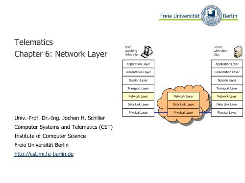
<strong>Telematics</strong><br />
<strong>Chapter</strong> 6: <strong>Network</strong> <strong>Layer</strong><br />
Univ.-Prof. Dr.-Ing. Jochen H. Schiller<br />
Computer Systems and <strong>Telematics</strong> (CST)<br />
Institute of Computer Science<br />
<strong>Freie</strong> <strong>Universität</strong> <strong>Berlin</strong><br />
http://cst.mi.fu-berlin.de<br />
User<br />
watching<br />
video clip<br />
Application <strong>Layer</strong><br />
Presentation <strong>Layer</strong><br />
Session <strong>Layer</strong><br />
Transport <strong>Layer</strong><br />
<strong>Network</strong> <strong>Layer</strong><br />
Data Link <strong>Layer</strong><br />
Physical <strong>Layer</strong><br />
<strong>Network</strong> <strong>Layer</strong><br />
Data Link <strong>Layer</strong><br />
Physical <strong>Layer</strong><br />
Server<br />
with video<br />
clips<br />
Application <strong>Layer</strong><br />
Presentation <strong>Layer</strong><br />
Session <strong>Layer</strong><br />
Transport <strong>Layer</strong><br />
<strong>Network</strong> <strong>Layer</strong><br />
Data Link <strong>Layer</strong><br />
Physical <strong>Layer</strong>
Contents<br />
● Design Issues<br />
● The Internet<br />
● Internet Protocol (IP)<br />
● Internet Protocol Version 6 (IPv6)<br />
● <strong>Network</strong> Address Translation<br />
(NAT)<br />
● Auxiliary Protocols<br />
● Address Resolution Protocols (ARP)<br />
● Reverse ARP (RARP)<br />
● Dynamic Host Configuration<br />
Protocol (DHCP)<br />
● Internet Control Message Protocol<br />
(ICMP)<br />
● Routing<br />
● Shortest Path Routing<br />
● Distance Vector Routing<br />
● Routing Information Protocol (RIP)<br />
● Link State Routing<br />
● Hierarchical Routing<br />
● Open Shortest Path First (OSPF)<br />
● Border Gateway Protocol (BGP)<br />
● Internet Group Management<br />
Protocol (IGMP)<br />
Univ.-Prof. Dr.-Ing. Jochen H. Schiller ▪ cst.mi.fu-berlin.de ▪ <strong>Telematics</strong> ▪ <strong>Chapter</strong> 6: <strong>Network</strong> <strong>Layer</strong><br />
6.2
Design Issues<br />
Connection principles<br />
Univ.-Prof. Dr.-Ing. Jochen H. Schiller ▪ cst.mi.fu-berlin.de ▪ <strong>Telematics</strong> ▪ <strong>Chapter</strong> 6: <strong>Network</strong> <strong>Layer</strong><br />
6.3
<strong>Layer</strong> 3<br />
● <strong>Layer</strong> 1/2 are responsible only for<br />
the transmission of data between<br />
adjacent computers.<br />
● <strong>Layer</strong> 3: <strong>Network</strong> <strong>Layer</strong><br />
● Boundary between network<br />
carrier and customer<br />
● Control of global traffic<br />
● Coupling of sub-networks<br />
● Global addressing<br />
● Routing of data packets<br />
● Initiation, management and<br />
termination of connections through<br />
the whole network<br />
● Global flow control<br />
Univ.-Prof. Dr.-Ing. Jochen H. Schiller ▪ cst.mi.fu-berlin.de ▪ <strong>Telematics</strong> ▪ <strong>Chapter</strong> 6: <strong>Network</strong> <strong>Layer</strong><br />
OSI Reference Model<br />
Application <strong>Layer</strong><br />
Presentation <strong>Layer</strong><br />
Session <strong>Layer</strong><br />
Transport <strong>Layer</strong><br />
<strong>Network</strong> <strong>Layer</strong><br />
Data Link <strong>Layer</strong><br />
Physical <strong>Layer</strong><br />
6.4
<strong>Layer</strong>s in the <strong>Network</strong><br />
Application<br />
Process<br />
Application<br />
<strong>Layer</strong><br />
Presentation<br />
<strong>Layer</strong><br />
Session<br />
<strong>Layer</strong><br />
Transport<br />
<strong>Layer</strong><br />
<strong>Network</strong><br />
<strong>Layer</strong><br />
Data Link<br />
<strong>Layer</strong><br />
Physical<br />
<strong>Layer</strong><br />
Routers in the network receive frames<br />
from layer 2, extract the layer 3 content<br />
(packet) and decide based on the global<br />
address to which outgoing connection<br />
(port) the packet has to be passed on.<br />
Accordingly the packet becomes payload<br />
of a new frame and is sent.<br />
<strong>Network</strong><br />
<strong>Layer</strong><br />
Data Link<br />
<strong>Layer</strong><br />
Physical<br />
<strong>Layer</strong><br />
<strong>Network</strong><br />
<strong>Layer</strong><br />
Data Link<br />
<strong>Layer</strong><br />
Physical<br />
<strong>Layer</strong><br />
Application<br />
Process<br />
Application<br />
<strong>Layer</strong><br />
Presentation<br />
<strong>Layer</strong><br />
Session<br />
<strong>Layer</strong><br />
Transport<br />
<strong>Layer</strong><br />
<strong>Network</strong><br />
<strong>Layer</strong><br />
Data Link<br />
<strong>Layer</strong><br />
Physical<br />
<strong>Layer</strong><br />
Host A Router A Router B<br />
Host B<br />
Univ.-Prof. Dr.-Ing. Jochen H. Schiller ▪ cst.mi.fu-berlin.de ▪ <strong>Telematics</strong> ▪ <strong>Chapter</strong> 6: <strong>Network</strong> <strong>Layer</strong><br />
6.5
<strong>Layer</strong>s in the <strong>Network</strong><br />
<strong>Network</strong> <strong>Layer</strong><br />
Data Link <strong>Layer</strong><br />
Physical <strong>Layer</strong><br />
One protocol on the network layer<br />
Technology 1<br />
Ethernet<br />
MTU 1500 bytes<br />
<strong>Network</strong> <strong>Layer</strong><br />
Data Link <strong>Layer</strong><br />
Physical <strong>Layer</strong><br />
Technology 2<br />
Tokenring, DSL<br />
MTU 512 bytes<br />
Univ.-Prof. Dr.-Ing. Jochen H. Schiller ▪ cst.mi.fu-berlin.de ▪ <strong>Telematics</strong> ▪ <strong>Chapter</strong> 6: <strong>Network</strong> <strong>Layer</strong><br />
<strong>Network</strong> <strong>Layer</strong><br />
Data Link <strong>Layer</strong><br />
Physical <strong>Layer</strong><br />
6.6
Two Fundamental Philosophies<br />
● Connectionless communication (e.g. Internet)<br />
● Data are transferred as packets of variable length<br />
● Source and destination address are being indicated<br />
● Sending is made spontaneously without reservations<br />
● Very easy to implement<br />
● But: packets can take different ways to the receiver<br />
● Wrong order of packets at the receiver, differences in transmission delay, unreliability<br />
● Connection-oriented communication (e.g. telephony)<br />
● Connection establishment:<br />
● Selection of the communication partner resp. of the terminal<br />
● Examination of the communication readiness<br />
● Establishment of a connection<br />
● Data transmission: Information exchange between the partners<br />
● Connection termination: Release of the terminals and channels<br />
● Advantages: no change of sequence, reservation of capacity, flow control<br />
Univ.-Prof. Dr.-Ing. Jochen H. Schiller ▪ cst.mi.fu-berlin.de ▪ <strong>Telematics</strong> ▪ <strong>Chapter</strong> 6: <strong>Network</strong> <strong>Layer</strong><br />
6.7
Connectionless Communication<br />
Computer A<br />
3 2 1<br />
Computer C<br />
Packet Switching<br />
� Message is divided into packets<br />
� Access is always possible, small susceptibility to faults<br />
� Alternative paths for the packets<br />
� Additional effort in the nodes: Store-and-Forward network<br />
Univ.-Prof. Dr.-Ing. Jochen H. Schiller ▪ cst.mi.fu-berlin.de ▪ <strong>Telematics</strong> ▪ <strong>Chapter</strong> 6: <strong>Network</strong> <strong>Layer</strong><br />
Computer B<br />
6.8
Connection-Oriented Communication<br />
Computer A<br />
3<br />
2<br />
Computer C<br />
Circuit Switching<br />
1<br />
� Simple communication method<br />
� Defined routes between the participants<br />
� Switching nodes connect the lines<br />
� Exclusive use of the line (telephone) or virtual connection:<br />
Computer B<br />
virtual connection<br />
� Establishment of a connection over a (possibly even packet switching) network<br />
Univ.-Prof. Dr.-Ing. Jochen H. Schiller ▪ cst.mi.fu-berlin.de ▪ <strong>Telematics</strong> ▪ <strong>Chapter</strong> 6: <strong>Network</strong> <strong>Layer</strong><br />
6.9
Design Issues<br />
Routing principles<br />
Univ.-Prof. Dr.-Ing. Jochen H. Schiller ▪ cst.mi.fu-berlin.de ▪ <strong>Telematics</strong> ▪ <strong>Chapter</strong> 6: <strong>Network</strong> <strong>Layer</strong><br />
6.10
Routing<br />
● Most important functionality on <strong>Layer</strong> 3 is addressing and routing.<br />
● Each computer has to be assigned a worldwide unique address<br />
● Every router manages a table (Routing Table) which indicates, which<br />
outgoing connection has to be selected for a certain destination.<br />
L4<br />
L1<br />
L2<br />
L3<br />
To destination By connection<br />
A L2<br />
B L1<br />
C L3<br />
D L2<br />
● The routing tables can be determined statically; however it is better to<br />
adapt them dynamically to the current network status.<br />
● With connectionless communication, the routing must be done for<br />
each packet separately. The routing decision can vary from packet to<br />
packet.<br />
● With virtual connections, routing is done only once (connection<br />
establishment, see ATM), but the routing tables are more extensive<br />
Univ.-Prof. Dr.-Ing. Jochen H. Schiller ▪ cst.mi.fu-berlin.de ▪ <strong>Telematics</strong> ▪ <strong>Chapter</strong> 6: <strong>Network</strong> <strong>Layer</strong><br />
6.11
Routing<br />
● Task: determine most favorable route from the sender to the receiver<br />
● Short response times<br />
● High throughput<br />
● Avoidance of local overload situations<br />
● Security requirements<br />
● Shortest path<br />
● Routing tables in the nodes can be<br />
● One-dimensional (connectionless): decision depends only on the destination<br />
● Two-dimensional (connection oriented): decision depends on the source and<br />
destination<br />
Sender<br />
A<br />
C<br />
Univ.-Prof. Dr.-Ing. Jochen H. Schiller ▪ cst.mi.fu-berlin.de ▪ <strong>Telematics</strong> ▪ <strong>Chapter</strong> 6: <strong>Network</strong> <strong>Layer</strong><br />
S R<br />
B Receiver<br />
L<br />
6.12
Routing - Connectionless<br />
Univ.-Prof. Dr.-Ing. Jochen H. Schiller ▪ cst.mi.fu-berlin.de ▪ <strong>Telematics</strong> ▪ <strong>Chapter</strong> 6: <strong>Network</strong> <strong>Layer</strong><br />
6.13
Routing - Connection-oriented<br />
Source computer, connection ID Next computer, connection ID<br />
Univ.-Prof. Dr.-Ing. Jochen H. Schiller ▪ cst.mi.fu-berlin.de ▪ <strong>Telematics</strong> ▪ <strong>Chapter</strong> 6: <strong>Network</strong> <strong>Layer</strong><br />
Related terms<br />
� Virtual circuit<br />
� Label switching<br />
6.14
Routing – Comparison<br />
Issue Connectionless<br />
Datagram Subnet<br />
Circuit setup Not needed Required<br />
Addressing Each packet contains the full<br />
source and destination address<br />
State information Routers do not hold state<br />
information about connections<br />
Routing Each packet is routed<br />
independently<br />
Effect of router<br />
failures<br />
None, except for packets lost<br />
during the crash<br />
Connection-oriented<br />
Virtual-circuit Subnet<br />
Each packet contains a short VC ID<br />
Each VC requires router table<br />
space per connection<br />
Route chosen when VC is set up;<br />
all packets follow it<br />
All VCs that passed through the<br />
failed router are terminated<br />
Quality of service Difficult Easy if enough resources can be<br />
allocated in advance for each VC<br />
Congestion control Difficult Easy if enough resources can be<br />
allocated in advance for each VC<br />
Univ.-Prof. Dr.-Ing. Jochen H. Schiller ▪ cst.mi.fu-berlin.de ▪ <strong>Telematics</strong> ▪ <strong>Chapter</strong> 6: <strong>Network</strong> <strong>Layer</strong><br />
6.15
“Optimal” Routing<br />
● “Optimal” route decision is in principle not possible, because<br />
● no complete information about the network is present within the individual nodes<br />
● a routing decision effects the network for a certain period<br />
● conflicts between fairness and optimum can arise<br />
A B C<br />
X X’<br />
A’ B’ C’<br />
Univ.-Prof. Dr.-Ing. Jochen H. Schiller ▪ cst.mi.fu-berlin.de ▪ <strong>Telematics</strong> ▪ <strong>Chapter</strong> 6: <strong>Network</strong> <strong>Layer</strong><br />
● High traffic amount<br />
between A and A’, B<br />
and B’, C and C’<br />
● In order to optimize<br />
the total data flow, no<br />
traffic may occur<br />
between X and X’<br />
● X and X’ would see<br />
this totally different!<br />
fairness criteria!<br />
6.16
The Optimality Principle<br />
A subnet A sink tree for router B<br />
Univ.-Prof. Dr.-Ing. Jochen H. Schiller ▪ cst.mi.fu-berlin.de ▪ <strong>Telematics</strong> ▪ <strong>Chapter</strong> 6: <strong>Network</strong> <strong>Layer</strong><br />
6.17
Delivered packets<br />
Congestion Control<br />
Maximum capacity<br />
of the network<br />
Perfect<br />
Sent packets<br />
Desirable<br />
Overloaded<br />
Solution: “smoothing” of the traffic amount,<br />
i.e., adjustment of the data rate.<br />
With excessive traffic,<br />
the performance of the network<br />
decreases rapidly<br />
Parameters for detecting overload:<br />
● Average length of the router queues<br />
● Portion of the discarded packets in a<br />
router<br />
● Number of packets in a router<br />
● Number of packet retransmissions<br />
● Average transmission delay from the<br />
sender to the receiver<br />
● Standard deviation of the<br />
transmission delay<br />
� Traffic Shaping<br />
Univ.-Prof. Dr.-Ing. Jochen H. Schiller ▪ cst.mi.fu-berlin.de ▪ <strong>Telematics</strong> ▪ <strong>Chapter</strong> 6: <strong>Network</strong> <strong>Layer</strong><br />
6.18
Internet<br />
Univ.-Prof. Dr.-Ing. Jochen H. Schiller ▪ cst.mi.fu-berlin.de ▪ <strong>Telematics</strong> ▪ <strong>Chapter</strong> 6: <strong>Network</strong> <strong>Layer</strong><br />
6.19
On the Way to Today's Internet<br />
● Goal:<br />
● Interconnection of computers and networks using uniform protocols<br />
● A particularly important initiative was initiated by the ARPA<br />
(Advanced Research Project Agency, with military interests)<br />
● The participation of the military was the only sensible way to implement such an<br />
ambitious and extremely expensive project<br />
● The OSI specification was still in developing phase<br />
● Result: ARPANET (predecessor of today's Internet)<br />
Univ.-Prof. Dr.-Ing. Jochen H. Schiller ▪ cst.mi.fu-berlin.de ▪ <strong>Telematics</strong> ▪ <strong>Chapter</strong> 6: <strong>Network</strong> <strong>Layer</strong><br />
6.20
On the Way to Today's Internet<br />
Structure of the<br />
telephone system.<br />
Baran’s proposed distributed<br />
switching system.<br />
Univ.-Prof. Dr.-Ing. Jochen H. Schiller ▪ cst.mi.fu-berlin.de ▪ <strong>Telematics</strong> ▪ <strong>Chapter</strong> 6: <strong>Network</strong> <strong>Layer</strong><br />
6.21
ARPANET<br />
Design objective for ARPANET<br />
● The operability of the network should remain<br />
intact even after a large disaster, e.g., a nuclear<br />
war, thus high connectivity and<br />
connectionless transmission<br />
● <strong>Network</strong> computers and host computers are<br />
separated<br />
Subnet<br />
Univ.-Prof. Dr.-Ing. Jochen H. Schiller ▪ cst.mi.fu-berlin.de ▪ <strong>Telematics</strong> ▪ <strong>Chapter</strong> 6: <strong>Network</strong> <strong>Layer</strong><br />
ARPA<br />
Advanced Research<br />
Projects Agency<br />
ARPANET<br />
1969<br />
6.22
ARPANET<br />
A node consists of<br />
● an IMP<br />
● a host<br />
A subnet consists of:<br />
● Interface Message Processors<br />
(IMPs), which are connected by<br />
leased transmission circuits<br />
● High connectivity (in order to<br />
guarantee the demanded<br />
reliability)<br />
Several protocols for the<br />
communication between<br />
IMP-IMP, host-IMP,…<br />
Host-IMP<br />
Protocol<br />
Host-host Protocol<br />
Source IMP to<br />
destination IMP protocol<br />
Subnet<br />
Univ.-Prof. Dr.-Ing. Jochen H. Schiller ▪ cst.mi.fu-berlin.de ▪ <strong>Telematics</strong> ▪ <strong>Chapter</strong> 6: <strong>Network</strong> <strong>Layer</strong><br />
IMP<br />
6.23
The Beginning of ARPANET<br />
IBM<br />
360/75<br />
University of<br />
California Santa<br />
Barbara (UCSB)<br />
IMP<br />
XDS<br />
940<br />
IMP<br />
XDS<br />
1-7<br />
Stanford Research<br />
Institute (SRI)<br />
IMP<br />
IMP California<br />
University of California<br />
Los Angeles (UCLA)<br />
DEK<br />
PDP-<br />
10<br />
University<br />
of Utah<br />
Univ.-Prof. Dr.-Ing. Jochen H. Schiller ▪ cst.mi.fu-berlin.de ▪ <strong>Telematics</strong> ▪ <strong>Chapter</strong> 6: <strong>Network</strong> <strong>Layer</strong><br />
ARPANET<br />
(December 1969)<br />
6.24
Evolution by ARPANET<br />
Very fast evolution of the ARPANET within shortest time:<br />
UCSB<br />
SRI<br />
UCLA<br />
Utah<br />
USC<br />
Illinois<br />
WITH<br />
Harvard<br />
UCSB<br />
UCLA<br />
SRI Utah Illinois WITH<br />
Stanford<br />
USC<br />
Harvard<br />
Aberdeen<br />
CMU<br />
ARPANET in April 1972 ARPANET in September 1972<br />
Univ.-Prof. Dr.-Ing. Jochen H. Schiller ▪ cst.mi.fu-berlin.de ▪ <strong>Telematics</strong> ▪ <strong>Chapter</strong> 6: <strong>Network</strong> <strong>Layer</strong><br />
6.25
Interworking<br />
● Problem: Interworking!<br />
● Simultaneously to the ARPANET other (smaller) networks were developed<br />
● All the LANs, MANs, WANs, ...<br />
● had different protocols, media, ...<br />
● could not be interconnected at first and were not be able to communicate with<br />
each other<br />
● Therefore:<br />
● Development of uniform protocols on the transport- and network level<br />
● without a too accurate definition of these levels, in particular without exact coordination<br />
with the respective OSI levels<br />
● Result: TCP/IP networks<br />
Univ.-Prof. Dr.-Ing. Jochen H. Schiller ▪ cst.mi.fu-berlin.de ▪ <strong>Telematics</strong> ▪ <strong>Chapter</strong> 6: <strong>Network</strong> <strong>Layer</strong><br />
6.26
TCP/IP<br />
● Developed 1974:<br />
● Transmission Control Protocol/Internet Protocol (TCP/IP)<br />
● Requirements:<br />
● Fault tolerance<br />
● Maximum possible reliability and availability<br />
● Flexibility, i.e., suitability for applications with very different requirements<br />
● The result:<br />
● <strong>Network</strong> protocol<br />
● Internet Protocol (IP), connectionless<br />
● End-to-end protocols<br />
● Transmission Control Protocol (TCP), connection-oriented<br />
● User Datagram Protocol (UDP), connectionless<br />
Univ.-Prof. Dr.-Ing. Jochen H. Schiller ▪ cst.mi.fu-berlin.de ▪ <strong>Telematics</strong> ▪ <strong>Chapter</strong> 6: <strong>Network</strong> <strong>Layer</strong><br />
6.27
TCP/IP and the OSI Reference Model<br />
Application <strong>Layer</strong><br />
Presentation <strong>Layer</strong><br />
Session <strong>Layer</strong><br />
Transport <strong>Layer</strong><br />
<strong>Network</strong> <strong>Layer</strong><br />
Data Link <strong>Layer</strong><br />
Physical <strong>Layer</strong><br />
Application <strong>Layer</strong><br />
Do not exist!<br />
Transport <strong>Layer</strong> (TCP/UDP)<br />
Internet <strong>Layer</strong> (IP)<br />
Host-to-<strong>Network</strong> <strong>Layer</strong><br />
ISO/OSI TCP/IP<br />
Univ.-Prof. Dr.-Ing. Jochen H. Schiller ▪ cst.mi.fu-berlin.de ▪ <strong>Telematics</strong> ▪ <strong>Chapter</strong> 6: <strong>Network</strong> <strong>Layer</strong><br />
6.28
From the ARPANET to the Internet<br />
● 1983 TCP/IP became the official protocol of ARPANET<br />
● ARPANET was connected with many other USA networks<br />
● Intercontinental connecting with networks in Europe, Asia, Pacific<br />
● The total network evolved this way to a world-wide available network<br />
(called “Internet”) and gradually lost its early militarily dominated<br />
character<br />
● No central administrated network, but a world-wide union from many<br />
individual, different networks under local control (and financing)<br />
● 1990 the Internet consisted of 3,000 networks with 200,000 computers.<br />
That was however only the beginning of a rapid evolution<br />
Univ.-Prof. Dr.-Ing. Jochen H. Schiller ▪ cst.mi.fu-berlin.de ▪ <strong>Telematics</strong> ▪ <strong>Chapter</strong> 6: <strong>Network</strong> <strong>Layer</strong><br />
6.29
Evolution of the Internet<br />
● Until 1990: the Internet was comparatively small, only used by universities<br />
and research institutions<br />
● 1990: The WWW (World Wide Web) became the “killer application”<br />
� breakthrough for the acceptance of the Internet<br />
● developed by CERN for the simplification of communication in the field of highenergy<br />
physics<br />
● HTML as markup language and Netscape as web browser<br />
● Emergence of so-called Internet Service Providers (ISP)<br />
● Companies that provide access points to the Internet<br />
● Millions of new users, predominantly non-academic!<br />
● New applications, e.g., E-Commerce, E-Learning, E-Governance, …<br />
● 1995: Backbones, ten thousands LANs, millions attached computers,<br />
exponentially rising number of users<br />
● 1998: The number of attached computers is doubled approx. every 6<br />
months<br />
● 1999: The transferred data volume is doubled in less than 4 months<br />
Univ.-Prof. Dr.-Ing. Jochen H. Schiller ▪ cst.mi.fu-berlin.de ▪ <strong>Telematics</strong> ▪ <strong>Chapter</strong> 6: <strong>Network</strong> <strong>Layer</strong><br />
6.30
Evolution of the Internet<br />
Univ.-Prof. Dr.-Ing. Jochen H. Schiller ▪ cst.mi.fu-berlin.de ▪ <strong>Telematics</strong> ▪ <strong>Chapter</strong> 6: <strong>Network</strong> <strong>Layer</strong><br />
6.31
Evolution in Germany<br />
Univ.-Prof. Dr.-Ing. Jochen H. Schiller ▪ cst.mi.fu-berlin.de ▪ <strong>Telematics</strong> ▪ <strong>Chapter</strong> 6: <strong>Network</strong> <strong>Layer</strong><br />
http://www.denic.de/hintergrund/statistiken.html<br />
6.32
Internet<br />
● What does it mean: “a computer is connected to the Internet”?<br />
● Use of the TCP/IP protocol suite<br />
● Accessibility over a global IP address<br />
● Ability to send IP packets<br />
● In its early period, the Internet was limited to the following applications:<br />
● Remote login<br />
● Running jobs on external computers<br />
● File transfer<br />
● Exchange of data between computers<br />
● E-mail<br />
● Electronic mail<br />
Univ.-Prof. Dr.-Ing. Jochen H. Schiller ▪ cst.mi.fu-berlin.de ▪ <strong>Telematics</strong> ▪ <strong>Chapter</strong> 6: <strong>Network</strong> <strong>Layer</strong><br />
6.33
Internet vs. Intranet<br />
● Internet<br />
● Communication via the TCP/IP<br />
protocols<br />
● Local operators control and finance<br />
● Global coordination by some<br />
organizations<br />
● Internet Service Providers (ISP)<br />
provide access points for private<br />
individuals<br />
● Intranet<br />
Univ.-Prof. Dr.-Ing. Jochen H. Schiller ▪ cst.mi.fu-berlin.de ▪ <strong>Telematics</strong> ▪ <strong>Chapter</strong> 6: <strong>Network</strong> <strong>Layer</strong><br />
● Enterprise-internal communication<br />
with the same protocols and<br />
applications as in the Internet<br />
● Computers are sealed off from the<br />
global Internet (security)<br />
● Heterogeneous network structures<br />
from different branches can be<br />
integrated with TCP/IP easily<br />
● Use of applications like in the WWW<br />
for internal data exchange<br />
6.34
The classical TCP/IP Protocol Suite<br />
Protocols<br />
<strong>Network</strong>s<br />
HTTP<br />
IGMP<br />
FTP Telnet SMTP DNS SNMP TFTP<br />
TCP<br />
Ethernet Token Ring Token Bus<br />
UDP<br />
ICMP IP ARP RARP<br />
Univ.-Prof. Dr.-Ing. Jochen H. Schiller ▪ cst.mi.fu-berlin.de ▪ <strong>Telematics</strong> ▪ <strong>Chapter</strong> 6: <strong>Network</strong> <strong>Layer</strong><br />
Wireless LAN<br />
Application<br />
<strong>Layer</strong><br />
Transport<br />
<strong>Layer</strong><br />
Internet<br />
<strong>Layer</strong><br />
Host-tonetwork<br />
<strong>Layer</strong><br />
6.35
Classical Sandglass Model<br />
● Sandglass model<br />
● Small number of central protocols<br />
● Large number of applications and<br />
communication networks<br />
E-Mail, File Transfer,<br />
Video Conferencing, …<br />
Univ.-Prof. Dr.-Ing. Jochen H. Schiller ▪ cst.mi.fu-berlin.de ▪ <strong>Telematics</strong> ▪ <strong>Chapter</strong> 6: <strong>Network</strong> <strong>Layer</strong><br />
HTTP, SMTP, FTP, …<br />
Twisted Pair, Optical Fiber,<br />
Radio, …<br />
6.36
Internet Protocol (IP)<br />
Univ.-Prof. Dr.-Ing. Jochen H. Schiller ▪ cst.mi.fu-berlin.de ▪ <strong>Telematics</strong> ▪ <strong>Chapter</strong> 6: <strong>Network</strong> <strong>Layer</strong><br />
6.37
Internet <strong>Layer</strong><br />
● Raw division into three tasks:<br />
● Data transfer over a global network<br />
● Route decision at the sub-nodes<br />
● Control of the network or transmission status<br />
Routing Protocols<br />
Routing Tables<br />
Transfer Protocols<br />
IPv4, IPv6<br />
“Control” Protocols<br />
ICMP, ARP, RARP, IGMP<br />
Univ.-Prof. Dr.-Ing. Jochen H. Schiller ▪ cst.mi.fu-berlin.de ▪ <strong>Telematics</strong> ▪ <strong>Chapter</strong> 6: <strong>Network</strong> <strong>Layer</strong><br />
6.38
Internet Protocol (IP)<br />
● IP: connectionless, unreliable transmission of datagrams/packets<br />
�“Best Effort” Service<br />
● Transparent end-to-end communication between the hosts<br />
● Routing, interoperability between different network types<br />
● IP addressing (IPv4)<br />
● Uses logical 32-bit addresses<br />
● Hierarchical addressing<br />
● 3 network classes<br />
● 4 address formats (including multicast)<br />
● Fragmenting and reassembling of packets<br />
● Maximum packet size: 64 kByte<br />
● In practice: 1500 byte<br />
● At present commonly used: Version 4 of IP (IPv4)<br />
Univ.-Prof. Dr.-Ing. Jochen H. Schiller ▪ cst.mi.fu-berlin.de ▪ <strong>Telematics</strong> ▪ <strong>Chapter</strong> 6: <strong>Network</strong> <strong>Layer</strong><br />
6.39
IP Packet<br />
Version<br />
IHL<br />
32 Bits (4 Bytes)<br />
Type of<br />
Service<br />
Source Address<br />
Total Length<br />
D M<br />
Identification Fragment Offset<br />
F F<br />
Time to Live Protocol Header Checksum<br />
Destination Address<br />
Options (variable, 0-40 Byte)<br />
Data (variable)<br />
Padding<br />
Univ.-Prof. Dr.-Ing. Jochen H. Schiller ▪ cst.mi.fu-berlin.de ▪ <strong>Telematics</strong> ▪ <strong>Chapter</strong> 6: <strong>Network</strong> <strong>Layer</strong><br />
IP Header,<br />
usually 20 Bytes<br />
Header Data<br />
6.40
The IP Header (1)<br />
● Version (4 bits): IP version number (for simultaneous use of several IP versions)<br />
● IHL (4 bits): IP Header Length (in words of 32 bit; between 5 and 15, depending<br />
upon options)<br />
● Type of Service (8 bits): Indication of the desired service: Combination of reliability<br />
(e.g. file transfer) and speed (e.g. audio) � historical, DSCP today<br />
3 bit priority<br />
(0 = normal data,<br />
7 = control packet)<br />
● Total Length (16 bits): Length of the entire packet � 2 16 -1 = 65,535 bytes<br />
● Identification (16 bits): definite marking of a packet<br />
● Time to Live (TTL, 8 bits):<br />
Precedence D T R unused<br />
Delay Throughput<br />
Version<br />
Reliability<br />
IHL<br />
Type of<br />
Service<br />
Total Length<br />
Identification<br />
D M<br />
F F<br />
Fragment Offset<br />
Time to Live Protocol Header Checksum<br />
● To prevent the endless circling of packets in the network the lifetime of packets is limited to a<br />
Source Address<br />
maximum of 255 hops.<br />
Destination Address<br />
● In principle, the processing time in routers has to be considered, which does not happen in<br />
practice. The counter is reduced with each hop, with 0 the packet Options (variable, is discarded. 0-40 Byte)<br />
Univ.-Prof. Dr.-Ing. Jochen H. Schiller ▪ cst.mi.fu-berlin.de ▪ <strong>Telematics</strong> ▪ <strong>Chapter</strong> 6: <strong>Network</strong> <strong>Layer</strong><br />
DATA (variable)<br />
Padding<br />
6.41
The IP Header (2)<br />
● DF (1 bit): Don't Fragment. All routers must forward packets up to a size of 576<br />
byte, everything beyond that is optional. Larger packets with set DF-bit therefore<br />
cannot take each possible way in the network.<br />
● MF (1 bit): More Fragments<br />
● “1” - further fragments follow<br />
● “0” - last fragment of a datagram<br />
● Fragment Offset (13 bits): Sequence number of the fragments of a packet (2 13<br />
= 8192 possible fragments). The offset states, to which position of a packet<br />
(counted in multiples of 8 byte) a fragment belongs to. From this a maximum<br />
length of 8192 x 8 byte = 65,536 byte results for a packet.<br />
● Protocol (8 bits): Which transport protocol is used in the data part (UDP,<br />
Type of<br />
TCP,…)? To which transport process the packet has Version to IHL be passed? Service<br />
Total Length<br />
D M<br />
Identification Fragment Offset<br />
● Header Checksum (16 bits): 1’s complement of the sum of the 16-bit F F half<br />
words of the header. Must be computed with each hop (since Protocol TTL changes)<br />
Time to Live Header Checksum<br />
Source Address<br />
● Source Address/Destination Address (32 bits): <strong>Network</strong> and host numbers<br />
Destination Address<br />
of sending and receiving computer. This information is used by routers for the<br />
routing decision.<br />
Options (variable, 0-40 Byte)<br />
Univ.-Prof. Dr.-Ing. Jochen H. Schiller ▪ cst.mi.fu-berlin.de ▪ <strong>Telematics</strong> ▪ <strong>Chapter</strong> 6: <strong>Network</strong> <strong>Layer</strong><br />
DATA (variable)<br />
Padding<br />
6.42
Fragmentation<br />
● A too large or too small packet length prevents a good performance. Additionally<br />
there are often size restrictions (buffer, protocols with length specifications,<br />
standards, allowed access time to a channel,…)<br />
● The data length must be a multiple of 8 byte. Exception: the last fragment, only<br />
the remaining data are packed, padding to 8 byte units is not applied.<br />
● If the “DF”-bit is set, the fragmentation is prevented.<br />
ID Flags Offset Data<br />
777 x00 0 0 1200 bytes<br />
IP header<br />
777 x01 0 0 511<br />
777 x01 64 512 1023<br />
Univ.-Prof. Dr.-Ing. Jochen H. Schiller ▪ cst.mi.fu-berlin.de ▪ <strong>Telematics</strong> ▪ <strong>Chapter</strong> 6: <strong>Network</strong> <strong>Layer</strong><br />
777 x00 128 1024 1200<br />
6.43
The IP Header (3)<br />
● Options (≤40 bytes): Prepare for future protocol extensions.<br />
● Coverage: Multiple of 4 byte, therefore possibly padding is necessary<br />
● See for details: www.iana.org/assignments/ip-parameters<br />
● Five options are defined, however none is supported by common routers:<br />
● Security: How secret is the transported information?<br />
● Application e.g. in military: Avoidance of crossing of certain countries/networks.<br />
● Strict Source Routing: Complete path defined from the source to the<br />
destination host by providing the IP addresses of all routers which are crossed.<br />
● For managers e.g. in case of damaged routing tables or for time measurements<br />
● Loose Source Routing: The carried list of routers must be passed in indicated<br />
order. Additional routers are permitted.<br />
● Record Route: Recording of the IP addresses of the routers passed.<br />
● Maximally 9 IP addresses possible, nowadays too few.<br />
● Time Stamp: Records router addresses (32 bits) as well as a time stamp for<br />
each router (32 bits). Application e.g. in fault management.<br />
Univ.-Prof. Dr.-Ing. Jochen H. Schiller ▪ cst.mi.fu-berlin.de ▪ <strong>Telematics</strong> ▪ <strong>Chapter</strong> 6: <strong>Network</strong> <strong>Layer</strong><br />
6.44
Internet Protocol (IP)<br />
Addressing<br />
Univ.-Prof. Dr.-Ing. Jochen H. Schiller ▪ cst.mi.fu-berlin.de ▪ <strong>Telematics</strong> ▪ <strong>Chapter</strong> 6: <strong>Network</strong> <strong>Layer</strong><br />
6.45
Classical IP Addressing<br />
● Unique IP address for each host and router.<br />
● IP addresses are 32 bits long and are used in the Source Address as well as in the<br />
Destination Address field of IP packets.<br />
● The IP address is structured hierarchically and refers to a certain network, i.e.,<br />
machines with connection to several networks have several IP addresses.<br />
● Structure of the address: <strong>Network</strong> address for physical network (e.g. 160.45.117.0) and<br />
host address for a machine in the addressed network (e.g. 160.45.117.199)<br />
Class<br />
A<br />
B<br />
C<br />
D<br />
E<br />
32 bits<br />
0 <strong>Network</strong> Host<br />
10 <strong>Network</strong> Host<br />
110 <strong>Network</strong> Host<br />
1110 Multicast address<br />
1111 Reserved for future use<br />
Univ.-Prof. Dr.-Ing. Jochen H. Schiller ▪ cst.mi.fu-berlin.de ▪ <strong>Telematics</strong> ▪ <strong>Chapter</strong> 6: <strong>Network</strong> <strong>Layer</strong><br />
126 networks with<br />
2 24 hosts each<br />
(starting from 1.0.0.0)<br />
16,383 networks with<br />
2 16 hosts each<br />
(starting from 128.0.0.0)<br />
2,097,151 networks<br />
(LANs) with<br />
256 hosts each<br />
(starting from 192.0.0.0)<br />
6.46
IP Addresses<br />
192.168.13.x<br />
192.168.13.21<br />
192.168.13.0<br />
Binary format<br />
Dotted Decimal Notation<br />
192.168.13.1<br />
147.216.113.1<br />
147.216.113.y<br />
11000000 . 10101000 . 00001101 . 00010101<br />
192.168.13.21<br />
● Each node has (at least) one world-wide unique IP address<br />
147.216.113.0<br />
147.216.113.71<br />
● Router or gateways that link several networks, have for each network an IP address<br />
Univ.-Prof. Dr.-Ing. Jochen H. Schiller ▪ cst.mi.fu-berlin.de ▪ <strong>Telematics</strong> ▪ <strong>Chapter</strong> 6: <strong>Network</strong> <strong>Layer</strong><br />
6.47
IP Addresses and Routing<br />
Server Server<br />
Server<br />
Computer<br />
Server<br />
Ethernet<br />
Computer<br />
Ethernet<br />
Computer<br />
Server<br />
142.117.0.0<br />
147.216.0.0<br />
Computer<br />
Computer Server<br />
Ethernet<br />
Computer<br />
a<br />
Destination<br />
IP Address<br />
Computer<br />
b<br />
Computer<br />
Server<br />
Ethernet<br />
Connection <strong>Network</strong><br />
Interface<br />
12.x.x.x 194.52.124.x b<br />
147.216.x.x 142.117.x.x a<br />
142.117.x.x direct a<br />
194.52.124.x direct b<br />
x.x.x.x default a<br />
Server<br />
12.0.0.0<br />
Univ.-Prof. Dr.-Ing. Jochen H. Schiller ▪ cst.mi.fu-berlin.de ▪ <strong>Telematics</strong> ▪ <strong>Chapter</strong> 6: <strong>Network</strong> <strong>Layer</strong><br />
Computer<br />
Computer<br />
Server<br />
Ethernet<br />
Server<br />
Ethernet<br />
Server<br />
Computer<br />
194.52.124.0<br />
Computer<br />
Computer<br />
6.48
IP Addressing: Examples<br />
The representation of the 32-bit addresses is divided into 4 sections of each 8 bits:<br />
www.fu-berlin.de = 160.45.170.10<br />
Class B address<br />
10100000 00101101 10101010 00001010<br />
Special addresses:<br />
Class B address<br />
of FU <strong>Berlin</strong><br />
0 0 0 .............................................................. 0 0 0 This host<br />
Subnet Terminal<br />
0 0 ................. 0 0 Host Host in this network<br />
1 1 1 .............................................................. 1 1 1 Broadcast in own local area network<br />
<strong>Network</strong> 1 1 1 ................................. 1 1 1 Broadcast in the remote network<br />
127 arbitrary Local loop, no sending to the network<br />
Univ.-Prof. Dr.-Ing. Jochen H. Schiller ▪ cst.mi.fu-berlin.de ▪ <strong>Telematics</strong> ▪ <strong>Chapter</strong> 6: <strong>Network</strong> <strong>Layer</strong><br />
6.49
Address Space<br />
14%<br />
6%<br />
25%<br />
Address Space<br />
6%<br />
50%<br />
Univ.-Prof. Dr.-Ing. Jochen H. Schiller ▪ cst.mi.fu-berlin.de ▪ <strong>Telematics</strong> ▪ <strong>Chapter</strong> 6: <strong>Network</strong> <strong>Layer</strong><br />
Class A<br />
Class B<br />
Class C<br />
Class D<br />
Class E<br />
6.50
IP Addresses are scarce…<br />
● Problems<br />
● Nobody had thought about the explosive growth of the Internet<br />
(otherwise one would have defined longer addresses from the beginning).<br />
● Too many Class A address blocks were assigned in the first Internet years.<br />
● Inefficient use of the address space.<br />
● Example: if 500 devices in an enterprise are to be attached, a Class B address<br />
block is needed, but by this unnecessarily more than 65,000 host addresses are<br />
blocked.<br />
● Solution approach: Extension of the address space in IPv6<br />
IP version 6 has 128 bits for addresses � 2 128 addresses<br />
7 x 10²³ IP addresses per square meter of the earth's surface (including the<br />
oceans!)<br />
one address per molecule on earth's surface!<br />
● But: The success of IPv6 is not by any means safe!<br />
● The introduction of IPv6 is tremendously difficult: Interoperability, costs,<br />
migration strategies, …<br />
Univ.-Prof. Dr.-Ing. Jochen H. Schiller ▪ cst.mi.fu-berlin.de ▪ <strong>Telematics</strong> ▪ <strong>Chapter</strong> 6: <strong>Network</strong> <strong>Layer</strong><br />
6.51
IP Subnets<br />
● Problem: Class C-networks (256 hosts) are very small and Class Bnetworks<br />
(65536 hosts) often too large<br />
● Therefore, divide a network into subnets<br />
Rest<br />
of the<br />
Internet<br />
Example for subnets: subnet mask 255.255.255.0<br />
All traffic<br />
for 128.10.0.0<br />
Ethernet A 128.10.1.0<br />
128.10.1.3 128.10.1.8 128.10.1.70 128.10.1.26<br />
128.10.2.1<br />
Private <strong>Network</strong><br />
Ethernet B 128.10.2.0<br />
128.10.1.0<br />
128.10.2.0<br />
128.10.3.0<br />
128.10.4.0<br />
…<br />
128.10.2.3 128.10.2.133 128.10.2.18<br />
Univ.-Prof. Dr.-Ing. Jochen H. Schiller ▪ cst.mi.fu-berlin.de ▪ <strong>Telematics</strong> ▪ <strong>Chapter</strong> 6: <strong>Network</strong> <strong>Layer</strong><br />
6.52
IP Subnets<br />
● Within an IP network address block, several physical networks can be<br />
addressed<br />
● Some bits of the host address part are used as network ID<br />
● A Subnet Mask identifies the “abused” bits<br />
Class B address<br />
Subnet Mask<br />
<strong>Network</strong><br />
1 1 1 1 1 1 1 1 1 1 1 1 1 1 1 1 1 1 1 1 1 1 0 0 0 0 0 0 0 0 0 0<br />
10 <strong>Network</strong> Subnet<br />
Host<br />
● All hosts of a network use the same subnet mask<br />
● Routers can determine through combination of an IP address and a subnet<br />
mask, to which subnet a packet must be sent<br />
Univ.-Prof. Dr.-Ing. Jochen H. Schiller ▪ cst.mi.fu-berlin.de ▪ <strong>Telematics</strong> ▪ <strong>Chapter</strong> 6: <strong>Network</strong> <strong>Layer</strong><br />
6.53
IP Subnets: Computation of the Destination<br />
The entrance router of the FU <strong>Berlin</strong>, which receives the IP packet, does not know,<br />
where host “117.200” is located.<br />
160 45 117 200<br />
IP address<br />
Subnet mask<br />
<strong>Network</strong> of the addressed host<br />
0111 1000<br />
10100000<br />
00101101 01110101 11001000<br />
255 255 0 0<br />
1111 1111<br />
1111 1111<br />
0000 0000<br />
0000 0000<br />
160 45 0 0<br />
10100000<br />
00101101<br />
AND<br />
00000000<br />
00000000<br />
A router computes the subnet “160.45.0.0” and sends the packet to the router,<br />
which links this subnet.<br />
Univ.-Prof. Dr.-Ing. Jochen H. Schiller ▪ cst.mi.fu-berlin.de ▪ <strong>Telematics</strong> ▪ <strong>Chapter</strong> 6: <strong>Network</strong> <strong>Layer</strong><br />
6.54
IP Subnets: Computation of the Destination<br />
The entrance router of the FU <strong>Berlin</strong>, which receives the IP packet, does not know,<br />
where host “117.200” is located.<br />
160 45 117 200<br />
IP address<br />
Subnet mask<br />
<strong>Network</strong> of the addressed host<br />
0111 1000<br />
10100000<br />
00101101 01110101 11001000<br />
255 255 224 0<br />
1111 1111<br />
1111 1111<br />
1110 0000<br />
0000 0000<br />
160 45 96 0<br />
10100000<br />
00101101<br />
AND<br />
01100000<br />
00000000<br />
A router computes the subnet “160.45.96.0” and sends the packet to the router,<br />
which links this subnet.<br />
Univ.-Prof. Dr.-Ing. Jochen H. Schiller ▪ cst.mi.fu-berlin.de ▪ <strong>Telematics</strong> ▪ <strong>Chapter</strong> 6: <strong>Network</strong> <strong>Layer</strong><br />
6.55
Classless Inter-Domain Routing (CIDR)<br />
● Problem:<br />
● Static categorization of IP addresses - how to use the very small class C<br />
networks efficiently?<br />
● Remedy: Classless Inter-Domain Routing (CIDR)<br />
● Weakening of the rigid categorization by replacing the static classes by network<br />
prefixes of variable length<br />
● Form of an IP address: a.b.c.d/n<br />
● The first n bits are the network identification<br />
● The remaining (32 – n) bits are the host identification<br />
● Example: 147.250.3/17<br />
● The first 17 bits are network ID<br />
and<br />
the remaining 15 bits are host ID<br />
10010011.11111010.00000011.00000000<br />
<strong>Network</strong> ID Host ID<br />
● Used together with routing: Backbone router, e.g., on transatlantic links only<br />
considers the first n bits; thus small routing tables, little cost of routing decision<br />
Univ.-Prof. Dr.-Ing. Jochen H. Schiller ▪ cst.mi.fu-berlin.de ▪ <strong>Telematics</strong> ▪ <strong>Chapter</strong> 6: <strong>Network</strong> <strong>Layer</strong><br />
6.56
IPv6<br />
Univ.-Prof. Dr.-Ing. Jochen H. Schiller ▪ cst.mi.fu-berlin.de ▪ <strong>Telematics</strong> ▪ <strong>Chapter</strong> 6: <strong>Network</strong> <strong>Layer</strong><br />
6.57
The new IP: IPv6<br />
IPv6 (December 1998, RFC 2460)<br />
IPv6 (December 1995, RFC 1883)<br />
Publication of the standard (January 1995, RFC 1752)<br />
Specification for IPng (December 1994, RFC 1726)<br />
First requirements for IPng (December 1993, RFC 1550)<br />
Simpler structure of the headers<br />
More automatism<br />
Simpler configuration<br />
Performance improvements<br />
Migration strategies<br />
More security<br />
Larger address space<br />
IPv4 (September 1981, RFC 791)<br />
Univ.-Prof. Dr.-Ing. Jochen H. Schiller ▪ cst.mi.fu-berlin.de ▪ <strong>Telematics</strong> ▪ <strong>Chapter</strong> 6: <strong>Network</strong> <strong>Layer</strong><br />
ST-II (RFC1190)<br />
ST2+ (RFC 1819)<br />
“IPv5”<br />
Stream oriented,<br />
never accepted,<br />
concepts in MPLS,<br />
originally for voice<br />
6.58
IPv6<br />
● Why changing the protocol, when IPv4 works well?<br />
● Dramatically increasing need for new IP addresses<br />
● Improved support of real time applications<br />
● Security mechanisms (Authentication and data protection)<br />
● Differentiation of types of service, in particular for real time applications<br />
● Support of mobility (hosts can go on journeys without address change)<br />
● Simplification of the protocol in order to ensure a faster processing<br />
● Reduction of the extent of the routing tables<br />
● Option for further development of the protocol<br />
Univ.-Prof. Dr.-Ing. Jochen H. Schiller ▪ cst.mi.fu-berlin.de ▪ <strong>Telematics</strong> ▪ <strong>Chapter</strong> 6: <strong>Network</strong> <strong>Layer</strong><br />
6.59
Changes from IPv4 to IPv6<br />
● Changes fall into following categories (RFC 1883, RFC 2460)<br />
● Expanded Addressing Capabilities<br />
● Header Format Simplification<br />
● Improved Support for Extensions and Options<br />
● Flow Labeling Capability � Integrated Services<br />
● Authentication and Privacy Capabilities<br />
Univ.-Prof. Dr.-Ing. Jochen H. Schiller ▪ cst.mi.fu-berlin.de ▪ <strong>Telematics</strong> ▪ <strong>Chapter</strong> 6: <strong>Network</strong> <strong>Layer</strong><br />
6.60
IPv6: Characteristics<br />
● Address size<br />
● 128-bit addresses (8 groups of each 4 hexadecimal numbers)<br />
● Improved option mechanism<br />
● Simplifies and accelerates the processing of IPv6 packets in routers<br />
● Auto-configuration of addresses<br />
● Dynamic allocation of IPv6-addresses<br />
● Improvement of the address flexibility<br />
● Anycast address: Reach any one out of several<br />
● Support of the reservation of resources<br />
● Marking of packets for special traffic<br />
● Security mechanisms<br />
● Authentication and Privacy<br />
● Simpler header structure:<br />
● IHL: redundant, no variable length of header by new option mechanism<br />
● Protocol, fragmentation fields: redundant, moved into the options<br />
● Checksum: Already done by layer 2 and 4<br />
Univ.-Prof. Dr.-Ing. Jochen H. Schiller ▪ cst.mi.fu-berlin.de ▪ <strong>Telematics</strong> ▪ <strong>Chapter</strong> 6: <strong>Network</strong> <strong>Layer</strong><br />
6.61
IPv6 Header<br />
● Version: IP version number (4 bits)<br />
● Traffic Class: classifying packets (8 bits)<br />
● Flow label: virtual connection with certain<br />
characteristics/requirements (20 bits)<br />
● PayloadLen: packet length after the 40byte<br />
header (16 bits)<br />
● Next Header: Indicates the type of the<br />
following extension header or the transport<br />
header (8 bits)<br />
● HopLimit: At each node decremented by<br />
one. At zero the packet is discarded (8 bits)<br />
● Source Address: The address of the<br />
original sender of the packet (128 bits)<br />
● Destination Address: The address of the<br />
receiver (128 bits).<br />
● Not necessarily the final destination, if<br />
there is an optional routing header<br />
● Next Header/Data: if an extension<br />
header is specified, it follows after the main<br />
header. Otherwise, the data are following<br />
1 4 8 16 24<br />
32<br />
Version<br />
(4)<br />
Traffic<br />
Class (8)<br />
PayloadLen (16)<br />
Univ.-Prof. Dr.-Ing. Jochen H. Schiller ▪ cst.mi.fu-berlin.de ▪ <strong>Telematics</strong> ▪ <strong>Chapter</strong> 6: <strong>Network</strong> <strong>Layer</strong><br />
Source Address (128)<br />
Next Header/Data<br />
Flow label (20)<br />
Destination Address (128)<br />
Next Header (8) HopLimit (8)<br />
The prefix of an address characterizes<br />
geographical areas, providers, local internal<br />
areas,…<br />
6.62
IPv6 Header<br />
● Packet size requirements<br />
● IPv6 requires that every link has MTU ≥ 1280 bytes<br />
● Links which cannot convey 1280 byte packets has to apply link-specific<br />
fragmentation and assembly at a layer below IPv6<br />
● Links that have a configurable MTU must be configured to have an MTU of at<br />
least 1280 bytes<br />
● It is recommended that they be configured with an MTU ≥ 1500 bytes<br />
Univ.-Prof. Dr.-Ing. Jochen H. Schiller ▪ cst.mi.fu-berlin.de ▪ <strong>Telematics</strong> ▪ <strong>Chapter</strong> 6: <strong>Network</strong> <strong>Layer</strong><br />
6.63
IPv4 vs. IPv6: Header<br />
Ver- En<br />
sion<br />
4 8 16 32<br />
Type OF of<br />
IHL Totally Total Length length<br />
Service service<br />
Identification<br />
Fragment offset<br />
Time to<br />
Live<br />
Protocol Header Checksum<br />
SOURCE Source ADDRESS Address<br />
Destination ADDRESS Address<br />
Options Option (variable)/Padding<br />
DATA Data<br />
The IPv6 header is longer, but this is only<br />
caused by the longer addresses. Otherwise<br />
it is “better sorted” and thus faster to<br />
process by routers.<br />
Ver- En<br />
sion<br />
4 8 16 32<br />
Prio Traffic<br />
rity Class<br />
PayloadLen<br />
Univ.-Prof. Dr.-Ing. Jochen H. Schiller ▪ cst.mi.fu-berlin.de ▪ <strong>Telematics</strong> ▪ <strong>Chapter</strong> 6: <strong>Network</strong> <strong>Layer</strong><br />
Flow label Label<br />
NEXT<br />
Next<br />
Header<br />
headers<br />
Source Address<br />
Destination Address<br />
Source Address<br />
Next Header / Data<br />
SOURCE ADDRESS<br />
Destination ADDRESS<br />
Destination ADDRESS<br />
Destination Address<br />
Destination ADDRESS<br />
Destination ADDRESS<br />
Next NEXT Header header/DATA / Data<br />
Hop Limit limit<br />
6.64
IPv6 Path MTU Discovery<br />
● Path MTU Discovery<br />
● MTU: Maximum Transmission Unit<br />
● Maximum packet size in octets, that can be conveyed in one piece over a link<br />
● Path MTU: The minimum link MTU of all the links in a path between a source<br />
node and a destination node<br />
● Path MTU Discovery Process<br />
● The originating node assumes the Path MTU is the MTU of the first hop in the<br />
path.<br />
● A trial packet of this size is sent out.<br />
● If any link is unable to handle it, an ICMPv6 Packet Too Big message is returned.<br />
● The originating node iteratively tries smaller packet sizes until it gets no<br />
complaints from any node, and then uses the largest MTU that was acceptable<br />
along the entire path.<br />
Univ.-Prof. Dr.-Ing. Jochen H. Schiller ▪ cst.mi.fu-berlin.de ▪ <strong>Telematics</strong> ▪ <strong>Chapter</strong> 6: <strong>Network</strong> <strong>Layer</strong><br />
6.65
IPv6<br />
Extension Headers<br />
Univ.-Prof. Dr.-Ing. Jochen H. Schiller ▪ cst.mi.fu-berlin.de ▪ <strong>Telematics</strong> ▪ <strong>Chapter</strong> 6: <strong>Network</strong> <strong>Layer</strong><br />
6.66
IPv6 Extension Headers<br />
● Optional data follows in extension headers. There are 6 headers defined:<br />
● Hop-by-Hop (information for single links)<br />
All routers have to examine this field.<br />
● Momentarily only the support of Jumbograms (packets exceeding the normal IP packet<br />
length) is defined (length specification).<br />
● Routing (definition of a full or partly specified route)<br />
● Fragment (administration of fragments)<br />
● Difference to IPv4: Only the source can do fragmentation. Routers for which a packet is<br />
too large, only send an error message back to the source.<br />
● Authentication (of the sender)<br />
● Encapsulating security payload (information about the encrypted payload)<br />
● Destination options (additional information for the destination)<br />
● Each extension should occur at most once!<br />
Univ.-Prof. Dr.-Ing. Jochen H. Schiller ▪ cst.mi.fu-berlin.de ▪ <strong>Telematics</strong> ▪ <strong>Chapter</strong> 6: <strong>Network</strong> <strong>Layer</strong><br />
6.67
IPv6 Extension Headers<br />
● Examples for the use of extension headers:<br />
IPv6 header<br />
Next Header = TCP<br />
IPv6 header<br />
Next Header =<br />
Routing<br />
IPv6 header<br />
Next Header =<br />
Routing<br />
TCP header + data<br />
Routing header<br />
Next Header = TCP<br />
Routing header<br />
Next Header =<br />
Fragment<br />
TCP header + data<br />
Fragment header<br />
Next Header = TCP<br />
Univ.-Prof. Dr.-Ing. Jochen H. Schiller ▪ cst.mi.fu-berlin.de ▪ <strong>Telematics</strong> ▪ <strong>Chapter</strong> 6: <strong>Network</strong> <strong>Layer</strong><br />
TCP header + data<br />
6.68
IPv6 Extension Headers<br />
● Two extension headers can carry a variable number of type-length-value<br />
(TLV) optins<br />
● Hop-by-Hop<br />
● Destination options<br />
● Options are encoded as:<br />
Option Type Opt Data Len Option Data<br />
● Option Type determines also the action that must be taken if the processing IPv6<br />
node does not recognize the Option Type<br />
● The highest-order two bits specifies the action<br />
- 00: skip over this option and continue processing the header<br />
- 01: discard the packet<br />
- 10: discard the packet and ICMP message to source (unicast and multicast)<br />
- 11: discard the packet and ICMP message to source (only unicast)<br />
Univ.-Prof. Dr.-Ing. Jochen H. Schiller ▪ cst.mi.fu-berlin.de ▪ <strong>Telematics</strong> ▪ <strong>Chapter</strong> 6: <strong>Network</strong> <strong>Layer</strong><br />
6.69
IPv6<br />
Addressing<br />
Univ.-Prof. Dr.-Ing. Jochen H. Schiller ▪ cst.mi.fu-berlin.de ▪ <strong>Telematics</strong> ▪ <strong>Chapter</strong> 6: <strong>Network</strong> <strong>Layer</strong><br />
6.70
IPv6 Addresses (RFC 4291)<br />
● IPv6 Addresses are longer<br />
● 128 bit = 16 byte<br />
● 2 128 addresses ~ 3.4×10 38<br />
● Three types of addresses<br />
● Unicast: An identifier for a single interface.<br />
● Anycast: An identifier for a set of interfaces. A packet sent to an anycast address<br />
is delivered to the “nearest” one.<br />
● Multicast: An identifier for a set of interfaces. A packet sent to a multicast<br />
address is delivered to all interfaces identified by that address.<br />
● There are no broadcast addresses in IPv6!<br />
● Their function are superseded by multicast addresses<br />
Univ.-Prof. Dr.-Ing. Jochen H. Schiller ▪ cst.mi.fu-berlin.de ▪ <strong>Telematics</strong> ▪ <strong>Chapter</strong> 6: <strong>Network</strong> <strong>Layer</strong><br />
6.71
IPv6 Addresses: Representation of addresses<br />
● The preferred form is<br />
x:x:x:x:x:x:x:x<br />
● the 'x's are the hexadecimal values of the eight 16-bit pieces of the address<br />
● Written as eight groups of four hexadecimal digits with colons as separators<br />
● Examples:<br />
8000:0000:0000:0000:0123:4567:89AB:CDEF<br />
FEDC:BA98:7654:3210:FEDC:BA98:7654:3210<br />
1080:0:0:0:8:800:200C:417A<br />
Univ.-Prof. Dr.-Ing. Jochen H. Schiller ▪ cst.mi.fu-berlin.de ▪ <strong>Telematics</strong> ▪ <strong>Chapter</strong> 6: <strong>Network</strong> <strong>Layer</strong><br />
6.72
IPv6 Addresses: Representation of addresses<br />
● Some simplifications<br />
● Leading zeros within a group can be omitted: 0123 � 123<br />
● Groups of 16 zero bits ‘0000’ can be replaced by a pair of colons ‘::’<br />
8000:0000:0000:0000:0123:4567:89AB:CDEF � 8000::123:4567:89AB:CDEF<br />
● The "::" can only appear once in an address<br />
● Example:<br />
The following addresses<br />
2001:DB8:0:0:8:800:200C:417A a unicast address<br />
FF01:0:0:0:0:0:0:101 a multicast address<br />
0:0:0:0:0:0:0:1 the loopback address<br />
0:0:0:0:0:0:0:0 the unspecified addresses<br />
may be represented as<br />
2001:DB8::8:800:200C:417A a unicast address<br />
FF01::101 a multicast address<br />
::1 the loopback address<br />
:: the unspecified addresses<br />
Univ.-Prof. Dr.-Ing. Jochen H. Schiller ▪ cst.mi.fu-berlin.de ▪ <strong>Telematics</strong> ▪ <strong>Chapter</strong> 6: <strong>Network</strong> <strong>Layer</strong><br />
6.73
IPv6 Addresses: Representation of addresses<br />
● Usage of IPv4 addresses together with IPv6 addresses as<br />
x:x:x:x:x:x:d.d.d.d<br />
● the 'x's are the hexadecimal values of the six high-order 16-bit pieces of the<br />
address, and the 'd's are the decimal values of the four low-order 8-bit pieces of<br />
the address (standard IPv4 representation)<br />
● Examples:<br />
● 0:0:0:0:0:0:13.1.68.3<br />
● 0:0:0:0:0:FFFF:129.144.52.38<br />
● or in compressed form:<br />
● ::13.1.68.3<br />
● ::FFFF:129.144.52.38<br />
Univ.-Prof. Dr.-Ing. Jochen H. Schiller ▪ cst.mi.fu-berlin.de ▪ <strong>Telematics</strong> ▪ <strong>Chapter</strong> 6: <strong>Network</strong> <strong>Layer</strong><br />
6.74
IPv6 Addresses: Representation of addresses<br />
● The text representation of IPv6 address prefixes is similar to the way IPv4<br />
address prefixes are written in Classless Inter-Domain Routing (CIDR)<br />
● ipv6-address: an IPv6 address<br />
ipv6-address/prefix-length<br />
● prefix-length: number of bits comprising the prefix (leftmost contiguous)<br />
● Examples: 60-bit prefix 20010DB80000CD3 (hexadecimal)<br />
2001:0DB8:0000:CD30:0000:0000:0000:0000/60<br />
2001:0DB8::CD30:0:0:0:0/60<br />
2001:0DB8:0:CD30::/60<br />
● Combination of node address and a prefix:<br />
● node address 2001:0DB8:0:CD30:123:4567:89AB:CDEF<br />
● subnet number 2001:0DB8:0:CD30::/60<br />
Abbreviated to: 2001:0DB8:0:CD30:123:4567:89AB:CDEF/60<br />
Univ.-Prof. Dr.-Ing. Jochen H. Schiller ▪ cst.mi.fu-berlin.de ▪ <strong>Telematics</strong> ▪ <strong>Chapter</strong> 6: <strong>Network</strong> <strong>Layer</strong><br />
6.75
IPv6 Addresses: Address Types<br />
● The type of an IPv6 address is identified by the high-order bits of the<br />
address:<br />
Address type Binary prefix IPv6 notation<br />
Unspecified 00...0 (128 bits) ::/128<br />
Loopback 00...1 (128 bits) ::1/128<br />
Multicast 11111111 FF00::/8<br />
Link-Local unicast 1111111010 FE80::/10<br />
Global Unicast (everything else)<br />
● Unspecified: It must never be assigned to any node. It indicates the absence of<br />
an address. Used when host initializes and does not have an address.<br />
● Loopback: It may be used by a node to send an IPv6 packet to itself. It must not<br />
be assigned to any physical interface.<br />
Univ.-Prof. Dr.-Ing. Jochen H. Schiller ▪ cst.mi.fu-berlin.de ▪ <strong>Telematics</strong> ▪ <strong>Chapter</strong> 6: <strong>Network</strong> <strong>Layer</strong><br />
6.76
IPv6 Addresses: Address Types<br />
● Global Unicast Addresses<br />
● The general format for IPv6 Global Unicast addresses is as follows:<br />
n bits m bits 128-n-m bits<br />
global routing prefix subnet ID interface ID<br />
● global routing prefix: required for routing in a site<br />
● subnet ID: identifier of a link within the site<br />
Univ.-Prof. Dr.-Ing. Jochen H. Schiller ▪ cst.mi.fu-berlin.de ▪ <strong>Telematics</strong> ▪ <strong>Chapter</strong> 6: <strong>Network</strong> <strong>Layer</strong><br />
6.77
IPv6 Addresses: Address Types<br />
● Anycast Addresses<br />
● Anycast addresses are allocated from the unicast address space<br />
● Anycast addresses are syntactically indistinguishable from unicast addresses<br />
● When a unicast address is assigned to more than one interface, thus it becomes<br />
an anycast address<br />
● Usage scenarios:<br />
● Identifaction of the set of routers belonging to an organization providing Internet<br />
service<br />
● Identifaction of the set of routers attached to a particular subnet<br />
● Identifaction of the set of routers providing entry into a particular routing domain<br />
● Format:<br />
n bits 128-n bits<br />
subnet prefix 00000000000000<br />
Univ.-Prof. Dr.-Ing. Jochen H. Schiller ▪ cst.mi.fu-berlin.de ▪ <strong>Telematics</strong> ▪ <strong>Chapter</strong> 6: <strong>Network</strong> <strong>Layer</strong><br />
6.78
IPv6 Addresses: Address Types<br />
● Multicast Addresses:<br />
● An IPv6 multicast address is an identifier for a group of interfaces<br />
● An interface may belong to any number of multicast groups.<br />
● Format:<br />
8 4 4 112 bits<br />
11111111 flgs scop group ID Scope values (4 bit)<br />
0 reserved<br />
1 Interface-Local scope<br />
● 11111111: identification of multicast addresses<br />
● flgs: set of 4 flags: 0RPT<br />
● T=0: permanently assigned multicast address<br />
● T=1: non-permanently assigned multicast address<br />
(dynamically, on-demand)<br />
● P: multicast address assignment based on network<br />
prefix (RFC 3306)<br />
● R: embedding of the rendevous point (RFC 3956)<br />
● scop: limit the scope of the multicast group<br />
Univ.-Prof. Dr.-Ing. Jochen H. Schiller ▪ cst.mi.fu-berlin.de ▪ <strong>Telematics</strong> ▪ <strong>Chapter</strong> 6: <strong>Network</strong> <strong>Layer</strong><br />
2 Link-Local scope<br />
3 reserved<br />
4 Admin-Local scope<br />
5 Site-Local scope<br />
6 (unassigned)<br />
7 (unassigned)<br />
8 Organization-Local scope<br />
9 (unassigned)<br />
A (unassigned)<br />
B (unassigned)<br />
C (unassigned)<br />
D (unassigned)<br />
E Global scope<br />
F reserved<br />
6.79
IPv6<br />
Transition from IPv4 to IPv6<br />
Univ.-Prof. Dr.-Ing. Jochen H. Schiller ▪ cst.mi.fu-berlin.de ▪ <strong>Telematics</strong> ▪ <strong>Chapter</strong> 6: <strong>Network</strong> <strong>Layer</strong><br />
6.80
Transition from IPv4 to IPv6<br />
● IPv6 cannot be introduced “over night”… for some time both IP variants<br />
will be used in parallel.<br />
● Nearly all operating systems support both IP variants<br />
● Only the infrastructure nodes has to be updated<br />
● But: how to enable two modern IPv6-based hosts to communicate if only an<br />
IPv4-based network is in between?<br />
�Transition methods<br />
● Several transitions methods proposed<br />
● Co-existence of IPv4 and IPv6<br />
● Translation<br />
● Tunneling<br />
Univ.-Prof. Dr.-Ing. Jochen H. Schiller ▪ cst.mi.fu-berlin.de ▪ <strong>Telematics</strong> ▪ <strong>Chapter</strong> 6: <strong>Network</strong> <strong>Layer</strong><br />
6.81
Transition from IPv4 to IPv6<br />
● Co-existence of IPv4 and IPv6<br />
● Co-existence involves all client and server nodes supporting both IPv4 and IPv6<br />
● Running essentially two complete networks that share the same infrastructure<br />
● Dual Stack<br />
TCPv4, UDPv4<br />
IPv4, ICMPv4<br />
Application <strong>Layer</strong><br />
TCPv6, UDPv6<br />
IPv6, ICMPv6<br />
Host-to-<strong>Network</strong> <strong>Layer</strong><br />
Univ.-Prof. Dr.-Ing. Jochen H. Schiller ▪ cst.mi.fu-berlin.de ▪ <strong>Telematics</strong> ▪ <strong>Chapter</strong> 6: <strong>Network</strong> <strong>Layer</strong><br />
6.82
Transition from IPv4 to IPv6<br />
● Translation or Header Conversion<br />
● Router translates an incoming IPv6 packet into a IPv4 packet, receiving router<br />
retranslates<br />
● Problem: Header fields are not compatible!<br />
payload<br />
Server<br />
Computer<br />
Computer<br />
Ethernet<br />
IPv6<br />
header<br />
Computer<br />
IPv6 network<br />
payload<br />
IPv4<br />
header<br />
Internet<br />
mostly IPv4<br />
Routers which “speak” IPv4 and IPv6 in parallel.<br />
Translate packets between IPv4 IPv6<br />
Univ.-Prof. Dr.-Ing. Jochen H. Schiller ▪ cst.mi.fu-berlin.de ▪ <strong>Telematics</strong> ▪ <strong>Chapter</strong> 6: <strong>Network</strong> <strong>Layer</strong><br />
But: reconstruction of<br />
e.g. flow label???<br />
payload<br />
Computer<br />
Computer Server<br />
Ethernet<br />
IPv6<br />
header<br />
Computer<br />
IPv6 network<br />
6.83
Transition from IPv4 to IPv6<br />
● Tunneling<br />
● Router at the entry to the IPv4-based network encapsulates an incoming IPv6<br />
packet into a new IPv4 packet with destination address of the next router also<br />
supporting IPv6<br />
payload<br />
Server<br />
Computer<br />
Computer<br />
Ethernet<br />
IPv6<br />
header<br />
Computer<br />
IPv6 network<br />
payload<br />
IPv6<br />
header<br />
Internet<br />
mostly IPv4<br />
IPv4<br />
header<br />
IPv6 “tunnel” through IPv4<br />
Univ.-Prof. Dr.-Ing. Jochen H. Schiller ▪ cst.mi.fu-berlin.de ▪ <strong>Telematics</strong> ▪ <strong>Chapter</strong> 6: <strong>Network</strong> <strong>Layer</strong><br />
payload<br />
Computer<br />
Computer Server<br />
Ethernet<br />
IPv6<br />
header<br />
Computer<br />
IPv6 network<br />
● More overhead because of two headers for one packet, but no information loss<br />
● Tunneling is a general concept also used for multicast, VPN, etc: it simply means<br />
“pack a whole packet as it is into a new packet of different protocol”<br />
6.84
<strong>Network</strong> Address Translation (NAT)<br />
Univ.-Prof. Dr.-Ing. Jochen H. Schiller ▪ cst.mi.fu-berlin.de ▪ <strong>Telematics</strong> ▪ <strong>Chapter</strong> 6: <strong>Network</strong> <strong>Layer</strong><br />
6.85
<strong>Network</strong> Address Translation (NAT)<br />
● Problem: IP addresses are scarce,<br />
thus not every node gets an public<br />
IP address<br />
● Approach: Special IP addresses<br />
that must no be used in the global<br />
public Internet, but can be used in<br />
an Intranet<br />
● Each internal computer in the<br />
Intranet needs an own IP address<br />
to communicate with the others.<br />
● For this purpose, “private” address<br />
blocks are reserved<br />
● 10.0.0.0 – 10.255.255.255<br />
● 172.16.0.0 – 172.31.255.255<br />
● 192.168.0.0 – 192.168.255.255<br />
● When using addresses of those<br />
ranges,<br />
the internal computers can<br />
communicate with each other<br />
Internet<br />
Public Internet with<br />
global IP addresses<br />
Univ.-Prof. Dr.-Ing. Jochen H. Schiller ▪ cst.mi.fu-berlin.de ▪ <strong>Telematics</strong> ▪ <strong>Chapter</strong> 6: <strong>Network</strong> <strong>Layer</strong><br />
• Device with global public IP<br />
address and private IP address<br />
• Translates private to public<br />
addresses<br />
• Intranet with private IP<br />
addresses<br />
• Each node in the<br />
Intranet has a unique<br />
IP address<br />
6.86
<strong>Network</strong> Address Translation (NAT)<br />
● Packets with private IP addresses<br />
are not forwarded by a router<br />
● Thus: routers, which are attached<br />
to the “external world” need a<br />
global address<br />
● Assign a few IP addresses to a<br />
company which are known by a<br />
“NAT box” which usually is<br />
installed with the router<br />
● When data are leaving the own<br />
network, an address translation<br />
takes place: the NAT box<br />
exchanges the private address<br />
with a globally valid one<br />
● Side effect: hiding of the internal<br />
network structure (security)<br />
Internet<br />
Public Internet with<br />
global IP addresses<br />
NAT box<br />
Univ.-Prof. Dr.-Ing. Jochen H. Schiller ▪ cst.mi.fu-berlin.de ▪ <strong>Telematics</strong> ▪ <strong>Chapter</strong> 6: <strong>Network</strong> <strong>Layer</strong><br />
• Structure of the<br />
Intranet is hidden from<br />
the global Internet<br />
• Connections from<br />
global Internet not<br />
possible<br />
6.87
NAT Variants<br />
● NAT is available in several “variants”, known under different names<br />
● Basic NAT (also: Static NAT)<br />
● Each private IP address is translated into one certain external IP address<br />
● Either, you need as much external addresses as private ones, otherwise no retranslation<br />
is possible when a reply arrives<br />
● Or, you manage a pool of external IP addresses and assign one dynamically when a<br />
request is sent out<br />
192.168.0.2 192.168.0.3<br />
Server<br />
Computer<br />
Computer<br />
Ethernet<br />
Computer<br />
192.168.0.4 192.168.0.5<br />
Private IP Map to<br />
192.168.0.2 147.216.13.32<br />
192.168.0.3 147.216.13.33<br />
192.168.0.4 147.216.13.34<br />
192.168.0.5 147.216.13.35<br />
router with<br />
NAT box<br />
Internet<br />
192.168.0.2 192.168.0.3<br />
Server<br />
Computer<br />
Computer<br />
Ethernet<br />
Computer<br />
192.168.0.4 192.168.0.5<br />
Univ.-Prof. Dr.-Ing. Jochen H. Schiller ▪ cst.mi.fu-berlin.de ▪ <strong>Telematics</strong> ▪ <strong>Chapter</strong> 6: <strong>Network</strong> <strong>Layer</strong><br />
Private IP Currently<br />
mapped:<br />
192.168.0.2 147.216.13.32<br />
192.168.0.5 147.216.13.33<br />
--- 147.216.13.34<br />
--- 147.216.13.35<br />
router with<br />
NAT box<br />
Internet<br />
6.88
NAT Variants<br />
● Disadvantages of static NAT:<br />
● With static mapping, you need as much public IP addresses as you have<br />
computers<br />
● With dynamic mapping, you need less public IP addresses, but for times of high<br />
traffic you nevertheless need nearly as much addresses as local computers<br />
● Those approaches help to hide the network structure, but not to save addresses<br />
● Hiding NAT (also: NAPT: <strong>Network</strong> Address Port Translation, Masquerading)<br />
● Translates several local addresses into the same external address<br />
● Now: some more details are necessary to deliver a response<br />
192.168.0.2 192.168.0.3<br />
Server<br />
Computer<br />
Computer<br />
Ethernet<br />
Computer<br />
192.168.0.4 192.168.0.5<br />
router with<br />
NAT box<br />
destination?<br />
Private IP Map to<br />
to: 147.216.12.32<br />
192.168.0.2 147.216.12.32<br />
192.168.0.3 147.216.12.32<br />
192.168.0.4 147.216.12.32<br />
192.168.0.5 147.216.12.32<br />
Univ.-Prof. Dr.-Ing. Jochen H. Schiller ▪ cst.mi.fu-berlin.de ▪ <strong>Telematics</strong> ▪ <strong>Chapter</strong> 6: <strong>Network</strong> <strong>Layer</strong><br />
Internet<br />
6.89
<strong>Network</strong> Address Port Translation (NAPT)<br />
Protocol Port<br />
(local)<br />
IP<br />
(local)<br />
Port<br />
(global)<br />
IP<br />
(global)<br />
IP<br />
(destination)<br />
Port<br />
(destination)<br />
TCP 1066 10.0.0.1 1066 198.60.42.12 147.216.12.221 21<br />
TCP 1500 10.0.0.7 1500 198.60.42.12 207.17.4.21 80<br />
Univ.-Prof. Dr.-Ing. Jochen H. Schiller ▪ cst.mi.fu-berlin.de ▪ <strong>Telematics</strong> ▪ <strong>Chapter</strong> 6: <strong>Network</strong> <strong>Layer</strong><br />
6.90
Problems with NAPT<br />
● NAPT works well with communication initiated from the Intranet.<br />
● But: how could someone from outside give a request to the Intranet (e.g.<br />
to the web server)?<br />
● NAPT box needs to be a bit more “intelligent”<br />
● Some static information has to be stored, e.g., “each incoming request with port<br />
80 has to be mapped to the private address of the web server”<br />
● Still problems with applications like ICQ<br />
● Thus, only more IP addresses really help to solve the problem<br />
Univ.-Prof. Dr.-Ing. Jochen H. Schiller ▪ cst.mi.fu-berlin.de ▪ <strong>Telematics</strong> ▪ <strong>Chapter</strong> 6: <strong>Network</strong> <strong>Layer</strong><br />
6.91
Even more NAT versions…<br />
● Carrier Grade NAT (CGN)<br />
● Also known as LSN (Large Scale NAT)<br />
● Use a NAT box for a larger number of customers, e.g., a street, a suburb to<br />
further mitigate IPv4 address exhaustion<br />
● Again – breaks end-to-end principle, difficult to use well-known ports etc.<br />
● NAT64 (RFC 6146)<br />
● Mechanism to connect IPv6 hosts to IPv4 servers<br />
● IPv6 client embeds IPv4 address (RFC 6052)<br />
● NAT maps IPv6 to IPv4<br />
Univ.-Prof. Dr.-Ing. Jochen H. Schiller ▪ cst.mi.fu-berlin.de ▪ <strong>Telematics</strong> ▪ <strong>Chapter</strong> 6: <strong>Network</strong> <strong>Layer</strong><br />
6.92
Auxiliary Protocols<br />
ARP, RARP, DHCP, ICMP<br />
Univ.-Prof. Dr.-Ing. Jochen H. Schiller ▪ cst.mi.fu-berlin.de ▪ <strong>Telematics</strong> ▪ <strong>Chapter</strong> 6: <strong>Network</strong> <strong>Layer</strong><br />
6.93
Internet <strong>Layer</strong><br />
● Raw division into three tasks:<br />
● Data transfer over a global network<br />
● Route decision at the sub-nodes<br />
● Control of the network or transmission status<br />
Routing Protocols<br />
Routing Tables<br />
Transfer Protocols<br />
IPv4, IPv6<br />
“Control” Protocols<br />
ICMP, ARP, RARP, IGMP<br />
Univ.-Prof. Dr.-Ing. Jochen H. Schiller ▪ cst.mi.fu-berlin.de ▪ <strong>Telematics</strong> ▪ <strong>Chapter</strong> 6: <strong>Network</strong> <strong>Layer</strong><br />
6.94
Auxiliary Protocols<br />
● IP serves only for sending packets with well-known addresses. Some<br />
questions however remain open, which are handled by auxiliary protocols:<br />
● Address Resolution Protocol (ARP)<br />
● Reverse Address Resolution Protocol (RARP)<br />
● Internet Control Message Protocol (ICMP)<br />
● Internet Group Management Protocol (IGMP)<br />
Univ.-Prof. Dr.-Ing. Jochen H. Schiller ▪ cst.mi.fu-berlin.de ▪ <strong>Telematics</strong> ▪ <strong>Chapter</strong> 6: <strong>Network</strong> <strong>Layer</strong><br />
6.95
Delivery of Packets<br />
AL<br />
TL<br />
NL IP Addresses<br />
DL MAC Addresses<br />
PL<br />
Server Server<br />
Computer<br />
Ethernet<br />
Server<br />
142.117.0.0<br />
142.117.1.1<br />
142.117.1.7<br />
194.52.124.10<br />
194.52.124.1<br />
Univ.-Prof. Dr.-Ing. Jochen H. Schiller ▪ cst.mi.fu-berlin.de ▪ <strong>Telematics</strong> ▪ <strong>Chapter</strong> 6: <strong>Network</strong> <strong>Layer</strong><br />
Computer<br />
Server<br />
Ethernet<br />
Computer<br />
194.52.124.0<br />
Computer<br />
6.96
Delivery of IP Packets<br />
● Address Resolution Protocol (ARP)<br />
● The Internet is a virtual network, which is build upon physical networks.<br />
● IP addresses only offer a logical address space<br />
● The hardware on the lower layers do not understand IP addresses<br />
● Within a local area network, the sender must know the hardware address (MAC<br />
address) of the receiver before sending an IP packet to the destination host<br />
● The hardware address is with Ethernet an 48-bit address, which is assigned<br />
to a network interface card (NIC) by the manufacturer<br />
● With ARP, IP is mapped to the hardware address and vice versa<br />
● ARP uses the local broadcast address to dynamically inquire for the hardware<br />
address by indication of the searched IP address<br />
● An ARP request is only valid in the local network<br />
Univ.-Prof. Dr.-Ing. Jochen H. Schiller ▪ cst.mi.fu-berlin.de ▪ <strong>Telematics</strong> ▪ <strong>Chapter</strong> 6: <strong>Network</strong> <strong>Layer</strong><br />
6.97
Address Resolution Protocol (ARP)<br />
Look for the physical address to the IP address 192.168.13.20<br />
Look for the physical address to the IP address 192.168.13.20<br />
ARP ARP Request<br />
Response The physical address to the IP address 192.168.13.20 is 62<br />
ARP Response<br />
17 54 143 97 62<br />
20? 20?<br />
20?<br />
A B C D E<br />
A B 20? C D 62 E<br />
17 54 143 97 62<br />
192.168.13.18 192.168.13.142 192.168.13.1 192.168.13.51 192.168.13.20<br />
192.168.13.18 192.168.13.142 192.168.13.1 192.168.13.51 192.168.13.20<br />
The physical address to the IP address 192.168.13.20 is 62<br />
A B C D E<br />
� The host with the inquired IP address sends a response<br />
192.168.13.18 192.168.13.142 192.168.13.1 192.168.13.51 192.168.13.20<br />
� Each host stores well-known IP and hardware addresses in a table<br />
● The � The host entries with the become inquired invalid IP address after a certain sends a time response to avoid mistakes<br />
e.g. with the exchange of a network interface card<br />
● Each host stores familiar IP and MAC addresses in a table<br />
● The entries become invalid after a certain time to avoid mistakes<br />
e.g. with the exchange of a network interface card<br />
20<br />
17 54 143 97 62<br />
Univ.-Prof. Dr.-Ing. Jochen H. Schiller ▪ cst.mi.fu-berlin.de ▪ <strong>Telematics</strong> ▪ <strong>Chapter</strong> 6: <strong>Network</strong> <strong>Layer</strong><br />
6.98
Address Resolution Protocol (ARP)<br />
Optimization of the procedure:<br />
Each computer occasionally sends an ARP request (broadcast) to its own IP<br />
address.<br />
ARP Request<br />
A B C D E<br />
Each receiving host stores the sender IP and sender hardware address in its<br />
ARP Cache<br />
Univ.-Prof. Dr.-Ing. Jochen H. Schiller ▪ cst.mi.fu-berlin.de ▪ <strong>Telematics</strong> ▪ <strong>Chapter</strong> 6: <strong>Network</strong> <strong>Layer</strong><br />
6.99
Reverse Address Resolution Protocol (RARP)<br />
● Not with all operating systems an IP address is assigned to a computer<br />
during startup. How does such a computer receive its IP address after<br />
booting?<br />
● With the help of Reverse ARP, well-known hardware addresses are<br />
assigned to IP-addresses.<br />
● RARP makes it possible that a booted machine broadcasts its hardware<br />
address and gets back by a RARP server the appropriate IP address.<br />
RARP Request<br />
The I have IP I have address the<br />
the<br />
hardware is hardware 192.168.13.20<br />
address<br />
address<br />
62<br />
62<br />
62<br />
62<br />
A B C D E RARP<br />
62<br />
A B C D 20 E<br />
62<br />
The IP address is 192.168.13.20<br />
Univ.-Prof. Dr.-Ing. Jochen H. Schiller ▪ cst.mi.fu-berlin.de ▪ <strong>Telematics</strong> ▪ <strong>Chapter</strong> 6: <strong>Network</strong> <strong>Layer</strong><br />
server<br />
6.100
Dynamic Host Configuration Protocol<br />
(DHCP)<br />
Univ.-Prof. Dr.-Ing. Jochen H. Schiller ▪ cst.mi.fu-berlin.de ▪ <strong>Telematics</strong> ▪ <strong>Chapter</strong> 6: <strong>Network</strong> <strong>Layer</strong><br />
6.101
Dynamic Host Configuration Protocol (DHCP)<br />
● Problem with RARP: RARP requests are not passed on by routers, therefore an<br />
own RARP server must be set up in each local network.<br />
● Solution: DHCP. A computer sends a DHCP DISCOVER packet. In each subnet a<br />
DHCP Relay Agent is placed, who passes such a message on to the DHCP server.<br />
● Additionally to the IP address also the subnet mask, domain names, … are<br />
transferred. Thus, DHCP can be used for full host configuration.<br />
Univ.-Prof. Dr.-Ing. Jochen H. Schiller ▪ cst.mi.fu-berlin.de ▪ <strong>Telematics</strong> ▪ <strong>Chapter</strong> 6: <strong>Network</strong> <strong>Layer</strong><br />
6.102
Dynamic Host Configuration Protocol (DHCP)<br />
DHCP server<br />
223.1.2.5<br />
DHCP request<br />
src: 0.0.0.0:68<br />
dest:: 255.255.255.255:67<br />
yiaddrr: 223.1.2.4<br />
transaction ID: 655<br />
Lifetime: 3600 secs<br />
DHCP discover<br />
src : 0.0.0.0:68<br />
dest.: 255.255.255.255:67<br />
yiaddr: 0.0.0.0<br />
transaction ID: 654<br />
DHCP offer<br />
src: 223.1.2.5:67<br />
dest: 255.255.255.255:68<br />
yiaddrr: 223.1.2.4<br />
transaction ID: 654<br />
Lifetime: 3600 secs<br />
DHCP ACK<br />
src: 223.1.2.5:67<br />
dest: 255.255.255.255:68<br />
yiaddrr: 223.1.2.4<br />
transaction ID: 655<br />
Lifetime: 3600 secs<br />
Univ.-Prof. Dr.-Ing. Jochen H. Schiller ▪ cst.mi.fu-berlin.de ▪ <strong>Telematics</strong> ▪ <strong>Chapter</strong> 6: <strong>Network</strong> <strong>Layer</strong><br />
Client<br />
6.103
Internet Group Management Protocol<br />
(IGMP)<br />
Univ.-Prof. Dr.-Ing. Jochen H. Schiller ▪ cst.mi.fu-berlin.de ▪ <strong>Telematics</strong> ▪ <strong>Chapter</strong> 6: <strong>Network</strong> <strong>Layer</strong><br />
6.104
How to realize Multicast with IPv4?<br />
1. Transmission<br />
Unicast<br />
Receiver<br />
Sender<br />
2. Transmission<br />
Receiver<br />
Broadcast is a one-to-all transmission<br />
Unicast is an end-to-end transmission between two hosts.<br />
� Multiple transmissions have to be executed sequentially.<br />
� For multicast, data is replicated by the network and<br />
send in parallel.<br />
� Inefficient use of time and capacities.<br />
Problem with Unicast<br />
and Broadcast:<br />
How can a group of<br />
computers be<br />
addressed efficiently?<br />
� A packet is sent to all possible receivers , many of them<br />
may not need it<br />
� <strong>Network</strong> load by use of transmission paths, which are<br />
not needed actually<br />
Univ.-Prof. Dr.-Ing. Jochen H. Schiller ▪ cst.mi.fu-berlin.de ▪ <strong>Telematics</strong> ▪ <strong>Chapter</strong> 6: <strong>Network</strong> <strong>Layer</strong><br />
Broadcast<br />
Receiver Receiver<br />
Receiver<br />
Sender<br />
Receiver<br />
6.105
IP Multicast<br />
How can a limited group of computers be addressed with something between unicast<br />
and broadcast?<br />
Receiver<br />
Multicast<br />
Sender<br />
Receiver<br />
Transmission to n > 1 selected stations: Multicast<br />
Problems:<br />
� Support of multicast is not compulsory required to be<br />
supported by all devices in IPv4, mandatory in IPv6<br />
� Efficient addressing: how to arrange to reach exactly the<br />
desired devices?<br />
IPv4:<br />
� Use of multicast addresses: Class D addresses, from<br />
224.0.0.0 to 239.255.255.255<br />
� Some of them are reserved for certain purposes<br />
(e.g. 224.0.0.2 - all gateways in the subnet)<br />
� Standard IP functionality is enhanced by functions of the<br />
Internet Group Management Protocol (IGMP) for IPv4<br />
and Multicast Listener Discovery (MLD) for IPv6<br />
Univ.-Prof. Dr.-Ing. Jochen H. Schiller ▪ cst.mi.fu-berlin.de ▪ <strong>Telematics</strong> ▪ <strong>Chapter</strong> 6: <strong>Network</strong> <strong>Layer</strong><br />
6.106
Internet Group Management Protocol (IGMP)<br />
Group<br />
members<br />
● For delivery of multicast messages to all group members that are located in<br />
different physical networks, routers need information about group associations.<br />
● If groups are only temporary, routers have to acquire information about<br />
associated hosts by themselves.<br />
● By means of IGMP messages (encapsulated into IP packets), a router informs all<br />
hosts in its subnet to which groups they belong<br />
● Routers notice the existence of group members<br />
Multicast router<br />
● Periodically, the routers ask (Polling), which groups of multicast are still present<br />
● Routers exchange information to build multicast routing trees<br />
Univ.-Prof. Dr.-Ing. Jochen H. Schiller ▪ cst.mi.fu-berlin.de ▪ <strong>Telematics</strong> ▪ <strong>Chapter</strong> 6: <strong>Network</strong> <strong>Layer</strong><br />
6.107
Multicast Control Path – an example<br />
Sender<br />
Host<br />
Router<br />
IGMP message<br />
Routing information<br />
Find shortest paths<br />
Pruning Messages<br />
(Unnecessary branches are cut off)<br />
At least<br />
one participant<br />
No<br />
participant<br />
here<br />
� The routers exchange their<br />
routing information<br />
� By means of IGMP<br />
messages, group<br />
associations are being<br />
passed on<br />
� To each multicast address<br />
the routers administrate<br />
routing information<br />
� The routing protocol computes the<br />
shortest paths to all computers in<br />
the network<br />
� Routers, which do not have<br />
participants in their network, can<br />
send back Pruning Messages; next<br />
time no more multicast packets are<br />
sent to this routers<br />
Details vary by the specific protocol used!<br />
Univ.-Prof. Dr.-Ing. Jochen H. Schiller ▪ cst.mi.fu-berlin.de ▪ <strong>Telematics</strong> ▪ <strong>Chapter</strong> 6: <strong>Network</strong> <strong>Layer</strong><br />
6.108
Multicast Groups: Example<br />
<strong>Network</strong> with interest<br />
into two multicast groups<br />
Sink Tree for the left router<br />
Multicast routing tree for group 1 Multicast routing tree for group 2<br />
Univ.-Prof. Dr.-Ing. Jochen H. Schiller ▪ cst.mi.fu-berlin.de ▪ <strong>Telematics</strong> ▪ <strong>Chapter</strong> 6: <strong>Network</strong> <strong>Layer</strong><br />
6.109
Multicast Routing – PIM-SM as example<br />
● Protocol Independent Multicast – Sparse Mode (RFC 2362)<br />
● Can support Internet-wide MC groups, does not require specific unicast protocol<br />
● No flooding plus pruning but explicit construction of a tree<br />
● Assumptions<br />
● Only a very low percentage of nodes will subscribe to a MC group<br />
● Joining an MC group<br />
● IGMP join in the local subnet<br />
● PIM join to a so-called rendezvous point (RP)<br />
● PIM join between RP and sender<br />
● Routers forward join messages to an RP<br />
● MC sender<br />
● Send register messages to RP<br />
● RP distributes data along MC tree<br />
Univ.-Prof. Dr.-Ing. Jochen H. Schiller ▪ cst.mi.fu-berlin.de ▪ <strong>Telematics</strong> ▪ <strong>Chapter</strong> 6: <strong>Network</strong> <strong>Layer</strong><br />
6.110
Internet Control Message Protocol (ICMP)<br />
Univ.-Prof. Dr.-Ing. Jochen H. Schiller ▪ cst.mi.fu-berlin.de ▪ <strong>Telematics</strong> ▪ <strong>Chapter</strong> 6: <strong>Network</strong> <strong>Layer</strong><br />
6.111
Internet Control Message Protocol (ICMP)<br />
● ICMP is a control protocol of layer 3, which is build upon IP! This protocol<br />
is used e.g. by routers, if something unexpected happens, like TTL=0.<br />
● Example 1: if a router cannot forward a packet, the source can be<br />
informed about it. ICMP messages are in particular helpful in the case of<br />
failures in the network.<br />
● Example 2: ping (question about a life sign of a station) uses ICMP<br />
messages.<br />
Router<br />
ICMP Message<br />
ICMP Request<br />
Router<br />
Host<br />
ICMP Reply<br />
Host<br />
ICMP Request: status request<br />
ICMP Reply: status reply<br />
ICMP Message: Transmission of status<br />
Univ.-Prof. Dr.-Ing. Jochen H. Schiller ▪ cst.mi.fu-berlin.de ▪ <strong>Telematics</strong> ▪ <strong>Chapter</strong> 6: <strong>Network</strong> <strong>Layer</strong><br />
information and control<br />
messages<br />
6.112
ICMP: Header<br />
● ICMP message fields<br />
● Type: purpose of the ICMP message<br />
● Around 40 defined ICMP message types<br />
● Types 41 – 255 for future use<br />
● Code: additional information about<br />
the condition<br />
● Very rarely used<br />
● Checksum: same type of checksum as<br />
used for IP<br />
● Message categories<br />
● Error messages: to report an event.<br />
These messages do not have a<br />
response.<br />
● Error messages include the IP header<br />
that generated the error!<br />
● Queries: To get some information<br />
from a node. These messages have a<br />
matching response.<br />
1 byte 1 byte 2 byte<br />
Univ.-Prof. Dr.-Ing. Jochen H. Schiller ▪ cst.mi.fu-berlin.de ▪ <strong>Telematics</strong> ▪ <strong>Chapter</strong> 6: <strong>Network</strong> <strong>Layer</strong><br />
Type Code Checksum<br />
ICMP Data<br />
(content and format depends on Type)<br />
General format of ICMP messages<br />
1 byte 1 byte 2 byte<br />
Type =3 Code Checksum<br />
Unused (all 0 bits)<br />
IP Header (20 bytes)<br />
and<br />
First 8 bytes of original packet data<br />
Format of Destination Unreachable ICMP message<br />
6.113
ICMP: Header<br />
● ICMP transmits error and control messages on the network level. These<br />
messages are sent in an IP packet<br />
● Type/code indicates the type (and format) of the message, e.g.:<br />
Type Meaning<br />
0 Destination unreachable (packet cannot be sent)<br />
3 Echo request/reply (status request, e.g. for ping)<br />
4 Source Quench (Choke packet, data rate reduction)<br />
11 Time exceeded for datagram (TTL = 0, the packet is discarded)<br />
12 Parameter problem on datagram (A header field is set wrongly)<br />
15/16 Information Request/Reply<br />
30 Trace route (Trace the network path)<br />
Univ.-Prof. Dr.-Ing. Jochen H. Schiller ▪ cst.mi.fu-berlin.de ▪ <strong>Telematics</strong> ▪ <strong>Chapter</strong> 6: <strong>Network</strong> <strong>Layer</strong><br />
6.114
ICMP: Applications<br />
● Some very popular applications of ICMP<br />
● Ping<br />
● Traceroute<br />
● Path MTU<br />
Univ.-Prof. Dr.-Ing. Jochen H. Schiller ▪ cst.mi.fu-berlin.de ▪ <strong>Telematics</strong> ▪ <strong>Chapter</strong> 6: <strong>Network</strong> <strong>Layer</strong><br />
6.115
ICMP & IPv6<br />
● ICMPv6 introduces some changes to ICMP<br />
● New ICMPv6 messages and procedures replace ARP<br />
● There are ICMPv6 messages to help with automatic address configuration<br />
● Path MTU discovery is automatic<br />
● New PacketTooBig message is sent to the source, since IPv6 routers do not<br />
fragment<br />
● There is no Source Quench in ICMPv6<br />
● IGMP for multicast is included in ICMPv6 (Multicast Listener Discovery, RFC4604)<br />
● ICMPv6 helps detect nonfunctioning routers and inactive partner hosts<br />
1 byte 1 byte 2 byte<br />
Type Code Checksum<br />
Message Body<br />
General format of ICMPv6 messages<br />
Univ.-Prof. Dr.-Ing. Jochen H. Schiller ▪ cst.mi.fu-berlin.de ▪ <strong>Telematics</strong> ▪ <strong>Chapter</strong> 6: <strong>Network</strong> <strong>Layer</strong><br />
6.116
Some Tools<br />
Univ.-Prof. Dr.-Ing. Jochen H. Schiller ▪ cst.mi.fu-berlin.de ▪ <strong>Telematics</strong> ▪ <strong>Chapter</strong> 6: <strong>Network</strong> <strong>Layer</strong><br />
6.117
Some Tools: Arp<br />
● Arp<br />
● Display and insert entries into the arp cache<br />
x:\>arp -a<br />
Interface: 160.45.114.21 --- 0x2<br />
Internet Address Physical Address Type<br />
160.45.114.1 00-12-79-8d-68-00 dynamic<br />
160.45.114.28 00-14-32-49-c1-aa dynamic<br />
160.45.114.29 00-04-15-d8-53-cb dynamic<br />
160.45.114.30 00-04-85-8b-9a-ac dynamic<br />
160.45.114.31 00-19-f9-18-82-3d dynamic<br />
160.45.114.34 00-04-25-8b-a8-8e dynamic<br />
Univ.-Prof. Dr.-Ing. Jochen H. Schiller ▪ cst.mi.fu-berlin.de ▪ <strong>Telematics</strong> ▪ <strong>Chapter</strong> 6: <strong>Network</strong> <strong>Layer</strong><br />
6.118
Some Tools: Route<br />
● Route<br />
● Display and set routing table entries<br />
x:\>route PRINT<br />
===========================================================================<br />
Interface List<br />
0x1 ........................... MS TCP Loopback interface<br />
0x2 ...00 1a a0 b7 41 39 ...... Broadcom NetXtreme 57xx Gigabit Controller<br />
===========================================================================<br />
===========================================================================<br />
Active Routes:<br />
<strong>Network</strong> Destination Netmask Gateway Interface Metric<br />
0.0.0.0 0.0.0.0 160.45.114.1 160.45.114.21 10<br />
127.0.0.0 255.0.0.0 127.0.0.1 127.0.0.1 1<br />
160.45.114.0 255.255.255.192 160.45.114.21 160.45.114.21 10<br />
160.45.114.21 255.255.255.255 127.0.0.1 127.0.0.1 10<br />
160.45.255.255 255.255.255.255 160.45.114.21 160.45.114.21 10<br />
224.0.0.0 240.0.0.0 160.45.114.21 160.45.114.21 10<br />
255.255.255.255 255.255.255.255 160.45.114.21 160.45.114.21 1<br />
Default Gateway: 160.45.114.1<br />
===========================================================================<br />
Persistent Routes:<br />
None<br />
Univ.-Prof. Dr.-Ing. Jochen H. Schiller ▪ cst.mi.fu-berlin.de ▪ <strong>Telematics</strong> ▪ <strong>Chapter</strong> 6: <strong>Network</strong> <strong>Layer</strong><br />
6.119
Some Tools: Ping<br />
● Ping<br />
● Tool to test whether a host is reachable/alive<br />
x:\>ping www.google.com<br />
Pinging www.l.google.com [209.85.135.104] with 32 bytes of data:<br />
Reply from 209.85.135.104: bytes=32 time=26ms TTL=243<br />
Reply from 209.85.135.104: bytes=32 time=24ms TTL=243<br />
Reply from 209.85.135.104: bytes=32 time=23ms TTL=243<br />
Reply from 209.85.135.104: bytes=32 time=24ms TTL=243<br />
Ping statistics for 209.85.135.104:<br />
Packets: Sent = 4, Received = 4, Lost = 0 (0% loss),<br />
Approximate round trip times in milli-seconds:<br />
Minimum = 23ms, Maximum = 26ms, Average = 24ms<br />
Univ.-Prof. Dr.-Ing. Jochen H. Schiller ▪ cst.mi.fu-berlin.de ▪ <strong>Telematics</strong> ▪ <strong>Chapter</strong> 6: <strong>Network</strong> <strong>Layer</strong><br />
6.120
Some Tools: Traceroute<br />
● Traceroute/tracert<br />
● Tool to determine the used path in the Internet<br />
x:\>tracert www.google.com<br />
Tracing route to www.l.google.com [209.85.135.104]<br />
over a maximum of 30 hops:<br />
1
Some Tools: Pathping (1)<br />
● Pathping<br />
● Combination of ping and traceroute (only for Windows)<br />
● mtr (my traceroute) for Linux<br />
x:\>pathping www.google.com<br />
Tracing route to www.l.google.com [209.85.135.147]<br />
over a maximum of 30 hops:<br />
0 KAFPOT.pcpool.mi.fu-berlin.de [160.45.114.21]<br />
1 router-114.mi.fu-berlin.de [160.45.114.1]<br />
2 pollux.mi.fu-berlin.de [160.45.113.243]<br />
3 zedat.router.fu-berlin.de [160.45.252.181]<br />
4 ice2.spine.fu-berlin.de [130.133.98.3]<br />
5 xr-zib1-ge8-3.x-win.dfn.de [188.1.33.46]<br />
6 zr-pot1-te0-7-0-2.x-win.dfn.de [188.1.145.138]<br />
7 zr-fra1-te0-0-0-3.x-win.dfn.de [80.81.192.222]<br />
8 de-cix10.net.google.com [80.81.192.108]<br />
9 209.85.255.172<br />
10 72.14.233.106<br />
11 66.249.94.85<br />
12 209.85.253.26<br />
13 mu-in-f147.google.com [209.85.135.147]<br />
Computing statistics for 325 seconds… See next slide<br />
Univ.-Prof. Dr.-Ing. Jochen H. Schiller ▪ cst.mi.fu-berlin.de ▪ <strong>Telematics</strong> ▪ <strong>Chapter</strong> 6: <strong>Network</strong> <strong>Layer</strong><br />
6.122
Some Tools: Pathping (2)<br />
Computing statistics for 325 seconds...<br />
Source to Here This Node/Link<br />
Hop RTT Lost/Sent = Pct Lost/Sent = Pct Address<br />
0 KAFPOT.pcpool.mi.fu-berlin.de [160.45.114.21]<br />
0/ 100 = 0% |<br />
1 0ms 0/ 100 = 0% 0/ 100 = 0% router-114.mi.fu-berlin.de [160.45.114.1]<br />
0/ 100 = 0% |<br />
2 0ms 0/ 100 = 0% 0/ 100 = 0% pollux.mi.fu-berlin.de [160.45.113.243]<br />
0/ 100 = 0% |<br />
3 3ms 0/ 100 = 0% 0/ 100 = 0% zedat.router.fu-berlin.de [160.45.252.181]<br />
0/ 100 = 0% |<br />
4 0ms 0/ 100 = 0% 0/ 100 = 0% ice2.spine.fu-berlin.de [130.133.98.3]<br />
0/ 100 = 0% |<br />
5 0ms 0/ 100 = 0% 0/ 100 = 0% xr-zib1-ge8-3.x-win.dfn.de [188.1.33.46]<br />
0/ 100 = 0% |<br />
6 1ms 0/ 100 = 0% 0/ 100 = 0% zr-pot1-te0-7-0-2.x-win.dfn.de [188.1.145.138]<br />
0/ 100 = 0% |<br />
7 14ms 93/ 100 = 93% 93/ 100 = 93% zr-fra1-te0-0-0-3.x-win.dfn.de [80.81.192.222]<br />
0/ 100 = 0% |<br />
8 17ms 0/ 100 = 0% 0/ 100 = 0% de-cix10.net.google.com [80.81.192.108]<br />
0/ 100 = 0% |<br />
9 20ms 0/ 100 = 0% 0/ 100 = 0% 209.85.255.172<br />
0/ 100 = 0% |<br />
10 24ms 0/ 100 = 0% 0/ 100 = 0% 72.14.233.106<br />
0/ 100 = 0% |<br />
11 29ms 0/ 100 = 0% 0/ 100 = 0% 66.249.94.85<br />
0/ 100 = 0% |<br />
12 28ms 0/ 100 = 0% 0/ 100 = 0% 209.85.253.26<br />
1/ 100 = 1% |<br />
13 24ms 1/ 100 = 1% 0/ 100 = 0% mu-in-f147.google.com [209.85.135.147]<br />
Trace complete.<br />
Univ.-Prof. Dr.-Ing. Jochen H. Schiller ▪ cst.mi.fu-berlin.de ▪ <strong>Telematics</strong> ▪ <strong>Chapter</strong> 6: <strong>Network</strong> <strong>Layer</strong><br />
6.123
Routing<br />
Univ.-Prof. Dr.-Ing. Jochen H. Schiller ▪ cst.mi.fu-berlin.de ▪ <strong>Telematics</strong> ▪ <strong>Chapter</strong> 6: <strong>Network</strong> <strong>Layer</strong><br />
6.124
Internet <strong>Layer</strong><br />
● Raw division into three tasks:<br />
● Data transfer over a global network<br />
● Route decision at the sub-nodes<br />
● Control of the network or transmission status<br />
Routing Protocols<br />
Routing Tables<br />
Transfer Protocols<br />
IPv4, IPv6<br />
“Control” Protocols<br />
ICMP, ARP, RARP, IGMP<br />
Univ.-Prof. Dr.-Ing. Jochen H. Schiller ▪ cst.mi.fu-berlin.de ▪ <strong>Telematics</strong> ▪ <strong>Chapter</strong> 6: <strong>Network</strong> <strong>Layer</strong><br />
6.125
Routing Tables<br />
Server Server<br />
Server<br />
Computer<br />
Server<br />
Ethernet<br />
Computer<br />
Ethernet<br />
Computer<br />
Server<br />
142.117.0.0<br />
157.216.0.0<br />
142.117.1.1<br />
Computer<br />
Computer Server<br />
Ethernet<br />
Destination Address Next Hop<br />
Computer<br />
12.0.0.0/8 194.52.124.1<br />
157.216.0.0/16 142.117.1.1<br />
142.117.0.0/16 142.117.1.1<br />
194.52.124.0/24 194.52.124.1<br />
142.117.1.7<br />
0.0.0.0/0 142.117.1.1<br />
194.52.124.10<br />
Computer<br />
Computer<br />
Server<br />
Ethernet<br />
Server<br />
194.52.124.1<br />
12.0.0.0<br />
Univ.-Prof. Dr.-Ing. Jochen H. Schiller ▪ cst.mi.fu-berlin.de ▪ <strong>Telematics</strong> ▪ <strong>Chapter</strong> 6: <strong>Network</strong> <strong>Layer</strong><br />
Computer<br />
Computer<br />
Server<br />
Ethernet<br />
Server<br />
Ethernet<br />
Server<br />
Computer<br />
194.52.124.0<br />
Computer<br />
Computer<br />
6.126
Routing in the Internet<br />
● The Internet consists of a large number of Autonomous Systems (AS)<br />
● Each autonomous system is operated by its operator and can deploy a routing protocol<br />
● By standardization of protocols, gateways can forward packets at the borders of the<br />
autonomous systems<br />
AS1<br />
Internal<br />
Protocol 1<br />
AS2<br />
External<br />
Protocol<br />
Internal<br />
Protocol 2<br />
Univ.-Prof. Dr.-Ing. Jochen H. Schiller ▪ cst.mi.fu-berlin.de ▪ <strong>Telematics</strong> ▪ <strong>Chapter</strong> 6: <strong>Network</strong> <strong>Layer</strong><br />
AS3<br />
Internal<br />
Protocol 3<br />
Autonomous<br />
Systems<br />
6.127
Routing Protocols<br />
● Interior Gateway Protocols (IGP):<br />
Routing in autonomous systems, for efficient transmission<br />
● Routing Information Protocol (RIP)<br />
● Internet Gateway Routing Protocol (IGRP)<br />
● Enhanced IGRP<br />
● Open Shortest Path First (OSPF)<br />
● Intermediate System to Intermediate System (IS-IS)<br />
● Exterior Gateway Protocols (EGP):<br />
Routing between domains, adherence of policies for the domains<br />
● Border Gateway Protocol (BGP)<br />
● Router Discovery Protocols<br />
● ICMP Router Discovery Protocol (IRDP)<br />
● Hot Standby Router Protocol (HSRP)<br />
Univ.-Prof. Dr.-Ing. Jochen H. Schiller ▪ cst.mi.fu-berlin.de ▪ <strong>Telematics</strong> ▪ <strong>Chapter</strong> 6: <strong>Network</strong> <strong>Layer</strong><br />
6.128
Routing in a Sub-<strong>Network</strong><br />
● Sub-network consists of many<br />
routers<br />
● Routers are connected by several<br />
links<br />
● Connections are partially<br />
redundant<br />
● Connections have different<br />
characteristics<br />
● Speed, Delay, etc.<br />
● Therefore “optimization” of the<br />
routes by elimination of long<br />
paths<br />
Univ.-Prof. Dr.-Ing. Jochen H. Schiller ▪ cst.mi.fu-berlin.de ▪ <strong>Telematics</strong> ▪ <strong>Chapter</strong> 6: <strong>Network</strong> <strong>Layer</strong><br />
F<br />
A<br />
K<br />
G<br />
L<br />
D<br />
H<br />
M<br />
B<br />
E<br />
I<br />
O<br />
N<br />
J<br />
6.129<br />
C
Sink or Sink Tree<br />
● As result of the optimization<br />
principle a Sink or Sink Tree<br />
is constructed (here for<br />
router B)<br />
● The Sink Tree contains no<br />
loops<br />
● The Sink Tree can be used as<br />
a good indicator for the<br />
quality of a routing algorithm<br />
● A Sink Tree can change<br />
immediately (e.g. by crash of<br />
a router or by loss of a link)<br />
Univ.-Prof. Dr.-Ing. Jochen H. Schiller ▪ cst.mi.fu-berlin.de ▪ <strong>Telematics</strong> ▪ <strong>Chapter</strong> 6: <strong>Network</strong> <strong>Layer</strong><br />
F<br />
A<br />
K<br />
G<br />
L<br />
D<br />
H<br />
M<br />
B<br />
E<br />
I<br />
O<br />
N<br />
J<br />
6.130<br />
C
Routing Algorithms: Graph abstraction<br />
● Abstraction of a computer network as a graph<br />
● Graph: G = (N, E)<br />
●N = set of routers = { u, v, w, x, y, z }<br />
●E = set of links ={ (u,v), (u,x), (v,x), (v,w), (x,w), (x,y), (w,y), (w,z), (y,z) }<br />
u<br />
2<br />
1<br />
Univ.-Prof. Dr.-Ing. Jochen H. Schiller ▪ cst.mi.fu-berlin.de ▪ <strong>Telematics</strong> ▪ <strong>Chapter</strong> 6: <strong>Network</strong> <strong>Layer</strong><br />
5<br />
v<br />
2<br />
x<br />
3<br />
3<br />
1<br />
w<br />
y<br />
5<br />
1 2<br />
z<br />
6.131
Routing Algorithms: Graph abstraction<br />
● Cost of a link<br />
●c(x, x’) = cost of link (x, x’)<br />
e.g., c(w, z) = 5<br />
● Cost could always be 1, or inversely<br />
related to bandwidth, or inversely<br />
related to congestion<br />
● Cost ~ routing metric<br />
● Cost of a path<br />
c(x 1, x 2, x 3,…, x p) = c(x 1,x 2) + c(x 2,x 3) + … + c(x p-1,x p)<br />
● Question: What’s the least-cost path between u and z?<br />
● Routing algorithm: algorithm that finds the least-cost path<br />
Univ.-Prof. Dr.-Ing. Jochen H. Schiller ▪ cst.mi.fu-berlin.de ▪ <strong>Telematics</strong> ▪ <strong>Chapter</strong> 6: <strong>Network</strong> <strong>Layer</strong><br />
u<br />
2<br />
1<br />
5<br />
v<br />
2<br />
x<br />
3<br />
3<br />
1<br />
w<br />
y<br />
5<br />
1 2<br />
z<br />
6.132
Routing Algorithms: Taxonomy<br />
static<br />
determ. stoch.<br />
Routing<br />
centralized<br />
determ. stoch.<br />
adaptive<br />
isolated distributed<br />
determ. stoch.<br />
Univ.-Prof. Dr.-Ing. Jochen H. Schiller ▪ cst.mi.fu-berlin.de ▪ <strong>Telematics</strong> ▪ <strong>Chapter</strong> 6: <strong>Network</strong> <strong>Layer</strong><br />
local global<br />
determ. stoch. determ. stoch.<br />
6.133
Routing<br />
Static Routing<br />
Univ.-Prof. Dr.-Ing. Jochen H. Schiller ▪ cst.mi.fu-berlin.de ▪ <strong>Telematics</strong> ▪ <strong>Chapter</strong> 6: <strong>Network</strong> <strong>Layer</strong><br />
6.134
Static Routing<br />
● Source Routing<br />
● Route is determined by the source node<br />
● Whole path is included in each packet<br />
Header 3,4,5,1 Data<br />
1<br />
1,2,3,4,6,7<br />
2 3<br />
1,2,3,4,6,7<br />
5<br />
1,2,3,4,6,7<br />
● Problem: How does the source node know the whole path?<br />
Univ.-Prof. Dr.-Ing. Jochen H. Schiller ▪ cst.mi.fu-berlin.de ▪ <strong>Telematics</strong> ▪ <strong>Chapter</strong> 6: <strong>Network</strong> <strong>Layer</strong><br />
4<br />
1,2,3,4,6,7<br />
5<br />
6<br />
1,2,3,4,6,7<br />
7<br />
6.135
Static Routing<br />
● Internal Routing<br />
● Routing decision by intermediate nodes<br />
● Static tables are used within the routers, no reaction to changes in the network<br />
● Stable<br />
● Simple<br />
● No reaction to changing network conditions<br />
● Breakdowns in links or routers can<br />
have catastrophic results<br />
1<br />
Univ.-Prof. Dr.-Ing. Jochen H. Schiller ▪ cst.mi.fu-berlin.de ▪ <strong>Telematics</strong> ▪ <strong>Chapter</strong> 6: <strong>Network</strong> <strong>Layer</strong><br />
2<br />
L 2<br />
5<br />
3<br />
L 3<br />
L 1<br />
by node<br />
4<br />
1 2 3 4 5<br />
via line L 2 L 2 L 3 – L 1<br />
6.136
Static Routing<br />
● Flooding Principle<br />
● Flooding of the network with copies of the data packet<br />
● Router propagates packet over all links, except over the incoming one<br />
● Characteristics<br />
● High reliability (in case of failure of single routers)<br />
● Meaningful for military applications (robustness)<br />
● But: large number of copied packets (overhead)<br />
● Possible loops are problematic<br />
● Hop counter (TTL)<br />
● List of all packets already sent<br />
● Usable as reference for the quality of routing algorithms (delay)<br />
● Used to support other routing algorithms, e.g., OSPF<br />
Univ.-Prof. Dr.-Ing. Jochen H. Schiller ▪ cst.mi.fu-berlin.de ▪ <strong>Telematics</strong> ▪ <strong>Chapter</strong> 6: <strong>Network</strong> <strong>Layer</strong><br />
Incoming packet<br />
6.137
Static Routing<br />
● <strong>Network</strong> Control Center (NCC)<br />
● Adaptive, centralized technique<br />
● The central control center collects<br />
information about the network state<br />
● The NCC provides routing strategies and<br />
network information in regular time intervals<br />
to all routers<br />
● Routing decisions are made locally by<br />
routers<br />
● Useful only for very small networks…<br />
● collecting network state information needs time<br />
● the transmission of these information to the<br />
routers is expensive<br />
● information maybe outdated until it comes to<br />
the routers<br />
Univ.-Prof. Dr.-Ing. Jochen H. Schiller ▪ cst.mi.fu-berlin.de ▪ <strong>Telematics</strong> ▪ <strong>Chapter</strong> 6: <strong>Network</strong> <strong>Layer</strong><br />
NCC<br />
6.138
Local Estimation Procedure<br />
in<br />
Via Line<br />
to L1 L2 L3<br />
Router<br />
A 4 8 7<br />
B 5 1 3<br />
C 6 4 3<br />
L 1<br />
L 2<br />
L 3<br />
min<br />
Router Via<br />
A L1<br />
B L2<br />
C L3<br />
Univ.-Prof. Dr.-Ing. Jochen H. Schiller ▪ cst.mi.fu-berlin.de ▪ <strong>Telematics</strong> ▪ <strong>Chapter</strong> 6: <strong>Network</strong> <strong>Layer</strong><br />
● Routing takes place on the basis of<br />
transmission delay estimations<br />
● Every router “estimates” for itself<br />
● Problem: Routers cannot see the<br />
whole network<br />
6.139
Hot Potato Routing<br />
● Choose the outgoing link with the lowest load for the next packet<br />
L2 50%<br />
L3 20%<br />
L4 90%<br />
● Problem: “circling” of messages<br />
● Solution: carry a list of the visited routers<br />
● There are two variants:<br />
● “Hot Potato”: Shortest Queue without Bias<br />
● “Hot Potato” with carried router list: Shortest Queue with Bias<br />
Univ.-Prof. Dr.-Ing. Jochen H. Schiller ▪ cst.mi.fu-berlin.de ▪ <strong>Telematics</strong> ▪ <strong>Chapter</strong> 6: <strong>Network</strong> <strong>Layer</strong><br />
A<br />
L 4<br />
L 2<br />
L 3<br />
L 1<br />
B<br />
6.140
Probabilistic Routing<br />
● Router decides regarding performance measures of sent packets (e.g. delay,<br />
jitter) about best routes for a packet<br />
● Routing can be made proportionally by assigning a proportionality factor p i to<br />
each link L i<br />
A L p(L)<br />
1 25%<br />
2 25%<br />
3 30%<br />
4 20%<br />
B L p(L)<br />
1 75%<br />
2 25%<br />
3 -<br />
4 -<br />
Univ.-Prof. Dr.-Ing. Jochen H. Schiller ▪ cst.mi.fu-berlin.de ▪ <strong>Telematics</strong> ▪ <strong>Chapter</strong> 6: <strong>Network</strong> <strong>Layer</strong><br />
p 1<br />
p 2<br />
p n<br />
L 1<br />
L 2<br />
L n<br />
6.141
Routing<br />
Shortest Path Routing<br />
Univ.-Prof. Dr.-Ing. Jochen H. Schiller ▪ cst.mi.fu-berlin.de ▪ <strong>Telematics</strong> ▪ <strong>Chapter</strong> 6: <strong>Network</strong> <strong>Layer</strong><br />
6.142
Routing: Shortest Path<br />
● Static variant<br />
● Router administrates a table with distances to each destination and lines to be<br />
used<br />
● Based on a constant metric<br />
● Distance, line costs, transmission capacity, etc.<br />
● Computation of the shortest path (regarding the metric)<br />
● According to Dijkstra’s algorithm<br />
● Adaptive variant<br />
● Dynamic routing algorithms<br />
● Dynamic metrics (e.g. current delay, actual transmission capacity)<br />
● (Regular) update of the routing tables<br />
Univ.-Prof. Dr.-Ing. Jochen H. Schiller ▪ cst.mi.fu-berlin.de ▪ <strong>Telematics</strong> ▪ <strong>Chapter</strong> 6: <strong>Network</strong> <strong>Layer</strong><br />
6.143
Routing<br />
Shortest Path Routing<br />
Disjkstra<br />
Univ.-Prof. Dr.-Ing. Jochen H. Schiller ▪ cst.mi.fu-berlin.de ▪ <strong>Telematics</strong> ▪ <strong>Chapter</strong> 6: <strong>Network</strong> <strong>Layer</strong><br />
6.144
Shortest Path: Dijkstra (1)<br />
● Algorithm of Dijkstra (1959) for static Routing<br />
1. Mark source node (the work node) as permanent, i.e., distance and line do<br />
not change any more<br />
2. Consider neighbor nodes of the node currently marked as permanent, i.e.,<br />
the work node, and compute the distance to them based on own knowledge<br />
and link costs<br />
3. Choose the node with the smallest distance to the source from the nodes not<br />
marked yet and mark it as permanent, it becomes the new work node.<br />
Goto 2.<br />
Univ.-Prof. Dr.-Ing. Jochen H. Schiller ▪ cst.mi.fu-berlin.de ▪ <strong>Telematics</strong> ▪ <strong>Chapter</strong> 6: <strong>Network</strong> <strong>Layer</strong><br />
6.145
Shortest Path: Dijkstra (2)<br />
A<br />
2<br />
6<br />
B<br />
2<br />
1<br />
G<br />
E<br />
7<br />
2<br />
4<br />
Univ.-Prof. Dr.-Ing. Jochen H. Schiller ▪ cst.mi.fu-berlin.de ▪ <strong>Telematics</strong> ▪ <strong>Chapter</strong> 6: <strong>Network</strong> <strong>Layer</strong><br />
F<br />
3<br />
2<br />
H<br />
C<br />
3<br />
2<br />
D<br />
As metric, exemplarily the<br />
distance in kilometers is<br />
chosen.<br />
The shortest path from A<br />
to D is searched.<br />
1. Step: Marking of node<br />
A as permanent.<br />
2. Step: Marking of the<br />
neighbor nodes of A.<br />
6.146
Shortest Path: Dijkstra (3)<br />
A<br />
2<br />
6<br />
B (2, A)<br />
2<br />
1<br />
G (6, A)<br />
E (�, -)<br />
7<br />
2<br />
4<br />
3<br />
F (�, -)<br />
C (�, -)<br />
3<br />
2 2<br />
H (�, -)<br />
D (�, -)<br />
Univ.-Prof. Dr.-Ing. Jochen H. Schiller ▪ cst.mi.fu-berlin.de ▪ <strong>Telematics</strong> ▪ <strong>Chapter</strong> 6: <strong>Network</strong> <strong>Layer</strong><br />
In order to be able to<br />
trace back the path later<br />
on, the predecessor<br />
node is stored.<br />
3. Step: B becomes<br />
permanent, because the<br />
distance to A is 2 (< 6).<br />
4. Step: Tentative<br />
labeling of the neighbor<br />
nodes of B.<br />
6.147
Shortest Path: Dijkstra (4)<br />
A<br />
2<br />
6<br />
B (2, A)<br />
2<br />
1<br />
G (6, A)<br />
E (4, B)<br />
7<br />
2<br />
4<br />
F (�, -)<br />
C (9, B)<br />
2 2<br />
H (�, -)<br />
D (�, -)<br />
E (4, B): Distance of A to E sums up to 4 using the path BE.<br />
Univ.-Prof. Dr.-Ing. Jochen H. Schiller ▪ cst.mi.fu-berlin.de ▪ <strong>Telematics</strong> ▪ <strong>Chapter</strong> 6: <strong>Network</strong> <strong>Layer</strong><br />
3<br />
3<br />
5. Step: E becomes<br />
permanent, since the<br />
distance to A is<br />
4 (< 6 < 9).<br />
6. Step: Tentative<br />
labeling of the<br />
neighbor nodes of E.<br />
6.148
Shortest Path: Dijkstra (5)<br />
A<br />
2<br />
6<br />
B (2, A)<br />
2<br />
1<br />
G (5, E)<br />
7<br />
2<br />
E (4, B)<br />
4<br />
F (6, E)<br />
C (9, B)<br />
2 2<br />
H (�, -)<br />
D (�, -)<br />
Univ.-Prof. Dr.-Ing. Jochen H. Schiller ▪ cst.mi.fu-berlin.de ▪ <strong>Telematics</strong> ▪ <strong>Chapter</strong> 6: <strong>Network</strong> <strong>Layer</strong><br />
3<br />
3<br />
5. Step: Preliminary<br />
label of G is overwritten.<br />
6. Step: G becomes<br />
permanent, since the<br />
distance to A is<br />
5 (< 6 < 9).<br />
7. Step: Tentative<br />
labeling of the<br />
neighbor nodes of G.<br />
6.149
Shortest Path: Dijkstra (6)<br />
A<br />
2<br />
6<br />
B (2, A)<br />
2<br />
1<br />
G (5, E)<br />
7<br />
E (4, B)<br />
2<br />
4<br />
F (6, E)<br />
2<br />
C (9, B)<br />
2<br />
H (9, G)<br />
D (�, -)<br />
Univ.-Prof. Dr.-Ing. Jochen H. Schiller ▪ cst.mi.fu-berlin.de ▪ <strong>Telematics</strong> ▪ <strong>Chapter</strong> 6: <strong>Network</strong> <strong>Layer</strong><br />
3<br />
3<br />
8. Step: Tentative label<br />
of G is overwritten.<br />
9. Step: F becomes<br />
permanent, since the<br />
distance to A is 6 (< 9).<br />
10. Step: Tentative<br />
labeling of the neighbor<br />
nodes of F.<br />
6.150
Shortest Path: Dijkstra (7)<br />
A<br />
2<br />
6<br />
B (2, A)<br />
2<br />
1<br />
G (5, E)<br />
7<br />
2<br />
E (4, B)<br />
4<br />
3<br />
F (6, E)<br />
C (9, B)<br />
2 2<br />
3<br />
H (8, F)<br />
D (10, H)<br />
Univ.-Prof. Dr.-Ing. Jochen H. Schiller ▪ cst.mi.fu-berlin.de ▪ <strong>Telematics</strong> ▪ <strong>Chapter</strong> 6: <strong>Network</strong> <strong>Layer</strong><br />
11. Step: H becomes<br />
permanent, since the<br />
distance to A is 8 (< 9).<br />
12. Step: Tentative<br />
labeling of the neighbor<br />
nodes of H.<br />
13. Step: C becomes<br />
permanent, since the<br />
distance to A is 9 (< 10).<br />
6.151
Shortest Path: Dijkstra (8)<br />
A<br />
2<br />
6<br />
B (2, A)<br />
2<br />
1<br />
G (5, E)<br />
7<br />
2<br />
E (4, B)<br />
4<br />
F (6, E)<br />
C (9, B)<br />
3 3<br />
2 2<br />
H (8, F)<br />
D (10, H)<br />
Univ.-Prof. Dr.-Ing. Jochen H. Schiller ▪ cst.mi.fu-berlin.de ▪ <strong>Telematics</strong> ▪ <strong>Chapter</strong> 6: <strong>Network</strong> <strong>Layer</strong><br />
The distance to D<br />
using C is larger than<br />
the tentative label of<br />
D. No more paths<br />
exist, no states are<br />
changed - the<br />
algorithm terminates.<br />
6.152
Shortest Path: Dijkstra (9)<br />
A<br />
6<br />
2<br />
B (2, A)<br />
2<br />
1<br />
G (5, E)<br />
2<br />
E (4, B)<br />
7<br />
4<br />
F (6, E)<br />
C (9, B)<br />
3 3<br />
2 2<br />
H (8, F)<br />
D (10, H)<br />
Univ.-Prof. Dr.-Ing. Jochen H. Schiller ▪ cst.mi.fu-berlin.de ▪ <strong>Telematics</strong> ▪ <strong>Chapter</strong> 6: <strong>Network</strong> <strong>Layer</strong><br />
14. Step: D is reached<br />
on the shortest path and<br />
finally becomes<br />
permanent.<br />
6.153
Implementation of Dijkstra (1)<br />
#define MAX_NODES 1024 /* maximum number of nodes */<br />
#define INFINITY 1000000000 /* a number larger than every maximum path */<br />
int n;<br />
int dist[MAX_NODES][MAX_NODES]; /* dist[i][j] is the distance from i to j */<br />
void shortest_path(int s, int t, int path[])<br />
{ /* s = source node, t = terminal node */<br />
struct state { /* the path being worked on */<br />
int predecessor; /* previous node */<br />
int length; /* length from source to this node */<br />
enum {permanent, tentative} label; /* label state */<br />
} state[MAX_NODES];<br />
int i, k, min;<br />
struct state *p;<br />
for (p = &state[0]; p < &state[n]; p++) { /* initialize state */<br />
p->predecessor = -1;<br />
p->length = INFINITY;<br />
p->label = tentative;<br />
}<br />
state[t].length = 0;<br />
state[t].label = permanent;<br />
k = t; /* k is the initial working node */<br />
/* The algorithm starts with the terminal node */<br />
// Next Slide<br />
Univ.-Prof. Dr.-Ing. Jochen H. Schiller ▪ cst.mi.fu-berlin.de ▪ <strong>Telematics</strong> ▪ <strong>Chapter</strong> 6: <strong>Network</strong> <strong>Layer</strong><br />
6.154
Implementation of Dijkstra (2)<br />
do { /* Is there a better path from k? */<br />
for (i = 0; i < n; i++) /* this graph has n nodes */<br />
if (dist[k][i] != 0 && state[i].label == tentative) {<br />
if (state[k].length + dist[k][i] < state[i].length) {<br />
state[i].predecessor = k;<br />
state[i].length = state[k].length + dist[k][i];<br />
}<br />
}<br />
/* Find the tentatively labeled node with the smallest label. */<br />
k = 0;<br />
min = INFINITY;<br />
for (i = 0; i < n; i++)<br />
if (state[i].label == tentative && state[i].length < min) {<br />
min = state[i].length;<br />
k = i;<br />
}<br />
state[k].label = permanent;<br />
} while (k != s);<br />
/* Copy the path into the output array. */<br />
i = 0;<br />
k = s;<br />
do {<br />
path[i++] = k;<br />
k = state[k].predecessor;<br />
} while (k >= 0);<br />
}// shortest_path<br />
Univ.-Prof. Dr.-Ing. Jochen H. Schiller ▪ cst.mi.fu-berlin.de ▪ <strong>Telematics</strong> ▪ <strong>Chapter</strong> 6: <strong>Network</strong> <strong>Layer</strong><br />
6.155
Routing<br />
Distance Vector Routing<br />
Univ.-Prof. Dr.-Ing. Jochen H. Schiller ▪ cst.mi.fu-berlin.de ▪ <strong>Telematics</strong> ▪ <strong>Chapter</strong> 6: <strong>Network</strong> <strong>Layer</strong><br />
6.156
Distance Vector Routing<br />
● Problem: Static routing<br />
approaches are inflexible, they<br />
do not react to problems<br />
● Solution: Routers mutually<br />
exchange (regularly) information<br />
about the current state of<br />
outgoing lines<br />
● Distance Vector Routing<br />
● Adaptive variant of shortest path<br />
routing<br />
● Bellman et al. 1957<br />
● Related names<br />
● Distributed Bellmann-Ford Routing<br />
● Ford-Fulkerson Routing<br />
● RIP (ARPANET, Internet); improved<br />
in Cisco routers<br />
● Properties of the Distance Vector<br />
Routing<br />
● Shortest-path routing<br />
● Distributed<br />
● Iterative<br />
● Asynchronous<br />
● Self-terminating<br />
Univ.-Prof. Dr.-Ing. Jochen H. Schiller ▪ cst.mi.fu-berlin.de ▪ <strong>Telematics</strong> ▪ <strong>Chapter</strong> 6: <strong>Network</strong> <strong>Layer</strong><br />
6.157
Distance Vector Routing<br />
● The Distance Vector Routing<br />
● Every router manages a table with (known/estimated) distances to each<br />
destination and the assigned lines to neighbor nodes<br />
● Each router is assumed to know the distances to its neighbors<br />
● Regularly, the distance information of the routing tables is communicated to the<br />
neighbors<br />
● Based on the information from the neighbors and the known distances to the<br />
neighbors every router re-computes its routing table<br />
● Without the use of the own old routing information<br />
● Example of a Distance Vector: DV j = [(A=2), (B=3), (C=1), …]<br />
● A is reachable with costs 2<br />
● B is reachable with costs 3<br />
● C is reachable with costs 1<br />
Univ.-Prof. Dr.-Ing. Jochen H. Schiller ▪ cst.mi.fu-berlin.de ▪ <strong>Telematics</strong> ▪ <strong>Chapter</strong> 6: <strong>Network</strong> <strong>Layer</strong><br />
6.158
Distance Vector Routing<br />
Distance Vector Algorithm<br />
1 Initialization:<br />
2 for all destinations y in N:<br />
3 D x(y) = c(x,y) // if y is not a neighbor then c(x,y) = ∞<br />
4 for each neighbor w<br />
5 D w(y) = ∞ for all destinations y in N<br />
6 for each neighbor w<br />
7 send distance vector DV x = [D x(y): y in N] to w<br />
8<br />
9 Loop:<br />
10 wait (until I see a link cost change to some neighbor w or<br />
11 until I receive a distance vector from some neighbor w)<br />
12<br />
13 for each y in N:<br />
14 D x(y) = min v{c(x,v)+D v(y)}<br />
15<br />
16 if D x(y) changed for any destination y<br />
17 send distance vector DV x = [D x(y): y in N] to all neighbors<br />
Terms<br />
● c(x,y) Cost of link (x,y)<br />
● Dx(y) Distance from node x to y<br />
● DVx Distance vector of node x<br />
Univ.-Prof. Dr.-Ing. Jochen H. Schiller ▪ cst.mi.fu-berlin.de ▪ <strong>Telematics</strong> ▪ <strong>Chapter</strong> 6: <strong>Network</strong> <strong>Layer</strong><br />
6.159
Distance Vector Routing: Information Exchange<br />
8<br />
Essential here:<br />
10 6<br />
Global information is exchanged only between<br />
neighbors!<br />
12<br />
Estimation of J for its neighbors<br />
JA = 8, JI = 10, JH = 12, JK = 6<br />
Univ.-Prof. Dr.-Ing. Jochen H. Schiller ▪ cst.mi.fu-berlin.de ▪ <strong>Telematics</strong> ▪ <strong>Chapter</strong> 6: <strong>Network</strong> <strong>Layer</strong><br />
6.160
Distance Vector Routing: Example<br />
A<br />
L 3<br />
L 1<br />
L 4<br />
D E<br />
L 6<br />
B C<br />
L 2<br />
Table of router A after system<br />
initialization or “cold start”<br />
Table of router B after system<br />
initialization or “cold start”<br />
As “transmission costs” for each<br />
line, 1 is assumed.<br />
Univ.-Prof. Dr.-Ing. Jochen H. Schiller ▪ cst.mi.fu-berlin.de ▪ <strong>Telematics</strong> ▪ <strong>Chapter</strong> 6: <strong>Network</strong> <strong>Layer</strong><br />
L 5<br />
From A to Link Costs<br />
A Locally 0<br />
From B to Link Costs<br />
B Locally 0<br />
6.161
Distance Vector Routing: Example<br />
● A transfers (A=0) to its<br />
neighbors B and D.<br />
● B and D know from where the<br />
vector comes and so the costs to A<br />
can be computed.<br />
● Routing tables of routers B and D,<br />
after the vector of router A is<br />
processed.<br />
Univ.-Prof. Dr.-Ing. Jochen H. Schiller ▪ cst.mi.fu-berlin.de ▪ <strong>Telematics</strong> ▪ <strong>Chapter</strong> 6: <strong>Network</strong> <strong>Layer</strong><br />
A<br />
L 3<br />
L 1<br />
L 4<br />
D E<br />
L 6<br />
B C<br />
L 2<br />
From B to Link Costs<br />
B Locally 0<br />
A L1 1<br />
From D to Link Costs<br />
D Locally 0<br />
A L3 1<br />
L 5<br />
6.162
Distance Vector Routing: Example<br />
B now transfers its vector (B=0, A=1)<br />
using link L1, L2, and L4 to its<br />
neighbors A, C, and E.<br />
A receives this vector over link L1 and<br />
updates its table as follows:<br />
A=2 is larger than A=0 � discard<br />
B=1 for link L1<br />
Similar to this, the vector of D is<br />
processed.<br />
Univ.-Prof. Dr.-Ing. Jochen H. Schiller ▪ cst.mi.fu-berlin.de ▪ <strong>Telematics</strong> ▪ <strong>Chapter</strong> 6: <strong>Network</strong> <strong>Layer</strong><br />
A<br />
L 3<br />
L 1<br />
L 4<br />
D E<br />
L 6<br />
B C<br />
L 2<br />
Routing table of A after updating<br />
with information coming from D<br />
and B<br />
From A to Link Costs<br />
A Locally 0<br />
B L1 1<br />
D L3 1<br />
L 5<br />
6.163
Distance Vector Routing: Example<br />
Router C receives (B=0, A=1)<br />
Router E receives (B=0, A=1)<br />
A<br />
L 3<br />
L 1<br />
L 4<br />
D E<br />
L 6<br />
B C<br />
L 2<br />
Univ.-Prof. Dr.-Ing. Jochen H. Schiller ▪ cst.mi.fu-berlin.de ▪ <strong>Telematics</strong> ▪ <strong>Chapter</strong> 6: <strong>Network</strong> <strong>Layer</strong><br />
L 5<br />
From C to Link Costs<br />
C Locally 0<br />
B L2 1<br />
A L2 2<br />
From E to Link Costs<br />
E Locally 0<br />
B L4 1<br />
A L4 2<br />
6.164
Distance Vector Routing: Example<br />
Router E receives the vector (D=0,<br />
A=1) which it uses to update the<br />
routing table with D=1 and A=2 using<br />
link L6.<br />
The entry for A over link L4 is already<br />
registered with costs of 2, therefore no<br />
new entry for A is necessary.<br />
Routing table of E after the<br />
update.<br />
A, C, and E now have new<br />
routing tables.<br />
� generate distance vectors<br />
Univ.-Prof. Dr.-Ing. Jochen H. Schiller ▪ cst.mi.fu-berlin.de ▪ <strong>Telematics</strong> ▪ <strong>Chapter</strong> 6: <strong>Network</strong> <strong>Layer</strong><br />
A<br />
L 3<br />
L 1<br />
L 4<br />
D E<br />
L 6<br />
B C<br />
L 2<br />
From E to Link Costs<br />
E Locally 0<br />
B L4 1<br />
A L4 2<br />
D L6 1<br />
L 5<br />
6.165
Distance Vector Routing: Example<br />
From A: (A=0, B=1, D=1)<br />
over link L1 and L3.<br />
From C: (C=0, B=1, A=2)<br />
over link L2 and L5.<br />
From E: (E=0, B=1, A=2, D=1)<br />
over link L4, L5, and L6.<br />
Routing table of B:<br />
Univ.-Prof. Dr.-Ing. Jochen H. Schiller ▪ cst.mi.fu-berlin.de ▪ <strong>Telematics</strong> ▪ <strong>Chapter</strong> 6: <strong>Network</strong> <strong>Layer</strong><br />
A<br />
L 3<br />
L 1<br />
L 4<br />
D E<br />
L 6<br />
B C<br />
L 2<br />
From B to Link Costs<br />
B Locally 0<br />
A L1 1<br />
D L1 2<br />
C L2 1<br />
E L4 1<br />
L 5<br />
6.166
Distance Vector Routing: Example<br />
From A: (A=0, B=1, D=1) over<br />
link L1 and L3.<br />
From C: (C=0, B=1, A=2) over<br />
link L2 and L5.<br />
From E: (E=0, B=1, A=2, D=1)<br />
over link L4, L5, and<br />
L6.<br />
A<br />
L 3<br />
L 1<br />
L 4<br />
D E<br />
L 6<br />
B C<br />
L 2<br />
From D to Link Costs<br />
D Locally 0<br />
A L3 1<br />
B L3 2<br />
E L6 1<br />
From E to Link Costs<br />
E Locally 0<br />
B L4 1<br />
A L4 2<br />
D L6 1<br />
C L5 1<br />
Univ.-Prof. Dr.-Ing. Jochen H. Schiller ▪ cst.mi.fu-berlin.de ▪ <strong>Telematics</strong> ▪ <strong>Chapter</strong> 6: <strong>Network</strong> <strong>Layer</strong><br />
L 5<br />
6.167
Distance Vector Routing: Example<br />
From B: (B=0, A=1, D=1, C=1, E=1)<br />
over link L1, L3, and L4.<br />
From D: (D=0, A=1, B=2, E=1) over<br />
link L3 and L6.<br />
From E: (E=0, B=1, A=2, D=1, C=1)<br />
over link L4, L5, and L6.<br />
A<br />
L 3<br />
L 1<br />
L 4<br />
D E<br />
L 6<br />
B C<br />
L 2<br />
Univ.-Prof. Dr.-Ing. Jochen H. Schiller ▪ cst.mi.fu-berlin.de ▪ <strong>Telematics</strong> ▪ <strong>Chapter</strong> 6: <strong>Network</strong> <strong>Layer</strong><br />
L 5<br />
From A to Link Costs<br />
A Locally 0<br />
B L1 1<br />
D L3 1<br />
C L1 2<br />
E L1 2<br />
From C to Link Costs<br />
C Locally 0<br />
B L2 1<br />
A L2 2<br />
E L5 1<br />
D L5 2<br />
6.168
Distance Vector Routing: Example<br />
From B: (B=0, A=1, D=1, C=1, E=1)<br />
over link L1, L3, and L4.<br />
From D: (D=0, A=1, B=2, E=1) over<br />
link L3 and L6.<br />
From E: (E=0, B=1, A=2, D=1, C=1)<br />
over link L4, L5, and L6.<br />
A<br />
L 3<br />
L 1<br />
L 4<br />
D E<br />
L 6<br />
B C<br />
L 2<br />
Univ.-Prof. Dr.-Ing. Jochen H. Schiller ▪ cst.mi.fu-berlin.de ▪ <strong>Telematics</strong> ▪ <strong>Chapter</strong> 6: <strong>Network</strong> <strong>Layer</strong><br />
L 5<br />
From D to Link Costs<br />
D Locally 0<br />
A L3 1<br />
B L3 2<br />
E L6 1<br />
C L6 2<br />
The algorithm terminates since<br />
A, C, and D create and send new<br />
vectors, but B, D, and E do not<br />
have to apply updates any<br />
longer.<br />
6.169
Distance Vector Routing:<br />
Successive Information Propagation<br />
● Problem with this procedure: Information must be reliable<br />
● Otherwise: Christmas Deadlock<br />
● A router j announced DVj = (0, …, 0)<br />
● Consequence: Nearly the entire traffic was led over j<br />
● Result: Collapse<br />
● Disadvantages:<br />
● Unreliable information is dangerous<br />
● Cycling load conditions<br />
● Additional overhead<br />
● And: information propagation lasts a certain time!<br />
Univ.-Prof. Dr.-Ing. Jochen H. Schiller ▪ cst.mi.fu-berlin.de ▪ <strong>Telematics</strong> ▪ <strong>Chapter</strong> 6: <strong>Network</strong> <strong>Layer</strong><br />
6.170
Distance Vector Routing: Connection Loss<br />
A<br />
L 3<br />
L 1<br />
Router A and B notice the interruption,<br />
e.g. by control packets.<br />
�Update of their own routing tables<br />
� Inf = Infinite<br />
L 4<br />
D E<br />
L 6<br />
B C<br />
L 2<br />
Univ.-Prof. Dr.-Ing. Jochen H. Schiller ▪ cst.mi.fu-berlin.de ▪ <strong>Telematics</strong> ▪ <strong>Chapter</strong> 6: <strong>Network</strong> <strong>Layer</strong><br />
L 5<br />
From A to Link Costs<br />
A Locally 0<br />
B L1 Inf<br />
D L3 1<br />
C L1 Inf<br />
E L1 Inf<br />
From B to Link Costs<br />
B Locally 0<br />
A L1 Inf<br />
D L1 Inf<br />
C L2 1<br />
E L4 1<br />
6.171
Distance Vector Routing: Connection Loss<br />
From A: (A=0, B=inf, D=1, C=inf, E=inf)<br />
over link L3<br />
From B: (B=0, A=inf, D=inf, C=1, E=1)<br />
over link L2 and L4<br />
D receives the vector from A<br />
and updates with A=1, B=inf,<br />
D=2, C=inf, E=inf<br />
Univ.-Prof. Dr.-Ing. Jochen H. Schiller ▪ cst.mi.fu-berlin.de ▪ <strong>Telematics</strong> ▪ <strong>Chapter</strong> 6: <strong>Network</strong> <strong>Layer</strong><br />
A<br />
L 3<br />
L 1<br />
L 4<br />
D E<br />
L 6<br />
B C<br />
L 2<br />
From D to Link Costs<br />
D Locally 0<br />
A L3 1<br />
B L3 Inf<br />
E L6 1<br />
C L6 2<br />
L 5<br />
6.172
Distance Vector Routing: Connection Loss<br />
From A: (A=0, B=inf, D=1, C=inf, E=inf)<br />
over link L3<br />
From B: (B=0, A=inf, D=inf, C=1, E=1)<br />
over link L2 und L4<br />
A<br />
L 3<br />
L 1<br />
L 4<br />
D E<br />
L 6<br />
B C<br />
L 2<br />
Univ.-Prof. Dr.-Ing. Jochen H. Schiller ▪ cst.mi.fu-berlin.de ▪ <strong>Telematics</strong> ▪ <strong>Chapter</strong> 6: <strong>Network</strong> <strong>Layer</strong><br />
L 5<br />
From C to Link Costs<br />
C Locally 0<br />
B L2 1<br />
A L2 Inf<br />
E L5 1<br />
D L5 2<br />
From E to Link Costs<br />
E Locally 0<br />
B L4 1<br />
A L4 Inf<br />
D L6 1<br />
C L5 1<br />
6.173
Distance Vector Routing: Connection Loss<br />
From D: (D=0, A=1, B=inf, E=1, C=2)<br />
over link L3 and L6<br />
From C: (C=0, B=1, A=inf, E=1, D=2)<br />
over link L2 and L5<br />
From E: (E=0, B=1, A=inf, D=1, C=1)<br />
over link L4, L5, and L6<br />
A<br />
L 3<br />
L 1<br />
L 4<br />
D E<br />
L 6<br />
B C<br />
L 2<br />
Univ.-Prof. Dr.-Ing. Jochen H. Schiller ▪ cst.mi.fu-berlin.de ▪ <strong>Telematics</strong> ▪ <strong>Chapter</strong> 6: <strong>Network</strong> <strong>Layer</strong><br />
L 5<br />
From A to Link Costs<br />
A Locally 0<br />
B L1 Inf<br />
D L3 1<br />
C L3 3<br />
E L3 2<br />
From B to Link Costs<br />
B Locally 0<br />
A L1 Inf<br />
D L4 2<br />
C L2 1<br />
E L4 1<br />
6.174
Distance Vector Routing: Connection Loss<br />
From D: (D=0, A=1, B=inf, E=1, C=2)<br />
over link L3 and L6<br />
From C: (C=0, B=1, A=inf, E=1, D=2)<br />
over link L2 and L5<br />
From E: (E=0, B=1, A=inf, D=1, C=1)<br />
over link L4, L5, and L6<br />
A<br />
L 3<br />
L 1<br />
L 4<br />
D E<br />
L 6<br />
B C<br />
L 2<br />
Univ.-Prof. Dr.-Ing. Jochen H. Schiller ▪ cst.mi.fu-berlin.de ▪ <strong>Telematics</strong> ▪ <strong>Chapter</strong> 6: <strong>Network</strong> <strong>Layer</strong><br />
L 5<br />
From D to Link Costs<br />
D Locally 0<br />
A L3 1<br />
B L6 2<br />
E L6 1<br />
C L6 2<br />
From E to Link Costs<br />
E Locally 0<br />
B L4 1<br />
A L6 2<br />
D L6 1<br />
C L5 1<br />
6.175
Distance Vector Routing: Connection Loss<br />
From A: (A=0, B=inf, D=1, C=3, E=2)<br />
over link L3<br />
From B: (B=0, A=inf, D=2, C=1, D=1)<br />
over link L2 and L4<br />
From D: (D=0, A=1, B=2, E=1, C=2)<br />
over link L3 and L6<br />
From E: (E=0, B=1, A=2, D=1, C=1)<br />
over link L4, L5, and L6<br />
A<br />
L 3<br />
L 1<br />
L 4<br />
D E<br />
L 6<br />
B C<br />
L 2<br />
Univ.-Prof. Dr.-Ing. Jochen H. Schiller ▪ cst.mi.fu-berlin.de ▪ <strong>Telematics</strong> ▪ <strong>Chapter</strong> 6: <strong>Network</strong> <strong>Layer</strong><br />
L 5<br />
From A to Link Costs<br />
A Locally 0<br />
B L3 3<br />
D L3 1<br />
C L3 3<br />
E L3 2<br />
From B to Link Costs<br />
B Locally 0<br />
A L4 3<br />
D L4 2<br />
C L2 1<br />
E L4 1<br />
6.176
Distance Vector Routing: Connection Loss<br />
From A: (A=0, B=inf, D=1, C=3, E=2)<br />
over link L3<br />
From B: (B=0, A=inf, D=2, C=1, D=1)<br />
over link L2 and L4<br />
From D: (D=0, A=1, B=2, E=1, C=2)<br />
over link L3 and L6<br />
From E: (E=0, B=1, A=2, D=1, C=1)<br />
over link L4, L5, and L6<br />
A<br />
L 3<br />
L 1<br />
L 4<br />
D E<br />
L 6<br />
B C<br />
L 2<br />
Univ.-Prof. Dr.-Ing. Jochen H. Schiller ▪ cst.mi.fu-berlin.de ▪ <strong>Telematics</strong> ▪ <strong>Chapter</strong> 6: <strong>Network</strong> <strong>Layer</strong><br />
L 5<br />
From C to Link Costs<br />
C Locally 0<br />
B L2 1<br />
A L5 3<br />
E L5 1<br />
D L5 2<br />
The algorithm terminates, because A,<br />
B, and C create and send new<br />
vectors, but do not cause further<br />
updates in the routing tables.<br />
6.177
Distance Vector Routing: The Bouncing Effect<br />
So far: Costs of 1 for each link<br />
Reality: Different costs per link<br />
Example: Link L5 has costs of 10<br />
In the following, only the<br />
paths to router C are<br />
examined.<br />
In the case of stable conditions<br />
the tables of the other routers<br />
have these entries for C.<br />
Univ.-Prof. Dr.-Ing. Jochen H. Schiller ▪ cst.mi.fu-berlin.de ▪ <strong>Telematics</strong> ▪ <strong>Chapter</strong> 6: <strong>Network</strong> <strong>Layer</strong><br />
A<br />
L 3<br />
1<br />
L 1<br />
L 4<br />
D E<br />
1<br />
L 6<br />
B C<br />
1 1<br />
L 2<br />
From Link Costs<br />
1<br />
10<br />
A to C L1 2<br />
B to C L2 1<br />
C to C Locally 0<br />
D to C L3 3<br />
E to C L4 2<br />
L 5<br />
6.178
Distance Vector Routing: The Bouncing Effect<br />
● Assumption 1: Connection 2<br />
breaks down.<br />
● B detects the failure and sets<br />
its costs to inf.<br />
● Temporarily, the following<br />
table results:<br />
● Assumption 2: A has sent its<br />
vector before B.<br />
● in case of regular transmission<br />
this may happen often<br />
Univ.-Prof. Dr.-Ing. Jochen H. Schiller ▪ cst.mi.fu-berlin.de ▪ <strong>Telematics</strong> ▪ <strong>Chapter</strong> 6: <strong>Network</strong> <strong>Layer</strong><br />
A<br />
L 3<br />
1<br />
L 1<br />
L 4<br />
D E<br />
1<br />
L 6<br />
B C<br />
1 1<br />
L 2<br />
From Link Costs<br />
1<br />
10<br />
A to C L1 2<br />
B to C L2 Inf<br />
C to C Locally 0<br />
D to C L3 3<br />
E to C L4 2<br />
L 5<br />
6.179
Distance Vector Routing: The Bouncing Effect<br />
● A reports C over link L1 with costs<br />
of 2<br />
● Router B adds costs of 1 to link L1<br />
for C<br />
● Value is lower than inf<br />
● Table entry for C is replaced by link<br />
L1 and costs of 3<br />
● Passing on the table to A and E<br />
● Message comes over link L1 resp.<br />
4, which A and E are using for C<br />
● Update of A and E<br />
Univ.-Prof. Dr.-Ing. Jochen H. Schiller ▪ cst.mi.fu-berlin.de ▪ <strong>Telematics</strong> ▪ <strong>Chapter</strong> 6: <strong>Network</strong> <strong>Layer</strong><br />
A<br />
L 3<br />
1<br />
L 1<br />
L 4<br />
D E<br />
1<br />
L 6<br />
B C<br />
1 1<br />
1<br />
L 2<br />
10<br />
From Link Costs<br />
A to C L1 4<br />
B to C L1 3<br />
C to C Locally 0<br />
D to C L3 3<br />
E to C L4 4<br />
L 5<br />
6.180
Distance Vector Routing: The Bouncing Effect<br />
● Routing tables contain a loop!<br />
● Packets from C are bouncing<br />
between A and B<br />
● C sends its vector over link L5<br />
● E adds costs of 10 to its own costs<br />
of 0<br />
● E ignores the message, because the<br />
costs are higher as before<br />
● A and E send vectors<br />
● Update of B and D<br />
Univ.-Prof. Dr.-Ing. Jochen H. Schiller ▪ cst.mi.fu-berlin.de ▪ <strong>Telematics</strong> ▪ <strong>Chapter</strong> 6: <strong>Network</strong> <strong>Layer</strong><br />
A<br />
L 3<br />
1<br />
L 1<br />
L 4<br />
D E<br />
1<br />
L 6<br />
B C<br />
1 1<br />
L 2<br />
From Link Costs<br />
1<br />
10<br />
A to C L1 4<br />
B to C L1 5<br />
C to C Locally 0<br />
D to C L3 5<br />
E to C L4 4<br />
L 5<br />
6.181
Distance Vector Routing: The Bouncing Effect<br />
● After several iterations, the<br />
following table results:<br />
● Entries depend however on<br />
random processes (e.g. on the<br />
order of the update messages,<br />
the arrival times of the vectors,<br />
losses of vectors etc.)<br />
Univ.-Prof. Dr.-Ing. Jochen H. Schiller ▪ cst.mi.fu-berlin.de ▪ <strong>Telematics</strong> ▪ <strong>Chapter</strong> 6: <strong>Network</strong> <strong>Layer</strong><br />
From Link Costs<br />
A to C L1 12<br />
B to C L4 11<br />
C to C Locally 0<br />
D to C L6 11<br />
E to C L5 10<br />
6.182
Distance Vector Routing: Count to Infinity<br />
● Count to Infinity problem:<br />
● The Distance Vector Routing achieves a correct solution, but possibly many (up<br />
to infinite) update steps are necessary.<br />
● Example:<br />
● Five routers A, B, C, D, and E are connected in a linear fashion, the distance<br />
between neighbor routers in each case is 1.<br />
A B C D E<br />
1 1 1<br />
1<br />
Univ.-Prof. Dr.-Ing. Jochen H. Schiller ▪ cst.mi.fu-berlin.de ▪ <strong>Telematics</strong> ▪ <strong>Chapter</strong> 6: <strong>Network</strong> <strong>Layer</strong><br />
6.183
Distance Vector Routing: Count to Infinity<br />
Step 1: Node A is switched off and will be switched on now!<br />
to A<br />
(A is switched off)<br />
A switched on<br />
2. Update<br />
3. Update<br />
4. Update<br />
A B C D E<br />
Univ.-Prof. Dr.-Ing. Jochen H. Schiller ▪ cst.mi.fu-berlin.de ▪ <strong>Telematics</strong> ▪ <strong>Chapter</strong> 6: <strong>Network</strong> <strong>Layer</strong><br />
�<br />
1<br />
1<br />
1<br />
1<br />
�<br />
�<br />
2<br />
2<br />
2<br />
�<br />
�<br />
�<br />
3<br />
3<br />
�<br />
�<br />
�<br />
�<br />
4<br />
6.184
Distance Vector Routing: Count to Infinity<br />
Step 2: A is switched off<br />
A switched off<br />
1. Update<br />
2. Update<br />
3. Update<br />
4. Update<br />
6. Update<br />
A B C D E<br />
1<br />
3<br />
3<br />
5<br />
5<br />
7<br />
:<br />
:<br />
�<br />
Univ.-Prof. Dr.-Ing. Jochen H. Schiller ▪ cst.mi.fu-berlin.de ▪ <strong>Telematics</strong> ▪ <strong>Chapter</strong> 6: <strong>Network</strong> <strong>Layer</strong><br />
2<br />
2<br />
4<br />
4<br />
6<br />
8<br />
:<br />
:<br />
�<br />
3<br />
3<br />
3<br />
5<br />
5<br />
7<br />
:<br />
:<br />
�<br />
4<br />
4<br />
4<br />
4<br />
6<br />
8<br />
:<br />
:<br />
�<br />
6.185
Distance Vector Routing: Split Horizon Algorithm<br />
● First solution: Split-Horizon Algorithm<br />
● Do not send the distance to X over that link<br />
used to transfer packets for X (resp. path is<br />
reported as infinity).<br />
● However, it does not work always:<br />
● Link CD is switched off<br />
● C hears from A and B that they do not reach D<br />
● C announces A and B that D is unreachable<br />
● B announces however to A: D has distance 2<br />
● A updates and has D with distance 3<br />
● B updates for D with distance 4 ......<br />
● Count to Infinity<br />
Univ.-Prof. Dr.-Ing. Jochen H. Schiller ▪ cst.mi.fu-berlin.de ▪ <strong>Telematics</strong> ▪ <strong>Chapter</strong> 6: <strong>Network</strong> <strong>Layer</strong><br />
A B<br />
C<br />
D<br />
Router<br />
6.186
Routing<br />
Routing Information Protocol (RIP)<br />
Univ.-Prof. Dr.-Ing. Jochen H. Schiller ▪ cst.mi.fu-berlin.de ▪ <strong>Telematics</strong> ▪ <strong>Chapter</strong> 6: <strong>Network</strong> <strong>Layer</strong><br />
6.187
Routing Information Protocol (RIP)<br />
● Routing Information Protocol (RIP,<br />
RFC 1058)<br />
● Early internal gateway routing<br />
protocol used in the Internet<br />
● Based on the Distance Vector Protocol<br />
● RIP messages are sent every 30<br />
seconds as UDP datagrams<br />
● Used metric for the evaluation of the<br />
paths is the number of hops<br />
● The maximum number of hops is<br />
limited to 15 � 16 = ∞<br />
● In a message (only) up to 25 entries<br />
of the routing table can be sent<br />
● Fits good for small systems<br />
● Problems:<br />
● Slow convergence (duration of<br />
minutes)<br />
● Count to Infinity<br />
● No considering of subnets<br />
Univ.-Prof. Dr.-Ing. Jochen H. Schiller ▪ cst.mi.fu-berlin.de ▪ <strong>Telematics</strong> ▪ <strong>Chapter</strong> 6: <strong>Network</strong> <strong>Layer</strong><br />
● RIPv2 (RFC 2453):<br />
● Subnets, CIDR<br />
● Authentication<br />
● Multicast, etc.<br />
● However: max. number of hops is still<br />
limited to 15<br />
● RIPng (RFC 2080)<br />
● IPv6 support<br />
● Internet Gateway Routing Protocol<br />
(IGRP)<br />
● As reaction to the restrictions of RIP<br />
Cisco introduced IGRP<br />
● Extension of the metric, load sharing,<br />
more efficient packet format<br />
● The protocols did not become<br />
generally accepted, because they<br />
were Cisco specific<br />
● Replaced by EIGRP (new design)<br />
● Replacement by a Link State<br />
Protocol (OSPF)<br />
6.188
Information Exchange<br />
1.)<br />
Exchange of global information locally<br />
(only with neighbors)<br />
Distance Vector Routing<br />
2.) Global exchange of local information<br />
Link State Routing<br />
Routers exchange Link State Advertisements (LSA)<br />
Univ.-Prof. Dr.-Ing. Jochen H. Schiller ▪ cst.mi.fu-berlin.de ▪ <strong>Telematics</strong> ▪ <strong>Chapter</strong> 6: <strong>Network</strong> <strong>Layer</strong><br />
6.189
Routing<br />
Link State Routing<br />
Univ.-Prof. Dr.-Ing. Jochen H. Schiller ▪ cst.mi.fu-berlin.de ▪ <strong>Telematics</strong> ▪ <strong>Chapter</strong> 6: <strong>Network</strong> <strong>Layer</strong><br />
6.190
Link State Routing<br />
● Every router<br />
● determines its neighbors and their addresses<br />
● HELLO packets<br />
● measures the distances to the neighbors<br />
● ECHO packets<br />
● sends these information in a packet to all other routers<br />
● Link State Advertisement (LSA)<br />
● computes on the basis of all the received LSAs from other routers the shortest<br />
paths to the other routers (e.g. with the Dijkstra algorithm)<br />
● This is repeated regularly.<br />
Univ.-Prof. Dr.-Ing. Jochen H. Schiller ▪ cst.mi.fu-berlin.de ▪ <strong>Telematics</strong> ▪ <strong>Chapter</strong> 6: <strong>Network</strong> <strong>Layer</strong><br />
6.191
Link State Routing<br />
● First step:<br />
● Determination of all neighbor routers<br />
● Sending of a HELLO message on all<br />
links<br />
● Routers at the other-end answer with<br />
their identification<br />
● If several routers are connected in a<br />
(broadcast) network, a<br />
new “artificial” node<br />
is introduced<br />
for simplification<br />
B<br />
A<br />
D E<br />
LAN<br />
Univ.-Prof. Dr.-Ing. Jochen H. Schiller ▪ cst.mi.fu-berlin.de ▪ <strong>Telematics</strong> ▪ <strong>Chapter</strong> 6: <strong>Network</strong> <strong>Layer</strong><br />
B<br />
A<br />
D<br />
C<br />
C<br />
N<br />
G<br />
E<br />
F<br />
H<br />
F<br />
G H<br />
I<br />
I<br />
6.192
Link State Routing<br />
● Second step: Discovery of link<br />
costs<br />
● Transmission of ECHO messages<br />
● Routers at the other end answer<br />
immediately (measurement of the<br />
delay)<br />
● Inclusion of load leads to the choice<br />
of the lowest loaded link<br />
● Side-effect in having two possible<br />
links: the less loaded link is loaded<br />
immediately heavily and the other<br />
link becomes free, with the next<br />
measurement the same happens for<br />
the other link, … (cycling load)<br />
A<br />
B C<br />
D<br />
E<br />
Cycling between<br />
both links, because<br />
of changing load!<br />
Univ.-Prof. Dr.-Ing. Jochen H. Schiller ▪ cst.mi.fu-berlin.de ▪ <strong>Telematics</strong> ▪ <strong>Chapter</strong> 6: <strong>Network</strong> <strong>Layer</strong><br />
F<br />
I<br />
G<br />
J<br />
H<br />
6.193
Link State Routing<br />
● Third step: Create link state messages<br />
● Contains list of neighbors with appropriate “link<br />
costs” (Delay, queue length, jitter, etc.)<br />
● Messages additionally contain sender<br />
identification, sequence number, and age.<br />
A<br />
Seq.No.<br />
Age<br />
B 4<br />
E 5<br />
B<br />
Seq.No.<br />
Age<br />
A 4<br />
C 2<br />
F 6<br />
C<br />
Seq.No.<br />
Age<br />
B 2<br />
D 3<br />
E 1<br />
Univ.-Prof. Dr.-Ing. Jochen H. Schiller ▪ cst.mi.fu-berlin.de ▪ <strong>Telematics</strong> ▪ <strong>Chapter</strong> 6: <strong>Network</strong> <strong>Layer</strong><br />
D<br />
Seq.No.<br />
Age<br />
C 3<br />
F 7<br />
E<br />
Seq.No.<br />
Age<br />
A 5<br />
C 1<br />
F 8<br />
A<br />
F<br />
4<br />
5<br />
Seq.No.<br />
Age<br />
B 6<br />
D 7<br />
E 8<br />
B 2 C<br />
1<br />
6<br />
E 8 F<br />
3<br />
7<br />
D<br />
6.194
Packet Buffer for Router B<br />
● Fourth step: Sending of link state messages<br />
● Flooding (problem: loops, duplicates, packet losses, etc.)<br />
● Sequence numbers are counted up, packets with outdated numbers (duplicates)<br />
are discarded<br />
● Every router reduces the “age” by one, with zero a packet is discarded<br />
● Each router confirms<br />
the arrival of a link<br />
state packet to<br />
the sending router<br />
Data structure<br />
of router B<br />
• Flags are for the<br />
lines of router B<br />
A<br />
F<br />
E<br />
C<br />
D<br />
21<br />
21<br />
21<br />
20<br />
21<br />
Transmission flags Confirmation flags<br />
Source Seq.No. Age A C F A C F<br />
Univ.-Prof. Dr.-Ing. Jochen H. Schiller ▪ cst.mi.fu-berlin.de ▪ <strong>Telematics</strong> ▪ <strong>Chapter</strong> 6: <strong>Network</strong> <strong>Layer</strong><br />
60<br />
60<br />
59<br />
60<br />
59<br />
0<br />
1<br />
0<br />
1<br />
1<br />
1<br />
1<br />
1<br />
0<br />
0<br />
1<br />
0<br />
0<br />
1<br />
0<br />
1<br />
0<br />
1<br />
0<br />
0<br />
0<br />
0<br />
0<br />
1<br />
1<br />
0<br />
1<br />
1<br />
0<br />
1<br />
Data<br />
6.195
Packet Buffer for Router B<br />
● Link state message from A arrives directly, therefore Age=60, Seq.No.=21<br />
● Message is sent to C and F, and confirmed for A<br />
● Message of F must be forwarded to A and C,<br />
and be confirmed for F<br />
● Message of E came<br />
twice (over EAB and EFB)<br />
therefore only<br />
forwarding to C,<br />
confirmation for<br />
A and F<br />
A<br />
F<br />
E<br />
C<br />
D<br />
Transmission flags Confirmation flags<br />
Source Seq.No. Age A C F A C F<br />
Univ.-Prof. Dr.-Ing. Jochen H. Schiller ▪ cst.mi.fu-berlin.de ▪ <strong>Telematics</strong> ▪ <strong>Chapter</strong> 6: <strong>Network</strong> <strong>Layer</strong><br />
21<br />
21<br />
21<br />
20<br />
21<br />
60<br />
60<br />
59<br />
60<br />
59<br />
0<br />
1<br />
0<br />
1<br />
1<br />
1<br />
1<br />
1<br />
0<br />
0<br />
1<br />
0<br />
0<br />
1<br />
0<br />
1<br />
0<br />
1<br />
0<br />
0<br />
0<br />
0<br />
0<br />
1<br />
1<br />
0<br />
1<br />
1<br />
0<br />
1<br />
A<br />
4<br />
5<br />
B 2 C<br />
1<br />
E 8 F<br />
Data<br />
6<br />
6.196<br />
3<br />
D<br />
7
Route Enquiry<br />
● Fifth step: Decision on best routes<br />
● Router collects link state information from all other routers<br />
● A path graph for the entire sub-network is determined<br />
● Local execution of e.g. the Dijkstra algorithm for the determination of the<br />
optimal route<br />
● Results are written into the routing table<br />
● Problems:<br />
● With n routers and m neighbors, n�m table entries are necessary<br />
● In the case of router failures, the graphs of all routers are outdated<br />
● Extremely susceptibly to attacks<br />
Univ.-Prof. Dr.-Ing. Jochen H. Schiller ▪ cst.mi.fu-berlin.de ▪ <strong>Telematics</strong> ▪ <strong>Chapter</strong> 6: <strong>Network</strong> <strong>Layer</strong><br />
6.197
Routing<br />
Hierarchical Routing<br />
Univ.-Prof. Dr.-Ing. Jochen H. Schiller ▪ cst.mi.fu-berlin.de ▪ <strong>Telematics</strong> ▪ <strong>Chapter</strong> 6: <strong>Network</strong> <strong>Layer</strong><br />
6.198
Routing Tables<br />
● Problem: extensive routing tables<br />
�hierarchical routing<br />
● Large tables require too much memory, CPU time, transmission capacity<br />
for link state messages, etc.<br />
�virtual division of the network (Regions)<br />
Univ.-Prof. Dr.-Ing. Jochen H. Schiller ▪ cst.mi.fu-berlin.de ▪ <strong>Telematics</strong> ▪ <strong>Chapter</strong> 6: <strong>Network</strong> <strong>Layer</strong><br />
6.199
Hierarchical Routing<br />
1B 2A<br />
1A 1C<br />
3A<br />
Region 1<br />
3B<br />
Region 3<br />
4B<br />
4A<br />
Region 4<br />
4C<br />
2C<br />
Region 2<br />
5B<br />
5A<br />
5E<br />
2B<br />
2D<br />
5C<br />
5D<br />
Region 5<br />
Univ.-Prof. Dr.-Ing. Jochen H. Schiller ▪ cst.mi.fu-berlin.de ▪ <strong>Telematics</strong> ▪ <strong>Chapter</strong> 6: <strong>Network</strong> <strong>Layer</strong><br />
6.200
Hierarchical Routing<br />
Region 1<br />
1A<br />
3A<br />
1B<br />
1C<br />
3B<br />
Region 3<br />
4B<br />
4A<br />
Region 4<br />
4C<br />
2A<br />
2C<br />
Region 2<br />
5B<br />
5A<br />
5E<br />
2B<br />
2D<br />
5C<br />
5D<br />
Region 5<br />
Disadvantage:<br />
Possibly increasing path length<br />
Full routing table for<br />
1A<br />
Dest. Link to Hops<br />
1A - -<br />
1B 1B 1<br />
1C 1C 1<br />
2A 1B 2<br />
2B 1B 3<br />
2C 1B 3<br />
2D 1B 4<br />
3A 1C 3<br />
3B 1C 2<br />
4A 1C 3<br />
4B 1C 4<br />
4C 1C 4<br />
5A 1C 4<br />
5B 1C 5<br />
5C 1B 5<br />
5D 1C 6<br />
5E 1C 5<br />
Univ.-Prof. Dr.-Ing. Jochen H. Schiller ▪ cst.mi.fu-berlin.de ▪ <strong>Telematics</strong> ▪ <strong>Chapter</strong> 6: <strong>Network</strong> <strong>Layer</strong><br />
Hierarchical routing<br />
table for 1A<br />
Dest. Link to Hops<br />
1A - -<br />
1B 1B 1<br />
1C 1C 1<br />
2 1B 2<br />
3 1C 2<br />
4 1C 3<br />
5 1C 4<br />
6.201
Routing / Interior<br />
Open Shortest Path First (OSPF)<br />
Intermediate System to Intermediate System (IS-IS)<br />
Univ.-Prof. Dr.-Ing. Jochen H. Schiller ▪ cst.mi.fu-berlin.de ▪ <strong>Telematics</strong> ▪ <strong>Chapter</strong> 6: <strong>Network</strong> <strong>Layer</strong><br />
6.202
Open Shortest Path First (OSPF)<br />
● Open Shortest Path First (OSPF)<br />
● 1990 standardized by IETF (RFC 1247)<br />
● Current versions:<br />
● OSPF version 2 (RFC 2328) for IPv4<br />
● OSPF version 3 (RFC 5340) with IPv6 support<br />
● Open protocol (not manufacturer specific)<br />
● Supports a multiplicity of metrics (distance, delay, etc.)<br />
● Dynamic algorithm for fast adjustment to changing conditions in the network<br />
● Load sharing between redundant links<br />
● Supports hierarchical systems<br />
● Contains security mechanisms to protect routers from wrong routing information<br />
or attacks<br />
● Three types of connections are supported:<br />
● Point-to-point links between routers<br />
● Broadcast networks (mostly LANs)<br />
● Multi-access networks without broadcasting (e.g. packet switching WANs)<br />
Univ.-Prof. Dr.-Ing. Jochen H. Schiller ▪ cst.mi.fu-berlin.de ▪ <strong>Telematics</strong> ▪ <strong>Chapter</strong> 6: <strong>Network</strong> <strong>Layer</strong><br />
6.203
Open Shortest Path First (OSPF)<br />
● Autonomous Systems (AS)<br />
● The Internet is divided into autonomous systems (AS, 32 bit ID, was 16 bit)<br />
● Each autonomous system has a backbone, which connects all parts of the AS<br />
● Large autonomous systems are divided into areas<br />
● Area of an AS<br />
● Within an area every router has the same link state database and implements<br />
the same algorithm for determination of the shortest path<br />
● Every router, which belongs to two or more areas, is part of the backbone<br />
● A router, which connects two areas, needs the link state databases from both<br />
areas<br />
Univ.-Prof. Dr.-Ing. Jochen H. Schiller ▪ cst.mi.fu-berlin.de ▪ <strong>Telematics</strong> ▪ <strong>Chapter</strong> 6: <strong>Network</strong> <strong>Layer</strong><br />
6.204
Open Shortest Path First (OSPF)<br />
● OSPF distinguishes four router classes<br />
● For reducing the extent of routing tables<br />
● Classes of routers<br />
● Internal routers, which only belong to one area<br />
● Area routers at the border of areas, which connect two or more areas<br />
● Backbone routers, which are placed at the backbone<br />
● AS border routers, which mediate between several autonomous systems<br />
Univ.-Prof. Dr.-Ing. Jochen H. Schiller ▪ cst.mi.fu-berlin.de ▪ <strong>Telematics</strong> ▪ <strong>Chapter</strong> 6: <strong>Network</strong> <strong>Layer</strong><br />
6.205
Open Shortest Path First (OSPF)<br />
AS 1 AS 2<br />
Internal router<br />
AS 3 AS 4<br />
Backbone<br />
Backbone<br />
router<br />
Area<br />
External protocols connect<br />
the autonomous systems<br />
Border router of the<br />
autonomous system<br />
Area<br />
router<br />
Univ.-Prof. Dr.-Ing. Jochen H. Schiller ▪ cst.mi.fu-berlin.de ▪ <strong>Telematics</strong> ▪ <strong>Chapter</strong> 6: <strong>Network</strong> <strong>Layer</strong><br />
Relationship between<br />
autonomous systems,<br />
backbones, and areas in OSPF<br />
6.206
Intermediate System to Intermediate System (IS-IS)<br />
● Standardized in the context of OSI for the connectionless layer 3 protocol<br />
● Republished by IETF as RFC 1142 (however sometimes also cited as IS-IS=0 …)<br />
● Link-state, very similar to OSPF, based on Dijkstra<br />
● Neutral to layer 3 protocol (OSPF routes IP, originally v4)<br />
● Thus IPv6 got faster support by IS-IS<br />
● Routers also build a map of the network, calculate shortest path<br />
● Lower overhead compared to OSPF, better scalability<br />
● Often used by network operators with many routers<br />
Univ.-Prof. Dr.-Ing. Jochen H. Schiller ▪ cst.mi.fu-berlin.de ▪ <strong>Telematics</strong> ▪ <strong>Chapter</strong> 6: <strong>Network</strong> <strong>Layer</strong><br />
6.207
Routing / Exterior<br />
Border Gateway Protocol (BGP)<br />
Univ.-Prof. Dr.-Ing. Jochen H. Schiller ▪ cst.mi.fu-berlin.de ▪ <strong>Telematics</strong> ▪ <strong>Chapter</strong> 6: <strong>Network</strong> <strong>Layer</strong><br />
6.208
Border Gateway Protocol (BGP)<br />
● Goal difference between internal and external protocols<br />
● Interior gateway protocols are designed for efficiency<br />
● Find the best way to the destination host<br />
● Exterior gateway protocols have to consider policies<br />
● Political, economical, …<br />
● Border Gateway Protocol (BGP)<br />
● BGPv4 (RFC 4271, RFC 4274, RFC 4276)<br />
● De-facto standard inter-AS routing protocol in the Internet<br />
● An external routing protocol<br />
● Variant of the Distance Vector Protocol: not the costs of a transmission path are<br />
being monitored and exchanged, but the complete description of paths (Path<br />
Vector Protocol)<br />
● Considers security and other rules (Routing Policies)<br />
● Communicates the neighbor routers the whole path which is to be used<br />
(deterministically)<br />
● Uses TCP for data exchange (port 179)<br />
Univ.-Prof. Dr.-Ing. Jochen H. Schiller ▪ cst.mi.fu-berlin.de ▪ <strong>Telematics</strong> ▪ <strong>Chapter</strong> 6: <strong>Network</strong> <strong>Layer</strong><br />
6.209
Border Gateway Protocol (BGP)<br />
Assumption:<br />
F uses FGCD to reach D<br />
A<br />
E<br />
B<br />
F<br />
I<br />
C<br />
G<br />
J<br />
D<br />
H<br />
Information sent to F<br />
F receives the following information<br />
about D from its neighbors:<br />
from B: “I use BCD”<br />
from G: “I use GCD”<br />
from I: “I use IFGCD”<br />
from E: “I use EFGCD”<br />
F searches for the optimal route<br />
● Paths of I and E are directly discarded,<br />
because they cross F<br />
● B and G are possible options<br />
● Application of Policies<br />
● Routes, which violate policies, are being set<br />
to infinity<br />
BGP Example:<br />
Dest. Net. Next-Hop Path … (see RFC 4271)<br />
141.3.0.0/16 195.221.222.254 5409 1275 553<br />
Univ.-Prof. Dr.-Ing. Jochen H. Schiller ▪ cst.mi.fu-berlin.de ▪ <strong>Telematics</strong> ▪ <strong>Chapter</strong> 6: <strong>Network</strong> <strong>Layer</strong><br />
6.210
Size of BGP routing tables (bgp.potaroo.net)<br />
Univ.-Prof. Dr.-Ing. Jochen H. Schiller ▪ cst.mi.fu-berlin.de ▪ <strong>Telematics</strong> ▪ <strong>Chapter</strong> 6: <strong>Network</strong> <strong>Layer</strong><br />
6.211
Number of assigned ASs (bgp.potaroo.net)<br />
Univ.-Prof. Dr.-Ing. Jochen H. Schiller ▪ cst.mi.fu-berlin.de ▪ <strong>Telematics</strong> ▪ <strong>Chapter</strong> 6: <strong>Network</strong> <strong>Layer</strong><br />
6.212
Average AS path length<br />
Univ.-Prof. Dr.-Ing. Jochen H. Schiller ▪ cst.mi.fu-berlin.de ▪ <strong>Telematics</strong> ▪ <strong>Chapter</strong> 6: <strong>Network</strong> <strong>Layer</strong><br />
6.213
BGP is crucial to the Internet<br />
● Many issues / problems<br />
● Stability, routing table growth, load balancing in multi-homed networks, hijacking<br />
…<br />
● Suggested reading<br />
● Delayed Internet Routing Convergence<br />
● 2-year measurements of BGP convergence<br />
● It takes between 3 and 15 minutes for paths to converge<br />
● http://conferences.sigcomm.org/sigcomm/2000/conf/paper/sigcomm2000-5-2.pdf<br />
● Analysis of BGP Update Burst during Slammer Attack<br />
● Consequences of the slammer worm on BGP in 2003<br />
● Shows nicely the effect of small ASs on the global update traffic<br />
- Two small ASs that contribute only to 0.25% of routing table entries caused 6% of<br />
all BGP update messages<br />
● http://irl.cs.ucla.edu/papers/mohit_iwdc03.pdf<br />
● Measurement of Highly Active Prefixes in BGP<br />
● Examines the stability of routes and shows that very few prefixes contribute to the<br />
majority of BGP update traffic<br />
● http://www.cs.ucla.edu/~lixia/papers/05Globcom.pdf<br />
Univ.-Prof. Dr.-Ing. Jochen H. Schiller ▪ cst.mi.fu-berlin.de ▪ <strong>Telematics</strong> ▪ <strong>Chapter</strong> 6: <strong>Network</strong> <strong>Layer</strong><br />
6.214
Summary<br />
● TCP/IP reference model defines only one protocol for layer 3<br />
● The Internet Protocol (IP)<br />
● Connectionless transmission, data packets are forwarded hop-by-hop<br />
● Supported by routing protocols to determine the best way to a destination<br />
● ICMP for exchange of control messages<br />
● ARP for mapping of IP addresses to MAC addresses<br />
● But, there are several problems with the “current” IPv4<br />
● address space, security, mobility, quality of service, …<br />
● Large number of additional protocols to deal with these problems: network<br />
address translation, IPsec, Mobile IP, IntServ, DiffServ, MPLS, …<br />
● Successor IPv6 could deal with (some of) the problems, but<br />
when/where/to what extend will it come?<br />
● See e.g. http://resources.potaroo.net/iso3166/v6cc.html for current usage<br />
Univ.-Prof. Dr.-Ing. Jochen H. Schiller ▪ cst.mi.fu-berlin.de ▪ <strong>Telematics</strong> ▪ <strong>Chapter</strong> 6: <strong>Network</strong> <strong>Layer</strong><br />
6.215