Real-Time Ray-Tracing of Implicit Surfaces on the GPU

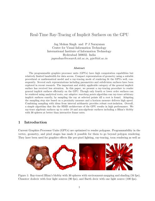
Technical Report: IIIT/TR/2007/72 3idea is to reduce the surface S(x,y,z) = 0 to the form F f (t) = 0 using the ray equation for thefragment f, where t is the ray-parameter. Each fragment can then solve for t and perform per-pixellighting, shadowing, etc., based on the exact intersection. Solution to the equation F f (t) = 0 dependson its form. Interactive ray-tracing has been achieved only for simpler implicit forms. These includealgebraic surfaces up to order 4 using analytical roots on the GPU [23] and selected algebraic surfacesup to order 6 and some non-algebraic surfaces using interval-analysis on the SSE hardware [20].Contributions <strong>of</strong> the paper: We introduce two ray-tracing algorithms that sample the ray to findan interval containing the intersection with the surface. The marching points algorithm that sampleseach ray uniformly in t to find solutions <strong>of</strong> the equation S(x,y,z) = S(p(t)) = 0 and the adaptivemarching points that samples each ray non-uniformly based on the distance to the surface and thecloseness to a silhouette. These methods have the flavour <strong>of</strong> brute-force linear searching but arefast due to the low computational requirements and better match with the SIMD architecture <strong>of</strong> theGPUs. They can also handle arbitrary implicit surfaces easily, needing only to evaluate S(x,y,z) atthe sample points. In fact, a key finding <strong>of</strong> this paper is that simple and seemingly non-promisingalgorithms that suit the architecture well can deliver very high performance on the GPUs. We alsopresent a root-containment test that combines the simplicity <strong>of</strong> ray sampling with the robustness <strong>of</strong>interval analysis using a first-order Taylor expansion <strong>of</strong> the function. This results in a fast, versatile,and robust ray-tracing scheme. We ray-trace algebraic surfaces <strong>of</strong> order up to 18 and non-algebraicsurfaces like super-quadrics, sinusoids, and blobbies with exact lighting and shadowing at significantlybetter than real-time rates. Figure 1 presents some <strong>of</strong> the surfaces ray-traced using our method.Additionally, we present fast ray tracing <strong>of</strong> algebraic surfaces <strong>of</strong> order less than five using closed-form,analytic solutions at higher frame rates – exceeding 1000 per second on an Nvidia 8800 GTX – thanreported before. We also present the first adaptation <strong>of</strong> the Mitchell’s interval-based method to theGPU using exact interval extension and ray trace algebraic surfaces <strong>of</strong> order less than 6 at frame ratesthat are at least an order <strong>of</strong> magnitude more than reported before.Section 2 reviews the previous work related to the topic <strong>of</strong> this paper. Section 3 presents oursampling based methods that provide speed and versatility. GPU implementations <strong>of</strong> analytic rootfinding and interval-based root-finding are presented in Section 4. Results <strong>of</strong> our algorithm on differentalgebraic and non-algebraic surfaces is presented in Section 5. Section 6 presents a comparison and adiscussion on ray-tracing on the GPUs and the CPU. Conclusions and directions for future work arepresented in Section 7. Appendix A presents the equations <strong>of</strong> the implicit surfaces used in the paperalong with simple screenshots.2 Related WorkWe review the related work divided into four sections: root finding for general functions, renderingimplicit surfaces, ray-tracing implicit surfaces, and ray-tracing on the GPU.Root Finding: Iterative root finding methods are used widely to solve general implicit equationsin one variable. Analytical solutions exist for polynomials <strong>of</strong> order four or lower; only iterative solutionsexist for higher order polynomials [3, 4] and other implicit forms. Iterative methods critically

Technical Report: IIIT/TR/2007/72 4depend on good initialization <strong>of</strong> the roots, which is difficulty for complex equations. An alternativeto initialization is to bracket the roots to an interval in t [33, 37] and then solve it using an iterativetechnique. Newton-Raphson, Newton-Bisection, and Laguerre’s method are popular for ray tracing[33, 18, 26, 52]. Extensions <strong>of</strong> these to use interval arithmetic have also been used [14, 21], which aremore robust at critical regions. Auxiliary polynomials [39] and Sturm sequences [49, 29] have also beenused to find roots <strong>of</strong> polynomials <strong>of</strong> various degrees. Most <strong>of</strong> these methods cannot be implementedeasily on the SIMD architecture <strong>of</strong> the GPUs, however.Rendering <strong>Implicit</strong> <strong>Surfaces</strong>: Polygonization can convert implicit surfaces into triangulated modelprior to rendering them using traditional graphics [5]. The marching cubes algorithm can be usedto create polygonal models from implicit functions [25]. Green et al. released a high-performance,marching tetrahedra package on the GPU recently [12], which can be used to polygonalize and renderarbitrary surfaces. In practice, this method is much slower than our approach and does not producegood results on complex surfaces due to severe resolution problems (Section 5.4). Twinned mesheswere introduced recently to triangulate dynamic implicit surfaces with changing topology using amechanical mesh and a geometric mesh [6]. Point or particle-based sampling and rendering <strong>of</strong> implicitsurfaces have also been popular [50, 46]. They distribute particles on the surface and applyattractive and repulsive forces to distribute them evenly on the surface. These methods are typicallydemonstrated on metaball or blobby surfaces used widely for fluid simulations and do not extend toarbitrary implicit surfaces well. Triangulation and point-sampling go against the strengths <strong>of</strong> the GPUby increasing the size and the bandwidth needs <strong>of</strong> the representation.<strong>Ray</strong>-<strong>Tracing</strong> <strong>Implicit</strong> <strong>Surfaces</strong>: <strong>Ray</strong>-tracing <strong>of</strong> implicit surfaces is about finding the smallestpositive root <strong>of</strong> an appropriate equation in the ray-parameter t. Hanrahan demonstrated ray tracing<strong>of</strong> algebraic surfaces up to the fourth order using Descartes rule <strong>of</strong> signs for root isolation and Newton’sbisection for root refinement [13]. Kajiya reduces ray tracing <strong>of</strong> spline surfaces to a globally convergentmethod resulting in root finding <strong>of</strong> an 18th degree polynomial using the Laguerre’s method [18].Interval-analysis has also been used for robust root isolation by many [27, 10, 7, 38, 11, 20]. Theinterval extension <strong>of</strong> a function gives a bound in its range given an interval in its domain. Mitchellisolates the root using repeated bisections till the interval in t contains a single root. Reliable intervalextensions,however, are difficult to compute for large intervals in the domain <strong>of</strong> complex functions.Subintervals, branch and bound schemes, octree grids, etc., have been used to increase the reliability <strong>of</strong>interval-based methods. Sherstyuk ray traces implicit surfaces by approximating F f (t) using piecewiseHermite polynomials <strong>of</strong> order 4 or lower and solving them using analytical methods [41]. Snyder posesproblems including ray tracing implicit surfaces and CSG as constraint minimization and performs anumerically stable global minimization using an interval analysis based method [43]. These resultshave been on the CPU mostly and involve low-order algebraic surfaces or small blobbies. Knoll etal. achieve 30 fps on a superquadric and 6 fps on a few sextic surfaces using the CPU and the SSEhardware [20]. The interval-based methods can be adapted to the GPU for faster ray tracing, as weshow in Section 4.2, but are limited in scope due to the difficulty <strong>of</strong> reliable interval extensions forhigher order algebraic and non-algebraic surfaces. Simple methods that suit the GPU deliver highperformance on them.

Technical Report: IIIT/TR/2007/72 5Sampling points along the ray and looking for intersections is a simple and intuitive way to isolatethe smallest positive root. This approach has been used for procedural hypertextures [30] and otherimplicit surfaces [19, 15]. Kalra and Barr ray-traced LG-implicit surfaces using Lipschitz constants, Lfor the function S(x,y,z) and G for its derivative along the ray F ′ (t), for efficient sampling <strong>of</strong> the rays[19]. Hart used variable step sizes in sphere tracing based on a geometric distance function evaluatedat the current point [15]. The Lipschitz theory or geometric distances do not extend easily to complexsurfaces, however. Our algorithms also follow the point sampling approach, but change the step sizeusing simpler measures that suit the GPU than optimal ones from Lipschitz theory.<strong>Ray</strong>-<strong>Tracing</strong> on the GPU: The traditional ray-tracing technique has been adapted to the GPU forgeneral polygonal models. Purcell et al. performed multipass ray tracing [34] and Carr et al. combinedCPU and GPU computations for a variety <strong>of</strong> tasks including recursive ray tracing [8]. These methodswork for general objects but are slow. Non-linear beam tracing on the GPU was demonstrated byLiu et al. for regular geometry [22]. Spheres and other quadric primitives were ray-traced on theGPU using per-fragment ray-quadric intersection and optimized bounding boxes [45, 42, 35]. Loopand Blinn showed resolution independent rendering <strong>of</strong> quadratic and cubic-spline curves on the GPU[24] and extended it to render piecewise algebraic surfaces up to fourth order defined over tetrahedralbases using analytical roots [23]. Bajaj et al. used cubic A-patches using Bernstein-Bezier bases withina tetrahedron as a way to approximate scattered points [2]. Seland and Dokken rendered algebraicsurfaces up to order five on the GPU [40] by computing the blossom <strong>of</strong> the function with respect toeach ray as a univariate Bernstein polynomial. This will not extend easily to higher order surfaces asthe complexity <strong>of</strong> computing coefficients <strong>of</strong> the univariate polynomial increases rapidly with its degree.Our method keeps the process simple to match the GPU by not evaluating the complex univariatepolynomials.Our Work in Context: The ray sampling methods we present (Section 3) steps along each ray tilla step covers a root. Step size is adapted using the algebraic distance to the surface and the angle theray makes with the local normal so that smaller steps are taken in regions that need greater attention.For robustness, we use simple interval analysis to test root-containment. Evaluating the multivariateS(x,y,z) polynomials instead <strong>of</strong> the complex and ray-dependent univariate F(t) polynomials reducesthe computation effort per pixel. The methods also work on arbitrary implicit surfaces since onlysamples <strong>of</strong> it are needed. The simplicity <strong>of</strong> the methods is the key to achieving high performanceon the restricted parallel architecture <strong>of</strong> the GPU. We can ray-trace algebraic surfaces up to order18 and several non-algebraic surfaces at framerates upwards <strong>of</strong> 100. The method works on dynamicimplicit surfaces also as the equation is evaluated directly in each frame with no precomputations.The analytical root-finding and Mitchell’s interval-based method are adapted to the GPU (Section4). The analytical roots are computed directly on the GPU without subdivisions and achieve fasterray-tracing framerates on quartics and cubics than reported before. We present the first interval-basedray-tracing on the GPU with an exact interval-extension, which can ray-trace algebraic surfaces upto order 5 without any subdivisions or octrees and achieves frame-rates that are at least an order <strong>of</strong>magnitude higher than reported previously.

Technical Report: IIIT/TR/2007/72 63 Marching Points and Adaptive Marching PointsThe fragment processors do most <strong>of</strong> the work in GPU-based ray-tracing. The ray parameters and thesurface equation are needed at each fragment shader program. The points on the ray for a fragmentf are given in the parametric form by P = O + tD f , where t is the ray parameter, O the cameracenter, and D f the direction <strong>of</strong> the ray. Substituting for x,y,z from the ray equation into the surfaceequation S(x,y,z) = 0, we getF f (t) = 0. (1)The smallest, real, positive solution for t gives the point <strong>of</strong> intersection <strong>of</strong> the ray with the object.Each fragment shader can independently find the root using a suitable method. The normal <strong>of</strong> thesurface at the point <strong>of</strong> intersection can also be computed as the gradient ⃗ ∇S(x,y,z) for exact lightingand shadows.3.1 Iterative Root-Finding: OutlineClosed-form, analytic roots <strong>of</strong> F f (t) exist only for algebraic forms <strong>of</strong> order less than five [4] and forsome non-algebraic forms. Root finding is quick, involving a few calculations per ray for such surfacesas we show in Section 4.1. Most interesting surfaces do not admit closed-form solutions and must besolved iteratively. Iterative methods need to be used with caution on implicit surfaces as the equationF f (t) may have many solutions. Standard iterative methods like Newton-Raphson, Laguerre, etc.,need good initialization for convergence. A two-step process with root isolation followed by rootrefinement works better in the general case. Root isolation returns a bracket or interval in the domainin which a root is present. Root refinement isolates the root within that bracket. The total searchrange is [t s ,t e ], the intersection <strong>of</strong> the ray with the near and far planes.Algorithm 1 Root-Finding: Overview1: Isolate the first interval [t 1 ,t 2 ] that contains a root for the ray corresponding to each fragment f.2: Refine the root in [t 1 ,t 2 ] using repeated bisections.We present two root isolation methods in this section based on sampling the ray and anothermethod in the next section based on interval analysis. A simple bisection method is used to refine theisolated root in all cases. The bisection method divides the given bracket [t 1 ,t 2 ] into two sub-intervals[t 1 ,t m ] and [t m ,t 2 ] using the midpoint t m . The smaller half that contains the root is identified andexplored further recursively. We perform 10 bisections after root isolation, but a condition based onthe value <strong>of</strong> |F f (t)| can be used instead. Bisection method is robust and succeeds in all cases, if thebracketing is correct [33]. It also guarantees that the solution gets closer to a real root with moreiterations. Other iterative methods (like the Newton-Raphson method) that base the next estimateon the secant or the gradient converge faster in theory than the bisection method. However, they arecomputationally more expensive due to need for derivatives and do not suit the SIMD computationmodel <strong>of</strong> the GPUs well. In practice, the root refinement step is less critical for all surfaces. In ourexperience, only about 15% <strong>of</strong> the total time is spent on the second step for all surfaces with thepercentage dropping below 10% for higher order algebraic surfaces.

Technical Report: IIIT/TR/2007/72 73.2 Computing S(x, y, z) vs F f (t)Root finding may need the values <strong>of</strong> the function F f (t) and possibly the first derivative Ff ′ (t) andhigher order ones at several points. The function can be evaluated for a given t using the univariatepolynomial F f (t) directly or using the multivariate polynomial S(x,y,z) = S(p(t)) after computing(x,y,z) = p(t) from t using the ray equation. The computational implications <strong>of</strong> each could be verydifferent. The expression F f (t) typically has many terms for higher order polynomials. Note that thecoefficients <strong>of</strong> F f () depend on the viewpoint and the pixel coordinates and cannot be precomputed.For example, a single sixth order expression x 3 y 3 <strong>of</strong> S() maps to (a+bt) 3 (c+dt) 3 in F f (t) and expandsto 16 terms for the 7 coefficients <strong>of</strong> the sixth order polynomial in t, requiring 44 multiplications and9 additions to evaluate. On the other hand, x and y can be computed using 2 multiplications and2 additions and x 3 y 3 can be evaluated using 5 more multiplications. The Barth decic (Section 5)can be evaluated using about 30 terms as S(x,y,z) but needs to evaluate 1373 terms to computeall 11 coefficients <strong>of</strong> the tenth order polynomial F f (t). The derivative Ff ′ (t) can also be calculatedefficiently using the gradient <strong>of</strong> S() as ∇S(x,y,z) ⃗ · D f . The univariate expression for the derivative isas cumbersome as the expression for F f (t).Loop and Blinn use GPU’s interpolation hardware to evaluate the coefficients <strong>of</strong> the polynomial[23]. They evaluate the polynomial using a tensor contraction in a Bezier-Bernstein tetrahedral basis.This is achieved by sending a symmetric tensor <strong>of</strong> rank d − 1 with ( d+2d−1)unique elements from thevertex shader for each <strong>of</strong> the 4 vertices <strong>of</strong> the tetrahedra. The rasterization hardware on the GPUinterpolates the tensor values after which, the fragment shader computes the coefficients efficientlyusing dot products. While this method is very clever, it will be computationally expensive for higherorderpolynomials as O(d 3 ) elements need to be sent for an algebraic surface <strong>of</strong> order d. This willalso not extend easily for other non-algebraic surfaces. Since their goal was to render piecewise loworder algebraic objects, streaming the coefficients down the pipeline was essential and delivered decentspeed.A balanced computation load is critical to good performance on the GPUs, given their SIMDmodel and limits on the length <strong>of</strong> the shader programs. Methods that use the S(x,y,z) values arelikely to be faster than those that use F f (t) values. Root finding schemes that use Bezier-Bernsteinbases, Sturm sequences, singular value decomposition <strong>of</strong> the companion matrix, etc., operate primarilyin the space <strong>of</strong> the F f (t) polynomial and will be quite inefficient on the GPU for higher order surfaces.3.3 Marching Points AlgorithmShort and simple computations achieve the best performance on GPUs. An exceedingly simple rootisolationscheme is to march a point along the ray till the function F f (t) crosses zero between twosamples. The point needs to march between bounds in t given by the view frustum or the boundingvolume <strong>of</strong> the object. The computation complexity is low as only F f (t) = S(p(t)) needs to be evaluatedat the sample points. This suits the SIMD model <strong>of</strong> the GPU and can exploit its high computingpower. We call this the marching points (MP) algorithm (Algorithm 2). This algorithm can be usedfor arbitrary implicit surfaces, even those with difficult derivatives or for general piecewise algebraicsurfaces without derivatives at boundaries. The performance <strong>of</strong> the algorithm depends on the marching

Technical Report: IIIT/TR/2007/72 8y = F(t)psy = F(t)Eyeqy = 0rABCFigure 2: Marching points algorithm samples uniformly in the ray parameter t. The sign test identifiesthe first interval where the function changes sign at the endpoints (darker shaded region on the left).Sign test will fail as the step size increases (right). Roots will be isolated in intervals [A, B] and [B, C].If the step size doubles again, the roots in [A, C] will be missed by the sign test. Taylor test detectsthe root in [A, C] by including points q and r into the calculations.or sampling step-size. The optimal step-size may differ from one surface to another.Algorithm 2 Marching Points (f,N)1: Find the bounds t s and t e <strong>of</strong> the ray for fragment f.2: Divide [t s ,t e ] into N equal intervals3: for i = 0 to N − 1 do4: if rootExistsIn (t i ,t i+1 ) then5: Return [t i ,t i+1 ] as containing a root6: end if7: end forThe root-containment test used in step 4 is the critical operation in the above procedure. The testcan be implemented in different ways. Two promising root-containment tests are the following.1. Sign test: rootExistsIn (t i ,t i+1 ) = (S(p(t i ))∗S(p(t i+1 )) < 0). Root exists if the function changessign between the end points <strong>of</strong> the step. This test is simple to implement as only the functionvalues at the sample points are needed. It is also a strict test that does not produce false roots.It may, however, miss roots if an even number <strong>of</strong> roots are in the step.2. Taylor test: rootExistsIn (t i ,t i+1 ) = (0 ∈ ˜F([t i ,t i+1 ])), a test for containment <strong>of</strong> a zero withina step. Interval arithmetic gives bounds <strong>of</strong> functions for a range in its domain as seen earlier.Exact interval extension is impractical in general, but acceptable ones can be found if the intervalis small enough. We use an interval extension employing the function values at the endpoints aswell as the first order Taylor series approximation <strong>of</strong> the function at the middle <strong>of</strong> the intervalcomputed from both endpoints (Figures 2 and 7). This works adequately for moderate lengths<strong>of</strong> intervals. The interval extension in the interval [t i ,t i+1 ] is defined as˜F([t i ,t i+1 ]) = [min {p,q,r,s}, max {p,q,r,s}]wherep = F(t i ), q = F(t i ) + F ′ (t i ) (t i+1 − t i )2, r = F(t i+1 ) − F ′ (t i+1 ) (t i+1 − t i ), s = F(t i+1 ). (2)2

Technical Report: IIIT/TR/2007/72 9This test is slower than the sign test because <strong>of</strong> the derivatives but larger step-sizes can beused. In practice, the running time doesn’t change much on the average though the higher ordersurfaces suffer more due to the derivative calculations. This test can produce false roots, butworks robustly in practice and can handle multiple roots well.The worst case running time <strong>of</strong> marching points is linear in the size <strong>of</strong> the total range in t. However,it is fast in practice and can render a large number and type <strong>of</strong> surfaces. Table 1 gives the runningtime performance for algebraic surfaces up to order 18 and for several non-algebraic surfaces usingboth tests. The step-size is chosen so as to not miss any root. The interval [t s ,t e ] is divided equallyinto the number <strong>of</strong> steps shown the table, ranging from 25 to 400 steps. Algebraic and non-algebraicimplicit surfaces as complex as these have never been ray-traced at interactive rates before to the best<strong>of</strong> our knowledge.Surface Max Frames per second Surface Max Frames per second[order] steps Sign Taylor [order] steps Sign TaylorAlgebraic <strong>Surfaces</strong>Chmutov [18] 400 85 38 Kleine [6] 400 285 290Chmutov [14] 400 55 48 Dervish [5] 300 285 275Sarti [12] 300 60 53 Peninsula [5] 85 370 447Barth [10] 300 92 105 Piriform [4] 55 520 305Chmutov [9] 200 125 135 Cushion [4] 75 390 305Endrass [8] 300 140 179 Torus [4] 50 410 430Chmutov [8] 250 185 195 Cassini [4] 55 405 375Chmutov [7] 175 138 206 Cross-Cap [4] 50 400 465Labs [7] 200 115 120 Goursat [4] 50 580 515Barth [6] 125 300 310 Cayley [3] 60 460 475Heart [6] 120 265 260 Clebsch [3] 55 470 500Hunt [6] 400 230 225 Ding-Dong [3] 25 825 560Non-Algebraic <strong>Surfaces</strong>Superquadric 150 105 125 Scherk’s 250 200 315Blobby 250 160 305 Diamond 250 260 306Blinn’s Blobby 75 380 460Table 1: Maximum number <strong>of</strong> steps and the frame rate using the marching points method for a512 × 512 window.3.4 Adaptive Marching Points AlgorithmThe marching points algorithm takes fixed size steps in empty space as well as near the surface. Thestep-size has to be small enough to handle the worst-case, which occurs near the silhouette <strong>of</strong> thesurface. Larger step-sizes suffice in empty space if small step sizes can be used close to the surface.The adaptive marching points (AMP) algorithm uses a step size that depends on the closeness <strong>of</strong>the point to the surface and to its silhouette. We need a proximity measure to determine how close

Technical Report: IIIT/TR/2007/72 10the current point on the ray is to the surface and a horizon measure to determine how close it is toa silhouette <strong>of</strong> the surface. The step-size should be small when near the surface and smaller nearsilhouettes.EyeIVVIIIIIτ 3τ 2τ 1IS(x, y, z) = 0Figure 3: Adapting the step size to the distance to the surface. Region IV will have the largest stepsize and the region I will have the smallest, based on the proximity measure |S(x,y,z)|. The stepsize is further reduced for when the horizon condition is true (the darkened region V) as the surfacenormal is nearly perpendicular to the viewing direction.Geometric distances are reliable measures <strong>of</strong> proximity to a surface. They are, however, surfacedependent and not available for arbitrary implicit surfaces. Lipschitz bounds can be used to estimatethe optimum step size for efficient ray-tracing [19, 15]. The Lipschitz constant can be defined as themaximum absolute value <strong>of</strong> a the derivative <strong>of</strong> the function in an interval. Unfortunately, it is hard tocompute for the higher order algebraic and general implicit surfaces. Taubin suggests the use <strong>of</strong> theratio F(t)|F ′ (t)|as a measure for signed geometric distance to the function F(t) [44]. However, the measureis useful only for low-order algebraic surfaces and for points close to the surface. Most areas <strong>of</strong> thesurface are missed on most higher-order surfaces with this distance function, in practice. Extendingthe definitions for geometric distance and Lipschitz bounds to arbitrary algebraic and non-algebraicsurfaces will be a fruitful research direction for the future.Algorithm 3 Adaptive Marching Points (f,b)1: Find the intersections t s and t e <strong>of</strong> the ray for fragment f with the near and far planes.2: Initialize s to the basic step size b; t to starting point t s3: while⎧t < t e dob/4 if |S(p(t))| ≤ τ 1 and | ∇S(p(t)) ⎪⎨⃗ · D f | ≤ ǫb/2 if |S(p(t))| ≤ τ4: s =12b if |S(p(t))| > τ ⎪⎩2b otherwise5: if rootExistsIn (t,t + s) then6: Return [t,t + s] as containing a root7: end if8: t = t + s9: end whileThe magnitude <strong>of</strong> S(x,y,z) gives the algebraic distance from a point to the surface. We use itas the proximity measure and vary the step-size as a monotonic function <strong>of</strong> it. In practice, we usea piecewise constant approximation <strong>of</strong> this function and vary the step size in octaves, starting with

Technical Report: IIIT/TR/2007/72 11Surface Max Frames per second Surface Max Frames per second[order] steps Sign Taylor [order] steps Sign TaylorAlgebraic <strong>Surfaces</strong>Chmutov [18] 100 98 60 Kleine [6] 48 435 385Chmutov [14] 100 125 95 Dervish [5] 45 285 280Sarti [12] 100 86 75 Peninsula[5] 35 512 435Barth [10] 100 150 115 Piriform [4] 32 552 315Chmutov [9] 81 185 165 Cushion [4] 32 420 335Endrass [8] 96 190 208 Cassini [4] 32 525 506Chmutov [8] 64 215 216 Cross-Cap[4] 32 530 540Chmutov [7] 63 242 233 Torus [4] 24 555 525Labs [7] 77 232 310 Goursat [4] 24 635 605Hunt [6] 84 240 325 Cayley [3] 33 600 652Barth [6] 60 325 310 Clebsch [3] 21 585 555Heart [6] 48 420 325 Ding-Dong[3] 15 920 665Non-Algebraic <strong>Surfaces</strong>Superquadric 100 185 155 Scherk’s 100 358 322Blobby 50 329 300 Diamond 100 360 330Blinn’s Blobby 40 456 545Table 2: Maximum number <strong>of</strong> steps and the frame rate using the adaptive marching points methodfor a 512 × 512 window.a base step size <strong>of</strong> δ. The base step size is multiplied by 2 if the current point is far away from thesurface and halved if close to it, using two thresholds τ 1 and τ 2 . Thus, different step sizes can be usedin regions <strong>of</strong> different colour/shade shown in Figure 3. The same base step as the marching pointsalgorithm is used and the thresholds are set based on the coefficients <strong>of</strong> S().It is also important to adapt the step-size to the view-dependent silhouettes. We decrease thestep-size near the silhouettes <strong>of</strong> the surface, using |Ff ′ (t)| as a horizon measure. Note that the compleximplicit surfaces may have many internal silhouettes that need to be handled carefully. We use|Ff ′ (t)| ≤ ǫ as a horizon condition, which works fine for surfaces with continuous gradients. This is areliable horizon measure if p(t) is close to the surface, being the cosine <strong>of</strong> the angle between the ray andthe local surface gradient. The step size is reduced near the silhouettes based on |Ff ′ (t)|. In practice,we halve the step-size further when the horizon condition is met (Algorithm 3). Thus, the darker, ovalregion <strong>of</strong> Figure 3 will have further reduced step sizes in order to render silhouettes well. The use <strong>of</strong>multiple thresholds ǫ 1 ,ǫ 2 , and additional piecewise constant levels can provide greater adaptation todifficult silhouettes, but the single threshold suffices in practice for the kind <strong>of</strong> surfaces we dealt with.Olievera et al. also used the angle between the viewing direction and the surface normal to controlthe step size while ray-tracing height-fields on the GPU [32, 31].Marching points and adaptive marching points can, however, miss multiple roots or produce falseroots based on the specific test used, as explained earlier. A comparison <strong>of</strong> different tests for multipleroots is shown in Figure 6. The sign-change test can miss the root when the interval contains multiple

Technical Report: IIIT/TR/2007/72 12Figure 4: Top row: Barth tenth order surface without silhouette adaptation (left) and with it (right).The zoomed views in the middle show great reduction in the aliasing for the internal silhouettes.Bottom row: Superquadric surface without (left) and with (right) silhouette adaptation with zoomedviews in the middle.Figure 5: Number <strong>of</strong> steps taken along each ray for a Barth tenth order surface. Darker green indicatesfewer steps. The red rays didn’t intersect the surface and incurred the maximum amount <strong>of</strong> work.Left: marching points, right: complete adaptive marching points, middle: AMP without silhouetteadaptation.roots. We can <strong>of</strong>fset the surface by a small value to render S(x,y,z) = ǫ to alleviate proble (Figuer 6).Strictly speaking, we are rendering a different surface, but the results can be close enough. Offsettingis similar to the S(x,y,z) ≤ ǫ test for roots used by sphere tracing [15]. The Taylor test usign thefirst order interval extension produces robust results similar to the interval-based method given inSection 4.2 (Figure 6), confirming that it is a decent interval extension method in small intervals.The adaptive marching points method (Algorithm 3) achieves better rendering speeds without losingthe versatility or quality <strong>of</strong> the basic marching points method (Table 2). Figure 4 shows the effect<strong>of</strong> silhouette adaptation. The aliasing at the silhouettes reduces sharply with silhouette adaptation.The superquadrics have the most challenging silhouettes as the surface is not C 1 continuous. Thealiasing effects can be seen occasionally on these surfaces on the video. Figure 5 shows the number<strong>of</strong> iterations used for each pixel as a measure <strong>of</strong> the work done for the Barth decic surface. Adaptivemarching points does less work than marching points almost everywhere. The extra effort near thesilhouettes can be observed when silhouette adaptation is used.

Technical Report: IIIT/TR/2007/72 13Figure 6: Top row: Steiner, Cross Cap, Miter and Kiss surfaces ray-traced using the adaptive marchingpoints method with the sign test. Multiple roots are missed by it. Second row: <strong>Surfaces</strong> shifted by 0.01using AMP and sign test. Region <strong>of</strong> multiple roots tend to be fattened. Third row: Same surfacesrendered using the AMP algorithm and the Taylor test for root containment. The performance ismore robust for multiple roots. Bottom row: Same surfaces rendered using Mitchell’s interval-basedmethod (Section 4.2) which also produces robust roots.4 GPU <strong>Ray</strong>-<strong>Tracing</strong> using Analytic Roots and Interval AnalysisIn this section, we present the GPU implementation <strong>of</strong> two previously reported methods: exact rootfinding using analytical methods and Mitchell’s root isolation method using interval-analysis.4.1 Closed-Form, Analytic Root-FindingAnalytic solutions to Equation 1 exists only for simple forms <strong>of</strong> F f (), such as polynomials <strong>of</strong> orderless than five. Root-finding for quadric surfaces have been used for ray-tracing [45, 42, 35]. Resultson cubics and quartics have been reported using tetrahedral bases to limit the search range for theroots [23].We solve the cubic equation using the method given by Blinn [3, 4]. For a cubic equation Ax 3 +3Bx 2 w + 3Cxw 2 + Dw 3 = 0, compute δ 1 = AC − B 2 , δ 2 = AD − BC, and δ 3 = BD − C 2 . Thediscriminant is defined as ∆ = 4δ 1 δ 3 −δ 2 2 . The sign <strong>of</strong> the discriminant and the values <strong>of</strong> δ is determineif it has one triple root, one double and a single real root, three distinct real roots, or one real root

Technical Report: IIIT/TR/2007/72 14and one complex conjugate pair as roots. These can be worked out for each fragment independentlyfor fast rendering <strong>of</strong> the shapes. We are able to achieve over 3000 fps on cubics as shown in Table 3.We use the Ferrari method described by Herbison-Evans for the fourth order polynomials [16].The equation is first depressed by removing the cubic term to the form t 4 + pt 2 + qt + r = 0. If r iszero, the roots are 0 and the roots <strong>of</strong> the cubic equation. If r is non-zero, the equation can be writtenas a product <strong>of</strong> two quadric equations. This is done by rewriting it as (t 2 + p) 2 + qt + r = pt 2 + p 2 .This is followed by a substitution y such that the right hand side (RHS) becomes a perfect square.The equation then transforms to (t 2 + p + y) 2 = (p + 2y)t 2 − qt + (y 2 + 2yp + p 2 − r). Now, for theRHS to be a perfect square its discriminant must be zero which leads to a cubic equation in y whoseroot is found as described before.Surface FPS Surface FPSSteiner Quartic 1400 Miter Quartic 1045Torus Quartic 1200 Cross Cap Quartic 1025Tooth Quartic 1100 Clebsch Cubic 3400Goursat Quartic 1175 Cayley Cubic 3300Cassini Quartic 1103 Ding-Dong Cubic 3750Piriform Quartic 1082Table 3: Frame rates for different surfaces using analytic root-finding for a 512 × 512 window on anNvidia 8800 GTX.Table 3 shows the frame rates for representative cubic and quartic surfaces for a resolution <strong>of</strong>512×512 on an Nvidia 8800 GTX. Techniques specialized for spheres or ellipsoids achieve 15-30 fps ona scene with 99K tiny spheres but do not give the rendering time <strong>of</strong> a single primitive [42, 35]. Loopand Blinn report an fps <strong>of</strong> 1200 on single quadratics and about 500 on single quartics. Our results are2-4 times faster than theirs on a 8800 GTX compared to the 7800 GTX they used. While most quarticswork perfectly, surfaces with self intersections or multiple roots like Steiner, Cross-Cap, and Miter,have small holes from a few viewpoints. Multiple roots are hard for root-finding methods in general.The analytical methods may be able to detect degenerate situations based on the determinants andtake suitable action.4.2 Interval-Based Root IsolationInterval-based methods have been used for robust root-finding [1, 28]. The basic idea is to extend afunction to an interval in its domain, with the result being an interval in its range. If ˜x is an interval[a,b], the interval extension ˜f(˜x) is an interval [p,q] that encloses the minimum and maximum values<strong>of</strong> f(x) for x ∈ [a,b]. Interval extensions <strong>of</strong> iterative root-finding methods produce more robust rootsbecause they don’t deal with possibly singular values.Mitchell’s algorithm for root finding recursively isolates an interval that contains the root by halvingit, using interval arithmetic [27]. The interval extension <strong>of</strong> the function F f (t) and its derivative F ′ f (t)are used for this. If the interval extension <strong>of</strong> the function does not contain 0, then the correspondinginterval does not have a root inside the interval. The interval contains one or more roots otherwise.

Technical Report: IIIT/TR/2007/72 15If the interval extension <strong>of</strong> its derivative does not contain 0, then the function is monotonic in theinterval and contains a single root. Otherwise (i.e., the interval extensions <strong>of</strong> the function and itsderivative contain 0), the function has multiple roots in the interval. The interval is then bisected andthe procedure is applied on both intervals recursively, starting with the lower half.We adapted this algorithm for the GPU for root isolation (Algorithm 4). Since we are interestedin the smallest positive real root, we check the second half <strong>of</strong> the interval only if the first does notcontain a root. Algorithm 4 is executed on the GPU independently for each ray. We exploit the vectoroperations <strong>of</strong> the GPUs to implement interval arithmetic operations. The bisection at each step resultsin a running time that is logarithmic in the length <strong>of</strong> the starting interval. We render several algebraicsurfaces <strong>of</strong> order up to 5 and a few non-algebraic surfaces using the above algorithm. Table 4 showsthe frame rate achieved on different surfaces. The average number <strong>of</strong> iterations vary from 18 for theDing Dong cubic to 85 for the Dervish quintic using this method. The rendering speed is affected bythis, but better than interactive rates is achieved on all these surfaces. The previous interval basedmethods on the CPU were limited to 4th order algebraic surfaces, superquadrics, Steiner surface,and blobbies. Recently, a sixth order surfaces was ray-traced at 6 fps and a superquadric at 30 fpsusing the CPU plus the SSE hardware [20]. Ours is the first reported attempt at implementing theinterval-based ray tracing on the GPUs.The effectiveness <strong>of</strong> interval-based methods depends critically on the interval extension used. Findingthe bounds in range <strong>of</strong> a function given an interval in its domain is a hard problem for arbitraryfunctions. Figure 7 illustrates the difficulty involved. Common methods like the natural and thecentered interval extension [17] use the values <strong>of</strong> the function and/or its derivative at both ends <strong>of</strong> theinterval. These can miss the root if an even number <strong>of</strong> roots are in the interval. Another option is tointerval extend each argument independently and evaluate the function using interval-based addition,subtraction, multiplication, etc. The bounds generated by this method tend to overestimate the truebounds and can result in false roots when the domain interval is large, as is well known [20].The bounds in the range <strong>of</strong> a function can be computed exactly only if all critical points in theinterval are known. For algebraic surfaces, this reduces to finding all roots <strong>of</strong> a polynomial <strong>of</strong> orderless by one. Consequently, we can only render algebraic surfaces <strong>of</strong> order 5 or less (Table 4). It shouldbe noted that rendering a quintic surface involves solving for all roots <strong>of</strong> a 4th order polynomial tocompute the interval extension <strong>of</strong> the function and solving for all roots <strong>of</strong> a 3rd order polynomial toAlgorithm 4 Interval-Based Root Isolation (f,a,b)1: Compute the interval extensions ˜F f ([a,b]) and ˜F ′ f [a,b].2: if 0 /∈ ˜F f ([a,b]) then3: Declare no root4: else if 0 ∈ ˜F f ([a,b]) and 0 /∈ ˜F f ′ ([a,b]) then5: Single root. Return [a,b]6: else if 0 ∈ ˜F f ([a,b]) and 0 ∈ ˜F f ′ ([a,b]) then7: Multiple roots. Invoke the algorithm for the interval [a, a+b2 ].8: If no root, invoke algorithm for [ a+b2 ,b].9: Until a root is isolated or the width <strong>of</strong> interval is less than ǫ.10: end if

Technical Report: IIIT/TR/2007/72 16iy = F(t)y = 0jktA B C DlFigure 7: Interval extension methods. Roots in ranges [A, B], [B, C], and [C, D] can be found usingthe natural extension involving the function values at the end points only, which will not work for [A,C] or [B, D]. The first-order Taylor expansion based extension can work for [A, C]. All critical points<strong>of</strong> the function need to be evaluated to detect the root in the range [B, D]. The first-order extensionsfor [A, C] are i and j and for [B,D] are k and l.do the same for its derivative, per fragment. Interval-based methods, thus, incur heavy computationsand achieve lower framerates as a result.The total interval [t s ,t e ] is typically too large in practice for bisections to work using an inexactinterval extension for complex surfaces. Subdivision <strong>of</strong> the interval can enable the reliable use <strong>of</strong>a simpler interval extension method. However, for arbitrary functions, such subdivision based on aproper analysis is difficult. The considerations are similar to those used in setting the optimal step-size<strong>of</strong> the marching points method. The Taylor series expansion based interval extension (Section 3.4) isone that works on smaller sub-intervals.5 ResultsIn this section, we present the complete rendering results on several algebraic and non-algebraicsurfaces. We could render algebraic surfaces up to order 18 including all surfaces shown in theMathWorld site and several non-algebraic and transcendental objects. Screenshots <strong>of</strong> these surfacesappear in Figures 12 and 13. The equations <strong>of</strong> the corresponding surfaces is given in the AppendixA. First, we display the overall ray-tracing algorithm and some <strong>of</strong> its implementation issues.5.1 Overall Algorithm: Implementation IssuesThe overall ray-tracing program for implicit surfaces is given in Algorithm 5. The implementationis in OpenGL/GLSL for the SM4.0 architecture <strong>of</strong> the Nvidia 8800 GTX GPU. Here we give a fewpoints to be kept in mind for efficiency and applicability.1. Analytical root-finding (Section 4.1) can be used for surfaces <strong>of</strong> order less than 5. Adaptivemarching points (Section 3.4) performs the best otherwise.

Technical Report: IIIT/TR/2007/72 17Surface No. <strong>of</strong> Frames Surface No. <strong>of</strong> Frames[order] iterations per second [order] iterations per secondDervish [5] 86 60 Nordstrands [4] 47 220Kiss [5] 65 77 Kummer [4] 45 225Peninsula [5] 60 85 Steiner [4] 45 235Cushion [4] 53 170 Piriform [4] 42 230Cross-Cap [4] 52 195 Torus [4] 32 400Miter [4] 52 186 Cayley [3] 27 580Tooth [4] 50 195 Clebsch [3] 25 590Cassini [4] 48 215 Ding-Dong [3] 18 965Goursat [4] 47 210Table 4: Number <strong>of</strong> iterations and the frame rate using the interval-based method for a 512 × 512window.2. The shaders are compiled on the fly under current programming environments including GLSLand Cg. The function to evaluate the expression S(p(t)) and its gradient (if necessary) can besynthesized on the fly by the CPU for the specific surface.3. Computing S(p(t)) and its gradient ⃗ ∇S(p(t)) together in one function is more efficient thanevaluating them separately as many calculations can be shared. The gradient is needed only insome cases, like the interval-based methods and for silhouette adaptation.4. Products <strong>of</strong> vectors are used to compute x 2 ,y 2 ,z 2 ,x 3 ,y 3 ,z 3 , etc., simultaneously within theshaders. Dot products are used wherever possible.5. All timing given in this paper are for ray-tracing all 512 × 512 rays <strong>of</strong> the screen. Simpleoptimizations involving bounding boxes <strong>of</strong> the objects, octree partitioning, etc., can increase thetiming performance greatly as reported earlier [19, 15]. Most <strong>of</strong> the complex surfaces are notbounded easily, however.6. The vertex and geometry shaders jointly perform initializations <strong>of</strong> the common parameters anddrawing a screen-sized quad. The root finding is performed on the fragment shader using singleprecision floating point arithmetic.5.2 Self ShadowingThough the single-bounce ray-tracing was described so far, secondary rays can be spawned from points<strong>of</strong> intersection for shadowing, reflections, transparency, etc. General recursive ray-tracing will requireextensive book-keeping to perform on the shader and will be difficult on the GPUs. Shooting secondaryrays to the light sources to compute per-pixel shadowing is practical, however. A point is shadowedif the ray from it to the light source hits the surface before the light source. We only need to know ifa point is shadowed; we needn’t know the intersection <strong>of</strong> the secondary ray with the surface. Thus,only root isolation (step 2 <strong>of</strong> Algorithm 1) is needed. Figures 1 and 8 show the shadowing effects on afew surfaces, including from multiple light sources. The video contains more interactive shots. Table

Technical Report: IIIT/TR/2007/72 18Algorithm 5 <strong>Implicit</strong>Surface Render (f)CPU:1: Setup equations in the shader program.2: Send a dummy quad to the OpenGL pipeline.Vertex Shader:1: Pass through vertices without any modification and camera center to the geometry shader.Geometry Shader:1: Transform the dummy quad to screen-facing quad and pass parameters like the ray direction tothe vertices, the camera center, near, and far plane distances to the pixel shader.Fragment Shader:1: Intersect each ray with the near and far planes to get the range [t s ,t e ].2: Isolate the root using one <strong>of</strong> the described algorithms.3: Refine the root using 10 steps <strong>of</strong> Newton’s Bisection method.4: Shoot a ray from the intersection point towards the light source(s). Perform root-isolation for it.If root is found, the point is under shadow.5: Compute per-pixel colour and depth using the position, normal, and shadowing at the intersectionpoint.5 shows the performance <strong>of</strong> each algorithm with and without shadows. The rendering rate suffers alittle due to shadowing, while comfortably being above the real-time rates in all cases.Figure 8: Chmutov octdecic, Chmutov quaddecic, Sarti dodecic, Kiss quintic, and a Blobby surfacewith self shadows and highlights.5.3 Rendering <strong>Time</strong>sTable 5 presents the comprehensive frame rates for all methods discussed in the paper on severalalgebraic and non-algebraic surfaces for both with shadow rays and without them on an Nvidia 8800GTX for a resolution <strong>of</strong> 512×512. The interval-based method has low applicability but shows the leastdrop in fps due to shadowing. Marching points and its adaptive versions are versatile and fast. Theyhave difficulty with surfaces with a long locus <strong>of</strong> multiple roots as explained earlier. The renderingtimes are orders <strong>of</strong> magnitude better than anything reported in the literature. We also report real-timeresults on surfaces much more complicated than have been reported before.

Technical Report: IIIT/TR/2007/72 19Interval Adaptive Marching Points AlgorithmSurface Based #Steps: Hand-Tuned #Steps: Fixed Formula[order] Algorithm Sign test Taylor test Sign test Taylor testA B A B A B A B A BAlgebraic <strong>Surfaces</strong>Chmutov [18] - - 98 70 60 45 98 70 45 38Chmutov [14] - - 125 95 95 75 125 95 66 59Sarti [12] - - 86 78 75 49 86 78 69 60Barth [10] - - 150 110 115 79 150 110 82 75Chmutov [9] - - 185 150 165 120 168 129 106 90Endrass [8] - - 190 140 208 140 185 135 133 105Chmutov [8] - - 215 175 216 161 165 160 145 110Chmutov [7] - - 242 180 233 175 200 164 158 125Labs [7] - - 232 165 310 155 220 150 125 105Chmutov [6] - - 418 280 325 235 265 225 165 133Hunt [6] - - 240 182 310 155 240 172 139 102Barth [6] - - 325 270 325 230 316 225 175 139Heart [6] - - 420 280 300 225 275 235 185 133Kleine [6] - - 435 267 385 245 285 240 195 165Dervish [5] 60 54 285 250 280 175 215 195 178 135Kiss [5] 77 71 428 325 435 265 405 295 270 230Peninsula [5] 85 78 520 326 535 295 380 285 306 235Steiner [4] 235 215 645 420 516 315 405 365 270 240Cassini [4] 215 208 510 320 506 285 396 305 285 240Tooth [4] 195 190 617 425 542 287 440 375 345 260Piriform [4] 230 222 552 450 315 246 345 275 291 240Cross-Cap[4] 195 188 530 305 540 285 325 265 251 215Miter [4] 186 176 535 325 528 285 345 285 245 225Kummer [4] 225 219 555 405 302 245 318 245 195 155Goursat [4] 210 198 635 420 605 325 420 365 315 265Cushion [4] 170 163 420 320 335 225 329 250 186 145Nordstrands [4] 220 211 458 305 324 235 336 285 245 170Cayley [3] 580 572 600 365 652 315 452 345 391 200Clebsch [3] 590 588 585 355 555 235 425 335 340 205Ding-Dong [3] 965 960 918 482 665 475 605 485 450 325Non-Algebraic <strong>Surfaces</strong>Torus - - 540 350 515 295 540 350 515 295Superquadric - - 185 145 155 105 185 145 155 105Blobby - - 329 265 300 195 329 265 300 195Blinn’s Blobby - - 456 344 545 325 456 344 545 325Scherk - - 358 222 322 185 358 222 322 185Diamond - - 360 208 330 199 360 208 330 199Table 5: Rendering time results for several algebraic and non-algebraic surfaces for different algorithms.Frame rates without shadows is given in A columns and with shadows is shown in B columns for a512 × 512 window on an Nvidia 8800 GTX. The order <strong>of</strong> each algebraic surface appears within squarebrackets. The timings on the left half for AMP are for step-sizes adjusted manually. The right halfuses a conservative formula (see Section 5.6) for the maximum number <strong>of</strong> iterations.

Technical Report: IIIT/TR/2007/72 20Surface FPS using FPS using[20] our methodTorus 22.9 555Kleine 6.0 435Barth Sextic 4.9 325Steiner1 6.1 639Steiner2 17.2 320Mitchell 5.9 425Tangle 3.8 483Absolute Value 30.8 379Teardrop 15.3 437Table 6: Comparison <strong>of</strong> frame rates for different surfaces using Knoll’s method on a CPU with SSEhardware and our AMP method on the GPU on common surfaces.5.4 Comparison with SSE <strong>Ray</strong>-tracing and Marching TetrahedraComplex implicit surfaces like the ones we used have not been ray-traced before on the GPUs toprovide comparison. The best reported effort by Knoll et al. achieve a frame rate <strong>of</strong> 15 on a quinticsurface, 6 on a sextic surface, and up to 30 on superquadric-like surfaces on a CPU with the SIMDextensions [20]. Our method is orders <strong>of</strong> magnitude faster as seen in Table 6. Since the GPU is afaster processor, the frame-rate comparison may not be meaningful. Their method involves an inexactinterval extension and may not extend to very high order algebraic surfaces. It is also not likely tobe as fast on the GPU as our methods as our own experience with the interval-based and marchingpoints methods.Surface Marching Marching Points Adaptive March. PtsName Tetrahedra 64 3 128 2 × 64 256 2 × 64 128 2 × 64 256 2 × 64DingDong [3] 14 0.468 0.810 0.445 0.751Steiner [4] 14 0.586 0.924 0.513 0.797Peninsula[5] 16 0.537 0.890 0.539 0.738Chmutov [7] 16 0.634 1.154 0.610 1.109Chmutov [8] 32 0.689 1.323 0.653 1.353Chmutov [9] 46 0.757 1.343 0.730 1.398Table 7: Rendering times in milliseconds for the GPU marching tetrahedra for 64 3 resolution andmarching points and adaptive marching points for 128 2 × 64 and 256 2 × 64 resolutions on an Nvidia8800 GTX.<strong>Implicit</strong> surfaces can, however, be polygonized using an algorithm like the Marching Cubes algorithm[25] as the iso-surface <strong>of</strong> S(x,y,z). An efficient implementation <strong>of</strong> the marching tetrahedramethod – a variation on the marching cubes – was made available recently for the GPUs by Nvidia[12]. It works in a voxelized space <strong>of</strong> resolution m×n×p and finds the triangles on the iso-surface.We adapted the code to render the triangles with per-pixel lighting and tried it on different implicitsurfaces. Table 7 lists the running times <strong>of</strong> marching tetrahedra and our method on comparable resolu-

Technical Report: IIIT/TR/2007/72 21Figure 9: Left to right: Steiner quartic surface rendered with marching tetrahedra and with adaptivemarching points. Hunt’s sextic surface with marching tetrahedra and adaptive marching points.Marching tetrahedra was computed for a 64 3 voxel grid and AMP for a 256 2 × 64 grid and renderedat a 256 × 256 resolution.tions and Figure 9 provides the visual rendering results. The 64×64×64 configuration <strong>of</strong> the marchingtetrahedra produces nearly the same visually quality as the 128×128×64 configuration <strong>of</strong> marchingpoints when rendering to a 128×128 window. We had difficulty getting higher resolutions <strong>of</strong> marchingtetrahedra to work on GPU. Our method is 20 to 50 times faster than marching tetrahedra. Themarching tetrahedra algorithm is also not able to handle more complex surfaces than those shown inthe table. The coarse sampling <strong>of</strong> marching tetrahedra also produces more artifacts on difficult areasas can be seen in Figure 9.5.5 Dynamic <strong>Implicit</strong> ObjectsA dynamic implicit object changes its form over time. The rayskip algorithm ray-traces dynamicimplicits by exploiting the temporal and spatial coherence <strong>of</strong> ray-implicit intersections [9]. Knoll etal. render dynamic implicits as 4D implicits in an (x,y,z,t) space [20]. The algorithms presented inthis paper ray-trace the implicit surface independently in each frame without any precomputations orsubdivisions. Thus, the equation can change each frame without affecting the performance in anyway.Temporal coherence can be used but the additional book-keeping slows down the process in practiceon the GPUs. Figure 10 shows a few views from two dynamic objects. The first is a Blinn’s Blobbyobject with 30 spheres. As spheres fuse together when proximate, the topology <strong>of</strong> the object changesfrom each being independent spheres to a single fused object. The positions <strong>of</strong> the spheres changewith time to create the segment in the video. The AMP method renders this object at a framerate <strong>of</strong>34 fps or more. The second is a superquadric with a twist term that changes with frame. The videoshows the twist being changed continuously, resulting in a continuous deformation <strong>of</strong> the object. TheAMP method renders the object at over 100 fps.5.6 LimitationsWe ray-traced algebraic and non-algebraic surfaces <strong>of</strong> high complexity using different methods in thispaper. However, each has its limitations. The interval-based method is robust but difficult on morecomplex surfaces due to the lack <strong>of</strong> good interval extensions. The marching points and its variationsare versatile and fast but the performance depends on the sampling rate, which was set by hand foreach surface for most <strong>of</strong> the results in this paper. A conservative sampling step-size can produce

Technical Report: IIIT/TR/2007/72 22Figure 10: Dynamic objects: Two views <strong>of</strong> an evolving object with 30 Blinn’s blobbies rendered atover 34 fps (left) and <strong>of</strong> twisting superquadric rendered at over 100 fps (right).Figure 11: External and internal views <strong>of</strong> Chmutov surfaces <strong>of</strong> high order. Left to right (in pairs):Surface <strong>of</strong> order 20, 22, and 30 rendered on the GPU. High order Chmutov surface has many roots closeto the boundaries given by x,y, or z = ±1. The sampling methods start to fail near the boundariesfor these surfaces though the interiors are rendered correctly.correct results with some drop in the frame rate. The last four columns <strong>of</strong> Table 5 present results forthe adaptive marching points algorithm when the maximum number <strong>of</strong> steps for the range [t s ,t e ] isset to be max(100,15 + 2k 2 ), where k is the order <strong>of</strong> the algebraic surface.Multiple roots create difficulty for all methods. The interval-inspired Taylor test reduced theproblem for some <strong>of</strong> the surfaces, though the false-root problem makes it slower than sign-test forsome surfaces (e.g., Cushion, Piriform). All methods fail on surfaces with extreme self-intersectionssuch as the minimal surfaces [47]. Among the non-algebraic minimal surfaces, our method was ableto render only Scherk’s surface correctly (Table 5, Figure 13).Numerical precision could be a critical issue as GPUs only have single precision arithmetic today.The precision hasn’t affected the results in practice, however. We ray-trace each surface directlyusing its equation without any normalization <strong>of</strong> the coefficients. The views looked perfect under widevariations in the viewpoint, lighting conditions, etc. The results are ambiguous with respect to theincrease in the order <strong>of</strong> the algebraic surfaces. Firstly, valid and renderable algebraic surfaces <strong>of</strong>arbitrary high order are difficult to create, except using the Chmutov form. Our methods worked welluntil Chmutov-18 but ran into difficulty for order 20 and above. (The superquadric form <strong>of</strong> order uptoa thousand could be rendered robustly at the reported framerates, however.) Every Chmutov surfacelies inside a cube bound by the coordinates ±1. Each is a sum <strong>of</strong> independent Chebyshev polynomials,which pack more roots close to the boundaries than the interior. The Chebyshev-12 polynomial T 12 has2 roots in the interval [0.9,1.0], T 22 has 3, and T 50 has 8, with 3 <strong>of</strong> them in [0.99,1.0]. This introducesserious rendering problems near the boundaries <strong>of</strong> high order Chmutov surfaces. Some hairiness isnoticeable on Chmutov-18 (see the shadows on the interior in the video) and become serious on the20th, 22nd, and 30th order surfaces (Figure 11) near the boundaries (x,y, or z = ±1). The interior <strong>of</strong>

Technical Report: IIIT/TR/2007/72 23these surfaces appears fine with shading and specularities, implying that the order <strong>of</strong> the surface byitself is not a problem. Similar problems were seen in a CPU implementation also on such surfaces inspite <strong>of</strong> using double precision arithmetic. This suggests that the numerical precision is not a problemby itself even for a polynomial <strong>of</strong> order 30, but a combination <strong>of</strong> close roots and numerical precisioncould be. This issue needs careful study which is beyond the scope <strong>of</strong> this paper.Since ray-tracing relies on sampling the space in terms <strong>of</strong> the rays and we further sample the surfacealong the ray, aliasing is an important issue. Adapting the sampling rate based on the proximity tothe surface and the view-dependent curvature <strong>of</strong> the surface provides good results as shown earlier.The problem is very hard for surfaces without continuous gradients like superquadrics with fractionalpowers (Figure 4). The straightforward approach we employed provide adequate quality in practicebut some view-dependent aliasing effects are visible at places in the video. Extending these techniquesto general GPU ray-tracing is a challenging topic <strong>of</strong> research by itself.6 <strong>Ray</strong>-<strong>Tracing</strong> on the GPU: DiscussionThe performance <strong>of</strong> a GPU ray-tracing algorithm depends on three <strong>of</strong> its aspects: the algorithmiccomplexity, the per-pixel computational load, and the match with the SIMD architecture <strong>of</strong> the GPUs.1. Algorithmic Complexity: The convergence rate determines the computational complexity foriterative root-finders. Among the methods we presented, the marching points methods have alinear behaviour due to its front-to-back sampling. The interval-based method has a logarithmicbehaviour due to the repeated subdivision <strong>of</strong> the interval. Table 8 presents the ray-tracing times<strong>of</strong> a few surfaces for different depths or distances from the camera. The timings <strong>of</strong> the CPUversion and the GPU version <strong>of</strong> the AMP method and the interval-based method are given.Clearly, the interval-based method is not affected by the distance to the camera while the AMPalgorithm needs more time for farther surfaces. The behaviour for CPU and GPU versions areessentially same, suggesting that the interval-based method has lower algorithmic complexity asexpected.2. Computational Load: The running time depends on the the number <strong>of</strong> shader computationsneeded for each ray. The marching points methods need to evaluate only the function at eachsample point and have a lower computation load than the interval-based method. The intervalbasedmethod uses exact interval-extension that needs to find all critical points <strong>of</strong> the functionand its derivative as explained earlier for each sample that it evaluates. Table 8 compares theray-tracing times <strong>of</strong> the two methods for a few surfaces. The interval-based method is fasterthan AMP for lower order surfaces. The advantage is nullified for higher order surfaces due tothe greater computational load incurred on them, even for larger distances to the surface. Thebehaviour is the same on the CPU and the GPU as it is based on the inherent computationalload.3. SIMD Architecture <strong>of</strong> the GPU: The constraints <strong>of</strong> the SIMD architecture can also affect therunning time beyond the above factors. Conditional branching is inefficient under SIMD ifdifferent pixels have to take different branches. The interval-based method has conditional

Technical Report: IIIT/TR/2007/72 24MethodRendering time in millisecondsfor different distances to surfacez = 0 z = 1 z = 4 z = 5Sphere (Quadratic)Adaptive Marching Points (GPU) 0.770 0.931 1.144 1.195Adaptive Marching Points (CPU) 760.4 791.7 1082.2 1195.2GPU Speedup 987.5 850.4 946.0 1000.2Interval Based (GPU) 0.519 0.519 0.520 0.520Interval Based (CPU) 463.8 463.9 464.0 464.2GPU Speedup 893.6 893.8 892.3 892.7Ding Dong (Cubic)Adaptive Marching Points (GPU) 1.092 1.169 1.844 1.979Adaptive Marching Points (CPU) 986.9 994.2 1289.0 1410.3GPU Speedup 903.8 850.5 699.0 712.6Interval Based (GPU) 1.035 1.038 1.039 1.040Interval Based (CPU) 878.5 878.9 879.4 879.9GPU Speedup 848.8 846.7 846.4 846.1Nordstrands (Quartic)Adaptive Marching Points (GPU) 2.183 2.448 3.072 3.345Marching Points on (CPU) 3159.5 3361.5 4092.1 4385.2GPU Speedup 1447.3 1373.2 1332.1 1311.0Interval Based (GPU) 4.544 4.545 4.546 4.548Interval Based (CPU) 6210.2 6211.3 6211.9 6212.4GPU Speedup 1366.7 1366.6 1366.5 1366.0Dervish (Quintic)Adaptive Marching Points (GPU) 3.355 3.593 3.995 4.115Adaptive Marching Points on (CPU) 4152.3 4495.7 5365.0 5874.6GPU Speedup 1237.6 1251.2 1342.9 1427.6Interval Based (GPU) 16.528 16.529 16.530 16.530Interval Based (CPU) 8320.4 8321.6 8322.4 8322.7GPU Speedup 503.4 503.5 503.5 503.5Table 8: <strong>Ray</strong>-tracing times for different surfaces on CPU and GPU for the AMP method and theinterval-based methond and for different distances to the camera. The speedup <strong>of</strong> the GPU for each<strong>of</strong> the method is also shown for each surface.

Technical Report: IIIT/TR/2007/72 25branching during the computation <strong>of</strong> the interval extensions. It also branches based on the changein sign <strong>of</strong> the function and its derivative. The AMP algorithm has no conditional branching andsuits the SIMD architecture <strong>of</strong> the GPU well. The effect <strong>of</strong> branching may be less pronouncedif all rays <strong>of</strong> the group that are scheduled together take the same branches. Table 8 also givesthe speedup <strong>of</strong> the GPU version over the CPU version for each algorithm. The GPU is able toachive higher speedups for the AMP algorithm than the interval-based one due to the bettermatch with the SIMD architecture. The difference is more pronounced at higher order surfacesas there is more scope for divergence on them.Overall, the modern GPU is well suited for single-bounce ray-tracing using the ray samplingmethods presented in this paper. The algebraic surfaces shown in this paper are rich enough formost tasks. The single precision <strong>of</strong> the GPUs is quite adequate for most surfaces, though highernumerical precision could help with the ray-tracing <strong>of</strong> more complex ones. The impact <strong>of</strong> the matchwith the SIMD architecture seems to grow with the order or complexity <strong>of</strong> the surface. The simple andseemingly non-promising methods can achieve very high performance on the GPUs as a result. Thisis in conformance with the experience with algorithms like sorting on the GPU, where the simplerbitonic sort came out faster on the GPU than more optimal sequential algorithms.Recursive ray-tracing is essential to produce complex inter-reflections and other effects. The currentgeneration <strong>of</strong> GPUs provide no support for it. Some support for stacks within the GPU memory canenable limited recursive ray-tracing and other similar applications on the GPU.7 Conclusions & Future WorkWe presented a few schemes to ray-trace complex algebraic and non-algebraic implicit surfaces on theGPU at very high frame rates. The analytic and interval-based methods give robust and fast solutionsfor algebraic surfaces, but are limited in its applicability. The adaptive marching points methodprovides the best performance for arbitrary algebraic or non-algebraic surfaces. Sign-test based rootisolation will suffice for most surfaces in practice but the first-order interval based root isolation canbe used if multiple roots are likely. The simplicity <strong>of</strong> the method is the key factor behind the highperformance on current GPUs. The single-precision <strong>of</strong> current GPUs prevents easy adaption <strong>of</strong> thismethod to algebraic surfaces <strong>of</strong> order greater than twenty. The very high-order algebraic surfacesmay not occur in practice today in graphics and visualization. However, the ability to ray-trace suchsurfaces provides scientists and other practitioners the freedom to choose whatever model they wantfor their data and use a uniform method for rendering. The performance <strong>of</strong> the lower order surfacesis significantly better than the higher order ones.Whitted and Kajiya propose the use <strong>of</strong> fully procedural graphics to exploit the high computepower <strong>of</strong> the GPUs using the low external bandwidth they possess [48]. We believe this will bethe direction <strong>of</strong> the high-performance graphics <strong>of</strong> tomorrow. General implicit surfaces are expressiveand can be ray-traced fast on the GPUs using our scheme. <strong>Ray</strong>-tracing can produce exact imagesindependent <strong>of</strong> the resolution and can exploit the high compute power <strong>of</strong> the GPUs effectively. <strong>Implicit</strong>or procedural description <strong>of</strong> geometry provides high quality without increasing the representationalcomplexity. Simplicity <strong>of</strong> the underlying algorithm is critical to extracting high performance from the

Technical Report: IIIT/TR/2007/72 26SIMD architecture <strong>of</strong> the current GPUs.7.1 Directions for Future ResearchThe following lines <strong>of</strong> research can help push the ray-tracing <strong>of</strong> implicit surfaces on GPUs and othermulti-core platforms based on the experience gained by this work.1. Arbitrary implicit surfaces lack good geometric distance measures. This prevents the adoption<strong>of</strong> efficient techniques like sphere tracing [15] to them. Lipschitz continuity theory can provideinsights into this problem thought the measures suggested in the literature do not easily apply toarbitrary surfaces. More study is needed to arrive at reasonable bounds based on a normalizedform <strong>of</strong> the implicit equation.2. The effects <strong>of</strong> limited numerical precision on higher order surfaces need to be explored further.Are there normalizing methods that can exploit the precision to the maximum? Double precisionarithmetic is likely to be available on future GPUs, but perhaps at a premium on computationtime. Mixing single and double precision operations in the right proportion for a single ray andacross adjacent rays will be critical to get high performance.3. The inherent coherence between adjacent rays can also be exploited for faster and more accurateresults. The best direction may be to bring in the ideas from beam-tracing into this problem.GPUs schedule execution <strong>of</strong> several pixels together based on image-space adjacency and theavailability <strong>of</strong> fragment hardware. Thus, beam tracing that combines image-space and objectspacecoherence can give maximum performance on the GPUs.4. Anti-aliasing may be an important issue for such complex surfaces which could have internalsilhouettes in addition to external ones (Figure 4). The adaptive marching points algorithmalready differentiates points near the silhouettes from other points. This can form the basis forselective oversampling, i.e., increasing the number <strong>of</strong> rays traced near the silhouettes. Theserays can be produced on the fly by the shader programs or marked for rendering in a separatepass. A good geometric distance measure and a good horizon condition are essential for highperformance.5. Beam-tracing and sharing results <strong>of</strong> the computation across rays require more general-purposecommunication between adjacent rays <strong>of</strong> the rendered image. A programming model that treatsthe GPU as a general parallel programming device is likely to provide better performance thanthe traditional graphics-pipeline approach. The CUDA programming model provided on theNvidia GPUs and others similar to that may then achieve higher performance for ray-tracing onthe same hardware.6. Texture mapping general implicit surfaces is an interesting problem on which very little work hasgone on. The surfaces used in this paper can have multiple parts and arbitrary genus. Parameterizingthem consistently as a single piece is challenging. They could be paramterized locallyusing Monge patches which are either parabolic, ellipsoidal or hyperbolic in shape dependingon the curvature <strong>of</strong> the point. Another approach could be to locally parametrize parts <strong>of</strong> thesurface having genus zero.

Technical Report: IIIT/TR/2007/72 277. <strong>Ray</strong>-tracing parametric surfaces is largely an open problem today. The 18th degree polynomialthat results from applying Kajiya’s technique [18] to bicubic surfaces is dense and cannot besolved easily using an extension <strong>of</strong> our method as all roots are needed. A solution using anextension <strong>of</strong> bracketing to two-dimensional intervals in the (u,v) parameter space and bisectionwithin the parameter rectangle needs to be explored.Overall, handling procedural and implicit geometry directly on fast GPUs will be more commonin the future. The GPUs themselves may need to provide additional features in hardware to makethis easy. This can include higher precision arithmetic, programmable rasterizers, etc. Proceduralelements can also be applied to other aspects such as textures, normals, shading, etc. We expect theGPUs will evolve to support this natively and efficiently.Acknowledgments: We thank the Naval Research Board for providing partial financial support forthis research. We are also grateful to Pr<strong>of</strong>. C N Kaul <strong>of</strong> IIIT, Hyderabad for the insights on intervalanalysisbased methods. We also thank Charles Loop and Li-Yi Wei <strong>of</strong> Micros<strong>of</strong>t Research for thevarious discussions on related topics.References[1] D. W. Arthur. The use <strong>of</strong> interval arithmetic to bound the zeros <strong>of</strong> real polynomials. In J. Inst.Math. Appl., volume 10, pages 231–237, 1972.[2] Chandrajit L. Bajaj, Jindon Chen, and Guoliang Xu. Modeling with cubic a-patches. ACMTrans. Graph., 14(2):103–133, 1995.[3] James F. Blinn. How to solve a cubic equation, part 1: The shape <strong>of</strong> the discriminant. IEEEComput. Graph. Appl., 26(3):84–93, 2006.[4] James F. Blinn. How to solve a cubic equation, part 3: General depression and a new covariant.IEEE Comput. Graph. Appl., 26(6):92–102, 2006.[5] Jules Bloomenthal and Keith Ferguson. Polygonization <strong>of</strong> non-manifold implicit surfaces. InSIGGRAPH ’95, pages 309–316, 1995.[6] Antoine Bouthors and Matthieu Nesme. Twinned meshes for dynamic triangulation <strong>of</strong> implicitsurfaces. In Graphics Interface, Montréal, may 2007.[7] O Caprani, L Hvidegaard, M Mortensen, and T Schneider. Robust and ecient ray intersection <strong>of</strong>implicit surfaces. Reliable Computing, 6(1):9–21, 2000.[8] Nathan A. Carr, Jesse D. Hall, and John C. Hart. The ray engine. In Proceedings <strong>of</strong> the ACMSIGGRAPH/EUROGRAPHICS conference on Graphics hardware, pages 37–46. EurographicsAssociation, 2002.[9] Erwin de Groot and Brian Wyvill. <strong>Ray</strong>skip: faster ray tracing <strong>of</strong> implicit surface animations.In GRAPHITE ’05: Proceedings <strong>of</strong> the 3rd international conference on Computer graphics andinteractive techniques in Australasia and South East Asia, pages 31–36. ACM Press, 2005.

Technical Report: IIIT/TR/2007/72 28Chmutov [18] Chmutov [14] Sarti [12] Barth [10] Chmutov [9] Endreass [8](98) (125) (86) (150) (185) (190)Chmutov [8] Chmutov [7] Labs [7] Chmutov [6] Hunt [6] Barth [6](215) (242) (232) (418) (240) (325)Heart [6] Kleine [6] Dervish [5] Kiss [5] Peninsula [5] Steiner [4](420) (435) (285) (428) (520) (645)Cassini [4] Tooth [4] Cross Cap [4] Miter [4] Kummer [4] Goursat [4](510) (617) (530) (535) (555) (635)Cushion [4] Nordstrands [4] Piriform [4] Cayley [3] Clebsch [3] Ding-Dong [3](420) (458) (552) (600) (585) (918)Figure 12: Pictures <strong>of</strong> various algebraic surfaces with the order <strong>of</strong> the surface shown within squarebrackets and the FPS using the adaptive marching points algorithm shown within parenthesis for a512 × 512 window.

Technical Report: IIIT/TR/2007/72 29Torus Blinn’s Blobby Blobby Scherk Diamond Superquadric(540) (456) (329) (358) (360) (185)Figure 13: Pictures <strong>of</strong> the non-algebraic surfaces rendered by us with the FPS using the adaptivepoint sampling algorithm given in parenthesis for a 512 × 512 window.[10] Tom Duff. Interval arithmetic recursive subdivision for implicit functions and constructive solidgeometry. SIGGRAPH Comput. Graph., 26(2):131–138, 1992.[11] Jorge Florez, Mateu Sbert, Miguel Angel Sainz, and Josep Vehi. Improving the interval raytracing <strong>of</strong> implicit surfaces. In Computer Graphics International, pages 655–664, 2006.[12] Simon Green, Yury Urlasky, and Evan Hart. Nvidia opengl sdk isosurface extraction usingmarching tetrahedra. http://developer.nvidia.com/, 2007.[13] Pat Hanrahan. <strong>Ray</strong> tracing algebraic surfaces. In SIGGRAPH ’83, pages 83–90, 1983.[14] Eldon Hansen and William Walster. Global Optimization Using Interval Analysis. Marcel Dekker,2003.[15] John C. Hart. Sphere tracing: a geometric method for the antialiased ray tracing <strong>of</strong> implicitsurfaces. The Visual Computer, 12(10):527–545, 1996.[16] D. Herbison-Evans. Solving quartics and cubics for graphics. In Graphics Gems V, pages 3–15.Academic Press, 1995.[17] Luc Jaulin, Michel Kieffer, Olivier Didrit, and Eric Walter. Applied Interval Analysis. Springer,2001.[18] James T. Kajiya. <strong>Ray</strong> tracing parametric patches. In SIGGRAPH ’82, pages 245–254, 1982.[19] D. Kalra and A. H. Barr. Guaranteed ray intersections with implicit surfaces. In SIGGRAPH’89, pages 297–306. ACM Press, 1989.[20] Aaron Knoll, Younis Hijazi, Charles D Hansen, Ingo Wald, and Hans Hagen. Interactive raytracing <strong>of</strong> arbitrary implicit functions. In Proceedings <strong>of</strong> the 2007 Eurographics/IEEE Symposiumon Interactive <strong>Ray</strong> <strong>Tracing</strong>, 2007.[21] R. Krawczyk. Newton-algorithmen zur bcstimmung yon nullstellen mit fehlerschranken. Computing,4:187–201, 1969.[22] Baoquan Liu, Li-Yi Wei, Xu Yang, Ying-Qing Xu, and Baining Guo. Nonlinear beam tracing ona gpu. Micros<strong>of</strong>t Research Technical Report MSR-TR-2007-34, March 2007.

Technical Report: IIIT/TR/2007/72 30[23] Charles Loop and Jim Blinn. <strong>Real</strong>-time GPU rendering <strong>of</strong> piecewise algebraic surfaces. InSIGGRAPH, pages 664–670, 2006.[24] Charles T. Loop and James F. Blinn. Resolution independent curve rendering using programmablegraphics hardware. In SIGGRAPH, pages 1000–1009, 2005.[25] William E. Lorensen and Harvey E. Cline. Marching cubes: A high resolution 3d surface constructionalgorithm. In SIGGRAPH ’87, pages 163–169. ACM Press, 1987.[26] William Martin, Elaine Cohen, Russell Fish, and Peter Shirley. Practical ray tracing <strong>of</strong> trimmedNURBS surfaces. J. Graph. Tools, 5(1):27–52, 2000.[27] D. P. Mitchell. Robust ray intersection with interval arithmetic. In Proceedings on Graphicsinterface ’90, pages 68–74, 1990.[28] R. E. Moore and S. T. Jones. Safe starting regions for iterative methods. In SIAM J. Numer.Anal., volume 14, pages 1051–1065, 1988.[29] David Nister. An efficient solution to the five-point relative pose problem. IEEE Trans. PatternAnal. Mach. Intell., 26(6):756–777, 2004.[30] K. Perlin and E. M. H<strong>of</strong>fert. Hypertexture. In SIGGRAPH ’89, pages 253–262, 1989.[31] Fabio Policarpo and Manuel M. Oliveira. Relaxed cone stepping for relief mapping. chapter 18.GPU Gems 3, pages 409–428, 2007.[32] Fabio Policarpo, Manuel M. Oliveira, and Joao L. D. Comba. <strong>Real</strong>-time relief mapping onarbitrary polygonal surfaces. ACM Trans. Graph., 24(3):935–935, 2005.[33] William H. Press, Saul A. Teukolsky, William T. Vetterling, and Brian P. Flannery. NumericalRecipes in C: The Art <strong>of</strong> Scientific Computing. Cambridge University Press, 1992.[34] Timothy J. Purcell, Ian Buck, William R. Mark, and Pat Hanrahan. <strong>Ray</strong> tracing on programmablegraphics hardware. In SIGGRAPH ’02, pages 703–712, 2002.[35] Sunil Mohan Ranta, Jag Mohan Singh, and P. J. Narayanan. GPU Objects. In Proceedings <strong>of</strong>ICVGIP, volume 4338 <strong>of</strong> Lecture Notes in Computer Science, pages 352–363. Springer, 2006.[36] Alexander Reshetov, Alexei Soupikov, and Jim Hurley. Multi-level ray tracing algorithm. ACMTrans. Graph., 24(3):1176–1185, 2005.[37] Fabrice Rouillier and Paul Zimmermann. Efficient isolation <strong>of</strong> polynomial’s real roots. J. Comput.Appl. Math., 162(1):33–50, 2004.[38] J. F. Sanjuan-Estrada, Leocadio G. Casado, and Inmaculada García. Reliable algorithms forray intersection in computer graphics based on interval arithmetic. In Brazilian Symposium onComputer Graphics and Image Processing (SIBGRAPI), pages 35–44, 2003.[39] T. W. Sederberg and Geng-Zhe Chang. Isolating the real roots <strong>of</strong> polynomials using isolatorpolynomials. In Algebraic Geometry and Applications. Springer Verlag, 1993.

Technical Report: IIIT/TR/2007/72 31[40] J.S. Seland and Tor Dokken. <strong>Real</strong> time algebraic surface visualization. In Supercomputing ’06Workshop: General-Purpose GPU Computing: Practice And Experience, 2006.[41] Andrei Sherstyuk. Fast ray tracing <strong>of</strong> implicit surfaces. Computer Graphics Forum, 18(2):139–147,1999.[42] Christian Sigg, Tim Weyrich, Mario Botsch, and Markus Gross. Gpu-based ray-casting <strong>of</strong>quadratic surfaces. In Proceedings <strong>of</strong> Eurographics Symposium on Point-Based Graphics 2006,pages 59–65, 2006.[43] John M. Snyder. Interval analysis for computer graphics. In SIGGRAPH ’92, pages 121–130,1992.[44] Gabriel Taubin. Distance approximations for rasterizing implicit curves. ACM Trans. Graph.,13(1):3–42, 1994.[45] Rodrigo Toledo and Bruno Levy. Extending the graphic pipeline with new gpu-accelerated primitives.Technical report, INRIA, 2004.[46] Kees van Kooten, Gino van den Bergen, and Alex Telea. Point-based visualization <strong>of</strong> metaballson a gpu. chapter 7. GPU Gems 3, pages 123–148, 2007.[47] Eric Weisstein. Wolfram research. http://mathworld.wolfram.com/.[48] T. Whitted and J. Kajiya. Fully procedural graphics. In HWWS ’05: Proceedings <strong>of</strong> the ACMSIGGRAPH/EUROGRAPHICS conference on Graphics hardware, pages 81–90, 2005.[49] J. J. VAN WIJK. <strong>Ray</strong> tracing objects defined by sweeping a sphere. In Eurographics’ 84 Conference,pages 73–82, 1984.[50] Andrew P. Witkin and Paul S. Heckbert. Using particles to sample and control implicit surfaces.In SIGGRAPH, pages 269–277, 1994.[51] Sven Woop, Jörg Schmittler, and Philipp Slusallek. Rpu: a programmable ray processing unitfor realtime ray tracing. ACM Trans. Graph., 24(3):434–444, 2005.[52] G. Wyvill and A. Trotman. <strong>Ray</strong>-tracing s<strong>of</strong>t objects. In CG International ’90, pages 469–476,New York, NY, USA, 1990. Springer-Verlag New York, Inc.A <strong>Implicit</strong> EquationsCubic <strong>Surfaces</strong>1. Ding-Dong: x 2 + y 2 = z(1 − z 2 ).2. Clebsch: 81(x 3 +y 3 +z 3 ) −189(x 2 (y +z)+y 2 (x+z)+z 2 (x+y))+54xyz +126(xy +yx+xz) −9(x 2 + y 2 + z 2 ) − 9(x + y + z) + 1 = 0.

Technical Report: IIIT/TR/2007/72 323. Cayley: −5(x 2 (y + z) + y 2 (x + z) + z 2 (x + y)) + 2(xy + yx + xz) = 0.Quartic <strong>Surfaces</strong>1. Torus: (x 2 + y 2 + z 2 + R 2 − r 2 ) 2 − 4R 2 (x 2 + y 2 ) = 0.2. Nordstrands: 25(x 3 (y +z)+y 3 (x+z)+z 3 (x+y))+50(x 2 y 2 +y 2 x 2 +x 2 z 2 ) −125(x 2 yz +y 2 xz +xyz 2 ) − 4(xy + yx + xz) + 60xyz = 0.3. Cushion: z 2 x 2 − z 4 − 2zx 2 + 2z 3 + x 2 − z 2 − (x 2 − z) 2 − y 4 − 2x 2 y 2 − y 2 z 2 + 2y 2 z + y 2 = 0.4. Goursat: x 4 + y 4 + z 4 − 1 = 0.5. Kummer: x 4 + y 4 + z 4 − x 2 − y 2 − z 2 − x 2 y 2 − y 2 z 2 − z 2 x 2 + 1 = 0.6. Miter: 4x 2 (x 2 + y 2 + z 2 ) − y 2 (1 − y 2 − z 2 ) = 0.7. Cross Cap: 4x 2 (x 2 + y 2 + z 2 + z) + y 2 (y 2 + z 2 − 1) = 0.8. Piriform: x 4 − x 3 + y 2 + z 2 = 0.9. Tooth: x 4 + y 4 + z 4 − x 2 − y 2 − z 2 = 0.10. Cassini: ((x + a) 2 + y 2 )((x − a) 2 + y 2 ) = z 2 where a is the radius <strong>of</strong> the circle.11. Steiner: x 2 y 2 + x 2 z 2 + y 2 z 2 − 2xyz = 0.Quintic <strong>Surfaces</strong>1. Peninsula: x 2 + y 3 + z 5 − 1 = 0.2. Kiss: x 2 + y 2 = z(1 − z 4 ).3. Dervish: 64(x −1)(x 4 −4x 3 −10x 2 y 2 −4x 2 +16x −20xy 2 +5y 4 +16 −20y 2 ) −5a(2z −a)(4(x 2 +y 2 + z 2 ) + (1 + 3 √ 5)) 2 = 0 where a = √ 5 − √ 5.Sextic <strong>Surfaces</strong>1. Barth: 4(φ 2 x 2 −y 2 )(φ 2 y 2 −z 2 )(φ 2 z 2 −x 2 )−(1+2φ)(x 2 +y 2 +z 2 −1) 2 = 0 where φ = (1+ √ 5)/2is the golden ratio.2. Hunt: 4(x 2 + y 2 + z 2 − 13) 3 + 27(3x 2 + y 2 − 4z 2 − 12) 2 = 03. Kleine: (x 2 + y 2 + z 2 + 2y − 1)(x 2 + y 2 + z 2 − 2y − 1) 2 − 8z 2 ] + 16xz(x 2 + y 2 + z 2 − 2y − 1) = 0represents a 3D impression <strong>of</strong> the Kleine bottle.4. Chmutov: T 6 (x) + T 6 (y) + T 6 (z) = 0 where T 6 (x) = 2x 2 (3 − 4x 2 ) 2 − 1 = 32x 6 − 48x 4 + 18x 2 − 1is the Chebyshev polynomial <strong>of</strong> the first kind <strong>of</strong> degree 6.5. Heart: (2x 2 + 2y 2 + z 2 − 1) 3 − 0.1x 2 z 3 − y 2 z 3 = 0.

Technical Report: IIIT/TR/2007/72 33Septic <strong>Surfaces</strong>1. Chmutov: T 7 (x)+T 7 (y)+T 7 (z)+1 = 0 where T 7 (x) = 64x 7 −112x 5 +56x 3 −7x is the Chebyshevpolynomial <strong>of</strong> the first kind <strong>of</strong> degree 7.2. Labs P −U α = 0 where P = x 7 −21x 5 y 2 +35x 3 y 4 −7xy 6 +7z((x 2 +y 2 ) 3 −8z 2 (x 2 +y 2 ) 2 +16z 4 (x 2 +y 2 ))−64z 7 , U α = (z+a 5 )((z+1)(x 2 +y 2 )+a 1 z 3 +a 2 z 2 +a 3 z+a 4 ) 2 ,a 1 = (−12/7)α 2 −384/49α−8/7,a 2 = (−32/7)α 2 + 24/49α − 4,a 3 = (−4)α 2 + 24/49α − 4,a 4 = (−8/7)α 2 + 8/49α − 8/7,a 5 =49α 2 − 7α + 50 and α = −0.14010685Octic <strong>Surfaces</strong>1. Chmutov: T 8 (x) + T 8 (y) + T 8 (z) = 0 where T 8 (x) = 128x 8 − 256x 6 + 160x 4 − 32x 2 + 1.2. Endrass: 64(x 2 − 1)(y 2 − 1)(ab) − (c + d + e) 2 = 0 where a = (x + y) 2 − 2, b = (x − y) 2 − 2,c = −4(1 − √ 2)(x 2 + y 2 ) 2 , d = 8(2 − √ 2)z 2 + 2(2 − 7 √ 2)(x 2 + y 2 ) and e = −16z 4 + 8(1 +2 √ 2)z 2 − (1 − 12 √ 2). Like many higher order algebraic surfaces, the Endrass octic appears likea collection <strong>of</strong> surfaces.Nonic <strong>Surfaces</strong>1. Chmutov: T 9 (x) + T 9 (y) + T 9 (z) + 1 = 0 where T 9 (x) = 256x 9 − 576x 7 + 432x 5 − 120x 3 + 9x isthe Chebyshev polynomial <strong>of</strong> the first kind <strong>of</strong> degree 9.<strong>Surfaces</strong> <strong>of</strong> order more than 101. Barth Decic: Barth decic is a tenth order surface with the equation 8(x 2 −φ 4 y 2 )(y 2 −φ 4 z 2 )(z 2 −φ 4 x 2 )(x 4 +y 4 +z 4 −2x 2 y 2 −2x 2 z 2 −2y 2 z 2 )+(3+5φ)(x 2 +y 2 +z 2 −1) 2 (x 2 +y 2 +z 2 −2+φ) 2 = 0where φ = (1 + √ 5)/2 is the golden ratio.2. Sarti Dodecic: This surface which is <strong>of</strong> order twelve with the equation 243 S − 22 Q = 0, whereQ = (x 2 +y 2 +z 2 +1) 6 and S = 33 √ 5(s − 2,3 +s− 3,4 +s− 4,2 )+19(s+ 2,3 +s+ 3,4 +s+ 4,2 )+10s 2,3,4 −14s 1,0 +2s 1,1 −6s 1,2 −352s 5,1 +336l 2 5 l 1+48l 2 l 3 l 4 with l 1 = x 4 +y 4 +z 4 +1,l 2 = x 2 y 2 +z 2 ,l 3 = x 2 z 2 +y 2 ,l 4 =x 2 + y 2 z 2 ,l 5 = xyz, s 1,0 = l 1 (l 2 l 3 + l 2 l 4 + l 3 l 4 ), s 1,1 = l 2 1 (l 2 + l 3 + l 4 ), s 1,2 = l 1 (l 2 2 + l2 3 + l2 4 ),s 2,3,4 = l 3 2 +l3 3 +l3 4 , s± 2,3 = l2 2 l 3 ±l 2 l 2 3 , s± 3,4 = l2 3 l 4 ±l 3 l 2 4 , s± 4,2 = l2 4 l 2 ±l 4 l 2 2 , and s 5,1 = l 2 5 (l 2 +l 3 +l 4 ).3. Chmutov Quaddecic and Octdecic: T n (x)+T n (y)+T n (z) = 0 for n = 14,18 and T n is Chebyshevpolynomial <strong>of</strong> first kind <strong>of</strong> degree n.A.1 Non-Algebraic <strong>Surfaces</strong> Equation1. Torus: (c − √ x 2 + y 2 ) 2 + z 2 = a 2 .2. Blinn’s Blobby: ∑ N ri2i=1 ||x−c i− 1.0 = 0.|| 2 +ǫ3. Blobby: x 2 + y 2 + z 2 + sin(4x) − cos(4y) + sin(4z) − 1.0 = 0.

Technical Report: IIIT/TR/2007/72 344. Scherk’s Minimal: exp(z) ∗ cos(y) − cos(x) = 0.5. Diamond: sin(x) ∗ sin(y) ∗ sin(z) + sin(x) ∗ cos(y) ∗ cos(z) + cos(x) ∗ sin(y) ∗ cos(z) + cos(x) ∗cos(y) ∗ sin(z) = 0.6. Superquadrics: Superquadric surfaces are given by the equation |x| m + |y| m + |z| m − 1.0 = 0 fordifferent values <strong>of</strong> m. Fractional values produces concave sides. The shape approximates a cubewith rounded edges for high values <strong>of</strong> m.