Designing Fast and Scalable XACML Policy Evaluation Engines

More documents

Recommendations

Info

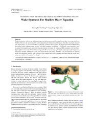
IEEE TRANSACTIONS ON COMPUTERS, MANUSCRIPT ID XXXX 10any R i that Q ∈ R i , R i ∩P ≠ ∅, which means R i ’s OB ∈P’s OB. By induction, P’s OB contains all the rules that Qmatch in X.Lemma 4.2: Given an XACML policy (or policy set) Xwith combining algorithm A, where A ∈ {Permit-Overrides,Deny-Overrides}, for any single-valued request Q, usingOB(Q) to denote the origin block of the first rule that Qmatches in AllMatch2First-Match(X,A), the winning decisionof OB(Q) is the same decision that X makes for Q.Proof: We first prove Lemma 4.2 for the base case, whereeach X i is an XACML rule. Let 〈R 1 ,···,R n 〉 denote X,where each R i is a rule. According to Lemma 4.1, OB(Q)consists of all the rules that Q matches in X. According tothe AllMatch2FirstMatch algorithm, the winning decision ofOB(Q) is determined by the combining algorithm A. Thus,the winning decision for OB(Q) is the same that X makesfor Q.We next prove Lemma 4.2 for the case where each X iis a policy or policy set and X i ′ is the equivalent sequenceof the first-match rules. In other words, for each X i , weassume that for any request Q, the origin block of the firstrule that Q matches in X i ′ consists of all the rules that Qmatches in X i . Let 〈y 1 ,···,y m 〉 be the generated rules fromthe partial PDD, which is constructed from 〈X 1,···,X ′ n〉. ′ Forany request Q, there exists at most one y i in 〈y 1 ,···,y m 〉 thatQ matches. Suppose Q matches y i , then OB(Q) is the originblock of y i . According to the AllMatch2FirstMatch algorithm,we classify OB(Q)’s origin blocks based on their sourcesand combine the OB(Q)’s origin blocks with the smallestsources in each group, because each X i ′ follows the firstmatchsemantics. After grouping, for each X i ′ , there is atmost one origin block in OB(Q) whose source is i. Thus,the winning decision of OB(Q), which is computed based onX’s combining algorithm, is the same decision that X makesfor Q.Theorem 4.3: Given an XACML policy X and its normalizedversion Y , for any single-valued request Q, X and Yhave the same decision for Q.Proof: Let A be X’s combining algorithm. If A isFirst-Applicable or Only-One-Applicable, the correctness ofTheorem 4.3 follows directly from the first-match semantics.If A is Permit-Overrides or Deny-Overrides, the correctnessof Theorem 4.3 follows from Lemma 4.2.Theorem 4.4: Given an XACML policy X and its normalizedversion Y , for any multi-valued requestQ, X and Y havethe same decision for Q.Proof: Let Q 1 ,···,Q k be the resulting single-valuedrequests decomposed from Q. If X’s combining algorithmis Only-One-Applicable, Permit-Overrides or Deny-Overrides,according to Lemma 4.1, the OB of the first rule that Q imatches in Y consists of all the rules that Q i matches inX. Thus, ∪ k i=1 O(Q i) consists of all the rules in X that Qmatches. Therefore, the decision resolved by the structure treeof X for all the rules that Q matches in X is the decisionthat X makes for Q. If X’s combining algorithm is First-Applicable, the XACML policy normalization algorithm onlycomputes the first rule that each Q i matches in X. This isequivalent to compute all the rules that Q i matches in X.V. THE POLICY EVALUATION ENGINEAfter converting an XACML policy to a semantically equivalentsequence of range rules, we need an efficient scheme tosearch the decision for a given request using the sequenceof range rules. In this section, we describe two schemesfor efficiently processing single-valued requests, namely thedecision diagram scheme, and the forwarding table scheme.We further discuss methods for choosing the appropriatescheme in real applications.A. The Decision Diagram SchemeThe decision diagram scheme uses the policy decisiondiagram converted from a sequence of range rules to improvethe efficiency of the decision searching operation. Constructinga PDD from a sequence of first-match rules is similar tothe algorithm for constructing a PDD from a sequence ofall-match rules. Fig. 9 shows the PDD constructed from〈r 1 ,r 2 ,r 3 ,r 4 ,r 5 ,r 6 ,r 7 〉 in Fig. 8.[0, 0]AR[0, 0] [1, 1]S[0, 0] [2, 3][1, 1][1, 1] [0, 0]A[0, 1][0, 0]AR[1, 1]AR[0, 1]A[1, 1] [0, 1][0, 1][R 1 ] d [R -1 ] na [R 3 ] p [[R 1 ] d , [R 2 ] p ] d [R 2 ] p [R 2 ] p [R 2 ] pFig. 9: The PDD constructed from the range rules in Fig. 8The algorithm for processing a single-valued request Qconsists of two steps. First, we numericalize the request usingthe same numericalization table in converting the XACMLpolicy to range rules. For example, a request (Professor, Grade,Change) will be numericalized as a tuple of three integers (2,0, 0). Second, we search for the decision of the numericalizedrequest on the constructed PDD. Note that every terminal nodein a PDD is labeled with an origin block.To speed up decision searching, for each nonterminal nodev with k outgoing edges e 1 ,···,e k , we sort the ranges inI(e 1 ) ∪ ··· ∪ I(e g ), i.e., all the ranges that appear on theoutgoing edges of v, in an increasing (or decreasing) order. Inthe sorted list, each range I, assuming I ∈ I(e j ), is associatedwith a pointer that points to the target node that e j points to.This allows us to perform a binary search at each nonterminalnode. 1) Complexity Analysis: Space Complexity: Suppose thesequence of range rules generated from an XACML policyis 〈r 1 ,r 2 ,···,r n 〉, where each rule r i is represented asF 1 ∈ S1 i ∧ F 2 ∈ S2 i ∧ ··· ∧ F z ∈ Sz i → 〈dec〉. For eachfield F j (1 ≤ j ≤ z) , Sj i has two end points, namelythe minimum and maximum value of the range Sj i. Thus,there are at most 2n points in the domain of F i . The totalnumber of intervals separated by the 2n points is thereforeat most 2n − 1, which means that the number of outgoingedges of a node labeled F i is at most 2n − 1. Note thatthe number of outgoing edges of a node labeled F i cannotexceed|D(F i )|. Thus, the number of outgoing edges of a nodelabeled F i is at most min(|D(F i )|,2n−1). Therefore, theworst case space complexity of the decision diagram schemeis O( ∏ zi=1 min(|D(F i)|,2n−1)).Time Complexity: As we discussed above, the total numberof intervals on the outgoing edges of a node labeled F i isat most min(|D(F i )|,2n−1). Hereby, the time complexityfor processing a single-valued request based on the PDD isO( ∑ zi=1 log(min(2n−1,|D(F i)|))).
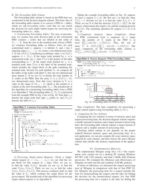
()IEEE TRANSACTIONS ON COMPUTERS, MANUSCRIPT ID XXXX 11B. The Forwarding Table SchemeThe forwarding table scheme is based on the PDD that wasconstructed in the decision diagram scheme. The basic idea ofthe forwarding table scheme is to convert a PDD to z tables,which we call forwarding tables, such that we can searchthe decision for each single-valued request by traversing theforwarding tables in z steps.1) Constructing Forwarding Tables: For ease of presentation,we assume that each decision path in the constructedPDD contains z nodes that are labeled in the order ofF 1 ,···,F z from the root to the terminal node. Given a PDD,we construct forwarding tables as follows. First, for eachnonterminal node v, suppose v is labeled F i and v has koutgoing edges e 1 ,···,e k , we create a one-dimensional arrayT of size |D(F i )|. Considering an arbitrary value m in D(F i ),suppose m ∈ I(e j ). If the target node pointed by e j is anonterminal node, say v ′ , then T[m] is the pointer of the tablecorresponding to v ′ . If the target node pointed by e j is aterminal node, then T[m] is the label of the terminal node,which includes the origin block of the path containing theterminal node. Second, for each attribute F i , we compose allthe tables of the nodes with label F i into one two-dimensionalarray named T i . If we use M i to denote the total number ofF i nodes in the PDD, then the array T i is a |D(F i )| × M itwo dimensional array. Note that every element in T i is avalue in the range [0,M i+1 − 1], which is the pointer to acolumn in the next forwarding table T i+1 . The pseudocode ofthe algorithm for constructing forwarding tables from a PDDis in Algorithm 5. The forwarding tablesT 1 ,T 2 ,T 3 constructedfrom the example PDD in Fig. 9 are in Fig. 10. Note that e g .tdenotes the target node that edge e g points to, and F(e g .t)denotes the label of e g .t.Algorithm 5: Construct Forwarding TablesInput: A PDD.Output: Forwarding tables T 1,···,T z.1 put the root into queue Q;2 while Q ≠ ∅ do3 sum := 0;4 for j := 0 to sizeof(Q) − 1 do5remove node v from Q;6/*Suppose F(v) is F h and v has k outgoing edgese 0,e 1,···,e k−1 .*/7if F h ≠ F z then8for i := 0 to |D(F i)| − 1 do9if i ∈ I(e g) then T h [i,j] := sum + g;10111213141516sum := sum + k;for g := 0 to k − 1 do put e g.t in Q;elsefor i := 0 to |D(F i)| − 1 dofor g := 0 to k − 1 doif i ∈ I(e g) then T z[i,j] := F(e g.t);return T 1,···,T z;2) Processing Single-valued Requests: Given a singlevaluedrequest Q = (m 1 ,···, m z ), we can find the originblock for this request in z steps. First, we use m 1to find the value T 1 [m 1 ]. Second, we use m 2 to find thevalue T 2 [m 2 ,T 1 [m 1 ]]. Third, we use m 3 to find the valueT 3 [m 3 ,T 2 [m 2 ,T 1 [m 1 ]]]. This process continues until we findthe value in T z , which contains the origin block for thegiven request. The pseudocode of the algorithm for processingsingle-valued requests is in Algorithm 6.Taking the example forwarding tables in Fig. 10, supposewe have a request (1,1,0). We first use 1 to find the valueT 1 [1] = 1. Second, we use 1 to find the value T 2 [1,1] = 3.Third, we use 0 to find the decision T 3 [0,3] = [R 2 ] p for therequest, which means the origin isR 2 and the winning decisionis permit. The searching operation for request (1,1,0) is inFig. 10.3) Complexity Analysis: Space Complexity: Giventhe PDD constructed from a sequence of n rangerules,∏the number of F i nodes in the PDD is ati−1mostj=1 min(2n−1,|D(F j)|). Thus, the size ofarray T i is |D(F i )| ∏ i−1j=1min(2n−1,|D(F j )|). Thespace complexity of the forwarding table scheme isO( ∑ zi=1 (|D(F i)| ∏ i−1j=1 min(2n−1,|D(F j)|))).Algorithm 6: Process Requests With Forwarding TablesInput: (1) A single-valued request (m 1,···,m z).(2) Forwarding tables T 1,···,T z.Output: The origin block for the single-valued request.1 j := 0;2 for i := 1 to z do3 if i = z then return T z[m z,j];4 else if i = 1 then j := T 1[m 1];5 else j := T i[m i,j];T 2A request T 1 0 01 1 11 2 20 1 203 20 0 2 41 1 3 4T 30 1 2 3 40 [R 1 ] d [R 3 ] p [ [R 1 ] d , [R 2 ] p ] d [R 2 ] p [R 2 ] p1 [R -1 ] na [R 3 ] p [R 2 ] p [R 2 ] p [R 2 ] pFig. 10: Forwarding tables for PDD in Fig. 9Time Complexity: The time complexity for processing asingle-valued request using forwarding tables is O(z).C. Comparing the Two SchemesComparing the two schemes in terms of memory space andrequest processing time, the decision diagram scheme requiresa smaller amount of memory and a larger amount of processingtime; the forwarding table scheme requires a larger amount ofmemory and a smaller amount of processing time.Choosing which scheme to use depends on the propertradeoff between memory space and processing time. In areal application, we can pre-compute the exact memory spacerequired by each scheme, and then choose the more efficientscheme that satisfies the memory requirement of the application.VI. EXPERIMENTAL RESULTSWe implemented XEngine using Java 1.6.3. Our experimentswere carried out on a desktop PC running WindowsXP SP2 with 3.5G memory and dual 3.4GHz Intel Pentiumprocessors. We evaluated the efficiency and effectiveness ofXEngine on both real-life and synthetic XACML policies.In terms of efficiency, we measured the request processingtime of XEngine in comparison with that of Sun PDP [2].For XEngine, the processing time for a request includes thetime for numericalizing the request and the time for findingthe decision for the numericalized request. For Sun PDP,the processing time for a request is the time for finding the
Page 1 and 2: IEEE TRANSACTIONS ON COMPUTERS, MAN
Page 14: IEEE TRANSACTIONS ON COMPUTERS, MAN

Designing Fast and Scalable XACML Policy Evaluation Engines

Create successful ePaper yourself

Delete template?

Save as template?