Removing the Stiffness from Interfacial Flows with Surface Tension

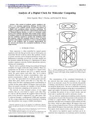
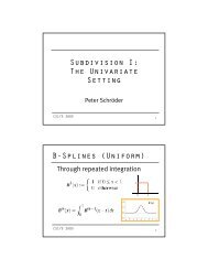
FLOWS WITH SURFACE TENSION 315lower order terms in the evolution. There is also an equationanalogous to Eq. (8) for L. Such a reformulation of fluidinterface evolution, as in Eq. (11 ), is a "small scale decomposition."It is within the small scale decomposition thatimplicit integration or linear propagator methods can beapplied to a high order linear term. With periodic boundaryconditions, these methods are explicit in Fourier space andhave no high-order time step constraint. The time-steppingmethods are coupled to spectrally accurate spatial discretizations.Small scale decompositions are given also formore general Hele-Shaw flows and for interface flows underthe Euler equations.An example of what is possible with these methods is seenin Fig. 1, which shows the simulation of a gas bubbleexpanding into a Hele-Shaw fluid (see [ 15, 16]) over longtimes. From the competition of surface tension with the fluidpumping, this simulation shows the development oframification through successive tip-splitting events and thecompetition between adjacent fingers. This simulation isalso spectrally accurate in space and uses a second-order intime linear propagator method for integrating the smallscaledecomposition. There are no high-order time stepconstraints. The fluid velocity is calculated using the fastmultipole method [23], and GMRES [42] is used to solvethe integral equation that arises from having a viscosity con-" trast [22]. The operation count is O(N) at each time-step,where N is the number of points describing the boundary.Here N= 4096, S = 0.001, and At = 0.001. The time step is103 times larger than that used by Dai and Shelley [ 16] incomputations of a similar flow using an explicit method15with a lesser number of points, and the interface here hasdeveloped far more structure.The organization of the paper is as follows. In Section 2,boundary integral formulations are given for the motion offluid interfaces under surface tension in both Hele-Shawand two-dimensional Euler flows. The interface is interpretedas a vortex sheet whose normal velocity is determinedby the Birkhoff-Rott integral. Its vortex sheetstrength is determined by the equations of motion andboundary conditions. In Section 3, the source of stiffness inthese problems is discussed and motivated by thegeneralized linear stability analysis of Beale, Hou, andLowengrub [10-12]. In Section4, the Birkhoff-Rottintegral is carefully examined. It is shown that this integral,asymptotically at small scales, becomes a Hilbert transformof the sheet strength over a flat interface, with a variableprefactor. In Section 5, the description of the interface isreformulated in terms of 0 and L. This step makes thevariable coefficient depend only upon time, and at smallscales, the leading order terms are only nonlocal through aHilbert transform. This leads to small scale decompositionsfor the evolution problems. In Section 6, numerical methodsare discussed. This includes second-order integrationmethods that exploit the small scale decomposition toremove the high-order stiffness, generalizations to higherorder time discretizations, as well as other related numericalissues such as spectrally accurate spatial discretizations. InSection 7 the results of numerical simulations using thesemethods are presented. These results include the motionof Hele-Shaw interfaces moving under the competinginfluences of gravity and surface tension, in addition to theexpanding gas bubble. The roll-up and collision of vortexsheets with surface tension in an Euler flow is also given.Concluding remarks are given in Section 8.10-5-10-15-1I I I I I-10 -5 0 5 10 15Time =0 to 45FIG. 1.An expanding Hele-Shaw bubble.2. THE FORMULATIONIn this section, boundary integral formulations are givenfor two illustrative incompressible flows. The first describesthe motion of an interface separating two Hele-Shaw fluidsof differing densities and viscosities. The second describesthe motion of a vortex sheet in a two-dimensional, inviscidfluid. As the concept of a vortex sheet arises also in theHele-Shaw case, this second case is referred to as an inertialvortex sheet.Consider an incompressible and irrotational velocity fieldin two dimensions given in terms of a velocity potential:(u,v)=V~. Suppose that ~b has a jump across aparametrized interface F= (x(~), y(0~)), but that its normalderivative is continuous (see Fig. 2). This implies that thevelocity has a tangential discontinuity across F while thecomponent normal to F is continuous (i.e., the kinematicboundary condition is satisfied). Such an interface is called

316 HOU, LOWENGRUB, AND SHELLEYP$-~pa,/z2FIG. 2. A schematic showing F, the interface separating twoHele-Shaw fluids.a vortex sheet (see [43 ] ). The velocity away from the interfacehas the integral representation(u(x, y), v(x, Y))1 f (--(y-y(og)),x-x(og)) , ,J ~(~') (x - x(¢)) ~ + (y- y(¢))= ao~+ V(x, y, t), (12)where (x,y)¢(x(oQ, y(ct)). The velocity V accounts forother contributions to the motion not given by the integralterm. V is assumed smooth, at least across F, and can arisefor many reasons, such as to satisfy far-field boundary conditionsor to account for other interfaces. 7 is called the(unnormalized) vortex sheet strength and measures thevelocity difference across F. It is given by~(~)=s,((u,, v~)-(u2, v2))l~.s.This representation is well known; see [6 and 51, 27] forsome applications to inertial and Hele-Shaw flows, respectively.While there is a discontinuity in the tangential componentof the velocity at F, the normal component, U(00, iscontinuous and is given by (12) aswhere1w(~) =~ P.V. f ~(~')U(~)=W(~).nviscosities, and densities. For simplicity, F is assumedperiodic in the x-direction. The fluid below F is labeledfluid 1 and that above is labeled fluid 2, and likewise fortheir respective viscosities, etc. The density and viscosity areassumed to be constant above and below F, but they candiffer across F. The velocity in each fluid is given by Darcy'slaw, together with the incompressibility constraint:b 2oj= (uj, vj) = 12ktjV(ps-psgy), V.uj= O. (16)Here b is the gap width of the Hele-Shaw cell, pj is theviscosity, pj is the pressure, Ps is the density, and gy is thegravitational potential. The boundary conditions we takeare(i) [U]r'n =0, the kinematicboundary condition (17)(ii) [ P ] r = zK, the Laplace-Youngcondition (18)(iii) uj(x,y)-~O as lyl---' ~, (19)where [ f ] r = fl - f2 and fl, f2 are the limiting values from(13) below and above the interface, respectively. In addition, x isdefined as in Eq. (1) so that a circle has positive curvature.Condition (i) requires that F moves with the fluids on eitherside. Condition (ii) relates the pressure jump across F to theinterfacial curvature x, where z is the surface tension.Condition (iii) specifies that the fluid is at rest far from theinterface.That the velocity field has the form given in (12) withV = 0 follows from Darcy's law (16), which implies that the(14) flow is irrotational, the incompressibility constraint, andfrom the boundary conditions (i) and (iii). An equation for7 follows from these, together with the Laplace-Young condition(ii); see [51 or 16] for details. In nondimensionalvariables, 7 satisfies(- (y(0Q- y(0()), x(0Q - x(ct'))x (x(~) -x(~')) 2 + (y(~) - y(~,)12d~'+V (15)and P.V. denotes the principal value integral. This integralis called the Birkhoff-Rott integral. This representation canbe given for closed or open interfaces and for situations withmultiple fluids and interfaces. For Hele-Shaw and Eulerflows, our two main examples, the full formulations nowfollow.2.1. Hele-Shaw FlowsConsider an interface F, as shown in Fig. 2, whichseparates two Hele-Shaw fluids of differing, but uniform,7 = -2Aus~W. ~ + Sx~- Rye. (20)is the Atwood ratio of theviscosities, S is the nondimensional surface tension, and R isa signed measure of density stratification (Pl

FLOWS WITH SURFACE TENSION 317Again, the shape of the interface is determined solely by thenormal velocity, and a choice of tangential velocity onlymodifies the frame of the parametrization. Accordingly, themotion of F is given byX,(~, t) = (x,, y,) = Un + Ts. (21)Once T is specified, Eqs. (20) and (21) determine the entireflow through the motion of F. The usual choice of frame,T = W. s, is called the Lagrangian frame and corresponds tochoosing T to be the average of the limiting tangential fluidvelocities from above and below F.Remarks. (1) Hele-Shaw flow can also be interpretedas two-dimensional porous media flow. There is also acorrespondence of the Hele-Shaw flow to the Ostwaldripening problem, a quasi-stationary appoximation to diffusion.See [52], for example.(2) Only the simplest, classical dynamic boundary conditionfor Hele-Shaw flows have been considered here.More physically realistic boundary conditions have beenderived in [ 40 ].2.2. Inertial Vortex SheetsThe formulation of the motion of an interface, F,separating inviscid, incompressible, and irrotational fluids,is similiar to that for the Hele-Shaw case. As before, thedensity is assumed to be constant on each side of F. Here,the velocity on either side of Fis evolved by Euler's equationujt+(uj.V)uj=-lv(&+pjgy), V. uj= O. (22)&where Ap=(pl--P2)/(pl+P2 ) is the Atwood ratio ofdensities and S= 2z/(pl + P2) is a rescaled surface tensionparameter (see [6, 45]). In contrast to Hele-Shaw flows,the vortex sheet strength y is an independent dynamicvariable. This is because the motion is governed by inertialforces (Euler's equation) rather than by viscous forces(Darcy's law). And now, Eq. (27) is a Fredholm integral ofthe second kind for y, due to the presence of ~)t in W,. Thekernel of the equation is the same as that in the Hele-Shawintegral equation with A, replaced by Ap. Finally, the meanof 7 is preserved by Eq. (27) and must be chosen to be 2 Vo,initially, to guarantee that condition (iii) is satisfied.3. STIFFNESS AND LINEAR THEORYNumerical stiffness arises through the presence of highorderterms (i.e., many spatial derivatives) in the evolution.The role of surface tension in producing numerical stiffnessis illustrated by considering first the linearized equations ofmotion about the flat equilibrium. That is, considerx(ct, t) = ~ + e~(~, t) and y(ct, t) = eq(ct, t), with e ~ 1. This issufficient for Hele-Shaw flows as ~ is a dependent variable.For inertial vortex sheets, this is suppliemented by 7(~, t) =So + ee~(0~, t), where 7o is a constant. For definiteness, theLagrangian frame T= W. s is taken, and for simplicity,A, = A s = 0 for both the Hele-Shaw and inertial flows.The linearized Hele-Shaw equations of motion arewhere ~ is the Hilbert transform,~t=0 (28)qt=½Jf[Sq=~-Rr/~], (29)There are now the boundary conditions:(i) [U]r-n=0 (23)(ii) [P]r=rX (24)(iii) nj(x,y)--*(+_Vo, O) as y~ _+~. (25)Since the fluid is irrotational and incompressible, condition(i) again guarantees a vortex sheet representation of thesolution, again with V = 0. Using the representation (12) ofthe velocity, Euler's equation at the interface, and theLaplace-Young condition, the equations of motion for theinterface areX t = Un + Ts7,- O~((T- W. s) 7/s~)= - 2AAs,Wt. s + 1~,(~/s~)2 + gy,- (T-W-s) W~ .s/s~) + Sx~,W[f](ct)1 f+~ f(a') do~'. (30)n -oo 0~--0~'is a skew-symmetric linear operator, is diagonalized bythe Fourier transform, and satisfies~[e ikx] = - i sgn(k) e ikx, af[1] =0. (31)Consequently, the linear growth rate for the amplitudeperturbation t/isak= --½(S Ikl3 +R Ikt). (32)Therefore, if R < 0, there is a band of unstable modes near(26) k = 0. This is a Saffman-Tayl0r type instability, driven bythe unstable density stratification. At higher wavenumbers,this instability is cut off by the surface tension term whichacts as third-order diffusion. Thus, in linearized Hele-Shaw(27) flows, surface tension is a dissipative regularization.

318 HOU, LOWENGRUB, AND SHELLEYThe source of stiffness is made clear by the linear motion.The stability constraint for an explicit time integrationmethod applied to Eq. (29) has the form~It ff[rl~] + S1 )ffEq=~]. (34)S~ S aA "frozen coefficient" analysis of Eq. (34) reveals the stricterstability constraint~It < C. (g=h)3/S, (35)where g,=min, s,. Therefore, the stability constraint isdetermined by the minimum grid spacing in arclength,which is strongly time dependent. Our experience is that theLagrangian motion of the points can lead to "pointclustering" and hence to very stiff systems, even for flows inwhich the interface is smooth and the surface tension issmall.For inertial vortex sheets, the growth rate for perturbationsabout the flat equilibrium is given byS~2 = V~k2_~ ikl 3. (36)Again, the surface tension controls a high wave-numberinstability. The instability here is the Kelvin-Helmholtzinstability and it is due to the shearing motion across theinterface. As can be seen from the growth rate, the surfacetension is a dispersive regularization in contrast to theHele-Shaw case where it is dissipative. Again, by linearizingaround the time dependent inertial vortex sheet F=(x(0~, t), y(~, t)) with strength 7(~, t), Beale et al. [ 10, 12]find the dominant behavior for r/, again the normal componentof the perturbation, to be),2 Stltt= --~S J~O[t/~ct~t]'a'=4 ?/~t"3I- ~-~-3 2s= (37)The perturbation in y is eliminated, to leading order, byusing two time derivatives on ~/. A frozen coefficient analysisleads to the dynamic stability constraintWhile the time step constraint (38) is less restrictive thanthat for Hele-Shaw flows, our experience is that pointclustering, through the Lagrangian point motion, still leadsto prohibitively stiff systems.4. THE SMALL SCALE BEHAVIOR OF UThe stiffness of an explicit method occurs because theevolution at small length scales is controlled by a high orderterm introduced by the curvature. The normal velocity Ufrom the Birkhoff-Rott integral contains the physically relevantpart of the velocity field, and the curvature appears init through the vortex sheet strength. In this section, thesmall scale behavior of U is analyzed and precisely determinedin terms of the vortex sheet strength.First, the normal velocity U is given in a convenient form.Let the complex position of the interface be given byz(e, t) = x(e, t) + iy(~, t). Then, the normal velocity is givenbyU(o~,t)=_llm{Z ~ +oo y(o~',t) }P.v. f tl .(39)This quantity is clearly related to the Hilbert transform ofthe vortex sheet strength 7 over the curved interface F. Ouroriginal intuition was that the small-scale behavior of thisexpression could be found by simply retaining one term inthe expansion of the denominator in the Birkhoff-Rottintegral to yield a Hilbert transform over a flat interface,z = ~t, with a variable coefficient prefactor. This intuition isset rigorously in the following way. The kernel in theBirkhoff-Rott integral is rewritten as1 1mz(o~,t)-z(og, t) z,.(o~-o~')[ 1+ z(oq t)- z(og, t)(40)Note that the bracketed term has a removable singularity at= e', provided that z is a smooth function ofcq the interfacedoes not self-intersect, and s~ > 0. The Birkhoff-Rottintegral can then be rewritten asf+~ 7(0~', t)P.V. -~ z(cq t) -z(~', t) d0(n ~ff[7]=_ +f+~Z~ oo7(~',t)g(ot, o~',t) d o~',(41)At < C. (gah)3/2/S. (38) where g is the term in the brackets of Eq. (40). Thus, the

FLOWS WITH SURFACE TENSION 319integral term containing g is a smoothing operator on y.This proves the following result.TrmOREM 1 (Small scale behavior of U). Suppose thatthe coordinates ofF, (x(oc, t), y(ct, t)), are real analytic functionsof oc for t O. ThenU(0c, t)=~s ~[y](0c , t)+E[y](oq t) (42)for t

320 HOU, LOWENGRUB, AND SHELLEY8~s=xn and 8~n= -xs, together with O~=x and O/8s=(1/s~)(8/OoO, it is easy to see that s~ and 0 satisfys~t=T~--O~U (51)O, =--1 u~+T o~. (52)S~ S~Given s~ and 0, the position (x(a, t), y(0c, t)) is reconstructedup to a translation by direct integration of Eq. (49). In manyproblems, the motion is translation invariant and thus thislost constant is irrelevant. However, a single point on theinterface can be evolved to provide the constant of integration.The velocities U and T can then be constructed and s~and 0 updated through Eqs. (51) and (52).5.1. The Equations of Motion ReposedUsing this formulation, the general small scale decompositionis given for Hele-Shaw and inertial flows. Thedominant small scale behavior is assumed to come from theU~ term in the 0 equation and the curvature term in the yequation. U~ explicitly contains the curvature in theHele-Shaw case and the vortex sheet strength in the inertialvortex sheet case. The evolution of s~ will be recast in termsof L in the next section.(A)Small scale decomposition: Hele-Shaw flow. For theHele-Shaw case, using that tc = O~/s~ and recalling Eqs. (45)and (47), Eq. (52) becomes=s2(±0, 2s ,s+ ~U~ 2s~\s~* ~ ~ ~ +lO~Ts= (53)O~-SI (I~I~],),+N(cc't"2s, (54,where N is defined as the remaining terms, on the right-handside of Eq. (53), not included in the first term. By extractingthe dominant term, the Hele-Shaw evolution is now in aform that reveals clearly the dominating behavior at smallscales. But most importantly, if s, is considered to be given,the dominant small scale term is linear in the tangentangle 0, but nonlocal by virtue of the Hilbert transform andvariable coefficient by the presence of s~.(B) Small scale decomposition: Inertial vortex sheets.Analogously, Eqs. (45) and (48) are used to give the 0 andy evolution for an inertial vortex sheet, in a way that displaysthe small scale dominating terms,ll(1 ) +P, (55)X~ = \s~l~+Q.ct(56)Again, P and Q represent the remainder terms. Assuming,as before, that s, is given, the dominant small scale terms arelinear in 0 and 7, nonlocal, and also variable coefficient.As was the case for curve shortening ( U = x), the leadingorder terms in both cases (A) and (B) simplify considerablyif s~ is independent of co. Again, this is enforced by a choicefor T, the tangential velocity. We do remark, though, that insome situations it may be preferable to use other choicesof T. Other choices may prove to be useful to resolve regionsof high curvature or to naturally handle anisotropic surfaceenergies. If that is the case, the general small scale decomposition,given above, may still be useful for implicitintegration methods since the leading order terms are linearin0 (and X). Additional reference frames are given inAppendix 2 and are currently under study.5.2. The 0 - L FormulationThe general expression for T is now given so that s~ isindependent of ~ in its evolution; s= will then depend onlyupon t, and the PDE (51) for s~ reduces to an ODE.Moreover, the dominant terms at small scales in Eq. (54) forHele-Shaw and Eqs. (55) and (56) for inertial vortex sheets,become constant coefficient in space.As in the Introduction, s~ is required to be everywhereequal to its mean, that iss~(oq t) = sw(~', t) d~' = L(t), (57)where L is the length of the interface. By differentiatingEq. (57) with respect to t and using Eq. (51), Tis found tobeT(c~,t)=T(O,t)+ O~,Vdoc-~ O~,Vdoc', (58)fowhich expresses T entirely in terms of 0 and U. The spatialconstant T(0, t) just gives an overall temporal shift in frame.For simplicity, it will be taken to be 0, although in principle,it could be evolved as well. Thus, if s, is initially uniformin ~, then the choice for T in Eq. (58) will maintain thatconstraint in time. An expression for L, is found directly byusing Eqs. (51), (57), and (58). The evolution of the interfaceis now given in terms of L and 0 by/, 2~L t = -| 0~, UdoC (59)ao0,= T (60)Given U, Eqs. (58), (59), and (60) are a complete formulationof the evolution problem. We note that this choice offrame through T is actually a special case of other, moregeneral choices of frames. See Appendix 2.

FLOWS WITH SURFACE TENSION 321The small scale decompositions for Hele-Shaw and inertialvortex sheet flows in the 0-L formulation are nowgiven:(A) Small scale decomposition: Hele-Shaw flow. In the0- L formulation, Eq. (55) simplifies tos(2"/3O'=2\Lj+ut t(61)Here, N is that inferred from Eq. (54) with the choice of Tin Eq. (58). Equation (61 ) is posed, together with Eq. (59),the ODE for evolving L, and is a complete specification ofthe interfacial problem, with the highest order, linearbehavior prominently displayed. This term is nowdiagonalizable by the Fourier transform, and soO,(k) = - ~ Ikl 30(k) + ~(k). (62)Implicit time integration methods, such as Crank-Nicholson differencing, or linear propagator methods, cannow be easily applied.(B) Small scale decomposition: lnertial vortex sheets.Analogously, for the inertial vortex sheet, the equations ink'-space areOt(k)= ~ lkl (~)2 ~(k) + P(k), (63)~,(k) = -Sk 2 ~ O(k) + O(k). (64)LHere, P and Q are those inferred by in Eqs. (55) and (56),with the choice of T in Eq. (58). The diagonalization of theleading order, linear system is trivial. And again, these equationsmust be posed together with Eq. (59).6. NUMERICAL METHODSIn this section, discrete methods are discussed for computingthe motion of inertial vortex sheets and Hele-Shawinterfaces. We begin by considering two types of timeintegration methods. Both methods use the 0-L smallscale decomposition in a crucial way. The first uses anintegrating factor to remove the leading order term andgives an explicit time discretization under the Fourier transform.This is the linear propagator method. The second is animplicit Crank-Nicholson discretization of the leadingorder term, which also gives an explicit method under theFourier transform. Spatial discretizations are chosen to bespectrally accurate.Assume for now that space is continuous. We begin bydiscussing the time integration of the length L. Its ordinarydifferential equation (59) can be discretized with an explicitmethod. In the calculations presented here, the secondorderAdams-Bashforth method is used,L .+1 =L.+_~(3M._M.-1), (65)where the superscript denotes the time level and M is givenbyM= -- f0 TM 0~, Ud~'. (66)As this is an explicit method, L can be updated before either0 or T. The 0 (and V) discretizations will require thisupdated L.6.1. Hele--Shaw Time DiscretizationsThe Linear Propagator MethodLinear propagator methods factor out the leading orderlinear term prior to discretization. They usually providestable, even high-order, methods for integrating diffusiveproblems. Linear propagator methods apply also to dispersiveproblems, but must be used more carefully. Thesemethods have the property that in the absence of nonlinearityand variable coefficients, the discrete solution givesthe exact solution to the constant coefficient linear problem.That is, the linear modes are propagated exactly. The firstuse of such a method (of which the authors are aware) isRogallo [41] in simulations of the Navier-Stokes equations,although it has been rediscovered and used by severalresearchers in different contexts.For Hele-Shaw, we rewrite Eq. (62) aswhereOt ~b(k' t)=exp (2zclkl) 3 ~t dt' ) ~(k, t), (67)Jo L3(t')]S ' dt' ) O(k, t)~k(k, t)= exp (2x Ikl)3 ~0 Z3(t')J (68)Equation (67) follows from Eq. (62) by finding an integratingfactor to incorporate the linear term into the timederivative. It is now Eq. (67) that is discretized using thesecond-order Adams-Bashforth method. In terms of 0, theresult iszttOn* l(k)=ek(tn, tn+ l) i~n(k) +-~ (3ek( tn, t~+l) ~n(k)--ek(t~_~, tn+ 1)/~"-l(k)), (69)

322 HOU, LOWENGRUB, AND SHELLEYwhere t. = n At, andand soS t2 dt' "]ek(tl, tz) = exp -- ~ (2zr ]kl) 3 ft, za(t')J" (70)The use of "linear propagator" is now clear; 0 at the n thtime step is propagated forward to the (n + 1 )th timestep atthe exact exponential rate associated with the linear term. IfN-0, this yields the exact solution to the linear problem.Of course, the factor e(tl, t2) still has a continuous timedependence. We retain second order by replacing theintegrals with their trapezoidal rule approximations, i.e.,1ek(t., tn+l)=exp (-S~t(21r lkl)3[(~ ~ (Ln~- 1)3])SAtek(tn_l, tn+l)=exp -----~-(2/l:lkl) 3 (71)- 1X _2( Ln _ 1 ) 3Thus, in the numerical scheme, 0 is propagated by a secondorderapproximation of the exact exponential rate. Recallthat L" +1 is computed explicitly by Eq. (65).Remarks. 1. Near equilibrium, the second-order linearpropagator method is unconditionally stable. That is, werequire only d t ~< C(S) independently of the wavenumber k.More generally, however, there may be a CFL conditionarising from the transport term hidden in N (see Eqs. (53)and (54)). This term is not seen in the near equilibriumanalysis. The long time simulations are always performedwith a CFL condition in mind. The exponential dampingfactors also tend to suppress instabilities such as thosearising from aliasing errors or underresolution. It has alsobeen observed that, in the presence of singular behavior ofthe interface, this method tends to oversmooth the solution[ 19]. This difficulty is overcome by reducing the timestep. We believe that it may also be ameliorated by usinghigher order time discretizations. If the solution is smooth,then this difficulty is not noticeable.2. An advantage of a linear propagator method is thatit is easy to derive higher order time discretizations. This isclear if there is no time-dependence in the coefficient of thelinear term. On the other hand, if there is time dependence(as is the case here), then a time integral appears in theintegrating factor (see Eq. (68)). An explicit quadrature ofthis integral is avoided by introducing a new independentvariable corresponding exactly to the integral. LetI= I[L](t) be given byI(t)= fo1dt'L3(t,) (72)1I t = L--- 3, I(0) = 0. (73)Then, we supplement the original system (59) and (67) andsolveL, = M[L, I, ~k](t) (74)1I, =~--~ (75)~k, = eZ(S/2)~z~lkl)3b~[ L, L ~b](k, t). (76)It is now straightforward to discretize this system to highorder. Fourth-order Runge-Kutta is currently beingimplemented.Crank-Nicholson DiscretizationAnother stable scheme is obtained by using theCrank-Nicholson discretization on the leading order stiffterm and leapfrog on the nonlinearity. This gives thesecond-order integrationO°+l(k)--O° l(k)2At+ A?"(k). (77)Since L n+l, L n, and L n-1 are known, Eq. (77) gives anexplicit expression for O n + l(k).Remarks. I. A near equilibrium analysis shows thatthis method is unconditionally stable. Again, there may bea CFL condition from the transport term. Our computationsconfirm stability for short times, but they also indicatethat for long times and, in the fully nonlinear regime, thatthe Crank-Nicholson method is susceptible to an aliasinginstability. The time of onset of this instability increases asthe spatial resolution is increased. However, we find that wecan control this instability and retain accuracy, even overlong times, by the application of a high-order Fourier filter(25 th order). We will discuss this further when we give thespatial discretizations and numerical results.2. The Crank-Nicholson discretization may also be usefulto compute in other frames of reference (i.e., using otherchoices of T). Of course, s~ is no longer constant in ~, butthe general small scale decompositions (54) and (55), (56)still apply. The PDE for s, is not expected to be stiff and theleading order terms in the 0 (and y) equations are still linearin 0 (and y), albeit with variable coefficients. Thus by

FLOWS WITH SURFACE TENSION 323updating s~ explicitly, a linear, but not diagonal, systemcan be obtained fer the updates of 0 (and 7). This systemcould then be solved by an iterative method such asGMRES [42].O__ (e --i x/(S/2)(2~ Ik[) 3 IO (dt'/L3/2(t'))l) 1 )0t= e-i'/(s/2)(2" Ikl) 3 ~ (dt'/L3/2(t'))~, 1(8o)6.2. Inertial Vortex Sheet Time DiscretizationsThe Crank-Nicholson DiscretizationA stable integration can be obtained by discretizingthe leading order stiff terms implicitly using the Crank-Nicholson discretization. There are two possible ways ofdoing this. In one, the Eqs. (63) and (64) are diagonalizedbefore the Crank-Nicholson discretization is used.However, we find it sufficient (and simpler) to use theCrank-Nicholson discretization directly on Eqs. (63) and(64), to give the method# n + 1 -- ~n 12At=[klf(4 \\Ln+lj2n ~2 n \{ 2~ ~2 )+l..~/Ln_l / ~,-1 +P"(k) (78)2At=1Sk: ( 2z: On+l+L~_lOn_l)+On(k)" (79)Now O"+~(k) and )3n+l(k) can be found explicitly byinverting a 2 x 2 matrix.Remarks. 1. A near equilibrium analysis shows thatthis method is unconditionally stable. Again there is thepossibility that a CFL condition must be satisfied. As in theHele-Shaw case, this method suffers from an aliasinginstability at long times in the fully nonlinear regime. Asbefore, the onset time increases with increasing resolution.And again, we find that we can control this instability andretain accuracy, even over long times, by the application ofa high-order Fourier filter (25 th order).2. The scheme resulting from diagonalizing Eqs. (63)and (64) first, and then applying Crank-Nicholson is alsounconditionally stable near equilibrium. It has not beenimplemented.3. As in the Hele-Shaw case, the Crank-Nicholson discretizationis adaptable to different choices of referenceframes.The Linear Propagator MethodA linear propagator method can also be constructed. Thisinvolves diagonalizing Eqs. (63) and (64) so as to writewhereTt(e i ~/(s/2)(2n Ikl )3 j~ (dt,/L3/2(t,))U2= e i x/(S/2)(2zc Ikl) 3 ~ (dt'/L3/2(t'))~2 '(81)V = (Vl, /)2) = ~r~--I W, W= (0, ~) (82)F--(F1,F2)--a-IF-~-IQt v, F=(/5,0) (83)with the basis matrix 0 given byg2= 2 \L/ 2 \LJ |F(2 Ikl73 s7' 2/-iL\-Z-; JThese equations can now be straightforwardly discretizedin time in an analogous manner as was done for theHele-Shaw case (see the previous section). The secondorderAdams-Bashforth method is implemented for theseequations. While it is difficult to identify analytically thestability constraint near equilibrium, it is clear that thisdiscretization is not unconditionally stable. While there iscertainly a restriction of the form At

324 HOU, LOWENGRUB, AND SHELLEYtime-stepping instability. This instability is observed in timecontinuous and space discrete schemes. It is due to thefact that lower order schemes unphysically suppress thestabilizing effects of surface tension at the highest modes.Beale et al. [ 12] show how lower order accurate schemescan be modified to be stable and convergent. However, noneof these works address the issue of the temporal stabilityconstraints, which is a central focus of the work here.We use spectrally accurate spatial discretizations. Anydifferentiation, partial integration, or Hilbert transform isfound at the mesh points by using the discrete Fourier transform(DFT). To compute the complex Lagrangian velocityof the interface (84), we use the spectrally accurate alternatepoint discretization-' --- ~ ykcot , (85)uj tVJ -- 4r~i j + k oddwhere zj-=-xj + iyj denotes the approximation to the positionof the interface at the grid point jh with h = 2zr/N, andN is the number of grid points (see [ 46, 44 ]). Similar spectrallyaccurate quadratures employing prior removal of thesingularity are given by Baker [4]. Other integrals over theperiod, such as that in Eq. (66), are evaluated to spectralaccuracy using the trapezoidal rule.Care must also be taken with spectrally accuratemethods. Although a near equilibrium, spatially discreteanalysis indicates that they are stable [7, 10, 12], thisanalysis involves only constant coefficients of perturbedquantities. Beale et al. [ 12] performed also a spatially discretelinear analysis far from equilibrium and noted that thespatial variation of coefficients leads to aliasing errors.These errors can be destabilizing if left uncontrolled, andBeale et al. describe several types of Fourier filtering thatguarantee stability and convergence. Such errors arise as aresult of the imposed periodicity on the discrete solutions inboth space and wavenumber, and the resultant instabilitieshave been well studied in the context of hyperbolic equations.See [21, 25, 32, 49], for example. Fourier filtering isoften used to remove them.Typically, if the time discrete method is not smoothing atthe highest modes, then aliasing instabilities can occur overlong times. The linear propagator method for Hele-Shawflows is inherently smoothing at the highest modes, due tothe exponential damping factors and does not sufferfrom aliasing instabilities. The other methods we havedescribed--Crank-Nicholson for Hele-Shaw flows andboth methods for inertial vortex sheets-~lo suffer fromaliasing instabilities since they are not naturally dampingat the highest modes. As is expected with an aliasinginstability, its onset time increases as the spatial resolutionis increased. Thus, in principle, the instability can becontrolled by simply increasing the spatial resolution. Thisis expensive. Instead, the instability is controlled by usingFourier filtering to damp the highest modes. In particular,the 25 th order Fourier filter/~[f](k) -- e-1°(Ikr/u)25f(k) (86)is employed. The filtering determines the overall accuracy ofthe method, and so the formal accuracy is O(h25). Certainlyan infinite-order filter could have been used, but we did notdo so. In addition, as high derivatives are computed in thecode, Krasny filtering [31 ] (setting to 0 all Fourier modesbelow a tolerance level e) is employed along with/7 to controlamplification of noise through taking derivatives. It isapplied at the same time as //with e= 10 -~3, near theround-off level. This combination of both is now referred toas filtering. Again, filtering is used only in long-time computationsinvolving the nonsmoothing methods. The use ofKrasny filtering, however, is strictly a precautionarymeasure to keep the spectrum "clean" and is not necessaryfor stability. This is demonstrated in Section 7. Moreover,Krasny filtering alone would not control the aliasinginstability as the highest modes are above the tolerance leveland, hence, are not removed when the instability occurs.As a final note, we add that the role of filtering here issomewhat different from its use in zero surface tensioncalculations [31, 44]. There, Krasny filtering is used tocheck an anomolous growth of noise induced by theKelvin-Helmholtz instability. Uncontrolled, this growthdestroys the accuracy of computations in very short times,well before any singular behavior occurs, and increasing thespatial resolution only enhances the instability. Here, themathematical problems are at least linearly well posed[ 10, 12] and so for stable schemes, it should not be crucialthat the computations are free of spurious erorrs. This isborne out for our methods as simply increasing the spatialresolution delays the onset of instability. The purpose of thefiltering here is to provide an efficient way to preserve theoverall accuracy in time. Finally, the techniques of Beale etal. [ 12] can be used to show the convergence of our numericalmethods.6.4. Other ConsiderationsIt is useful to discuss the construction of the initial equalarclength parametrization, as well as the construction of themapping from the (x,y) description of the interfaceto (L, 0),Equal Arclength InitializationThe procedure for obtaining the initial equal arclengthparametrization is presented in Appendix B of [9]. Theidea is just to solve the nonlinear equation for the equal

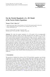
FLOWS WITH SURFACE TENSION 325arclength grid points using Newton's method and Fourierinterpolation. The equation that must be solved isfor flj as j=0(1)NLs,,d~'=~-~ s~,d~'=jh~-~n, (87)with h=2n/N. Here ~ is a givenparametrization, not necessarily arclength, and flj gives thelocation of points in the ~ parametrization that are equallyspaced in arclength. L is obtained by trapezoidal integrationofs~ over its period.Moreover, in the case of inertial vortex sheets, the unnormalizedvortex sheet strength in the arbitrary parametrization~, must be rescaled appropriately for use in the equalarclength frame. This is because in the inertial vortex sheetcase, the unnormalized vortex sheet strength appears in aframe-dependent way in the equations of motion, see (15)and (27). In particular, suppose that ~(~, 0) is given. Then,the initial data used in the equal arclength frame isy(flj, 0). fl~(jh), where fl~ is computed from the solution ofEq. (87) using the DFT. The true vortex sheet strength (i.e.,the tangential jump in velocity: 7/s~), on the other hand, isframe-independent. Of course, it is not necessary to rescalethe unnormalized vortex sheet strength in the Hele-Shawcase as it is not an independent variable and does, in fact,appear in a frame-independent way.The Forward Mapping (x, y) ~ (L, O)Recall that the tangent angle is given byO= tan-~(y~/x~). However, this is not a good formula touse numerically as it is tricky to ensure that the variation ofy~/x~ over the interface does not result in jumps in 0 due tobranching in the inverse tangent. It is better to construct 0from the curvature by integrating the formulaO~=s~K, where x=(x~y~-y~x~)/s]. (88)The constant of integration may be chosen by using theinverse tangent formula at the initial point of integration.The Inverse Mapping (L, 0) ~ (x, y)The difficulties in recovering (x, y) from (L, 0) are purelyimplementational; (x, y) are obtained by integrating theformulaeLLx, = cos(0), y~ = ~ sin(0). (89)For the flows that are periodic in x, the formulation requiresthat x = cc + p(0c, t) and y = q(~, t), where p, q are periodicin 0~. In particular, the coefficient of the linear term inmust be exactly 1 in the x coordinate and 0 in the ycoordinate. Unfortunately, integrating (89) using the DFTperturbs these coefficients slightly due to numerical error.Unchecked, this has a devastating effect on the code as theassumed periodicity of the solution is altered. The alternatingpoint quadrature role, for example, loses spectralaccuracy and the code becomes unstable. This difficulty iseasily fixed by forcing the coefficients to be exactly 1 and 0,respectively, after the reconstruction process. For example,we reconstruct x by using the discretization ofx(~,t)=x(O,t)+~I 1 L ~2~ doCl- Jo+ ~ cos(0(~')) d~'. (90)Of course, in the absence of numerical error, the explicitcoefficient of~ in (90) vanishes. We have considered otherways to enforce this condition, but we have found that justexplicitly forcing these coefficients to be 1 and 0, respectively,performs the best numerically. We remark that Strainalso noted this difficulty in [48], but he did not seem toemploy a correction of it computationally.7. SOME NUMERICAL RESULTSIn this section, the results of numerical simulations arepresented for several fluid interface problems. The first ofthese is the motion of Hele-Shaw interfaces, which evolveby a competition of surface tension and unstable densitystratification. The second is the expansion of a gas bubbleinto a Hele-Shaw fluid. The third is the motion of inertialvortex sheets, which evolve by a competition of surface tensionand the Kelvin-Helmholtz instability. And the fourth isthe motion of an interface with surface tension in anunstably stratified Boussinesq fluid. All of these simulationsuse the appropriate small scale decomposition, togetherwith the associated numerical methods discussed in theprevious section.The computations in the open geometry (i.e., all cases butthe expanding bubble) assume one-periodic interfacesrather than 2n-periodic as was assumed in the previous sections.The two are equivalent by a rescaling of time, space,and the physical parameters.7.1. Numerical Results: Hele-Shaw7.1.1. Numerical StiffnessThis section begins with a comparison of the stabilityconstraints of three methods for Hele-Shaw flow--thesecond-order linear propagator, the Crank-Nicholson/leapfrog, and the explicit second-order Adams-Bashforthmethod applied to small scale decomposition (62). Todemonstrate the constraints on these methods (especially

326 HOU, LOWENGRUB, AND SHELLEYfor the explicit scheme), it is sufficient to consider shorttimes and the simple initial conditionx(a, O) =~, y(~, O) = -0.01 sin 2m~. (91)Here, R =- 1 and S = 0.01 so that the flow is unstablystratified although k = + 1 are the only linearly growingmodes. A~ = 0 is taken for simplicity.For each method, Fig. 3 shows plots of the Fourier transformlOglo IP(k)l versus k at t = 0.1 for the two resolutionsN= 64 (top) and N= 128 (bottom). The results from theintegrating factor and Crank-Nicholson methods use thetimestep At = 0.01 at both spatial resolutions. Instability ina time-integration method is usually manifested as rapidand unphysical growth in the amplitudes of the highwavenumbermodes. As is clear from the spectrum, no timestep reduction is necessary for stability of either method asthe resolution is increased, at least at these resolutions. Forlarger values of N, i.e., N up to 2048, we do see theemergence of a first-order CFL constraint imposed by thetransport term. Although this constraint is not seen inthe near equilibrium linear analysis, as the transport term(see Eq. (53)) is neglected, it is not surprising that it is seenin the full computation for large N.The results for the explicit scheme are shown in the lastcolumn. The solid curve corresponds to t = 0.10 with At =2.0x10 -5 for N=64, and At=O.25xlO -5 for N=128.This reduction in time step is exactly the factor of 8 that is0-5logz0l:9(k)t-10-15-20 00-5loSxol~'(k)l-lOLin. Prop., (a)t=.10d~.01, N=6401-51-15t=.10C-N. (b)dt=.01, N=64w20 40 60 80 20 40 60 80kkt=.10(d)dt=.01, N=128C-5t=.10(e)dr=.01. N=128Explicit A-B, (c)0,._ t=.002, dt-=4.0d-5- t=. 10. dt=2.0d-5-5~ N=64-lOlli ,,"iii't i-15 ~-2C0 20•40 60 80k(00 - t=.0002, dt=0.5d-.*- t=.10, dt=O.25d-5-5 N=128-1C -10 t,II-15 -15 -15 r JJ i-20 ~0 20 40 60 80-2C0 20 40 60 80-200 20 40 60 80k k kFIG. 3. Hele-Shaw numerical stiffness: acomparison oflogl0 ]~(k)[ vsk at t=0.10 and R=-I, S=0.01: (a) linear propagator, N=64,At = 0.01; (b) Crank-Nicholson N= 64, At = 0.01; (c) explicit secondorderAdams-Bashforth, N= 64, At = 2.0 x l0 -5 and at t = 2.0 x 10 -3 withAt=4.0xl0-5; (d) lin. prop., N=128, At=0.01; (e) C-N, N=128,At=0.01; (f) explicit A-B, N= 128, At=0.25 x 10 -5 and t=2.0 x 10 -4with At = 0.5 x 10-st*stipulated by the near equilibrium stability constraint/it~ Ch 3. To demonstrate the proximity of the stabilitythreshold, the results are given also for computations usingthe intermediate time steps At = 4.0 × 10-5, at t = 0.002 forN= 64, and At = 0.5 x 10 -5, at t = 0.0002 forN= 128 (givenby the dashed lines). That the stability criterion is violatedis shown by the unphysical growth of the spectrum at highwavenumbers. The latter two computations cannot be continuedmuch beyond these times as the numerical solutionblows up.At these early times, the flow has not yet developed spatialcomplexity. Therefore, there are no significant aliasingerrors and hence no filtering is used in these calculations.Aliasing errors become especially important when the activeportion of the spectrum approaches and exceeds theNyquist frequency k = N/2. Finally, the explicit computationwith N = 128 and/It = 0.25 × 10 -5 takes approximately175 min on an IRIS Indigo workstation while the linearpropagator and the Crank-Nicholson computations eachtake less than 30 s (due to the fact that their time steps are/It = 0.01 each).7.1.2. Longer Time ComputationsConsider now the evolution from the multimodal intialconditionx(~, O) = a, y(~, O) = 0.01 cos 2zr~ - 0.01 sin 6try, (92)with S= 0.1, R = -50, and A, = 0. Now, the modes [k[ ~< 3are linearly unstable, and the competition between the sur-20-1-2(a)-0.5 0 0.5 1 1.5t=0(d)1110-1(b)-0.5 0 0.5 I 1.5t=0.04(e)-0.5 0 0.5 1 1.5 -0.5 0 0.5 1 1.5t=0.08t=0.10o{-2}17, )/1"65 I(c)-0.5 0 0.5 1 1.5t=0.061.6 ]1.55I(f)1.5 I0.75 0.8 0.85t=0.10FIG. 4. Long-time evolution of a Hele-Shaw interface: S=0.1,R = -50, N= 2048, At= 3.125 x 10-5: (a) t= 0; (b) t= 0.04; (c) t= 0.06;(d) t = 0.08; ( e ) t = 0.10; (f) close-up of topmost pinching region, t = 0.10.

FLOWS WITH SURFACE TENSION 327face tension and the unstable stratification causes the interfaceto rapidly develop a ramified spatial structure.A time sequence of inteface positions is shown in Fig. 4using N=2048 and At= 3.125 × 10 -5. The second-orderlinear propagator method is used, and the time step ischosen small enough so as to effectively eliminate time-steppingerrors from the computation. At early times, threerising and falling fingers of fluid form. As time progresses,the tips of these fingers thicken and begin to resemblebubbles. The necks of the fastest moving fingers begin tonarrow and their sides approach tangentially. The othernecks appear to follow suit. These necks become localizedjets, fluxing fluid from the bulk into the bubbles. At latertimes, the sides of the necks seem to self-intersect or pinch.However, a close-up of the neck region (box (f)) of thetopmost bubble reveals that the pinching has not yet takenplace by t = 0.10 and that the neck still has a nonzero width.As the necks narrow, however, it becomes more and moredifficult to maintain resolution. This is because the alternatepoint discretization of the Birkhoff-Rott integral requires aminimum width of six or seven grid lengths in the neckregion for accuracy [ 8 ]. This effect is illustrated in Fig. 5,where the interface positions are compared at t = 0.10 withN= 1024 and N---2048. Although pinching has alreadytaken place in the N = 1024 calculation, it is unphysical. Therrrinimum width of the neck as a function of time is shownin Fig. 6 for several spatial resolutions: N= 512, N= 1024and N=2048 (again using the same time step Lit=3.125 x 10-5). The width is computed by minimizing thedistance function between the bounding curves, which arerepresented by Fourier polynomials. The width of the neckdecreases rapidly at early times. By t = 0.065 with N= 512,the neck is but one grid length wide, and the calculationbecomes inaccurate. The higher resolution calculations21.510.50-0.5-1-1.5-2 1024i0LiI 2FIG. 5. Comparison of Hele-Shaw interfaces at t = 0.10 for differentspatial resolutions: the left corresponds to N= 1024 and the right toN=2048; S=0.1, R= -50, At= 3.125 x l0 -5.)L32O480.12-- 512-.- 10240.1 - 20480.08~ 0.0~0.0,t0.020 5 6 7 8 :, 10T x 10 .2FIG. 6. Minimum distance to pinching for N= 512, N= 1024, andN= 2048; S = 0.1, R = -50, At = 3.125 x 10 -5.indicate that the narrowing slows shortly thereafter.However, by t = 0.08, the N = 1024 calculation has a neckwidth of only five grid lengths, and that calculation becomesinaccurate. But by using N = 2048, the width is seen tosaturate after t= 0.08 and shows only a slight furtherdecrease by t = 0.10. The neck region is 11 of its grid lengthswide. Presumably, the width of the neck region scales withthe surface tension, although this has not been studied indetail.This lack of self-intersection in the neck region is consistentwith behavior found by Goldstein, Pesci, and Shelley[ 18 ] in asymptotic models of jets in Hele-Shaw flows. Theirmodelling suggests also that the minimum neck widthdecreases by a factor of two with a fourfold decrease in thesurface tension. It is only in the limit of zero surface tensionthat their model equation predicts the breaking of the neck.They do consider other cases, however, where the surfacetension does not prevent the pinching of material interfaces.Figure 7 shows the evolution of the curvature. The topleft plot shows the inverse of the maximum absolute curvature.Vanishing in this plot would correspond to adivergence of the curvature. At early times, there is a rapidincrease in the curvature (a decrease in the plot). It peaksaround t= 0.015 and then begins to decrease. This lastsuntil t -- 0.05. The curvature then refocuses and the processrepeats itself several times. By the end of the computation,the curvature has nearly reached again its peak at t = 0.015.The other plots in Fig. 7 show x as a function of ~ at severaltimes; these graphs indicate that in fact, the curvaturesaturates at one part of the interface and refocuses inanother, leading to a very complicated overall structure.The boundaries of the narrow neck regions are indicated bya pairs of closely spaced peaks of like signed curvature. Thephenomenon of saturation and refocussing will be seenagain in the context of inertial vortex sheets.

328 HOU, LOWENGRUB, AND SHELLEY0.250.20.150A0.05Inverse Curvature, (a)20110101Curvature, (b)0 0.05 O. 1 0.5TT=0.02Curvature, (d)20 20110-10101O~ilCurvature, (e)Curvature, (c)-200 0.5 0.5-200.5T--0.06 T--0.08 T--0.10200-10-20 0 0.5T---0.04200-10Curvature, (f)FIG. 7. Time evolution of the curvature; S = 0.1, R = -50, N = 2048,At= 3.125 x 10-5: (a) plot of inverse maximum of curvature (absolutevalue); (b) curvature at t=0.02; (c) t=0.04; (d) t=0.06; (e) t=0.08;(f) t = 0.10.Error Analysis. In Fig. 8, spatial convergence isdemonstrated by comparing computations using N= 256,512, and 1024 with those from N= 2048. The time step isAt = 3.125 × 10-5 for all resolutions. The error is measuredas eN(t) = maxj Ixj(t; N) - xj(t; 2048)1, where Nis the numberof points in the lower resolution calculations. The erroris plotted on a negative logarithm (base 10) vertical scale.The error is consistently around 10- lO, for each of the lowerresolutions, until the interfaces nearly pinch. Then, rapidlosses of accuracy are seen from about t = 0.03 for N = 256,~ 6"712 ~ ~ . _ _113842Ci0.01 0.02 0.(13-- 256-~ -.- 512i~ - 1024' ~ .,\~,, ,.\,i .ii i i i i . . . . . i'- ....0.04 0.05 0.06 0.07 0.08 0.09 0.1TFIG. 8. Error in x-coordinate (-loglo(error)); S=0.1, R=-50,Jt = 3.125 x 10-5, exact solution approximated by N= 2048.t=0.05 for N=512, and t=0.07 for N= 1024. It is clearthat more resolution will be required for further computationof this flow. Further, as the quadrature we use is thechief culprit in loss of accuracy, it would be useful to considerother types of quadrature (i.e., product integrationmethods) that do not lose accuracy so catastrophicallythrough the close approach of interfaces. The second-ordertemporal convergence can be shown similarly, but it is notpresented here.7.1.3. The Expanding BubbleThe calculation of a gas bubble expanding into aHele-Shaw fluid, shown in Fig. 1, is now briefly discussed.The dynamics of expanding bubbles in the radial geometryhave attracted a great deal of attention due to the formationof striking patterns observed in experiments (see the manyreferences and contributions in [47 ], for example). In thisflow, an expanding, unstable interface is produced byplacing a mass source at the center of the bubble. Linearizationabout an expanding circular bubble, with radius R(t)and pumping rate dA/dt, gives the instantaneous growthrate [ 16 ]1(dA/dtak(t) =R--~ (k- 1) --2reS\-- (k- 1)k(k+ 1)).R(t)(93)The pumping term replaces the gravitational term in theprevious example as the source of instability. For a constantpumping rate (here dA/dt=2g) we obtain a Mullins-Sekerka type instability, which shows the competitionbetween the destabilization effect due to pumping and thestabilizing effect due to surface tension.Unlike the previous calculation, there is now a viscositycontrast (A, = 1,/t = 0 inside the bubble). Consequently, anintegral equation analagous to Eq. (20) must be solved forthe vortex sheet strength y (see Dai and Shelley [ 16 ] ). Here,the integral equation is solved in its dipole form, forthe dipole strength v, which is related to y by ? = v~ (seeGreenbaum, Greengard, and McFadden [22]). Theintegral equation is solved iteratively using the GMRESmethod [42]. Birkhoff-Rott type integrals over a closedinterface (although with smooth kernels) must be evaluatedat each step. The fast multipole method [23] is used toevaluate them. Thus, at each iteration, the operation countis O(N) as opposed to O(N 2) for direct summation. Theconvergence tolerance for the GMRES iteration is set to10-x2. The rate of convergence is improved considerably bya simple diagonal preconditioning, as used in [22], and bysupplying a good first guess through an extrapolation ofsolutions at previous time steps. Once the solution to theintegral equation is obtained, the Dirichlet-Neumann mapis used to determine the normal velocity of the interface.

FLOWS WITH SURFACE TENSION 329This results again in a Birkhoff-Rott type integral (nowwith a singular kernel) that must be evaluated and alternate 3point quadrature using the fast multipole methods is2.5employed to this end. See [ 16, 22] for details. Time integra-2~ a5tion is accomplished using the second-order linearpropagator method on the small scale decomposition; i.e., -~the method is given by Eq. (69) where the term A ~ is 0.5modified to account for a pumping term (see [ 16 ]). The 0method is spectrally accurate in space.The initial condition is given by2.42.2Log-Log plot of A(t) vs. G(t), area vs. radius of gyration, (a).J0 0.1 0.2 0.3 0.4 0.5 0.6 0.7 0.8 0.9log10 G(t)Plot of Slope, (b).(Xo(~), yo(~)) = r(~)(cos 0t, sin a)with r(0~) = 1 +0.1 sin 20t+0.1 cos 30t (94)and is shown as the innermost curve of Fig. 1; it imposes noparticular symmetry on the ensuing motion. The value ofthe surface tension is S = 0.001. At t = 45, the time step isAt = 0.0005 and N= 8192.Figure 1 shows the expansion of this bubble from t = 0 upto 45, at unit intervals of time. This simulation displaysmuch of the behavior that has stimulated interest in patternformation in Hele-Shaw flows. An early times, three main"l]ords" form in the interface. These t]ords separate threeexp"anding fronts. The number of fjords arises from the k = 3component in the initial data. The expanding fronts rapidlydevelop oscillations, particularly along their outer edgesnear the t]ords, which themselves form "fingers" and"petals." The petals expand outwards and eventually tipsplitinto two petals. Although this tip splitting temporarilyrestabilizes them, the process repeats itself. One petal in thesecond quadrant has already tip-split four times and isapproaching a fifth tip-splitting. There is also abundantevidence of competition between these various structures.Of the approximately 25 protuberances that develop atearly times (say between t = 5 and 8), only about 15 of themare still actively growing outwards as t = 45. The remainderhave either stopped growing outwards, or have receded andbeen absorbed back towards the main bulk of the bubble.Although further details of these calculations will appearelsewhere, we present one interesting diagnostic. Figure 9shows the bubble area A(t) versus G(t), the "radius of gyration,"on a log-log scale (upper graph). G(t) is defined as themaximum distance of a point on the interface from the injectionpoint. It is computed numerically by maximizing theFourier interpolant of the distance function from the origin(the injection point) to the interface. The radius of gyrationhas been used as a measurement of complexity, as the slopeof log G versus log A, shown in the middle and lowergraphs, gives roughly a dimension d; where d is the dimensionof the bubble (i.e., A ~ Gd). For example, the slope istwo for a circular bubble. This slope is, of course, notsmooth, as the point of maximum radius jumps between dif-2o 1.81.61.41.2 0 5 10 15 20 25 30 35 40 45TimeFIG. 9. (a) The bubble area A(t) vs the radius of gyration G(t) on alog-log scale. (b) The points are the slope (dimension) dmeasured from (a)as a function of time. The dashed lines are at d= 1.66 and 1.71 (DLAestimates).ferent sites during the evolution. The jumps themselves areassociated typically with tip-splitting events, as the splittingallows a newly formed finger to move outwards morequickly. The dashed lines have the values 1.71 and 1.66 (see[53, 26], respectively), which are estimates for the fractaldimension of a branched object grown via diffusion limitedaggregation (DLA), a prototypic model for the growthof branched structures [53]. There is a short period(15

330 HOU, LOWENGRUB, AND SHELLEYspectrum had risen to 10 -8 (from 10-16). The N= 8192computation was stopped at t = 45, even though its highmodes had risen to only 10-11. We note that the computedarea of the bubble at t = 45 still agrees to six digits with itsexact value.The calculation to t = 25.0 took about 9 days on anIBM R6000 workstation. Had there been no accompayingintegral equation to solve, it would have taken but a fewhours. The best approach to reducing this time appears tobe finding better preconditioners for the iteration. Previouscalculations of similar flows have been performed [ 15, 16].The time step here is 103 times larger than that used by Daiand Shelley [ 16 ] in computations of a similar flow using anexplicit method with a lesser number of points, and theinterface here has developed far more structure. Further, nosymmetries have been imposed. Again, further details willappear elsewhere.7.2. Numerical Results: Inertial Vortex SheetsIn these last two subsections, we examine the long-timeevolution of inertial vortex sheets with surface tension, bothin a homogeneous fluid and in a fluid with slight densitystratification. Leaving aside issues such as dimensionalityand viscous effects, the first case is not a completely artificialsituation. Two immiscible fluids can be density matched andstill produce a surface tension. Further, in the absence ofsurface tension, the singularities of a vortex sheet embeddedwithin a homogeneous fluid give the basic form of thesingularities observed on an interface evolving by theRayleigh-Taylor instability [ 5 ]. Our results in the last subsectionsuggest that this still holds true with the addition ofsurface tension.Computationally, such problems have also been consideredby Pullin [ 38 ], by Rangel and Sirignano [ 39], byBaker and Nachbin [7], and by Beale et al. [ 10, 12]. Pullinused a method based on cubic splines and observed apersistent numerical instability that was only slightlyameliorated by additional smoothing of the interface position.His calculations are restricted to short times. Rangel etaL used a similar method, combined with a remeshing, usinglinear interpolation of the interface positions and sheetstrength, at every time step. This is strongly smoothing.Indeed, they calculate the smooth roll-up of the sheet, evenwithout surface tension, for which it is known that asingularity interrupts the motion well before roll-up occurs[33, 31, 44]. Baker and Nachbin and Beale et al. investigatethe stability of spatial discretizations. In these works, theissue of stiffness is not addressed, and the calculations areagain restricted to short times.7.2.1. Numerical StiffnessIn this section, the stability constraints are compared forthe second-order linear propagator, Crank-Nicholson/leapfrog, and explicit second-order Adams-Bashforthmethods for small scale decomposition of the 0 - L formulationof inertial vortex sheets, Eqs. (55) and (56). For theexplicit scheme, the Adams-Bashforth discretization is usedin all three equations. The initial condition isx(~, 0) = ~ + 0.01 sin 2zt~, y(ct, 0) -- -0.01 sin 2~,7(~, 0)= 1.0.(95)This initial data was used by Krasny [31] in the absence ofsurface tension. In that case, a curvature singularity forms att ~ 0.375. The calculations here have S = 0.005, which gives16 linearly growing modes in the period.Figure 10 shows plots of log10 IP(k)F for the threemethods with N = 64 and N= 256 at t = 0.12. This is a factorof 4 increase in N, and so the near equilibrium constraintAt < Ch 3/2 requires a factor of 8 decrease in time step. Theresults from the Crank-Nicholson/leapfrog scheme aregiven in the first column. The time step At = 0.01 is used forboth resolutions and this scheme is clearly stable. As thereis little spatial complexity (i.e., no large aliasing errors),filtering has not been used. The results from the explicitAdams-Bashforth scheme are given in the middle column.The +-curves correspond to At = 3.1 x 10-4 for N = 64 andAt = 3.9 x 10-5 for N= 256. This is again the factor of 8 aspredicted by the stability constraint. The solid lines showthat the time step constraint is violated with At = 1.2 x 10 -3with N= 64 and At = 7.8 x 10-5 with N = 256. In the thirdcolumn of the figure the results are from the integratingl°glol$'(k)!l 0C-N, (a)° i , t=.12, N=64I-15 ~I]- dt=.01o-5-IO-15Expficit A-B. (b)t=. 12, N=64- dt=l.2d-3+ dt~3.1d-4Lin. Prop., (c)-2c-20 I50 1000 50 100kkk-2C-2-2050 100 50 I00 0 50 100k k k(d)(t=.12, N=256(g)t=.12, N=256(Dt=.12, N=256-5 - dt=.01- dt=7.Sd-5- dt=9.Sd-6-5+ dt=3.9d-5logaol~'(k)l-K-15-10:-10-15-10-15t=.12, N=64- dt=6.3d-4+ dt=l.6d-4FIG. 10. Inertial vortex sheet numerical stiffness: a comparison oflog10 I~(k)l vs k with S= 0.005 at t = 0.12: (a) Crank-Nicholson, N= 64,At = 0.01; (b) explicit second-order Adams-Bashforth, N= 64, At =1.2 × 10-3, 3.1 x 10-4; (c) linear propagator, N= 64, At = 6.3 x 10-4,1.6x 10-4; (d) C-N, N=256, At=0.01; (e) explicit A-B, N=256, At=7.8 x 10-5, 3.9 × 10 -5; (f) lin. prop., N= 256, At, At = 9.8 x 10-6.

FLOWS WITH SURFACE TENSION 331factor method. The stability region of this scheme does notdiffer significantly from that of the explicit scheme. This issomewhat surprising but confirmed by near equilibriumanalysis of the second-order linear propagator scheme.Other time discretizations, such as fourth-order Runge-Kutta, for the linear propagator method are currently beingstudied.By virtue of its stability, the Crank-Nicholson method isabout 250 times faster than both the explicit and linearpropagator methods with N = 256. Calculations with up to8192 points will be presented for the Crank-Nicholsonmethod. Following this scaling, the explicit Adams-Bashforth and the linear propagator Would require a timestep 4 x 105 times smaller.7.2.2. Long-Time ComputationThe long-time evolution of the initial data (95) withS=0.005 is now studied, using the Crank-Nicholsonscheme, together with filtering. The effect of the filtering isdiscussed in detail below.In Fig. 11, a time sequence of interface positions is given,starting from the initial condition. The calculation usesN= 1024 and/It = 1.25 x 10 -4. At early times, 0 ~< t < 0.40,the interface steepens and behaves similarly to the zero surfatetension case. It passes smoothly through the S--0Kelvin-Helmholtz singularity time (t ~0.375). At t=0.45,the interface becomes vertical at the center. It subsequentlyrolls over and produces two fingers (t ~ 0.50). These grow inlength in the sheet-wise direction (box (b)). The tips of thefingers broaden and roll with the sheet. This is clearly seenat t = 0.80 and there is evidence of capillary waves, seen aswiggles along the sheet. By t = 1.20, the sheet producesanother turn and the fingers have become broader andlarger. Additional capillary waves also have been producedand they traverse the interface outwards from the centerregion. This is a dispersive effect of the surface tension thatis seen more clearly in plots of the curvature and vortexsheet strength. Note that the part of the interface (on theinner turn) closest to the fingers has become quite flat andbends very slightly towards the fingers. At later times, thispart bends even more towards the fingers, the tips of thefingers narrow and both pieces of the interface approacheach other. At t--1.40, the interface appears to self-intersect,but a close-up of the region at this time indicates thatthere is still a finite distance between the upper finger andthe inner roll. The same is true for the lower finger by symmetry,although that symmetry is not imposed in thesimulation. At this time, the gap is but five grid lengths wide,and the calculation is stopped here. The length of the interfacehas more than doubled (a factor of 2.6).This type of self-approach is quite different from that seenin the Hele-Shaw flow. Here, each part of the interfaceappears to form a finite angle during the approach, whereasfor Hele-Shaw, the approach is tangential. The mechanismdriving the interface to self-approach is not yet well understoodand is under active study. Rather than ultimatelypreventing the pinching, as is apparently the case inthe Hele-Shaw jet flow, surface tension appears to push theflow further towards it by producing a jet through thenarrow gaps between the fingers and the inner turn ofthe spiral. Fluid streams into each of the fingers and the°i[-0.2 t-0.2(a)0 0.2 0.4 0.6 0.8T=0(c)(b)0 0.2 0.4 0.6 0.8T=0.60(d)0 0.2 0.4 0.6 0.8 0 0.2 0.4 0.6 0.8T=0.80T=I.20(e)(f)0.I(a)4-!f-4 ' '0 0.2 0.4 0.6 0.8T=0.0(c)4 ' ' '0 0.2 0.4 0.6 0.8T=0.80(¢)44(b)-4 , ,0 0.2 0.4 0.6 0.8T~.~(d)4-i0 0.2 0.4 0.6 0.8T=1.20(t)0 0.2 0.4 0.6 0.8 1 0.4 0.45 0.5 0.55T=l.40T=l.40FIG. 11. Inertial vortex sheet; sequence of interface positions:S= 0.005, N= 1024, z/t= 1.25 x 10-4: (a) t=0; (b) t =0.60; (c) t=0.80;(d) t = 1.20; (e) t = 1.40; (f) close-up of top pinching region, t = 1.40.- top-40 0.2 0.4 0.6 0.8 0 0.2 0.4 0.6 0.8T= 1.40 T= 1.40FIG. 12. Inertial vortex sheet: sequence ofy vs. ~t; S = 0.005, N= 1024,dt=1.25×10-4: (a) t=0; (b) t=0.60; (c) t=0.80; (d) t=l.20;(e) t = 1.40; (f) strength on opposite pieces of the upper pinching region,t = 1.40.

332 HOU, LOWENGRUB, AND SHELLEYtwo pieces of the interface are drawn togetherl This jet is 0.2recognized in that the approaching parts of the interfacecome with oppositely signed vortex sheet strengths, andtheir signs are such that fluid flows into the fingers. For thisinitial data (single-signed sheet strength), such a sign 0change in the vortex sheet strength can only occur in thepresence of surface tension.Figure 12 shows the unnormalized vortex sheet strength,~, versus 0~. Recall that y, initially, is not identically equal to1 as it has been rescaled appropriately for the 0- L frame.In this frame, the unnormalized vortex sheet strength differsfrom the true vortex sheet strength (i.e., the tangential jump 0in velocity) by only the time-dependent scale factor L/2zc. Atearly times, two positive peaks form in the vortex sheet 20ostrength (see box (b)). These are the remnants of the S = 0,Kelvin-Helmholtz instability, which concentrates vorticity 0into the center. In the S = 0 case, there is only one peak[31] but the addition of a small surface tension splits it in -20%two. There are small waves that form at the outer edges ofthese peaks and are presumably dispersive waves producedby the surface tension saturation of the Kelvin-Helmholtzinstability. At t = 0.80 (box (e)), the peaks have saturatedand more waves have been produced. These disperseoutward along the interface. The strength ? has also formeddownward peaks at the edge of the wave packet. The saturationand dispersion continues through t--1.20 (box (f)).However, when the interface begins to self-approach, thevortex sheet strength refocusses, forming the jet. By the finaltime t = 1.40 (box (e)), two pairs of positive and negativepeaks of vortex sheet strength have formed in each pinchingregion. These peaks have been isolated for the top pinchingregion in box (f). The top of the pinching region (inner turnof the spiral) comes with a negative signed vortex sheetstrength and the bottom comes with a positive sign. Thisimplies that fluid is streaming through the gap towards thecenter and into the downward pointing finger.Saturation and refocussing is also observed in the curvature.Its evolution is plotted in Fig. 13. The first graphshows the inverse maximum of the curvature (in absolutevalue) as a function of time. There is an initial region ofrapid growth in the curvature (decrease in the plot) due tothe S = 0 Kelvin-Helmholtz instability. Recall that for theKelvin-Helmholtz singularity, the curvature diverges. Here,the curvature saturates and eventually refocusses. By thefinal time t = 1.40, the maximum of the curvature nearly ~reaches that attained during the initial period of growth. 4The refocussing, however, occurs at different places alongthe interface as seen in the other plots of t¢ versus ~. Disper- 2sive waves are also generated and move outwards along theinterface. At t = 1.40, the pinching points are indicated bypairs of like-signed peaks in the curvature.Evidence is now presented to show that the pinchingtakes place in a finite time. Maintaining resolution is criticaland so the neck widths obtained from different spatial and0.I ~ , ~i1c8Inverse Curvanu~, (a)0.5 ITCurvature, (c)-200 . . . .0.2 0.4 0.6 0.8T=0.60Curvature, (e)J ~0.2 0.4 0.6 0.8T=l.201.5Curvature, (b)-200~ 0.2 0.4 0.6 0.8T=0.40Curvature, (d)-2000 0.2 0.4 0.6 0.8T=0.800Curvature, (O2o00 o~ o-q" o-g o-~T=I.40FIG. 13. Inertial vortex sheet: sequence ofx vs. a; S = 0.005, N= 1024,A t = 1.25 x 10 - 4: (a) plot of inverse maximum curvature (absolute value ):(b) plot of curvature, t=0.40; (c) t=0.60; (d) t=0.80; (e) t= 1.20;(f) t= 1.40.temporal resolutions are compared. This is shown in the topgraph of Fig. 14, which shows minimum width in the toppinching region, graphed as a function of time starting att = 1.40. As in the Hele-Shaw case, the minimum width iscomputed by minimizing the distance function betweeneach piece of the interface and using the Fourier interpolant1.4x 10 -3Minimum Distance to Pinching, (a).. 1024-- 2048-.- 4096- 81921.405 1.41 1.415 1.42 1.425 1.43 1.435TNumber of Accurate Digits in Energy, (b)- 2048 ............................... - ._ '.~.. 1024-- 5120.2 0.4 0.6 0.8 I 1.2 1.4TFIG. 14. Pinching in, and accuracy in the energy of, the inertial vortexsheet: (a) minimum width of the top pinching region: S= 0.005; N= 1024with At = 2.5 x I0-4; N = 2048 with At = 1.25 × I0-4; N= 4096 with At =6.25 x 10-s; N=8192 with At=3.125 x 10 -5. (b) Number of accuratedigits in the energy: S=0.005; N=512, N= 1024, N=2048 with At=1.25 × 10-4, and N= 1024 with At = 3.125 × 10 -5 (1024ext).

FLOWS WITH SURFACE TENSION 333of the curve. The spatial resolutions shown are N= 1024with At=2.5xlO-4, N=2048 with At=1.25xlO-4,N=4096 with At=6.25 x 10 -5 , and N=8192 with At=3.125 x 10-5. The computations with N= 2048 and aboveare computed by restarting Fourier interpolants of lowerresolutions. In particular, the N= 2048 computation isrestarted from the N= 1024 computation at t = 1.25. TheN=4096 and N= 8192 computations are restarted fromN = 2048 at t = 1.40. These are times at which the active spatialspectrum of the lower resolution calculations begin toapproach the Nyquist frequency. Additional details of thesecalculations will appear in a separate study [ 28 ].In Fig. 14a, it is seen that the time of pinching is adecreasing function of resolution and strongly suggests thatpinching occurs at a finite time. Moreover, the width seemsto vanish with an infinite slope, implying that the pinchingrate intensifies as the width narrows. Again, further detailswill appear in [ 28 ].This apparent singularity is of a completely different typethan that of the S = 0 Kelvin-Helmholtz singularity. Here,the singularity is a topological singularity and may signal animminent change in the topology of the flow. The curvature,vortex sheet strength, and fluid velocity all apparentlydiverge at the pinching time [28]. In the S = 0 case, it is thevelocity gradient (strain rate) and the curvature thatdiverge, but not 7- More fundamentally, with S = 0 thesingularity occurs through a rapid compression of vorticityalong the sheet at a single isolated point [33, 31, 9, 44].Here, the divergence occurs through a rapid production ofvorticity that is associated with the pinching. In a separatestudy, we will show evidence this collapse is a localphenomenon in the flow and satisfies a scalingbehavior [28]. We have also derived localized equationsand they are currently under investigation.Error Analysis and the Role of Filtering. We now turn toan analysis of the errors in our scheme, first by consideringthe energy E(t), which is a conserved quantity not conservedby the discrete methods. The energy E is the sum of the perturbationkinetic and the interfacial energies, given bywhereis the interfacial energyE( t) = Es( t) + Ek( t), (96)Es(t) = S(L - 1 ) (97)1Ek(t) = ½ fo ~,(o~', t) ~(od, t) d~' (98)is the perturbation kinetic energy and ~k is the stream function,ff(~, t) = - 2-~ Re {f2 Y(c(, t)× log[sin rc(z(oq t)- z(~', t))] do(}. (99)The formula for ff can be rewritten, by explicitly subtractingoff the logarithmic singularity and integrating by parts, toyield an expression that can be computed with spectralaccuracy numerically. See Pullin [38] and Baker andNachbin [ 7 ] for details.The lower graph of Fig. 14 shows -lOgl0 [(E(t)-E(O) )/E(O ) I for several spatial resolutions. This is essentiallynumber of accurate digits in the energy. The time step isAt= 1.25 x 10 -4 for all the resolutions except the onemarked 1024ext. This uses At= 3.125 x 10 -5 and uses asinitial data the other N= 1024 computation at t = 0.40.Prior to the time t = 0.40, there is essentially no differencebetween the different resolutions and the errors aredominated by the time stepping. Over nine digits ofaccuracy are obtained. Around t = 0.42, there is a suddenoverall decrease in accuracy. This is an effect from the S = 0Kelvin-Helmholtz singularity. This decrease is primarilydue to time stepping since the N= 512, 1024, and 2048 curvesall lie on top of one another immediately afterwards.This is reinforced by the 1024ext curve which has a fourtimes smaller time step and lies well above the others. Fromt = 0.43 until nearly the end of the computation, the energychanges only slowly, and the N = 1024 and 2048 computationsare slightly more accurate than the N= 512. Aroundt = 1.40, when the pinching begins to take place, there isanother sudden loss of accuracy and now N = 2048 is moreaccurate than N= 1024 as spatial resolution becomes veryimportant.In view of these results, our code would certainly benefitfrom adaptive time stepping. A small time step is really onlyneeded near the Kelvin-Helmholtz singularity time andnear the time of pinching. Larger time steps could likely beused safely for the remainder of the computation. Finally,we remark that the energy of the N= 8192 computationused to compute the pinching distance still has over sixdigits of accuracy at the pinching time [ 28 ].Since the energy is an integral quantity, using it tomeasure error is smoother than using a pointwise error. Asin the Hele-Shaw case, we also consider the pointwise errorin the x-component of the interface position. In Fig. 15,-lOgl0(e~t)) is plotted (see the Hele-Shaw results for adefinition of eN), with the N = 2048 calculation again usedas an approximation of the exact solution. Several resolutionsare graphed and all use the time step At = 1.25 x 10-4.This graph is qualitatively similar to that of the energy anddemonstrates the spatial convergence of our scheme. Thetemporal convergence can be similarly shown, but is notpresented.

334 HOU, LOWENGRUB, AND SHELLEYle',io L,~8• -r64 ,-.',;iI-1024-.-512--256t-J . . . . . . . . . . . . . . . . . . . _.,ItI2 012 0'.4 0'.6 018 ; 1;~ 1.4TFIG. 15. Error in x-coordinate; S=0.005, At= 1.25 x 10 -4, exactsolution approximated by N = 2048.The role of Fourier filtering (H in Eq. (86)) is nowdiscussed. As the higher Fourier modes rise above theround-off level (due to nonlinear interaction), an aliasinginstability appears. This instability can be controlled byeither increasing the resolution or by using some kind offiltering. Both have been tried, and we conclude that it ismore practical to use a high order Fourier filtering thatsmooths the highest modes. By this, it is possible to achievethe same level of accuracy, at late times, using many fewerpoints than would be required without it. This is seen mostdirectly by comparing their energies.Figure 16 compares the energies of calculations both withand without filtering on the time interval 0.4 to 0.6. Recall-'xthat the filtering combines the Fourier and Krasny filters.The effect of Krasny filtering is discussed below. This is avery good test, as the spectrum is broadly populated due tothe effect of the S= 0 singularity. The time step is At =1.25 x 10-4 for all the calculations. The filtered calculationsshow a generally slower loss of accuracy and are moreaccurate than their unfiltered counterparts by t = 0.46. Infact, at t = 0.46, the N= 256 filtered calculation is moreaccurate than the unfiltered N= 1024 computation! Theunfiltered computations both break down before t = 0.6.The aliasing instability can be observed directly in spectralplots of the numerical solution. In Figs. 17a, b areshown the y-spectra of the filtered and unfiltered computations,respectively. In Fig. 17b, the aliasing instability isclearly seen through the artificial rise in the high wavenumberspectrum at t = 0.46. The unfiltered calculation cannotbe continued long after this time, as this rise causes the codeto blow up. The filtered computation, on the other hand,does not exhibit such a rise. Moreover, it is really only thelast few modes that are damped by the filtering (modes450-512). Since Krasny filtering is also employed in thefiltering method, the modes at the roundoff level 10 -]6 inthe unsmoothed calculation are set to zero in the smoothedone. They are seen at the 10 -19 level in the plot (this keptthe logarithm function in the graphics package fromdiverging). Moreover, it is clear from the behavior of thespectrum of the unfiltered computation that roundoff errorsgrow rather slowly and, therefore, the main effect of Krasnyfiltering is to keep the spectrum clean and is not necessaryfor stability.The spectrum also indicates a very interesting behavior.At the early times 0 ~< t ~< 0.46, energy is rapidly moved tothe high wavenumbers due to the near Kelvin-Helrnholtz108:~ 64Number of Aecttrate Digits in Energy, (a)256-- unfiltered20.4 0.42 0,44 0.46 0.48 0.5 0.52T(b)108:g 64"" 10245121024256-- unfiltered- filtered0.54 0.56 0.5820.4 0.42 0.44 0.46 0.48 0.5 0.52 0.54 0.56 0.58TFIG. 16. Accuracy in energy: filtered vs unfiltered, S= 0.005, At =1.25x 10-4: (a) filtered vs unfiltered, N=256, 512, 1024; (b) filtered(N= 512) vs unfiltered (N= 1024).0Filtered C-N, (a)loga01#(k)l- I C 1 ~ - -t=0,42 ~ t=0.46"2G0 100 200 300 400 500 600kUnfiltered C-N, (b)0log10lP(k)l- 1 0 ~ ~---------~ t=0.46 tlogloJ~'(k)l-20 0 100 200 300 400 500 600kFiltered C-N, Later Times, (c)p=1.20 r-20 0 100 200 300 400 500 600kFIG. 17. Log plot of power spectra (log [~(k)l ) at different times,S = 0.005, At = 1.25 x 10 -4, N= 1024: (a) filtered Crank-Nicholson, shorttime; (b) unfiltered C-N, short time; (c) filtered C-N, long time.

FLOWS WITH SURFACE TENSION 335singularity, and at t--0.46 all the modes lie above theround-off. Then, as seen in Fig. 17c, energy begins to movefrom high wavenumbes back to low wavenumbers. Forexample, the highest nonzero mode at t--0.60 is aboutk = 450 and by time t = 1.20, it moves to about k = 360. Thisbehavior reflects the saturation observed in 7 and x.Between t = 1.20 and t = 1.40, the energy resumes its generationat high wavenumbers (refocussing) and by t = 1.40, allmodes again lie above the round-off.7.3. Boussinesq InterfacesIn this section, a preliminary long time computation ofan interface in an unstably stratified Boussinesq flow ispresented. In Boussinesq flow, the fluids are only weaklystratified across the interface and the only contribution tovorticity production is through the buoyancy term. Weremark that Boussinesq interface flows in the absence ofsurface tension develop finite time singularities of a formwell described by those for inertial vortex sheets withoutsurface tension [ 37, 5 ]. The 7 evolution equation isV,-~3~((T-W.s)7/s~)=Sx~-2Ry~. (100)The term Q in the small scale decomposition (56) is replacedb'y Q-2Rye. The Crank-Nicholson scheme is used withfiltering for the same initial data in x and y as in the inertialvortex sheet calculation. Initially, 7 = 0. Further, R = -- 5 sothat the flow is unstably stratfied, and there are 19 linearlyunstable modes.Figure 18 shows the time evolution of two periods of the0.5.0.05 - -(a)0 0.5 1t=01.5 2(c)0.5(b)0 . 5 ~ 0-0.50 0.5 1 1.5T=0.60(d)0.501-0.5 0 0.5 1 1.5 2 0 0.5 1 1.5T=0.70T=0.80(e)(f)0.5 0.10 0.5 1 1.5 2 0.15 0.2 0.25 0.3T--0.89T=0.89FIG. 18. Evolution ofa Boussinesq interface; S = 0.005, R = - 5, At =3.125x 10 -5 , N= 1024: (a) t=0; (b) t=0.60; (c) t=0.70; (d) t=0.80;(e) t = 0.89; (f) close-up of a left-most spiral, t = 0.89.0.35interface. This computation uses N=1024 and At=3.125× 10 5. The classical Rayleigh-Taylor structure isseen as two spirals form on either side of the fluid plumes.The spirals are smaller than those for the inertial vortexsheet, but an examination of their inner structure showsthem to be very similar. In particular, note the inward bulgein the second turn of the interface (t = 0.89, close-up). Itseems very plausible that there will again be finite timepinching. One consequence of these smaller spirals is thatthis flow is more difficult to resolve than the previous caseof inertial vortex sheets. More highly resolved computationswill be presented in a separate study [28].An intriguing question is whether such "bubble" formation,as is apparently predicted by these calculations, isobservable in an experimental setting. Of course viscosity(and dimensionality) are crucial effects as the singularity isapproached. But in his experimental study of the developmentof instability in sharply stratified shear flow betweentwo immiscible fluids, Thorpe [ 50 ] remarks that the interfacebetween the two fluids "became very irregular, sometimesbeing broken and drops of one fluid being producedin the other,...".8. CONCLUSIONSIn this paper, we present new numerical methods forcomputing the motion of a fluid interface with surface tensionin a two-dimensional, irrotational, and incompressiblefluid. These methods have no high order stability constraint,are effectively explicit, and have high spatial accuracy. Ourmethods are applied to computing the motion, in 2D, ofinterfaces in Hele-Shaw flows (viscously dominated) and tothe motion of free surfaces in inviscid, inertially dominatedflows governed by the Euler equations.In the former case, we compute the long-time developmentof an expanding gas bubble and a complicated"mixing zone" by the interpenetration of a heavy fluid witha lighter one. We show the robustness and accuracy of themethod, even in the presence of ramified spatial structure. Inthe latter case, we compute the long-time evolution of avortex sheet: The simulations suggest that in the process offorming a spiral, the turns of the spiral collide with oneanother, creating trapped bubbles of fluid. The results alsoindicate that this behavior is strongly tied to the presence ofthe surface tension, which allows the creation of localcirculation along the sheet. To our knowledge, such asingularity has not been previously observed in such a flowin 2D.These methods are finding application in problemsbeyond those discussed in this paper. To study the "quasistatic"limit of dendritic crystal growth, Almgren, Dai,and Hakim [ 1 ] have recently applied our methods tocomputing the expansion of a Hele-Shaw bubble withanisotropic surface tension. By being able to compute for

336 HOU, LOWENGRUB, AND SHELLEYlong-times with good resolution and moderate time steps,they have discovered new scaling behaviors in the expansionand propagation of the large scale fingers• In collaborationwith A. Greenbaum and D. Meiron, we have impleted thesecond-order linear propagator method, together with fastsummation methods, to compute the many inclusionOstwald ripening problem. Preliminary results indicate thatthe linear propagator method is substantially faster than anearlier implementation that used a standard ODE solver forstiff systems.APPENDIX 1: SMALL SCALE DECOMPOSITION OFINTEGRAL EQUATIONIn this appendix, it shown that at small scales, the integralequations for Hele-Shaw interfaces and inertial vortexsheets yield explicit relations for y and Yt, respectively. Bothintegral equations can be written as~(a, t)+ K[~](ot, t)=f(a, t), (101)where ~ is the funcion to be determined (i.e., 7 or 7t) andfcontains all the terms not involving ~. K is the integraloperator and is given byf+ct)K[~](ot, t)= -2A ~(a', t)--ooxRe 2hi z(~,t)-z(ot',t) do~', (102)where A=Au (Hele-Shaw) or Ap (inertial sheets) and[A[ ~< 1 in either case. The integral equation (101) is aFredholm integral equation of the second kind and it is wellknown that it is invertible and has a bounded inverse on anopen and periodic geometry if z is smooth in 0~ (see [ 6 ] ).Moreover, if the components of the complex interfaceposition z satisfy the assumptions of Theorem 1 (Section 4),then it is easy to see that the integral kernelz( Zz(ot,)j(103)is a smooth function. Thus, K is a smoothing operator. Asin Theorem 1, this means that for any ~k e L 2 the highwavenumber behavior of K is given by/~[ ~k ] (k) = O(e -P Ikt~(k)), (104)where p is the assumed strip width of analyticity of z in ot.Consider the integral equation (101). It can be invertedformally to give~ = (1+ K)-lf, (105)where I is the identity operator. Moreover, the boundednessof the inverse implies that if f eL 2 then so is (I+K)-lfFurther, Eq. (101) can be rewritten as~ =f--K[~] =f-K[(I+K)-~f] (106)by using (105) only on the right-hand side. Finally, using(104) with ~, = (I + K) - if, gives~f (107)in the notation of section 4 and thus, an explicit expressionat small scales.Remark. Actually, invertibility of the integral equationis not strictly necessary. It is only important that on itsrange, the inverse is bounded. In that case, if the Fredholmalternative is satisfied by the right-hand side, f, the aboveargument can then be repeated. Such singular integral equationsappear in harmonic problems on multiply connecteddomains.APPENDIX 2: OTHER CHOICES OF TThe equal arclength frame, given in Section 5.2., isactually a special case of two other more general choices offrame:(1) Scaled initial parametrization frame. In the first,Eq. (57) is replaced with the requirement that1s~(ot, t) = ~n L(t) R(ct),t~ 2nwith Jo R(o~')dot'=2n. (108)- R(ot) 2n f~- s~, dot'. (109)This constraint is dynamically satisfied by choosing T to beT(o~, t) = T(O, t) +f;0~, Udot'2ng- . R(~') dot' • O~,Udod. (llO)ZT~ JO fOThis is easily seen by differentiating Eq. (109) with respectto time and using Eq. (51 ). This choice of frame implies thatan initial parametrization of the curve is preserved, up to atime-dependent scaling. If it is known where complexity ofthe curve will develop, then a finer grid could be placedinitially in this area. The equal arclength frame follows fromEq. (108) by setting R = 1.

FLOWS WITH SURFACE TENSION 337(2) Complexity Measuring Frame. In the second choice,one defines a strictly positive, smooth functionf(a, t), whichmeasures the complexity of the curve. For example,[= 1 + x 2. Now, the product s~f is required to be equaleverywhere to its mean. That is,1 f2n Is~(o~, t) f(oq t) =~-~ j0 s~,(o~, t) f(og, t) do(1 L= 2-~ fo f(s, t)ds. (111)Thus, where f is large, s~ (the infinitesimal grid spacing) issmall, and vice versa. For general f, it is not possible toobtain an explicit expression for the tangential velocityneeded to dynamically enforce condition (111 ). However, itturns out that if f= C(K), then an explicit expression isobtained. Previously, curvature constraints have been usedsuccessfully to statically remesh interfaces (see [9, 27], forexample)• However, the choice of T to dynamically enforce(111 ) is given byT(ct, t)= Cl~=0 • T(0, t)C(112)and the equal arclength frame again follows by settingC=I.More general reference frames (i.e., more general choicesfor f) may be useful, however. An important example wherethey may be needed is in the case of anisotropic surfacetension [24, 1]. There, the surface tension coefficient isdirectionally dependent and so there are preferred directionsof growth. It is possible to choose a reference framethat dynamically equidistributes grid points along the interfaceaccording to a measure of the anisotropic surfaceenergy• In this case, the appropriate tangential velocity isfound by solving a linear integro-differential equation• Thisis currently under study.ACKNOWLEDGMENTSWe thank Russ Caflisch, Anne Greenbaum, Leslie Greengard, JoeKeller, Mike Ward, and especially Dan Meiron and Ray Goldstein, forimportant and stimulating conservations. All three of the authors thank thehospitality and support of the Institute for Advanced Study where theyparticipated in the special year in fluid mechanics during the 1991 academicyear, where some of the initial work of this paper was done. There, theywere supported by NSF Grant DMS-9100383 and by Department of theAir Force Grant F-49620-92-J-0023F. T.Y.H. acknowledges partial supportfrom NSF Grant DMS-9003202 and Air Force Office of ScientificResearch Grant AFOSR-90-0090. J.S.L. acknowledges the support of theNational Science Foundation through a Mathematical Sciences PostdoctoralFellowship, the University of Minnesota Army High PerformanceComputing Research Center, the Minnesota Supercomputer Center, wheresome of the data analysis was performed, and the University of MinnesotaGeometry Center, where a movie was made of the pinching inertial vortexsheet. M.J.S. acknowledges partial support from DOE Grant DE-FG02-88ER25053 and the National Science Foundation through a PresidentialYoung Investigator Grant DMS-9396403.REFERENCES1. R. Almgren, W.-S. Dai, and V. Hakim, Phys. Rev. Lett. 71, 3461 (1993).2. W. F. Ames, Numerical Methods for Partial Differential Equations(Academic press, New York, 1977).3. C. Anderson, J. Comput. Phys. 62, 111 (1986).4. G. Baker, "Generalized Vortex Methods for Free-Surface Flows," inWaves on Fluid Interfaces, edited by R. E. Meyer (Academic Press,New York/London, 1983).5. G. Baker, R. Caflisch, and M. Siegel, J. FluidMech. 252, 51 (1993).6. G. Baker, D. Meiron, and S. Orszag, J. FluidMech. 123, 477 (1982).7. G. Baker and A. Nachbin, preprint.8. G. R. Baker and M. J. Shelley, J. Comput. Phys. 64, 112 (1986).9. G. R. Baker and M. J. Shelley, J. FluidMech. 215, 161 (1990).10. J. T. Beale, T. Y. Hou, and J. S. Lowengrub, "On the Well-Posednessof Two Fluid Interracial Flows with Surface Tension," in Singularitiesin Fluids, Plasmas and Optics, edited by R. C. Caflisch and G. C.Papanicolaou (Kluwer Academic, London, 1993).11. J. T. Beale, T. Y. Hou, and J. S. Lowengrub, Commun. Pure AppkMath., to appear.12. J. T. Beale, T. Y. Hou, and J. S. Lowengrub, in preparation.13. G. Birkhoff, Proc. Syrup. Appl. Math. 13, 55 (1962).14. G. Carrier, M. Krook, and C. Pearson, Functions of a ComplexVariable (McGraw-Hill, New York, 1966).15. W. Dai, L. Kadanoff, and S. Zhou, Phys. Rev. A 43, 6672 (1991).16. W.-S. Dai and M. J. Shelley, Phys. Fluids A 5, 2131 (1993).17. A. J. DeGregoria and L. W. Schwartz, J. FluidMech. 164, 383 (1986).18. R. Goldstein, A. Pesci, and M. Shelley, Phys. Rev. Lett. 70, 3043 (1993).19. R. Goldstein, A. Pesci, and M. Shelley, in preparation.20. R. Goldstein and D. M. Petrich, Phys. Rev. Lett. 67, 3203 (1991).21. J. Goodman, T. Y. Hou, and E. Tadmor, Numer. Math., to appear.22. A. Greenbaum, L. Greengard, and G. B. McFadden, J. Comput. Phys.105, 267 (1993).23. L. Greengard and V. Rokhlin, J. Comput. Phys. 73, 325 (1987).24. M. Gurtin, Thermomechanics of Evolving Phase Boundaries in the Plane(Clarendon Press, Oxford, 1993).25. D. Gottlieb and S. A. Orszag, Numerical Analysis of Spectral Methods:Theory and Aplications, CBMS-NSF Regional Conference Series inApplied Mathematics, Vol. 26 (SIAM, Philadelphia, 1977).26. T. Halsey and M. Leibig, Phys. Rev. A 46, 7793 (1992).27. E. Meiburg and G. Homsy, Phys. Fluids 31,429 (1988).28. T. Hou, J. Lowengrub, and M. Shelley, in preparation.29. J. M. Hyman and M. J. Naughton, in Proc. SIAM-AMS Conf. onLarge Computation in Fluid Mechanics (SIAM, Philadelphia, 1984).30. D. Kellogg, Foundations of Potential Theory (Dover, New York, 1929).

338 HOU, LOWENGRUB, AND SHELLEY31. R. Krasny, J. FluidMech. 167, 65 (1986).32. H.-O. Kreiss and J. Ofiger, SIAM J. Numer. Anal, 16, 421 (1979).33. D. Moore, Proc. R. Soc. London A 365, 105 (1979).34. W. Mullins, J. Appl. Phys. 27, 900 (1956).35. W. Mullins and R. Sekerka, J. Appl. Phys. 34, 323 (1963).36. A. Prosperetti, L. A. Crum, and H. C. Pumphrey, J. Geophys. Res. 94,3255 (1989).37. D. A. Pugh, Ph.D. thesis, Imperial College, London, 1989.38. D. I. Pullin, J. FluidMech. 119, 507 (1982).39. R. Rangel and W. Sirignano, Phys. Fluids 31, 1845 (1988).40. D. Reinelt, J. FluidMech. 183, 219 (1987).41. R. Rogallo, NASA TM-73203 (unpublished).42. Y. Saad and M. Schultz, SIAMJ. ScL Stat. Comput. 7, 856 (1986).43. P. G. Saffman and G. R. Baker, Annu. Rev. FluidMech. 11, 95 (1979).44. M. Shelley, J. FluidMeeh. 244, 493 (1992).45. M. J. Shelley and M. Vinson, Nonlinearity 5, 323 (1992).46. A. Sidi and M. Israeli, J. Sei. Comput. 3; 201 (1988).47. H. E. Stanley and N. Ostrowsky (Eds.), Random Fluctuations andPattern Growth: Experiments and Models (Kluwer Academic, London,1988).48. J. Strain, J. Comput. Phys. 85, 342 (1989).49. E. Tadmor, SIAM Rev. 29, 525 (1987).50. S. Thorpe, J. FluidMeeh. 39, 25 (1969).51. G. Tryggvason and H. Aref, J. FluidMech. 136, 1 (1983).52. P. W. Voorhees, G. B. McFadden, R. F. Boisvert, and D. I. Meiron,Acta Metall. 36, 207 (1988).53. T. A. Witten and L. M. Sander, Phys. Rev. B 27, 5686 (1983).