From Steiner formulas for cones to concentration of intrinsic volumes

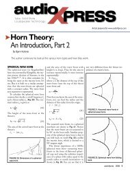
FROM STEINER FORMULAS FOR CONESTO CONCENTRATION OF INTRINSIC VOLUMESMICHAEL B. MCCOY AND JOEL A. TROPPABSTRACT. The intrinsic volumes of a convex cone are geometric functionals that return basic structural informationabout the cone. Recent research has demonstrated that conic intrinsic volumes are valuable for understanding thebehavior of random convex optimization problems. This paper develops a systematic technique for studying conicintrinsic volumes using methods from probability. At the heart of this approach is a general Steiner formula forcones. This result converts questions about the intrinsic volumes into questions about the projection of a Gaussianrandom vector onto the cone, which can then be resolved using tools from Gaussian analysis. The approach leads tonew identities and bounds for the intrinsic volumes of a cone, including a near-optimal concentration inequality.1. INTRODUCTIONIn the 1840s, Steiner developed a striking decomposition for the volume of a Euclidean expansion of acompact convex set K in R d . Steiner’s formula readsVol(K + λB d ) =d∑λ d−j · Vol(B d−j ) · V j (K ) for λ ≥ 0. (1.1)j =0The symbol B j refers to the Euclidean unit ball in R j , and + denotes the Minkowski sum. In other words,the volume of the expansion is just a polynomial whose coefficients depend on the set K . The geometricfunctionals V j that appear in (1.1) are called Euclidean intrinsic volumes [McM75]. Some of these are familiar,such as the usual volume V d , the surface area 2V d−1 , and the Euler characteristic V 0 . They can all be interpretedas measures of content that are invariant under rigid motions and isometric embedding [Sch93].In the 1940s, researchers found an analogue of the Steiner formula in spherical geometry [Her43, All48,San50]. This result expresses the size of an angular expansion of a closed convex cone C in R d .Vol { x ∈ S d−1 : dist 2 (x,C) ≤ λ } =d∑β j,d (λ) · v j (C) for λ ∈ [0,1]. (1.2)j =0We have written S d−1 for the Euclidean unit sphere in R d , and the functions β j,d : [0,1] → R + do not dependon the cone C. The geometric functionals v j that appear in (1.2) are called conic intrinsic volumes. Thesequantities serve as measures of content for a convex cone; they are invariant under rotation and embedding;and they arise in many other geometric problems. In short, the conic intrinsic volumes capture fundamentalstructural information about a convex cone [SW08].The intrinsic volumes of a closed convex cone C in R d satisfy several important identities [SW08,Thm. 6.5.5]. In particular, the numbers v 0 (C),..., v d (C) are nonnegative and sum to one, so they describe aprobability distribution on the set {0,1,2,...,d}. Thus, we can define a random variable V C by the relationsP { V C = k } = v k (C)for each k = 0,1,2,...,d.This construction invites us to use probabilistic methods to study the cone C.Recent research [ALMT13, Thm. 6.1] has determined that the random variable V C concentrates sharplyabout its mean value for every closed convex cone C. In other words, most of the intrinsic volumes of a conehave negligible size; see Figure 1.1 for a typical example. As a consequence of this phenomenon, a smallnumber of statistics of V C capture the salient information about the cone. For many purposes, we only needDate: 23 August 2013.2010 Mathematics Subject Classification. Primary: 52A22, 60D05. Secondary: 52A20.Key words and phrases. Concentration inequality; convex cone; Gaussian width; integral geometry; intrinsic volume; geometricprobability; statistical dimension; Steiner formula; variance bound.1

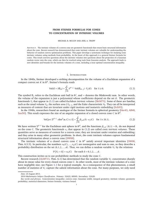
2 M. B. MCCOY AND J. A. TROPP0.0800.06–50.04–100.02–150.000 10 20 30 40 50 60–200 10 20 30 40 50 60FIGURE 1.1: The intrinsic volumes of a circular cone. These two diagrams depict the intrinsic volumes v k (C)of a circular cone C with angle π/6 in R 64 , computed using the formulas from [Ame11, Ex. 4.4.8]. The intrinsicvolume random variable V C has mean E[V C ] ≈ 16.5 and variance Var[V C ] ≈ 23.25. The tails of V C exhibit Gaussiandecay near the mean and Poisson decay farther away. [left] The intrinsic volumes v k (C) coincide with theprobability mass function of V C . [right] The logarithms log 10 (v k (C)) of the intrinsic volumes have a quadraticprofile near k = E[V C ], which is indicative of the Gaussian decay.to know the mean, the variance, and the type of tail decay. This paper develops a systematic technique forcollecting this kind of information.Our method depends on a generalization of the spherical Steiner formula (1.2). This result, Theorem 3.1,allows us to compute statistics of the intrinsic volume random variable V C by passing to a geometric randomvariable that we can study directly. The prospect for making this type of argument is dimly visible in theSteiner formula (1.2): the right-hand side can be interpreted as a moment of V C , while the left-hand sidereflects the probability that a certain geometric event occurs. Our general Steiner formula provides theflexibility we need to study a wider class of statistics.This species of argument was proposed by our collaborator Martin Lotz. In our joint paper [ALMT13], weused a laborious version of the technique to show that the intrinsic volumes concentrate. Here, we simplifyand strengthen the method to obtain new relations for the variance of V C and to improve the concentrationinequalities. Our work fits into a larger program that studies convex optimization problems with sophisticatedtools from geometry; for examples, see [VS86, VS92, Don06, BCL08, DT10, BCL10, AB11, AB12a, AB12b,MT12, ALMT13, McC13].1.1. Roadmap. Section 2 contains the definition and basic properties of the conic intrinsic volumes. Section 3states our master Steiner formula for convex cones, and it explains how to derive formulas for the size of anexpansion of a convex cone. We begin our probabilistic analysis of the intrinsic volumes in Section 4. Thismaterial includes formulas and bounds for the variance and exponential moments of the intrinsic volumerandom variable. Section 5 continues with a probabilistic treatment of the intrinsic volumes of a product cone.We provide several detailed examples of these methods in Section 6. Afterward, Section 7 summarizes somebackground material about convex cones in preparation for the proof of master Steiner formula in Section 8.2. THE INTRINSIC VOLUMES OF A CONVEX CONEWe begin with an introduction to the conic intrinsic volumes that is motivated by the treatment in [Ame11].Our presentation requires some familiarity with the geometry of convex cones. Check Section 7 for anyunexplained terms or notation; we provide cross references whenever possible.Let C d denote the family of closed convex cones in R d . To each cone of this collection, we will assign asequence of intrinsic volumes. For polyhedral cones, these functionals have a clear geometric meaning, so westart with the definition for this special case.

STEINER FORMULAS FOR CONES AND INTRINSIC VOLUMES 3Definition 2.1 (Intrinsic volumes of a polyhedral cone). Let C ∈ C d be a polyhedral cone. For k = 0,1,2,...,d,the conic intrinsic volume v k (C) is the quantityv k (C) := P { Π C (g ) lies in the relative interior of a k-dimensional face of C } .The metric projector Π C onto the cone is defined in (7.1), and the random vector g ∼ NORMAL(0,I) is drawnfrom the standard normal distribution on R d .As Section 7.5 will explain, we can equip the set C d with the conic Hausdorff metric to form a compactmetric space. The polyhedral cones form a dense subset of C d , so it is natural to use approximation to extendthe definition of the intrinsic volumes to nonpolyhedral cones.Definition 2.2 (Intrinsic volumes of a closed convex cone). Let C ∈ C d be a closed convex cone. Consider anysequence (C i ) i∈N of polyhedral cones in C d where C i → C in the conic Hausdorff metric. Definev k (C) := limi→∞v k (C i ) for k = 0,1,2,...,d. (2.1)The geometric functionals v k : C d → [0,1] are called conic intrinsic volumes.See Section 8.2 for a proof that the limit in (2.1) is well defined. The reader should be aware that thegeometric interpretation of intrinsic volumes from Definition 2.1 breaks down for general cones because thelimiting process does not preserve facial structure.The conic intrinsic volumes have some remarkable properties. Fix the ambient dimension d, and let C ∈ C dbe a closed convex cone in R d . The intrinsic volumes are...(1) Intrinsic. The intrinsic volumes do not depend on the dimension of the space R d in which the coneC is embedded. That is, for each natural number r ,{vk (C), 0 ≤ k ≤ dv k (C × {0 r }) =0, d < k ≤ d + r.(2) Volumes. Let γ d denote the standard normal measure on R d . Then v d (C) = γ d (C) and v 0 (C) = γ d (C ◦ )where C ◦ denotes the polar cone. The other intrinsic volumes, however, do not admit such a clearinterpretation.(3) Rotation invariant. For each d × d orthogonal matrix Q, we have v k (QC) = v k (C).(4) A distribution. The intrinsic volumes form a probability distribution on {0,1,2,...,d}. That is,v k (C) ≥ 0andd∑v j (C) = 1.(5) Indicators of dimension for a subspace. For any j-dimensional subspace L j ⊂ R d , we have{1, k = jv k (L j ) =0, k ≠ j.(6) Reversed under polarity. The intrinsic volumes of the polar cone C ◦ satisfyj =0v k (C ◦ ) = v d−k (C).These claims follow from Definition 2.2 using facts from Section 7 about the geometry of convex cones.Remark 2.3 (Notation for intrinsic volumes). The notation v k for the kth intrinsic volume does not specifythe ambient dimension. This convention is justified because the intrinsic volumes of a cone do not depend onthe embedding dimension.3. A GENERALIZED STEINER FORMULA FOR CONESAs we have seen, the intrinsic volumes of a cone form a probability distribution. Probabilistic methods offera powerful technique for studying the intrinsic volumes. To pursue this idea, we want access to momentsand other statistics of the sequence of intrinsic volumes. We acquire this information using a general Steinerformula for cones.

4 M. B. MCCOY AND J. A. TROPP3.1. The master Steiner formula. Let us introduce a class of Gaussian integrals. Fix a Borel measurablebivariate function f : R 2 + → R. Consider the geometric functionalϕ f : C d → R where ϕ f (C) := E [ f ( ‖Π C (g )‖ 2 , ‖Π C ◦(g )‖ 2 )] . (3.1)Throughout the paper, we reserve the letter g for a standard normal random vector whose dimension isdetermined by context, and all expectations are interpreted as Lebesgue integrals. We can develop an elegantexpansion of ϕ f in terms of the conic intrinsic volumes.Theorem 3.1 (Master Steiner formula for cones). Let f : R 2 + → R be a Borel measurable function. Then thegeometric functional ϕ f defined in (3.1) admits the expressionϕ f (C) =d∑ϕ f (L k ) · v k (C) for C ∈ C d (3.2)k=0provided that all the expectations in (3.2) are finite. Here, L k denotes a k-dimensional subspace of R d and theconic intrinsic volumes v k are introduced in Definition 2.2.The coefficients ϕ f (L k ) in the expression (3.2) have an alternative form that is convenient for computations.Let L k be an arbitrary k-dimensional subspace of R d . According to the definition (3.1) of the functional ϕ f ,ϕ f (L k ) = E [ f ( ‖Π Lk (g )‖ 2 , ‖Π Lk◦(g )‖ 2 )] .The marginal property of the standard normal vector g ensures that Π Lk (g ) and Π Lk◦(g ) are independentstandard normal vectors supported on L k and L k ◦ . Thus, ‖Π Lk (g )‖ 2 and ‖Π Lk◦(g )‖ 2 are independent chi-squarerandom variables with k and d − k degrees of freedom respectively. Note the convention that a chi-squarevariable with zero degrees of freedom is identically zero. In view of this fact, we have the following equivalentof Theorem 3.1.Corollary 3.2. Instate the hypotheses and notation of Theorem 3.1. Let { X 0 ,..., X d} be an independent sequenceof random variables where X k has the chi-square distribution with k degrees of freedom, and let { X ′ 0 ,..., X ′ d} bean independent copy of this sequence. Thenϕ f (C) =d∑E [ f ( X k, Xd−k)] ′ · vk (C) for C ∈ C d .k=0Corollary 3.2 has an appealing probabilistic consequence. For every cone C ∈ C d , the random variable‖Π C (g )‖ 2 is a mixture of chi-square random variables X 0 ,..., X d where the mixture coefficients v k (C) aredetermined solely by the cone.We outline the proof of Theorem 3.1 in Sections 7 and 8. The argument involves techniques that arealready familiar to experts. Many of the core ideas appear in McMullen’s influential paper [McM75]. Asimilar approach has been used in hyperbolic integral geometry [San80, p. 242]; see also the proof of [SW08,Thm. 6.5.1]. The only technical novelty is our method for showing that the conic intrinsic volumes arecontinuous with respect to the conic Hausdorff metric.3.2. How big is the expansion of a cone? The Euclidean Steiner formula (1.1) describes the volume of aEuclidean expansion of a compact convex set. Although it may not be obvious from the identity (3.2), themaster Steiner formula contains information about the volume of an expansion of a convex cone. This sectionexplains the connection, which justifies our decision to call Theorem 3.1 a Steiner formula.First, we argue that there is a simple expression for the Gaussian measure of a Euclidean expansion of aconvex cone.Proposition 3.3 (Gaussian Steiner formula). For each cone C ∈ C d and each number λ ≥ 0,γ d (C + λB d ) = P { dist 2 (g ,C) ≤ λ } =d∑P { X d−k ≤ λ } · v k (C) (3.3)where γ d is the standard normal measure on R d and B d is the unit ball in R d . The random variable X k followsthe chi-square distribution with k degrees of freedom.k=0

STEINER FORMULAS FOR CONES AND INTRINSIC VOLUMES 5Proof. The first identity in (3.3) is immediate. For the second, we appeal to Corollary 3.2 with the function{1, b ≤ λf (a,b) =0, otherwise.This step yields the relationP { dist 2 (g ,C) ≤ λ } = P { ‖Π C ◦(g )‖ 2 ≤ λ } =d∑E [ f ( X k , X ′ )] d∑d−k = P { X ′ d−k ≤ λ} · v k (C).k=0The first equality depends on the representation (7.3) of the distance to a cone in terms of the metric projectoronto the polar cone. The result (3.3) follows because X ′ d−k has the same distribution as X d−k.□We can also establish the spherical Steiner formula (1.2) as a consequence of Theorem 3.1 by replacing theGaussian vector g in Proposition 3.3 with a random vector θ that is uniformly distributed on the Euclideanunit sphere. This strategy leads to an expression for the proportion of the sphere subtended by an angularexpansion of the cone.Proposition 3.4 (Spherical Steiner formula). For each cone C ∈ C d and each number λ ∈ [0,1], it holds thatP { dist 2 (θ,C) ≤ λ } =k=0d∑P { B d−k,d ≤ λ } · v k (C). (3.4)k=0The random vector θ is drawn from the uniform distribution on the unit sphere S d−1 in R d , and the randomvariable B j,d follows the ( 1BETA2 j, 12 d) distribution.Proof. When λ = 1, both sides of (3.4) equal one. For λ < 1, we convert the spherical variable to a Gaussianusing the relation θ ∼ g /‖g ‖ where ∼ denotes equality of distribution. It follows thatP { dist 2 (θ,C) ≤ λ } = P { ‖Π C ◦(g )‖ 2 ≤ λ(1 − λ) −1 · ‖Π C (g )‖ 2 } .This identity depends on the representation (7.3) of the distance, the nonnegative homogeneity of the metricprojector Π C ◦, and the Pythagorean relation (7.4). Apply Corollary 3.2 with the function{1, b ≤ λ(1 − λ) −1 af (a,b) =0, otherwise.To finish, we recall the geometric interpretation [Art02] of the beta random variable: B j,d ∼ ‖Π L j(θ)‖ 2 whereL j is a j-dimensional subspace of R d .□4. PROBABILISTIC ANALYSIS OF INTRINSIC VOLUMESIn this section, we sic probabilistic methods on the conic intrinsic volumes. Our main tool is the masterSteiner formula, Theorem 3.1, which we use repeatedly to convert statements about the intrinsic volumes of acone into statements about the projection of a Gaussian vector onto the cone. We may then apply methodsfrom Gaussian analysis to study this random variable.4.1. The intrinsic volume random variable. Definitions 2.1 and 2.2 make it clear that the intrinsic volumesform a probability distribution. This observation suggests that it would be fruitful to analyze the intrinsicvolumes using techniques from probability. We begin with the key definition.Definition 4.1 (Intrinsic volume random variable). Let C ∈ C d be a closed convex cone. The intrinsic volumerandom variable V C has the distributionP { V C = k } = v k (C)for k = 0,1,2,...,d.Notice that the intrinsic volume random variable of a cone C ∈ C d and its polar have a tight relationship:P { V C ◦ = k } = v k (C ◦ ) = v d−k (C)because polarity reverses the sequence of intrinsic volumes. In other words, V C ◦ ∼ d −V C .

6 M. B. MCCOY AND J. A. TROPP4.2. The statistical dimension of a cone. The expected value of the intrinsic volume random variable V Chas a distinguished place in the theory because V C concentrates sharply about this point. In anticipation ofthis result, we glorify the expectation of V C with its own name and notation.Definition 4.2 (Statistical dimension [ALMT13, Sec. 5.3]). The statistical dimension δ(C) of a cone C ∈ C d isthe quantityd∑δ(C) := E[V C ] = k v k (C).The statistical dimension of a cone really is a measure of its dimension. In particular,k=0δ(L) = dim(L) for each subspace L ⊂ R d . (4.1)In fact, the statistical dimension is the canonical extension of the dimension of a subspace to the class ofconvex cones [ALMT13, Sec. 5.3]. By this, we mean that the statistical dimension is the only rotation invariant,continuous valuation on C d that satisfies (4.1) and that is localizable. See [SW08, p. 254 and Thm. 6.5.4] forfurther information about the unexplained technical terms.The statistical dimension interacts beautifully with the polarity operation. In particular,δ(C) + δ(C ◦ ) = E[V C ] + E[V C ◦] = E[V C ] + E[d −V C ] = d.This formula allows us to evaluate the statistical dimension of an important class of cones. A closed convexcone C is self-dual when it satisfies the identity C = −C ◦ . Examples include the nonnegative orthant, thesecond-order cone, and the cone of positive-semidefinite matrices. We haveδ(C) = 1 2 d for a self-dual cone C ∈ C d. (4.2)The statistical dimension of a cone can be expressed in terms of the projection of a normal random vectoronto the cone [ALMT13, Prop. 5.11]. The master Steiner formula gives an easy proof of this result.Proposition 4.3 (Statistical dimension). Let C ∈ C d be a closed convex cone. Thenδ(C) = E [ ‖Π C (g )‖ 2 ] .The identity in Proposition 4.3 can be used to evaluate the statistical dimension for many cones of interest.See [ALMT13, Sec. 4] for details and examples.Proof. The master Steiner formula, Corollary 3.2, with function f (a,b) = a states thatE [ ‖Π C (g )‖ 2 ] d∑= E [ ] d∑X k · vk (C) = k v k (C) = δ(C).Indeed, a chi-square variable X k with k degrees of freedom has expectation k.k=04.3. The variance of the intrinsic volumes. The variance of the intrinsic volume random variable tells ushow tightly the intrinsic volumes cluster around their mean value. We can find an explicit expression for thevariance in terms of the projection of a Gaussian vector onto the cone.Proposition 4.4 (Variance of the intrinsic volumes). Let C ∈ C d be a closed convex cone. Thenk=0Var[V C ] = Var [ ‖Π C (g )‖ 2 ] − 2δ(C) (4.3)= Var [ ‖Π C ◦(g )‖ 2 ] − 2δ(C ◦ ) = Var[V C ◦]. (4.4)Proposition 4.4 leads to exact formulas for the variance of the intrinsic volume sequence in severalinteresting cases; Section 6 contains some worked examples.Proof. By definition, the variance satisfiesVar[V C ] = E [ V 2 C]−(E[VC ] ) 2 = E[V2C]− δ(C) 2 .To obtain the expectation of V 2 C, we invoke the master Steiner formula, Corollary 3.2, with the functionf (a,b) = a 2 to obtainE [ ‖Π C (g )‖ 4 ] d∑= E [ X 2 ] d∑d∑k · vk (C) = k 2 v k (C) + 2 k v k (C) = E [ V 2 ]C + 2δ(C).k=0k=0k=0□

STEINER FORMULAS FOR CONES AND INTRINSIC VOLUMES 7Indeed, the raw second moment of a chi-square random variable X k with k degrees of freedom equals k 2 + 2k.Combine these two displays to reachVar[V C ] = E [ ‖Π C (g )‖ 4 ] − δ(C) 2 − 2δ(C) = E [ ‖Π C (g )‖ 4 ] − ( E [ ‖Π C (g )‖ 2 ]) 2 − 2δ(C)where the second identity follows from Proposition 4.3. Identify the variance of ‖Π C (g )‖ 2 to complete theproof of (4.3). To establish (4.4), note that Var[V C ] = Var[d − V C ] = Var[V C ◦], and then apply (4.3) to therandom variable V C ◦.□4.4. A bound for the variance of the intrinsic volumes. Proposition 4.4 also allows us to produce a generalbound on the variance of the intrinsic volumes of a cone.Theorem 4.5 (Variance bound for intrinsic volumes). Let C ∈ C d be a closed convex cone. ThenThe operator ∧ returns the minimum of two numbers.Var[V C ] ≤ 2 ( δ(C) ∧ δ(C ◦ ) ) .The example in Section 6.3 demonstrates that the constant two in (4.5) cannot be reduced.Proof. To bound the variance of V C , we plan to invoke the Gaussian Poincaré inequality [Bog98, Thm. 1.6.4]to control the variance of ‖Π C (g )‖ 2 . This inequality states thatVar[H(g )] ≤ E [ ‖∇H(g )‖ 2 ] .for any function H : R d → R whose gradient is square-integrable with respect to the standard normal measure.We apply this result to the functionH(x) = ‖Π C (x)‖ 2 with ‖∇H(x)‖ 2 = 4‖Π C (x)‖ 2 .The gradient calculation is justified by (7.5). We determine thatVar [ ‖Π C (g )‖ 2 ] ≤ 4E [ ‖Π C (g )‖ 2 ] = 4δ(C)where the second identity follows from Proposition 4.3. Introduce this inequality into (4.3) to see thatVar[V C ] ≤ 2δ(C). We can apply the same argument to see thatVar [ ‖Π C ◦(g )‖ 2 ] ≤ 4δ(C ◦ ).Substitute this bound into (4.4) to conclude that Var[V C ] ≤ 2δ(C ◦ ).In principle, a random variable taking values in {0,1,2,...,d} can have variance larger than d 2 /3—considerthe uniform random variable. In contrast, Theorem 4.5 tells us that the variance of the intrinsic volumerandom variable V C cannot exceed d for any cone C. This observation has consequences for the tail behaviorof V C . Indeed, Chebyshev’s inequality implies that{P |V C − δ(C)| > λ √ }δ(C)≤ Var[V C ]λ 2 δ(C) ≤ 2 λ 2 .That is, most of the mass of V C is located near the statistical dimension.4.5. Exponential moments of the intrinsic volumes. In the previous section, we discovered that theintrinsic volume random variable V C is often close to its mean value. This observation suggests that V Cmight exhibit stronger concentration. A standard method for proving concentration inequalities for a randomvariable is to calculate its exponential moments. The master Steiner formula allows us to accomplish this task.Proposition 4.6 (Exponential moments of the intrinsic volumes). Let C ∈ C d be a closed convex cone. For eachparameter ζ ∈ R,Ee ζV C= Ee ξ‖Π C (g )‖ 2 where ξ = 1 2(1 − e−2ζ ) .Proof. Fix a number ξ < 1 2 . With the choice f (a,b) = eξa , Corollary 3.2 shows thatd∑Ee ξ‖Π C (g )‖ 2 [ ] d∑d∑= EeξX k · vk (C) = (1 − 2ξ) −k/2 v k (C) = e ζk v k (C) = Ee ζV C.k=0k=0We have used the familiar formula for the exponential moments of a chi-square random variable X k with kdegrees of freedom. The penultimate identity follows from the change of variables ζ = − 1 2log(1 − 2ξ), whichestablishes a bijection between ξ < 1 2and ζ ∈ R.□k=0□

8 M. B. MCCOY AND J. A. TROPPRemark 4.7 (Conic Wills functional). Proposition 4.6 leads to a geometric description of the generatingfunction of the intrinsic volumes:( 1 − λW C (λ) := λ d 2) d∑Eexp · dist 2 (g ,C) = λ k v k (C) for λ > 0. (4.5)2To see why this is true, use the representation (7.3) of the distance, and apply Proposition 4.6 with ζ = −logλto confirm that( 1 − λW C (λ) = λ d 2)Eexp · ‖Π C ◦(g )‖ 2 = λ d ∑ d d∑λ −k v k (C ◦ ) = λ k v k (C).2We have applied the fact that polarity reverses intrinsic volumes to reindex the sum. The function W C can beviewed as a conic analog of the Wills functional [Wil73] from Euclidean geometry.4.6. A bound for the exponential moments of the intrinsic volumes. Proposition 4.6 allows us to obtainan excellent bound for the exponential moments of V C . In the next section, we use this result to developconcentration inequalities for the intrinsic volumes.Theorem 4.8 (Exponential moment bound for intrinsic volumes). Let C ∈ C d be a closed convex cone. For eachparameter ζ ∈ R,()Ee ζ(V C −δ(C)) e 2ζ − 2ζ − 1≤ exp· δ(C) , and (4.6)2()Ee ζ(V C −δ(C)) e −2ζ + 2ζ − 1≤ exp· δ(C ◦ ) . (4.7)2The major technical challenge is to bound the exponential moments of the random variable ‖Π C (g )‖ 2 .The following lemma provides a sharp estimate for the exponential moments. It improves on an earlierresult [ALMT13, Sublem. D.3].Lemma 4.9. Let C ∈ C d be a closed convex cone. For each parameter ξ < 1 2 ,(Ee ξ(‖Π C (g )‖ 2 2ξ −δ(C)) 2 )δ(C)≤ exp .1 − 2ξProof. Define the zero-mean random variablek=0k=0Z := ‖Π C (g )‖ 2 − δ(C).Introduce the moment generating function m(ξ) := Ee ξZ . Our aim is to bound m(ξ). Before we begin, it ishelpful to note a few properties of the moment generating function. First, the derivative m ′ (ξ) = E[Z e ξZ ] wheneverξ < 1 2 . By direct calculation, logm(0) = 0. Furthermore, l’Hôpital’s rule shows that lim ξ→0 ξ −1 logm(ξ) = 0because the random variable Z has zero mean.The argument is based on the Gaussian logarithmic Sobolev inequality [Bog98, Thm. 1.6.1]. One versionof this result states thatE [ H(g ) · e H(g )] − E [ e H(g )] log E [ e H(g )] ≤ 1 2 E[ ‖∇H(g )‖ 2 · e H(g )] (4.8)for any differentiable function H : R d → R such that the expectations in (4.8) are finite. We apply this result tothe functionH(x) = ξ [ ‖Π C (x)‖ 2 − δ(C) ] with ‖∇H(x)‖ = 4ξ 2 ‖Π C (x)‖ 2 .The gradient calculation is justified by (7.5). Notice thatH(g ) = ξZ and ‖∇H(g )‖ 2 = 4ξ 2 (Z + δ(C)).Therefore, the logarithmic Sobolev inequality (4.8) delivers the relationξ · E [ Z e ξZ ] − E [ e ξZ ] log E [ e ξZ ] ≤ 2ξ 2 · E [ Z e ξZ ] + 2ξ 2 δ(C) · E [ e ξZ ] for ξ < 1 2 .We can rewrite the last display as a differential inequality for the moment generating function:ξm ′ (ξ) − m(ξ)logm(ξ) ≤ 2ξ 2 m ′ (ξ) + 2δ(C) · ξ 2 m(ξ) for ξ < 1 2 . (4.9)The requirement on ξ is necessary and sufficient to ensure that m(ξ) and m ′ (ξ) are finite. To complete theproof, we just need to solve this differential inequality.k=0

STEINER FORMULAS FOR CONES AND INTRINSIC VOLUMES 9We follow the argument from [BLM03, Thm. 5]. Divide the inequality (4.9) by the positive number ξ 2 m(ξ)to reach1ξ · m′ (ξ)m(ξ) − 1 ξ 2 logm(ξ) ≤ 2 · m′ (ξ)m(ξ) + 2δ(C) for ξ ∈ (−∞,0) ∪ ( 0, 1 )2 .The left- and right-hand sides of this relation are exactly integrable:[ ]d 1ds s logm(s) ≤ 2 · d [ ]logm(s) + 2δ(C) · s for s ∈ (−∞,0) ∪ ( 0, 1 )ds2 . (4.10)To continue, we first consider the case 0 < ξ < 1 2. Integrate the inequality (4.10) over the interval s ∈ [0,ξ]using the boundary conditions logm(0) = 0 and lim ξ→0 ξ −1 logm(ξ) = 0. This step yields1ξ logm(ξ) ≤ 2logm(ξ) + 2δ(C) · ξ for 0 < ξ < 1 2 .Solve this relation for the moment generating function m to obtain the bound( 2ξ 2 )δ(C)m(ξ) ≤ expfor 0 ≤ ξ < 11 − 2ξ2 . (4.11)The boundary case ξ = 0 follows from a direct calculation. Next, we address the situation where ξ < 0.Integrating (4.10) over the interval [ξ,0], we find that− 1 logm(ξ) ≤ −2logm(ξ) − 2δ(C) · ξ for ξ < 0.ξSolve this inequality for m to see that the bound (4.11) also holds in the range ξ < 0. This observationcompletes the proof.□With Lemma 4.9 at hand, we quickly reach Theorem 4.8.Proof of Theorem 4.8. We begin with the statement from Proposition 4.6. Adding and subtracting multiples ofδ(C) in the exponent, we obtain the relationEe ζ(V C −δ(C)) = e (ξ−ζ)δ(C) · Ee ξ(‖Π C (g )‖ 2 −δ(C)) .where ξ = 1 (2 1 − e−2ζ ) < 1 2. Lemma 4.9 controls the moment generating function on the right-hand side:(Ee ζ(V C 2ξ −δ(C)) ≤ e (ξ−ζ)δ(C) 2 )δ(C)· exp .1 − 2ξBy a marvelous coincidence, the terms in the exponent collapse into a compact form:ξ − ζ +2ξ21 − 2ξ = e2ζ − 2ζ − 1.2Combine the last two displays to finish the proof of (4.6). To obtain the second formula (4.7), note thatEe ζ(V C −δ(C)) = Ee (−ζ)(V C ◦ −δ(C ◦ ))because V C ∼ d −V C ◦ and δ(C) = d − δ(C ◦ ). Now apply (4.6) to the right-hand side.□4.7. Concentration of intrinsic volumes. The exponential moment bound from Theorem 4.8 allows us toobtain concentration results for the sequence of intrinsic volumes of a convex cone. The following corollaryprovides Bennett-type inequalities for the intrinsic volume random variable.Corollary 4.10 (Concentration of the intrinsic volume random variable). Let C ∈ C d be a closed convex cone.For each λ ≥ 0, the intrinsic volume random variable V C satisfies the upper tail boundP { V C − δ(C) ≥ λ } ≤ exp(− 1 { ( ) ( )})λ−λ2 max δ(C) · ψ , δ(C ◦ ) · ψδ(C)δ(C ◦ (4.12))and the lower tail boundP { V C − δ(C) ≤ −λ } ≤ exp(− 1 { ( ) (−λ2 max δ(C) · ψ , δ(C ◦ ) · ψδ(C)The function ψ(u) := (1 + u)log(1 + u) − u for u ≥ −1 while ψ(u) = ∞ for u < −1.λδ(C ◦ ))}). (4.13)

10 M. B. MCCOY AND J. A. TROPPProof. The argument, based on the Laplace transform method, is standard. For any ζ > 0,P { V C − δ(C) ≥ λ } ()≤ e −ζλ · Ee ζ(V C −δ(C)) ≤ e −ζλ e 2ζ − 2ζ − 1· exp· δ(C)2where we have applied the exponential moment bound (4.6) from Theorem 4.8. Minimize the right-hand sideover ζ > 0 to obtain the first branch of the maximum in (4.12). The second exponential moment bound (4.7)leads to the second branch of the maximum in (4.12). The lower tail bound (4.13) follows from the sameconsiderations. For more details about this type of proof, see [BLM13, Sec. 2.7].□To understand the content of Corollary 4.10, it helps to make some further estimates. Comparing Taylorseries, we find that ψ(u) ≥ u 2 /(2 + 2u/3). This observation leads to a weaker form of the tail bounds (4.12)and (4.13). For λ ≥ 0,P { V C − δ(C) ≥ λ } (−λ 2 )/4≤ exp(δ(C) + λ/3) ∧ (δ(C ◦ ) − λ/3)P { V C − δ(C) ≤ −λ } (−λ 2 /4≤ exp(δ(C) − λ/3) ∧ (δ(C ◦ ) + λ/3)This pair of inequalities reflects the fact that the left tail of V C exhibits faster decay than the right tail when thestatistical dimension δ(C) is small; the tail behavior is reversed when δ(C) is close to the ambient dimension.For practical purposes, it seems better to combine these estimates into a single bound:P { |V C − δ(C)| ≥ λ } (−λ 2 )/4≤ 2exp(δ(C) ∧ δ(C ◦ for λ ≥ 0. (4.14))) + λ/3This tail bound indicates that V C looks somewhat like a Gaussian variable with mean δ(C) and variance2(δ(C) ∧ δ(C ◦ )) or less. This claim is consistent with Theorem 4.5. The result (4.14) improves over [ALMT13,Thm. 6.1], and we will see an example in Section 6.3 that saturates the bound.Our analysis suggests that the intrinsic volume sequence of a convex cone C cannot exhibit very complicatedbehavior. Indeed, the statistical dimension δ(C) already tells us almost everything there is to know. Theonly large intrinsic volumes v k (C) are those where the index k is in the range δ(C) ± const · δ(C)∧ δ(C ◦ ).The consequence of this result for conic integral geometry is that a cone with statistical dimension δ(C)behaves essentially like a subspace with dimension [δ(C)]. See [ALMT13] for more support of this point andits consequences for convex optimization.).5. INTRINSIC VOLUMES OF PRODUCT CONESSuppose that C 1 ∈ C d1 and C 2 ∈ C d2 are closed convex cones. We can form another closed convex cone bytaking their direct product:C 1 ×C 2 := { (x 1 , x 2 ) ∈ R d 1+d 2: x 1 ∈ C 1 and x 2 ∈ C 2}∈ Cd1 +d 2.The probabilistic methods of the last section are well suited to the analysis of a product cone. In this section,we compute the intrinsic volumes of a product cone using these techniques. Then we identify the mean,variance, and concentration behavior of the intrinsic volume random variable of a product cone.5.1. The product rule for intrinsic volumes. The intrinsic volumes of the product cone can be derived fromthe intrinsic volumes of the two factors.Corollary 5.1 (Product rule for intrinsic volumes). Let C 1 ∈ C d1 and C 2 ∈ C d2 be closed convex cones. Theintrinsic volumes of the product cone C 1 ×C 2 satisfyv k (C 1 ×C 2 ) =∑v i (C 1 ) · v j (C 2 ) for k = 0,1,2,...,d 1 + d 2 . (5.1)i+j =kWe present a short proof of Corollary 5.1 based on the conic Wills functional (4.5). This approach echoesHadwiger’s method [Had75] for computing the Euclidean intrinsic volumes of a product of convex sets.

STEINER FORMULAS FOR CONES AND INTRINSIC VOLUMES 11Proof. Let g 1 ∈ R d 1and g 2 ∈ R d 2be independent standard normal vectors. The direct product (g 1 , g 2 ) is astandard normal vector on R d 1+d 2. For each λ > 0, the definition (4.5) of the Wills functional gives(W C1 ×C 2(λ) = λ d 1+d 2 1 − λ2E exp · dist 2 ( ) )(g 1 , g 2 ),C 1 ×C 22(= λ d 1 1 − λ2) (E exp · dist 2 (g 1 ,C 1 ) · λ d 2 1 − λ2)E exp · dist 2 (g 2 ,C 2 ) = W C1 (λ) ·W C2 (λ).22The second identity follows from the fact that the squared distance to a product cone equals the sum of thesquared distances to the factors; we have also invoked the independence of the standard normal vectors tosplit the expectation. Applying the relation (4.5) twice, we find thatW C1 ×C 2(λ) = W C1 (λ) ·W C2 (λ) =But (4.5) also shows that(d1∑λ i v i (C 1 )i=0)∑λ j v j (C 2 ))(d2j =0d 1 ∑+d 2W C1 ×C 2(λ) = λ k v k (C 1 ×C 2 ).k=0∑d 1 +d 2=k=0Comparing coefficients in these two polynomials, we arrive at the relation (5.1).λ k∑i+j =kv i (C 1 ) · v j (C 2 ).5.2. Concentration of the intrinsic volumes of a product cone. We can employ the probabilistic techniquesfrom Section 4 to collect information about the intrinsic volumes of a product cone. Let C 1 ∈ C d1 and C 2 ∈ C d2be two cones, and consider independent random variables V C1 and V C2 whose distributions are given by theintrinsic volumes of C 1 and C 2 . In view of Corollary 5.1,v k (C 1 ×C 2 ) =∑v i (C 1 ) · v j (C 2 ) = P { V C1 +V C2 = k } for k = 0,1,2,...,d 1 + d 2 .i+j =kIn other words, the intrinsic volume random variable V C1 ×C 2of the product cone has the distributionV C1 ×C 2∼ V C1 +V C2 . (5.2)This observation allows us to compute the statistical dimension of the product cone:δ(C 1 ×C 2 ) = E [ V C1 ×C 2]= δ(C1 ) + δ(C 2 ). (5.3)Of course, we can also derive (5.3) directly from Proposition 4.3. A more interesting consequence is thefollowing expression for the variance of the intrinsic volumes:Var [ V C1 ×C 2]= Var[VC1 ] + Var[V C2 ] ≤ 2 [( δ(C 1 ) ∧ δ(C ◦ 1 )) + ( δ(C 2 ) ∧ δ(C ◦ 2 ))] . (5.4)The inequality follows from Theorem 4.5. With some additional effort, we can develop a concentration resultfor the intrinsic volumes of a product cone that matches the variance bound (5.4).Corollary 5.2 (Concentration of intrinsic volumes for a product cone). Let C 1 ∈ C d1 and C 2 ∈ C d2 be closedconvex cones. For each λ ≥ 0,P {∣ ∣ VC1 ×C 2− δ(C 1 ×C 2 ) ∣ (} −λ 2 )/4≥ λ ≤ 2 expσ 2 where σ 2 := ( δ(C 1 ) ∧ δ(C1 ◦ + λ/3)) + ( δ(C 2 ) ∧ δ(C2 ◦ )) .This represents a significant improvement over the simple tail bound from [ALMT13, Lem. 7.2]. A similarresult holds for any finite product C 1 × ··· ×C r of closed convex cones.Proof. First, recall the numerical inequalitye 2ζ − 2ζ − 1≤2 1 − 2|ζ|/3ζ 2for |ζ| < 3 2 .This estimate allows us to package the two exponential moment bounds from Theorem 4.8 as(Ee ζ(V C ζ −δ(C)) 2 (δ(C) ∧ δ(C ◦ )))≤ expfor |ζ| < 31 − 2|ζ|/32 .Applying this bound twice, we learn that the exponential moments of the random variable V C1 ×C 2satisfy(Ee ζ(V C 1 ×C 2 −δ(C 1 ×C 2 )) = Ee ζ(V C 1 −δ(C 1 )) · Ee ζ(V C 2 −δ(C 2 )) ζ 2 σ 2 )≤ exp.1 − 2|ζ|/3□

12 M. B. MCCOY AND J. A. TROPPThe first relation follows from the distributional identity (5.2) and the statistical dimension calculation (5.3).The Laplace transform method delivers{ (e −ζλ ζ 2 σ 2· expP { V C1 ×C 2− δ(C 1 ×C 2 ) ≥ λ } ≤ infζ>01 − 2|ζ|/3)} ( −λ 2 )/4≤ expσ 2 .+ λ/3We have chosen ζ = λ/(2σ 2 + 2λ/3) to reach the second inequality. We obtain the lower tail bound from thesame argument.□6. EXAMPLESIn this section, we demonstrate the vigor of the ideas from Section 4 by applying them to some concreteexamples. The probabilistic viewpoint provides new insights, and it enables us to complete some difficultcalculations with minimal effort.6.1. The nonnegative orthant. As a warmup, we begin with an example where it is easy to compute theintrinsic volumes directly. The nonnegative orthant R d + is the polyhedral coneR d + := { x ∈ R d : x i ≥ 0 for i = 1,...,d. } .The nonnegative orthant is self-dual, which immediately delivers several results. For typographical felicity, weabbreviate C = R d + . Applying the identity (4.2) and Theorem 4.5, we find thatThe tail bound (4.14) specializes toδ(C) = E [ V C]=12 d and Var[V C ] ≤ 2δ(C) = d.P {∣ ∣ VC − 1 2 d∣ ∣ ≥ λ}≤ 2 exp(−λ 22d + 4λ/3These estimates already provide a significant amount of information about the intrinsic volumes of the orthant.How well do these bounds describe the actual behavior of the intrinsic volumes? Appealing directly toDefinition 2.1, we can check that V C ∼ BINOMIAL ( d, 1 2) . Therefore,E[V C ] = 1 2 d and Var[V C ] = 1 4 d.Furthermore, the binomial random variable satisfies a sharp tail bound of the formP {∣ (∣ VC − 1 2 d∣ }∣ −2λ2)≥ λ ≤ 2 exp .dWe discover that our general results overestimate the variance of V C by a factor of four, but they do capturethe subgaussian decay of the intrinsic volumes.6.2. The cone of positive-semidefinite matrices. Our approach to intrinsic volume calculations is mostvaluable when there is no explicit formula for the intrinsic volumes, or the expressions are too complicated toevaluate easily. For a challenge of this type, let us consider the cone of real positive-semidefinite matrices. Wecan compute the mean and variance of the intrinsic volume sequence of this cone by combining our methodswith established results from random matrix theory.The cone S n + consists of all n × n positive-semidefinite (psd) matrices:S n + := { X ∈ R n×nsym : uT X u ≥ 0 for all u ∈ R n}where R n×nsym consists of n × n symmetric matrices. This vector space has dimension d = n(n + 1)/2. The psdcone is self-dual with respect to R n×nsym , so the expression (4.2) shows that the statistical dimensionδ(S n n(n + 1)+ ) = .4As with the nonnegative orthant, we immediately obtain bounds on the variance and concentration inequalitiesfor the intrinsic volumes.We will use Proposition 4.4 to compute the variance of the sequence of intrinsic volumes when n is large.Let us abbreviate C = S n + . The intrinsic volumes do not depend on the embedding dimension of the cone, sothere is no harm in treating the cone as a subset of the linear space R n×n of square matrices. To compute the).

STEINER FORMULAS FOR CONES AND INTRINSIC VOLUMES 13metric projection of a matrix X onto the cone C, we first extract the symmetric part of the matrix and thencompute the positive part [Bha97, p. 99] of the Jordan decomposition:It follows thatΠ C (X ) = Π C( 12 (X + X T ) ) = 1 2 (X + X T ) + .‖Π C (X )‖ 2 F = 1 ∥ (4X + X T ) ∥ 2+ F = 1 4 tr[( X + X T ) 2+].Let G ∈ R n×n be a matrix with independent standard normal entries. Then the matrix W n = 2 −1/2( G +G T ) ∈ R n×nsymis a member of the Gaussian orthogonal ensemble (GOE). We have‖Π C (G)‖ 2 F = 1 2 tr[ (W n ) 2 +].To invoke Proposition 4.4, we must compute the variance of this quantity.Our method is to renormalize the matrix and invoke asymptotic results for the GOE. Introduce the functionh(s) := (s) 2 + = max{s,0}2 . ThenVar [ ‖Π C (G)‖ 2 ] [ nF = Var2 · tr[( n −1/2 ) 2 ] ]W n += n24 · Var[ trh ( n −1/2 )]W n .In the limit as n → ∞, the variance of the trace can be expressed in terms of an integral against a kernelassociated with the GOE [BS10, Thm. 9.2].Var [ trh ( n −1/2 W n)]→∫ 2−2∫ 2−2h ′ (s)h ′ (t) · ρ GOE (s, t)ds dtwhere the kernel takes the form(ρ GOE (s, t) = 12π 2 log 4 − st + √ )(4 − s 2 )(4 − t 2 )4 − st − √ .(4 − s 2 )(4 − t 2 )With the assistance of a computer algebra system, we determine that the double integral equals 1 + 16/π 2 .Therefore,Var [ ‖Π C (G)‖ 2 ] n 2 (F = 1 + 16 )4 π 2 + o(n 2 ) as n → ∞.Proposition 4.4 yieldsIn particular,Var[V C ] = Var [ ‖Π C (G)‖ 2 ] n 2F − 2δ(C) =4Var[V C ]δ(C)→ 16 − 1 as n → ∞.π2 ( 16π 2 − 1 )+ o(n 2 ) as n → ∞.This ratio measures how much the intrinsic volumes are spread out relative to the size of the cone.As a point of comparison, Amelunxen & Bürgisser have computed the intrinsic volumes of the psd coneexactly using methods from differential geometry [AB12b, Thm. 3.5]. The expressions, involving Mehtaintegrals, can be evaluated for low-dimensional cones, but they have resisted asymptotic analysis.6.3. Circular cones. A circular cone C in R d with angle 0 ≤ α ≤ π/2 takes the formC = Circ d (α) := { x ∈ R d : x 1 ≥ ‖x‖cos(α) } .In particular, this family includes the second-order cone L d := Circ d (π/4). Second-order cones are also knownas Lorentz cones, and they are self-dual.With some effort, it is possible to work out the intrinsic volumes of a circular cone [Ame11, Ex. 4.4.8].Instead, we apply our techniques to compute the mean and variance of the intrinsic volume random variable.This calculation demonstrates that circular cones with a small angle saturate the variance bound fromTheorem 4.5. Afterward, we sketch an argument that small circular cones also saturate the upper tail boundfrom Corollary 4.10.

14 M. B. MCCOY AND J. A. TROPP6.3.1. Mean and variance calculations. Fix an angle α ∈ (0,π/2). We consider the circular cone C := Circ d (α)where the dimension d is large. For each unit vector u ∈ R d , elementary trigonometry shows that⎧⎪⎨ 1, β ∈ [0,α)‖Π C (u)‖ 2 = H(arccos(u 1 )) where H(β) := cos⎪⎩2 (β − α), β ∈ [α,α + π/2]0, β ∈ (α + π/2,π].Recall the polar decomposition g = R · θ where R and θ are independent, R 2 is a chi-square random variablewith d degrees of freedom, and θ is uniformly distributed on the sphere. With this notation,‖Π C (g )‖ 2 = R 2 · H ( arccos(θ 1 ) ) . (6.1)This expression allows us to evaluate the moments of ‖Π C (g )‖ 2 quickly.We begin with the statistical dimension. Combine Proposition 4.3 with the expression (6.1) and integratein polar coordinates to reachδ(C) = d ∫ πH(β)sin d−2 (β)dβ where κ d :=κ d0∫ π0sin d−2 (β)dβ.A more detailed version of this calculation appears in [McC13, Prop. 6.8]. The function β → sin d−2 (β) peakssharply around π/2, so it does little harm to replace H by the function ˜H(β) = cos 2 (β − α). Computing thissimpler integral, we obtain a closed-form expression plus a remainder term:δ(C) = d sin 2 (α) + cos(2α) + ε 1 (α,d). (6.2)We assert that the remainder term is exponentially small as a function of the dimension:√ (π|ε 1 (α,d)| 0.(α)By considering a sufficiently small angle α, we can find a circular cone C = Circ d (α) for which Var[V C ] isarbitrarily close to 2δ(C). In conclusion, we cannot improve the constant two in the variance bound fromTheorem 4.5.

STEINER FORMULAS FOR CONES AND INTRINSIC VOLUMES 156.3.2. Tail behavior. Circular cones also exhibit tail behavior that matches the predictions of Corollary 4.10exactly. It takes some technical effort to establish this claim in detail, so we limit ourselves to a sketch of theargument. These ideas are drawn from [ALMT13, Sec. 6.2].Fix an angle 0 < α ≪ π 2 , and abbreviate q = sin2 (α). Consider the circular cone C = Circ d (α) where thedimension takes the form d = 2(n +1) where n is a large integer. In particular, the formula (6.2) shows that thestatistical dimension δ(C) ≈ d sin 2 (α) ≈ 2nq. It can be established that the odd intrinsic volumes of C follow abinomial distribution [Ame11, Ex. 4.4.8]:2 v 2k+1 (C) = P { Y = k} where Y = Y n ∼ BINOMIAL(n, q).As a consequence of the Gauss–Bonnet Theorem [SW08, Thm. 6.5.5], there is an interlacing result [ALMT13,Prop. 5.6] for the upper tail of V C .P { Y ≥ k } ≤ P { V C ≥ 2k } ≤ P { Y ≥ k − 1 } .Thus, accurate probability bounds for V C follow from bounds for the binomial random variable Y .Our tail inequality, Corollary 4.10, predicts that V C has subgaussian behavior for moderate deviations. Tosee that circular cones actually display this behavior, we turn to the classical limits for the binomial randomvariable Y n . The Laplace–de Moivre central limit theorem states thatP { Y n − nq ≥ t √ nq(1 − q) } → 1 − Φ(t)as n → ∞ with q fixed.Here, Φ denotes the distribution function of a standard normal variable. When q is small and n is large, wecan invoke the approximation δ(C) ≈ 2nq and a tail bound for the normal distribution to obtainP { V C − δ(C) ≥ λ √ δ(C) } ≈ P { V C − 2nq ≥ λ √ 2nq(1 − q) } ≈ P { Y n − nq ≥ (2 −1/2 λ) √ nq(1 − q) } ≈ e −λ2 /4 .This expression matches the behavior expressed in the weaker tail bound (4.14). In other words, we see thatthe intrinsic volumes of a small circular cone have subgaussian concentration for moderate deviations, withvariance approximately 2δ(C).Corollary 4.10 also predicts that V C has Poisson tails for very large deviations. Vanishingly small circularcones display this behavior. Suppose that q = q n = b/n for a large constant b. The approximation δ(C) ≈ 2band Chernoff’s bound for the tail of a binomial random variable together giveP { V C − δ(C) ≥ λδ(C) } ≈ P { V C − 2b ≥ 2λb } ≈ P { Y n − b ≥ λb } ≈ e b (λ−(1+λ)log(1+λ)) .After a change of variables, this formula coincides with the tail bound (4.6). The Chernoff bound is quiteaccurate in this regime, so we see that (4.6) is saturated by vanishingly small circular cones in high dimensions.6.4. Summary of calculations. We conclude this section with an overview of the statistical dimension andvariance calculations. See Table 6.1 for this material. Observe that the ratio of the variance Var[V C ] to thestatistical dimension δ(C) can range from zero to two. A subspace L k with dimension k shows that the lowerbound is achievable across the entire range of statistical dimensions. The circular cones Circ d (α) show thatthe upper bound is saturated by cones whose statistical dimension is small. Amelunxen has conjectured thatsomewhat tighter bounds are possible when δ(C) ≈ 1 2d, but this remains to be established.7. BACKGROUND ON CONIC GEOMETRYThis section summarizes the foundational material that we require to establish the master Steiner formula.We provide sketches or references in lieu of proofs to keep the presentation lean. Most of the material here isdrawn from the books [Roc70, RW98, Bar02, SW08].7.1. Basics. We work in the Euclidean space R d . This space is equipped with the Euclidean inner product〈·, ·〉, the associated norm ‖·‖, and the norm topology. We write 0 or 0 d for the origin of R d .The linear hull lin(K ) of a convex set K ⊂ R d is the intersection of all subspaces that contain K . The relativeinterior relint(K ) is the interior with respect to the relative topology induced by R d on the linear hull lin(K ).We define the distance function dist 2 (x,K ) := inf { ‖x − y‖ 2 : y ∈ K } .We write P for the probability of an event and E for the expectation operator. The symbol ∼ denotesequality of distribution. We reserve the letter g for a standard normal vector, and θ denotes a vector uniformlydistributed on the sphere. The dimensions are determined by context.

16 M. B. MCCOY AND J. A. TROPPTABLE 6.1: Statistical dimension and variance calculations. This table lists the statistical dimension δ(C) andthe variance Var[V C ] for several families of convex cones. The last column displays the limiting ratio Var[V C ]/δ(C)as the dimensional parameter tends to infinity.Cone Notation Mean δ(C) Variance Var[V C ] Limit of Var[V C ]/δ(C)Subspace L k k 0 0Nonnegative orthant R d +Real positive-semidefinite cone S n +12 d 14 d 1214 n(n + 1) ≈ ( 4− 1 π 2 4)n2 16π 2 − 1Second-order cone L d 1 2 d ≈ 1 2(d − 2) 1Circular cone Circ d (α) ≈ d sin 2 (α) ≈ 1 2 (d − 2)sin2 (2α) 2cos 2 (α)Upper bound (Theorem 4.5) 27.2. Convex cones. A convex cone C is a nonempty subset of R d that satisfiesτ · (x + y) ∈ C for all τ > 0 and x, y ∈ C.We designate the family C d of all closed convex cones in R d . A cone C is polyhedral if it can be expressed asthe intersection of a finite number of halfspaces:N⋂ {C = x ∈ R d : 〈u i , x〉 ≥ 0 } for some u i ∈ R d .i=1For each cone C ∈ C d , we define the polar cone C ◦ ∈ C d via the formulaC ◦ := { u ∈ R d : 〈u, x〉 ≤ 0 for all x ∈ C } .The polar of a polyhedral cone is always polyhedral.A closed convex cone and its polar induce an orthogonal decomposition of R d . To state this wonderful fact,we introduce the metric projector Π C onto a cone C ∈ C d .Π C : R d → C where Π C (x) := arg min { ‖x − y‖ 2 : y ∈ C } . (7.1)Note that the metric projector onto a convex cone is a nonnegative homogeneous function. Given a coneC ∈ C d , every point x ∈ R d can be expressed as an orthogonal sum of the typex = Π C (x) + Π C ◦(x) where Π C (x) ⊥ Π C ◦(x). (7.2)We often use the consequence‖Π C ◦(x)‖ 2 = dist 2 (x,C). (7.3)Another outcome is the Pythagorean relation‖x‖ 2 = ‖Π C (x)‖ 2 + ‖Π C ◦(x)‖ 2 . (7.4)See Rockafellar [Roc70, pp. 338–341] for more information about this construction. Finally, we mention thatthe squared norm of the metric projection is a differentiable function:This result follows from [RW98, Thm. 2.26].∇‖Π C (x)‖ 2 = 2Π C (x) for all x ∈ R d . (7.5)7.3. The tiling induced by a polyhedral cone. Let C be a polyhedral cone. A face F (u) of C with outwardnormal u takes the formF (u) := { x ∈ C : 〈u, x〉 = sup y∈C 〈u, y〉 } .The face F (u) is nonempty if and only if u ∈ C ◦ ; otherwise, the supremum is infinite. The dimension of a faceF is the dimension of its linear hull lin(F ). The polar of a polyhedral cone is always a polyhedral cone, andthe outward normals of a face F of the cone C comprise a face N F of the polar cone C ◦ called the normal face:N F := lin(F ) ◦ ∩C ◦ .

STEINER FORMULAS FOR CONES AND INTRINSIC VOLUMES 17Each polyhedral cone C induces a tiling of R d as an orthogonal sum of the faces of C and the normal facesof C ◦ . The following statement of this claim amplifies an observation of McMullen [McM75, Lem. 3].Fact 7.1 (The tiling induced by a polyhedral cone). Let C ∈ C d be a polyhedral cone. Then the inverse image ofthe relative interior of a face F has the orthogonal decomposition( )relint(F ) = relint(F ) + NF . (7.6)Π −1CMoreover, the space R d is a disjoint union of the inverse images of the faces of the cone C:R d ⊔ ( )=relint(F ) + NF . (7.7)F a face of CFact 7.1 is almost obvious from the orthogonal decomposition (7.2). See [McC13, Prop. A.8] for a detailedproof.7.4. The solid angle of a cone. Let C be a convex cone whose linear hull is j-dimensional. The solid angleof the cone is defined as1∠(C) := e −‖x‖2 /2 dx = P { g C ∈ C } = P { θ C ∈ C } . (7.8)(2π) j /2 ∫CThe volume element dx derives from the Lebesgue measure on the linear hull lin(C). The random vector g Chas the standard normal distribution on lin(C), and θ C is uniformly distributed on the unit sphere in lin(C).We use the convention that the unit sphere in the zero-dimensional Euclidean space R 0 is the set S −1 := {0}.Let C be a polyhedral cone, and let F be a face of C with normal face N F . The internal angle of F is thesolid angle ∠(F ), while the external angle of F is the solid angle ∠(N F ). The intrinsic volumes of a polyhedralcone can be written in terms of the internal and external angles of the faces.Fact 7.2 (Intrinsic volumes and polyhedral angles). Let C ∈ C d be a polyhedral cone, and let F k (C) be thefamily of k-dimensional faces of C. Thenv k (C) = ∑ F ∈F k (C) ∠(F )∠(N F ).Fact 7.2 is a direct consequence of the Definition 2.1 of the intrinsic volumes of a polyhedral cone, theorthogonal decomposition (7.6) of the inverse image of a face, and the geometric interpretation (7.8) ofthe solid angles. This result can be traced at least as far back as [McM75]; see also [SW08, Eqn. (6.47)]. Acomplete proof appears in [McC13, Prop. A.8].Remark 7.3 (Alternative notation). In the literature, the internal angle of a face F of a cone C is oftendenoted by β(0,F ), and the external angle is often denoted by γ(F,C).7.5. The Hausdorff topology on convex cones. In this section, we develop a metric topology on the classC d of closed convex cones. This topology leads to notions of approximation and convergence, and it providesa way to extend results for polyhedral cones to general closed convex cones. See [Ame11, Sec. 3.2] for amore comprehensive treatment.To construct an appropriate metric, we begin by defining the angular distance between two nonzerovectors:( ) 〈x, y〉dist s (x, y) := arccosx, y ∈ R d \ {0}.‖x‖‖y‖We instate the conventions that dist s (0,0) = 0 and dist s (x,0) = dist s (0, x) = π/2 for x ≠ 0. This definition extendsto closed convex cones C,C ′ ∈ C d via the ruledist s (C,C ′ ) := inf x∈Cy∈C ′ dist s (x, y) when C,C ′ ≠ {0}.The trivial cone {0} demands special attention. We set dist s ({0},{0}) = 0, while dist s ({0},C) = dist s (C,{0}) = π/2when C ≠ {0}.The angular expansion T s (C,α) of a cone C ∈ C d by an angle 0 ≤ α ≤ 2π is the union of all rays that liewithin an angle α of the cone. Equivalently,T s (C,α) := { x ∈ R d : dist s (x, y) ≤ α for some y ∈ C } .Note that the expansion T s (C,α) of a convex cone need not be convex for any α > 0. For instance, the angularexpansion of a proper subspace is never convex.

18 M. B. MCCOY AND J. A. TROPPDefine the conic Hausdorff metric dist H (C 1 ,C 2 ) between two cones C 1 ,C 2 ∈ C d bydist H (C 1 ,C 2 ) := inf { α ≥ 0 : T s (C 1 ,α) ⊃ C 2 and T s (C 2 ,α) ⊃ C 1}for C 1 ,C 2 ∈ C d .We equip C d with the conic Hausdorff metric and the associated metric topology to form a compact metricspace. It is not hard to check [Ame11, Prop. 3.2.4] that polarity is a local isometry on C d :For α < π/2, dist H (C 1 ,C 2 ) = α implies dist(C1 ◦ ,C 2 ◦ ) = α. (7.9)When we write expressions like C i → C for closed convex cones, we are always referring to convergence in theconic Hausdorff metric. The property (7.9) ensures that C i → C if and only if C ◦ i → C ◦ .A basic principle in the analysis of metric spaces is to identify a dense subset that consists of points withadditional regularity. We can make arguments that exploit this regularity and apply a limiting procedure toextend the claim to the rest of the space. To that end, let us demonstrate that the polyhedral cones form adense subset of C d . The approach mirrors [Sch93, Thm. 1.8.13].Fact 7.4 (Polyhedral cones are dense). Let C ∈ C d be a closed convex cone. For each ε > 0, there is a polyhedralcone C ε ∈ C d that satisfies dist H (C,C ε ) < ε.Proof sketch. We may assume C ≠ {0}. Let X be a finite ε-cover of the set C ∩S d−1 with respect to the angulardistance. That is,X = { x i : i = 1,..., N ε}⊂ C ∩Sd−1Consider the convex cone C ε generated by X :C ε := cone(X ) :=The cone C ε is polyhedral, and it satisfies dist H (C,C ε ) < ε.and min i dist s (x, x i ) < ε for all x ∈ C ∩S d−1 .{∑ }Nεi=1 τ i x i : τ i ≥ 0 .In order to perform limiting arguments, it helps to work with continuous functions. The next result ensuresthat projection onto a cone is continuous with respect to the conic Hausdorff metric.Fact 7.5 (Continuity of the projection). Consider a sequence (C i ) i∈N of closed convex cones in C d where C i → Cin the conic Hausdorff metric. For each x ∈ R d , the projection Π Ci (x) → Π C (x) as i → ∞.The proof is a straightforward exercise in elementary analysis, so we refer the reader to [McC13, Prop. 3.8]for details. This result has a Euclidean analog [Sch93, Lem. 1.8.9].8. PROOF OF THE MASTER STEINER FORMULAThis section contains the proof of Theorem 3.1. In Section 8.1, we establish a restricted version of themaster Steiner formula for polyhedral cones. In Section 8.2, we apply this basic result to prove that theintrinsic volumes of a closed convex cone are well defined, and we verify that the intrinsic volumes arecontinuous with respect to the conic Hausdorff metric. Afterward, we use an approximation argument toextend the master Steiner formula to closed convex cones in Section 8.3, and we remove the restrictions onthe function f in Section 8.4.8.1. Polyhedral cones and bounded continuous functions. We begin with a specialized version of themaster Steiner formula that restricts the cone C to be polyhedral and the function f to be bounded andcontinuous. This argument contains all the essential geometric ideas.Lemma 8.1 (Master Steiner formula for polyhedral cones). Let f : R 2 + → R be a bounded continuous function,and let C ∈ C d be a polyhedral cone. Then the geometric functional ϕ f defined in (3.1) admits the expressionϕ f (C) =d∑ϕ f (L k ) · v k (C) (8.1)k=0where L k is a k-dimensional subspace of R d and the conic intrinsic volumes v k are introduced in Definition 2.1.Proof. Define the random variables u = Π C (g ) and w = Π C ◦(g ). The tiling (7.7) induced by a polyhedral coneallows us to decompose the functional ϕ f in terms of the faces of the cone C.ϕ f (C) = E [ f ( ‖u‖ 2 ,‖w‖ 2 )] =d∑∑k=0 F ∈F k (C)E [ f ( ‖u‖ 2 ,‖w‖ 2 ) · 1 relint(F ) (u) ] (8.2)□

STEINER FORMULAS FOR CONES AND INTRINSIC VOLUMES 19where F k (C) is the set of k-dimensional faces of C and 1 A is the 0–1 indicator function of a Borel set A.We need to find an alternative expression for the expectation remaining in (8.2). Fix a k-dimensional faceF of C with normal face N F . The orthogonal decomposition (7.6) of the inverse image Π −1 ( )C relint(F ) impliesthat we can integrate over F and N F independently.E [ f ( ‖u‖ 2 ,‖w‖ 2 ) · 1 relint(F ) (u) ] ∫1=(2π)∫relint(F d/2 dx dy · f ( ‖x‖ 2 ,‖y‖ 2 ) · e −(‖x‖2 +‖y‖ 2 )/2 .) N FThis identity relies on the Pythagorean relation (7.4). The volume elements dx and dy derive from theLebesgue measures on lin(F ) and lin(N F ). Some care is required for the face F = {0}, in which case dx is theDirac measure at the origin; a similar issue arises when N F = {0}.To continue, we convert each of the integrals to polar coordinates [Fol99, Thm. 2.49]. This step givesE [ f ( ‖u‖ 2 ,‖w‖ 2 ) · 1 relint(F ) (u) ] )=d ¯σ k−1 d ¯σ d−k−1 · I f (k,d)(∫relint(F )∩S)(∫N k−1 F ∩S d−k−1where ¯σ j −1 denotes the uniform measure on the sphere S j −1 . The quantity I f (k,d) depends only on thefunction f and the two indices k and d. In view of the identity (7.8) for the solid angle of a cone, wedetermine thatE [ f ( ‖u‖ 2 ,‖w‖ 2 ) · 1 relint(F ) (u) ] = ∠(F )∠(N F ) · I f (k,d). (8.3)We have employed the fact that the solid angle of a cone coincides with the solid angle of its relative interior.The geometry of the face F only enters this expression through the presence of the solid angles.We are almost done now. Combine the decomposition (8.2) and the identity (8.3) to reachϕ f (C) =d∑k=0(∑)I f (k,d) ·F ∈F k (C) ∠(F )∠(N F ) =d∑I f (k,d) · v k (C). (8.4)The second relation follows from Fact 7.2, which expresses the intrinsic volumes in terms of the internal andexternal angles of the cone C. Finally, we must identify the coefficients I f (k,d). Recall that a j-dimensionalsubspace L j of R d is a polyhedral cone with v j (L j ) = 1 and v k (L j ) = 0 for k ≠ j. Applying the formula (8.4) tothe subspace L j , we learn thatϕ f (L j ) = I f (j,d) for j = 0,1,2,...,d.Substitute these identities into (8.4) to complete the proof of (8.1).8.2. Continuity of intrinsic volumes. To carry out our plan, we need to verify that the conic intrinsicvolumes of C are well defined and continuous with respect to the conic Hausdorff metric.Proposition 8.2 (Intrinsic volumes of convex cones). Consider a closed convex cone C ∈ C d .(1) Well-definition. There is a sequence (C i ) i∈N of polyhedral cones in C d that converges to C in the conicHausdorff metric. For each index k, the limit lim i→∞ v k (C i ) exists, and it is independent of the sequenceof polyhedral cones. Therefore, we may definek=0v k (C) := limi→∞v k (C i ) for k = 0,1,2,...,d. (8.5)(2) Continuity. Let (C i ) i∈N be any sequence of cones in C d that converges to C in the conic Hausdorff metric.Thenlim v k(C i ) = v k (C) for k = 0,1,2,...,d.i→∞Proposition 8.2 is not new. For instance, it is an immediate consequence of the corresponding fact [SW08,Thm. 6.5.2(b)] about spherical intrinsic volumes. Here, we develop the result as a consequence of Lemma 8.1and the continuity of the projection map, Fact 7.5. We believe that this argument provides an attractivealternative to the standard methods. Our approach rests on the following lemma.Lemma 8.3. Let X k denote a chi-square random variable with k degrees of freedom. For each d ∈ N, there is afamily { }f 1 , f 2 , f 3 ,..., f d of bounded continuous functions on R+ with the property thatE [ f j (X k ) ] {1, j = k=0, j ≠ k.□

20 M. B. MCCOY AND J. A. TROPPProof. Consider the density ρ k of the chi-square random variable X k for each k = 1,2,3,...,d.ρ k (s) =12 k/2 Γ(k/2) · sk/2 e −s/2 for s ≥ 0.These functions are bounded and continuous, and they compose a linearly independent family [CL09, Chap. 5].Introduce the d-dimensional linear space P := lin { }ρ 1 ,...,ρ d equipped with the usual inner product〈f , ρ〉 :=∫ ∞0f (s)ρ(s)ds for f ,ρ ∈ P.Standard arguments [Kre89, Lem. 8.6-2] show that { } { }ρ 1 ,...,ρ d induces a biorthogonal system f1 ,..., f d ⊂ P.By construction, the functions f j identify the number of degrees of freedom in a chi-square random variable.Indeed, let X k follow the chi-square distribution with k degrees of freedom. ThenE [ f j (X k ) ] ∫ {∞11, j = k= f j (s) ·2 k/2 Γ(k/2) sk/2 e −s/2 ds = 〈f j , ρ k 〉 =0, j ≠ k.0This is the advertised result.□We can use the functions from Lemma 8.3 in combination with Lemma 8.1 to isolate the properties ofindividual intrinsic volumes.Proof of Proposition 8.2. Let C ∈ C d be a closed convex cone. Fact 7.4 implies that there is a sequence (C i ) i∈Nof polyhedral cones in C d for which C i → C. As a consequence, C ◦ i → C ◦ as well.Consider the family { }f 1 ,..., f d of functions promised by Lemma 8.3. For each index j ≥ 1, Lemma 8.1shows thatE [ (f j ‖ΠCi (g )‖ 2 )] d∑= E [ f j (X k ) ] · v k (C i ) = v j (C i ) for i ∈ N.We claim thatk=0v j (C i ) = E [ f j(‖ΠCi (g )‖ 2 )] → E [ f j(‖ΠC (g )‖ 2 )] as i → ∞. (8.6)The limit in (8.6) does not depend on the choice of sequence, so the definition (8.5) of the intrinsic volumesof C is valid for each index k ≥ 1. For the intrinsic volume v 0 , we simply note thatv 0 (C i ) = v d (C ◦ i ) → v d (C ◦ )as i → ∞as a consequence of the definition of v d . This limit is unambiguous, so v 0 is also well-defined.To justify the calculation in (8.6), we apply the dominated convergence theorem to pass the limit throughthe expectation. Fact 7.5 shows that the metric projection is continuous; the Euclidean norm and the functionsf j are also continuous. Thus, we have the pointwise limitf j(‖ΠCi (x)‖ 2 ) → f j(‖ΠC (x)‖ 2 ) as i → ∞ for x ∈ R d .The integrands are controlled by an integrable function because f j is bounded:E [∣ (∣ f j ‖ΠCi (g )‖ 2 )∣ ∣ ] ≤ sup∣ f j (s) ∣ for i ∈ N.s≥0Dominated convergence applies, which ensures that (8.6) is correct.From here, it is easy to verify the continuity of intrinsic volumes. Suppose that (C i ) i∈N is a sequence ofclosed convex cones in C d for which C i → C. For each index k ≥ 0, we can find a sequence (C ′ i ) i∈N of polyhedralcones in C d for whichdist H (C ′ i ,C i ) < i −1 and ∣ ∣ vk (C ′ i ) − v k(C i ) ∣ ∣ < i−1for i ∈ N.This point follows from the density of polyhedral cones in C d stated in Fact 7.4 and the definition (8.5) of theintrinsic volumes. Since C i → C, this construction ensures that C ′ → C. By definition of the intrinsic volumes,iv k (C ′ i ) → v k(C). But then we must conclude that v k (C i ) → v k (C).□

STEINER FORMULAS FOR CONES AND INTRINSIC VOLUMES 218.3. Extension to general convex cones. Next, let us extend the master Steiner formula, Lemma 8.1 frompolyhedral cones to closed convex cones. Our strategy is to approximate a convex cone with a sequence apolyhedral cones, apply Lemma 8.1 to each member of the sequence, and use continuity to take the limit.Lemma 8.4 (Extension to closed convex cones). Let f : R 2 + → R be a bounded continuous function, and letC ∈ C d be a closed convex cone. Then the master Steiner formula (8.1) still holds.Proof. Fact 7.4 ensures that polyhedral cones form a dense subset of C d , so there is a sequence (C i ) i∈N ofpolyhedral cones in C d for which C i → C as i → ∞. We also have the limit C ◦ i → C ◦ . Lemma 8.1 implies thatTaking the limit as i → ∞, we reachE [ f ( ‖Π Ci (g )‖ 2 , ‖Π C ◦ (g )] d∑)‖2 = ϕi f (L k ) · v k (C i ) for i ∈ N.k=0E [ f ( ‖Π C (g )‖ 2 , ‖Π C ◦(g )‖ 2 )] =d∑ϕ f (L k ) · v k (C).To justify the limit on the left-hand side, we invoke the dominated convergence theorem. This act is legalbecause f is bounded and continuous, the squared Euclidean norm is continuous, and the metric projector iscontinuous. The limit on the right-hand side follows from the continuity of intrinsic volumes expressed inProposition 8.2.□8.4. Extension to integrable functions. We are now prepared to complete the proof of the master Steinerformula that we announced in Section 3.1. All that remains is to expand the class of functions that we canconsider. The following lemma contains the outstanding claims of Theorem 3.1.Lemma 8.5 (Extension to integrable functions). Let f : R 2 + → R be a Borel measurable function, and let C ∈ C dbe a closed convex cone. Then the master Steiner formula (8.1) still holds, provided that each expectation is finite.Proof. Let us reinterpret Lemma 8.4 as a statement about measures. The Banach space C 0 (R 2 + ) consistsof bounded and continuous real-valued functions on R 2 + that tend to zero at infinity. Consider a functionh ∈ C 0 (R 2 + ), and observe that the left-hand side of (8.1) can be written asϕ h (C) = E [ h ( ‖Π C (g )‖ 2 , ‖Π C ◦(g )‖ 2 )] ∫= h(s, t)dµ(s, t)where the measure µ is defined for each Borel set A ⊂ R 2 + by the rulek=0µ(A) := P {( ‖Π C (g )‖ 2 , ‖Π C ◦(g )‖ 2 ) ∈ A } .Similarly, the right-hand side of (8.1) can be written asd∑d∑(∫ϕ f (L k ) · v k (C) =k=0where the measure µ k is defined viak=0)h(s, t)dµ k (s, t) · v k (C)µ k (A) := P {( ‖Π Lk (g )‖ 2 , ‖Π Lk◦(g )‖ 2 ) ∈ A } .As a consequence, Lemma 8.4 demonstrates that∫ ∫ ( )d∑h dµ = h d v k (C)µ kk=0for h ∈ C 0 (R 2 + ). (8.7)We claim that (8.7) guarantees the equality of measuresd∑µ = v k (C) · µ k . (8.8)k=0Because the measures are equal, it holds for each nonnegative Borel measurable function f + : R 2 + → R + that∫d∑(∫ )f + dµ = f + dµ k · v k (C).k=0We can replace f + with any Borel measurable function f : R 2 + → R, provided that all the integrals remain finite.Reinterpreted, this observation yields the conclusion.

22 M. B. MCCOY AND J. A. TROPPFinally, we justify the claim (8.8). The dual of C 0 (R 2 + ) can be identified as the Banach space M(R2 + ) ofregular Borel measures, acting on functions by integration [Rud87, Thm. 6.19]. Therefore, C 0 (R 2 + ) separatespoints in M(R 2 + ) [Rud91, Sec. 3.14]. Each of the measures µ and µ k is the push-forward of the standardnormal measure γ d by a continuous function, so each one is a regular Borel probability measure [Bil95,pp. 174, 185]. Therefore, the collection of integrals in (8.7) guarantees the equality of measures in (8.8). □ACKNOWLEDGMENTSThe authors thank Dennis Amelunxen and Martin Lotz for inspiring conversations and for their thoughtfulcomments on this material. This research was supported by ONR awards N00014-08-1-0883 and N00014-11-1002, AFOSR award FA9550-09-1-0643, and a Sloan Research Fellowship.REFERENCES[AB11] Dennis Amelunxen and Peter Bürgisser. Probabilistic analysis of the Grassmann condition number. Available at arXiv.org/abs/1112.2603, 2011.[AB12a] Dennis Amelunxen and Peter Bürgisser. A coordinate-free condition number for convex programming. SIAm J. Optim.,22(3):1029–1041, 2012.[AB12b] Dennis Amelunxen and Peter Bürgisser. Intrinsic volumes of symmetric cones. Available at arXiv.org/abs/1205.1863, 2012.[All48] Carl B. Allendoerfer. Steiner’s formulae on a general S n+1 . Bull. Amer. Math. Soc., 54:128–135, 1948.[ALMT13] Dennis Amelunxen, Martin Lotz, Michael B. McCoy, and Joel A. Tropp. Living on the edge: A geometric theory of phasetransitions in convex optimization. Available at arXiv.org/abs/1303.6672, March 2013.[Ame11] Dennis Amelunxen. Geometric analysis of the condition of the convex feasibility problem. Dissertation, Universität Paderborn,2011.[Art02] Shiri Artstein. Proportional concentration phenomena on the sphere. Israel J. Math., 132:337–358, 2002.[Bar02] Alexander Barvinok. A course in convexity, volume 54 of Graduate Studies in Mathematics. American Mathematical Society,Providence, RI, 2002.[BCL08] Peter Bürgisser, Felipe Cucker, and Martin Lotz. The probability that a slightly perturbed numerical analysis problem isdifficult. Math. Comp., 77(263):1559–1583, 2008.[BCL10] Peter Bürgisser, Felipe Cucker, and Martin Lotz. Coverage processes on spheres and condition numbers for linear programming.Ann. Probab., 38(2):570–604, 2010.[Bha97] Rajendra Bhatia. Matrix analysis, volume 169 of Graduate Texts in Mathematics. Springer-Verlag, New York, 1997.[Bil95] Patrick Billingsley. Probability and measure. Wiley Series in Probability and Mathematical Statistics. John Wiley & Sons Inc.,New York, third edition, 1995. A Wiley-Interscience Publication.[BLM03] Stéphane Boucheron, Gábor Lugosi, and Pascal Massart. Concentration inequalities using the entropy method. Ann. Probab.,31(3):1583–1614, 2003.[BLM13] Stéphane Boucheron, Gábor Lugosi, and Pascal Massart. Concentration inequalities: A nonasymptotic theory of independence.Oxford University Press, Inc., 2013.[Bog98] Vladimir I. Bogachev. Gaussian measures, volume 62 of Mathematical Surveys and Monographs. American MathematicalSociety, Providence, RI, 1998.[BS10] Zhidong Bai and Jack W. Silverstein. Spectral analysis of large dimensional random matrices. Springer Series in Statistics.Springer, New York, second edition, 2010.[CL09] Ward Cheney and Will Light. A course in approximation theory, volume 101 of Graduate Studies in Mathematics. AmericanMathematical Society, Providence, RI, 2009. Reprint of the 2000 original.[Don06] David L. Donoho. High-dimensional centrally symmetric polytopes with neighborliness proportional to dimension. DiscreteComput. Geom., 35(4):617–652, 2006.[DT10] David L. Donoho and Jared Tanner. Counting the faces of randomly-projected hypercubes and orthants, with applications.Discrete Comput. Geom., 43(3):522–541, 2010.[Fol99] Gerald B. Folland. Real analysis. Pure and Applied Mathematics (New York). John Wiley & Sons Inc., New York, secondedition, 1999. Modern techniques and their applications, A Wiley-Interscience Publication.[Had75] Hugo Hadwiger. Das Wills’sche Funktional. Monatsh. Math., 79:213–221, 1975.[Her43] Gustav Herglotz. Über die Steinersche Formel für Parallelflächen. Abh. Math. Sem. Hansischen Univ., 15:165–177, 1943.[Kre89] Erwin Kreyszig. Introductory functional analysis with applications. Wiley Classics Library. John Wiley & Sons Inc., New York,1989.[McC13] Michael B. McCoy. A geometric analysis of convex demixing. PhD thesis, California Institute of Technology, May 2013.[McM75] Peter McMullen. Non-linear angle-sum relations for polyhedral cones and polytopes. Math. Proc. Cambridge Philos. Soc.,78(02):247, October 1975.[MT12] Michael B. McCoy and Joel A. Tropp. Sharp recovery bounds for convex deconvolution, with applications. Available atarXiv.org/abs/1205.1580, May 2012.[Roc70] R. Tyrrell Rockafellar. Convex analysis. Princeton Mathematical Series, No. 28. Princeton University Press, Princeton, N.J.,1970.[Rud87] Walter Rudin. Real and complex analysis. McGraw-Hill Book Co., New York, third edition, 1987.[Rud91] Walter Rudin. Functional analysis. International Series in Pure and Applied Mathematics. McGraw-Hill Inc., New York, secondedition, 1991.

STEINER FORMULAS FOR CONES AND INTRINSIC VOLUMES 23[RW98] R. Tyrrell Rockafellar and Roger J-B. Wets. Variational Analysis, volume 317 of Grundlehren der mathematischen Wissenschaften.Springer, Berlin, 1998.[San50] Luis A. Santaló. On parallel hypersurfaces in the elliptic and hyperbolic n-dimensional space. Proc. Amer. Math. Soc.,1:325–330, 1950.[San80] Luis A. Santaló. Notes on the integral geometry in the hyperbolic plane. Portugal. Math., 39(1-4):239–249 (1985), 1980.Special issue in honor of António Monteiro.[Sch93] Rolf Schneider. Convex bodies: the Brunn-Minkowski theory, volume 44 of Encyclopedia of Mathematics and its Applications.Cambridge University Press, Cambridge, 1993.[SW08] Rolf Schneider and Wolfgang Weil. Stochastic and Integral Geometry. Springer series in statistics: Probability and itsapplications. Springer, 2008.[VS86] Anatoly M. Vershik and Piotr V. Sporyshev. An asymptotic estimate for the average number of steps in the parametric simplexmethod. USSR Comput. Maths. Math. Phys., 26(3):104–113, 1986.[VS92] Anatoly M. Vershik and Piotr V. Sporyshev. Asymptotic behavior of the number of faces of random polyhedra and theneighborliness problem. Selecta Math. Soviet., 11(2):181–201, 1992. Selected translations.[Wil73] Jörg M. Wills. Zur Gitterpunktanzahl konvexer Mengen. Elem. Math., 28:57–63, 1973.