Lab #2: Experimental Uncertainty And Error Analysis

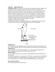
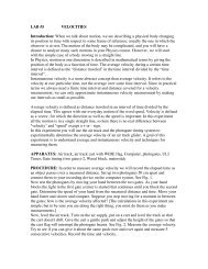
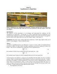
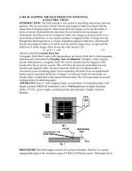
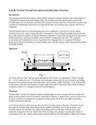
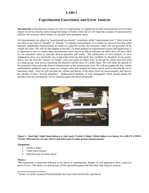
LAB# 2Experimental Uncertainty and Error AnalysisIntroduction: In the physical sciences as well as in engineering, we depend on accurate measurements of real-worldobjects to test our theories and to design the things we build. In this lab we will study the accuracy of measurementsand how this accuracy affects things we calculate from measured values.All measurements are subject to "experimental uncertainty", sometimes called "experimental error". These terms donot refer to any kind of "mistake" or “blunder” 1 in making measurements. It is simply an observed fact that whenrepeated, independent measurements are made on a physical system, the measured values will not generally all beexactly the same. (We will see this happen in this lab.) To make progress in experimental science and engineering, itis important to strive to reduce these measurement errors, and to be able to calculate the effect they will have whenwe use measured values to calculate desired quantities and results. The mathematics of error analysis, or errorpropagation, gives us a systematic way to determine from our data itself, how confident we should be of our results;that is, how far from the "correct" or "actual" value our results are likely to be. In this lab the whole class will workas a large group, each person measuring the diameter and the mass of a metal object. We will study the spreads ofthe measured values and relate them to characteristics of the measurement tools. We will see graphically how certainmathematical quantities such as mean (or average) value and standard deviation can be used to describe the set ofmeasured values. Next we will calculate the volume and density of the object from our measurements, and observethe spreads of these "derived quantities". Mathematical formulae of error propagation which should predict thespreads in the derived quantity, will be checked against the observed spreads.Figure 1. Steel ball, triple beam balance, a ruler and a Vernier Caliper. Metal calipers are sharp. Use with CUATION.Vernier Micrometers are also shown and often used to make precise measurements.Equipment:1. Vernier Caliper.2. Triple-beam balance.3. Steel ball (one for entire class).Theory:This experiment is somewhat different as the theory is mathematical, though we will approach it from a physicalpoint of view. The theory we shall discuss will be spread throughout the Procedure and Analysis sections.1In fact, we tacitly assume all human blunder has been removed from the experiment.

(Hint: Fill in the open circles in front of the procedure steps to help you perform the experiment)Procedure:In this part of this lab we will study the measurement process itself. That is, the fact that each and everymeasurement ever made has some uncertainty. There is no such thing as a “Perfect Measurement”. You can seeone aspect of this inability to make a perfect measurement quite easily. What if a measurement comes out betweenthe finest markings on your measurement scale? What value would you assign to this measurement? There is noway to be certain of this value. Each member of the entire class will measure the diameter and the mass of a singlesteel ball. This procedure is supposed to simulate the situation of one person making a number of independentmeasurements of the ball. Follow your TA's instructions on how to use the Vernier caliper 2 and the triple-beambalance to measure the ball. It is important that each person measure the ball independently; don't influence eachother's measurements by discussing technique or comparing values. No one will keep track of who got what values.Your grade will not depend on "your" measured values at all. Make your measurement by yourself and report itquietly to your TA, who will collect all the data on the chalkboard. Finally, each of you should collect the wholeclass' measurements of the diameter and the mass of the ball into your own data table like the one shown below. Becertain to measure the diameter and mass to the maximum accuracy available on your apparatus.In short:o Measure the diameter of the steel ball using the Vernier calipers (see Appendex A).o Measure the mass of the steel ball using the triple-beam balance.o Fill in the table below using the measurements of the entire class.Trial Diameter (cm) Mass (g) Volume(cm 3 ) Density(g/cm 3 )MeanStd.DeviationAnalysis:Calculate the mean (average) and the standard deviation for the diameter and the mass measurements. The formulaefor mean and standard deviation are given in the Appendix of the lab manual, and in the Handbook of Chemistry andPhysics or similar references. Some calculators have these functions built-in; you can also use the spreadsheet2You may also wish to consult http://members.shaw.ca/ron.blond/Vern.APPLET/index.html, which has a very niceapplet on how to read Vernier Calipers.

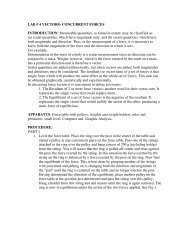
program, Excel or the Graphical Analysis program, to calculate these. Enter the mean and standard deviation into the tablein the indicated cells. Typically one takes an average value to be their best measurement and the standard deviationto be a measure of the spread in their measurements.Make a frequency distribution, or also called a histogram, for the diameter measurements. What we are trying to dohere is determine how often given measurements of the diameter occurred. That is, are all the measurements aboutthe same, are they all “bunched-up” about one value? Or, are they greatly spread out over a wide range of values.Perhaps most are very close in value with one or two values being very different from the rest (we call theseoutliers). There are many possibilities, but a histogram will give us a visual picture as to how precise our bestmeasurement is (Precision refers to how closely individual measurements agree with each other, accuracy refers tohow closely a measured value agrees with the correct value).Typically one would use some computer application to make a histogram. You could use Microsoft Excel, or theGraphical Analysis package on your lab computer. You should be aware that if you decide to make a histogram byhand the choice of bin size and number of bins is a tricky statistic question. You may wish to consulthttp://davidmlane.com/hyperstat/A28364.html for more information. An example histogram is shown below. Itrepresents the number of times a given measurement fell into a certain range or “bin” (the fraction of thatmeasurement to the total number of measurements). Note Well: The ranges or bins touch, but do not overlap.Questions:Figure 2: Example Histogram showing frequency of diametermeasurements1. According to statistical theory, if the errors in the measured values are small and truly random, then 68% ofthe values should lie within plus or minus one standard deviation from the mean value. Does your class'data approximately satisfy this rule? If not, study the histogram and try to state a reason why yourdata might not satisfy this rule.2. Let us try to understand the meaning of the standard deviation in terms of the measurement process itself.How precise would you expect the length measurements to be? What about the mass measurements?Consider the following:a. What is the smallest division you can read on the Vernier scale of the calipers?b. How much must you move the smallest sliding weight on the triple-beam balance to noticeablychange the balance condition?

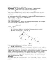
c. Compare the standard deviations of the measured data sets with the expected precisionsfrom the preceding question. Are they similar? (They should be.) If not, study the histogramand try to see why your class' data may not be behaving as it should.From the preceding exercises we should hopefully learn that: Repeated, independent measurements of a quantitywill vary about the average measured value. The majority of measurements lie within one standard deviation of themean. Thus we can be reasonably confident that if we had measured the quantity only once, that value would differfrom the mean of many repeated measurements by at most a standard deviation or so. The standard deviation foundon repeated measurements will be similar to the precision of the measuring equipment (at best). Thus if we knowonly one measured value and something about the equipment, we can have an idea of the likely difference betweenour measured value and the mean of a large number of repeated measurements. One or two measured values whichlie far from the mean ("outliers") can strongly influence the calculated standard deviation. There are many reasonswhy outliers can occur. Occasionally they may represent "mistakes" in the measurement procedure, rather thanchance fluctuations, but one must be very careful not to assume this. There are statistical tests which we will notdiscuss, that can show whether it is mathematically reasonable to discard such outliers. In some cases outliers shownew and interesting phenomena and scientist mine data looking for such occurrences.Uncertainty in Derived Quantities; Error Propagation:Typically the value of the physical parameter of interest is not obtainable from one measurement. In nearly all casesone must combine a number of measurements to arrive at the final desired result. What we are interested in studyingin this part of our experiment is how experimental uncertainties in our measured values propagate through ourcalculations and affect the certainty of our final result. Not taking this propagation of error volumes into accountcorrectly can have disastrous results (see the figure below of the train accident). We will study this effect byanalyzing how the uncertainty in our measured values of diameter and mass effect calculations of the balls volumeand density. Along the way we will learn some rules for error propagation.oCalculate the volume of the ball from each diameter measurement using the formula, and enter the values inyour table.34 ⎛ d ⎞V = π ⎜ ⎟ ,3 ⎝ 2 ⎠(1)ooCalculate the mean and standard deviation of the volume data set and enter them into your table.Calculate the density of the ball from each volume value and mass measurement using the formula and enter thevalues into your table.mρ = ,V(2)oCalculate the mean and standard deviation of the density data set and also enter them into your table.Questions:Let us try to understand the scatter in the calculated volume values, which arises from the scatter in the diametermeasurements. What we mean is that the uncertainty, or error, in the measurements of the diameter leads touncertainty in the calculated volume values. We now investigate how one can deduce the uncertainty in thecalculated volume value based on the uncertainty in the diameter value. Obviously one would not calculate thevolume 20 different times using the 20 different values of the diameter. That would be a waist of time (however, weperform this exercise here to convince ourselves that the methods we are about to present truly work – and tounderstand how). What we want are the rules for propagating the uncertainty in the “best measurement” of the

diameter to a “best calculated” value of the volume. The mathematical rules for propagating errors can be derivedusing calculus. We will simply present the results here.CABCCAXBA/B(3)CnAIn Equation (3) we use the symbol σ C for the uncertainty in the value of C. Notice how the errors do not just add.The squares of the uncertainties are squared, than added, than the square root is taken. This is called “added inquadrature” and this rule for propagating uncertainties is a result of statistics and probability.As you can see the error propagation formulae often involve "relative uncertainties". That is, the uncertainty(standard deviation) divided by the mean value. (This could also be multiplied by 100 to get the "percentuncertainty".) Relative uncertainty gives a measure of the magnitude of the uncertainty, taking into account themagnitude of the average measurement. Consider: Your uncertainty could be 1 mile, but if we are talking about themeasurement of the distance from here to the moon that would be quite small.Calculate the mean and standard deviation for the volume data set (the volumes calculated from your individualdiameter measurements and equation above). Now use the error propagation rules above and calculate a best valueand uncertainty for the volume of the ball using the mean and standard deviation of the ball. How well do theaverage of the volume data set and the best value, calculated using propagation of error, compare? How well do thestandard deviation of the volume data set and the uncertainty using propagation of error compare?At this point you may be thinking that this is all very nice, but has no usefulness in the “real world”. Nothing can befurther from the truth. Say, for example, you were hired by Bill Gates to fill his swimming pool with Champagne.(Or by your uncle to fill a foundation form with cement.) You measure the length, width and depth of the pool andmultiply them together to get the volume, but how far off might the calculated volume be? If it is too small, youwon't order enough Champagne, Bill's guests will be disappointed, and you'll get fired. If it is too big you'll wastehis money ordering too much, Bill will find out, and you'll get fired. But if you have an idea of the uncertainty of thelength, width and depth measurements, and you know the error propagation formulae, you can predict theuncertainty in the volume, order just enough to be confident the pool will be filled, and save your job. In the case ofcement there is the added complication that cement is ordered by weight, so you would need to calculate the weightrequired and its associated uncertainty. But the method and the consequences (for your job) would the same.Worse yet, if you were the engineer whose job it was to design a rail system and you didn’t take uncertaintiesproperly into account, look what could happen.

From this section we have hopefully learned that in order to get the best estimate of a derived quantity, such asdensity, one can take multiple independent measurements of the input quantities (i.e. mass, diameter), and thancalculate the derived quantity using the various combinations of the input quantities. The mean of the derivedquantity would then represent our best estimate, while the standard deviation would represent the uncertainty in ourderived quantity. Hopefully though, while we see this is a useful exercise to build understanding and intuition, itwould be a terrible practice. We should instead make a best measurement of our input quantities, using the smallestdivision on our measuring apparatus as a measure of our uncertainty 3 . Then using our best measurements of ourinput parameters calculate a best estimate of our derived quantity. The uncertainty in our derived quantity can beobtained using our rules for error propagation.Final Note:In the above discussions, we have tacitly assumed that a large number of independent measurements will clusteraround the "true value" of the quantity being measured. We have used the spread of values as an indication of howfar from the "true value" our measurements are likely to be. This is reasonably true in many cases. The scatter iscalled indeterminate (or random) uncertainty. Often, however, there is some bias in the measurement tools orprocedure which causes all the measured values to tend to be too low or too high. For example, the calipers might bemade of some kind of plastic that shrinks as it ages. Or the triple-beam balance may not be properly zeroed. Thenthe large number of independent measurements will not cluster around the "true value" of the quantity beingmeasured. This is called systematic (or determinate) "error". It is also very important (and troublesome!) inexperimental science, but we do not study it here. Systematic errors can only be estimated by detailed study of theparticular measurement tools and method being used.3Typically, we use “± ½ the smallest division” of our measuring apparatus as the uncertainty in our measurement.

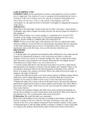
Appendex AHow to use the vernier caliper:If you are unfamiliar with the use of the vernier caliper, the lab instructor will explain itfor you using a demonstration model. A diagram is presented below.There are two scales on the vernier caliper instrument, the top two scales use inches, andthe bottom two scales use millimeters. Let’s see how we read a measurement of length of 14.65.Note: The scale that runs from 0 to 130 (your caliper might run to 120), we are going tocall this scale the top scale. Each of those divisions is 1 mm. Note the smaller scale right below,the one that starts with 0 and ends with 0, with 0.05 mm written beside it, each division on thisscale is 0.05mm.Line up the first 0 on the smaller scale with the number above it on the larger scale. This0 falls between 14 and 15 mm on the larger scale. That means that the jaws are open between 14and 15 mm. This gives us the whole mm part of the measurement. Now look on the smallerscale, and see where the line, or tick mark, of the smaller scale, lines up best with a line on theupper scale. The line between 6 and 7 lines up very well with line for 40 on the upper scale, thisis .65mm, the fractional part of the measurement.To get the final answer, we add the two numbers, 14 and .65, for 14.65mm. Note thatsince the fractional scale is divided up in 0.05mm steps, the last digit in our measurements willbe a 0 or 5.The calipers need some practice, so give yourself the time you need, and ask your TA forhelp if it is not clear.