Homework 2 Solution (pdf)

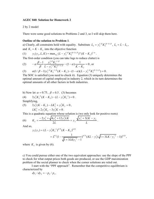
AGEC 840. Solution for Homework 22 by 2 modelThere were some good solutions to Problems 2 and 3, so I will skip them here.Outline of the solution to Problem 1.1/ β ( β −1)/ βa) Clearly, all constraints hold with equality. Substitute L2= y2K2, L1 = L − L2,and K = K − into the objective function1K 21/ β ( β −1) / β α1−α(1) y ( y , L,K)= max ( L − y K ) ( K − K .21 2K 2 22)The first-order condition (you can take logs to reduce clutter) is1/ β −1/ββ − 1 y K21(2) − α2 − (1 − α)= 0, or1/ β ( β −1) / ββ L − y KK − K221/ β −1/β1/ β ( β −1) / β(3) α(1/β − 1) y2 K2( K − K2) − (1 − α)(L − y2K2) = 0 .The SOC is satisfied (you need to check it). Equation (3) uniquely determines theoptimal amount of capital employed in industry 2, which in its turn determines theoptimal amounts of all other factors in both industries.2b) Now let α = 0. 75, β = 0. 5 . (3) becomes(4)2 −22 −13y2 K2( K − K2) − ( L − y2K2) = 0 .Simplifying,(5)22 23y2 ( K − K2) − LK2+ y2K2= 0 ,2 22LK2+ 2y2K2− 3y2K = 0 .This is a quadratic equation whose solution is (we only look for positive roots)(6)24 22− 2 y2+ 4 y2+ 12 y2LK y2+ 3LK− y2K2= = y2.2LLAnd so,2 −10.750.25y 1( y 2) = ( L − y2 K2) ( K − K2)0.5 10.752−20.25= L ( 1 −) ( KL − y22( 1 + 3LK/ y2− 1)) ,−1 + 3LKy2− 1where K 2is given by (6).c) You could pursue either one of the two equivalent approaches: use the slope of the PPFto check for what output prices both goods are produced, or use the GDP maximizationproblem of the social planner to check when the corner solutions are ruled out.I start with the “PPF approach”. Remember that the competitive equilibrium ischaracterized bydy / dy = − p p ,1 2 2/1

i.e., the economy produces outputs where the PPF is tangent to the price line (the“economy’s budget constraint”). And so, both goods will be produced as long as− dy2( y1= f1(L,K)) / dy1> p1/ p2and− dy1( y2= f2(L,K)) / dy2> p2/ p1.Differentiating (1) yieldsdy / dy 1/ β ( β −1) / β α −11−α1/ β −1( β −1) / β1 2= α(L − y2 K2) ( K − K2) (1/ β ) y2K2,where we used the FOC to eliminate dy1/ dK2= 0 (the envelope theorem). Using theFOC for the PPF, (2) or (3), we have1/ β ( β −1) / β1/ β −1/β( L − y2 K2) = ( α /(1 − α))((1− β ) / β ) y2K2( K − K2).Substitute this into dy / dy 1 2to get− dy / dy α K − K2 1−αy2(1−β) / β1 2= () ( )1/ β −1/ββ ( α /(1 − α))((1− β ) / β ) y2K2( K − K2) K2α 11−αy2( α −1) / β y2(1−β) / β= () ( ) ( )β ( α /(1 − α))((1− β ) / β ) K2K2α 11−αy2( α −β) / β= () ( )β ( α /(1 − α))((1− β ) / β ) K2α (1 − α)β 1−αL2α −β= ( ) ( ) ,β α(1− β ) K21/ β2/ K2( y2/ K2)y ( 2= f2L,K)where L = is used (from the constraint that the output of good 2 is y2).Evaluating at , L2= L, K2= K yieldsα (1 − α)β 1−αL α −βp2− dy1 ( y2= f2(L,K))/ dy2= ( ) ( ) >β α(1− β ) K p1For concreteness, suppose that α > β . Then we obtain1/( β −α)L ⎛ p1 ⎞ α (1 − α)β 1−α1/( β −α) ⎛ p> ⎜⎟ ( ( ) ) =K ⎝ p2 ⎠ β α(1− β )⎜⎝ p1−αα β β 1−βwhere H ≡ ( ) ( ) .α 1−β 1−αThe upper bound is found similarly (check this).⎞⎟⎠1/( β −α)1 1/( α −β)H2β,1 − βAlternatively, to answer this question you could set up the GDP maximizationproblem:GDP( p = y subject to1,p2, L.,K ) maxL 1,K1,L2, K 2 , y,yp2 1y1+ p22α 1−αβ 1−βy1≤ L1K1, y2 ≤ L2K2, L + L 2≤ Ly1≥ 0,y2≥ 0, L1≥ 0, L2≥ 0, K1≥ 0, K2≥1, K + K 2≤ K01,and determine conditions under which a corner solution is optimal. First, write down theoptimality conditions assuming that it is optimal to produce both goods, and then usethem to determine conditions under which they are satisfied for positive outputs (i.e., it is

Now solve (FE) to determine the optimal outputs (if both goods are produced)⎛ a1La2L⎞⎛y1⎞ ⎛ L ⎞⎜ ⎟⎜⎟ = ⎜ ⎟⎝a1Ka2K⎠⎝y2⎠ ⎝ K ⎠Inverting the technology matrix yields−1⎛ y1 ⎞ ⎛ a1La2L⎞ ⎛ L ⎞ 1 ⎛ a2L− a2L⎞⎛L ⎞⎜⎟ =⎜⎟ ⎜ ⎟ =⎜⎟⎜⎟⎝ y2⎠ ⎝a1Ka2K⎠ ⎝ K ⎠ a1La2K− a1Ka2L⎝−a1Ka1L⎠⎝K ⎠1 ⎛a2LL− a2LK⎞=⎜⎟ .a1La2K− a1Ka2L⎝ a1LK − a1KL ⎠As before, for concreteness, suppose that α > β , then a1 La2K− a1Ka2L> 0 by (7). Andso, y > 0 and y > 01 2, if and only if⎧a2LL− a2LK> 0 a2LL a1L⎨, or < < .⎩a1LK− a1KL > 0 a2KK a1KSubstitute (8) to get(9)⎛ p⎜⎝ p⎞⎟⎠1/( β −α)⎛ p ( < ) ,p f ( L / K,1)21( 1f1 L,Kwhere y = ) and y ( 2= f2L,K). In Problem 4, you are asked to show that theright-hand side of the last inequality decreases with L / K . Note that the Cobb-Douglastechnologies satisfy the assumptions (1) – (3) in Problem 4. Therefore, it is more likelythat the economy will specialize in the labor-intensive good (good 1) when thelabor/capital ratio of factor endowments is high (labor-abundant country), andconversely. Note that the same logic applies in the case of factor-intensity reversalswhen the ratio of factor endowments falls in between the “cones of diversification”.

Problem 4. Creative assignment for extra-credit:Suppose that in a 2 by 2 economy the endowment of labor increases. Can you show thatas the PPF expands it will stretch towards the labor-intensive good as illustrated in Figure1.10 on page 21 in Feenstra? Try to show this without relying on specific functionalforms but just employing the three assumptions imposed on the production technology:(1) higher inputs lead to higher outputs, (2) balanced inputs lead, on average, to higheroutputs, and (3) constant returns to scale.Proof: There are two steps. First, we use the assumption that industry 1 is laborintensiveto see what it tells us about the production functions. Second, we use thatinformation to compare the percentage changes in the maximal outputs of each good theeconomy can produce for given changes in the factor endowments.Step 1. Note that the optimal factor requirements satisfy (see the definition of the unitcost function) the following optimality condition:wrf1L( a1L, a1K) f2L( a2L,a2K)= =, orf ( a , a ) f ( a , a )1K1L1K2K2L2Kff1L1K( a( a1L1L/ a/ a1K1K,1),1)f2L( a2L/ a2K,1)= .f ( a / a ,1)2K2L2KBy assumption, a1L ( w,r)/ a1K( w,r)> a2L(w,r)/ a2K( w,r)for all factor prices. Then, byconcavity and homogeneity of the production functions, it follows thatff1L1K( a( a1L1L/ a/ a1K1K,1),1)f2L( a2L/ a2K,1) f2L( a1L/ a1K,1)= >, orf ( a / a ,1) f ( a / a ,1)2K2L2K2K1L1Kf1L ( x,1)f2L( x,1)> ∀x .f ( x,1)f ( x,1)1K2KStep 2. The endpoints of the PPF are y ( 1= f1 L,K)and y ( 2= f2L,K). The PPFstretches towards good 1 as the labor endowment increases when d ( y1 / y2) / dL > 0 .d1 dy1dy2y1 / y2) / dL = ( y2− y ) >2( y ) dL dL(120 , or1y1dy1dL1 dy2> .y dL2To show the last inequality, rewrite it asf1L ( L,K)f2L( L,K)> , orf ( L,K)f ( L,K)12

f1Lf1L( L,K)L( L,K)L + f ( L,K)K1K>f2Lf2L( L,K)L, or( L,K)L + f ( L,K)K2Kf2 K( L,K)K f1K( L,K)K1 + > 1 +, orf ( L,K)L f ( L,K)L2L1Lf1L ( L,K)f2L( L,K)> , orf ( L,K)f ( L,K)1K2Kf1L ( L / K,1)f2L( L / K,1)> ,f ( L / K,1)f ( L / K,1)1K2Kwhich holds by Step 1 for anyL / K . And so, we showed that d y / y ) / dL 0 . ■(1 2>