
You also want an ePaper? Increase the reach of your titles
YUMPU automatically turns print PDFs into web optimized ePapers that Google loves.
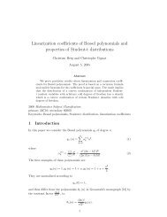
<strong>Barrier</strong> <strong>Options</strong> <strong>and</strong> <strong>Lumpy</strong> <strong>Dividends</strong><br />
Johannes Vitalis Siven ∗<br />
Michael Suchanecki †<br />
Rolf Poulsen ‡<br />
February 24, 2009<br />
Abstract<br />
We study the pricing of barrier options on stocks with lumpy dividends. By ex-<br />
tending the European option methodology presented in Haug, Haug & Lewis (2003),<br />
we show that in the Black-Scholes model with a single dividend payment, barrier<br />
option prices can be expressed in terms of well-behaved one-dimensional integrals<br />
that can be evaluated very rapidly. With multiple dividend payments, the price<br />
integrals are more involved, but we show that for the down-<strong>and</strong>-out call option a<br />
simple approximation method gives accurate results.<br />
Keywords: <strong>Barrier</strong> options, lumpy dividends, numerical integration, finite dif-<br />
ference method, down-<strong>and</strong>-out call.<br />
1 Introduction<br />
Dividend payments impact stock price dynamics <strong>and</strong> consequently the pricing of<br />
equity derivatives. The common solution of approximating lumpy dividends with a<br />
∗ Saxo Bank, Philip Heymans Allé 15, DK-2900 Hellerup, Denmark. E-mail: jvs@saxobank.com<br />
† HSBC Trinkaus & Burkhardt, Königsallee 21/23, D-40212 Düsseldorf, Germany. E-mail:<br />
michael.suchanecki@hsbctrinkaus.de<br />
‡ Department of Mathematical Sciences, University of Copenhagen, Universitetsparken 5, DK-2100<br />
Copenhagen, Denmark. E-mail: rolf@math.ku.dk<br />
1
continuous dividend yield works reasonably well for stock indices, 1 but the discrete-<br />
ness of dividends cannot be ignored for derivatives written on individual stocks.<br />
This issue becomes even more acute for barrier options than for plain-vanilla Euro-<br />
pean options, essentially because dividend payments affect not only the stock price<br />
distribution at expiry, but also the probability of barrier crossings.<br />
The literature contains a number of suggestions for how to adjust derivative<br />
prices for discrete dividends in the underlying stock, see for instance Beneder &<br />
Vorst (2001), Bos, Gairat & Shepeleva (2003), Chriss (1997) <strong>and</strong> Frishling (2002).<br />
However, as discussed extensively in Haug et al. (2003), there are various prob-<br />
lems with all of these approaches, ranging from ill-defined stock prices to poor<br />
performance of approximations in particular situations. Haug et al. (2003) resolve<br />
these issues by proposing a rigorous, yet natural, method for pricing European-type<br />
derivatives in the case of a single dividend — we describe the approach in Section<br />
2.<br />
In Section 3, we extend the methodology to barrier options. The key observation<br />
is that while barrier options are path-dependent, they are only weakly so — given<br />
that a barrier option has not yet been knocked out, the price is a function only of<br />
time <strong>and</strong> the current stock price. We show that in the Black-Scholes model with<br />
a single dividend payment, the barrier option price is a one-dimensional integral of<br />
Black-Scholes-type functions against a log-normal density which is straightforward<br />
to evaluate numerically.<br />
The case of a single dividend is the most relevant by far since dividends are<br />
usually paid yearly <strong>and</strong> most derivatives — especially exotic ones — have much<br />
shorter life-spans than that. For a point in case, so-called Turbo warrants typically<br />
expire within one year. These contracts are popular in many countries because they<br />
enable retail investors to acquire the payoff profile of a barrier option. 2<br />
Section 4 demonstrates that the proposed numerical integration method is signif-<br />
icantly faster than a general purpose attack on the problem — solving the pricing<br />
PDE with the Crank-Nicolson finite difference scheme. In Section 5, we look at<br />
1 It is important to account for the seasonality in dividend payments. To quote a practitioner who<br />
shall remain nameless: “In other words - don’t try using constant div-yield BS, even on indices”.<br />
2 Turbo warrants usually come in two forms — the long version is a regular down-<strong>and</strong>-out call (barrier<br />
lower than or equal to the strike) <strong>and</strong> the short version is a regular up-<strong>and</strong>-out put (barrier higher than<br />
or equal to the strike) — see Mahayni & Suchanecki (2006), Engelmann, Fengler, Nalholm & Schwendner<br />
(2007), Wilkens & Stoimenov (2007) <strong>and</strong> Wong & Chan (2008).<br />
2
multiple dividends <strong>and</strong> show that an approximation approach similar to the one<br />
considered for plain-vanilla options in Haug et al. (2003) is feasible for the down-<br />
<strong>and</strong>-out call option.<br />
2 European options for single dividends<br />
This section reviews the approach from Haug et al. (2003) for pricing European-style<br />
contracts written on a stock that pays a single dividend.<br />
Fix a time interval [0,T] <strong>and</strong> consider the stock price for a company that pays<br />
the dividend d at a deterministic time τ ∈ (0,T) <strong>and</strong> that the size of the dividend<br />
is anticipated in the market prior to τ (“Fτ−-measurable” if you like). A simple<br />
arbitrage argument shows that the stock price will decrease by d at the same instant<br />
as the dividend is paid. Let r ≥ 0 denote the interest rate <strong>and</strong> let (St) t∈[0,T] model<br />
the price of the stock under the risk-neutral measure:<br />
dSt = rStdt + σStdWt, when 0 ≤ t < τ or τ < t ≤ T,<br />
Sτ = Sτ− − d, otherwise,<br />
where (Wt) t∈[0,T] is a st<strong>and</strong>ard Brownian motion. Companies usually declare a<br />
dividend size D in advance, but for the model to be well defined one has to be<br />
careful <strong>and</strong> not assume that the actual dividend d is deterministic — if the stock<br />
price happens to be less than that constant at time τ−, the company is unable to pay<br />
the declared dividend — we must have that 0 ≤ d ≤ Sτ−. This technicality, which<br />
is ignored for instance by Frishling (2002) <strong>and</strong> Bos et al. (2003), can be resolved by<br />
assuming that d = d(Sτ−) is a deterministic function of the stock price the instant<br />
prior to the dividend payment. Haug et al. (2003) consider d(s) = min{s,D} (“the<br />
liquidator”) <strong>and</strong> d(s) = D1 {s>D} (“the survivor”) for a given deterministic D ≥ 0.<br />
Another natural choice would be d(s) = αs for some constant α with 0 < α < 1 —<br />
a proportional dividend.<br />
Let C(t,s) = e −r(T −t) E[(ST − K) + |St = s] denote the price at time t of a Euro-<br />
pean call option with strike K <strong>and</strong> expiry T, given that St = s. At time τ, the one<br />
<strong>and</strong> only dividend has been paid, hence the stock price follows a geometric Brownian<br />
motion on [τ,T] — the price C(τ,s) is thus the usual Black-Scholes price. Now, to<br />
compute the price of the contract at time 0, simply condition on the information<br />
3<br />
(1)
available at time τ:<br />
e −rT E[(ST − K) + ] = e −rτ E[e −r(T −τ) E[(ST − K) + |Sτ]]<br />
= e −rτ E[C(τ,Sτ)]<br />
= e −rτ E[C(τ,Sτ− − d(Sτ−))]. (2)<br />
The last expectation is a one-dimensional integral of the function s ↦→ C(τ,s−d(s))<br />
multiplied by a log-normal density <strong>and</strong> can easily be evaluated numerically.<br />
The method is valid not only for the plain-vanilla European call option, but<br />
generally for contracts with payoff f(ST) at time T, provided that the function<br />
s ↦→ E[f(ST)|Sτ = s] is available in closed form, or at least is easy to compute.<br />
Moreover, it is valid for more general models than the geometric Brownian motion.<br />
As long as the density of the stock price at the instant prior to the dividend payment<br />
is available, then the expectation (2) can be computed by numerical integration.<br />
3 <strong>Barrier</strong> options for single dividends<br />
We now extend the approach described in the previous section to treat barrier<br />
options in the case of a single discrete dividend. For concreteness, we specialize in<br />
a down-<strong>and</strong>-out call option, but it is easy to see that similar calculations work for<br />
other contracts, in particular for the other single barrier options.<br />
We compute the price at time 0 of a down-<strong>and</strong>-out call option with expiry T,<br />
strike price K, barrier L, with 0 ≤ L ≤ K, written on the dividend-paying stock.<br />
This contract is a contingent claim with time-T payoff<br />
(ST − K) + 1 {min0≤t≤T St>L}. (3)<br />
At time τ, the one <strong>and</strong> only dividend has been paid, hence the stock price follows<br />
a geometric Brownian motion on [τ,T]. From Björk (2004, Proposition 18.17), we<br />
have that the price of the contract at time τ is P(τ,Sτ), where<br />
P(τ,s) :=<br />
�<br />
C(τ,s) −<br />
� L<br />
s<br />
� p<br />
C<br />
�<br />
τ, L2<br />
s<br />
��<br />
1 {s>L}, (4)<br />
with p := 2r<br />
σ 2 − 1. As in the previous section, C(τ,s) denotes the usual no-dividend<br />
Black-Scholes price at time τ of a European call option with strike K <strong>and</strong> expiry T.<br />
The key observation that enables us to compute the price at time 0 of the claim<br />
(3) is that at time τ, given that the barrier has not yet been crossed, the value of<br />
4
the option is precisely P(τ,Sτ) = P(τ,Sτ− − d(Sτ−)). Consequently, at time 0 we<br />
can view the barrier option we are trying to price as a contingent claim with expiry<br />
τ <strong>and</strong> payoff<br />
P (τ,Sτ− − d(Sτ−))1 {min0≤t≤τ− St>L}.<br />
But this is just a down-<strong>and</strong>-out option with an unusual payoff written on a geometric<br />
Brownian motion — the stock price follows a geometric Brownian motion on [0,τ).<br />
It follows from Björk (2004, Theorem 18.8) that the price at time 0 of the claim is<br />
P(0,S0) := e −rτ<br />
� � �p � ��<br />
L L2 I(S0) − I 1 {S0>L}, (5)<br />
where<br />
⎡<br />
⎢<br />
I(s) := E ⎣P<br />
g(s) := s − d(s).<br />
� � “<br />
τ,g se<br />
r− σ2<br />
2<br />
S0<br />
” ��<br />
τ+σWτ<br />
1 (<br />
g<br />
S0<br />
se<br />
„<br />
r− σ2<br />
2<br />
« !<br />
τ+σWτ<br />
>L<br />
)<br />
⎤<br />
⎥<br />
⎦ , (6)<br />
Consider the dividend policy of “the liquidator”, i.e. d(s) = min{s,D} for some<br />
deterministic D ≥ 0. The expectation (6) becomes<br />
I(s) =<br />
c(s) :=<br />
� ∞<br />
c(s)<br />
P<br />
log � L+D<br />
s<br />
�<br />
τ,g<br />
� �<br />
−<br />
σ √ τ<br />
� “<br />
se<br />
r− σ2<br />
2<br />
r − σ2<br />
2<br />
”<br />
τ+σ √ τy<br />
�<br />
τ<br />
,<br />
��<br />
N ′ (y)dy,<br />
where N ′ (·) denotes the density of the st<strong>and</strong>ard normal distribution. The two inte-<br />
grals in (5) have to be computed numerically, but this is easily done: the integr<strong>and</strong>s<br />
are smooth <strong>and</strong> decay extremely fast as y → ∞ due to the factor N ′ (y). Greeks<br />
can be computed by evaluating the same kind of integrals.<br />
4 Numerical experiments<br />
In this section, we perform numerical experiments with the proposed numerical inte-<br />
gration method for pricing a down-<strong>and</strong>-out call option. The method is benchmarked<br />
against a general purpose approach to the problem — solving the pricing PDE with<br />
a finite difference scheme. The computations are done using the software R on an<br />
ordinary work station <strong>and</strong>, unless stated explicitly, all experiments are conducted<br />
using the parameters in Table 1.<br />
5
Quantity Symbol Value<br />
call strike K 100<br />
knock-out barrier L 95<br />
initial spot S0 K<br />
barrier option expiry T 0.2<br />
dividend date τ T/2<br />
interest rate r 0.05<br />
stock volatility σ 0.1<br />
Table 1: Parameters in the numerical experiments.<br />
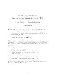
Consider the price at time 0 of the down-<strong>and</strong>-out call option when the underlying<br />
stock pays a dividend d = min{Sτ−,D} at time τ, where D ≥ 0 <strong>and</strong> 0 < τ < T.<br />
Figure 1 shows the price as a function of D <strong>and</strong> τ. The dividend makes barrier<br />
crossings more likely since the contract is down-<strong>and</strong>-out <strong>and</strong> makes the option more<br />
out-of-the-money. So, the price is a decreasing function of D for each fixed τ. For<br />
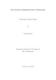
D = 0, we obtain the usual no-dividend Black-Scholes price of 2.2981. Figure 2<br />
shows the price as a function of τ for D = 2,5 <strong>and</strong> 8. We see that the timing of the<br />
dividend is more important for large dividends <strong>and</strong> that the contract is cheaper the<br />
earlier the dividend is paid.<br />
4.1 Comparison with the Crank-Nicolson scheme<br />
Since the underlying has geometric Brownian motion dynamics everywhere except<br />
when the dividend is paid, the price at time t of the contract is given by P(t,St),<br />
where P(t,s) solves<br />
∂P<br />
∂t<br />
1<br />
+<br />
2 σ2s 2∂2P + rs∂P − rP = 0<br />
∂s2 ∂s<br />
for t ∈ [0,T], t �= τ, <strong>and</strong> s > L. The boundary <strong>and</strong> terminal conditions are given by<br />
P(t,L) = 0, for t ∈ [0,T],<br />
P(T,s) = max{s − K,0}, for s > L,<br />
<strong>and</strong> the behavior at the dividend payment date τ is given by the following jump<br />
condition:<br />
P(τ−,s) = P(τ,s − d(s)).<br />
6<br />
(7)
price<br />
2.5<br />
2<br />
1.5<br />
1<br />
0.5<br />
0<br />
0.2<br />
0.15<br />
0.1<br />
0.05<br />
τ<br />
0<br />
10<br />
Figure 1: Price at time 0 of the down-<strong>and</strong>-out call option as a function of the dividend<br />
size D <strong>and</strong> payment time τ.<br />
This PDE can be solved numerically with finite difference schemes — the domain<br />
[0,T] × [L, ∞) is truncated for some large s-value <strong>and</strong> discretized using some fi-<br />
nite step sizes ∆t <strong>and</strong> ∆s, <strong>and</strong> the partial derivatives are approximated by finite<br />
differences. The Crank-Nicolson scheme is (at least locally) second-order accurate<br />
in both time <strong>and</strong> space <strong>and</strong> is frequently chosen in the finance literature <strong>and</strong> in<br />
practice. We refrain from describing it here <strong>and</strong> instead refer to Wilmott (2006)<br />
for a nice explanation of the method. He also discusses various implementational<br />
issues, including the need for interpolation when the dividend size is not an inte-<br />
ger multiple of ∆s. However, we note that there are potential pitfalls — Duffy<br />
(2004) discusses problems with the Crank-Nicolson scheme in situations with irreg-<br />
ular boundary conditions — it is therefore important to investigate the convergence<br />
in our particular setting.<br />
We choose the asset step proportional to the time step, ∆s = c∆t. Using the<br />
analysis from Østerby (2008, Chapter 10) we find that the value c = 12.5 is optimal<br />
for computational efficiency — this choice gives errors of approximately the same<br />
size in the asset dimension <strong>and</strong> in the time dimension.<br />
Table 2 reports the error for the prices computed with the Crank-Nicolson scheme<br />
relative to the exact price computed by numerical evaluation of (5). We note that the<br />
table confirms the second-order accuracy of the PDE solution method — doubling<br />
7<br />
8<br />
6<br />
D<br />
4<br />
2<br />
0
price<br />
1.4<br />
1.2<br />
1<br />
0.8<br />
0.6<br />
0.4<br />
0.2<br />
0<br />
0 0.02 0.04 0.06 0.08 0.1<br />
τ<br />
0.12 0.14 0.16 0.18 0.2<br />
Figure 2: Price at time 0 of the down-<strong>and</strong>-out call option as a function of the payment<br />
time τ for D = 2 (solid), D = 5 (dotted) <strong>and</strong> D = 8 (dashed).<br />
the number of asset <strong>and</strong> time steps reduces the error roughly by a factor of four. It<br />
also doubles the number <strong>and</strong> the size of the systems of linear equations that must<br />
be solved <strong>and</strong> hence quadruples computation time. 3 Evaluating (5) takes only 0.02<br />
seconds, so it is clear that the numerical integration method is significantly faster<br />
than the Crank-Nicolson scheme.<br />
5 Approximation for several dividends<br />
In this section, we discuss an approximation approach for pricing the down-<strong>and</strong>-<br />
out call option in the case of multiple dividends. It is analogous to the method<br />
considered for plain-vanilla options in Haug et al. (2003).<br />
Assume that we are facing N dividends d1,... ,dN paid at times 0 < τ1 < · · · <<br />
τN < T <strong>and</strong> that we want to compute the price at time t < τ1 of the down-<strong>and</strong>-<br />
out call option. Denote this price by P(t,St;K,σ,τ1,... ,τN), where we explicitly<br />
note the dependence on K,σ,τ1,...,τN. Analogous to the single-dividend case, we<br />
assume that the stock price follows a geometric Brownian motion in between the<br />
3 Computation time grows linearly in matrix-size only because the sparse structure is exploited — gen-<br />
eral inversion is O(size 3 ), so doubling the number of time <strong>and</strong> asset steps would increase the computation<br />
time 16-fold.<br />
8
∆S ε Time<br />
0.250 2.56 · 10 −04 0.2 s<br />
0.125 1.07 · 10 −04 0.61 s<br />
0.083 4.82 · 10 −05 1.27 s<br />
0.063 2.70 · 10 −05 2.19 s<br />
0.042 1.20 · 10 −05 4.72 s<br />
0.031 6.75 · 10 −06 8.22 s<br />
Table 2: Relative Crank-Nicolson error <strong>and</strong> computation time as a function of the asset<br />
step size, ∆S, for the price at time 0 of the down-out-call option. The time step size is<br />
chosen proportional to the asset step size, ∆t = c∆S, with c = 12.5. The relative error is<br />
defined as ε = |PCN − P |/P, where PCN is the Crank-Nicolson price <strong>and</strong> P is the exact<br />
price calculated by numerical evaluation of (5). Computing P by numerical integration<br />
takes 0.02 s.<br />
payment times <strong>and</strong> that Sτk = Sτk− − dk for k = 1,... ,N, where dk = dk(Sτk−) =<br />
min{Sτk−,Dk} for some constants Dk ≥ 0. We write gk(s) := s − min{s,Dk}.<br />
For N = 0, in the case of no dividends, we have the closed-form Black-Scholes<br />
price P(t,St;K,σ) <strong>and</strong> we showed above how to h<strong>and</strong>le the case N = 1 — the price<br />
P(t,St;K,σ,τ1) can be written as an expression involving integrals of the function<br />
P(τ1,g1(·);K,σ). Recursively, we could in principle h<strong>and</strong>le the case N = 2 by<br />
similarly expressing the price P(t,St;K,σ,τ1,τ2) in terms of integrals of the function<br />
P(τ1,g1(·);K,σ,τ2) <strong>and</strong> so on, but this would amount to evaluating N-dimensional<br />
integrals in the case of N dividends.<br />
Consider the case N = 2. The whole problem is that we do not have the function<br />
P(τ1, · ;K,σ,τ2) in closed form — if we had, the integrals would be one-dimensional,<br />
hence fast <strong>and</strong> easy to evaluate. To proceed, we attempt to approximate the function<br />
P(τ1, · ;K,σ,τ2) with P(τ1, · ;K adj<br />
1 ,σ adj<br />
1 ) for suitable choices of the adjusted strike<br />
K adj<br />
1 <strong>and</strong> volatility σ adj<br />
1 . First,<br />
P(τ1,s;K,σ,τ2) ≈ s − e −r(τ2−τ1) D2 − e −r(T −τ1) K<br />
for large values of s, so K adj<br />
1 = K + er(T −τ2) D2 assures the correct behavior as<br />
s → ∞. Next, we choose σ adj<br />
1 such that<br />
P(τ1,St;K,σ,τ2) = P(τ1,St;K adj<br />
1 ,σ adj<br />
1 ),<br />
9
price<br />
2.5<br />
2<br />
1.5<br />
1<br />
0.5<br />
0<br />
94 95 96 97 98 99 100 101 102 103<br />
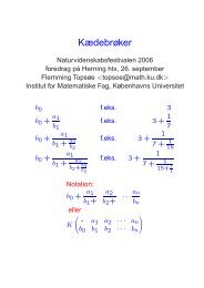
Figure 3: The price of the down-<strong>and</strong>-out call option for dividends D1 = D2 = 1 paid<br />
at times τ1 = T /3 <strong>and</strong> τ2 = 2T/3, computed by using the approximative numerical<br />
integration method (solid) <strong>and</strong> the Crank-Nicolson scheme (dashed) with very small step<br />
sizes.<br />
<strong>and</strong> so it only remains to compute P(t,St;K,σ,τ1,τ2) by evaluating one-dimensional<br />
integrals of the function P(τ1,g1(·);K adj<br />
1 ,σ adj<br />
1 ).<br />
For N > 2, we just continue this procedure recursively: at the kth step, k =<br />
S<br />
1,... ,N, compute an approximation of the time-τN−k price P(τN−k,St;K,σ,τN−k+1,... ,τN)<br />
by integrating P(τN−(k−1),g N−(k−1)(·);K adj<br />
k−1 ,σadj<br />
k−1 ). By convention, Kadj 0<br />
σ adj<br />
0 = σ, <strong>and</strong> τ0 = 0. Adjust the strike to<br />
K adj<br />
k := K +<br />
N�<br />
j=k+1<br />
<strong>and</strong> choose the adjusted volatility σ adj<br />
k such that<br />
<strong>and</strong> iterate.<br />
e r(T −τj) Dj = K adj<br />
k−1 + er(T −τk+1) Dk+1<br />
P(τN−k,St;K,σ,τN−k+1,... ,τN) = P(τN−k,St;K adj<br />
k ,σadj<br />
k ),<br />
= K,<br />
Figure 3 compares the price computed with the described approximative method<br />
to the result from the Crank-Nicolson scheme with very small step sizes. We consider<br />
the case N = 2 with dividends D1 = D2 = 1 paid at times τ1 = T/3 <strong>and</strong> τ2 = 2T/3.<br />
The approximation works nicely — relative errors are in the order of 0.1%-1%,<br />
10
except very close to the barrier, where the relative errors are larger. Running the<br />
approximative method takes only 0.05 seconds, so it is a fast alternative to the<br />
Crank-Nicolson method.<br />
6 Conclusion<br />
We described an extension of the method presented in Haug et al. (2003) for pricing<br />
the down-<strong>and</strong>-out call option in the Black-Scholes model when the underlying pays<br />
a discrete, deterministic cash dividend. The calculations above can be performed<br />
in exactly the same way for all the other single-barrier options (down or up, call or<br />
put, in or out). The method is also valid for one-touch options <strong>and</strong> similar variants.<br />
Knock-out options with rebates are also straightforward to h<strong>and</strong>le — one can use<br />
the same decomposition as for pricing in the no-dividend case — write the contract<br />
as a sum of the corresponding knock-out option without the rebate <strong>and</strong> a digital<br />
knock-in contract, see Poulsen (2006, Section 6.1). The method is benchmarked<br />
against solving the pricing PDE with a Crank-Nicolson scheme — as expected, our<br />
proposed method was significantly faster.<br />
We also described an approximation method in the case of multiple dividends<br />
for the down-<strong>and</strong>-out call option. Unfortunately, the same approach does not seem<br />
to be feasible for the other single barrier options — in this case, we are still limited<br />
to trees or finite difference schemes. Luckily, the case of multiple dividends is not<br />
paramount in practice — the vast majority of traded barrier options have expiries<br />
shorter than three months <strong>and</strong> dividends are usually paid less frequently than that.<br />
References<br />
Beneder, R. & Vorst, T. (2001), <strong>Options</strong> on Dividend Paying Stocks, in ‘Proceedings<br />
of the International Conference on Mathematical Finance’, World Scientific,<br />
pp. 204–217.<br />
Björk, T. (2004), Arbitrage Theory in Continuous Time, 2nd edn, Oxford University<br />
Press.<br />
Bos, R., Gairat, A. & Shepeleva, A. (2003), ‘Dealing with discrete dividends’, Risk<br />
(January), 111–112.<br />
11
Chriss, N. A. (1997), Black-Scholes <strong>and</strong> Beyond: Option Pricing Models, McGraw-<br />
Hill.<br />
Duffy, D. J. (2004), ‘A critique of the Crank-Nicolson scheme strengths <strong>and</strong> weak-<br />
nesses for financial instrument pricing’, Wilmott Magazine (July), 68–76.<br />
Engelmann, B., Fengler, M., Nalholm, M. & Schwendner, P. (2007), ‘Static versus<br />
Dynamic Hedges: An Empirical Comparison for <strong>Barrier</strong> <strong>Options</strong>’, Review of<br />
Derivatives Research 9, 239–264.<br />
Frishling, V. (2002), ‘A discrete question’, Risk (January), 115–116.<br />
Haug, E. G., Haug, J. & Lewis, A. (2003), ‘Back to Basics: a New Approach to the<br />
Discrete Dividend Problem’, Wilmott Magazine (September), 37–47.<br />
Mahayni, A. & Suchanecki, M. (2006), ‘Produktdesign und Semi-Statische Ab-<br />
sicherung von Turbo-Zertifikaten’, Zeitschrift für Betriebswirtschaft 76, 347–<br />
372.<br />
Østerby, O. (2008), ‘Numerical solution of parabolic equations’. Lecture<br />
notes, Department of Computer Science, University of Aarhus. URL:<br />
http://www.daimi.au.dk/∼oleby/notes/tredje.pdf.<br />
Poulsen, R. (2006), ‘<strong>Barrier</strong> <strong>Options</strong> <strong>and</strong> Their Static Hedges: Simple Derivations<br />
<strong>and</strong> Extensions’, Quantitative Finance 6, 327–335.<br />
Wilkens, S. & Stoimenov, P. A. (2007), ‘The pricing of leverage products: An<br />
empirical investigation of the German market for ‘long’ <strong>and</strong> ‘short’ stock index<br />
certificates’, Journal of Banking <strong>and</strong> Finance 31, 735–750.<br />
Wilmott, P. (2006), Paul Wilmott on Quantitative Finance, 2nd edn, John Wiley<br />
& Sons.<br />
Wong, H. Y. & Chan, C. M. (2008), ‘Turbo warrants under stochastic volatility’,<br />
Quantitative Finance 8, 739–751.<br />
12