Co-channel interference limitations of OFDM communication ... - KIT

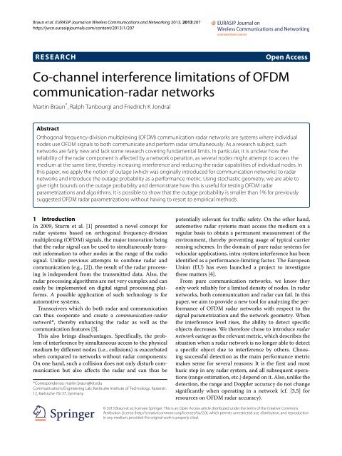
Braunetal. EURASIPJournalonWirelessCommunicationsandNetworking2013,2013:207http://jwcn.eurasipjournals.com/content/2013/1/207RESEARCHOpenAccessCo-channelinterferencelimitationsofOFDMcommunication-radarnetworksMartinBraun * ,RalphTanbourgiandFriedrichKJondralAbstractOrthogonalfrequency-divisionmultiplexing(OFDM)communication-radarnetworksaresystemswhereindividualnodesuseOFDMsignalstobothcommunicateandperformradarsimultaneously.Asaresearchsubject,suchnetworksarefairlynewandlacksomeresearchcoveringfundamentallimits.Inparticular,itisunclearhowthereliabilityoftheradarcomponentisaffectedbyanetworkoperation,asseveralnodesmightattempttoaccessthemediumatthesametime,therebyincreasinginterferenceandreducingtheradarcapabilitiesofindividualnodes.Inthispaper,weapplythenotionofoutage(whichwasoriginallyintroducedforcommunicationnetworks)toradarnetworksandintroducetheoutageprobabilityasaperformancemetric.Usingstochasticgeometry,weareabletogivetightboundsontheoutageprobabilityanddemonstratehowthisisusefulfortestingOFDMradarparametrizationsandalgorithms.Itispossibletoshowthattheoutageprobabilityissmallerthan1%forpreviouslysuggestedOFDMradarparametrizationswithouthavingtoresorttoempiricalmethods.1 IntroductionIn 2009, Sturm et al. [1] presented a novel concept forradar systems based on orthogonal frequency-divisionmultiplexing(OFDM)signals,themajorinnovationbeingthat the radar signal can be used to simultaneously transmitinformation to other nodes in the range of the radiosignal. Unlike previous attempts to combine radar andcommunication (e.g., [2]), the result of the radar processingis independent from the transmitted data. Also, theradarprocessingalgorithmsarenotverycomplexandcaneasily be implemented on digital signal processing platforms.A possible application of such technology is forautomotivesystems.Transceivers which do both radar and communicationcan thus cooperate and create a communication-radarnetwork a , thereby enhancing the radar as well as thecommunicationfeatures[3].This also brings disadvantages. Specifically, the problemofinterferencebysimultaneousaccesstothephysicalmedium by different nodes (i.e., collisions) is exacerbatedwhen compared to networks without radar components:On one hand, such a collision does not only disturb communicationbut also affects the radar and can thus be*Correspondence:martin.braun@kit.eduCommunicationsEngineeringLab,KarlsruheInstituteofTechnology,Kaiserstr.12,Karlsruhe76137,Germanypotentially relevant for traffic safety. On the other hand,automotive radar systems must access the medium on aregular basis to obtain a permanent measurement of theenvironment, thereby preventing usage of typical carriersensingschemes.Inthedomainofpure radarsystemsforvehicularapplications,intra-systeminterferencehasbeenidentifiedasaperformance-limitingfactor.TheEuropeanUnion (EU) has even launched a project to investigatethesematters[4].From pure communication networks, we know theyonly work reliably for a limited density of nodes. In radarnetworks, both communication and radar can fail. In thispaper,weaimtoprovideanewtoolforanalyzingtheperformanceof OFDM radar networks with respect to thesignal parametrization and the network geometry. Whenthe interference level rises, the ability to detect specificobjects decreases. We therefore chose to introduce radarnetworkoutageastherelevantmetric,whichdescribesthesituationwhenaradarnetworkisnolongerabletodetecta specific object due to interference by others. Choosingsuccessful detection as the main performance metricmakes sense for several reasons: It is the first and mostbasic step in any radar system, and all subsequent operations(rangeestimation,etc.)dependonit.Also,unlikethedetection, the range and Doppler accuracy do not changesignificantly when operating in a network (cf. [3,5] forresourcesonOFDMradaraccuracy).©2013Braunetal.;licenseeSpringer. ThisisanOpenAccessarticledistributedunderthetermsoftheCreativeCommonsAttributionLicense(http://creativecommons.org/licenses/by/2.0),whichpermitsunrestricteduse,distribution,andreproductioninanymedium,providedtheoriginalworkisproperlycited.

Braunetal. EURASIPJournalonWirelessCommunicationsandNetworking2013,2013:207http://jwcn.eurasipjournals.com/content/2013/1/207Page2of16A common characteristic of vehicular-based networksis high node mobility, which causes the geometrical configurationof nodes to change rapidly - and sometimesalsounpredictably.Sinceananalyticaldescriptionofthesecomplex spatial fluctuations is difficult, an exact modelingand analysis are not appealing. A remedy to thisproblem is given by the stochastic geometry framework[6-10], which models the node locations as a realizationof a point process, thereby essentially accounting for thespatial dynamics of the network. In this work, we willapply stochastic geometry tools to model the interfererlocations. The chosen approach will be instrumental fordetermining the outage probability of such an OFDMradar network given the physical parameters and providingadefinitiveansweronhowmanyparticipantsmaypartakein such a network before the radar system becomesunreliable. Most importantly, we can provide analyticalbounds for the probability of a radar outage. At low outageprobabilities, which is typically the targeted region ofoperation in car-safety applications, these bounds coincidewiththeexactoutageprobability.Thisisasignificantadvantage over current evaluation methods, which canincludetime-consumingsimulations,raytracingsetups,orcostlymeasurements.Using these bounds, we now have an objective metricto analyze various aspects of OFDM radar networks. Wegive two application examples of our bounds: the qualityof the target detection in a multi-target environmentand an answer on how the sub-carrier spacing affects theoutageprobability.This paper is structured as follows: Section 2 brieflydescribes the OFDM radar processing used here. Thesystem model for OFDM radar networks and how interferenceishandledarediscussedinSection3.In the next two sections, we recapitulate all the basicsof OFDM radar networks and clarify which assumptionsaremade.ThenewresultsarederivedinSection4,wherewe obtain analytical bounds on the outage probability ofradarnetworks,whicharefurtherverifiedbysimulations.With these results, we will give a discussion on how thisaffects the OFDM radar system in Section 5. Section 6concludes.1.1 PreviousresearchThe topic of mutual interference between radar systemshas recently become a focus of research due to the popularizationofvehicularradarsystems.ThepreviouslycitedEU research project MOSARIM [4] is an example of howrelevantthistopichasbecome.Radar interference has been researched both analyticallyand empirically. Brooker [11] provides a very thoroughanalysisofinterferenceinautomotiveradarsystemsat77and94GHz;hismetricofchoiceistheprobabilityofinterference. Brooker argues that in case of interference,radar systems cease to work and interference-avoidancetechniques must be introduced. This is not a suitablemetric for OFDM radar systems (and possibly for anyradarsystemwheretheinterferingradarsignalsappearasadditionalwhitenoise).Goppelt et al. chose the probability of ghost targetdetection as a figure of merit [12]. However, their resultscannot be generalized to OFDM radar, as the derivationsare specific to FMCW radar (despite being a commonlyapplied waveform, OFDM is rarely considered forradar networks). They also lack a random modeling ofthe interfering signal’s attenuation. Similarly, the analysisof Oprisan et al. [13] is also very specific to certainwaveforms.In general, current research focuses on interferenceavoidanceandmitigationtechniques,whichisexemplifiedby the results from the MOSARIM project, e.g., [14].Here, OFDM is in fact considered as a method to copewithmutualinterference,butfurtheranalysisisnotgiven.One suggestion to handle interference instead of avoidingit is given in [15], which is also the only publicationwhich directly researches interference in OFDM radarnetworks. The paper suggests an interference mitigationtechnique but only for the very specific scenario of onesingleinterferer.The difficulty of limiting the scope to a single interfereris also identified by Hischke [16]. He introduces a veryuseful quantity: The distribution of signal to interferenceplus noise ratio (SINR) as cause of mutual interference,as a function of the spacing between vehicles, from agivengeometry.Theresultsarederivedfromsimulations,though,emphasizingtheneedforananalyticalsolution.The importance of simulations is underlined by thework of Zwick et al. [17], who have done considerablework in the research of mutual radar interference. Theirapproach is empirical in nature and consists of elaboratesoftware tools packaged under the name Virtual Drive[18]. The results generated are highly useful but emphasizethe fact that highly sophisticated simulations are theonly means to research radar networks, motivating thederivationofanalyticalsolutions.In general, there has been little effort to create a ‘fundamentalradar network theory’, analogous to what informationtheory is for communication networks. Hischke’sapproach seems the most promising in this respect: If aprobabilitydistributionoftheSINRcouldbederivedforagiven radar interferer density, this would allow a stochasticanalysisoftheinterfererproblem.Moreimportantly,itwould ground the research on radar networks with theoreticalresults and provide benchmarks for the empiricalresults - at this point, there is no theoretical bound fortheperformanceofradarnetworks.Thispaperaimstobethefirststeptowardatheoreticalunderstandingofradarsoperatingundermutualinterference.

Braunetal. EURASIPJournalonWirelessCommunicationsandNetworking2013,2013:207http://jwcn.eurasipjournals.com/content/2013/1/207Page3of16Stochastic geometry as a tool for research on vehicularnetworkshaspreviouslybeensuggestedin[19],whichsuggestsitssuitabilityinthiscontext.2 OFDMradarsignalprocessingprinciplesIn the following, we present a very brief introduction toOFDMradar b .2.1 NomenclatureForeveryradarmeasurement,oneOFDMframeistransmitted.ItconsistsofMconsecutiveOFDMsymbols,withN active sub-carriers. Such a frame is represented by thetransmit matrix F Tx ∈ C N×M , using the notation introducedin [20]. Every column of this matrix represents anOFDM symbol, every row a sub-carrier. The elements(F Tx ) k,l (k = 1, . . .,N, l = 1, . . .,M) are symbols from acomplexmodulationalphabet(e.g.,QPSK).When transmitted, the sub-carriers are separated by asub-carrierspacingof f = 1/T,withT beingtheOFDMsymbol duration. As N carriers are transporting symbols,the signal bandwidth is B = Nf. Converting the matrixinto a discrete-time signal is done using the inverse fastFourier transform on the columns of F Tx . The transmitsignal is extended by a cyclic prefix of duration T G . Thisavoids inter-symbol interference but increases the totalOFDM symbol length to T O = T + T G . All relevantparameters for the OFDM radar transmitter are listed inTable1(thesevaluesarediscussedinSection3.5).Leaving aside synchronization and equalization, receivingOFDM signals is the exact same procedure as thetransmission, only in inverse order. The samples correspondingto the cyclic prefix are discarded, and the samplesare processed with a fast Fourier transform (FFT).EveryFFToutputisthenassignedtoacolumnofamatrixF Rx whichrepresentsthereceivedsignal.2.2 OFDMradarfundamentalsTo extend an OFDM transceiver into a radar system, itmust be made sure that during the transmission of everyOFDM frame, the receiver is active synchronously, i.e.,Table1 RelevantparametersofanOFDMtransmitterParametersymbol DescriptionExamplevaluef Sub-carrierspacing 90.9kHzT = 1 f OFDMsymbolduration 11µsT G Cyclicprefixduration 1.375µsT O TotalOFDMsymbolduration 12.375µsN Numberofactivesub-carriers 1,024(forU = 1)M OFDMsymbolsperframe 256f c centerfrequency 24GHzP Tx Transmitpower 20dBmtransmitterandreceiverusethesamelocaloscillatorand,derived from this, an identical clock (this setup describesmonostatic radar systems). This ensures that the transmittedsignal is delayed at the receiver by the round-trippropagation time of the electromagnetic wave wheneverit is scattered back to the original node from a radar target.If the target is moving relative to the radar system,this causes a Doppler shift which appears as a frequencydeviationofthereceivedsignalrelativetothetransmittedsignal.Using the matrix notation, it is useful to consider theform of a receive matrix F Rx given a transmit matrix. ForH reflectingtargets c ,thereceivematrixhastheform[20]H−1∑(F Rx ) k,l = (F Tx ) k,l ·b h e j2πlT Of D,he −j2πτhkf e jϕ h+(˜Z) k,l ,h=0whichcontainsthefollowingelements:• b h istheattenuationofthesignalreflectedfromtheh-thtarget;thisincludesbothfreespacepathlossanddifferentreflectivitycharacteristics(i.e.,radarcrosssections).• ϕ h isarandomphaseshift.• TheDopplershiftcausesafrequencyoffset2vf D,h = f rel,h C (v rel,h beingtherelativespeedofthec 0h-thtarget,c 0 thespeedoflight).WeassumethebandwidthofthesignaltobemuchsmallerthanthecenterfrequencyB ≪ f c ,sowecanapproximateanidenticalDopplershiftonallsub-carriers.Afrequency-shiftofonelineofF Tx isequivalenttomultiplyingitwithacomplexsinusoide j2πlT Of D,h .• Theround-tripdelay τ h = 2r hc 0(withr h beingtherangeoftheh-thtarget)causesaphaserotationofthereceivedsymbolsdependingonthesub-carrierfrequency,e −j2πτ hkf .• Additionally,thereiswhiteGaussiannoise(WGN),whichisrepresentedbythematrix ˜Z.The matrix F Rx still contains the modulation symbolsfromtheoriginaltransmission.Theseareirrelevanttotheradar processing but can be eliminated from Eq. (1) byelement-wise division with the (known) transmit matrix,resultingintheradarprocessingmatrix(1)(F) k,l = (F Rx) k,l(F Tx ) k,l(2)=H−1∑h=0b h e j(2π(lT Of D,h −kτ h f ) + ϕ h ) + (˜Z) k,l(F Tx ) k,l} {{ }=Z. (3)For phase-shift keying (PSK) modulation schemes, thenoise ˜Z retains its statistical properties after the division

Braunetal. EURASIPJournalonWirelessCommunicationsandNetworking2013,2013:207http://jwcn.eurasipjournals.com/content/2013/1/207Page4of16[20], as the phase of circular complex Gaussian randomvariables is uniformly distributed and thus has the sameprobability distribution after the division. The elements(Z) k,l ofZarethusstillrealizationsofaWGNprocesswithzeromeanandvariance σ 2 N .Now, the radar estimation problem can be expressed asa problem of spectral estimation. An OFDM radar algorithmbased on Eq. (3) must consist of at least two steps:(1) estimating the number H of sinusoid-pairs and (2)identifying their frequencies, which then translate intodistancesandrelativevelocities.For one-dimensional signals, the optimal way to identifysinusoids in white noise is the periodogram [21].Wethereforeextendtheperiodogramtotwodimensions,accounting for the different signatures of the row- andcolumn-wiseoscillations,resultingin∑Per(n,m)=∣(N Per −1 MPer −1k=0∑l=0lm−j2π(W) k,l (F) k,l eM Per)∣kn ∣∣∣∣2j2πeN Per .The dimensions of this 2D periodogram can be chosenlarger than those of F, N Per > N, M Per > M,which can be achieved by zero-padding F. This interpolatesthe periodogram, resulting in a smaller quantizationerror. The matrix W is a real tapering window matrix,the choice of which is outside the scope of this work d ;unless stated otherwise, we choose a boxcar window((W) k,l = 1).Figure 1 shows an example of such a periodogram withfivetargetsandmatrixdimensionsN Per =4N,M Per =4M.(4)Every pair of sinusoids in F manifests as a single peakwithitscenteratPer(m,n).Iftheperiodogramhasapeakatindices ( ˆm, ˆn),thiscorrespondstoatargetat[5]ˆr = c 02fˆnN Perand ˆv rel = c 02f C T OˆmM Per. (5)Whenamaximumdistanceandrelativespeedisknown,wecalculatemaximumindices ˆm, ˆnas⌈ ⌉vrel,maxM max = ·2f C T O M Per , (6)N max =c 0⌈rmaxc 0·2fN Per⌉. (7)BecausetheDoppler(unliketherange)canbebothnegativeand positive, we thus constrain the index ranges ofPer(n,m) to 0 ≤ n ≤ N max − 1 and −M max ≤ m ≤M max −1,therebycroppingtheperiodogramtoasmallersize (2M max +1) ×N max .The choice of N max and M max is relevant to the estimationprocess: Of course, they should not be chosen toosmall,asvalidtargetsmightnotbedetected,butchoosingthemtoolargeleadstoanincreasedfalsealarmrate.On a separate note, the threshold depends on the noisepower, which, as we explain in Section 3.3, is unknownforeveryreceivedframeandthusmustbeestimated.Thesimplestwaytodothisistochoosearowwithindexn 0 >N max andestimatethevarianceofthisrow,ˆσ 2 N = 12M max +1M∑max −1m=−M maxPer(n 0 ,m), (8)100−3580−40Distance (m)6040−45−50Received power (dBm)20−55−600−40 −20 0 20 40Relative speed (m/s)Figure1ExampleofaperiodogramPer(n,m)withH = 5,alltargetshavingdifferentradarcrosssection,range,andDoppler.

Braunetal. EURASIPJournalonWirelessCommunicationsandNetworking2013,2013:207http://jwcn.eurasipjournals.com/content/2013/1/207Page5of16which we take as a maximum likelihood estimate for thenoisepowergivenasinglerowoftheperiodogram.2.3 TargetdetectionandfalsealarmrateHaving calculated the periodogram, the next step is toidentifypeakswithintheperiodogramandtoreturnalistof targets, including their ranges and relative velocities.Wecallthisprocesstargetdetection.Themajorityofdetectionalgorithmsrelyonathresholdto separate noise from valid signal peaks. This thresholdis determined from the noise power as well as from therequired false alarm rate. It is commonly desired to keepthe false alarm rate at a constant level p F . This rate is theprobabilitythatanyoftheN max · (2M max +1)binsexceeda threshold θ. The noise in the periodogram is exponentiallydistributed with cumulative density functionF(x) = 1−e − xσN 2 ,solvingfor θ thereforeyieldsathresholdθ = σN 2 ·ln(1 − √ Nmax·(2Mmax+1) 1 −pF ). (9)} {{ }cWe abbreviate this ‘safety factor’ with c.Forthefollowingderivations,theassumptionismadethatatargetisalwaysdetectedwhenitscorrespondingpeakinPer(n,m) is larger than θ e . For a given distance r to thetargetandradarcrosssection(RCS) σ RCS ,wecancalculatethe peak value of the periodogram by applying the pointscatterapproximation([22],Chap.2),whichstatesthatthereceivedreflectedpowerisP Rx = P TxGc 2 0 σ RCS(4π) 3 f 2 . (10)r4cHere, G is the combined antenna gain of transmit andreceivepaths.As the transmit matrix has unit power, E{|F Tx | 2 k,l } = 1,the division (2) does not change the power, E{|F| 2 k,l } =E{|F Rx | 2 k,l } = P Rx. The periodogram finally shifts theentire power into a single bin, leaving the noise powerunchanged. Assume the bin index for a target is n 0 , m 0 ,andnonoiseispresent,thepeakvalueoftheperiodogrambecomesP peak = Per(n 0 ,m 0 ) = P Rx ·NM. (11)Withnoise,P max isarandomvariable,P peak = ∣ √ P Rx ·NM +z∣ 2 , (12)where z is complex, Gaussian distributed with the varianceσ 2 N .We simplify the following analysis by approximatingP max withitsexpectedvalue,givenacertainvariance:P peak ≈ E[max{Per(n 0 ,m 0 )}] = P Rx ·NM + σ 2 N . (13)We can justify the approximation by noting that thefactorNMisaverylargevaluefortypicalsetupsandthereforeP Rx · NM ≫ σN 2 when the interference is low. Onlywhenthenoisepowerbecomestoolarge(e.g.,whenthereis a very high number of interferers, see the followingsection), this approximation becomes inaccurate. In thisregion,aradarsystembecomeshighlyunusableanyway.3 RadarnetworksetupThe previous section discussed the operation of a singleOFDM radar unit. The next step is to describe howthesesystemsworkinamulti-userenvironment.Furthermore,weintroducetheconceptofoutageinOFDMradarnetworks, which will become the basis of further analyses.When designing an OFDM radar network, we mustmake sure to satisfy the assumption that all interferencecan be modeled as AWGN (this becomes relevant for thederivationsinSection4).3.1 Time-slottedmulti-useraccessWhen two OFDM signals interfere, we must distinguishtwo cases: synchronous and asynchronous interference.In the former case, all nodes start transmitting simultaneously,whereas in the latter case, both transmitters maytransmit at any given time. This second case is far worse,as the interfering OFDM signal would appear to have adifferent OFDM symbol duration, and its energy wouldrandomly leak across sub-carriers. This causes additionalproblems, which are avoided by enforcing simultaneousmediumaccess.We therefore postulate the following type of multi-useraccess,whichconcurswiththesystemproposedin[23]:• Accesstothemediumcanonlyhappenatthebeginningofatimeslot,whichisknowntoallnodes.• MediumaccessisallowedononeofU logicalchannels(asdemonstratedinFigure2).EverychannelmayonlyutiliseasubsetoftheOFDMsub-carrierswhichconsistofeveryU-thsub-carrier,startingatsub-carrieru,whereu denotesthechannelnumber.NotethatthischangestheOFDMprocessingonlyinawaysuchthatthesub-carrierspacingisincreasedbyU andthenumberofrowsinFisreducedby1/U.Consequently,thepowerperactivesub-carrierisincreasedbyU,inordertomaintainthesametransmitpower.• Everynodemayrandomlyaccessanychannelstartingatthebeginningofanytimeslotwithprobabilityp Tx .WhilethisallowsnosophisticatedMAC(e.g.,

Braunetal. EURASIPJournalonWirelessCommunicationsandNetworking2013,2013:207http://jwcn.eurasipjournals.com/content/2013/1/207Page6of16Sub-carrier index76543210. . .T GT o2T o 3T oFigure2Examplesformediumaccess:Therearetwochannels(U = 2).Inthefirsttimeslot,anodeaccesseschannel0,whichutilizestheevensub-carriers.Inthesecondslot,twonodesaccesschannelsu = 0andu = 1,respectively.Finally,twonodesaccessthemediumonthesamechannel,causingacollision.. . .tthroughback-offmechanismsorsimilarcollisionavoidancetechniques),itallowsaradarsystemtoaccessthemediumatregularintervals,whichisarequirementforsafety-ensuringradarsystems.Having multiple channels in the frequency domainallows for anOFDMA-like multiple access scheme;if twoor more nodes access the medium in the same time slot,theyonlycollideiftheyusethesamechannel.From a practical point of view, stipulating synchronousaccess by time slots requires a global clock. This could beprovided by global positioning system (GPS) f . The guardintervalT G mustthenbechosenlargeenoughtoallowforclockinaccuraciesanddifferentsignalarrivaltimesduetodifferentdistancestotheotherradartransmitters.If clocks differ too much between nodes, minor interferencecan also be caused by nodes which have chosena different channel u. For this work, we accept a certaininaccuracyofthemodelandassumeperfectorthogonalitybetween channels, as we focus on the definition of radarnetworkoutageandhowtoderiveit.3.2 RadarnetworkoutageIncommunicationnetworks,outageisacommonconceptto describe the case where an ongoing transmission failsto achieve a given rate. Goldsmith [24] defines outage asthe event where SINR (the ratio of received signal powertothesumofnoiseandinterferencepower)dropsbelowacertain value due to slowly varying, random channel conditions.We can directly transfer this notion to a radarnetworkbydefiningoutageasthecasewhenthereflectedpower at the receiver drops below a certain thresholddue to the interference created by the randomly locatednodes.For a meaningful analysis, we define a reference targetas a fixed object at range r Ref and with a radar crosssection σ RCS,Ref . These values are chosen depending onthe application at hand (see Section 3.5). Whether anobject is detected or not depends on the received power,which is calculated from (10) using the reference targetspecifications,P Rx,Ref = P TxGc 2 0 σ RCS,Ref(4π) 3 fc 2 . (14)r4 RefThe outage definition is therefore the same for anyobject with the same backscattered power P Rx,Ref . Theperformance of an OFDM radar network is completelydefinedbythedetectionofthistarget.From Section 2.2, we know that detection is only possibleif the peak in the periodogram corresponding to thetarget has a maximum value larger than the threshold θ,whichisarandomvariableasweconsidertheinterferencepower to be random. The outage probability is thereforetheprobabilitythatthispeakissmallerthan θ,p out = Pr [ P peak < θ ] (15)(13)≈ 1 −p D . (16)By applying the approximation (13), outage probabilityiscomplementarytothedetectionprobabilityp D .This also implies that multi-path propagation of theradar signal does not affect the outage probability andis thus not considered here. A multi-path backscatteringmight produce additional peaks in the periodogramwhichdonotcorrespondtotruetargets,butthisisacommonproblem of all radar systems and must be treateddownstreamintheprocessingchain.3.3 InterferencemodelTo model the interference, we use a stochastic model forthe interferer geometry. The reference node is located atthe origin of a plane. The positions of the other, interfering,nodesfollowastationarytwo-dimensionalPoissonpoint process (PPP) with density λ g . Figure 3 illustratessuchascenario.AformalintroductionofthespecificPPPfollowsinSection4.3.

Braunetal. EURASIPJournalonWirelessCommunicationsandNetworking2013,2013:207http://jwcn.eurasipjournals.com/content/2013/1/207Page7of16d refG( )Figure3Anexampleofthenetworktopology:thereferencenode(center)istryingtodetectareferencetarget(circle).Othersystems(squares)arerandomlydistributedandcaninterfere.The reason we choose to model the geometry by a PPPis because not only does this provide us with the mathematicaltools to analyze such a scenario but also becausethe main application we have in mind for radar networksis for vehicular technology, where mobility causes a highamount of ‘spatial randomness.’ Such a spatial model hasbeen shown to properly capture these random spatialdynamicsaffectingtheinterference[25].We emphasize that all nodes represented by this PPPare OFDM transmitters of the same type as the referencenode. Because of the homogeneous setup, the results forthe reference node are representative for all other nodesaswell.As this is a radar system, we need to be able to determinetheazimuthφ ofthetargetsaswellastherangeandDoppler. How the radar system implementation solvesthis problem is irrelevant for this work, what matters isthat the angular resolution results in a receiver directivitywhich can be expressed as azimuth-dependant gainG(φ). For the transmitters, we assume that they emitomnidirectional so they can communicate with all othernodes.Atthispoint,wehavealltheknowledgerequiredtocalculatetheoutageprobabilityforanOFDMradarnetworkwith a given network density λ. To recapitulate, the reasonfor outage is that whenever the reference node triesto obtain a radar image, a number of interferers might bealsotransmitting.Thisincreasestheinterferencelevelandthusthethreshold θ.To show that the network setup still allows the usageof the radar processing from Section 2.2, we must showthatthetotalinterferenceisadditivewhiteGaussiannoise(AWGN). Conditioning on a certain spatial configuration,assume we have I interferers, with F Ix,i being thetransmit frame of the i-th interferer. The noise matrixZ now does not only contain the receiver noise butalso energy from the interfering transmit symbols. Byassuming synchronous interference (see Section 3.3), wemay analyze the total noise matrix element-wise, whichthenbecomesI−1∑ √ (F Ix,i ) k,l(Z total ) k,l = Z k,l + bi e jϕ i. (17)(F Tx ) k,li=0Rememberthatthe (F Ix ) k,l arezeroforinterfererswhichuseadifferentchannelthanthereferencenode(assumingperfectorthogonality).On top of the receiver noise, we now have a sum ofcomplexvalueswithrandomamplitudeandphase;wecanmodel the latter as uniformly distributed within [0,2π).Theformerismodeledbyanexponentialpathloss,βb i = g iriα G(φ), (18)where r i is the distance to the origin, φ the azimuth andα > 2 the path loss exponent. β is a constant attenuationfactor,whichisassumedtofulfillβ = P Txc 2 0(4π) 2 f 2 C(19)in correspondence with free space path loss. g i is anoptional random small-scale power attenuation parameter(caused by fading) with distribution function F g (g) h ;we discuss the cases where g i = 1 (i.e., no fading),or i.i.d. exponentially distributed with unit mean(Rayleigh fading). This fading parameter covers multipathpropagation of the interference signals. A very similarmodelisalsodescribedin[19].Any fading type can be inserted, as long as its distributionfunction can be given. Here, Rayleigh fading waschosenasanexampleforafadingmodel,asitisapopularchoiceforthemodelingofwirelessfadingchannelsanditsprobability density function (pdf) is mathematically easytodescribe.

Braunetal. EURASIPJournalonWirelessCommunicationsandNetworking2013,2013:207http://jwcn.eurasipjournals.com/content/2013/1/207Page8of16In the special case where the modulation has constantamplitude (e.g., as in PSK) and the amplitude is Rayleighdistributed,Ztotal isasumofnormallydistributedrandomvariablesandthereforeisnormallydistributedbythecentrallimit theorem. For the more general case where theb i follow any distribution (in Eq. (18), we state that theydepend on the distance of the interferers to the referencenodeandarethusnot identicallydistributed),wemaystillrefertothecentrallimittheorem,whichstatesthatasmallnumber of summands (10 to 12) suffice for Z total to beapproximatelyGaussian([26],Chap.2).For the rest of this work, we will omit the index ‘total’anduseZtodescribethecompoundnoisewithtotaltwosidednoise power σN 2 + Ỹ, where Ỹ denotes the randomvariablerepresentingthetotalinterferencepower.3.4 ClutterWe have deliberately omitted a modeling of clutter, fortwo reasons: First, there are many different clutter models,and incorporating one specific model would makeour results less versatile. Second, the outage probabilityis a theoretical boundary depending on the specificationsof the reference target, and as such is unaffected byclutter.This approach is not unusual in vehicular radar applications,whereclutteriscommonlynottreateddifferentlythan other targets at the detector; an example would bethe detection of a road sign when intended targets areother vehicles. Both these objects register as a backscatteringobjectatthereceiver(andthereforeasapeakintheperiodogram).3.5 ParametrizationIn the case where we need to specify the parameters(e.g., for simulations), we use the values given in Table 1,which coincide with the parameters chosen in previouspublications [1,27]. These parameters are also discussedin[3],andresearchontheradaraccuracyforasinglenode(outsideofanetwork)hasbeendonethroughsimulationsin [5] and by measurements in [27]. They provide a rangeresolution of approximately 3.2 m, and a Doppler resolutionofapproximately2.5m,althoughsomemodificationsof the parametrization (e.g., other window matrices W)can degrade this value. For a detailed discussion on thechoiceoftheseparameters,wereferto[28].All other parameters relevant to the network setup arechosenasshowninTable2.The target parameters are chosen to work within avehicularscenario.Forthereceiver,thenoisefigureisonecompound value encompassing all non-idealities and distortionscaused by the amplifiers and the digital signalacquisition. The receiver noise power is then calculatedusing the given bandwidth (B = Nf = 93MHz) and atanoisetemperatureof290K.Table2 Radarnetworksetupr Refv rel,RefTargetparameters50m0m/sσ RCS,Ref 10m 2P Rx,Ref 10m 2d maxv rel,max300m150m/sN max 187M max 153NoisefigureThermalnoisepowerReceiverparametersNetworkparameters10dB−84.2dBmp F 0.01p Tx 0.1As for the network parameters, if we specify a time slotdurationof5ms,theaveragemediumaccessrateis20Hz,a typical value for automotive radar systems. The falsealarm rate is the targeted false alarm rate at the detector;in practical systems, tracking devices or similar systemswill further decrease the false alarm rate for practicalpurposes.Fortheantennagain,wedefinethewidthoftheantennabeam as φ 0 and use one of two different functions, eitheraconeshape,G cone (φ) = 1 |φ|

Braunetal. EURASIPJournalonWirelessCommunicationsandNetworking2013,2013:207http://jwcn.eurasipjournals.com/content/2013/1/207Page9of164 AnalyticalresultsToanalyticallycalculatetheoutageprobability,wefirstreiterateontheassumptionsandapproximationsmade.4.1 Assumptions• Thetotal,additiveinterferenceZismodeledbyWGN.This implies a clock synchronization as discussed inSection3.1,and thatthe datasentbythe individualinterferersare uncorrelated. Note that this is accurate foran OFDM radar system as described above; it merelyrequires the individual elements of Z to be i.i.d. Gaussiandistributed(cf.Section3.3) j .• Themediumaccesscanbedescribedbyatransmitprobabilityp Tx ,andatransmittingnodewillrandomlychooseoneofU logicalchannels,eachwithequalprobability(cf.Section3.1).• Theattenuationbetweeninterferingtransmittersandthereferencesystemismodeledbypathlossanda(random)fadingcoefficient,seeEq.(18).Thesetwoassumptionsmightbelessaccurateforsomespecific scenario but are the most sensible assumptions iftheOFDMradarsystemisnotspecifiedanycloser.• Nodesaredistributeduniformlyandindependently.This allows us to use the tools described in Section 4.3.It is motivated by the fact that due to the mobility of thenodes, their relative position changes all the time and isthusdifferentbetweentimeslots.4.2 Approximations• Sub-carriersarealwaysorthogonal,interferenceonadifferentchannelthusdoesnotaffecttheradarsystem.• AnidealradarsystemcanalwaysdetectthereferencetargetifP Rx ·NM +E [ |z| 2] > θ,i.e.,Eq.(13)isanequality.Thesearetheonlysimplificationsinthismodelwhicharedesigned to facilitate the derivation of analytical bounds.TheirinfluenceisdiscussedinSection5.2.4.3 StochasticmodelGiven the synchronized slotted medium access of thenodes, we consider the network in an arbitrarily chosenslot (snapshot). In this snapshot, the locations of thepotentially interfering nodes are given by the PPP withdensity λ, as already explained in Section 3.3. From Slyvniak’stheorem [6,29], it follows that the law of the PPP isnotchangedbyaddinganode.Duetothestationarity,thisnode can be placed in the origin without loss of generality.We will refer to this node as the reference node as itwillallowustomeasurethetypicalperformanceinsuchanetwork.Since the medium access is uncoordinated among thenodes,i.e.,eachnodeaccessesthemediumindependentlyofeachotherwithprobabilityp Tx ,wecanobtainthesetofinterfering nodes by independent thinning of the originalPPP[8].TheresultingpointprocessisagainPoissonwithdensityp Tx λ.We treat the sub-carriers chosen by the i-th node asmark attached to this node. Formally, if node i choosesthe u-th sub-carrier for transmission, we assign the marku i to this node. The small-scale channel fading experiencedbetween the i-th interferer and our reference nodeisdenotedbyanothermark,g i .Having introduced all relevant system parameters, wecan now formally define the set of interferers by thestationaryindependentlymarkedPPP := {(x i ,u i ,g i )} ∞ i=1 (22)of (spatial) density p Tx λ, where the x i denote the randominterfererlocations,andu i andg i arethemarksassociatedwithinterfereri.Notethat (x i ,u i ,g i ) ∈ R 2 ×U×R + ,whereU = {1, . . .,U}.Withoutlossofgenerality,weassumethatthereferencenode receives on the first channel, u = 1. Then, the suminterferencepowermeasuredatthereferencenode(intheorigin)isgivenbyY= ∑1 (ui =1) ·G(∠x i )g i ‖x i ‖ −α , (23)(x i ,u i ,g i )∈where ‖x i ‖ −α describes the large-scale path loss betweeninterferer location x i ∈ R 2 and the origin, and ∠x i theinterferer’sazimuth.Atthereceiver,thesuminterferenceissuperimposedbythermalnoiseofpower σ 2 N .Asshownpreviously,theinterferencenoisecanbeassumedtobeconditionallyAWGN.Consequently, the total noise is conditionally AWGN aswellwitha(random)powerequaltoỸ+σ 2 N .We must point out that Y is a normalized, unit-lessinterferencepowerterm,whichisintroducedforitsmathematicalutility.Ontheotherhand,Ỹincludesthephysicaleffects, such as frequency-dependence of the free spacepathloss.ConvertingonevalueintoanotherisdonebyỸ = Y ·Uβ. (24)Thefactor β playsthesameroleasinEq.(17).U isnecessarybecause the power on the individual sub-carriersis scaled by the same factor to retain a constant transmitpower.4.4 OutageprobabilityanalysisFromSection3.2,wehavethatp out = Pr [ P peak < θ ] . (25)

Braunetal. EURASIPJournalonWirelessCommunicationsandNetworking2013,2013:207http://jwcn.eurasipjournals.com/content/2013/1/207Page10of16In order to make use of stochastic geometry, we mustexpress this probability in terms of Eq. (23), which weachievebyinsertingEqs.(9),(13),and(24).Thisresultsinp out = Pr [ P Rx NM +UβY + σN 2 < (UβY + σ2 N )c] (26)⎡⎤= Pr ⎢⎣ Y ≥ 1 ((c −1) −1 P Rx NM − σ 2 ⎥UβN)⎦ . (27)} {{ }ωHence,computingp out requirestheevaluationofthetailprobability of Y (note that Eq. (27) assumes that c − 1 ispositive,butunlessp F iscloseto1,thisisalwaysthecase).Unfortunately, solving Eq. (27) directly is an intractableproblem;therefore,wepresentboundsinthefollowing:4.4.1 LowerboundTo obtain a lower bound, we make use of the dominantinterferer phenomenon which was originally introducedfor communication networks (see [7]), and adapt it to thecase of radar network outage. The idea is to divide theset of total interferers into the set of dominant and nondominantinterferers. Formally, these sets are defined as{}∣ d := (x i ,u i ,g i ) ∈ ∣1 (ui =1)G(∠x i )g i ‖x i ‖ −α ≥ ω(28)and{}∣ nd := (x i ,u i ,g i ) ∈ ∣1 (ui =1)G(∠x i )g i ‖x i ‖ −α < ω .(29)Notethat d ∩ nd = ∅.Accordingly,wedefine∑Y d := 1 (ui =1)G(∠x i )g i ‖x i ‖ −α (30)(x i ,u i ,g i )∈ dandY nd :=∑(x i ,u i ,g i )∈ nd1 (ui =1)G(∠x i )g i ‖x i ‖ −α , (31)where Y = Y d + Y nd . The intuition behind Eqs. (28) and(29)isthat d containsthoseinterferersthatdirectlycreateoutageindividually,while nd containsinterferersnotdirectlycreatingoutage.Theoutageprobabilityisthusp out = Pr[Y d +Y nd > ω]. (32)We can construct a simple lower bound by neglectingtheY nd term:p out ≥ p out,d := Pr[Y d > ω] (33)= Pr[ d ̸= ∅], (34)wheretheequalitystemsfromthefactthatthepresenceofonedominantinterfereralreadysufficestomaketheeventY > ω true. Since d is still a PPP, we have to computethe void probability of the Poisson distributed randomvariable | d |,i.e.,p out,d = 1 −exp(−µ), (35)wherethemean µcanbecalculatedusing[8]as∫µ = p Tx λ E [ ]1 (u=1) 1 (G(∠x)g‖x‖ −α ≥ω) dx (36)R∫2= p Tx λ Pr[u = 1]Pr [ G(∠x)g‖x‖ −α ≥ ω ] dxR 2 (37)= p ∫]TxλPr[g ≥ ω‖x‖α dx. (38)U R 2 G(∠x)Atthispoint,theboundonlydependsontheprobabilitydistribution of the fading. For the fading cases discussedinSection3.3,wecangivesolutionsfor µ:Purepathloss(g ≡ 1) Inthiscase,]Pr[g ≥ ω‖x‖α → 1 (G(∠x) ‖x‖≤) ) 1/α , (39)andtherefore,µ = 2p TxλU= p TxλU∫ π0∫ π0∫ ( ) 1G(φ) αω0( G(∠x)ωrdrdφ (40)( ) 2G(φ) αdφ. (41)ωRayleigh fading (g ∼ Exp(1)) Here, the probability isgivenby])Pr[g ≥ ω‖x‖α = exp(− ω‖x‖α , (42)G(∠x) G(∠x)andtherefore,weobtain µbysolvingµ = 2p ∫ π ∫ ∞)Txλrexp(− ωrα drdφ (43)U 0 0 G(φ)= 2p ∫ π ∫ ∞(Txλt α 2 −1 exp − ωt )dtdφ (44)αU 0 0 G(φ)= p Txλ(1U Ɣ + 2 ) ∫ π( ) 2G(φ) αdφ, (45)α ω0where Ɣ(·) is the gamma function. Hence, we obtain thelowerbound:p out ≥p out,d=1 −exp(− p TxλU ω− 2 α Ɣ(1 + 2 α) ∫ π0G(φ) 2 α dφ)(46)

Braunetal. EURASIPJournalonWirelessCommunicationsandNetworking2013,2013:207http://jwcn.eurasipjournals.com/content/2013/1/207Page11of16TheonlydifferencebetweentheRayleighfadingandthepath-loss-onlyscenarioisthe Ɣ ( 1 + 2 α)function,whichisnotpresentfornofading.Approximating the directivity At this point, the lowerbound still depends on an integral over G(φ). If G(φ) isknown,theintegralmaybesolvedanalytically.Otherwise(e.g.,iftheantennagainisonlygivenintabularform),theintegralmustbesolvednumerically.Wewillshowtheformercase for the cone-shaped antenna function G cone (φ)andRayleighfading,wherethelowerboundbecomesverysimple:(p out ≥ p out,d = 1 −exp − p Txλφ 0U ω− α 2 Ɣ(1 + 2 )).α(47)4.4.2 UpperboundBecauseboththedominantandnon-dominantinterfererscancauseoutage,wecanwritep out = Pr[Y d ≥ ω] +Pr[Y d < ω]Pr[Y nd ≥ ω]= p out,d + ( 1 −p out,d)Pr[Ynd ≥ ω], (48)wherethesecondequationstemsfromthefactthatdominantinterferersalwayscauseoutagewhenpresent.Weobtainanupperboundonp out byapplyingMarkov’sinequality[30],Pr[Y nd ≥ ω] ≤ 1 ω E[Y nd]. (49)We therefore focus on the first moment of Y nd : UsingCampbell’s theorem [6], we can compute E[Y nd ] as follows:⎡⎤∑E[Y nd ]=E⎣1 (ui =1)1 (G(∠x)g‖x‖ −α

Braunetal. EURASIPJournalonWirelessCommunicationsandNetworking2013,2013:207http://jwcn.eurasipjournals.com/content/2013/1/207Page12of161(a)p D0.5022.5 3 3.5Path loss exponentU = 1U = 8Figure5Simulatedresults(solidlines)andbounds(dashedlines)for λ = 10 −2 , φ 0 = π/2,andsinc-shapedantennagain.4too, the bound becomes less tight for higher interferencelevels.(b)(c)Figure4Simulatedresults(solidlines)andbounds(dashedlines)for α = 4, φ 0 = π/2,andvaryingnodedensities.(a)Cone-shapedantennafunction.(b)Sinc-shapedantennafunction.(c)Sinc-shapedantennafunction(outageprobability).bound for p D , and vice versa. We cannot only see thatthe bounds are correct but also that the upper boundis very tight and can be used as a good approximationof the actual detection probability. The tightness of theupper bound results from the fact that, especially at highdetection rates (which typically is the desired region ofoperation in practical car-safety applications), the ‘dominantinterferer’ effect outweighs the sum interferencecreated by the non-dominant interferers. This concurswithotherresearchusingstochasticgeometry[7,10].Figure5showsthesamesimulationbutwithavariationof α instead of λ. When α approaches 2, the overall interferenceincreases, as nodes from further away becomemore and more influential. We can observe that here,4.5.2 ModelrobustnessforrealestimatesThe previous simulation assumes perfect detection; i.e.,the reference target is guaranteed to be detected whenP peak > θ. More realistic simulations are required toverify if the model works with the signal processing presentedin Section 2 and the approximations shown inSection4.1.However, it is important to separate the detectionfrom the multi-target identification, which will be discussedin Section 5.2. A target identification systemhas to distinguish sidelobes from targets, handle thecase where targets are very close and have overlappingmain lobes, etc., and therefore is an additional sourceof errors. To simulate an OFDM radar system withoutintroducing multi-target-related errors, we create ascenario where everything except the reference targethas zero RCS, and the reference target is therefore theonly scatterer. The interferers only produce interferencenoise.The simulation works as follows: For every iteration, anumberofinterferers(andtheirpositions)ismodeledthesame way as in Section 4.5.1. The reference node, as wellaseveryactiveinterferernode,transmitanOFDMframe.ThesignalofthereferencenodeisattenuatedaccordingtoEq.(14)anddelayedby τ = 2 r Refc 0.Theinterferencesignalsare attenuated according to their azimuth and antennafunction as well as the path loss (with α = 4). To reducethe amount of random effects, no small-scale fading isappliedhere.All signals (reflected reference signal and all interferersignals) and the thermal noise are added up and passedto an estimator that works as described in Section 2.2.Weconfirmadetectionbycheckingthattheperiodogrambin corresponding to the reference target’s distance andDopplern 0 = r Refc 02fN Per (roundedtothenearestinteger)is larger than the threshold, Per(n 0 ,0) > θ. At everysimulationpoint,1,000iterationswererun.

Braunetal. EURASIPJournalonWirelessCommunicationsandNetworking2013,2013:207http://jwcn.eurasipjournals.com/content/2013/1/207Page13of1611p D0.9p D0.50.810 410 310 2Node densityFigure6Simulationoftheidealdetector(α = 4,cone-shapedantennafunction, φ 0 = π/2,U = 1,nofading).Thesolidlineshowsthesimulationresults,thedashedlinestheanalyticalupperandlowerbounds.10 1Figure6showsthesimulationresults.Notethatthesimulatedcurve again stays very close to the upper bound.This confirms that the approximation (13) is justified, asthe simulated curves from Figures 6 and 4 are very closetoeachother.Because this simulation omits all multi-target-relatederrors, it is called an ideal detector in the following.It is clear that such a detector cannot be implementedin reality, where there are many targets withnon-zeroRCS.5 ConsequencesfortheOFDMradarnetworkparametrizationAs an approximation for the outage probability, thebounds can be an extremely useful tool. The followingsection gives some practical examples of theirutility.5.1 NetworkfeasibilitystudyThemostobvioususeforthesenewmetricsisafeasibilitycheck of a given radar network to determine whether ornot a network would fulfill certain QoS requirements. Inthis case, we can take a set of system parameters and usetheboundsforthedetectionprobabilitytoseeiftheradarsystemisexpectedtoworkreliably.As an example, consider the results from Figure 4. Saythat we require a detection probability of 99% for safetyreasons, the node density cannot increase beyond λ =10 2.2 , which corresponds to one node per 158.5 m 2 onaverage. In a vehicular scenario, this corresponds to anaverageofonevehicleequippedwithanOFDMradarsystemevery 53 m for a lane width of 3 m, which seemsrealistic given that most likely, not all vehicles wouldbe equipped with such a radar system. For other nodedensities, the corresponding detection probability can beread from Figure 4. If the radar system must work witha specific detection probability with a higher node density,the parametrization can be changed in several ways:02040 60 80 100Distance of reference object r Ref120Figure7Detectionprobabilityoverdistanceofthereferenceobject. α = 3, λ = 10 −2 ,sinc-shapedantennagainwith φ 0 = π/2.Either the number of channels U is increased, or φ 0 isreduced.This also works the other way: given a node density λandaminimumdetectionprobability,whatisthesmallesttarget the radar can detect? We can calculate the detectionprobabilityfordifferentvaluesofPpeak toanswerthisquestion. Figure 7 shows p D as a function of r Ref (P peak isrecalculatedforeveryvalueofr Ref usingEq.(13),Eq.(14),and the values from Section 3.5). This time, the P Rx,Refis reduced instead of increasing the average interferencepower. We see this has a similar effect concerning thebounds.It is worth pointing out the analogy to the outagecapacityofcommunicationnetworks,whichisadataratethat can be achieved with a given probability. Here, atarget with peak amplitude P peak can be detected withprobabilityp D .So far, this could be achieved by simulations - althoughtime-consuming, the results would be very similar. Toshow the benefits of using the lower bound for p outas an approximation, we take our previous result (56)(p D ) pD0.150.10.0500p F= 0.05p F= 0.01p F = 0.0010.2 0.4 0.6 0.8 1Detection probability p DFigure8UsingthelowerboundfortheoutageprobabilitytocalculateEq.(58). α = 4,cone-shapedantennafunction,Rayleighfading.

Braunetal. EURASIPJournalonWirelessCommunicationsandNetworking2013,2013:207http://jwcn.eurasipjournals.com/content/2013/1/207Page14of16(cone-shapedantennafunction,Rayleighfading)andsolveitfor λ:−log(p D )Uλ(p D ) =p Tx φ 0 ω − α 2 Ɣ ( ). (58)1 +α2This allows us to first fix a tolerable detectionprobabilityandthenobtainamaximumnodedensityfromthat. Using (58), we can now plot the expected densityof successfully detecting nodes (p D · λ(p D )) as a functionof the required detection probability. Figure 8 shows thisvaluefordifferentvaluesofp F .This demonstrates how these simple bounds provide apowerfultoolforbenchmarkingthenetworkperformanceofanOFDMradarsystem.5.2 EvaluationofthedetectionperformanceSection 4.5 discussed how well an ideal detector wouldperform. This can be used as a benchmark for practicalimplementations.Todemonstratethis,thesimulationinSection4.5.2wasmodified to a more realistic scenario: First, every interfereris assigned a random RCS which obeys an exponentialdistributionwithpdfp(σRCS ) = 1−σ RCS¯σ RCSe¯σ RCS , σ RCS > 0.ThemeanRCSwaschosenas ¯σ RCS = 10m 2 .Next, the radar signal processing uses a modifiedCLEAN algorithm [31] to estimate Doppler and range ofall interferences and the reference target. This algorithmdetects the largest peak in the periodogram, estimatesrange and Doppler, and then subtracts the componentsfrom the periodogram caused by the estimated values.This process is repeated until the largest remaining peakis smaller than θ. To make sure peaks are not caused byresiduals during the subtraction process, peaks detectedwithin the main lobe of a previously detected target arediscardedduringtheprocess.Forlarge λ,theprobabilityofalargetargetbeingincloseproximity to the reference target increases, in which casethereferencetargetmightbeovershadowedandthereforenotdetected.p D10.80.60.410 4 10 310 2Node densityFigure9Simulationusingthecancelationalgorithm(α = 4,cone-shapedantenna, φ 0 = π/2,U = 1,nofading).Onlytheupperboundisdisplayed(dashedline).10 1The simulation results in Figure 9 confirm this (notethat we only consider detection of the reference target;the detection probability of the other nodes is not a usefulmetricastheirpositionsarerandom).Wecanidentifya significant reduction of the detection probability comparedtotheidealdetector,althoughitmustbenotedthatfor higher node densities, the detector is forced to handleseveralhundredclutterobjects(theinterferers),whichisadifficult task for radar systems in general. The root meansquare (RMS) error of the estimation was also measuredduring the simulations, but as a successful detection is aprerequisite of calculating an error, the RMS error constantlystays below 0.6 m for the range and below 0.6 m/sfortheDopplerestimation.UsingEq.(56),wecanquantifytheperformancereductionof the successive cancelation algorithm comparedto the ideal detector for a certain configuration. FromFigure 9, we inspect the situation for λ = 10 −3 and findthat at this density, we achieve a detection probability ofp D = 0.85.Toquantifythedetectorloss,wesolveEq.(46)for P Rx,ref and determine which reflected energy wouldcause the ideal detector to have the same detection probability(we use the upper bound as the value for the idealdetector):P Rx,detector = c −1NM( ( ) α)P Tx λφ 0 2Uβ + σ2Ulog(1 −p D ) N(59)Bycomparingthereceivedpowerwiththereflectedpowerofthereferenceobject,wemaydefinethedetectorlossasL = P Rx,detectorP Rx,ref. (60)ForthevaluesusedtocreateFigure9,weobtainareceivedpower of −127 dBm, or an 18-dB detector loss. Othermulti-target detection algorithms might achieve bettervalues, but we now have a practical limit for how goodsuchanalgorithmcanget.We emphasize that this benchmark is only valid for afixedscenario.5.3 Choiceofsub-carrierspacingIn Section 3.1, we introduce the possibility of using a carrierspacingmethod(U> 1)toallowmultipleuseraccessto the medium. This has two effects: first, it decreasesthechanceofacollision,asdifferentusersmayaccessthemediumondifferentlogicalchannels.Ontheotherhand,whenever a collision occurs, the influence of the interferingsignal is in fact worse than it were for U = 1, becausethesignalpowerperactivecarrierisincreasedbyafactorU. This requires a closer analysis on how the choice of Uaffectsthemulti-userperformance.

Braunetal. EURASIPJournalonWirelessCommunicationsandNetworking2013,2013:207http://jwcn.eurasipjournals.com/content/2013/1/207Page15of16Theseresultsprovideasimpleanswerforthis:considerEq. (46), where U appears twice: once in the PPP density(p Tx λ/U), and once in ω α. 2 The argument of the exponentialfunction therefore depends on U −( α 2 −1) . Because2α−1 > 0,theoutageprobabilitywillalwaysdecreaseforhigher U, and this can thus be chosen as large as externalconstraintspermit.6 ConclusionsIn this paper, we have suggested a novel figure of meritfor radar systems: the radar outage probability. This is ascalarvaluewhichdescribesthecapabilitytodetectaspecifictarget. It depends on the density of nodes and thewaveformparameters.More importantly, we could derive an asymptoticallytight bound, which provides an analytical expression ofradar systems without simulations or measurement campaigns(althoughempiricalmethodsareusedtoverifytheresults). As an example, we can calculate that the OFDMradarsystemsuggestedin[3]wouldhaveanoutageprobabilityof lessthan 1% for traffic densitiesbelow one nodeper158.5m 2 .Despite being a theoretical model, only few assumptionsand approximations are made (see the introductionofSection4).Thismakestheresultapplicableinpractice,e.g.,asaquick,computationallyinexpensiveteststoverifyifagivenwaveformachievesacertainoutageprobability.It can also be used to benchmark implementations ofradar systems. The complementary probability of p out =1−p D isanidealdetectionrate.Ifthemeasureddetectionrateliesbelowthat,thelossduetotheimplementationcanbequantified.Endnotesa Multipleradarsensorsworkingcooperativelyaresometimesalsoreferredtoasradarnetworks.Here,thenetworkaspectdescribesthedistributednatureofnodeswhichcanalsocommunicateamongeachothers.b WeassumethatthereaderisfamiliarwithOFDM;foramoredetailedintroduction,werefertostandardtextbooks,e.g.,[32,33].OFDMradar,inparticularthesignalprocessingcomponents,isexplainedin[3].c Here,anythingbackscatteringenergyisconsidered,beitaregulartargetorclutter.d In[3],theauthorsdiscusstheusageofaHammingwindow.e ThisisfurtherdiscussedinSection5.2.f Inthecontextofvehiculartechnology,wecansafelyassumetheexistenceofaGPSreceiver.g Insuchapointprocess,points(here,nodes)areindependentlydistributedatrandominagivenarea;onaverage,thereare λnodesperunitarea.ForanintroductiontoPPPs,cf.[6-8].h Thefadingofthenodesisidenticallydistributed,thedistributionitselfdoesnotdependoni.isinc(x) = sin(πx)/πxjThisdoesnotstatethattheindividualanalogtransmitsignalsarepurewhiteGaussiannoise,ratherthatthesuperpositionofsuchsignalsinthediscrete-timedomainareuncorrelated.CompetinginterestsTheauthorsdeclarethattheyhavenocompetinginterests.Received:25March2013 Accepted:22July2013Published:14August2013References1. CSturm,TZwick,WWiesbeck:AnOFDMsystemconceptforjointradarandcommunicationsoperations,inVehicularTechnologyConference,2009.69thIEEE.Barcelona,26–29April20092. MTakeda,TTerada,RKohno,Spreadspectrumjointcommunicationandrangingsystemusinginterferencecancellationbetweenaroadsideandavehicle,inVehicularTechnolConf.,1998.VTC98.48thIEEE3,Ottawa,18–21May1998,pp.1935–19393. CSturm,WWiesbeck,Waveformdesignandsignalprocessingaspectsforfusionofwirelesscommunicationsandradarsensing.Proc.IEEE.99(7),1236–1259(2011)4. MoreSafeteyforAllbyRadarInterferenceMitigation(MOSARIM).7thFrameEU-Project,FP7/2007–2013.http://www.mosarim.eu.Accessed30July20135. MBraun,CSturm,FKJondral,OntheSingle-TargetAccuracyofOFDMRadarAlgorithms,in22ndIEEESymposiumonPersonalIndoorandMobileRadioCommunications,Toronto,1–14September20116. DStoyan,WKendall,JMecke,StochasticGeometryanditsApplications,2edition(Wiley,Hoboken,1995)7. SWeber,XYang,JAndrews,GdeVeciana,Transmissioncapacityofwirelessadhocnetworkswithoutageconstraints.IEEETrans.Inf.Theory.51,4091–4102(2005)8. FBaccelli,BBlaszczyszyn,Stochasticgeometryandwirelessnetworks,volume1+2:theoryandapplications.FoundationsandTrendS®inNetworking.4,1–312(2009)9. RTanbourgi,HJäkel,LChaichenets,FJondral,InterferenceandthroughputinAloha-basedadhocnetworkswithisotropicnodedistribution,inIEEEInt.SymposiumInf.Theory(ISIT),Cambridge,MA,1–6July2012,pp.616–62010. RTanbourgi,HJäkel,FJondral,InterferenceandThroughputinPoissonNetworkswithIsotropicallydistributedNodes.Submitted,availableat:http://arxiv.org/abs/1211.4755.Accessed30July201311. GBrooker,Mutualinterferenceofmillimeter-waveradarsystems.ElectromagneticCompatibility,IEEETrans.49,170–181(2007)12. MGoppelt,HLBlocher,WMenzel,AnalyticalinvestigationofmutualinterferencebetweenautomotiveFMCWradarsensors,inMicrowaveConference(GeMIC),2011German,Darmstadt,14–16March2011,pp.1–413. DOprisan,HRohling,Analysisofmutualinterferencebetweenautomotiveradarsystems,inProc.InternationalRadarSymposium(2005),Bangalore,19–22December2005,p.8414. TMConsortium,Studyonthestate-of-the-artinterferencemitigationtechniques.WorkPackage1,GeneralInterferenceRiskAssessment(EuropeanCommission,Bruxelles,2010)15. YSit,LReichardt,CSturm,TZwick,ExtensionoftheOFDMjointradar-communicationsystemforamultipath,multiuserscenario,inRadarConference(RADAR),2011IEEE(2011),KansasCity,23–27May2011,pp.718–72316. MHischke,Collisionwarningradarinterference,inProceedingsoftheIntelligentVehicles’95Symposium,Detroit,25–26September1995pp.13–1817. TSchipper,MHarter,LZwirello,TMahler,TZwick,Systematicapproachtoinvestigateandcounteractinterference-effectsinautomotiveradars,inRadarConference(EuRAD),20129thEuropean,Amsterdam,31October–02November2012,pp.190–193

Braunetal. EURASIPJournalonWirelessCommunicationsandNetworking2013,2013:207http://jwcn.eurasipjournals.com/content/2013/1/207Page16of1618. LReichardt,JMaurer,TFügen,TZwick,VirtualDrive:aCompleteV2XCommunicationandRadarSystemSimulatorforOptimizationofMultipleAntennaSystems.Proc.IEEE.99(7),1295–1310(2011)19. JKaredal,FTufvesson,NCzink,APaier,CDumard,TZemen,CMecklenbrauker,AMolisch,Ageometry-basedstochasticMIMOmodelforvehicle-to-vehiclecommunications.WirelessCommun.IEEETrans.8(7),3646–3657(2009)20. MBraun,CSturm,FKJondral,MaximumlikelihoodspeedanddistanceestimationforOFDMradar.RadarConf.,IEEEInt.,Arlington.10–14May201021. SMKay,ModernSpectralEstimation(PrenticeHall,UpperSaddleRiver,1988)22. MIESkolnik(ed.),RadarHandbook,2.ed.edition(Knovel,Norwich,2003)23. CSturm,YLSit,MBraun,TZwick,Spectrallyinterleavedmulti-carriersignalsforradarnetworkapplicationsandMIMO-radar.IETRadar,SonarNavigation.7,261–269(2013)24. AGoldsmith,WirelessCommunications(CambridgeUniversityPress,Cambridge,2005)25. JAndrews,RGanti,MHaenggi,NJindal,SWeber,Aprimeronspatialmodelingandanalysisinwirelessnetworks.IEEECommun.Mag.48(11),156–163(2010)26. WHengartner,RTheodorescu,EinführungindieMonte-Carlo-Methode(CarlHanserVerlag,Munich,1978)27. CSturm,MBraun,TZwick,WWiesbeck,PerformanceVerificationofSymbol-BasedOFDMRadarProcessing,inIEEEInt.RadarConf.,Washington,DC,10–14May201028. MBraun,CSturm,ANiethammer,FKJondral,ParametrizationofjointOFDM-basedradarandcommunicationsystemsforvehicularapplications,in20thIEEESymposiumonPersonalIndoorandMobileRadioCommunications,Tokyo,13–16September200929. ABaddeley,Spatialpointprocessesandtheirapplications,inStochasticGeometry:LecturesgivenattheC.I.M.E.2004,LectureNotesinMathematics1892(SpringerVerlag,Heidelberg,2006),pp.1–7530. AGut,Probability:AGraduateCourse(Springer,NewYork,2005)31. JTsao,BSteinberg,Reductionofsidelobeandspeckleartifactsinmicrowaveimaging:theCLEANtechnique.AntennasPropagation,IEEETrans.36(4),543–556(1988)32. LHanzo(ed.),OFDMandMC-CDMAforBroadbandMulti-userCommunications,WLANsandBroadcasting(Wiley,Hoboken,2003)33. MEngels(ed.),WirelessOFDMSystems:HowtoMakeThemWork?(KluwerAcademicPubl,Dordrecht,2002)doi:10.1186/1687-1499-2013-207Cite this article as: Braun et al.: Co-channel interference limitations ofOFDMcommunication-radarnetworks.EURASIPJournalonWirelessCommunicationsandNetworking20132013:207.Submit your manuscript to ajournal and benefit from:7 Convenient online submission7 Rigorous peer review7 Immediate publication on acceptance7 Open access: articles freely available online7 High visibility within the field7 Retaining the copyright to your articleSubmit your next manuscript at 7 springeropen.com