RealFlow 2012 Manual - RealFlow Tutorials.

Written by Thomas SchlickAuthor of RF_magazine (www.rf-magazine.com)

1. “HELLO” FROM THE DEVELOPERS2. WELCOME TO REALFLOW 52.01 What Is RealFlow?2.02 New Features in RealFlow 52.03 Basic Conceptsa. The Third Dimensionb. RealFlow Nodesc. Particle Systemsd. Grid Fluid Domainse. Forcesf. Dynamics And Animationg. Scriptingh. Connectivityi. “RealFlow -nogui”j. Scene Scale2.04 Notations And Abbreviationsa. Commands And Menusb. Abbreviationsc. Keys And Shortcuts3. GETTING STARTED WITH REALFLOW910111112121313131414141515151717171718b. The Edit Menuc. The View Menud. The Layout Menue. The Tools Menuf. The Export Menug. The Import Menuh. The Commands Menui. The Playback Menuj. The Help Menu4.08 Icon Barsa. The File Barb. The Edit Barc. The Nodes Bard. The Scripts Bare. The Transformation Bar4.09 Timeline4.10 Timeline Control4.11 Simulation Control4.12 Miscellaneous Tools4.13 Messages4.14 Curve Editor4.15 Simulation Events4.16 Batch Script4.17 Movie Player4.18 Help Viewer262829303233343636373737383838393940414242434343444. REALFLOW’S USER INTERFACE4.01 Window Tools4.02 Viewports4.03 Nodes4.04 Node Params4.05 Global And Exclusive Links4.06 Right-Click Menus4.07 Menu Bara. The File Menu2020202323242525265. ADJUSTING REALFLOW PREFERENCES5.01 General5.02 Simulation5.03 Display5.04 Backup5.05 Notify5.06 Script5.07 Export4545464748494950

5.08 Preview5.09 Layout5.10 Curves5.11 Job Manager515252537.05 Grid Fluid Emittera. The Emitter Panel7.06 Secondary Particle Emittera. Concepts757576766. THE EXPORT CENTRAL WINDOW6.01 General Structure6.02 Scene Tree Options6.03 Exporting Particle Emitters6.04 Exporting Grid Emitters6.05 Exporting Grid Domains6.06 Exporting Grid Mists6.07 Exporting RealWave Nodes6.08 Exporting Cameras6.09 Exporting Daemons6.10 Exporting Objects6.11 Exporting Meshes6.12 Exporting Job files6.13 Exporting Log Files6.14 Exporting Previews5656565859596060616161626363647.07 Grid Splash Emittera. The Grid Fluid Splash Panel7.08 Grid Foam Emittera. The Grid Fluid Foam Panel7.09 Grid Mist Emittera. The Mist Panelb. The Display Panel7.10 Hybrido IDOCsa. Splash per IDOCb. Foam per IDOCc. Mist per IDOC7.11 Notes About Interactions With Grid Fluids7777798081828384848585857. HYBRIDO7.01 Domains And Grids7.02 A Basic Workflow For Grid-based Fluids7.03 Common Settingsa. The Node Panelb. The Initial State Panelc. The Statistics Paneld. The Display Panel7.04 Grid Fluid Domaina. The Fluid Panelb. The Displacement Panel65656668686969707171737.12 A Grid Fluid Scenen (Tutorial)a. Creating An Oceanb. Displacementc. Evaluating The Simulationd. Splashese. Mistf. Foamg. Grid Mesh8. REALFLOW EMITTERS8.01 Common Settingsa. The Node Panelb. The Initial State Panel8688898990919294959596

14. REALWAVE20115. IDOC22514.01 File Types14.02 Basic Workflowsa. Adding A Modifierb. Dynamics Objects And Particle Interactionsc. Foam Mapsd. Particle Layer14.03 RealWave Settingsa. The Node Panelb. The Initial State Panelc. The Display Paneld. The RealWave Panel14.04 RealWave Modifiersa. Common Settingsb. The Object Interaction Global Settings Modifierc. The Control Points Modifierd. The Fractal Modifiere. The Spectrum Modifierf. The Scripted Modifierg. The RWC Sequence Modifierh. The Gerstner Modifieri. The Statistical Spectrum Modifierj. The Object Interaction Modifier14.05 RealWave Emittersa. Object Splashb. Crest Splash14.06 A RealFlow Scene (Tutorial)a. Adding And Adjusting Modifiersb. Animating A Buoy20220220220220320320420420420520520820820820921021121321321321421621621622022122122315.01 The Settingsa. The Node Panelb. The IDOC Panelc. The Display Panel15.02 Working With IDOCs15.03 Grid Fluid IDOCs16. JOB MANAGER16.01 Getting Starteda. Launching Manager And Nodesb. The Web-Interface16.02 Sharing Simulation Jobs16.03 Path Translation Rules16.04 Status Disgramsa. “Current Jobs” Messagesb. “Nodes” Messages17. CURVE EDITOR17.01 Basic Animation17.02 The Curve Editor Toolbara. Modeb. Pan/Scalec. Copy/Pasted. Undo/Redoe. Fitf. Snapg. Node Typeh. Tangentsi. Other225225225226226227228228229231237238239240241242244244244245245246246247247248248

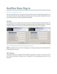
RealFlow 5. Manual Version 1.100Introduction | 11ready to pick up your particles and perfectly suited for particle swapping or foam creation.Former RealWave-specific emitters are now part of the software’s wave creation tool.DaemonsDaemons are now multi-threaded and can affect all standard fluids, dynamics nodes(including MultiBodies) and mist particles. Most daemons can also be used for Hybridoparticles. The new filter daemon let’s you specify certain characteristics and evenexpressions to shift particles to a container emitter.“Caronte” – Rigid Body Dynamics"Caronte", the new rigid body dynamics engine has been completely rewritten for moreperformance, better collision detection and easier handling. Rigid body dynamics nowsupports more than one processor and constraints have been replaced by MultiJointobjects.“Caronte” – Soft Body DynamicsThis tool has also been rewritten from scratch. It’s much faster and more reliable, and alsooffers a completely fresh interface with new parameters. An important change is that softbodies no longer use particles to describe the bodies’ vertices.RealWaveA statistical spectrum modifier used for sharp cresting waves. Also it’s possible to exporttileable displacement maps for large ocean surfaces. You’ll additionally find a Gerstnerwave modifier and the possibility to import file sequences.Curve EditorThe curve editor has been vastly improved and now supports the selection of keys overmultiple curves. New tools have been added for better and easier curve drawing andprocessing. It’s also possible to mix keyed curves with expressions. Sophisticated toolsfor navigating the graph window and for copy/paste actions have also been implemented.Python scriptingThe Python interface provides commands and support for the new functions. Additionally,a completely new structure for event-based scripts has been introduced. It’s now alsopossible to manage scripts in a clearly arranged tree structure and use the new autocompletefunction for the implemented statements. Another improvement concernsRealWave meshes – with RealFlow 5 you can affect vertices along all three axes.MeshingThere are two completely new ways to create meshes. Firstly, you can calculate mesheson the fly from millions of particles, in conjunction with the new grid fluid solver Hybrido.Experienced users will find some similarities to the traditional meshing engine in RealFlow4. The other new meshing approach provides the same tools as Next Limit’s RealFlowRenderKit. The RenderKit meshing engine is also part of Next Limit’s Maxwell Render 2.0software and can read RealFlow’s particle BIN files. This ability to exchange data betweendifferent programs and render engines is fairly unique.New Objects And Object FeaturesRealFlow 5 provides a new Cross object. Users are now also able to load image mapsand image map sequences for some particle-fluid interactions. Parameters, like “Particlefriction” or “Sticky”, can be specified as maps, showing zones with different values basedon the greyscales of the map. MultiBody objects can be used to load a large number ofindividual items within a single node – this also drastically shortens import time.Plug-ins And SDKProgrammers and developers now have the option to write their own extensions andcommercial plug-ins for RealFlow. A complete Software Development Kit for C/C++provides the necessary tools and functions to get you started.GUIRealFlow’s interface is now even more friendly. New icons, a cleaner layout and fast OpenGLshaders for displaying meshes have been added. The simulation events window nowprovides a tree structure for fast access to your event scripts. Another very useful additionis a new internal Movie Player to create animated previews directly within RealFlow.Help SystemA completely new and integrated help system is also part of RealFlow 5. The help systemis directly based on the new manual and provides detailed information for all features,functions and parameters. It also includes the Python scripting reference.© Next Limit Technologies 2010

RealFlow 5. Manual Version 1.100Introduction | 1264-Bit SupportAll versions of RealFlow 5 (Windows, OS X, Linux) now support 64-bit operating systemsand can make use of the entire available memory. At the moment, OS X 10.6 supports thismode only for the Node Version, but we’re working on a GUI version. 64-bit applicationswere designed to make use of the entire amount of RAM installed in your computer, butdo not necessarily accelerate simulation speed.A three dimensional domain gives the user the possibility to look at an object, or an entirescene, from all sides. This is also called perspective view and you can virtually walk aroundthe objects. RealFlow also knows two dimensional views, like front, top or side. There, thepoint of view is fixed and can only be altered within two dimensions. This change of viewis called panning.2.03 Basic ConceptsRealFlow can simulate highly complex interactions between various objects to mimicnatural phenomena, such as fluids, collisions or deformations. Though there’s an enormousamount of physics and maths behind these simulations, the user actually doesn’t have tobe proficient in natural sciences. Everything is done by the software and the includedtools. Nevertheless it’s definitely useful to have a basic understanding of natural processesand some fundamental physics. This understanding will help you to get a feeling formotions, scales and the plausibility of your simulations. Another reason is RealFlow’s modeof operation, because many parameters have a physics background, for example density,mass or friction. Another concept concerns programming. Since each software has itslimits, RealFlow provides interfaces to Python and C++ to overcome these restrictions.a. The Third DimensionRealFlow’s workspace is three dimensional. This means that the position of an object orparticle is always described by three coordinates, named X, Y and Z. This concept is notonly valid for positions, but also for rotation, scale and many other characteristics, like thepivot point. In terms of dimensions, e.g. for a cube, the coordinates are also known aslength, width and height.To specify an object’s coordinates it’s important to have a reference point. This specialpoint is called “origin” and is located at the scene centre of the scene. Following theXYZ notation, a particle with coordinates of [ 0,0,0 ] is directly located in the origin. InRealFlow the XYZ space is displayed as a system of three axis which represent a so-calledcoordinate system. A set of two coordinates (XY, XZ or ZY) is called a plane and is alwaystwo dimensional. It’s also possible to create a coordinate system from just two axis. In thiscase the origin’s coordinates are [ 0,0 ].Visualization of a complex velocity vector field in RealFlow.The 3D space is the place where your simulation happens. It includes a grid to let the userknow where the origin is. Typically, a 3D scene also includes a camera, though this isn’tabsolutely necessary. With cameras it’s easier to store and recall certain views or followother items in the scene. For this purpose, RealFlow supports multiple cameras and youcan even import previously animated (or static) cameras from various applications.Everything that’s created in RealFlow or added to the scene is also part of the 3D spaceand can be manipulated there. Another important feature of 3D programs is shading toimprove the spatial impression. RealFlow offers different shading methods and you canalso decide whether you want to illuminate the objects with one or two light sources.Together with the four standard views you have full control over your 3D elements.© Next Limit Technologies 2010

RealFlow 5. Manual Version 1.100Introduction | 13b. RealFlow NodesIn order to calculate simulations, RealFlow needs objects – so each item that’s inside ascene could be considered as a node. But this kind of definition is not enough, because theobjects have different functions. Some are used to create particles, others add forces orwaves. It makes sense to group the RealFlow objects according to their functionality – forexample emitters, daemons or RealWave surfaces. These groups also include “traditional”objects, like spheres or vases. Traditional objects are different from RealFlow’s otherobject groups, because they consist of polygons and vertices, representing the shapeyou finally see. Emitters or daemons also have a graphical representation, but that’s onlyfor visualizing their location and dimension, because an emitter cannot collide with adaemon, for instance. The emitter node itself isn’t able to interact with a cube either, butthe particles, spilled out from this emitter, can do so.RealFlow’s different node types in the Icon Bar.Real or traditional objects also have the ability to act as simple collision objects for fluids,as rigid bodies with physical characteristics, or as ductile soft bodies. It doesn’t matter ifthey’re native RealFlow objects or imported. No objects have this ability. These are thenode classes you can use: domains, emitters, daemons, polygon objects, meshes, wavemeshes and cameras. All these types and their functionalities are explained later.c, Particle SystemsParticles are generated by emitters and their total amount represents the fluid. Eachparticle can be seen as a point in 3D space with certain properties, like velocity, positionor mass. Though it’s possible to address each particle individually (e.g. with scripting), itcannot be discussed as a single object. However, a particle has a physical dimension andis capable of influencing other objects. The final shape of the fluid is a result the totalamount of particles and forces acting1. between the particles and2. on particles from the outside.Turbulent interactions between different fluid types.d. Grid Fluid DomainsPrevious versions of RealFlow exclusively used a grid-free approach to simulate thebehaviour of fluids. This concept is perfectly suited for smaller scenes, where a certainamount of details is needed, but with large-scale simulations it quickly reaches its limits.To overcome this restriction, RealFlow now can make use of predefined grids, also calleddomains, with customizable resolution. The idea is to create just the “core” of the fluid ata fairly low level of detail, making it possible to rapidly solve the fluid equations. Whenevera higher amount of detail is required, RealFlow can detect these areas and add standardsplash particles to refine the simulation. Splash particles are again generated within certainareas, defined by the user.This sophisticated hybrid technology makes it possible to adjust the quality and level ofdetail exactly to your specific needs at maximum simulation speed! Another advantage© Next Limit Technologies 2010

RealFlow 5. Manual Version 1.100Introduction | 14is RealFlow’s ability to generate secondary particles, for example splashes, from cachedsimulation data – even over a network. With this workflow it’s much easier to createlarge-scale simulations, because you can keep the core fluid particles and develop severalversions with splashes and mist, or write out everything in several passes for betterpipeline integration and post-processing.e. ForcesA force causes an object to change its velocity. This brief definition already containseverything you need to know. Whenever there’s a force acting, then the particle (whichis here considered as a very small object) or object becomes accelerated and changes itsprevious position. There’s only one binding condition: the object must have mass, becausea massless object is not affected by forces. The basic formula for forces is:F = m · aF is the symbol for force, m stands for mass and a defines some kind of acceleration.Acceleration could be gravitational acceleration, for example, also called g. By simplysetting m = 0, you can see that the resulting force F becomes 0, too. That’s why everyobject needs a certain amount of mass to become accelerated.In RealFlow an external force can be introduced by adding one or more daemons to ascene. Very popular forces are gravity, wind, drag and vortex. A big plus is that all theseforces can either act globally on the entire scene, or locally on selected objects, within adefined volume. Forces can affect particles as well as objects. In RealFlow it’s possible toadd as many daemons as you want.f. Dynamics And AnimationThis is another very important concept, because these methods are fundamentallydifferent, though both share a common characteristic: motion. Animation is a manual (orsemi-automatized) process of recording certain properties at particular points in time. Thisis method is also known as keyframing. At each point a new key is set, containing the newvalues. The differences between the current and the previous key are interpolated by thesoftware, resulting in a motion. RealFlow can handle both imported animation keys from3D applications and RealFlow’s tools.On the other hand, dynamics doesn’t need manually set keys. The user simply definesstarting values for various parameters (for example velocity, position, mass etc.) and addsforces. The simulation software then calculates the entire motion of the objects, basedon real physics. With dynamics it’s possible to simulate interactions between differentobjects in a physically correct way. With manually set keys this would be a really trickytask requiring an enormous amount of experience.Of course, the dynamics simulation is recorded, too, to enable playback or export thedata to a 3D software, but actually this isn’t absolutely necessary. With identical startingvalues we could repeat the calculation again and again, and the result would always bethe same – at least theoretically. Another idea is to write an animation key for each changein position and rotation. This method is called baking and can be performed either withPython scripting or inside some 3D applications.A third type of motion recording is expressions. An expression is a formula that tells anobject how to move. With expressions, animation keys aren’t needed and it’s not necessaryto introduce forces. Expressions can also serve as a starting condition and the object’smotion becomes influenced by forces on its way. Expressions are a very convenient wayto create repetitive motions, for example, without the need of Python scripts. Anotheradvantage with expressions is the fact that they are multi-threaded, while Python can onlyuse one processor of a computer.g. ScriptingScripting is a really powerful extensions and once you’ve started with it you’ll never lookback. Of course, it’s not easy for beginners to learn the basics of a new software and ascripting language. Python scripting was introduced in RealFlow version 4, giving the usersa powerful tool to influence RealFlow independently from most of its technical restrictions.Next Limit chose Python, because it’s an easy-to-learn and freely distributable language.Scripting doesn’t only allow the user to influence particles or objects, it makes it possibleto automatize certain repetitive tasks, change various parameters from thousands of itemsin a single pass, write out text files, bake dynamics, create customized simulation datafiles, or turn simulation and dynamics properties on and off, to name but a few. CreatingPython scripts under RealFlow is discussed separately, since it’s a very important andversatile feature. There’s a basic course contained in this manual.© Next Limit Technologies 2010

RealFlow 5. Manual Version 1.100Introduction | 17particle fluids and objects. It’s not necessary to introduce three force daemons and makethem exclusive to the related nodes. By setting different scales for the various solversyou’ll be able to adjust everything to your needs without having to alter all the daemonsindividually each time. Higher force scale values create higher accelerations, lower settingshave the opposite effect.2.04 Notations And AbbreviationsIt’s necessary to introduce a few notations making it easier for you to follow this manual.The abbreviations are actually very common and most likely they’re known from otherapplications, but for the sake of completeness they’re provided here.c. Keys And ShortcutsIt’s often necessary to use certain combinations of keys to activate a function or switch toa particular mode. Sometimes they’re combined with mouse buttons:Rotate viewport: Alt + LMB“Press the Alt key on your keyboard, hold it and drag the mouse while holding the leftmouse button.”Switch to flat shaded mode: 3“Simply press the 3 key on your keyboard. A mouse action is not required here.”a. Commands And MenusA sequence of commands is always separated by an angle bracket “>”, for example:Menu Bar > Edit > Add > Grid fluid > DomainSelected object > Node Params > Fluid > Densityb. AbbreviationsCommon abbreviations are:LMB Left Mouse Button RMB Right Mouse ButtonMMB Middle Mouse Button MMW Middle Mouse WheelOS Operating system GUI Graphical user interfaceRFRK RealFlow RenderKitRBD Rigid body dynamics SBD Soft body dynamics3DS 3D Studio MAX C4D Cinema 4DLW Lightwave XSI Softimage© Next Limit Technologies 2010

RealFlow 5. Manual Version 1.100Introduction | 183 Getting started with RealFlowNow it’s finally time to start RealFlow. Experienced users will surely get along easily,though the interface has been updated. New customers should first read through theentire section about RealFlow’s graphical user interface and its numerous possibilities.After RealFlow has launched, a window appears. This is RealFlow’s Project manager andcontains functions to create a new scene or open an existing file. By default, all new filesare created in a certain directory. This specific path can be changed permanently underPreferences, but for the very first project it’s currently not necessary to alter this path.A scene can be opened with the appropriate button on the upper right or via the “Recentprojects” list. To open a file from this list, simply double-click on the desired project.As long as the Project Management window is visible, it’s not possible to access theunderlying windows or panels. You first have to either close the window or define/opena project. Now enter a name of your choice and click on “CREATE A NEW PROJECT”, ordirectly define a new path to a custom directory and then create the project.If you want to have a look at the project’s directory, choose from the menu bar:File > Open Project Folder...This command opens an external window from the operating system to check whetherall files have been created or not. The actual RealFlow file has the project’s name andthe extension FLW, e.g. “beach_scene.flw”. It’s important to understand the structure andhierarchy of the project’s directory, because RealFlow stores and reads files directly fromthese folders. Some of these directories are only created in case of need:gridThis is the place for all simulations file from the new large scale fluid engine. The “pxy”subfolder contains proxy files.initialStateHere, RealFlow stores all files that can be used to start simulations from previouslyrecorded states, e.g. relaxed and calm fluid volumes.meshesPolygonal meshes from grid and traditional fluid simulations can be found here.RealFlow’s Project Manager under Windows XP ® during startup.First of all you must enter a “Project name”. By clicking on the “CREATE A NEW PROJECT”button, RealFlow generates a set of different folders, where the simulation files wil bestored later. All these folders are grouped under the project’s main directory, carrying thename you’ve entered before. If you didn’t specify an alternative path, everything is storedunder the program’s default location, which is printed one line below. “Full path” displaysthe entire path to your scene including the previously entered project name.particlesAll particle files with the BIN (“binary”) extension. In case of need you’ll also find additionalfolders for mist emitters. These directories carry the name of the appropriate node andonly appear when mist particles were simulated in cache mode.imagesWetmap and foam-map sequences can be found here.logThe log file is stored in this folder. It stores exactly the same information from RealFlow.© Next Limit Technologies 2010

RealFlow 5. Manual Version 1.100Introduction | 19objectsThis folder contains dynamics data and files for geometry/object exchange.wavesRealWave cache files (RWC) can be found here, but RealWave surface deformation files(SD) are located under “objects”.previewRealFlow stores all preview-based image sequences and videos here. The folder containstwo directories, called “images” and “video”. “video” is also the home of a “frames” folder,where all images from automatically generated video previews will be stored.foamThis folder is created automatically on demand and contains foam cache files. Withactivated foam-maps, another directory is created storing the textures. This directorycarries the name of the related grid fluid domain.mistLike foam, this directory is only created on demand. You can find the mist cache files here.These directories are not only important for storing RealFlow files, but also for importingsimulated data into your 3D application. The “objects” folder is of special importance,because it’s recommended to store all exchange files you’ve created within this directory.By default, RealFlow looks for SD files there and you don’t have to browse through yourhard disc.© Next Limit Technologies 2010

RealFlow 5. Manual Version 1.100Introduction | 204 RealFlow’s User InterfaceRealFlow comes with an default layout that’s always applied while starting the application.This standard interface can be changed to your individual needs and then defined as anew start layout. The initial screen is almost the same for all operating systems. Only afew buttons, some system specific font faces and handles are slightly different. The layoutitself is separated into several sections, containing everything you need for setting up aRealFlow scene, modifying objects, and accessing all of the software’s parameters andnodes. To get you off to a good start, it’s a good idea to classify the different parts:Node Elements containViewports, Nodes, Node Params, Exclusive Links, Global Links, Right-click MenusMenu Bar containsMenu BarIcon Bars containFile Bar, Edit Bar, Nodes Bar, Transformation Bar, Scripts BarTimeline Elements containTimeline, Simulation Control, Miscellaneous Tools, Animation Tools, Timeline Control4.01 Window ToolsThe top bar of each panel contains a couple of different symbols and icons, two on the left,three on the right. Windows and Linux users will immediately recognize them:The first two symbols represent functions for changing a window’s content and differentsplit views. The following three icons represent functions for A) minimizing, B) maximizingand C) closing a window. In this context, “Maximizing” means in that the window isdetached from the layout and available as a floating window.RealFlow’s panels don’t have a fixed assignment. Each window can easily be transformedinto another one. For example, it’s possible to convert a viewport window into a CurveEditor, or a Global Links panel into a Node Params window. By clicking on the symbol onthe far left, RealFlow opens a little menu, showing all of its available types. Active windowsare displayed in grey, invisible ones are white.The second icon on the left is used to create various arrangements of split windows. Youcan choose between “Split Vertical”, “Split Horizontal” and “Split Quad”. Of course, thisoption only makes sense with RealFlow’s viewport. Applying “Split Quad”, for example, tothe Nodes panel creates three additional viewports. You can apply as many windows asyour operating system can handle. The panels are also resizeable and for this purpose theinterface provides a slider. Simply position your mouse cursor between two windows toactivate the drag mode – now it’s possible to shift the borders.Other Windows containMessages, Curve Editor, Simulation Events, Batch Scripts, Movie Player, Help Viewer, JobManager4.02 ViewportsThese are surely the most striking windows and contain all scene elements. You caneasily toggle between 2D and 3D views, choose from different shading modes and displayvarious information about the nodes, e.g. the amount of grid cells. The viewports are fully© Next Limit Technologies 2010

RealFlow 5. Manual Version 1.100Introduction | 24or disappear automatically according to the activated options, e.g. for rigid or soft bodydynamics.uuThe individual settings, panels and parameters for all Node Params panels areexplained in detail in combination with the appropriate objects and their attributes.To change a certain value it’s necessary to left-click on it to make it editable. Once it’shighlighted, you can enter the desired value. Please note that some parameters havecertain ranges, for example between 0 and 1, while others accept almost any value, evennegative settings. Invalid settings won’t be accepted and will automatically reset to thepreviously given value.Most of the parameters under Node Params can be animated. For this purpose it’s possibleto set keys or open the Curve Editor which also provides several methods for animation(a detailed explanation of the Curve Editor’s functions can be found on page 242). To setor delete keys and curves, simply right-click on the desired value to open a little menu,showing various entries. Values that cannot be animated won’t show in this menu. Pleasedon’t activate/highlight the values meant to be changed! In this case you’ll see anothermenu with entries for undo/redo and clipboard functions.The result is an explanation of the current property. Together with the new Help Vieweryou have a powerful, though easy-to-use, help system that’s seamlessly integrated intoRealFlow.4.05 Global Links And Exclusive LinksThese panels can only be explained together and they also have a very close relationshipto the Nodes panel. By default, you’ll see each new object inside the Nodes panel aswell as under Global Links. As long as the “Add to Global links” option is active, RealFlowassumes that all items are able to interact with each other. The idea behind exclusivelinks it that you have the possibility to make certain invisible to other objects. To achieveexclusive links, it’s important to know that you have to maintain a certain hierarchy. Thismeans that you cannot arrange the links randomly, otherwise you’d cut interactions:• Objects and emitters have to be placed under RealWave nodes• Daemons must be organized under objects and emitters, including grid fluid emitters• Objects must be placed under emitters• Objects must be grouped under other objectsA Node Params sample menu for a square emitter.Node Params additionally provides an internal help system that can be activated with aright mouse click or the F1 key. The right mouse help is only shown by clicking on one ofthe main riders.The F1 help system shows information about the various parameters. Some of theseexplanations might appear very familiar to you and that’s no coincidence. To give youthe best available information, RealFlow’s help system is entirely based on this manual.To activate it, simply click on the desired parameter to highlight it and then press F1.Examples for Exclusive Links with correct hierarchy.© Next Limit Technologies 2010

RealFlow 5. Manual Version 1.100Introduction | 26a. The File MenuThe “File” menu helps you to organize your projects and call existing simulations, but it’snot responsible for setting up export settings to store simulation results. Please note thatthis feature is located under “Export”. These are the entries and shortcuts of the “File”menu:Update SD SceneWith one click you can update a currently loaded scene file, especially after makingchanges inside the 3D software and writing out a new SD export file.Summary Info...The function displays information about the total number of nodes and their properties,such as number of polygons, vertices or particles, together with physical parameters ofemitters. Additionally you can add a description of your scene that will be stored with theproject.Recent workspacesTo get a list with recently opened project files, choose this entry. You can directly accessthese files without having to open RealFlow’s Project Manager again.Preferences...This command opens a new dialogue window containing parameters for adjusting generalcharacteristics of RealFlow: Layout, controls and environment parameters, for example.Under OS X this function can be found under the “RealFlow” entry.New ProjectYou can close the current project and open the Project Management window.Open Project...Choose this option for opening an existing project.Save ProjectSave the current project with menu entry.Save as...To save the current project with a new name this action is required.RevertOpens the last saved version of the project.Open Project Folder...Opens the folder containing the project.uuSince the Preferences section contains many important settings for customizingRealFlow, it’s discussed under an own chapter starting on page 45. There you’ll finddetailed information about the meaning and influence of the various parameters.ExitClose RealFlow here. Before the program quits you’ll be asked to save all unsaved changes.In OS X this function can be found under the “RealFlow” entry.b. The Edit MenuThis menu provides functions for your work with RealFlow nodes.AddAdd opens several submenus containing all kinds of RealFlow nodes. For faster access, thenodes are grouped and can be added directly to scene.RemoveRemove the selected node(s) from the scene.© Next Limit Technologies 2010

RealFlow 5. Manual Version 1.100Introduction | 27CopyWith this tool you can easily copy and transfer different transformation data fromone node to another. You need two nodes for this operation – the order of selectiondetermines, which item will be the source object. You can either copy and transfer dataindividually for “Position”, “Rotation”, “Scale” or “Shear”, or perform all changes togetherwith “Transformations”. The selection doesn’t require nodes of the same type!SnapAgain, this function depends on the order of selection and requires two nodes. The firstobject is used as reference. “Nearest side” will bring the two nodes as close as possibletogether. The “Nearest side (expanding)” tool stretches the target object until it touchesthe reference node.UndoThis action can be repeated to go back several steps, but can also allocate a lot of memory,especially when you undo/redo emitter-based actions with large particle amounts. If the“Undo” option needs too much memory, you should consider freeing it up with the “ClearUndo Stack” function from the Tools menu.RedoRedo the previous action.MoveSwitches to Move mode. When this mode is active, the selected node shows a cross witharrowheads.RotateSwitches to Rotation mode. In Rotation mode, the active node shows surrounding circleshapedhandles for adjusting the desired transformation quickly by dragging the mouse.ScaleSwitches to scale mode and adds cubic handles to the node. By dragging them you caneasily adjust an object’s size with the mouse.Add KeyframeThis submenu consists of four entries. Instead of selecting and keying the appropriateparameter under Node Params > Node, you can also use “Position Key”. It automaticallywrites keys for the item’s X, Y and Z values. “Rotation Key” works exactly like “PositionKey”, but is responsible for recording rotation value. The workflow with “Scale Key” is thesame as with “Position Key”. If you want to write animation keys for position, rotation andscale, then you don’t have to do this for each attribute. Choose “Transformation Key” toadd keys for all parameters.Freeze TransformationsLocks all transformation to the current state.Reset TransformationsResets all transformations to the object’s starting values.Clone SelectedA clone object is a copy of the current object which gets its default values from theoriginal. This function exclusively works with standard emitters, daemons and objects.Imported objects from SD files cannot be cloned, too.Back culled selectionIn several cases it’s required to select polygons from an objects, for example for emittingparticles. Normally, RealFlow doesn’t differentiate whether the polygons are visible to useror not. With this option enabled, you can only select polygons which are really visible toyou and hidden faces won’t be considered.© Next Limit Technologies 2010

RealFlow 5. Manual Version 1.100Introduction | 28c. The View Menu“View” provides functions for customizing the viewport windows and various shadingmodes. It is surely one of the most often used menus during creating and simulating yourscene. Please keep in mind that “View” does not manage the visibility of a node. If youwant to make an object invisible or visible, you need the according Display panel. Theentries of “View” can be seen here:SceneYou can display the entire scene as “Bounding”, “Wireframe”, “Flat Shaded” and “SmoothShaded”. The specifications for these modes are the same as for “Element”. Additionally,there are “Wireframe back faces” to show the inside of objects when their normals areinverted. “Textured” draws an object’s texture based on its UV coordinates.Point of ViewYou can change the current viewport view to “Top View”, “Front view”, “Side View”,“Perspective View” and “SceneCamera View”. The last view option is only available withat least one camera.Reset ViewRedraw the viewport to switch back to RealFlow’s default point of view.Fast ViewDisplays objects as bounding boxes when moving, rotating or scaling. Especially with largescenes and many objects, this is a good means to increase display speed. Even standardfluid particles are drawn as boxes, while grid fluids and daemons are still represented asparticles.View GridTurns the grid in the viewport(s) on or off. “On” is the default setting.ElementThis submenu is used to display the currently selected object in one of the following modes:“Bounding Box” is a wireframe box, covering the volume of the object. There are no visibleshapes or poylgons, even emitters are displayed as simple boxes. In “Wireframe” mode,only the polygon edges are shown and you can still see underlying objects. With “FlatShaded” the object shows its faces as shaded polygons. The faces of “Smooth Shaded”objects appear even. Higher polygon numbers create better and more accurate results.View Preview Safe FrameTo make use of this option, a camera is required. After the camera view has been enabledyou can see two frames around the viewport. The outer frame is in cyan and exactlymatches the camera view, independent of the viewport’s aspect ratio. The inner frame isblue and shows the title-safe area of the current view.View Preview CaptionWith this option it’s possible to print some basic information about the current scenedirectly to the viewport. The data are written to in the top right-hand corner and representyour settings underPreferences > Display > Top Right CaptionThere you can enter either your own text or choose from a couple of variables, for exampleframe rate, frame width or the scene’s name.© Next Limit Technologies 2010

RealFlow 5. Manual Version 1.100Introduction | 29Follow SelectedDuring animation the currently selected node will always be in the viewport’s centre.d. The Layout MenuThis section provides access to all RealFlow windows and has the following entries:The image above shows a viewport without a grid, but with “View Preview Safe Frame”and “View Preview Caption” enabled (the labels are enlarged for better visibility). Thepreview caption was defined under the previously mentioned Preferences section, usingthe following text/variables:Grid Fluid Comparisons @ $(FPS) frames : $(FRAMEWIDTH) x $(FRAMEHEIGHT)View Screen TextureYou can fit a bitmap into a viewport as a background. If you have several viewports open,it’s possible to turn the loaded picture on or off for each viewport separately. RealFlowdoesn’t store the loaded image and it has to be applied with each launch.Load Screen Texture...Choose a bitmap to load into the viewport as a background. Supported file formats areTGA, BMP, JPG, PNG and TIFF.Center SelectedCentre the select object(s) in the current viewport.Save LayoutWith RealFlow you can create your own layouts and interface arrangements and savethem to a default folder, specified under Preferences.Load LayoutTo load a layout from any folder, choose this entry. This is normally used, when there areno entries listed under “Apply Layout”.Apply LayoutHere you can find a list with all available layouts under RealFlow’s default folder. “Default”resets everything to the initial layout. This configuration is also specfied under Preferences.© Next Limit Technologies 2010

RealFlow 5. Manual Version 1.100Introduction | 30Clean LayoutCleaning a layout means that all menus and panels will be removed and the viewportsexpanded, filling almost the entire screen. The only remaining elements are IconBars, Timeline and Timeline Control. To switch back, go to “Apply Layout” and select aconfiguration.Clear MessagesIf you want to get rid of previous notifications in the Messages window, you can call thisfunctions. The window becomes cleared, but the associated log.txt files is concerned inthe action. You still have the complete message history stored there, unless you quit andrestart RealFlow.Single ViewLaunches an independent panel containing a single viewport.Quad ViewLaunches an independent panel with four equal viewports.NodesLaunches an independent Node panel.Exclusive LinksLaunches an independent Exclusive Links panel.Global LinksLaunches an independent Global Links panel.Simulation EventsLaunches an independent Simulation Events panel.Movie PlayerLaunches the internal Movie player.Job ManagerLaunches an independent Job Manager panel for network simulations.Help ViewerLaunches an independent Help Viewer panel for RealFlow’s built-in help system.“Independent” means that RealFlow opens a floating window that’s not integrated intoyour current user interface. If you open an already displayed window, it will be detachedfrom the user interface and shown separately as a floating window. The empty space willbe replaced with another window.uuThe feature set of the windows listed above are explained individually, becausemany of them offer a wide spectrum of different functions and options.e. The Tools MenuTools provides several useful functions for managing memory and RealFlow issues. Manyfunctions open new windows with extensive function sets, helping you to accelerateworkflow or free computer resources.Node ParamsLaunches an independent Node Params panel.Curve EditorLaunches an independent Curve Editor panel.MessagesLaunches an independent Message panel.Batch ScriptLaunches an independent Batch Script panel.© Next Limit Technologies 2010

RealFlow 5. Manual Version 1.100Introduction | 34RealFlow particle bin file (single)You can also load any available BIN to the current scene.Nodes from XMLThe XML format is a versatile and flexible file format. RealFlow now supports the ExtendedMarkup Language format for easy data exchange. Nodes, previously saved with “Selectednodes as XML”, can be loaded again with this function. XML files can be edited and changedwith any ASCII-capable text editor! In some situations it’s also helpful to export nodes oreven entire scenes for backup purposes.h. The Commands MenuThis menu can be used to organize custom and system script files. It contains somecomplex functions with versatile features.is also valid for C++ programs, but there there the programming requirements arehigher.Please bear in mind that Next Limit cannot support 3rd party scripts.User CommandsLets you define certain scripts to act like an integrated function of RealFlow. By defaultthe submenu is empty.System CommandsThis shows the included system scripts so that you can call them like integrated functions.Update MenuIf new scripts are not displayed, we recommend that you use this command.The Add Script WindowRealFlow provides the possibility to integrate your custom scripts to the user interface.Once they’re loaded and added to the Scripts Bar they can be used like an internal function,similar to the system scripts (see page 38).AddThis function provides three options for updating and editing the Scripts Bar. All functionsopen the Add Script window, which is described a little later on the right. The “Add”submenu contains three entries: “Script” opens the Add Script manager for adding andorganizing embedded Python scripts. “Script From File” works similar, but launches theAdd Script manager for arranging imported Python scripts. The last action, “Plugin”, callsagain the Add Script manager for organizing scripts from plug-ins.Organize...Opens a window to manage all script types, including DLL-based scripts. The scripts willthen appear under User Commands once they’ve been added. You can read more aboutthis workflow on page 35, “The Organize... Window”.uuUser scripts normally require at least some basic knowledge of Python scriptingto make them run. The complexity of the freely available user scripts varies greatlyand there’s no guarantee that they will really work for your special demands. This© Next Limit Technologies 2010

RealFlow 5. Manual Version 1.100Introduction | 35If you want to make use of already existing scripts, it’s a good idea to visit RealFlow’spopular scripting page. It contains dozens of programs, created by other users andRealFlow developers. These scripts are free to use and can be integrated into RealFlow.Many of them even contain icons. By the way, it doesn’t matter whether you want to addself-written or downloaded user scripts to the interface. Now lets have a close look at theAdd Script window:1. The script tree with three columns “Name”, “Shortcut”, “Script”2. The button barThe “Name input” field lets you specify a custom name for the script you want to add.This can be any name, but you should avoid double naming! “Edit Script” opens the scripteditor where you can also load and save already pre-stored scripts. From the “ToolBar”menu you can choose the desired toolbar where the currently edited script will be addedto. “Icon...” allows you to choose a custom symbol from your hard disk and the currentlyused icon is shown next to the “Icon” button. Please note that the best format for iconsis PNG. The “Shortcut” menu provides a list of available shortcuts that can be used forcalling your script. Simply select one of the suggestions to attach it to the current script.The script tree contains already existing and loaded user programs to give you an overview.It also shows the current organization of your scripts, including all folders (= groups), thescript’s name, the shortcut and its complete path. Here, it’s not possible to edit or organizethe scripts – the tree is for information purposes only.“New Folder” gives you the opportunity to create a new folder to group the scripts and,of course, it’s possible to rename it. If you want to add a script to a folder, choose yoursettings first and single-click on the desired folder to highlight it. When you confirm with“OK”, the window will be closed and the script will be added to the selected group. Thescript now appears within the Scripts Bar, showing the chosen icon. “Cancel” closes thewindow without applying or saving your settings.uuYou can also specify user scripts as system scripts. For this purpose the sourcecode needs a so-called header, telling RealFlow that the program has to be attachedto the appropriate section of the Scripts Bar. If you’re interested in how to performsuch an action, just open one of the included system scripts.The Organize... WindowRealFlow’s (user script) organizer only works if there’s at least one existing user script,otherwise there’s simply nothing to organize. The window contains two sections:The empty Organize Commands window.The script tree canvas should also look familiar to you, because it has exactly the samelayout as seen under “Add script”. The difference is that it’s fully editable now. To performthese changes the button bar is used:“New Folder” adds a new folder to the script tree – you can enter a new unique namefor it. “Remove Folder” deletes the selected (=highlighted) folder, but please be careful:By removing a folder you’ll also delete the programs grouped under this folder from thescripts tree and the Scripts Bar. “Rename Folder” lets you enter a new name for theselected folder.“Change Properties” is used to alter properties, like shortcuts or the desired toolbar foryour scripts. “Edit Script” opens a new dialogue, similar to Add script, but without thescripts tree. With this menu it’s not possible to edit the source code, but you can specifya new name, a different path, apply a new icon or replace a script. To apply a completelynew script, use the “Add Script” feature. “Remove” deletes a script without removing thehigher-ranking folder. “Close” applies your settings and changes.© Next Limit Technologies 2010

RealFlow 5. Manual Version 1.100Introduction | 36i. The Playback MenuThis menu contains functions for creating video previews and controlling the Timeline.For many playback options there are shortcuts available that can be found next to theappropriate command. The shortcut legend is also different for Windows and OS X.Loop PlaybackPerforms an endless loop while playing back the simulations.Beginning FrameJumps to the first defined playback frame.Previous KeyframeMoves the timeline slider to the previous keyframe.Previous FrameJumps one frame back.Next FrameJumps one frame ahead.Next KeyframeMoves the timeline slider to the next keyframe.Video PreviewYou can automatically create a video from the active viewport with this function. Whenthe images are completely recorded, RealFlow directly assembles a video and opens it inthe Movie Player. Compression settings and preview size can be made under Preferences.Open Last PreviewIf you have created more previews, you can simply call up the last one without searching.Ending FrameJumps to the last defined playback frame.j. The Help MenuHere you can query information about licenses and call internal help functions.Open Preview PreferencesThis option directly branches to the appropriate section of RealFlow’s Preferences.uuThe following commands only affect Timeline properties not the video preview!Play/StopStarts or stops the playback of the recorded simulation.Play/Stop BackwardsStarts or stops the reverse playback.Contents...You can access RealFlow’s internal Help Viewer with this command. The Help Viewer andits versatile possibilities are explained in a separate chapter on page 44. RealFlow’s helpsystem also provides a complete Python scripting reference.© Next Limit Technologies 2010

RealFlow 5. Manual Version 1.100Introduction | 37Key Shortcuts...Use this function to get an overview about RealFlow’s keyboard combinations, embeddedin RealFlow’s help system.Web...Prompts RealFlow to open your default internet browser and launch the RealFlow website.License agreement...Here you’ll find the terms of use and copyright notes. Please read the Software EnduserLicense Agreement carefully, because it contains relevant information about runningRealFlow.Python license...The license for the embedded Python distribution can be found here.Release notes...This is very useful source of information, where you can find all known bugs, for example.If you observe an error, you can first have a look at this panel to check, whether themalfunction is already known or not. If you think the malfunction is really a bug, you cancontact Next Limit’s help desk. Additionally, system and hardware requirements are listedhere, along with the latest modifictions of the software.About...The splash screen shows information about your license.this purpose right click into an empty area of the icon bar to open the display filters. Youcan then enable and disable the desired symbol groups.a. The File BarThe File Bar is a set of three icons for basic file operations.For these functions RealFlow provides shortcuts, too:Create a new project Ctrl + N (Win/Linux) and Cmd + N (OS X)Open an existing project Ctrl + O (Win/Linux) and Cmd + O (OS X)Save the current project Ctrl + S (Wind/Linux) and Cmd + S (OS X)b. The Edit BarThis bar contains a total of five icons. With these tools it’s possible to select one ormore nodes and change their position in 3D space. These tools work exactly like theircounterparts in 3D applications. By holding and dragging the mouse, position, rotation, orscale changes are executed. The fifth icon lets you choose between the global and localaxis system.4.08 Icon BarsDirectly below the Menu Bar you can see a series of different icons and symbols. Thesegraphical buttons provide fast access to the most common and often used functions andobjects. For better accessibility they’re subdivided into several groups according to theirfunctionality.RealFlow even gives you the possibility to create your own icons for custom scripts andadd them to the Icon Bar. The program provides a total of 10 fully customizable segments,called “UsrToolbar 0 – 9”. The following chapters tell you how to create and organize yourown toolbars. Another feature is that you’re able to filter the contents of the Icon Bar. ForThe four basic transformations are also available via shortcuts:Select nodeMove toolRotate toolScale toolpress Shift or Ctrl/Cmd for multi-selectionWERThe first four tools can be used to select nodes from the active viewport or the Nodespanel. The viewports provide another option: Simply draw a virtual rectangle around© Next Limit Technologies 2010

RealFlow 5. Manual Version 1.100Introduction | 38one or more objects to select them at once. The “Select node” tool supports hierarchicalselection – ff a node can’t be selected directly from the viewport, because it’s overlappedby other objects, click onto the desired node until it becomes active. Of course, you canselect it from the Nodes panel, too.c. The Nodes BarEach icon represents one of RealFlow’s object groups. The order is: grid elements, particleemitters, daemons, objects, meshes, cameras, RealWaves and IDOC elements.e. The Transformation BarThis toolbar is new in RealFlow 5 and provides tools to transfer position, scale, shear androtation data easily from one object to another. You simply have to select two nodes fromthe Nodes panel and/or the viewport and click on one of these buttons. The transformationdata will be copied from the first selected object to the second one. As you can see, theorder of selection plays an important role. The functions are not limited to objects of aparticular type – properties can also be transferred from objects to emitters, for example.Clicking on an icon will open a list of all available elements. Choosing the desired objectfrom one of the lists, also places the item in your scene. You can repeat this process asoften as needed.d. The Scripts BarThis icon bar contains the so-called system scripts. These are ready-to-use scripts thatdon’t need further adjustments or programming. You can open and organize these scriptswith the Commands Menu, too (see page 34). The system scripts can be used like anyother of RealFlow’s commands and they even have shortcuts.Currently the following system scripts are available: Change resolution, Compute vorticity,Normalize Age, Maya Cache Particle Loader and Build Meshes.By clicking on an icon the chosen script starts working. Please note that some scripts havecertain requirements, e.g. the existence of a mesh node or a particle emitter. Some ofthese scripts might also appear rather slow, due to the fact that Python-based calculationsare always single-threaded. This limitation is not RealFlow-specific, it’s caused by thePython programming language, which supports only one CPU or core.TransformationsTransfers all available node data to the target object.PositionCopy only the position data with this button.ScaleOnly the node’s scale information will be transferred.ShearClick on this button if you want to copy shear properties.RotationThe current rotation angles are shared.The second part of the transformation bar concerns snapping. These functions calculatethe nearest sides between two selected nodes and snaps them together. The first selectedobject is the reference and won’t be repositioned when the second node is translated. Thismode is especially useful for object dynamics – for example brick walls.Nearest sideBrings two nodes together as close as possible.Nearest side (expanded)Stretches the target node until it touches the reference object.© Next Limit Technologies 2010

RealFlow 5. Manual Version 1.100Introduction | 394.09 TimelineRealFlow’s Timeline isn’t just a simple time indicator – it’s a versatile tool that gives youlots of information about a simulation. The timeline slider can be moved back and forthand will let you preview the simulation, but only if the simulation data was cached to disk.In this case, calculated frames are shown in orange.By default you can also see a range between 0 and 200. This is RealFlow’s standardsimulation and playback range, depending on the appropriate preferences. Start and endframes for playback can be changed any time with the fields to the left and to the rightof the timeline bar. The second field on the right is used to specify the simulation rangeIf you’ve imported an SD file for geometry or animation data exchange, there’s alwaysan animation range saved with the file, regardless of whether there are any animatedelements in your file or not. This range can be defined by the user in the plug-in’s exportsettings. In this case, an additional line appears, indicating how many frames wereimported/exported with the SD file. Please note that the yellow line doesn’t have anyinfluence on the simulation length! It’s just a visual control of how many frames have beenstored with your imported scene.be to fill the glass. By locking the simulation you can do this for an exactly defined rangeof frames (= “Frame countdown”). After the glass is filled with particles, you unlock thesimulation and the animation can proceed. You don’t have to specify a certain range forthe countdown, because it’s also possible to unlock the simulation manually by clickingon the lock button whenever you want it. With this easy method you can save time,because you don’t have to split the simulation into two or more parts – filling the glass andperforming the animation. All this can be done within a single file. In other words, lockingthe timeline prevents RealFlow from exporting any files. This is useful for simulating initialstates. After you get the desired result, set the initial state for the emitter and reset thescene, unlock the timeline and simulate as usual. Now it will start from the initial state.Another very convenient button is “Go to last cached frame”. This directly sets the timelineslider to the last stored frame and so you can directly go on with the simulation.4.10 Timeline ControlThis set of buttons is surely familiar to everyone, as it works exactly like the control fieldin DVD players or video editing programs. Nevertheless it’s worth to briefly explain thefunctions:Another feature of Timeline is the “Lock button” on the left. Beneath this button you canalso find a little triangle. By clicking on it, a mini menu is opened, showing some optionsfor locking a simulation:Locking a simulation means freezing all previously animated transformation or movements.Imagine a filled glass is being poured out – the pouring is animated. The first step would1. Go to start frame2. Go to previous frame3. Play/stop button for reverse playback4. Frame counter / “Jump to frame” input field© Next Limit Technologies 2010

RealFlow 5. Manual Version 1.100Introduction | 405. Play/stop button for normal playback6. Go to next frame7. Go to end frame8. Loop playback sequencefilm formats. Please note that there’s a connection between “FPS Output” and “Time Step”– “Time Step” can easily be used for re-timing or slow-motion effects.The Play/stop function can be triggered by pressing the space bar, too. You can also jumpto the start of the simulation with the left arrow and to the end with the right arrow. Withthe up and down arrows you can count back and forth frame-wise.4.11 Simulation ControlThe Simulation button triggers a simulation. During this process RealFlow performs all ofthe necessary calculations, generates the data files and writes them to disk. The simulationitself obeys several settings that can either be defined globally with Preferences (see page46 and 47) or individually for each scene. For adjusting the settings per scene, simply clickon the little triangle to expand a new menu.RealFlow’s Simulation options allow you to adjust simulation settings for each project.There are three entries: “Fluid Dynamics” and “Object Dynamics” switch the appropriatesimulation engines off or on. By default, they’re activated. The “Options...” part is probablyof higher interest, because there you’ll find all simulation-related settings.The parameters you can see under “Options...” are the standard values from RealFlow’spreferences. They can be overwritten to increase or decrease the defaults for theindividual needs of your current project. It’s recommended to determine the settingsunder preferences globally and then alter them with “Simulation options”.“FPS Output” can be used to either adjust the frame rate to your local TV system or acertain cinematic frame rate. RealFlow’s standard “FPS Output” is 25 frames per secondfor PAL. You can enter any desired value, for example 30 for NTSC or 24 for HD, or otherPlease have look at this example:You enter an “FPS Output” value of 75 and simulate the scene. Once it’s ready you importthe simulation data into your 3D application, you set the internal playback rate to 25 andrender out everything. The result is a movie that’s played back at just one third of theoriginal speed from RealFlow. In other words, you’ve stretched time by a factor of three.“Threads” is also connected to RealFlow’s preferences and adjusted automatically.However, for simulations with lower particles counts, it’s often better to reduce this value.The reason is that distributing simulation data to different CPUs or cores takes a certainamount of time and this process can take longer than the actual calculation step. “Usemax. threads” always simulates with the maximum number of processors.The “Integration” section can be described as RealFlow accuracy. The more time steps, the© Next Limit Technologies 2010

RealFlow 5. Manual Version 1.100Introduction | 41better and more precisely the simulation will turn out. You can choose between “Adaptive”and “Fixed”. The adaptive method automatically calculates the best number of steps withinthe specified range between “MIN and MAX substeps”. “FIXED substeps” can be veryaccurate, but greatly increases simulation time. Interactions between particles and objectsespecially profit from higher substeps, because they improve collision detection.these modes are fast and perfectly suited for previews. The second button is “Reset” andby clicking on it, the entire scene is reset to the initial settings and positions. Withouthaving specified a start frame (input field on the left of the time line), the simulation willbegin from 0 again, otherwise the first frame is the manually defined start frame. If youhave entered a frame, e.g. 30, then the first 30 frames will appear in orange, thoughnothing has been simulated so far.Next to the “Reset” button, you’ll again find an expansion menu with “Reset To InitialState”. By activating this option it’s possible to read from a previously simulated and savedinitial state (which can be compared with a preset), and start the simulation using theseparticular settings.With low substep settings (right), collision detection might fail.A value of 75 substeps is a good average and suitable for many scenes. For testingpurposes, values between 10 and 25 are often enough, while final simulations are mostlycalculated around 100 “MAX substeps”. If you need more precision, it’s sometimes betterto raise “MIN substeps” than to alter the maximum number.It’s often necessary to work with higher “FPS Output”, as in the example above. In thesecases you’ll most probably receive an error message, telling you that you that your “Choiceof MAX substeps is too large”. The reason is that it’s not possible to subdivide a scenearbitrarily and there’s a limit. Fortunately, the error message directly tells you the maximumsubstep you can use for the current settings.The last entry concerns rigid and soft body dynamics. From the “Quality” menu you canadjust the solver’s accuracy within three levels: “Low”, “Medium” and “High”. With “Low“and “Medium” you might observe interpenetration problems or inaccurate collisions, butAn example:RealFlow fluids always carry a certain amount of energy, making the particles bounce andjitter. This motion can be removed by allowing the particles to settle down. Once the fluidis calm, you can define a certain frame as an initial state and resume from this positionwithout creating an extra scene. You can read more about initial states on page 69.The third element of the simulation controls is the progress bar. During a simulation ora meshing task, RealFlow displays the progress for the current frame in percent, so therange goes from 0 to 100.4.12 Miscellaneous ToolsThese buttons are new in RealFlow 5 and contain a set of often-used functions. Theannotations below explain these buttons from the left to the right:© Next Limit Technologies 2010

RealFlow 5. Manual Version 1.100Introduction | 434.15 Simulation EventsSimulation Events substitutes the Events Script window from RealFlow 4 and providesa much more comfortable and well-structured tree view. By expanding the individualbranches, you have access to the pre-built simulation events and you’re able to add yourown scripts there. Since Simulation Events is a regular part of RealFlow’s GUI, it providesthe same control elements as any other window. It can also be integrated into a customlayout.uuScripting is also a fundamental part of RealFlow and you can learn more aboutusing Python in RealFlow’s scripting guide, starting on page 268.The window itself consists of two parts. The first part contains the tree view, andpossibilities to add and edit events-based scripts. To access these functions, simply rightclick on the desired predefined functions, for example “Simulation Pre”. The second partcontains a so-called “Master” tab and it’s mainly there for compatibility purposes whenyou want to make use of RealFlow 4 scenes containing scripts. This window still shows the“old” notation with built-in function for various simulation steps. Another tab is empty, bydefault. If you you choose a script from the tree in the upper section, its source code willbe shown here and, of course, you can edit it.Batch Script can be integrated into a customized layout. Additionally you have a menu barwith several entries. Please also go the scripting section for detailed information abouttheir functionality.4.17 Movie PlayerThis is a completely new element in RealFlow 5, and can be used for playing back previewsequences – not complete videos, although it’s possible to export a video out of theapplication. The Movie Player itself works like any other player and show similar elements.To attach it to the layout, just grab the the windows headline area (“Movie Player”) anddrag it to the desired place and save the layout.4.16 Batch ScriptBatch scripting is a very convenient method to automatize repetitive tasks, such ascreating object arrays, randomizing various parameters or starting multiple project files forovernight simulation. There are many possible fields of application for this kind of scriptingand it’s even possible to start scripts with command line simulations. By default it’s nothingmore than an empty window.The Batch Script panel works like a text editor and has some basic features like tabbing,syntax highlighting and keyword completion. Of course you can copy/paste scripts fromother sources to the Batch Script window.u u You can learn more about batch scripting in RealFlow’s scripting guide, startingon page 271.© Next Limit Technologies 2010

RealFlow 5. Manual Version 1.100Introduction | 44The main part is the canvas, which is empty by default and shows the label “No sequenceloaded”. Directly below there’s the timeline, showing the number of available frames. Youcan easily scrub though the frames by dragging the slider. If you want to restrict playbackto a custom range, then you can enter a start and stop frame in the fields next to thetimeline. The “L” button turns on the loop function.• The Help Viewer. This is an extra window and can be seen as a kind of catalogue.You can navigate through all of RealFlow’s functions by navigating through a clearlyarranged tree menu, use the index function or perform a quick search through theavailable documents.Checking the “Fit” button adjusts the video to the canvas. In this case the currently loadedvideo appears downscaled or cropped. By default the video is displayed 1:1 and thereforethe borders might not be visible. You can resize the player by dragging its edges.“Skip” is used to guarantee a smooth playback. By activating “Skip”, some frames mightbe dropped to guarantee playback at the adjusted frame rate.With the folder symbol you can choose a previously recorded file sequence and load it tothe player. Once the images are buffered, playback starts automatically. The next symbolprovides a function to export the sequence as a video. You can also set this option as adefault under Preferences (see page 51). When you want to store a video, you’ll be askedto choose a video format. Please note that the selection of video formats strongly dependson your operating system and the installed codecs.The following buttons work exactly like their counterparts in the timeline control section.You can start playback or jump to the beginning/end of the sequence and go through theclip frame by frame. The last button clears the canvas. Finally, you can specify the framerate for playback. This field is connected to RealFlow’s Simulation options (see page 40)4.18 Help ViewerUnlike in previous versions of RealFlow, the help system is now an integrated part of theuser interface. Since adequate explanations of functions and parameters are essential,RealFlow’s internal help has been vastly improved and extended. The entire help systemis based on the manual and can be subdivided into two parts:• The F1 help. By selecting a certain parameter under Node Params and pressing F1,you’ll get the appropriate help text for this particular function. RealFlow’s F1 helpis directly connected to the Help Viewer: Below an explanation you can find a link,named “Search in help...”. This function automatically performs a search through allhelp documents and prints out the appropriate results.The Help Viewer’s menu tree includes information about all available nodes. You canexpand and collapse branches of this tree and by clicking on one of the topics, the helpcontents will be displayed. A very user-friendly feature allows you to stack documents withthe help of tabs. You can open, close and manage these tabs as required, to provide fastaccess to frequently-used pages or explanations. To add a new tab, simply right click onthe desired keyword and choose “Open Link on New Tab...”.Under “Index” you can find a complete alphabetical list of RealFlow’s parameters. Thisfeature is useful when you’re looking for a certain parameter, but currently don’t knowwhere it’s located. Instead of the “Index” you can, of course, use the search function.RealFlow’s help search is not a simple keyword look-up. It’s a sophisticated dynamic searchfunction with many options for finding words, expressions similar to your query, and evenBoolean functions, e.g. with or without a certain word. These functions are located under“Advanced search.”© Next Limit Technologies 2010

RealFlow 5. Manual Version 1.100Introduction | 455 Adjusting RealFlow PreferencesThe Preferences window is a comprehensive tool for adjusting RealFlow to your specialneeds. These adjustments not only influence RealFlow’s look and feel, they also have avery strong influence on simulation speed. You can control almost anything and tailor it toyour personal taste or maximum performance. The window is classified into several panelsaccording to their particular function. Though some of these setting have a global impact,they can also be changed individually for each scene, for example “FPS output” or “MAXsubsteps”. To open the Preferences window, please chooseEdit > Preferences... (Windows/Linux) or RealFlow > Preferences... (OS X)The window consists of two parts. The left part is a menu tree with all available sectionsand you can open each one, by simply clicking on it. The appropriate contents are thenshown in the right section.5.01 General“Scenes Folder” contains the path to RealFlow’s default directory where all scenes arestored. Whenever you create a project, RealFlow links to this directory. With “…” youcan easily define a new location, while “Default” resets to the standard folder. If theenvironment variable RFSCENESPATH is defined in your operating system, the scenesfolder is always updated with this variable ignoring the user preference.“Axis setup” is a very important setting and has to be adjusted to your 3D softwarepackage. The idea behind this menu is to choose the correct height axis setup to avoidflipped or mirrored objects. This setting also affects many height-dependent Pythonscripting commands. You can select from these options (the first letter indicates the heightaxis):• YXZ Lightwave, cinema 4d• ZXY 3dsmax, maya• YZX xsi, maya, houdini“File cache” is the amount of RAM that’s reserved for playing back your simulation data.The individual files can grow rather big, depending on the number of particles or polygons,slowing down playback speed. With higher settings playback can be accelerated.“Geometry” scale is another parameter for adjusting RealFlow to your 3D package. Sincedifferent programs work with different scales, this scale type has to be represented inRealFlow’s workspace. These are the standard scales:• 1.000 Maya, XSI, Houdini, Lightwave• 0.010 3DStudio Max, Cinema 4D1.000 means that there is no transition and the imported objects exactly share the samescale as RealFlow’s internal nodes. Objects from 3DStudio Max and Cinema 4D are 100times bigger than RealFlow’s native objects. This is also important for exchanging RealFlowprojects between users working with different scene scales. Scale is also connected to theviewport’s grid. One grid element has always a size of 1.0 m x 1.0 m, independent fromthe currently adjusted scene scale value.© Next Limit Technologies 2010

RealFlow 5. Manual Version 1.100Introduction | 46“Daemon force scale for particle fluids” is a very nice option, because instead of adjustingall daemons of a scene individually, it’s much easier to scale them globally. Sincestandard fluids, grid fluids and objects are affected differently by forces, you can changethem independently. Global settings are made under Preferences, while project-basedadjustments are done with the “Scale options” button (see page 42).“Daemon force scale for grid fluids” works actually the same way as the scale option forparticle fluids, but only affects the new grid fluid particles.“Font...” lets you determine the global font type for RealFlow’s layout. You can choosefrom any font installed on your system, though some fonts aren’t very practical, e.g. TimesNew Roman or handwritten styles. For better readability it’s recommended to use sansseriffonts. Good examples are Arial, Helvetica, Verdana or Tahoma.5.02 Simulation“Daemon force scale for objects” only affects the forces for rigid or soft bodies, regardlessof whether they’re imported or native.Scale is certainly one of RealFlow’s core concepts, because it greatly affects your simulationsand calculation times. Scale is also very important for the credibility of simulations and canbe used to compensate for problems with either very large or very small objects. You canread more about how to use different scales on page 15 and the following.“Max. Frames” is related to RealFlow’s timeline. The given value of 200 is the standardend frame for simulations and playback. “Max. Frames” can also be changed individuallyfor each project directly within the timeline. This setting is stored with the project and it’snot necessary to overwrite the default “Max. Frame” value each time the scene’s opened.“Number of decimals” specifies the precision of the parameters. In most cases, it’s enoughto work with 2 decimals. Parameters like position or rotation, offer even higher precisionby default, without changing “Number of decimals”. You can enter any integer numberbetween 1 and 5.“Warning level” lets you choose between normal warning and error messages, and expertstyle notifications.The “Undo” checkbox enables/disables RealFlow’s undo function.“Stack size” is the number of possible undo actions. Undo can be a very RAM consumingtask. Especially with very large scenes or enormous particles amounts, lots of RAM mightbe allocated, reducing RealFlow’s performance. In this case it’s a good idea to free memory(see also page 31) by usingCommands > Memory > Clear Undo Stack“Time Step” can either be set to “Adaptive” or “Fixed”. It’s recommended to stay with“Adaptive”, but if you observe problems with interpenetration it’s also possible to simulatea scene with fixed substeps. The “Fixed” option is normally more time consuming. “TimeStep” is also an option that should be defined globally under Preferences and locally foreach project under “Simulation options”.“MIN substeps” are only available with “Adaptive”. By increasing this value, the simulationbecomes slower, but the level of accuracy will increase and unstable simulations might© Next Limit Technologies 2010

RealFlow 5. Manual Version 1.100Introduction | 47become stable. If you observe problems, it’s better to try again with moderate “MINsubsteps” around 5 to 10. If the errors still persist, slightly increase this value.5.03 Display“MAX substeps” are also limited to “Adaptive”. Low “MAX substeps” values accelerateRealFlow’s calculations, but at the expense of accuracy. In some cases, collision detectionbetween particles and objects might fail due to low settings.“FIXED substeps” becomes accessible with the “Fixed” option and subdivides a simulationinto a defined number of calculation steps.“FPS Output” normally only needs to be set once and changes should always be madeunder “Simulation options” (see page 40). The default value is 25, suitable for the PALformat.“Threads” is adjusted automatically and normally equals the amount of detectedprocessors or cores. Please note that RealFlow does not always use the maximumnumber of processors or threads, because this strongly depends on your scene. There aresimulations which are better suited to multi-processor calculations, for example, projectswith very large particle amounts. Other cannot completely utilize a computer’s power andtherefore the processor load appears reduced. With RealFlow 5 many processes becamemulti-threaded, for example daemons and the new object dynamics solvers.There’s also a single-threaded process: Python. Whenever you run a script inside RealFlow,only one CPU or core is used. That’s a principle matter of the Python programminglanguage, not RealFlow, because Python can only support one CPU. Plug-ins, written inC++ can handle multiple processors.“Processors” shows the number of installed processors/cores of your computer.Understandably this entry cannot be changed.“Use max. threads” can be checked to always use the maximum number of possiblethreads, though it’s much better to specify this with each scene individually. Especiallyscenes with low particle counts can simulate faster with lower thread settings.For the new rigid and soft body solvers there’s only one setting. Under “Quality” you canchoose from three different levels: “High”, “Medium” and “Low”. Please keep in mindthat this parameter can also be adjusted individually for each project under “Simulationoptions.” Object dynamics simulations no longer depend on “Time Steps”!“Grid size” determines how many cells are displayed with the viewport’s grid. By defaultyou can see a square consisting of 100 x 100 subsidiary squares. The number of thesesquares can be adjusted with this setting. The Viewport grid is very important in termsof estimating relations and gives you a very good impression about the real dimension ofyour objects and scene elements.“Square size” defines the side length of each subsidiary square. By default one squareequals exactly 1.00 x 1.00 meter. By choosing higher values, the grid becomes bigger,while values smaller than 1 lead to downsizing.“Bolder lines at” introduces a subgrid and by default you can see stronger lines each 5units. To change this raster, simply enter a new value to increase or decrease step size.“Scene lighting” tells RealFlow how many light sources are used for shading. This is only© Next Limit Technologies 2010

RealFlow 5. Manual Version 1.100Introduction | 50getCamera( string ) or setVelocity( vector )The data type is printed in brackets and will be substituted by you with an appropriateentry:“Auto Syntax Checking (slow)” allows you to control the syntax of a script while writingit. This, of course, requires a certain amount of system resources and can therefore slowdown performance.getCamera( "SceneCamera01" ) or setVelocity( Vector.new(1.0, 0.0, 0.0) )Without “Insert Function Signature”, the brackets would be empty, assuming that youalready know which data type you have to enter. To find out more about this topic, pleaseread the scripting manual, starting on page 268.“Script editor look and syntax highlight” provides a “Customize...” button to open a newwindow where you can specify all settings for the scripting windows look and feel, andespecially syntax highlighting colours, as well as “Tab Size”.5.07 Export“File Name Prefix” allows you to enter a custom character combination or name that willbe added in front of any particle file.“Frame/Extension order” offers a selection of 4 options:© Next Limit Technologies 2010

RealFlow 5. Manual Version 1.100Introduction | 51• name.#.ext• name.ext.#• name#.ext (default)• name_#.ext“name” stands for the particle source’s name, e.g. Circle04 and “#” is the current frame.“ext” is the abbreviation for extension, for example BIN or GDC.5.08 Preview“Size” offers a wide range of often used standard resolutions. Simply choose the desiredpreset and RealFlow automatically adjusts the related “Width” and “Height” values.“Keep Aspect Ratio” is used to keep a certain aspect ratio based on the current settingunder “Width” and “Height”. With this option activated you can either enter a custom“Width” or “Height” value and RealFlow automatically completes the second value.“Width” is the width of the final video measured in pixel. The default value is 640.“Height” is the height of the final video measured in pixel. The default value is 480.“Ask Movie Path Before Preview” gives you the opportunity to store the final video to acustom location instead of RealFlow’s standard directory.“Ask Frames Path Before Preview” helps you to find a location for storing the individualfiles from the image sequence that’s used to generate the final preview video.“Generate Video” can be used to directly write a video file with a certain codec. This videowill be saved under the project’s default preview folder.The “Codec...” button lets you choose your favourite video compression method to savedisk space and allows smooth playback. The list of available codecs strongly depends onyour operating system and its installed components.“Padding” defines the format for frames (#) within a filename. Each frame will be prefixedwith leading nulls to establish a five-digit number, for example 00004 or 00212. A completefile name would look like this: Circle04_00026.binIt’s recommended to leave the default setting of 5, because some 3D programs andplugins have trouble reading files with different paddings. In these cases it’s probably notpossible to import simulation data.uuPlease note that Next Limit does not provide any codecs with RealFlow andonly reverts to already installed compression methods, e.g. H.264, MPEG2 or otherformats.“Open in a new Movie Player” directly loads the freshly generated video to RealFlow’smovie player window. If this window isn’t already part of your layout, it’ll be openedautomatically.“Shell Command” can be used to define commands directly on an operating system levelto specify certain aspects of the final video. The associated “Variables” button offers adrop down menu with available commands. It’s possible to add more than one variable!© Next Limit Technologies 2010

RealFlow 5. Manual Version 1.100Introduction | 52“Save image sequence” allows you to permanently store the temporary frames. Withoutthis option they’ll be deleted after the video has been generated.Folder points to this directory. The “…” button is used to change the default location,while “Default” restores the initial settings. If the operating system’s environment variableRFLAYOUTSPATH is defined then the layout is always updated with this variable ignoringyour own settings.“Top Right Caption” gives you the opportunity to create your own viewport label bychoosing one or more entries from the associated “Variables” button list. The caption canalso be combined with your own text. Selected variables are listed in the empty field nextto the input field. An example is given on page 24. To show the label it’s necessary toactivate this feature under:Menu Bar > View > Show Preview Caption“Default Layout” contains the path and file name of the custom standard layout that’sapplied with each start of RealFlow. RealFlow jumps back to the layout specified here andreverses previously made changes by choosingLayout > Apply Layout > Default (the first entry in the list)5.09 Layout“Layouts Folder” is the path to different included or customized layouts. With RealFlowit’s possible to adjust the user interface to your needs and store these settings. Layouts5.10 Curves“Enable tooltips while dragging control points” shows the exact position data of a key.The first value indicates the current time, the second one the value of the appropriate© Next Limit Technologies 2010

RealFlow 5. Manual Version 1.100Introduction | 54“Path Translation Rules...” opens a new window where you can create your own rules. Thewindow is subdivided into four fields for the prefix used by RealFlow and the accordingdelimiter symbols for all supported operating systems. You can specify more than one ruleset by clicking on “Add Row”. This action adds another set of fields. Within the fields youcan simply enter the desired rules, for example. If you’re working with a homogenousnetwork, it’s (normally) not necessary to define translation rules.“Delete temporary files if success” is activated by default. With this option turned on, theJob Manager automatically deletes all temporary files that were create during the networksimulation process. It’s recommended to keep this function active, as long as you do notreally need these files.“Default URL” shows the path to the Job Manager’s web interface. This interface is amini web server with a user-friendly front-end, giving you all required information aboutavailable machines in your network and currently running jobs. You can change “DefaultURL” by simply adding a new path, but please keep in mind that this path must really exist.u u You can read more about the Job Manager’s mode of operation and how tocreate path translation rules, starting on page 228© Next Limit Technologies 2010

RealFlow 5. Manual Version 1.100Introduction | 57“Export” contains a graphical representation of the scene tree and contains all objectgroups. This section is dynamically adjusted to the scene’s contents. The individualbranches can be expanded or collapsed to access the different export options. These partswill be explained in detail during the following pages.connections between the nodes and the saved simulation files. If you decide to use ExportCentral’s renaming options, never apply special characters, such as §, $, % or &! Here’san illustration of the previously discussed workflow:Under “Name/Prefix” you can easily change a node’s standard export name, for exampleif you have to make several versions of a simulation. By default, RealFlow automaticallyassigns a name to each node, e.g. Square07 or RealWave01 and writes them to the“Name/Prefix” sections. Just alter the name and it’ll be saved under this new label.To edit the file name that’s written by Export Central, simply click on the desired name tohighlight it. Next click once on the displayed name under “Name/Prefix” and the input fieldbecomes editable. Now you can choose any name. This name will used as a prefix for thesaved data file.An example:Let’s assume you have a scene with lots of emitters and you want to rename some of themfor better differentiation. A standard name for a square emitter, for example, would beSquare07. The settings you have made underPreferences > Exporttell RealFlow that a certain pattern will be applied to the file name. By default this patternis “name#.ext” with a 5 digit file padding. “name” is the displayed name form ExportCentral’s “Name/Prefix” and “#” symbolizes the current frame. A typical file name at frame100 would then beSquare0700100.binBy changing the name under Export Central to “Square_RES20_” the file at frame 100 isstored asSquare_RES20_00100.binwhile the entry under Nodes remains the same. This change only affects the savedparticle files! It’s important to rename files carefully, because a random naming couldeasily lead to errors and confusion. Imagine a rigid body dynamics scene with hundreds ofobjects and totally unsorted names. After a few days you won’t be able to reproduce theNow let’s go on with the explanation of the node tree’s columns:“Option” must be double-clicked to make the different selections available. It’s mostlyused for choosing alternative image formats. With particle sources you can also determinethe quality level for proxy files. To show the options, double-click on the entry, too.“Path” lets you determine the location where a data sequence will be stored. By default,RealFlow provides a series of folders where all files are written to (see page 18 and 19). Insome cases it might become necessary to create more folders to store different versions,for example. You can see the following notation:($SCENEDIR)“$SCENEDIR” consists of two parts. The first part is taken from the Preferences panel andspecifies the default path to your scene repository. The second segment represents theproject’s name. You have, for example, defined a custom location for all scenes under:Preferences > General > Scenes Folder: D:\RF5_Scenes\MyProjects© Next Limit Technologies 2010

RealFlow 5. Manual Version 1.100Introduction | 58Now you create a new project that’s called “FirstTest”. RealFlow automatically adds thestandard set of folders under this path:D:/RF5_Scenes/MyProjects/FirstTestThis path exactly represents the $SCENEDIR variable. For standard particles, the completepath would be:D:/RF5_Scenes/MyProjects/FirstTest/particlesor, as an abbreviation under Export Central (you can see this in the image on the right):$(SCENEDIR)/particlesAfter the simulation has finished, you’ll find all mesh files under this location. ExportCentral gives you the possibility to change this path to your special needs. Simply highlightthe desired node under Export Central and single click on the path to make it editable. Youcan even replace the $SCENEDIR variable with a complete path, e.g.D:/Research/ScriptedEmitter/Foam/01/particlesBINPXYPDASCPDCParticle cacheParticle or grid proxyParticle sequenceParticle sequenceParticle sequenceThis change can be performed individually for each item in the scene! So be careful tokeep control over your settings, folders and files. It’s also important to follow the specialoperating system dependent rules for creating directories.uuThis workflow is also available for the new IDOCs and very convenient, especiallywhen a node belongs to more than one IDOC. The variable in this case is called$IDOC (instead of $SCENEDIR).6.03 Exporting Particle EmittersWith this option it’s possible to activate export functionality for standard fluid emitters, e.g.circle, triangle or spline. Please note that some emitters from the new grid fluid engine arealso part of this section, because splash, foam and mist behave like traditional emitters,and they can interact with other emitters, daemons and objects in the same way. For allstandard particle emitters, RealFlow supports these file/export formats:Export Central’s standard particle options.BIN is RealFlow’s most common particle file format. It contains all relevant position andphysical data, such as density or pressure. BIN files can be read by any plug-in availablefor 3D programs and they’re accessible via Python scripting for storing customized particlefiles. BIN files can be cached by RealFlow to enable simulation data playback via theTimeline and they can store huge amounts of data – file sizes of 50 MB or even moreare quite normal. This, of course, makes it impossible to play back cached simulations inreal-time and you should consider using the Movie Player. BIN files are fully supported byRealFlow’s import and export filters and all available plug-ins.PXY is a proxy format and only stores a particle’s ID, position and velocity. Depending onthe adjusted quality level under “Options”, some particles are left out during storage, butit’s perfectly suited for large particle amounts. Please keep in mind that proxy files arenot supported by RealFlow’s connectivity plug-ins. PXY can be considered as an internalRealFlow format.© Next Limit Technologies 2010

RealFlow 5. Manual Version 1.100Introduction | 60but if you want to make use of the grid domain’s core fluid particles, you can write outBIN files. Other elements, like splashes or mist are simulated and stored separately, andthey’re not part of the core fluid! GDC files are stored in the “grid” directory of yourproject’s folder.The third format is TIF and it’s used to write out displacement maps during simulation.Unlike other images-based export options, here only the TIF format is valid and youcannot choose from other types. The pictures are either stored as 8-bit greyscale or 16-bitcolour files, dependent on your settings (“YYY” or “XYZ”). Before you can make use of thisfeature, it’s necessary to activate it under the grid domain’s settings:Grid Domain node > Node Params > Displacement > Calculate > Yesand this versatility results in a wide variety of different file formats: BIN, PXY, PD, ASC,RWC, SD, LWO, BIN, TGA and TIF.uuTo create splashes or foam particles, a RealWave surface needs special emitters:Object splash and Crest splash. These particles act like RealFlow’s standard emittersand are therefore grouped under Particle Emitters!The BIN particle cache is directly created from the vertices and polygons of a RealWaveobject. It’s possible to create 3D meshes from these particles to combine them seamlesslywith Object splash or Crest splash particles. This option is also called “Particle layer”. Sinceparticle layers are directly generated by the RealWave object, they can be found underExport Central’s RealWave branch. For these particle sequences you can use the standardformats BIN, PXY, PD, ASC and PDC.6.06 Exporting Grid MistsGrid mist emitters also have their own file format: It’s similar to GDC and called MTC. MTCis a pure cache format, too, and not meant for transferring data to 3rd party applications.This format is for internal use only to visualize the mist particles in RealFlow and youcannot export particles from mist emitters. It simply holds a density field that is visualizedin RealFlow’s viewport as foggy volume elements. For external usage, MTC is currentlysupported by RealFlow’s RenderKit 2.RealFlow’s export options for grid mist emitters.6.07 Exporting RealWave NodesWith RealWave objects it’s possible to export various data types and it’s necessary todifferentiate between emitter particles, RealWave particle layers, surface deformation andtextures. The export possibilities for RealWave nodes exclusively concern the wave surfaceRealFlow’s export options for RealWave nodes.The RealWave node itself is built from polygons, representing a flat mesh, and becomesdisplaced by a number of modifiers, creating many different wave types. The deformations© Next Limit Technologies 2010

RealFlow 5. Manual Version 1.100Introduction | 61of a RealWave mesh can be stored in various formats. The first is called RWC or RealWavecache. It’s a frame-based format and you’ll get one file per frame. Like the other cachefiles (GDC, GFC and MTC) , RWC is for RealFlow’s internal use only to increase playbackspeed. Another possibility is to write out SD files for recording the wave object’s surfacedeformation. SD is RealFlow’s common scene data format and used for all kinds ofgeometry exchange, though the RealWave SD has a different data structure. The entiredisplacement data from all simulated frames are stored within a single SD file and due tothis fact, a RealWave SD file may quickly become rather big. Please note that SD files areno longer limited to 2 GB.The next option is to store a sequence of LWO files. LWO is Lightwave’s proprietary fileformat, but it can be read by many other programs, too, e.g. Cinema 4D. LWO files aren’tsupported by Next Limit’s plug-ins and therefore native support cannot be guaranteed.You might also have to use special import filters outside Lightwave with LWO files todisplay the entire sequence. The last file format is again BIN. Though it has the sameextension as particle files, it doesn’t contain the same data. RealWave BIN files only storegeometry displacement data without particle information. There’s one BIN file stored persimulated frame.Due to the fact that RealWave objects can create foam textures, it’s possible to storematching greyscale images with the waves. By clicking on “tga” under “Option” you canchoose from several common image formats. It’s also important to know that RealFlowtextures are always square shaped.With RealFlow 5 it’s now possible to export tileable displacement textures instead of,respectively additionally to the surface displacement file(s). These textures always use theTIF format and RealFlow writes out one file per frame. The files can either be loaded assequences for post processing or merged to create a video that’s attached to a texture’sdisplacement shader. They can also be used with Next Limit’s new RFRK 2 displacementshader.6.08 Exporting CamerasFor RealFlow cameras there’s only the SD format available. It makes no difference whetherthe camera was created directly inside RealFlow or imported from another program.Camera data are always written to the “objects” folder.RealFlow’s export options for cameras.6.09 Exporting DaemonsDaemons apply forces to scenes and normally there’s nothing that could be exported. In3D programs, positions or force values are needless, because the simulation data alreadycontain the influence of the daemon on an object’s or particle’s position and velocity. Sothere’s only one daemon that can be exported: Color plane. Actually it’s only possibleto export the data generated by this daemon. Information can either be stored as acoloured bitmap or as numerical data. To change the default TGA format, click on “tga”and “Option”, and choose from the following types: JPG, BMP, PNG or TIF. The results canbe found in the “images” folder of your project.RealFlow’s export options for the color plane daemon.6.10 Exporting ObjectsWith this version of RealFlow, Next Limit introduced a completely new solver for rigid andsoft bodies, and due to this fact, a new file format was required to store dynamics data. It’scalled CACHE (.bdc) and is only used internally, and therefore not supported by RealFlow’sexchange plug-ins. CACHE files work on a scene level, similar to the ANIMATION (.sd) file,but there are some decisive differences:• CACHE files are written with each frame and store more information than SD files.© Next Limit Technologies 2010

RealFlow 5. Manual Version 1.100Introduction | 62• SD files are supported by RealFlow’s exchange plug-ins and still needed for interactionwith 3D programs.naming: each external object needs an exact representation in RealFlow regarding names.Here's an example:Valid names 3D app Valid names RealFlow Invalid namesSphere_01 Sphere_01 Sphere.01Vase7 Vase7 Vase_$$7Wall_Left_Top Wall_Left_Top Wall.Left&TopRealFlow’s export options for objects.CACHE files can be used to replace the other available formats, but only if exporting toother programs isn’t required. You can resume from CACHE sequences and since theywork on a scene level, all dynamics data from all object nodes will be stored in the sameway as with the global ANIMATION (.sd) file.Another method to record animation data for export is the use of individual Animation(.sd) files. As you can see from the image above, they’re available for each object in yourcurrent scene. In previous version, these files had been necessary to simulate scenes withcached dynamics data, but that’s not valid anymore, because the new CACHE (.bdc) formatcan replace them. In case you want to export data from certain nodes to a 3D program,it’s still necessary to activate the object-related Animation (.sd) option. Of course, the fileswon’t be stored as “Animation.sd”. By default, they carry the name from the appropriatenode. In this case “Sphere01.sd”. Please note that RealFlow can slow down significantly ifyou decide to store large amounts of object individually.uuIf you want to use the "Cache" mode for simulations, you still have to use SDfiles for each object. The BDC format currently doesn't support the "Cache" mode.With objects you also have the possibility to export OBJ files. OBJ is Maya’s standardformat and supported by many 3D programs. If you have activated wetmaps with yourobjects, it’s necessary to enable their export. By double-clicking on “tga” you can find allavailable image formats.There are often problems reported with 3D programs (respectively the plug-ins) and theANIMATION (.sd) file: users observe missing connections between RealFlow simulationdata and the corresponding objects within their 3D application. That’s mostly related toAs you can see the names have to be exactly the same. By changing the name either inMaya or RealFlow, the plug-ins won’t be able to find the original objects and the simulationdata can’t be connected – the result is an immobile object. There are also some charactersthat should be strictly avoided with names: never use a dot, because it’s used internally byRealFlow’s Python scripting engine. Forbidden characters are also vowels or glyphs like $,%, §, & and brackets. A filename should only consist of these characters:A – Z, a – z, 0 – 9, - (hyphen) and _ (underscore)Other characters might be replaced automatically within RealFlow and should be avoided!6.11 Exporting MeshesMeshes can be described as three-dimensional hulls around particle clouds, representingthe volume of simulated fluids. Such a fluid mesh can be exported to a 3D program andthen textured or shaded. RealFlow provides three different meshing methods:1. Particle meshes (ST = Standard)2. Particle meshes (RK = RealFlow RenderKit)3. Grid meshesAll types share equal file types: BIN, MD and OBJ. The most common and entirelysupported file format is BIN. The plug-ins are able to read BIN file sequences and displaythem in your favourite 3D application. RealFlow is also capable of showing BINs to enableplayback and previews.© Next Limit Technologies 2010

RealFlow 5. Manual Version 1.100Introduction | 646.14 Exporting PreviewsPreviews are an easy, but very effective way to control simulations in terms of fluidbehaviour or object velocity and overall appearance. With large scenes it’s not possibleto reach real-time playback and therefore it’s necessary to record the viewport frame byframe. You have the possibility to record frames during playback for assembling themwith an external tool. These image sequences can be stored in several formats, foundunder the “tga” option. The other method is to use RealFlow’s internal Movie Player. Theavailable video file types strongly depend on your operating system and the installedcodecs. Under Windows, there’s the AVI format, OS X uses MOV, for example. Previewmovies are also generated from images sequences in PNG format.RealFlow’s export options for preview files.© Next Limit Technologies 2010

RealFlow 5. Manual Version 1.100Introduction | 657 Hybridosettings and parameters they already know from RealFlow 4. Despite this integration andintuitive workflow it’s worth explaining Hybrido’s mode of operation in detail. Hybrido is acompletely new fluid engine and therefore uses methods that haven’t been implementedbefore.Hybrido (HYBrid larRge dImension LiquiD sOlver) is a brand new and sophisticatedmethod for simulating medium and large scale fluids. This technology also includes theautomatic creation of secondary splash, foam and mist particles. With Hybrido it’s possibleto simulate everything from floods to ocean scenes – scenes that have been hard to createwith RealFlow’s traditional particle emitters.RealFlow’s standard emitters are perfectly suited for highly detailed fluid simulationswith tiny splashes and turbulent surfaces. But, it’s always been difficult to create mid orlarge scale projects. The typical hallway flood scene is a very good example of RealFlow’scapabilities. This type of scene has normally been the maximum of what’s reasonable tosimulate. If you wanted to spawn spray particles, it had to be done with Python scripting,exploiting parameters like pressure or velocity. With Hybrido that’s a thing of the past.Fluid artists are now able to simulate impressive shots, like oceans with breaking waves,huge floods, turbulent coasts with cliffs and rocks, or ships travelling through turbulentwater during a heavy storm. RealFlow calculates the conditions for splash, foam and mistformation, and automatically creates these particles. These secondary particles can evenbe simulated as a post process in a network. With this advanced feature you’re able togenerate millions of particles, utilizing the full CPU power of your renderfarm or networkmachines.Images from a grid fluid simulation with approximately 10 million particles.7.01 Domains And GridsThe most important new addition is the domain term. Briefly, a domain is a place whereyour large scale fluid simulation happens. With RealFlow’s traditional emitters the fluidwas free – it wasn’t necessary to create a space around the fluid to limit its extension. Astandard fluid emitter that was placed somewhere within a virtually endless space didn’trequire any boundaries. This workflow is a result of RealFlow’s fluid simulation method,called Smoothed Particle Hydrodynamics (SPH), which is great for small to mid-rangeprojects.For large scale simulations, SPH is not an appropriate solution, because huge amountsof particles normally don’t need the accuracy you would use for filling glasses or neatsplashes around an object. Another issue with SPH is simulation speed. With “normal”SPH particles you’d also need a huge amount of particles to fill a large volume and that’snot really pratical: RealFlow’s grid-based approach is much faster and better suited forthis purpose.As usual, all the new elements are fully integrated into RealFlow’s user interface, easy tohandle and capable of full interaction with other objects. Experienced users will find manyGrid solvers subdivide a certain space into small cells – a process that’s also known asdiscretization. The entire simulation happens within this grid and particles cannot leave it.© Next Limit Technologies 2010

RealFlow 5. Manual Version 1.100Introduction | 67Menu Bar > Edit > Add > Objects > CubeThe supporting object can be rescaled, rotated or positioned to your individual needsat any time. In this case, the cube is going to be enlarged and lifted upwards. Select“Cube01” object from the Nodes panel or the viewport to make it active, and enter thefollowing values:Node Params > Node > Position > 0.0 | 2.5 | 0.0Node Params > Node > Scale > 5.0 | 0.5 | 5.0In the last step the grid fluid emitter itself is placed in the scene:Menu Bar > Edit > Add > Grid fluid > EmitterDirectly after this action, RealFlow opens a window containing all available objects that canbe used with the emitter. In this case it’s only the previously added cube. By selecting it,the object will be linked to the emitter automatically. Now you have a complete setup foryour first grid fluid simulation. The attached cube is only visible for the emitter and ignoredby other objects. To remind you on this fact, RealFlow prints out an appropriate warningmessage at the beginning of the simulation. If you want to get rid of this message, simplyremove the attached object from the Global Links panel.Finally, to achieve a reasonable result, a gravity daemon is attached to the scene. Hit“Simulate” and shortly afterwards you should get a result similar to the images on the right.The fluid that you can see here is also called the core fluid. It’s called this way, because itlacks the highly detailed splashes and turbulences you can observe with standard fluids.Details and secondary particles are generated from the core fluid using special emitters,such as splash or mist.The entire scene is simulated using the standard preferences. If you haven’t made anysettings for “MIN” and “MAX substeps”, “FPS output” or scale, then standard values areapplied. This may result in a rather slow simulation, depending on your computer. To lowercalculation time, edit the “Simulation options” tab to establish new settings for this project.The simulation speed of grid fluids is influenced by the same parameters as standardfluids, especially “MAX substeps”.Grid fluid simulation using the settings given before. The red square shows the inner boundaries of the domain.As you can see from the images above, grid fluids have some specialities. The mostobvious is that all particles stay within the grid domain. As mentioned before, the domainacts like a bounding box, enclosing the fluid. The next issue concerns these boundaries,too. From a side view you can see that the fluid doesn’t entirely fill the grid space. Thereare invisible walls of an inner cube, indicated as a red square inside the domain. Thesewalls are represented by the little boxes in the corners of the domain. The last thingto consider is that its not possible to create particles from the inside of an object. Forexample, you cannot place a grid emitter inside a cube and produce particles. In such acase nothing happens. If you want to achieve such a situation, you’d have to representthe walls of the cube with individual objects.If you’re familiar with RealFlow’s standard emitters you’ll certainly notice a differentbehaviour with Hybrido fluids. The reason, of course, lies in Hybrido’s operation mode withgrid cells. Standard SPH-based fluids have more parameters for control, simply becausemore detail is required with this type. On the following page you can see a comparisonbetween a grid fluid and a standard emitter. Though both emitters share an almost equalnumber of particles (approximately 135,000), the results are completely different.uuThere’s no limit for the number of domains in a scene. You can apply as manygrid domains as you want, but please keep in mind that domains cannot interactwith each other – they’re all treated separately.Direct comparison between grid (left) and standard fluids with identical settings.© Next Limit Technologies 2010

RealFlow 5. Manual Version 1.100Introduction | 68or other nodes anymore. On the other hand, a cached node is still able to influence otherbodies or fluids. In the Nodes panel, cached nodes are displayed with a yellow font.The Node panel, common for all grid fluid items.7.03 Common SettingsThe entire range of grid fluid nodes shares a variety of common settings. Though thereare slight differences, they’ll be discussed together in the following sections. Differencesand exceptions are always marked and you’ll find hints when a parameter is only availablefor a certain node. Common settings are mostly related to a node’s orientation in space orviewport representation. Everything can be found under Node Params.a. The Node PanelThe domain’s scale, initial rotation and position can be changed here, together with someother node-related settings.SimulationThe first entry is used to specify how a node contributes to a scene. The default optionis “Active” and tells RealFlow that the currently selected node will be considered duringsimulation. “Inactive” disables it and the node is greyed out. “Cache” is of specialimportance, because with this method it’s possible to read already simulated data fromdisk and use them in a new simulation pass. The cached item won’t be affected by forcesPositionTo specify a node’s position in 3D space, RealFlow expects 3 values for X, Y and Z. You canenter any negative or positive value, including 0.0. By default, objects are always drawnto the origin at [ 0, 0, 0 ]. “Position” is closely related to the viewport’s grid: the distancebetween two grid lines exactly represents one unit, respectively 1 m.Rotation“Rotation” actually works the same way as “Position”, but here angles are needed. RealFlowaccepts any positive or negtive angle in degrees – 0.0 is, of course, also supported.ScaleThis parameter determines a node’s dimensions and again consists of 3 values. Like“Position”, “Scale” relates to RealFlow’s viewport grid.ShearWith this parameter it’s possible to create a spatial distorsion of a node. Please note thatthe influence of “Shear” is very limited with grid fluid nodes and in many cases you won’tsee any effect, except a graphical deformation in the viewport.Parent toNodes can be bounded to other objects, forcing them to follow their motions and rotations.© Next Limit Technologies 2010

RealFlow 5. Manual Version 1.100Introduction | 69By parenting a node to another object, it’s possible to transfer already animated attributes(for example position changes) to the desired item.ColorIn many cases it’s required to differentiate nodes in the viewport to avoid confusion. Bysimply applying a colour you can separate similar or equal nodes from each other visually.their velocities. Please note that there are slight differences between the individual gridfluid node types regarding this parameter set. Furthermore, all values are for informationonly and cannot be changed.b. The Initial State PanelAn initial state can be seen as a kind of preset. Whenever there’s a certain state duringa simulation you really like or which carries specific attributes, you can create an initialstate and resume the calculation from this certain point. Existing files will be overwritten,though, except if you’ve made a backup before. RealFlow saves a single BIN containing allnecessary information in the appropriate folder of the current project.To make an initial state some easy steps are required:Particles (Grid Fluid Domain) / Existent Particles (Splash and Foam)Here you can check the amount of particles for each emitter individually. If this value isgreater than an emitter’s “Max particles” settings, no more particles will be generated.Emitted Particles (Splash and Foam)This is the amount of already emitted particles at the current time. It also counts particlesthat already vanished or were deleted with appropriate daemons.1. Simulate to the desired point.2. Click on “Make Initial State”. and set “Use Initial State” to “Yes”.3. Click on the triangle next to the “Reset” button and choose “Reset to Initial State”.4. Reset the scene and simulate.c. The Statistics PanelThe statistic panel informs you about the most important attributes of the selected gridfluid domain or emitter. This is especially useful when you want to check the total amountof particles, for example for estimating the final file size, or dying the particles based onParticle mass (Splash and Foam)Here you can monitor the mass of a single particle. It strongly depends on “Density” and“Resolution” and is updated automatically.V min/V maxThese values print out the minimum and maximum velocities for all particles of the selecteddomain or emitter. Very high values are very good indicators of stability or memoryproblems, as they sometimes occur with errors in custom Python scripts. Therefore, “Vmin” and “V max” are essential helpers for debugging operations. Another application isthe relaxation of a fluid with a k Speed daemon, where you need these values, too.© Next Limit Technologies 2010

RealFlow 5. Manual Version 1.100Introduction | 70d. The Display PanelExperienced users will surely recognize many settings from RealFlow’s standard emitters,but there’s also something new to explore. A few parameters are only available for certainnodes, but that’s indicated.uuThe Display panel for mist emitters is completely different from other grid fluidnodes and therefore treated separately under the appropriate section on page 83.• None The box of the domain is hidden.• Box This is the default setting. With this mode you can see eight small boxesat the corners indicating the domain’s resolution of the domain.• Cells All the cells of the domain are shown. With particles this mode can be alittle confusing due to the large number of objects.• Back cells The grid elements are projected on the domain’s walls like a 2D raster.DetailHere you can choose from 5 different modes (“Draft” - “Best”) to adjust the representationof the domain’s particles in the viewport.Point sizeEach particle is represented by a dot. With point size you can adjust the size of this dot.Show arrowsInstead of points the particles are displayed as arrows indicating an particle’s propertyvector, e.g. “Velocity”. The direction shows the direction the particle is travelling, while itslength illustrates the magnitude or “speed value”. Arrows are also tinted to represent aparameter’s differences. For this, “Min range color” and “Max range color” are used.VisibleThis setting is used to make the selected domain invisible or visible. It’s sometimesnecessary to look behind or inside a fluid’s particle cloud to evaluate the movement ofrigid bodies or other particles, for example. You can easily toggle between the individualmodes with this switch.Domain (Grid Fluid Domain)With grid fluid domains you can select from four different modes to determine how thedomain’s box should be displayed:Arrow length (Splash and Foam)This option requires that “Show arrows” is set to “Yes”. Then you’ll be able to specify thelength of the displayed arrows individually. That’s especially useful when the selectedproperty only shows very small differences.PropertyThis mode is used to show different physical characteristics of the fluid. With grid fluiddomains you can choose from:• Velocity Shows the velocity for all three directions in space X, Y and Z.© Next Limit Technologies 2010

RealFlow 5. Manual Version 1.100Introduction | 71• Velocity.[a] Displays only the X, Y or Z part (= [a]) of the velocity.• Pressure Indicates the pressure for each particle.• Constant Used to apply one colour for all particles without shades or gradients.Splash and foam emitters additionally provide these attributes:• Pressure Indicates the pressure for each particle.• Density This is the density gradient within the fluid.• Vorticity If “Vorticity” is switched on, it can be shown with this parameter.• Temperature This setting is only useful for gaseous fluids.Automatic rangeThis option automatically calculates the colour gradient for the selected property. Thecolours that are used for this purpose can be selected from the “Min range” and “Maxrange” color fields.Min range / Max rangeWhen “Automatic range” is turned off, you have to specify these minimum and maximumvalues for displaying the colour gradient. The minimum values will then be representedby “Min range color”, the maximum values are shown with “Max range color”. To find outminimum and maximum velocities, for example, open the Statistics panel for “V min” and“V max”.Min range color / Max range colorClicking on these fields opens a system colour picker to choose any RGB value from a givenpalette. These colours can be used to create certain impressions, such as fire or smoke.are massless particles that flow with the fluid. Their main role is to visualize the core fluid,but they are not considered at the time of computing the fluid dynamics. For this reasoneven with millions of particles describing a fluid, the computation process is very fast. Theparticles are cached into files with the GDC extension (see page 59, “Export Central”).The amount of data needed to store a grid-based fluid can be enormous. For that reasonthe files are “lossy compressed”. The consequence is that resuming a simulation from acached sequence will give you a slightly different result than an entirely new simulation.Aside from the Fluid tab there’s also the Displacement panel, providing all necessarysettings for an ocean surface. You cannot only define different levels of quality, you also havefull control over the appearance, e.g. the amount of cresting waves to simulate variousstages from breezy to stormy. Displacement uses a statistical model to create the surfacestructures and this model strongly depends on the ocean’s dimensions. The method usedis actually the same as that’s used with the new statistical wave modifier from RealWave.Therefore you’ll see some parallels regarding final output and parameters. If you want toget an impression of the look and feel of these displacements, it’s a good idea to performsome calculations with RealWave, because it’s very fast and easy to control.a. The Fluid PanelThis parameter set is used to specify a grid fluid’s physical properties to achieve a certainbehaviour. You’ll find some similarities with standard fluids, but they’re actually not reallycomparable, because of different modes of operation. As mentioned several times before,grid particles only describe the core of a large scale fluid and therefore require fewersettings.7.04 Grid Fluid DomainThe grid domain offers a variety of settings to customize the appearance of the fluid. Oneof the most critical and important settings is size. The default dimension is 10 x 10 x 10units. If you’ve left the standard grid size (Preferences > Display > Square size > 1.00)untouched, then this scale equals 10 m x 10 m x 10 m. By stretching or rescaling thedomain it’s possible to create large fluid surfaces, e.g. for oceans or floods.It’s important to understand the role of particles in the grid-based solver. Basically they© Next Limit Technologies 2010

RealFlow 5. Manual Version 1.100Introduction | 72ResolutionBesides scale this is the other critical parameter. You’ve already heard about the domain’sresolution and its impact on the grid. The value itself roughly defines the total number ofcells within the domain’s volume. The entered value is just an approximation, because it’snot possible to subdivide each object into an even number of cells. The effective numberof cells is printed in the viewport next to the grid node’s name. In the picture below thereal number of cells is 103,823 and the adjusted “Resolution” value is 100,000.change “Density” to very high values. The reason is that RealFlow grid fluids use kinematicviscosity, not dynamic viscosity!“Resolution” only defines the number of cells, not the amount of particles. Of course,you’ll get more particles with higher “Resolution” values, but you won’t be able to directlycontrol this number. Additionally, the amount of created particles also depends on the sizeof the grid fluid emitter.Different “Density” values show exactly the same behaviour.ViscosityWith grid-based fluids viscosity is directly connected to density, although it‘s not visibleto the user. RealFlow uses kinematic viscosity depending on a fluid’s density. Kinematicviscosity is a measure for the inner friction of a fluid and its dimension is [ m 2 · s -1 ]. Eachfluid has a certain amount of viscosity, due to the fact that the fluid particles collide witheach other, causing the previously mentioned inner friction.DensityThis value has exactly the same function as with standard emitters. “Density” is defined asSubstances with low viscosity are different types of alcohol, solvents or water. High viscoussubstances are honey, tar, crude oil or syrup, for instance. The minimum allowed valueis the viscosity of water (approx. 0.000001 m 2 · s -1 ) and the maximum value representsmelted glass (approx. 1 m 2 · s -1 ).Density = Mass / Volume [ kg · m-3 ]Since pure water has a density of roughly 1.000 kg · m -3 , we can follow that 1,000litres of water exactly weighs 1,000 kg. Or: One litre equals one kilogram. Conversely anamount of 1,000 litres (or kilograms) fills a volume of 1.0 m 3 . “Density” is used to simulate“heavier” or “lighter” fluids, such as alcohol, salt water, oil or liquid metals. On page 326 of“Tables and Values” you’ll find a list of the most common fluids and their densities.It’s very important to understand that a change of “Density” does not affect the fluid’sdynamic behaviour. This means that your simulation will be exactly the same, even if youSplashes turn out completely different with growing viscosity.© Next Limit Technologies 2010

RealFlow 5. Manual Version 1.100Introduction | 73CompressibilityThis value can range between 0 and 1 and doesn’t have a dimension or unit. Compressibilityis mainly responsible for a fluid’s tendency to bounce. A value of 0 means that the currentfluid cannot be compressed anymore and the fluid particles rest together as closely aspossible. With 0 you can eliminate any bouncing effect, but it takes longer to performsuch a calculation, because the solver also has to check if the compressibility condition isfulfilled or not.A value of 1 indicates minimal compressibility and it’s the fastest method. In this caseyou’ll observe clearly visible bouncing effects and some turbulence within the fluid. Allvalues between 0 and 1 damp/increase the bouncing effects accordingly. The default valueis 0.5 which is best suited for water.Compressibility increases from the left to the right: 0.1, 0.5 and 1.0.b. The Displacement PanelThis parameter set is used to apply a wave structure to meshed grid fluids. This structureis similar to the new statistical spectrum modifier for RealWave. With grid-based fluids,the displacement is calculated during a fluid simulation, though not displayed. Even withactivated displacement, you can only see a particle representation or the mesh you’vecreate from the simulation. To make it visible, a grid mesh is needed together with anappropriate shader:GridMesh node > Shader > Type > DisplacementGridMesh node > Shader > Source > DomainCalculateBy default, RealFlow does not calculate the displacement information of the current gridfluid simulation, but by turning this on you’ll have access to a variety of settings. Thedisplacement is only visible with the final mesh, not during the particle-based simulation.QualityYou can choose from 6 different levels of quality. Of course, higher quality settings requirelonger simulation times, but also create more details. The displacement of the surface isachieved by using maps and by altering “Quality” you actually change the underlying map.To export this map, you have to tick the appropriate section for the grid fluid domain underExport Central – it’ll be saved as a 16-bit TIF file. The resulting file sequence is then usedwithin your 3D application to calculate the fluid’s displacement.Auto depthThe appearance of the surface waves strongly depends on the ocean’s water depth. Withactivated Auto depth, RealFlow automatically “measures” the current depth of your griddomain fluid and uses this value for the statistical wave generation method. By setting thisparameter to “No” the following values become unlocked.© Next Limit Technologies 2010

RealFlow 5. Manual Version 1.100Introduction | 74@ depthWhen “Auto depth” is set to “No” you can easily specify the desired ocean depth byentering any positive number.Vertical ScaleTo alter the height of the statistical waves, “Vertical Scale” is used. You normally have toadjust this parameter when you’re changing the surface’s dimension value. “Vertical Scale”has a significant influence on the credibility of the entire simulation and can also be usedfor the creation of heavy storms with high waves.Auto dimensionThis parameter is very similar to “Auto depth”, but here, RealFlow doesn’t detect depth,but rather the horizontal dimensions of the grid fluid container which it uses for thecalculation of the waves. By default it’s set to “Yes”, but you can also specify your ownsettings if you change it to “No”.@ dimensionYou can only define your values when Auto dimension is set to “No”. Please note that youcan enter only one value. This means that the shape of the domain is always considered assquared. When you change “@ dimension” you’ll most probably have to alter “Choppiness”,too!@ wind speedThis parameter is only accessible with “Auto wind speed” set to “No”. You can enter anypositive or negative value, including 0.Auto wind directionWith this parameter set to “Yes”, RealFlow automatically reads the directions of existingwind daemons and translates their values into the direction the waves are travelling. With“No” it’s possible to specify a custom wind direction.@ wind directionThis is the wind direction in degrees. Please note that in the case of using the linkeddaemons, the velocity vector is projected on the XZ plane and then converted to degrees.If you use another axis setup, where Y does not serve as a height axis, the orientation ofthe wind direction changes. By default (with YXZ orientation), RealFlow uses this notation:0° Wind comes from the positive X axis (1,0).Positive wind directions are counter clockwise.90° Wind comes from the positive Z axis (0,1)Min Wave LengthWith “Min Wave Length” the amount of details on the surface can be controlled. Highervalues flatten the surface and create fewer ripples. Please keep in mind that the parameteris connected to “Dimension”. When entering lower values, this parameter should bedecreased, too, to guarantee that the RealWave object still shows enough structures.Weight Against WindThis is a weighting parameter for waves which are travelling to some extent in the oppositedirection to the wind. If “Weight Against Wind” is 0.0 then all waves against the wind areeliminated. If it’s set to 1.0 then its normal strength is used. Values between determinethe amount of waves being eliminated.@ dimension = 5 @ dimension = 12Auto wind speedRealFlow automatically calculates the used wind speed when this parameter is turned on.With “No”, you can enter the desired wind speed in the field below.ChoppinessWith growing wind strength you can often observe near-breaking waves with pronouncedcrests. These sharp crests give you much more realism and are a direct result of the usedstatistical wave creation model. With “Choppiness” you can determine the sharpness of thesurface waves and adjust them to the environmental conditions. By leaving “Choppiness“at 0.0 the appearance is similar to the fractal modifier of RealWave (see page 210). Veryhigh values might create unwanted effects, such as interpenetration.© Next Limit Technologies 2010

RealFlow 5. Manual Version 1.100Introduction | 75it’s an emitter, a daemon or anything else. Some settings don’t show any visibleeffect with certain object classes, for example emitters. For more information aboutthe individual functions and their mode of operation, please see page 68 or 95.a. The Emitter PanelA grid fluid emitter always needs an object applied to be able to generate particles. Thefollowing settings are used to establish this connection and define the emitter’s mode ofcreating particles.Choppiness = 0.0 Choppiness = 0.5Repeat U/VSince the displacement is calculated from a texture map it’s also possible to define thenumber of repetitions both in U and V direction of the mesh grid. U and V coordinates arerelated to the UV grid that is created with the mesh. Displacement maps are seamless,though very high values are very likely to create regular patterns on the surface.7.05 Grid Fluid EmitterAs you’ve already seen, it’s always necessary to attach an object to a grid emitter tomake it work. The shape and size of this object is irrelevant, but please remember thatparticles will only be created inside a grid domain. The mode of operation and handling ofa grid fluid emitter is similar to RealFlow’s traditional emitters, so experienced users willget along with them easily, but the settings are completely different. Some well-knownparameters like “Resolution”, “Density” and “Viscosity” are now located under the grid fluiddomain’s Node Params panel.A grid fluid emitter doesn’t have any display options and the various settings for particlescan be found under the grid domain’s Display panel (please see page 70) and it’s exactlythe same with the Statistics window.uuThe Node panel is common to any object inside RealFlow, regardless of whetherObjectThis setting defines the object used for creating the particles. You can attach a new objectat any time, but it’s not possible to bind more than one object to an emitter. To avoid anerror message, it’s recommended to remove the attached object from the Global Linkspanel, because the emitter object is not meant to interact with other nodes. The attachedobject can have any shape and it’s also possible to use imported objects.StreamBy default particles are created inside the volume of the attached object and thenreleased. With this parameter it’s possible to switch on a continuos particle stream, similarto RealFlow’s standard emitters. To make the emitter create particles with “Stream” turnedon, “Initial speed” must be greater than 0.0.Initial speedThis parameter indicates the magnitude of the initial velocity of the fluid and is measuredin m · s -1 . The direction of the initial velocity can be controlled by simply rotating theemitter node in the viewport. An arrow in the centre of the emitter’s symbol indicates thedirection.© Next Limit Technologies 2010

RealFlow 5. Manual Version 1.100Introduction | 76JitteringRealFlow spreads the particles of the emitter equally over the entire grid, respectivelyover the attached object’s volume. This results in a regular pattern and in some cases toslightly uniform simulations. To avoid this, it’s possible to apply a random value to displacethe particles from their original positions. The value determines the maximum distancefrom the original position without colliding with a neighbour particle. You can choosefrom values between 0 and 1 and, of course, “Jittering” yields to completely differentsimulations, as you can see below.Hybrido provides a technique to bypass this limitation on demand without the necessityof raising the grid domain’s resolution to super-high values. If Hybrido detects an areathat’s not resolved highly enough, it automatically switches to the standard particle modeand creates detailed splashes in these areas. With this sophisticated method it’s possibleto spawn different kinds of foam and spray particles directly from the core fluid. Theonly requirement is the presence of a splash or foam emitter. These types are also calledsecondary emitters.These secondary particle emitters are true all-rounders, because they can act independentlyfrom the grid fluid and become influenced by all kinds of daemons and objects. They reallybehave exactly like RealFlow’s standard particles and you can even choose between dumb,fluid, gaseous and elastic particles. Dumb particles are surely the best choice, becausethey are very fast to compute. Splash and foam emitters establish a seamless connectionbetween the core fluid and particles to enhance the realism of your simulation.Jittering = 0.0 Jittering = 0.5 Jittering = 1.0@ seedThis value is connected to “Jittering” and produces a random number for initializing theparticles’ displacement.7.06 Secondary Particle EmitterBy now you’ve learned how to create a core fluid with the help of Hybrido’s basic elements:Grid fluid domain, grid fluid emitter and a helper object, defining the emitter’s volume andposition. Though the core fluid already has a convincing appearance, it’s obvious that thesimulation lacks those neat splashes experienced users know from RealFlow’s traditionalfluids. The reason for this behaviour is the grid-based approach, which isn’t suitable forhigh resolution simulations, because it’s simply not fine enough to create those tiny anddetailed splashes in certain areas.Splash particles, generated from a cached grid fluid simulation.Since secondary particles are not bounded to the grid domain they’re able to leave thisspace. For that reason it’s always recommended to either enclose the particles withsupporting objects or delete them with a k Volume (see page 125).a. ConceptsThe great advantage of these emitters is flexibility. Each secondary particle emitter can© Next Limit Technologies 2010

RealFlow 5. Manual Version 1.100Introduction | 77be restricted to a certain space, also called a domain. But in this case the term is actuallyonly used for the space or volume where the secondary particles are created. This conceptallows you to create defined zones within the grid fluid domain – virtually a domain withina domain.with each other, but in most cases that’s not really necessary. Of course, this workflowrequires an appropriate number of RealFlow licenses. For more information please contactNext Limit’s sales team.7.07 Grid Splash EmitterThe grid fluid splash emitter is capable of producing spray particles on collisions, particularangles, or velocities. Particles are emitted automatically from the core fluid’s boundariesor areas with contact with other scene elements, for example walls or rocks. These areasrequire higher resolution and more details – that’s the condition when splash particles aregenerated. It’s also important to add that particles are automatically destroyed in whichthey pass the core fluid’s surface. Particles that don’t fulfil this condition can leave the griddomain and should be deleted with an appropriate daemon, for example k Volume.Splash particles (red) created within separate domains.The emitters can be placed anywhere within the higher-ranking grid fluid domain andthere’s no need to make them available to the entire scene. For example, it’s possible torestrict a splash emitter to a rocky coast line, where you’d expect impressive splashes.Another idea would be to place an emitter only around an island or bound it to a movingship for creating foam along the body. You can use as many emitters as you want andcontrol their resolution independently from each other. This allows you to adjust theaccuracy and the number of particles based on the viewer’s distance: nearer parts will usehigh-resolution emitters with fluid-type particles, while distant splashes consist of just afew hundred “dumb” particles.Another sophisticated feature is the user’s freedom to decide whether the particles shouldbe generated while simulating the core fluid or create them in a post process from acached grid fluid sequence. With small scenes it’s surely not a problem to do all this withina single scene, but with multiple secondary particles from different emitter sources, it’sthe right time to think about network simulations! You can access core fluid particles fromseveral computers and each of them carries out a certain number of splash domains, forexample. As long as the domains are calculated on different machines, they do not interactGrid splash emitters share all the parameters of a “normal” particle-based fluid emitter,plus some additional parameters to control the emission of the splash particles. Actually agrid splash emitter is a standard fluid emitter and anything you can do with the standardemitters can be done with the grid-based splash, as well. Of course, it’s possible to adjustthe splash domains size, rotation and position to your individual needs via the Node panel.Other options are defining an Initial State, reading out values from the Statistics panel andusing Display parameters for managing the fluid’s look in the viewport.a. The Grid Fluid Splash PanelThis is the place where all splash creation parameters are adjusted. The number of splashparticles strongly depends on these settings, but also on the grid domains “Resolution”value. An effective way to increase the number of splashes is to create more turbulencewithin the core fluid, for example with collapsing columns of grid fluid particles.Emission rateThis value tells the fluid engine how many times per second the grid fluid is examined tolook for low resolution areas that have to be refined. You may remember that the core fluiditself cannot achieve enough resolution to produce the fine details, which are necessaryfor a believable simulation. By default, “Emission rate” is set to 10.0. Higher values willcreate more splash particles.© Next Limit Technologies 2010

RealFlow 5. Manual Version 1.100Introduction | 78Detail threshold“Detail threshold” can range between 0 and 1 and it’s a very “technical” value, connectedto the grid’s resolution. As mentioned before, the fluid engine is always looking for lowresolution areas. If the solver has detected such a zone, Hybrido refines the grid internallyto produce the fine splashes. “Detail threshold” can be seen as the sensitivity of thisprocess. With 1, Hybrido can detect almost any low resolution area in the scene, while 0only produces splashes in zones with a high need for detail. So with this parameter it’s alsopossible to reduce or increase the final amount of particles.Max # childThis parameter is directly connected to “Min # child” and represents the maximum numberof splash particles created per grid cell. The absolute number ranges between both values.Position variationThe position of the splash particle can be modified randomly using a variation. Thisparameter indicates the maximum variation of the particle’s position. The random value isgenerated between 0 and this value. The unit of this parameter is meters.Angle thresholdOnce the “Detail threshold” criteria for splash generation has been fulfilled, there’sanother value to control the spawning of particles: “Angle threshold”. The idea behindthis parameter is to check only those parts of the fluid that are moving in the directionof the fluid’s surface. Once a potential splash particle has been detected, Hybrido checksif it meets the adjusted “Angle threshold”. If this check is successful, the particle will begenerated and inherit the velocity of the corresponding core fluid particle.The unit for “Angle threshold” is degrees. 90° means that Hybrido checks for splashparticles between 0° and 90°, while 0° tells the engine that the valid angle really is 0°.Min # childThis is truly a very useful parameter to avoid regular patterns. “Min # child” determineshow many particles are at least created per grid cell point.High resolution splash creation from 2 collapsing and colliding piles of grid fluid particles.Regarding “Min # child”, “Max # child” and “Position variation” further explanation isrequired, because these parameters are in close relation to a splash emitter’s “Resolution”.The number of particles that can be created inside a certain volume is limited, dependingon “Resolution” So in some cases, the entered values can not be reached. The reason liesin RealFlow’s method of calculating a particle’s radius of influence:radius = 1 / (10 · resolution 1/3 )If the entered position variation is very small, for example smaller than the given radius,then you’ll only get a limited number of particles.© Next Limit Technologies 2010

RealFlow 5. Manual Version 1.100Introduction | 79Angle variationAnother setting to suppress regular patterns. It is related to “Angle threshold” and usesdegrees, too. Use this setting for applying a random number that’s between 0 and theentered value.and can interact with various daemons. Different foam domains can be added and placedinside the grid fluid domain and computed on different machines at the same time.Velocity variationThe last setting for avoiding regular patterns randomly modifies the original particlevelocity, and uses the entered value as the maximum variation. The unit of this parameteris given in m/s.Foam strengthAs mentioned before, a splash particle dies when reaching the core fluid. With an existingfoam emitter, the splash particles create foam at this point. With “Foam strength” you cancontrol the amount of foam. Foam particles are also capable of generating texture mapsthat perfectly match the fluid’s surface.7.08 Grid Foam EmitterThis type is also completely automated and the generation of particles is closely linkedto the grid splash emitter. When splash particles hit the surface of the core fluid they aredestroyed. At this moment they’re capable of producing foam. So actually foam particlesare tertiary particles, because they cannot be created without the presence of a splashemitter. RealFlow knows several parameters to control strength and visibility of the foam.Like splash, the grid foam emitter has its own domain represented by a box. Foam particlesare created at the surface of the fluid, but if you are generating a surface displacementwith the grid domain (see page 73 and the following) they will follow this displacement.Foam must be linked with a domain in order to become created and any splash, attachedto the domain, will generate foam.Foam particles are only generated within this domain, but can escape from it, as well asthe higher-ranking grid domain of the core fluid. Foam particles are true traditional fluidsThere are two methods to create foam. Both methods can be combined easily and evenused at the same time. The first option is based on particles, similar to foam maps fromRealWave, the second can use already existing maps. It’s possible to either create particlesfrom these maps or directly use them as a texture. The output of the grid foam node is agrey-scale image in the case of using a texture. If the chosen format allows 16-bit thenthis depth is used to store the foam’s density, if not then you’ll get 8-bit images. For areasfar away from the camera it’s often enough to use maps instead of particles.uuFoam particles are often linked to gravity daemons, but this connection is notalways wanted – due to gravitational attraction, foam particles might accumulate inthe valleys between waves, leading to an unnatural look.Foam particles are stored in the standard BIN file format. The “normal” attribute perparticle that you can read from the file is a vector indicating the direction of the surface.Creating a mesh around foam particles gives interesting results and the impression of real3D foam on top of the waves.u u The Node, InitialState, Particles, Statistics and Display tabs are the same as forstandard emitters. For more information and the individual settings, please visitpage 95 and the following. Aside from these panels, there’s also the Grid Fluid Foamwindow containing the emitter specific parameters.© Next Limit Technologies 2010

RealFlow 5. Manual Version 1.100Introduction | 80a. The Grid Fluid Foam PanelThe creation of foam is bounded to a variety of parameters and it’s even possible togenerate these particles from images or bake them into textures. This versatile behaviouris controlled with the following parameters.Calculate particlesBy default this parameter is set to “Yes” to enable the particle-based creation of foam.@ detail thresholdHere you can define the particles’ distance from the grid fluid surface. This parameteris closely linked to the mesh’s “@ detail threshold” value, but has an option to place theparticles a little bit above the fluid surface.@ min lifetimeIn contrast to splash particles, which are removed by hitting the surface, foam is preserved.With this setting it’s possible to define a minimum value in seconds for its life-span.@ max lifetimeSpecify the maximum amount of seconds for the foam particles’ existence. RealFlowcalculates a random value between “@min lifetime” and “@max lifetime” to achieve arealistic and randomized vanishing of the foam structures.@ min friction/@ max frictionThe actual friction value lies between these two values and specifies what amount (inpercent) of the grid fluid’s velocity will be transferred to the foam particle. A value of 1.0means that the entire velocity is transferred and this means that the foam particles arestuck to the grid fluid. A value of 0.0 indicates that the foam particles aren’t affect by thegrid’s fluid’s velocity at all.Radius thresholdFoam particles are generated from splashes and this parameter determines the minimumradius of the splash particle that is able to produce foam. Splash particles with a radiusbelow this value cannot contribute to foam anymore. That’s not only interesting forcontrolling the amount of foam, but also if you want to use mist to fragment the splashes:The basic idea is that after the fragmentation into mist, the splash particles are so tiny thatthey won’t create more foam.BoundedBy default, “Bounded” is set to “No”, and foam is created inside the entire grid fluiddomain. By setting this parameter to “Yes”, RealFlow only takes the outlines of the foamdomain’s box into consideration. By adding multiple bounded foam emitter nodes you candirectly control where foam particles will be created.RealFlow foam: particle representation and the related mesh (RFRK mesh).© Next Limit Technologies 2010

RealFlow 5. Manual Version 1.100Introduction | 81Create particles from image...This button opens a browser dialogue giving you the possibility to select an image thatwill be used to place foam particles on the surface of the grid-based fluid. Please notethat only the red channel in the case of multi-channel images (for example RGB) willbe used. A pixel value different from 0 will trigger the generation of foam particles. Theimage is projected on the surface of the grid-based fluid using the XZ plane of the foambox, so please mind your axis setup. The number of particles to be created depends onthe resolution of the foam emitter: the higher the resolution, the more particles will becreated.With this function it’s recommended to create an initial state for your grid-based foamand reset to it, otherwise the position of the foam particles will not properly match theunderlying grid-based fluid.Calculate textureThis mode allows you to store a grayscale texture map for each simulated frame.Calculating a texture map is a computationally intensive process and should only beactivated when you really need it. Activating this feature is only one half of the process. Tostore the maps this feature has to be activated under Export Central (look under “ParticleEmitters”). You can choose between four different image formats: BMP, JPG, TGA and TIF.If the selected format is capable of 16-bit (e.g. TIF), the texture will be saved as 16-bitgrayscale, otherwise the 8-bit mode is used.uuFoam-maps and textures made from RealFlow particles often require a certainamount of post-work with appropriate image processing programs. Map sequencescan also become assembled to video files, showing the motion of a foam layer.@ resolutionIn RealFlow texture maps are always square, regardless of their origin. Therefore thisconcept is also valid for foam maps. Whatever shape your grid fluid domain might have,the resulting texture map shares equal side lengths. For that reason there’s only one valueavailable. By default a foam map has a size of 256 x 256 pixel, but in most cases that’s notenough. Very large texture maps might slow down RealFlow’s simulation process.@ diffusionReal foam shows areas of high and low concentration. Between these areas, foam flows inand out creating the typical patterns. “@ diffusion” simulates this process and in technicalterms it’s the rate per area unit at which foam moves between these zones.@ dissipationUnder real conditions foam disappears depending on the surrounding conditions, likeweather, wave height, or pollution. With “@ dissipation” it’s possible to make foam lastlonger or disappear very fast to mimic these environmental influences. Higher values willkeep the foam longer.Create texture from image...Similar to “Create particles from image...” this button again opens the file picker dialogueto load an image. This picture will be projected on the fluid surface in XZ direction. Whenyou work with this function, only the red channel from RGB images is used. The pixelvalues represent the foam’s density.7.09 Grid Mist EmitterMist is the third grid emitter type and very important for believable mid or large scalesimulations. It is produced when a fluid droplet is fragmented into smaller droplets. Thisfragmentation process is known as “droplet breakup” and is characterized by the ratiobetween aerodynamic forces and the droplet’s surface tension. Large water dropletshave weaker surface tension forces compared to aerodynamic forces, so they have anincreased chance of splitting into smaller droplets. Though we’re talking about dropletshere, it’s important to know that mist cannot be exported as particles. In RealFlow, mistis the graphical representation of a density field and hence completely different fromsplashes and foam. You won’t, for example, find any particle-specific parameters, such as“Viscosity” or “Density”.Since mist is a consequence of fragmented splash particles, the presence of a grid splashemitter is essential. Mist creates a fog-like density field around the fluid and RealFlow iscapable of displaying it in realtime. Support for loading and rendering this density field isalso implemented in Next Limit’s RealFlow RenderKit.But there’s a little more to know about the creation of mist. When mist is generated froma cached splash sequence, mist modifies the original splash simulation and often particleswill be removed. RealFlow keeps a copy of this sequence, which is also called “primary”.Under Display you can find a corresponding parameter to show the original splash particlesinstead of the modified version. The “children” of these primary fluids even show up underExport Central and you can also save more than one version.© Next Limit Technologies 2010

RealFlow 5. Manual Version 1.100Introduction | 82Like any other grid fluid emitter, mist is also produced within its own domain. To distinguishthe mist domain visually from the other particles spaces, it looks a little bit different.Similar to grid fluid domains, a mist domain shows small cubes at its corners. The onlydifference is that the mist domain boxes are placed exactly at the corners of the box,whereas a grid domain’s cubes are located inside. Smaller cubes indicate higher resolutionand more accurate results.a. The Mist PanelMist creation is very complex process and computationally intensive. Therfore it’s advisedto have a close look on the parameters and their dimensions.Mist clouds in combination with grid fluid particles and without any other particles. Splashes are hidden!It’s already been indicated that mist requires a certain workflow and the presence of somegrid fluid nodes:1. Add a grid fluid domain to the scene.2. Since mist is generated from splashes, a splash emitter is required as well3. Make the mist emitter exclusive to the grid fluid domain to prevent the particles fromgetting through objects or even the grid-based fluid. Only the grid fluid domain storesthe information about which parts of the simulation act as air, fluid or obstacle.4. Optionally you can add daemons, like wind, noise or vortex to the scene, becausethese forces play an important role in the generation and vanishing of mist. Theycreate a velocity field which is important for the breakup process of the splashparticles. The relative velocity of splash particles is a decisive factor.uuNode and InitialState work exactly as described with standard or other grid fluidparticle emitters. Please visit page 68 or 95 to find out more about these parameters.ResolutionThis parameter determines the accuracy of the shown density field. Since mist is a gridbasedphenomenon, “Resolution” is directly connected to the number of grid cells. Thesmall boxes at the domain’s corner represent this value graphically.SolverYou can choose between “Stable” and “Fast”. The first option always works reliably,regardless of the adjusted “Resolution”, “Diffusion” and “Dissipation” values. The secondone, “Fast”, can be used with some specific combinations of the three values. Unfortunately,this is a matter of trial and error, but with the right configuration, this mode is much fasterthan “Stable”.BoundedBy default, “Bounded” is set to “No”, and foam is created inside the entire grid fluiddomain. By setting this parameter to “Yes”, RealFlow only takes the outlines of the mistdomain’s box into consideration. By adding multiple bounded mist emitter nodes you candirectly control where mist will be created.DiffusionActually, diffusion works equal to the foam map’s “@ resolution” setting (see page 81).© Next Limit Technologies 2010

RealFlow 5. Manual Version 1.100Introduction | 83It mimics the movement of particles between areas with high and low mist particleconcentration. This movement creates typical patterns.DissipationThis defines how fast the mist particles will disappear. The mode of operation is equal tothe “@ dissipation” setting which can be found under grid foam’s texture map parameters(see page 81).Strength“Strength” is closely connected to splash particles. When RealFlow has identified a splashparticle that will be transformed into mist, the fluid engine transfers a certain amount ofmass from the splash particle to the mist droplet. The transferred amount of mass is usedto calculate the density field based on the mist domain’s resolution. So, for instance, if thecell volume of the mist field is 1 m 3 and the splash particle volume is 0.05 m 3 , a densityvalue of 0.05 is added to the mist field at the splash particle position. If the splash particlevolume is 1 m 3 then a value of 1 is added.With “Strength” it’s possible to influence this process. “Strength” acts like multiplier for thecalculated density value. With values greater than 1.0 you can increase the mist’s density;values smaller than 1.0 lead to a less opaque cloud.Breakup thresholdRealFlow uses internal criteria to detect mist. It’s based on a physical breakup model thatuses the splash particle radius and relative velocity. With “Breakup threshold” you’re ableto shift the limits of this model. Please note that this parameter works in the opposite wayto “Strength”! Values smaller than 1.0 create more mist particles, while settings above 1.0reduce the amount of mist.Radius thresholdAs explained before, the initial splash particle radius and mass are essential factors forthe creation of mist. To finally generate mist, the fluid engine reduces the splash particles’radius until the criteria for mist is fulfilled. This parameter specifies the minimum value ofthe radius that the splash particle is allowed to have, before it becomes mist and all of itsmass is transferred. Please keep in mind that a value of 0.0 deactivates the creation ofmist completely and conserves the splash particles.Velocity ScaleSplash particles, turning into mist, are used to update the velocity field that advects themist’s density field. This is simply done by adding the splash particles’ velocity to the mist’svelocity field and the parameter controls exactly this influence. A value of 0.0 means thatsplash particles won’t contribute to this velocity field at all.b. The Display PanelMist emitters offer a variety of settings to visualize the density field at different qualitylevels. A “highlight” is a mist node’s capability to show a daemon’s force field. This can beachieved with “Show velocity field”.VisibleThis switch is used to show or hide the grid mist emitter domain and its particles.DomainYou can choose from three different modes: “Box” is the default setting and represents thearea of your scene where the mist is computed. Small boxes at the corners indicate theresolution of the mist. The “Points” option shows a point at the cells positions, giving youan idea of resolution and the places where mist is computed. If you don’t want to showany representation of mist in your viewports, select “None”.QualityDisplaying and updating the emitter’s density field in your viewports is computationallyintensive if you have a high resolution mist. Additionally there are some graphics cardswith strong memory restrictions being unable to show the mist at original resolution. Forthat reason you can select the quality of the mist field’s representation. Please note thatthis parameter only affects the visual representation and of course the internal resolution/quality is computed physically correctly.© Next Limit Technologies 2010

RealFlow 5. Manual Version 1.100Introduction | 84Show velocity fieldFor evaluation and shading purposes it’s often necessary to visualize the mist’s velocityvector field. With this option it’s also possible to visualize a daemon’s force field. You canswitch this feature on and off by choosing “Yes” or “No”. It was already suggested that youcan make a daemon’s force field visible with this option.machines. But there’s a restriction: particles, rendered in network, cannot interact witheach other and each emitter will be treated as an independent node. This is, for example,a convenient way to simulate side-by-side comparisons from a single scene.For grid fluid emitters this workflow also has some great advantages, because in manycases you’ll restrict the creation of secondary particles only to certain areas of the gridfluid domain. These splash or mist domains normally don’t have to interact with eachother to enhance realism. They can be treated as independent sources and simulated ondifferent computers. Even mist can be spread over several computers, making it easy tocalculate appropriate domains with high resolution. A set of networking tools makes it easyto spread simulations and a sophisticated Job Manager helps you to monitor everything.For a convenient workflow, RealFlow provides these emitters also in an IDOC version.Before you can make use of this exciting feature, an IDOC must be added from:Menu bar > Edit > Add > IDOC > Single or MultipleA magic daemon’s force field in perspective and top view.Please follow the these steps:1. Add a daemon of choice and a mist node to your scene.2. Set the mist node’s “Bounded” option to “Yes” and rescale the domain, if necessary.3. Activate “Show velocity field”.4. Simulate the scene.7.10 Hybrido IDOCsCalculating certain parts of fluid simulations over a network is a completely new featurein RealFlow 5. The Job Manager now gives you the possibility to monitor and organizethis process, while the IDOCs (“Independent Domain Of Computation”) are the elementsresponsible for preparing the fluids for network rendering. Each standard fluid emitter,including the grid fluid emitters for splashes, foam and mist, can be send to severalYou can use single domains, if the distance between the individual emitters is ratherlarge, or a multiple IDOC node for emitters which are close together. A multiple IDOCallows you to subdivide the IDOC domain into several independent areas, based on abounding object, for example a cube (other objects work as well, but RealFlow only takestheir boiunding box volume into consideration – this means that it’s not possible to createa spherical or cylindrical IDOC, for example). Once you have created your IDOC areas,simply click on “Splash per IDOC” or one of the other nodes. RealFlow now automaticallyadds a new splash, foam or mist emitter and directly attaches it to the IDOC domain.Finally, you can relocate the emitters to the desired places and fix your settings, just theway you’re used to.uuYou can read more about IDOC’s and the Job Manager starting on page 228. It’salso important to mention that network simulations require appropriate RealFlowlicenses.a. Splash per IDOCThis option simply adds a splash particle emitter to an existing IDOC and to the Nodewindow for making your settings. As long as there is no IDOC object in your scene, thisfunction simply does nothing.© Next Limit Technologies 2010

RealFlow 5. Manual Version 1.100Introduction | 85b. Foam per IDOCThe mode of operation is exactly the same as for Splash with IDOC: create an IDOCdomain and click on Foam per IDOC to add the emitter.c. Mist per IDOCEven mist particles can be simulated via a network and the proceeding is the same as“Splash per IDOC” and “Foam per IDOC”.If you have to use a single object for some reason, remove the enclosing cube from theGlobal Links panel and make it exclusive to the splash emitter. Another workaround is theuse of individual cubes or objects, serving as walls. These nodes can also interact with gridfluid particles without limitations.The last speciality concerns the secondary particle emitters splash and foam. In the sameways as with standard fluid emitters, these types have a “Max particles” option. By defaultit’s set to 5,000,000. Standard emitters stop spilling out particles when this limit is reached,but grid fluid emitters are not affected by this parameter.7.11 Notes About Interactions With Grid FluidsHybrido is a brand new technology and therefore even experienced users will have to learnhow it behaves. For a better and faster workflow many of its specialities are explainedhere. A domain’s borders can neither be seen by rigid or soft bodies, nor by standard fluidparticles. If you want to restrict an object’s movement to the domain it’s necessary toenclose it with other other objects, e.g. one or more cubes serving as walls. Exclusive links(page 24 and 25) will help to establish the appropriate connections between the desiredfluids, daemons and objects.Another relevant topic is interaction between grid fluids (core fluid, splash and foam)and standard fluid emitters. Though the secondary emitter particles act like standardfluids it’s not possible to simulate interactions between them and RealFlow’s traditionalemitters. The different particle types will interpenetrate without any consequences, asseen below. To give you the possibility of simulating interactions between both types, NextLimit provides a plug-in to convert standard emitter particles into splash emitter particles.Another restriction concerns grid fluid emitters (core fluid) which are completely enclosedby other objects. In this case the grid fluid emitter won’t be able to generate particlesand the emitter will remain empty. An example: Imagine that you want to create a scenewith a grid fluid and a splash emitter. The splash particles should remain within the scene,in this case the domain. For that purpose it’s easiest to enclose everything with a cube.The splash particles can be reflected from the cube’s walls and won’t leave the domainanymore, but there won’t be any core fluid particles created.Standard fluid particles and grid fluid particles cannot interact with each other.7.12 A Grid Fluid Scene (Tutorial)The new Hybrido hybrid fluid solver opens up a whole new world of possibilities andis one of RealFlow 5’s key technologies. It makes it possible to create large scale fluidsimulations including all the secondary effects you can observe in nature, such as foamand spray. The fundamental element in Hybrido is a customizable grid domain consistingof cells. The number of cells determines the fluid's resolution and indirectly the number of© Next Limit Technologies 2010

RealFlow 5. Manual Version 1.100Introduction | 86particles. This concept is exactly the same as with standard fluids: more particles createa better and more accurate simulation, but take longer to simulate. Other concepts arecompletely different: for example the level of detail, the amount of particles you'll need tofill a volume, and the files that will be exported to store the results.Grid fluid simulations also require a certain workflow to get the maximum out of yourcomputer resources. With Hybrido and its associated technologies, a simulation normallyconsists of several passes. The first pass is the creation of the core fluid. This part is veryimportant, because the behaviour of the core fluid has a strong influence on secondaryparticle effects, such as splashes. This tutorial gives you an introduction to how to createa turbulent ocean scene with a rocky coast.a. Creating An OceanFor this scene, a landscape model is required. It's just a basic terrain object from a 3Dprogram with a dimension of 50 m x 50 m. The height is completely up to you. Pleasedon't forget to triangulate your object before you export it as an SD file to RealFlow 5. It'salso important to use detailed ground structures, because they will be responsible for theturbulence of the fluid. The environment could look like this model:a first test. Grid fluid domains can be changed like any other RealFlow node: they canbe scaled and repositioned, either with the mouse or the Node Params panel. To add adomain, simply selectNode Bar > Grid fluids > DomainA grid emitter will serve as a particle source. To make it work, it’s necessary to define avolume, for example a Cube object.Nodes Bar > Grid fluids > EmitterNodes Bar > Objects > CubeWe recommend removing the “Cube01” object from the Global Links panel to make surethat it cannot interact with elements of the scene. Once an object has been attached tothe grid emitter, RealFlow excludes it from the simulation automaticallytrouble. Globaland Exclusive Links play an important role with grid fluids in general and you'll learn moreabout this topic a little later. If the cube is not automatically linked to the emitter, thefollowing action will be required:GridFluidEmitter01 > Node Params > Emitter > Object > Cube01The cube's volume will be filled after the first simulated frame, which iswhy you can'tsee any particles at the moment. Similar to standard fluids, you can choose between twomodes of operation:1. Volume-based particle creation2. Speed-based particle creation for a constant streamThe first method is RealFlow's default setting, which is what will be used here. The cube'sdefault volume is currently too small to fill an entire ocean, so it has to be rescaled. Theimage on the following page shows you the dimensions and the positions.The next step is the definition of the grid domain parameters. First, there are thedimensions - the horizontal expansion should match the size of the 3D model. In thiscase it's 50 m x 50 m. The domain height should be about twice the height of the 3Denvironment. In most cases, this height scale provides enough space even for turbulentsplashes. The other parameters will remain untouched to see what will happen duringAs you can see, the cube is located a few units above the environment and the particleswill simply fall down on the model creating lots of turbulence. To release the particles,a “Gravity” daemon is added; otherwise they'd simply stay within the cube object. A kVolume daemon is not required at the moment, because the grid fluid particles will remaininside the domain and cannot leave it.© Next Limit Technologies 2010

RealFlow 5. Manual Version 1.100Introduction | 87Wind01 > Node Params > Wind > Strength > Right-click > Open curveWith this action you can open the Curve Editor (see page 242) and copy/paste the waveformula, but first you have to replace a, b and c with appropriate values. The dimensionsof these values require some testing. For this scene, the inserted values can be seenbelow, but maybe you have to use slightly different values:8*(1-sqrt(tanh(10*(sin(t/1.1)^2))))The red box indicates the grid fluid emitter's volume.Another setting concerns the environment model. Each object within a grid fluid scenehas its own “Grid Fluid Interaction” settings (see page 149). There you have a parametercalled “Raster mode” which is set to “Dynamic” by default. This setting should only beused for moving objects, but an environment is always static and should have the relevantflag activated. This setting has a significant influence on simulation time.Now it's time to start the first simulation. You'll see that the calculation is really fast, butthe particle resolution isn't sufficient. The fluid behaviour already looks impressive, butthere are many things to improve. As already stated, the number of particles is one thing,but currently the fluid is simply sloshing inside the domain, and lacks swelling oceanwaves. On the other hand, we have a really turbulent ocean surface, because of the rockyand rough ground used in the environment model. The solution to get travelling waveswhich collide with the rocks and cliffs of the underlying environment is a “Wind” daemonwith an oscillating strength. This is a typical task for an expression (see page 252). Theexpression that is perfectly suited for the required wave type is:a*(1-sqrt(tanh(b*(sin(t/c)^2))))It has already been mentioned that grid fluid simulations have a slightly different workflowthan standard fluids. Global and Exclusive links play an important role and now it's agood occasion to clear up the links. The following steps are not always necessary andthe simulation will lead to correct results, but you should always follow this workflow withgrid fluids. The reason is that the number of nodes can quickly grow and the entire scenesetup might become totally confusing. On the other hand, some elements, for examplegrid foam, require exclusive links and therefore it's really a good idea to separate thingsand keep everything clear with Exclusive Links.“a” is the force amplitude that will produce a certain wave height. “b” determines thesharpness of the wind force pulse and “c” is the frequency of the pulse, also known aswavelength. To apply the formula, add a “Wind” daemon withNodes Bar > Daemons > WindThen, please go to:Now you can perform your tests and adjust things like scale, positions or force strengthvalues. You'll also notice that it takes a while until the fluid starts behaving the way you'dexpect it, forming these swelling and breaking waves you will recognize from real oceans.© Next Limit Technologies 2010

RealFlow 5. Manual Version 1.100Introduction | 88To save time and computer resources, an initial state should be used, because then it'spossible to start the simulation with an already useable state. Please keep in mind thatthe initial state has to be made for the grid domain, not the grid emitter. Instructions canbe found on page 96. Though the instructions are for standard particles they can be usedfor grid fluids as well. When you're satisfied you can increase the domain's resolution andmake an initial state from the desired frame. The final simulation will then start from thispoint in time.RealWave surface first. The Statistical Spectrum modifier provides the same parameters,but can be calculated much faster. To activate a domain's displacement feature, pleasego toGridFluidDomain01 > Node Params > Displacement > Calculate > YesIn most cases, the default settings will give acceptable results, but if you want to makechanges, feel free to do so. If you want to visualize the surface waves, just follow thesesteps:1. Calculate the displacement information during the grid fluid simulation or in a postprocess.2. Create a mesh from the simulation.3. Choose “Shader > Shader Type > Displacement” from the mesh's Node Params menu.4. Switch to “Smooth Shaded” mode under “Display”.b. DisplacementJust one note about the displacement shader: by default, the “UVW Mapping” parameteris set to “Top projection”. In this scene, the selection should be “Top projection (averagevelocity)”. With this setting, the waves will move with the fluid based on its averagevelocity. Now you can directly see the displacement, and the best thing is that you caninfluence the shape and characteristics of the waves even now. When you go back to thedomain's displacement menu you can change the parameters to your needs and directlyevaluate the results. Once you're happy with your settings, you can mesh the entiresequence.Before you start with the core fluid simulation, a useful addition can be made:displacements. This feature adds a statistical spectrum surface with cresting waves to thegrid fluid simulation. The displacement information can also be exported as a sequenceof image maps and then rendered in your 3D program. Another sophisticated feature isthat it's possible to use the maps in combination with an OpenGL shader directly insideRealFlow 5 for a realistic preview.The displacement information can be used any time without having to recalculate theentire core fluid simulation. Once it's applied you can cache the simulation and try outdifferent parameters to create the look you want. The most important issue is to createplausible relations between the core fluid waves, the environment and the displacement.If you want to get familiar with the parameters then it's a good idea to experiment with aWave displacement of the mesh near the coast.© Next Limit Technologies 2010

RealFlow 5. Manual Version 1.100Introduction | 89c. Evaluating The SimulationIn most cases, the standard setting of 200 frames won't be enough, because it takes sometime for the fluid particles to reach the shore and form waves. Frame ranges of 300 oreven 500 and more frames are absolutely normal. Another thing you should consider istesting whether your hard disks have enough free space. Simulations with 4, 5 or even 10million particles will need lots of disk space. On modern computer systems the core fluidsimulation will be performed very fast. Once the simulation has been finished it's a goodidea to make a video preview and watch the result in realtime:Menu Bar > Playback > Video PreviewPreviews should also be made during the testing process to evaluate the simulation datain terms of wave speed and frequency.d. SplashesWhen ocean waves break or collide with each other or rocks and other obstacles, the fluiddissolves into drops of various sizes. This is what we finally observe as splashes. Fromthis description you can already see that splashes will be created under certain conditionsand RealFlow 5 is capable of detecting these areas. Since grid fluids are not suitable forsimulating these fine structures, the splashes are represented as standard fluid particles.So, a splash emitter is actually a standard emitter with all the relevant properties andparameters, but it depends on the core fluid simulation. With foam it's exactly the same,by the way. This also means that splash and foam particles will be saved as “normal” BINfiles – the same format you already know from standard fluid simulations.To define the areas where the splashes should be created, you can use one or moredomains. In contrast to the grid fluid domain, the splash domain doesn't consist of cells.It just indicates the volume where something happens. Another difference is that splashparticles can leave their domain and therefore you should add a k Volume daemon toremove these particles or a bounding cube to keep them. The splash emitter can be foundunderNow you can position and resize the splash domain to your needs. There will be someareas where it's not necessary to create splashes, which should be left out to reducesimulation time. In most cases you won't need splashes at the grid fluid domain's bordersor in areas which are invisible for the camera. You can also add more than one splashdomain and restrict the zones of creation to certain areas. Multiple domains can also besimulated as IDOCs over a network (see page 84 and 225).The most important parameters for the creation of splashes are “Emission rate” and “Detailthreshold”, because they're mainly responsible for the number of particles you'll finally get.The values will vary from scene to scene, but if you can only see a few particles, you shouldincrease “Emission rate” and decrease “Detail threshold”. The emitter's “Resolution” alsohas a significant impact on the total number of particles. It's also used to determine aparticle's radius for the creation of mist. Another very effective method to increase thenumber of particles is the “Split” option: you only have to set “Min # child” and “Max #child” to higher values to detect areas without a sufficient resolution and fill them withparticles. Please also keep in mind that even a very high number of particles can only filla certain volume. Once this limit has been reached, no more new particles will be created.Please also keep an eye on the emitter's “Max particles” parameter to make sure that youwon't run out of particles. Here are the settings:Nodes Bar > Grid fluids > SplashFirst, the global and exclusive links will be set. For this scene, a setup like the one in theimage on the right should be used:© Next Limit Technologies 2010

RealFlow 5. Manual Version 1.100Introduction | 90The value for "Resolution" is 250 here. Before you can start a new simulation pass, it'simportant to set the grid fluid domain's “Simulation” parameter to “Cache”. If you haveused an initial state with the core fluid simulation then please don't forget to check if“Reset To Initial State” (see page 41) is active. Now you can hit the “Simulate” button andcreate the splash particles or you can go on and add foam and mist emitters.Grid Fluid Mist01 > Node Params > Display > QualityMist is an exception, because it doesn't consist of particles. It can be described as adensity field that's represented as a cloud-like structure which can be made visible in theviewport. Mist has to be created before the simulation of foam. The reason is that mistcan remove splash particles which then wouldn't contribute to foam creation anymore.Like any other of the secondary particle effects, mist is also created in a separatesimulation pass. Since mist is derived from splash particles, the associated emitter has tobe set to Cache mode. If you have foam particles in your scene, don't forget to activate“Cache” for this emitter as well. Another important setting concerns the Exclusive Linkspanel. The mist emitter has to be linked to the grid fluid domain node and the splashemitter. Additionally, it's required to add the mist emitter to the Global Links window andestablish a connection between this and the splash emitter. Mist can also be influenced byforce daemons, and it's possible to create the appropriate dependencies. This is how theExclusive Links panel should look now:e. MistWhen splash particles dissolve into tiny drops, you can see fog-like haze clouds. RealFlowis not only capable of simulating mist, but can also visualize these clouds of varyingdensity in the viewport. Displaying mist is a true challenge and this is the reason whyRealFlow offers a several levels of detail:To trigger the creation of mist, a few parameters have to be adjusted. The first one is“Resolution”, which can be compared to the grid fluid domain's corresponding parameter.When mist occurs, you can instantly see the cellular structure; “Resolution” is responsiblefor the final quality of your simulation. Higher settings yield better results. The settings“Breakup threshold” and “Radius threshold” determine the amount of mist. With “Breakupthreshold” you have to use smaller settings (< 1.0) to create more mist, while valuesabove 1.0 reduce its amount. “Radius threshold” again depends on the splash particles'radius. Mist can be seen a cloud consisting of tiny droplets. So, the solver checks if theradius of the existing splash particles is small enough to create mist.© Next Limit Technologies 2010

RealFlow 5. Manual Version 1.100Introduction | 91Once this radius is reached goes below the adjusted threshold value, the typical hazyclouds will be added to the simulation. In some cases it's not possible to see mist, even ifyour settings should create this effect. To make mist clouds visible, just increase “Strength”.Though the parameter has a physical background (see page 83), it can be seen as an“amplifier” to enhance the mist simulation.everything into a single scene. Since foam can only be generated from splash particles, anappropriate previous simulation is essential. Like any other grid fluid element, foam alsouses the domain concept. By default, the foam domain is not bounded and particles will becreated over the entire surface. To restrict foam creation to a certain area, please activate:Grid_Fluid_Foam01 > Node Params > Grid Fluid Foam > Bounded > YesIn this case, foam can be simulated on multiple computers as IDOCs – just as with splashparticles. Please note that network simulations need appropriate licenses. For moreinformation, please contact Next Limit Technologies' SalesDesk.To follow the workflow, the emitter will be made exclusive to the grid fluid domain andthe splash emitter, but there's one key difference: the foam emitter should not be affectedby gravity to prevent the particles from gathering in the wave troughs. You don't haveto worry about the behaviour of the foam particles without the influence of gravity – thefoam marks will rest on the water surface. Exclusive Links should now look like this:The white spots near the coast are mist.f. FoamThis is the last effect that will be added to this scene. Foam is another phenomenon thatcan be observed on water surfaces. In RealFlow, the creation of foam should also berealized in a post process, because it's faster to simulate the individual passes than puttingFrom the screenshot you can also see that the splash emitter is also in Cache mode. Youshould not forget to make this adjustment, otherwise the splash data will be (partially) lostwhen you start simulating again:GridSplash01 > Node Params > Node > Simulation > Cache© Next Limit Technologies 2010

RealFlow 5. Manual Version 1.100Introduction | 92Another thing to remember is the fact that foam consists of standard particles as welland they can leave the grid fluid domain. Hence a connection with the already existing kVolume daemon should be established.The most important parameter to adjust is “Radius threshold” which directly dependson the splash particle's radius. As mentioned before, this radius depends on the splashemitter's resolution:number of video tutorials with different scenes where you can study the results in motion.We recommend that you also visit the RealFlow Tutorials site here:http://tutorials.realflow.com and http://www.realflow.comradius = 1 / (10 * resolution) 1/3 )The “@ min lifetime” and “@ max lifetime” of the particles also determine the amountof particles you'll finally get. With turbulent waves and a rough ocean surface, the foammarks should stay longer than under calm conditions. During heavy storms, an oceansurface can even be completely white, especially near rocky coasts where the splasheswill be constantly dissolved into smaller droplets. To get a first impression, it's a good ideato work with the default settings or only make minor changes. Here are the settings forthe current scene:The results are already very impressive and show rich detail. If you want to reduce theamount of foam, just decrease “Radius threshold”.With a new technology it always takes a little practice and patience to get a feeling for theparameters, how they react to changes and how the individual parts interact. The currenttutorial is simply a basic overview. Therefore, Next Limit Technologies has created a largeFoam particles on top of the core fluid.g. Grid MeshSplash and foam particles can be meshed with the RFRK meshing tool because they arestandard emitters. A detailed workflow can be found on page 118. Mist cannot be meshed,© Next Limit Technologies 2010

RealFlow 5. Manual Version 1.100Introduction | 93because it doesn't consist of particles, as mentioned before. So, what can be meshed isthe core fluid simulation. To apply a grid mesh container, please go to:Nodes Bar > Mesh > Grid meshUnder Nodes you can now see the mesh node, which already contains the appropriatedomain. If your scene contains more than one domain then you have to select themmanually by right-clicking on the mesh container and choosing “Insert emitters” or “Insertall emitters”. With meshes, it's always a good idea to try out the default settings first to getan idea of what has to be changed. With the pre-adjusted values, the mesh will be createdvery fast and could look like this example:can create a huge amount of polygons, though the benefit isn't always visible. Finally,you should apply a certain amount of filtering to your mesh. This feature will iron outunwanted ripples and create a much smoother and more organic-looking mesh. The filterswork exactly like their counterparts in the RFRK and standard meshes, and they're verysensitive. To avoid an artificial look, you should work with “@ Steps” values between 16and 32 first. “@ Relaxation” and “@ Tension” don't have to be altered.The linked domain doesn't provide any mesh-specific settings, as with the other meshtypes. The grid mesh setup is a very fast and easy process, because there aren't manysettings available. Nevertheless, the parameters work very efficiently and small changescan lead to a completely different look. Grid meshes are only there to represent the corefluid body. Structures, like cresting waves and smaller ripples will be applied with the“Displacement” function, and secondary particle effects will add the missing details.All in all, this is already a very nice mesh, but you can also see that some particles are still“free” and not included in the mesh. This behaviour cannot be totally suppressed, becausethe grid fluid mesh uses a different method that's not based on metaballs. You also haveto consider that coastal areas are normally covered by splash particles. If you can see acoarse mesh with clearly visible plateaus, then you have to increase “Detail threshold”.This value is responsible for the mesh's smoothness, but very high values can destroy thefine structures so you should only change it within a small range.Final scene with all particle types, a smooth mesh and a transparent OpenGL shader.In most cases, “Auto polygon size” is absolutely sufficient, but if the mesh lacks detail,you can turn off this feature and define your own mesh size manually with “Polygon size”.You should be careful with this parameter as well, because settings smaller than 0.1© Next Limit Technologies 2010

RealFlow 5. Manual Version 1.100Introduction | 948 RealFlow EmitterSIn contrast to RealFlow’s new grid-based emitters, this type is suited for small to mid rangesimulations. These standard emitters show a very high level of detail, are easy to use andcan be affected by any daemon to react with various forces. RealFlow emitters can interactwith all kinds of solid or soft bodies and RealWave objects. Another, more advancedfeature, is their scripting capability: RealFlow emitters can be completely customized andtheoretically it’s even possible to write your own fluid engine.meshes or large particle amounts in production environments. For more informationplease visit the RFRK section on the RealFlow website or contact Next Limit’s salesdesk.RealFlow emitters are incredibly flexible. They’re not just particle sources, but also used tocreate splashes from interactions with RealWave and rigid bodies, calculate the behaviourof gaseous fluids, or produce millions of ultra-fast dumb particles to mimic spray, forexample. With adequate Python scripts it’s also possible to simulate other naturalphenomena, like fire, explosions or swirling smoke. Daemons and forces are added toshape fluids to your specific needs. You can even use animated objects and characters toemit particles from their surface or fill an object completely or partially with particles. Withbinary loaders you can even re-time, combine and manipulate already simulated particles.As well as offering of many versatile applications, RealFlow emitters are both fast andvery accurate. Especially interactions with particles from other emitters or solid objectsare easy to use and it only takes a few mouse clicks to establish a connection. On theother hand you can create all kinds of combinations to make emitters, forces or objectsexclusive to selected nodes. RealFlow’s particle interaction settings help you to refine afluid’s behaviour in combination with solid objects.Complex particle-object interactions with RealFlow 5.An emitter’s particles can be stored in different file and data formats for further use. Thestandard format is called bin and stores a complete set of position and physical data.Other formats, such as PD, allow the user to store specific information, such as density orpressure. You can find out more about RealFlow’s export options with standard emitterson page 58 and 59, “Export Central”. The stored BIN files are normally used to create apolygon mesh inside RealFlow representing the three dimensional volume of the fluid. Thismesh finally becomes shaded in your 3D application to render the fluid. Additionally it’salso possible to continue processing the particles to create foam or spray.uuIf you’re working with Pixar’s RenderMan or compliant render engines for Mayaor 3DStudio Max then you should consider using the RealFlow RenderKit (RFRK). Itsadvanced meshing and particle options are the perfect addition for processing hugeFluid-object interaction can create interesting patterns, e.g. an imprint of a rolling tyre.Emitters can be added easily from various sources:Edit > Add > Emitter > Choose the appropriate typeIcon bar > Emitter > Choose the appropriate typeRight click menu > Add > Emitter > Choose the appropriate typeRegardless of the method you use, you’ll always find a set of 14 emitter types.© Next Limit Technologies 2010

RealFlow 5. Manual Version 1.100Introduction | 96Parent toWith this setting you can attach the current object to an animated (keys or dynamics)item. The object will perform exactly the same movements as the parent body and followits animation path. When you click on the hyphen, RealFlow will open a new window withall suited nodes.settle. When the fluid’s surface is calm, you can create an initial state, resume from thiscondition and execute a new interaction, for example the impact of a body. An initial statecan be saved at any time and the resulting file will be stored under the “initialState” folderof your project’s directory.ColorThis is the basic colour which will be used to display the emitter’s particles. If an emitteris selected, RealFlow displays a colour range for an attribute adjusted under “Display”. Ifthe emitter is not selected, you’ll see all particles in grey by default. You can choose anyavailable colour or RGB value from your operating system’s colour picker.Xform particlesThis setting is only available for fluid emitters and only makes sense with animatedemitters. You can see two options: “No” or “Yes”. “No” creates a particle trail behind theemitter, while “Yes” makes them following the emitter.Use Initial StateThere are two options available with this setting: “No” and “Yes”. Yes allows you to use aninitial state with the currently selected emitter, while “No” disables this possibility. Pleasenote that initial states can be created individually for each emitter in your scene.Make Initial StateThis is the button to create and save the initial state file which will be used to resume thesimulation exactly from this moment.A moving emitter with “Xform particles” option “No” and “Yes”.To use an initial state with a simulation it’s not enough to activate “Use InitialState” –you also have to reset to this specific point. This can be done by tagging the “Reset ToInitialState” option next to the Reset button. With the next reset, RealFlow will load theinitial state file and the simulation starts from 0 again. Exisiting BIN files will be overwrittenwith a new simulation. Normally it’s not necessary to backup previously generated files,but if you need them, don’t forget to apply a new name for the emitter, for example.Here’s the workflow:b. The InitialState PanelThis is a very useful function to create a kind of preset from which the simulation can beresumed easily. In many cases it’s necessary to create relaxed states for a fluid. Relaxedmeans that most of the fluid’s energy has been withdrawn and the particles are more lessstill. To achieve this state it’s important to perform a simulation allowing the particles to1. Make an initial state with the “Make Initial State” button.2. Set “Use Initial State” to “Yes”.3. Activate the “Reset To InitialState” option next to the “Reset” button.4. Optional: Backup your previous data or apply a new export name for the emitter.5. Reset the scene to load the initial state at frame 0 (or any other specified frame).6. Simulate, using the initial state.© Next Limit Technologies 2010

RealFlow 5. Manual Version 1.100Introduction | 97c. The Particles PanelThis panel is only visible with emitters and contains the fluid’s physical properties. Hereyou’re actually defining the fluid’s behaviour and final appearance. With “Particles” you canalso specify which type of fluid you want to create: each type has its own special settingsthat will be available when you’re changing to another particle type. It’s possible to switchbetween RealFlow’s types at any time, but of course the fluid’s behaviour will changecompletely. Some of the settings can be found throughout all different types, others areunique.TypeThis menu allows you to define the fluid’s behaviour. By default, RealFlow generates fluidparticles used for all kind of liquids. Fluid particles can interact with other fluid particlesand support self-collision. They are affected by any of RealFlow’s internal or importedobjects, including RealWave surfaces.“Liquid” is RealFlow’s standard setting and provide parameters for all watery or highviscoussubstances. It’s surely the most often used type and is suitable for all kinds ofparticle-object interactions, but especially for small to mid-range simulations. For largerprojects, you should consider using the new grid-based fluid solver.“Dumb” particles are perfectly suited for fast calculations of secondary effects, like sprayor foam. Please keep in mind that these particles cannot react with each other and won’tbe affected by other emitters.“Elastic” establishes a so-called spring-mass system between the particles, making thembehave like a soft body. This option can be used for interesting effects like jelly-like fluidsor expanding an contracting substances. Please note that elastic particles are not ruled byRealFlow’s soft body solver – that’s a completely different system and can only be usedwith objects.“Script” gives you the opportunity to write your own fluid behaviour with Python scripting,or the new SDK and C++. Choosing this type adds an “Edit” button to the menu. Clickingon “Edit” opens a new scripting window with a predefined function that’s used to enteryour source code. By default, this window doesn’t contain any executable code. A detailedintroduction into scripting can be found on page 268.Particles – LiquidRealFlow’s different particle types.“Gas” is used to create substances like air. In this case the “Particles” menu becomesexpanded and various temperature dependent settings are available. Gas particles tendto very strong expansion and high velocities. RealFlow gases are not grid-based andtherefore behave completely different from other solvers.© Next Limit Technologies 2010

RealFlow 5. Manual Version 1.100Introduction | 98ResolutionWith this setting you can increase or decrease the amount of particles, and therefore it’sone of the most important parameters. “Resolution” especially depends on scene scaleand emitter scale, but it also affects the fluid’s mass and therefore depends on “Density”,too. By default, resolution is 1.0. A volume of 1 x 1 x 1 units filled with 1,000 particles hasa mass of exactly 1,000 kg. In other words: Each particle has a mass of exactly 1.0 kg. Byraising “Resolution”, an individual particle’s mass will be lowered and vice versa. You canmonitor the relationship between mass and density underStatistics > Particle massDependent on your scene, “Resolution” can dramatically increase, and values of 1,000or even much higer are sometimes necessary. Another interesting issue – especially forscripting and plug-in development – is the relation between “Resolution” and a particle’sradius, ruled by this formula:radius = 1.0 / (10.0 · Resolution 1/3 )Density“Density” is defined as mass per volume unit and is expressed in kilograms per cubic metre[ kg/m 3 ]. Water, for example, has a density of 1,000 kg/m 3 . “Density” is different foreach substance and for some fluids, like crude oil or honey, there are only average valuesavailable, because they consist of variable amounts of ingredients.uuOn page 323 you can find a list of densities for various important substances.Int PressureEach fluid shows a more or less strong tendency to expand. With gases this behaviour canbe observed best, but even liquid substances have this tendency. “Int Pressure” simulatesthe forces between nearby particles, and very high values make the fluid fill a greatervolume. If “Int Pressure” is set to 0.0 the particles lose their fluid behaviour.Ext PressureThis is “Int Pressure’s” counterpart and tries to limit a fluid’s expansion tendency. Withvery high values it’s possible to compress the fluid. Gases, for example, should have verylow “Int Pressure” and rather high “Ext Pressure” values to prevent them from flyingaway. With both parameters it’s possible to fine tune a fluid’s appearance and behaviour,therefore they’re fundamentally important for a realistic simulation.Int Pressure = 0.1, Ext Pressure = 10 Int Pressure = 10, Ext Pressure = 0.1ViscosityEach fluid has a certain amount of viscosity, even water. It defines the tendency of particlesto stick together. With very high values you can observe the typical strings in viscous fluidswhen they are torn apart. Substances with very high viscosity are honey, tar or syrup, forexample. Fluids with low viscosity are alcohol, many solvents or liquid gases. Exaggeratedsettings can lead to misbehaving particles with high velocities.Surface tensionOn a fluid’s surface we can observe forces that keep the outmost molecules together,creating a kind of skin. Some insects, such as water striders, can even walk on this tightskin. Surface tension can also prevent water from infiltrating cloth to dissolve the dirt. Forthat reason, detergents contain special substances to reduce the fluid’s surface tension”.These are called surfactants or tensides. A water drop’s shape is mostly a result of theseforces.InterpolationIn some cases it’s sufficient to raise the number of particles by selecting “Interpolation”instead of simulating the entire scene again. This feature gives you the possibility togenerate more particles from an already cached BIN file sequence, but that’s not thereal idea behind this feature: “Interpolation” was originally introduced to simulate until acertain frame with low “Resolution”, stop, adjust to a higher value and resume.RealFlow analyses the fluid and places new particles where they will be safe. The newparticles aren’t just filling the gaps, they completely satisfy the fluid engine’s equations.© Next Limit Technologies 2010

RealFlow 5. Manual Version 1.100Introduction | 100Ext temperatureThis is the temperature of an external static atmosphere. If this value is lower than"Temperature", the particles will cool down. A warmer environment will heat the fluid.behaviour that becomes increasingly similar to rigid bodies. Though many terms mayremind you on object dynamics, they actually have nothing (or very little) in common,because rigid and soft body dynamics solver work completely differently.Heat capacityThis parameter controls the heat transfer between the individual particles of the emitter.A low value reduces the gas’s capability of propagating heat.Heat conductivityThis is the ability of a substance to conduct heat. Good thermal conductors are generallymaterials with many free electrons, for example metals. A poor conductor shows lowconductivity and is called an insulator.Particles – DumbDampingIt’s always recommended to add some damping to the virtual springs between the particlesto avoid vibrations or exaggerated results. Very low damping can affect the stability of thespring system, while high settings are able to slow down the motion significantly.uuThis type provides only three settings: "Resolution", "Density" and "Max Particle".All parameters work as described under Particles – Liquid starting on page 97.Particles – Elasticsu u"Resolution", "Density" and "Max Particles" work as described under Particles –Liquid starting on page 97.SpringRealFlow creates virtual springs between the particles to achieve elasticity. The stiffnessor softness of these springs is controlled with this parameter. Higher stiffness creates aElastic limitThis value is very technical and not easy to explain. It restricts the elastic behaviour of theelastic springs between the particles and is measured in percentage of the initial springlength (= 100%). A value of 120 means that the spring will lose its elasticity when it’sstretched to 120% of its initial length. At this point the spring becomes rigid.Break limitThis value is related to a spring’s initial length. The spring connection between particleswill break if the spring’s elongation reaches the adjusted value, also measured in percent.Particles – Scriptu u "Resolution", "Density", "Int Pressure", "Ext Pressure", "Viscosity" and "MaxParticles" work as described on page 98. For "Temperature" see page 99.© Next Limit Technologies 2010

RealFlow 5. Manual Version 1.100Introduction | 101EditA click on this button opens an extra scripting window. It contains a few comments(introduced by a “#” symbol) and an empty function for introducing forces between theparticles. This part can be filled with your script and RealFlow will execute the instructionsto create the desired behaviour. Custom plug-ins for describing a certain fluid behaviourwill also appear here. A plug-in can be added with RealFlow’s “User plugin manager...”Menu Bar > Tools > User Plugin Manager...d. The Statistics PanelMin SpeedThis is the lowest speed measured.Max SpeedHere you can get information about the highest speed. “Min Speed” and “Max Speed” aremeasured in m/s.e. The Display PanelThis panel helps you to monitor your scene and make the decision to increase “MaxParticles”, delete particles on current velocity values, or adjust the colour range forRealFlow’s Display features. None of the entries is editable or can be changed. They’re forinformative purposes only.Existent ParticlesShows how many particles are currently available in the scene.Emitted ParticlesDisplays the number of particles that have been emitted until now. If the number ofemitted particles is greater than “Max Particles”, RealFlow stops creating new particles.Particle massShows the mass of each particle in kg.RealFlow provides a wide variety of different settings to visualize specific properties of afluid. The settings under “Display” can be edited for each emitter separately and give youinteresting and valuable information about a fluid or even a particle’s attributes. Differentcolours can also be used to mimic a certain behaviour or fluid type, e.g. fire or dust.VisibleYou can choose between “Yes” and “No” to show or hide the emitter. Since the associatedparticles will also be hidden, this feature is perfectly suited if you want to monitor themotion of other bodes behind the fluid. You can also select multiple nodes and make theminvisible in one pass.© Next Limit Technologies 2010

RealFlow 5. Manual Version 1.100Introduction | 102Point sizeThis little feature lets you define the “thickness” of a particle in the viewport.Show iconEach emitter is represented by an icon in the viewport and you can enable/disable it here.Show arrowEach particle can be represented by an arrow indicating velocity and direction. The featurecan be enabled with “Yes” and disabled with “No”. Since “Show arrow” visualizes the fluid’svector field, programmers can use this feature for detecting misbehaving particles orexaggerated forces at certain points.Values below or above “Min and Max range” will be visually clipped and represented withthe appropriate “Min/Max range color”. When a fluid’s attribute only has mean differencesyou’ll hardly see a colour range. With ranges you should aim for better visual differentiation.Min/Max range colorYou can select custom colours for the representation of the “Min and Max range” values.Clicking on the colour fields opens a picker from your operating system and you canchoose any available colour from the RGB palette. This feature is often used to mimiccertain fluid types, like oil, coffee, fire or similar.Arrow lengthThis setting assumes that “Show arrow” is set to “Yes” and defines the default length ofan arrow.PropertyRealFlow calculates fluids on many physical data. With “Property” you can make some ofthem visible. The range of values for each property will be colour-coded with “Min range”and “Max range”. You can choose between a variety of attributes. By default, Vorticity isnot computed during simulation and should be activated first underParticles > VorticityAutomatic range“Yes” is the standard setting to create the colour gradient between “Min range” and “Maxrange”. The colours used for this purpose are shown in the “Min and Max range colourfields”.Please don’t forget that the values aren’t normalized and this can lead to flickering effectswhile playing back the simulation. To avoid this it’s necessary to apply a normalizing scriptin a post process. Such a script analyses the entire particle sequence and limits the desiredvalue to range between 0 and 1. This method isn’t only used in RealFlow, but also in other3D applications to avoid shading problems because of huge differences, for example invelocity or pressure.Min/Max rangeLets you manually adjust the minimum and maximum value for the selected property.FluidThis setting requires some explanation and is related to grid-based fluids, specificallysplash emitters: you might have already read that mist is created from splash particles.In this process, the splash particles’ radius is changed and some of the particles are mostlikely removed. This action changes the splash fluid and you’ll get different results. For thatreason it’s necessary to introduce a new concept, called “secondary fluids”. This subtypecontains the modified splash particles, while the originally cached BIN sequence can beconsidered as primary. With “Fluid” you can visualize either the primary BIN sequence orthe secondary modified particles. If you have more than one mist emitter attached, there’san appropriate number of “secondary” entries.The standard setting here is “Primary” and, by default, this is the only option. “Fluid”is exclusively related to grid fluid mist particles. Mist can be calculated from previouslysimulated splashes, for example from a cached BIN sequence. Since splashes are alsostandard fluids, it doesn’t make any difference whether you’re using a “real” splash emitteror any other type.© Next Limit Technologies 2010

RealFlow 5. Manual Version 1.100Introduction | 1038.02 RealFlow Emitter TypesEmitters can be separated into four basic groups, based on their functionality:1. Standard fluid emitters2. Object-related emitters3. “Fibers”4. Binary loaders and containersBinary loaders (Binary and N-Binary) and the Container node are in a separate category,because they don’t generate any particles. With them it’s possible to load a previouslysimulated particle sequence into a scene for further use. You’ll learn more about themlater, starting on page 112. A container can receive particles, mainly in combination witha filter daemon. “Fibers” are a special case and they can be used to create all kinds oftentacles, algae or other filaments.All the other types are able to generate particles, though some of them have certainrequirements, e.g. an existing object. Standard emitters have a predefined shape fromwhich the particles are poured out, while object-related emitters can accept any geometry.You can either fill an object’s volume with particles, for example, or use the surface’spolygons to spill out the fluid.a. Circle EmitterVolumeThis feature creates a defined volume of particles. The dimensions of this volume consistof the emitter’s scale settings and the value entered here, based on RealFlow’s grid units.By activating this option, the emitter’s speed value will be set to 0.0 automatically.SpeedHere you can define the emitter’s initial speed. Higher values will generate more particlesper frame. Faster particles act with stronger forces on other particles or objects. Thenumber of emitted particles also depends on your resolution settings. A value of 0.0disables the emission of particles. This value can be animated either with keyframes orexpressions.V/H randomBy default the particles are regularly emitted, showing a kind of pattern. The reasonis that the particles are emitted as a homogeneous stream. To avoid and suppress thispattern, it’s possible to randomly displace the particles with these functions. The valuesshould range between 0 and 1, but can be higher, as well. “V” stands for vertical, while“H” means horizontal.Ring ratioThe standard emitter generates particles over the entire area. With “Ring ratio” you’reable to define a ring from the particles will be emitted. The value determines the ratiobetween the inner and outer radius. Small values create a larger area, larger settings areresponsible for thin rings.This emitter is surely the most often used type and suited for many different purposes. Itcan be scaled and also accept oval shapes, but it is not possible to perform any changesalong the height axis – the vertical dimension will always remain 1.0. An arrow indicatesthe node’s emission direction and helps you to point the emitter to a certain target.Ring ratio examples: 0.25 1.0 0.5Side emissionNormally the particles are poured out along the emission axis. With this parameter set to“Yes”, a radial emission is performed from the outline of the emitter and the circle’s innerarea remains empty.© Next Limit Technologies 2010

RealFlow 5. Manual Version 1.100Introduction | 104b. Square EmitterSquare emitters actually have exactly the same properties and characteristics as “Circle”,with one exception: with this emitter it’s not possible to adjust something similar to “Ringratio” – Square emitters always create particles over the entire area. For the emitter’sadjustments under Node Params, please visit the appropriate manual section under“Circle”. Square emitters can be scaled with the Node panel’s “Scale” settings and you’realso able to create rectangular shapes.Fill sphereSince a sphere is a 3D object, it can be entirely filled with particles. By setting “Fill sphere”to “Yes”, “Speed” is set to 0.0, but it’s also possible to initially fill the sphere’s volume andapply a new speed value afterwards. In the image, the left sphere creates particles fromthe surface, the right one is filled.d. Linear Emitterc. Sphere EmitterThis is a three-dimensional emitter type and you can set values for all three coordinates.Please note that the scale values are linked and it’s not possible to adjust three differentsettings for X, Y and Z. By default the particles are emitted from the sphere’s surface,but there’s also an option for filling the entire volume. In the second case, the result isidentically to a “Fill Object” emitter.Linear is a two-dimensional emitter in the shape of a straight line. Therefore it’s notpossible to alter any height information: only length can be changed. Particles are emittedin the direction of the green arrow from the “underside” of the line. The result is a thin,curtain-like stream of fluid.SpeedAs always, “Speed” sets the initial velocity of the particles at creation time. Animated“Speed” values are often used to create all kinds of interesting effects.RandomnessThis parameter can be used to avoid patterns and regular structures by displacing theparticles randomly at creation time.HeightThis parameter has nothing to do with the emitter’s physical height, but is comparable to“Volume” and creates a rectangle filled with particles. When “Height” is adjusted to anyvalue other than 0, “Speed” becomes disabled.LengthIt’s recommended to change the emitter’s length with this parameter, instead of usingthe scale settings under Node. Scale is available, but works like a multiplier, if “Length” isactivated: an emitter with “Length” = 3.0 and “Scale X” = 2.0 has a total length of 6 units.© Next Limit Technologies 2010

RealFlow 5. Manual Version 1.100Introduction | 1061. The small yellow dots are the spline’s control points.2. Each yellow circle shows a control point’s radius. This radius can be seen as thezone of influence of the control point’s settings and parameters. Particles can also bedeleted when leaving the yellow circle.3. The light blue arrows indicate the emission direction for each control point.4. The straight line from up to down represents the spline’s curvature or path. It will beadjusted dynamically while moving the control points.5. The dots at the beginning and the end of the spline are tangent control points. Theycan be adjusted independently from each other.AffectThis feature is normally only available with daemons (see page 128), but since the controlpoints are able to exert forces on the particles, it’s necessary to introduce the optionshere. Particles can be affected in two ways: Either by “Force” or “Velocity”. The first optionapplies an external force, resulting in an acceleration, while the second one only modifiesthe velocities of the particles without introducing an additional acceleration.“Forces” takes a little time to display their full influence. This means that they accelaratethe particles over a certain time span, depending on their strength. High forces exertstronger accelerations and the particles or bodies become faster and faster as long as theforce acts on them. The result is a curved stream of particles.“Velocity” directly affects the particles from the very beginning without any delay ordeceleration. The result is an apparently stronger influence, because the deflection ofthe particles starts from the very first moment. In this case the result is a linear, diagonalstream of particles.CreationYou can choose from three different options: “Axis”, “Tube” and “Edge”. Particles arealways influenced by a control point’s settings, such as radius. “Axis” works similar to the“Linear” emitter (see page 104) and the entire spline is used to create particles. “Tube”creates a hose around the spline and with the “Kill leaving” option you can create a tubethat’s limited by the control points’ radius settings. “Edge” can be seen as a circular mode.The radius of the first (lowest) control point acts like a circle emitter, creating particlesin upward direction parallel to the spline. Please have a look at the images on the right.SpeedThis setting determines the speed of the particles during creation time.Axis Tube EdgeRandomnessTo avoid a uniform look, the particles can be randomly displaced while leaving the emitter.Kill leavingParticles will be automatically deleted while leaving the yellow circles.EDITThis is the button if you want to change the positions and settings of control points. Ifthe edit mode is enabled, the button turns yellow and the parameters become accessible.Insert CPThis button is used to create a new control point (CP). To add a new point it’s necessaryto select an existing point first. A new point is always created above the selected one.Custom points share exactly the same features and as their default “counterparts”.Delete CPSelect a control point and click on this button to remove it. Adding or deleting a controlpoint might change the spline’s shape! Please note that it’s not possible to delete the threedefault points. This action only affects subsequently added points.@ CP indexThis field indicates the index of the currently selected control point. By entering a (valid)number you can jump directly to the desired point. Indices are enumerated from bottomto top.© Next Limit Technologies 2010

RealFlow 5. Manual Version 1.100Introduction | 107@ CP axialThis parameter introduces an axial force along the spline’s path near the selected controlpoint.@ CP radialWith this setting a radial force is added near the selected control point.@ CP vortexYou can also create a vortex force around the currently selected control point.@ CP radiusAlter the radius of the zone of influence for each control point individually. The radius isindicated by a yellow circle around the control point.@ CP rotationUse this parameter to change the emission direction. The light blue arrow, indicatingthis direction, becomes rotated around the spline’s path. This is great to create twistedemissions and avoid patterns.uuThe only settings are “Speed”, “V random”, and “H random”. For more informationabout these parameters, please have a look at the Circle emitter’s characteristicson page 103.h. Bitmap EmitterBitmap gives you the opportunity to either load a single image or an entire image sequenceused as an emission mask. You can choose any black and white TGA, BMP or JPG picture.Please note that RealFlow does not take any grey shades into consideration to adjustthe emission rate. Even pictures with 256 shades of grey are treated as black and whiteimages. This means that there are only two possibilities: either full emission or no particlecreation at all, while the particles will be emitted from the non-black parts of the image.Please make sure that the file formats are supported by next limit and share a commonextension.@ CP linkBy clicking on the hyphen, RealFlow opens a new node picker and you can choose theobject that the selected control point will be parented to. You can even select animatedobjects to externally control the particular point – typically a control point is linked to aNull object. This workflow is much easier than directly changing the point’s position withthe move tool.g. Cylinder EmitterThis is again a three-dimensional emitter and the particles are radially emitted from theoutside of the cylinder. The cylinder is represented by two circles, which define its length.Please note that it’s not possible to fill the emitter or create volumes. Radius and heightcan be controlled via the node’s scale settings.Emission maskOpen RealFlow’s file picker to choose a single image or a sequence from a folder andattach it to the emitter. If you want to use an image sequence, all the other images mustbe stored in the same folder and contain a five-digit file padding.File listThis parameter contains four entires. The default option is “Single”, which should be usedif there’s just one image you want to make emit particles. “Sequence-end” loads a seriesof images and the emission will stop with the last file. “Sequence-keep” stops with thelast image, but this final bitmap will continue generating particles. “Sequence-loop” simply© Next Limit Technologies 2010

RealFlow 5. Manual Version 1.100Introduction | 108creates an endless loop and once the end is reached, RealFlow starts again with the firstimage.RealFlow. For even more flexibility it’s possible to select certain polygons or vertices foremission.Number of filesThe length of an image sequence can be adjusted here by specifying the last frame’snumber.AffectThe standard setting is none, the second option is “Viscosity”. This means that you canactively affect the fluid’s viscosity from the attached bitmap’s black/white distribution.Val min/maxWith Affect > Viscosity turned on you can specify a minimum viscosity value, representedby the black pixels and a maximum value, represented by white pixels.VolumeAs usual this parameter creates a volume filled with particles. The outlines of the whiteareas represent the volume’s borders, while the entered value determines its height.SpeedThis value defines the speed of the particles at the time of creation and is only availablewhen “Volume” is set to 0.0.V/H randomYou can add some random displacement in vertical/horizontal directions to avoid patterns.i. Object EmitterThough RealFlow offers a wide variety of different emitters, they’re sometimes not flexibleenough and it’s necessary to transform some custom geometry into an emitter. Theoutside polygons (faces) of the object will be used to create the particles. Normals playan important role here, because they determine the direction of emission. By default, thenormals point outward, but it’s also possible to flip them and fill an object gradually. Pleasenote that some particles might penetrate the surface in spite of adequate settings!You can declare any item as an object emitter, regardless of whether it’s native or imported.The only premise is that it has to be triangulated, but that’s valid for any geometry insideObjectTo make an item creating particles it has to be defined as an emitter, of course. Thisfunction opens a node picker to select any available object from a list. Please note that youcan only choose one object at a time. Multiple selections are not allowed.Parent velocityAn object, meant to emit particles, doesn’t necessarily have to be a steady object it canalso be animated or obey the rules of rigid body dynamics. If the emitter object is moving,RealFlow takes a certain amount of its velocity and transfers it to the particles during thestate of creation.Distance thresholdHere you can determine how far away the particles should be from the object’s facesduring birth. This produces a visible gap between the particles and the object’s surface.The dimension of this value is measured in RealFlow grid units.JitteringThe arrangement of an object’s polygons always leads to unwanted patterns in the fluid.To avoid this, “Jittering” can be used. It ranges between 0 and 1 and adds randomness tothe creation process.SpeedThis value defines the speed of the particles at the time of creation.© Next Limit Technologies 2010

RealFlow 5. Manual Version 1.100Introduction | 109RandomnessYou can randomly vary the speed of the particles to avoid regular patterns. “Randomness”accepts any positive value, but as always you should avoid extremely exaggerated valuesin RealFlow. With very high values the particles might explode.Smooth normalsThis function makes the particles follow the smoothed normals of the object’s surface. It’srecommended when the emission appears to random or fuzzy.Use textureImported objects from SD files can be textured with a black and white image map. Similarto the bitmap emitter, the white areas will generate particles, while black pixels remainempty. Grey shades are considered as white pixels. If the item contains UV coordinates,they will be used for texturing.Select FacesAs mentioned initially, you have the possibility to select particular polygons from the objectand there are two ways to do this: The first method is to click on the desired face. Multipleselections are supported by pressing the Shift key. You can deselect faces by clicking onthem with the pressed Ctrl (WIN/Linux) or Cmd (OS X) key.Please note that “Select Faces” does not recognize hidden polygons by default. Everythingwhat’s under the mouse pointer will be selected, but you can activate a function to limit aselection to polygons visible to the user:Edit menu > Back culled selectionSelected facesj. Fill Object EmitterSelected verticesThis neat emitter is a true all-rounder. The emitter subdivides any object into a certainnumber of cells – a process that is also known as rasterization. The cells are then filledwith particles representing the object’s volume. The higher the emitter’s resolution, thebetter the result, because resolution directly affects the number of grid cells. That’s thereason why you can see jagged lines at the fluid’s edges.Another way is to hold the left mouse button and drag the mouse over the desired area.This will create a rectangular selection, including faces hidden to the viewer. Once you’resatisfied with your selection, deactivate “Select Faces” to confirm your choice and avoidunwanted changes.Select VertexThis button works exactly like the “Select Faces” feature, but is limited to points.Clear SelectionYou can clear the entire polygon and/or vertex selection with a single click on this button.You have to be careful with double-walled objects. In this case only the space between thewalls be filled, while the innermost volume remains empty. This often leads to confusion,but is not a malfunction of the emitter. Especially with low resolution values, you cansometimes hardly see the particles filling the object. To get a better impression andsimulation result, raise “Resolution” to (much) higher values.© Next Limit Technologies 2010

RealFlow 5. Manual Version 1.100Introduction | 110Another important thing to know about this emitter is that the particles are regularlyarranged according to the given volume. If you add a gravity daemon, for example, theparticles will collapse and the resulting fluid volume becomes smaller, because it’s notrelaxed. This effect can be compensated with higher “Int Pressure” settings.give a more natural look. The allowed values range between 0.0 and 1.0 for maximumrandomness.@ seedThis value is directly connected to “Jittering”: whenever a random value is used, it’snecessary to define an initial value and that’s called “seed”. It influences the way theparticles are distributed and by changing “@ seed” you can easily achieve a different look.Particle layerThis feature is only available when “Fill volume” is set to “No”. Instead of filling a volume,“Particle layer” regularly spreads particles over the node’s surface. The look is actuallyexactly the same as with the object emitter, but “Particle layer” doesn’t create a constantparticle stream.ObjectThis option is essential for the making the emitter work. You can choose any object fromthe appearing node list, but you cannot make multi-selections – only one object peremitter is allowed. Once an appropriate selection has been made, RealFlow unlocks a fewmore settings.Fill volumeBy default this option is set to “No”. If you want to fill the previously selected node,simply switch to “Yes”. This action activates more parameters and simultaneously locksthe “Particle layer” field.k. Fibers EmitterThis emitter is something special, because it’s completely different from all the othertypes. With “Fibers” you can create filaments from an object’s vertices. These filaments areoriented along the surface’s normals. In contrast to RealFlow’s other emitters, there’s noconstant emission of particles. All particles are arranged along a linear path and forces areused to disturb them.”Fibers” can be influenced by any daemon. By default, the standardparticle type is set to dumb.fill X/Y/Z ratioThis emitter allows you to create particles along certain axes. It’s possible to combine allaxes using different values to achieve partial filling. A value of 0.0 means that there are noparticles in a certain direction, while 1.0 entirely uses the selected axis.remove # layersWith this function it’s possible to delete particle layers from the outside to the inside. Thiscreates a gap between the object and the fluid.jitteringLike any other emitter, “Fill Object” uses a regular particle distribution and this leads tosometimes unwanted patterns. “Jittering” adds random displacement to the particles to© Next Limit Technologies 2010

RealFlow 5. Manual Version 1.100Introduction | 111ObjectIt’s necessary to select an object first from where the fibres are created. This functionopens an object picker with all suitable nodes.LengthHere you can determine the length of the filaments in RealFlow units.Clear selectionClick on this button to clear the previously made selection of vertices.CREATEWhen you click on this button, RealFlow creates fibres from the selected points. You canalso overwrite or replace existing fibres to achieve a different look.Length variationIf you need some randomness, add a variation to the filaments’ length. This value acceptsany positive entry.ThresholdThis setting defines the distance between the streaks and the object’s vertices.StiffnessHere you can control and determine rigidity or softness of the fibres.Fiber dampingTo make the filaments lose energy, adjust this value. Very low damping settings may causeunwanted movements and there should be a certain amount of damping to produce morerealistic results.InterpolateBy default, RealFlow creates one fibre along the normal of each vertex, but very often theobjects are low polygon proxy versions from high-resolution models to save simulationtime. So the amount of fibres is not sufficient. With “Interpolate” you can specify howmany elements are generated between the initially generated filaments. This helps you tocreate a dense cover over the entire surface or between the selected vertices.Select VertexActivating this button switches into selection mode. There are two ways to select vertices.The first method is to click on the desired vertex. Multiple selections are supported bypressing the Shift key. You can deselect points by clicking on them with the pressed Ctrl(WIN/Linux) or Cmd (OS X) key. Please note that “Select Vertex” does not recognize hiddenpoints. Everything that’s within reach of the mouse pointer will be selected. Another way isto hold the left mouse button and drag the mouse over the desired area. This will createa rectangular selection, including points hidden to the viewer. Once you’re satisfied withyour selection, deactivate “Select Vertex” to confirm your choice.Fibres on a hidden torus object, influenced by wind and gravity, as particles and meshed.Mesh tubeThe standard setting for this feature is “Yes”. This means that the fibres are taken intoaccount during the meshing process. If you don’t want them to become meshed, simplyswitch to “No”. “Yes” provides access to the mesh-related parameters below. The filamentswill be meshed as (more or less) thin tubes.@ Mesh widthThis parameter defines the diameter of the tube around the particles. If “@ Mesh” widthand “@ Mesh width end” are identical, the diameter remains constant.@ Mesh width endIf you don’t want a constant diameter of the mesh tubes then select an end value here.The result is a conical fibre.@ Mesh sectionHere you can control the roundness of the resulting mesh. It determines the number ofpoints that will be used to create the hull around the particles.© Next Limit Technologies 2010

RealFlow 5. Manual Version 1.100Introduction | 112l. Binary LoaderThis type is an incredibly versatile helper. Actually a binary loader shouldn’t be consideredas a typical emitter, because it’s not capable of creating particles, but it can be used to loadpreviously simulated BIN file sequences into RealFlow and perform very interesting postprocesses. Binary loaders contain very strong features. One of these features is the abilityto load a sequence and determine a certain point in time where the imported particlesbecome released. From this point they can interact with other particles and objects againor existing structures can be dissolved. The released particles can accept any of RealFlow’sfluid types, react to daemons and obey fluid equations. The binary loader can only processone bin file sequence at a time, but it’s still great for side-by-side comparisons of differentsimulations in a single scene, because you can use multiple loaders per scene.Another advantage is that the binary loader doesn’t care from which source the data hascome from. You can use splash or mist particles from grid fluid simulations or fibres. Evenif you have a script that converts particles from other sources into BIN files (e.g. Mayaparticles, ThinkingParticles etc.), you can use them with a binary loader.Retiming is possibly the strongest function. In some cases it’s necessary to change asimulation’s frame rate or the fluid’s overall velocity. A binary loader provides a method toperform changes in time without having to simulate the entire project again. You’ll find aquick tutorial about how to achieve retiming on page 121.ModeYou can choose from: “Normal”, “Hold”, “Loop” and “PingPong”. With “Normal” thesequence simply ends with the last file. “Hold” saves the last BIN file and displays it in theviewport. With “Loop” the files sequence starts again with the very first frame. “PingPong”is a nice mode that plays the series of BINs forth and back. The last three options are onlyvisible if the frame range of the current scene is longer than the loaded BIN file sequence.ReverseIf this setting is switched to “Yes”, RealFlow will playback the sequence in reverse order.“No” deactivates this feature.Number of filesIt’s not possible to change this value – it’s only for your information. It shows how manyfiles from the specified BIN sequence were found by RealFlow.Frame offsetYou can specify the frame from which the files are loaded. This value does not truncatethe sequence, but only shifts the starting frame to the entered value. An example: a filesequence consists of 50 files and you want to start at frame 30, instead of frame 0. With“Frame offset” = 0, the first file is shown at frame 0, the last one at frame 50. If offset is30, the sequence still contains 50 frames, but playback starts with frame 30 and ends withframe 80. Frame offset can either be positive or negative.Release particlesBy default, this field is set to -1. This means that the particle are not released and theentire sequence is read from disk. By defining a new value, RealFlow will stop readingfurther files with this particular frame and the particles will be released, obeying the fluidengine and the scene’s forces. From that point on you’re about to create a completely newsimulation.Load particlesBy clicking on this button you can either reload the existing sequence or load a series offiles if you’ve replaced the previously displayed data.BIN sequenceFrom this field you can load the desired bin file sequence. For best results the file namesshould follow RealFlow’s rules for naming and padding (see page 62, “Export Central”).The function opens a file picker for you to browse to the directory containing the bin files.Reset xformFor side-by-side comparisons it’s normally necessary to reposition the binary loaders andthe key here is that the particles are emitted at their new position, taking the emitter’soffset into account. To reset to its original position, click on “Reset xform”.© Next Limit Technologies 2010

RealFlow 5. Manual Version 1.100Introduction | 113SubdivisionsThis value can be seen as a multiplier. A value of 0 doesn’t create any intermediate files atall, while 1 exactly recreates the existing number of files. A value of 2 writes the doubledamount of previously stored files. With 3 you’ll get 2 files between each frame, and so on.For more information, please read the mini-tutorial “Retiming A Simulation With A BinaryLoader” on page 121.@ Output sequenceHere you can determine a file prefix for the interpolated particle sequence. For moreinformation, please read the tutorial “Retiming A Simulation With A Binary Loader” onpage 121.m. NBinary LoaderThe NBinary loader could be seen as an expansion of the binary loader to combine multipleemitter sequences. This can be very important for meshing or importing particles into your3D application, because in some programs it’s only possible to import a single BIN filesequence.With RealFlow’s NBinary loader different sources can be combined and exported as oneemitter. With this process, meshing can be accelerated, too, because settings have tomade once only. Please note that it’s not possible to interpolate simulations with a NBinaryloader or release the particles.BIN sequencesIn contrast to the binary loader, “BIN sequences” only shows a list of currently loaded filessequences. If you want to add a new series of files you have to press the “Load Bin Seq”button.Load Bin Seq.This button opens the file picker to load a file sequence. You can only choose one series atonce. If you want to add another series of files, click on the button again, browse to thedesired directory, and grab your sequence.Remove Bin Seq.To remove a sequence, choose it from the “BIN sequences” menu and click on this button.The name under BIN sequences will be replaced by “Empty” and the particles won’t bevisible anymore.ModeYou have exactly the same option as with the binary loader and their mode of operation isthe same: “Normal”, “Hold”, “Loop” and “PingPong”.ReverseChoose “Yes” to play back the sequence in reverse order.Number of filesThis field shows you the number of currently loaded files.Frame offsetIf you want to shift the starting point of the sequence, enter a frame number. This attributeaccepts both negative and positive values.Reset xformThis button is used to restore the original emitter position if you’ve performed somerelocation and want to reset it.uuThe number of files must be equal for each emitter. It’s not possible to mixsequences with different number of files, e.g. Circle01 carries 78 BIN files andSquare03 consists of 112 BINs. In this case RealFlow aborts the loading process.n. ContainerSimilar to the binary and NBinary types, a container isn’t really an emitter, as well. It canbe considered as a kind of bin for receiving particles from other sources.© Next Limit Technologies 2010

RealFlow 5. Manual Version 1.100Introduction | 114Normally this type is used in combination with a Filter daemon (see page 142). With theFilter daemon you can specify certain conditions to shift particles from a source emitter tothe container. This easy workflow makes it possible to create foam or spray, and renderout these particles separately. Though this type doesn’t create particles, it has all featuresyou know from other emitters. The particles can react with rigid bodies or RealWavesurfaces, and you have full control over the physical parameters.The container’s own Node Params panel doesn’t provide any options, because it receivesparticles and fluid properties from other sources.Before you can start testing, you need to specify a project name. Directly after openingRealFlow, the software shows the Project Manager. Here you have to choose a directorywhere the scene will be stored and give it an appropriate name. Choose whatever nameyou like. Once this has been done you can continue with the main project. For the very firstscene a standard fluid will be created that's influenced by a force. Another requirementis that the particles don't live forever, but disappear after a certain time – let's say afterapproximately 1 second. The setup is pretty easy and consists of an emitter, maybe a circleemitter, and two daemons – gravity and age.8.03 Standard Fluid Particles (Tutorial)The following chapters give an introduction about basic workflows with particle-basedemitters. This fluid type is perfectly suited for small or mid-sized projects with a need forhigh details or close-ups. A wide range of emitter shapes will help you to create all kindsof fluid effects.a. A Basic Setup For Standard Fluid EmittersStandard fluids are RealFlow's original field of application. Over the years this type ofsimulation has become highly optimized and the fluid engine has undergone manyimprovements, extensions and redesigns. You can choose from a wide variety of emitterswhich all share two fundamental goals:1. Providing fluid particles for your simulations2. Making your life as easy as possible by offering a wide variety of different shapesWith many emitters you can even choose whether you want to create a stream of particlesor a certain volume. Many settings also support animation and allow you to customizestart and stop of an emission or define interruptions at certain points in time. RealFlowoffers emitters for most possible applications, but if you're in need of something reallycustomized then you have the option to convert any polygonal object into a particle source.Emitter and daemon symbols in RealFlow's viewport.Adding the nodes is done with just a few clicks. From the menu bar select:Edit > Add > Emitter > Circle EmitterEdit > Add > Daemons > Gravity / k_AgeNow you have to arrange the emitter, because by default all nodes are placed at theviewport's origin: this means that the position coordinates for each axis are [ 0,0,0 ]. Youcan check this by having a look at the emitter's Node Params panel. For this purpose theappropriate element has to be activated, either from the viewport or the Nodes window.Once selected it's displayed with a highlighted background and the corresponding NodeParams panel appears, providing all available settings. The Node submenu providesinformation about scale, rotation, position and so on. Here you can see that the currentposition is the same as the viewport's origin at [ 0,0,0 ]. To move the emitter node,you can either directly enter fixed values or use the W key to get visual feedback whiledragging the node to the new position in the viewport. This workflow should be familiarfrom other 3D applications.© Next Limit Technologies 2010

RealFlow 5. Manual Version 1.100Introduction | 115In addition to the axis, which indicates the orientation of the emitter in 3D space, thereis a fourth arrow which shows the direction of emission. To change this, it's necessary torotate the node. The emitter should point into the “air” with a rotation of approximately120°. Again, you have the possibility to enter values or perform the transition with themouse and the E key. This action enables the rotation mode.For the daemons it's not necessary to perform any position changes. The reason is that(unbounded) gravity is a global force, so it makes absolutely no difference where thedaemon is located. You could shift it 100 units in Z direction and the result would still bethe same. k Age, on the other hand, doesn't provide any forces, but instead depends ontime. Therefore it also makes no difference where you place this daemon.Without the gravity daemon, RealFlow only calculates the forces between the particles. Ofcourse this is already a complete fluid simulation, but without an external force everythingwould react as if we were in space. Also the speed of the particles would be constant,representing the initial velocity we entered under the emitter's Speed parameter. Externalforces can accelerate or decelerate the particles. The Strength of a force-based daemondetermines how strong the acceleration is and thus the final velocity of the particles. Forour first test the default value of 9.8 is fine, as it represents the gravitational accelerationon Earth. If you want to change it, feel free to do so under:Gravity01 > Node Params > Gravity > StrengthThe last step is to adjust the k Age daemon. Similar to the gravity daemon, the relevantsettings are located under an appropriate panel:k Age01 > Node Params > AgeThe life-span is given in frames. The second value adds some randomness to avoid anuniform or artificial look. The number of frames, of course, depends on your currentlyadjusted frame rate. RealFlow's standard value is 30 fps, but you can change it underPreferences (page 45) or Simulation Options (page 40). With 30 fps, 30 frames will lastone second.Finally it's time to start our first simulation. The particles pour out of the emitter and soonbecome attracted by the gravity daemon. This results in a downward motion and after onesecond the oldest particles will be deleted. Since you're working with Speed here, there'salways a fresh supply of particles. If there was a volume, instead of Speed, all the particleswould be deleted after exactly 30 frames, because they have been created at the sametime. The simulation should run nearly in realtime, especially on modern machines. Youcan also observe that the timeline becomes filled with a yellow bar indicating the alreadysimulatedframes. This simple scene already contains a variety of standard workflows:• how to add nodes• where to find node-specific settings• how to reposition individual elementsYou've also used more than one daemon and learned how they can work together. Thesemethods are essential and the principle mode of operation is valid for many actions inRealFlow.b. Working With DensityDensity is one of a fluid's core parameters and of particular importance. Like viscosity,density directly determines the type of liquid substance. Density is defined as mass pervolume. This property is not limited to liquids – each substance has a certain density. Indaily life it's practical to compare an object's (or fluid's) density to the density of water.The density of water is given as 1,000 kg/m3, so this is used as the reference value.Substances with lower density, for example olive oil or cork, have the ability to float onwater. Substances with equal density have the ability to mix completely. Materials withhigher density, like lead or mercury, will sink instead. With RealFlow it's possible to mimicthis specific behaviour by just entering the desired density.An example project for this tutorial would be to create two fluids with different densities.Such a project is a useful example, because you can easily verify the results: all you haveto do is to go into your kitchen and mix water with cooking oil, for example. You alreadyhave a certain idea how such an interaction should look and this makes it easy to see ifthe simulation results match your daily experience.What could a scene like that look like? In this case it'd be a good idea to work with volumesfor the emitters, instead of particle streams. Predefined fluid volumes can collapse underthe influence of gravity and collide with each other inside a tank. Such a setup will produceenough turbulence to create an interesting simulation. Building the setup shouldn't be aproblem anymore, because you can use the same basic methods discussed in the previousproject. What you need now is just a closed water tank with sufficient dimensions. Createa cube object and change the scale settings to [ 6.0, 3.0, 3.0 ]© Next Limit Technologies 2010

RealFlow 5. Manual Version 1.100Introduction | 116If you're working with a scene scale of 0.01 (3D Studio Max and Cinema 4D), then you'llsee something interesting: the cube is hardly visible, because of the tiny scale. It's just onehundredth of RealFlow's default scale In this case you'll need to multiply each dimensionvalue by 100, so the resulting settings will be [ 600.0, 300.0, 300.0 ]. There's anothervalue that's heavily influenced by RealFlow's scene scale, but this parameter is introduceda little later. First you have to create the emitters for oil and water - two square emitterswill be fine. Rename the emitters “Oil” and “Fluid”, and create a scene setup similar to theimage below.will be exported by default. There are sometimes files we don't need, for example the datafiles for the tank, but this issue can be neglected with such a simple scene setup. This isthe result after 50 frames:To create a defined fluid volume you have to enterOil / Water > Node Params > Square > Volume > 1.5Once you've entered a value under Volume, the corresponding “Speed” parameter is setto 0.0, because it's not possible to define a volume and constant stream at the sametime. What you finally need are the settings for the different fluids and a standard gravitydaemon. The very first property you should change is “Density”. For water this is easy,because it's 1,000 kg/m3 and that's already the default value with RealFlow's emitter.When you have a look at page 326, you can see that olive oil, for example, has a density of910 kg/m3. That's pretty close to water, so the differences might be subtle. Neverthelessit's a real value and there's no reason why you shouldn't rely on it. Now you can hit“Simulate”. Settings under Export Central are not required, because all relevant objectsThe result doesn't really meet our expectations at the moment and it's not easy to evaluatethe quality of the scene. The scene has been simulated pretty fast, but obviously lacksan adequate amount of particles. Therefore, we'll need to raise the emitters' resolutionvalues. The Statistics panel tells you that each emitter has 2,250 particles. A factor of10 should produce a much better simulation. Of course the simulation time will increasedrastically with more particles, but fortunately RealFlow 5 is up to 20 times faster thanRealFlow 4 with standard emitters. To speed up the calculation it's also recommended todisable the viewport while simulating. To do this, click in the viewport and pressAlt + DWith a scene scale of 0.01 you'll have to wait much longer for the simulation to be finished.The reason for this is a parameter that influences the interaction between objects andparticles. When the particles come into contact with the tank, RealFlow uses a value called“Collision distance” to determine the quality of this interaction. A very low setting directlyinfluences simulation time. On the other hand small values produce more accurate results.RealFlow automatically calculates “Collision distance”: for a standard cube at scale 1.0 it's0.02. With a scale of 0.01 the value becomes 100 times smaller: 0.02 x 0.01 = 0.0002.© Next Limit Technologies 2010

RealFlow 5. Manual Version 1.100Introduction | 117The effect is a significant increase in simulation time and therefore “Collision distance”should be raised to 0.02 again. Select the tank node and choose:Tank > Node Params > Particle Interaction > Collision distance > 0.02Now, hit the Simulation button again. What you can now see is that the splashes becomemuch more pronounced, and the fluid behaviour appears more impressive. You canalso see that the two fluids don't really mix, and after a while they're almost completelyseparated. The less dense fluid (“Oil”) floats on top of the water particles, just as youwould have expected.of environmental conditions, but also of personal taste. In this scene, “Int Pressure” willonly be reduced for the “Oil” emitter to create a heavier look. Oily substances behave alittle bit sluggishly and a decreased “Int Pressure”value is a good means to achieve sucha property. To get a more distinctive effect you could also lower the oil's “Density” to avalue between 500 and 750. Of course that's not a real value for olive oil, but sometimesit's necessary to “extend” reality a little bit or find compromises. As long as you get thedesired result this shouldn't be a problem.To avoid the slightly artificial look in the current simulation, there's another trick: “Vrandom” and “H random”. These settings give you a much more realistic and less symmetricappearance. In this case both parameters should be set to 1.0:Oil / Water > Node Params > Circle > V random / H random > 1.0The fluid simulation with Resolution = 10 in top view.Everything already looks pretty nice, but there are still some aspects to improve. First ofall the scene would look much better with even more particles, but that's reserved for thefinal simulation. Another aspect is the appearance of the oil particles. They still look a littlewatery. Real oil shows a tendency to form adhesive drops with a more organic look. Theparameters responsible for this behaviour are “Viscosity” and “Surface tension”. “Viscosity”is an internal drag force which slows down the particles, while “Surface tension” canbe seen as a property that enhances a fluid's tendency to form drops. By raising bothparameters we can achieve a oilier look. “Viscosity” values between 10 and 20, andmoderate “Surface tension”, ranging between 5 and 15, are good choices for our scene. Ifyou observe some highly accelerated particles, please increase “MIN substeps” to valuesbetween 5 and 10.Another value that can be used to enhance a scene is “Int Pressure”. It describes thefluid's attempts to expand. “Ext Pressure” counteracts this behaviour like high or low(air) pressure. Very exaggerated splashes can be reduced effectively by either lowering“Int Pressure” or increasing “Ext Pressure”. Finding the right balance is not only a matterFinally, there might be some particles leaving the container node. Those particles slowdown RealFlow's simulation speed significantly and should be destroyed, because theydon't contribute to scene anymore. RealFlow provides a set of daemons and the best onefor our current purpose is k Volume. Rescale it with the R button to make it roughly fitthe outlines of the tank. Now each particle that leaves the tank will be destroyed, savingprecious time.The final result shows the typical behaviour of oil in water. Looking from below we canobserve the forming of little drops which accumulate after a while and create layers. Forthe final simulation you can use much higher emitter resolutions of 50 or even 150.The final fluid simulation with Resolution = 50 in top view.If you still want to experiment with fluid densities, then create a scene with three emittersand different volumes at different heights. You can see images on the following page.© Next Limit Technologies 2010

RealFlow 5. Manual Version 1.100Introduction | 118Please keep in mind that visualizing these attributes requires a compliant render engine;they're not visible by default. There are also some analogies, like filtering or the abilityto use a metaball algorithm. The “post processing” features (clipping, texturing etc.) areidentical to RealFlow's standard mesh. One of the strongest features is that you can useall available mesh types within a single scene.Applying a mesh is as easy as adding any other node. If there's just a single emitter inyour scene, it'll be automatically attached to the mesh container. With more emitters youhave to select which one you want to bind to the mesh. The previously discussed sceneconsists of at least two emitters and they should be meshed separately, because in a 3Dprogram the different fluids will all have different attributes. So, you'll need two meshcontainers. Each one will receive an emitter:RK_Mesh node > Right-click > Insert emitter > choose appropriate emitterSimulation of 3 fluids with different densities (water, oil and alcohol).The order plays absolutely no role and both meshes will share exactly the same settings.For a very first impression just leave the default settings and create the mesh by rightclickingon the mesh node and choosing “Build”. With this method it's possible to create amesh for the current frame. The result could look like this example:c. RenderKit MeshesRealFlow uses particles to represent the expansion and behaviour of fluids. For purevisualization this is certainly enough, but for rendering it's often better to have real 3Dobject, or even a combination of particles and polygons, for example if you want to renderout spray together with water. To translate the individual particles into a solid object,RealFlow provides three different mesh engines. All types have one thing in common: theyevaluate the outer surface of the particle cloud and represent it as a polygon hull.If you're familiar with RealFlow's standard meshing tool, you'll detect many completelydifferent settings, but also a few similarities, for example the split workflow for mesh andfield settings. One of the most interesting features of the RFRK engine is its ability tostore selected attributes with the mesh, for example pressure, velocity or density. Thesecharacteristics can be used within your 3D application to calculate motion blur based onthese settings, or dye the fluid to show zones of varying density.At the moment the mesh looks like an accumulation of spheres and appears rather coarse.That's not really surprising, because the standard mesh engine shows an output of similarquality to the default settings. The first action is to reduce the size of the clearly visible© Next Limit Technologies 2010

RealFlow 5. Manual Version 1.100Introduction | 119spheres; this can be done with the emitter-related “Radius” parameter. By default, it'srelatively high and it should be decreased to values between 0.05 and 0.02. The nextadjustment affects the field settings. These values determine how the individual particlesinfluence each other to create the impression of drops. Click on the attached emitter aliasand choose:and scale, “Smooth” can be a very sensitive value, so we recommend that you experimentwith carious settings. Here's a mesh with a setting of 20:Node Params > Field > 0.03Now, build the mesh again. You can observe some huge differences: the mesh fits muchbetter to the particle cloud, shows much more detail and renders very fast. Despite of allthese benefits it somehow lacks detail - this can be changed with “Polygon size”, which isa mesh-related setting. For the image below, a value of 0.02 has been used.Filtering helps to avoid thick edges and creates a more fluid-like look.One thing you'll also notice is speed: RenderKit meshes are calculated much fasterthan standard types and they normally consist of fewer polygons. Quality is absolutelycomparable to RealFlow's “classic” approach and with additional functions, like particlefilters or smoothing you have even more possibilities to create the desired details.Decreased "Field" and "Radius" settings show much more details.The mesh shows much more details with this adjustment, but the fluid borders lookunnaturally thick. The most effective method to decrease this effect is filtering. Thoughthe settings are completely the same as with RealFlow's standard meshes, the impact maybe different, because the RFRK mesh engine uses other algorithms. A good idea is to startwith a rather low "Steps" value of “32” and see what happens.Even thinner splashes can be achieved with lower “Radius” settings or another meshrelatedparameter, called “Smooth”. It blends the individual spheres together to give for athinner and less round look. Depending on the scene's particle number, amount of details© Next Limit Technologies 2010

RealFlow 5. Manual Version 1.100Introduction | 120d. Standard MeshesThe workflow for a standard mesh is actually the same as with RenderKit meshes. You canalso see a mesh container where you can attach one or more emitters. Again, the settingsare subdivided into two sections: mesh and particle-related field settings.A good mesh uses as few polygons as possible and shows as many details as possible. It'snot always easy to find a perfect balance between file size, quality and realism. In otherwords: testing is an essential part of mesh generation. A very common issue is scale,because it's important to make sure that the mesh matches your scene. Meshes which aretoo small or too big can destroy the entire impression of a scene and are a very commonsource of errors. Therefore you always have to find settings which are appropriate to thescene, and this actually starts with the particle simulation.From the descriptions about standard mesh settings (page 194) you know that the emitterrelatedsettings control how the particles blend together to create the mesh. There aretwo main parameters which define the size of the drops: “Radius” and “Blend factor”.Higher settings lead to rounded meshes with thick borders, but they can also iron outunwanted ripples or inconsistencies.It's not possible to define presets which are valid for any fluid simulation, because yourdemands will most likely change with each new scene. This takes a little practice, butafter a short while you'll be able to directly evaluate suitable initial settings. The cleararrangement of the parameters will also help you to become familiar with this mesh typequickly. Normally, the default “Blend factor” of 95 is already a very good start. For “Radius”settings between 0.05 and 0.01 are fine, but of course you can try other settings.Thick borders are an often observed issue with standard settings.Round borders are simply a matter of physical principle – just have a look at your 3Dprogram's metaball engine! The good news is that mesh quality can be enhanced with anappropriate settings. In the next step, "Blend radius" has been decreased to 70, "Radius"to 0.1. A filter can also effectively smooth the borders and create a more a fluid-likeimpression. High values can be used to simulate substances like liquid metals.The next adjustment concerns the number of polygons, managed by “Polygon size”. Thissetting directly influences meshing time, display time and file size. Lower values producelarger files. For the first attempts you should start with moderate values, for example 0.02.To create a mesh, simply jump to a frame where you can see a lot of details and splashesand click on:ST_Mesh_Node > Right-click > BuildNow it's time to optimize the mesh. The reason for rounded meshes is the metaballalgorithm. As the name suggests, the particles are represented as spheres with a certainradius. The results somewhat thicker borders.Decreased "Blend radius" and moderate filtering will create a mesh with rich details.© Next Limit Technologies 2010

RealFlow 5. Manual Version 1.100Introduction | 121From the descriptions on page 180 you can see that “Steps” is the most important parameter.It's recommended to alter “Steps” instead of “Relaxation”. Normally the default settingsare sufficient. To avoid very sharp edges, you can reduce “Steps” to values between 15and 30 here. “Relaxation” is a rather sensitive parameter and can strongly influence amesh, because it has a shrinking effect. Nevertheless filtering should be considered with(almost) any mesh, as you really can get rid of the most common problems with edgesand unnatural-looking fluids. The “Tension” option is rarely used and only plays a role withunwanted high-frequency patterns.To give you a better impression of the rendered fluid mesh you can apply various OpenGLshaders with real-time performance. With more than one mesh it's of course possible toapply different shaders with various environments. Another advantage is that the shadersalso consider already adjusted colours. To get a better perspective you can disable theemitters' display option and turn to a shaded mode.to animate the mesh parameters, but that's fortunately an exception. Once you've foundworking settings it's time to start the mesh script. For this purpose, set the timelineindicator to frame 0 and click on the appropriate icon under RealFlow's system scriptsbar. Depending on the complexity of a mesh, it can take a little while for the mesh to bedisplayed.8.04 Retiming A Simulation With A Binary Loader (Tutorial)RealFlow offers a unique feature to retime a simulation without having to calculate theentire sequence again. This is often necessary when you have to playback simulations athigher frame rates or extend it to a certain length. Especially in production environments orwithin tight deadlines, retiming can be a valuable time saver. Retiming in RealFlow is easyto create and very fast. The idea is to interpolate all properties, like velocity or positionbetween two frames for each particle and create one or more intermediate files. Of coursethis method has its limits and there’ll be a moment when you can observe artefacts or aunnatural behaviour of the fluid, but for extensions up to 3 or 4 times, retiming shouldwork without problems. It’s certainly useable for presentations or previews.You’ll need a previously calculated and stored particle sequence. Let’s assume the existingsimulation has 100 frames and you want to extend it to 200 frames. The sequence fromthe circle emitter is opened and loaded using a binary loader within a new scene:1. RealFlow menu > File > New project...2. RealFlow menu > Edit > Add > Emitters > Binary Loadere. Building A Range Of MeshesThe last step is to build the entire mesh range from the stored particle files. This procedureis exactly the same for both mesh types and can therefore be discussed together.In most cases it's not enough to evaluate a mesh from a single frame or BIN file. It's oftennecessary to build several test meshes from various frames to find a good compromiseregarding the settings. Under some circumstances it could also be possible that you have3. Node params > Binary loader > BIN sequenceBrowse to the directory with the circle emitter’s BIN files and choose the first frameof the sequence.4. Node params > Binary loader > Subdivisions > 2This number can be seen as a multiplier. A value of 0 doesn’t create any intermediateframes at all, while 1 would exactly represent the existing sequence. The given valueof 2 writes out 1 file between each frame.5. Node params > Binary loader > @ Output sequence > Browse to the appropriate© Next Limit Technologies 2010

RealFlow 5. Manual Version 1.100Introduction | 1239 RealFlow DaemonsWithout daemons, all fluids are only affected by internal forces between the particles.These forces determine the look of the fluid without any external influence. The motionthat can be observed with fluids is the result of an emitter’s parameters and properties,such as speed, internal and external pressure or viscosity. Rigid bodies don’t show anybehaviour at all, as long as there’s no force acting on them. The question is where doexternal forces come from? External forces can either be originated in daemons or thekinetic energy of particles, or other bodies. Even RealWave meshes can be affected byforces, for example by impacting objects or particles. The objects can create waves ona RealWave mesh as a consequence of the appearing hit forces, but waves cannot beinfluenced by daemons.The image sequence on the left shows a complex interplay of different daemons to createa nice droplet. The forces are used to contract the particles and form the typical shapeSo, many daemons are used to introduce forces, but what’s the nature of a force? Brieflyput, a force can accelerate other objects. Introducing external forces may be the mostimportant feature of daemons, though there are more types to explore. As you can seefrom the list of daemons there’s also a group of 6 nodes with a “k” prefix. This prefixstands for “kill”. With this kind of daemon you can determine certain conditions for whereor when particles are deleted and removed from the scene.k Volume daemons in action.The third and final group neither introduces forces nor deletes particles. The two availabledaemons are called “Texture gizmo” and “Color plane”. “Texture gizmo” is used to mapa texture on top of a fluid surface reading the UVW coordinates of each particle. “Colorplane” provides access to a powerful visualization tool within RealFlow. This daemon iscapable of showing the local physical fields (velocity, pressure, density etc.) of a fluid ona rectangular plane.RealFlow offers a total of 27 daemons for every imaginable purpose and even if you’reworking on a project, where all the existing daemons aren’t enough, you can still use© Next Limit Technologies 2010

RealFlow 5. Manual Version 1.100Introduction | 124scripted daemons. This type provides predefined functions which can be extended withPython code to write your very own source of forces. Of course, it requires Python (orC++) and scripting knowledge, but there’s an example of a scripted daemon in RealFlow’sscripting guide on page 268, making it easier to get grips with to this topic.The number of daemons is not limited and you can introduce as many as necessary,combine them with k-daemons and make them exclusive to selected nodes. This flexibilitygives you the freedom to establish any global or exclusive connection between daemonsand affected objects. With simple drag and drop actions you can add new daemons toyour project or control exclusive links. As with other RealFlow nodes, daemons can beactivated or deactivated temporarily to examine the influence of a particular force orfunction. Except from “Color Plane” it’s not possible to export a daemon’s features oranimation data: during rendering in a 3D application, daemons have no influence onimported objects, and therefore there’s no need to export them.a. The Node PanelThe Node window is used to determine “Position”, Rotation” and “Scale”. All position orgeometry-related parameters expect three values for each axis in space. The order is X,Y, Z. Some daemons cannot be scaled and position effects have no influence, becausethey are acting like global forces, introducing exactly the same magnitude at any point inRealFlow’s 3D space, unless they’re bounded.9.01 Daemons And ScaleA completely new feature in RealFlow 5 is the possibility to adjust daemon forces separatelyfor particle fluids, grid fluids and objects – independent from the current geometry scale.This workflow has a range of benefits, especially when you have to work with moredaemons. By setting the force scales you can change the strength and influence of alldaemons simultaneously without having to adjust each node individually. Also when yourscene contains very large or very small objects you can compensate forces by simplyaltering force scales. Force scales can be accessed from the Preferences panel (see page45) to adjust them globally. A local setting for each scene can be found under:Simulation Tools > Scale options9.02 Common SettingsLike any other RealFlow node, daemons also have a couple of common settings. Theseparameters are responsible for daemon orientation in space and visibility. Of course,it’s possible to adjust everything individually for each node. By selecting more than onedaemon, you can also change settings for the currently active nodes simultaneously.Additionally there are:SimulationWith this parameter it’s possible to temporarily deactivate/activate a certain daemon. Thethird option is cached, which doesn’t play such an important role with daemons, and istherefore rarely used here.PivotThis special point can also be called centre of rotation. By displacing pivot, the node’srotation becomes eccentric. In combination with daemons, this parameter is of secondaryimportance.ShearYou can deform RealFlow nodes with this tool, but it only influences a (bounded) daemon’sviewport representation and has no influence on its functionality.Parent toYou can parent a daemon to any other node in the current scene – no matter if it’sanimated with keys or dynamically driven. To establish this connection simply select the© Next Limit Technologies 2010

RealFlow 5. Manual Version 1.100Introduction | 125desired parent node. The daemon will then execute any motion of the higher-rankingobject.ColorEach daemon is represented by a certain symbol. If a node is selected it’s shown in green,otherwise in the currently specified colour.b. The Display PanelWith this window it’s possible to control visibility and the daemon’s viewport representation.VisibleA daemon can be made invisible to see objects or particles behind the viewportrepresentation. Visibility can be changed at any time, but it’s not possible to animate thisfeature.Show iconBy default, a daemon is labelled with an icon for better identification, but with lots ofdaemons or small objects, the symbols might cover important details, and therefore it’spossible to deactivate the icon.9.03 RealFlow Daemon TypesAs mentioned earlier, daemons can be grouped into three different types:Another interesting aspect that’s related to a daemon’s display abilities is the visualizationof force fields. Though there’s no physical entry or parameter for this feature, it’s possibleto make it visible with the help of a mist node from the grid fluid menu: simply add a mistnode to your scene and activate the following option:Mist node > Node Params > Display > Show velocity field > YesNow it’s possible to see the forces of a daemon as a vector field, represented by arrows.Depending on the force’s magnitude the arrows can be fairly small.1. “Killer” daemons2. Force/Velocity daemons3. Miscellaneous daemonsDaemons can affect any particle type, regardless of whether they originate from standardor grid fluids, and mist nodes. With mist, a daemon just defines the velocity field that isused for the advection of the density field. Many daemons can also act on rigid and softbodies. The only premise is that the dynamics feature is activated for each item. Unlessthe dynamics option is inactive, daemons won’t have any influence:Selected object > Node Params > Node > Dynamics > Rigid body / Soft bodya. k Volume DaemonThis is the first of six “killer” daemons to eliminate unwanted particles. There are manycases where particles become invisible in the final camera view or leave a certain area. Inmost cases these particles only increase simulation time without any additional benefit forthe project – especially grid fluid splash or foam particles profit from k Volume daemons.Sometimes there are also some particles escaping from a scene, slowing down the fluidengine significantly. It’s a real necessity to remove all these kinds of unwanted particlesand a k Volume daemon should be added to (almost) any scene. The k Volume daemon© Next Limit Technologies 2010

RealFlow 5. Manual Version 1.100Introduction | 126is easy to handle and it can be treated just like a cube object: dimensions, position androtation are simply specified under the daemon’s Node window.Fit to objectThis button fits the daemons bounding box to the dimensions of a certain object. Byclicking on this button, the well-known node picker appears giving you the opportunityto select one item from the list. Please note that automatically adjusted daemons do notfit the selected object exactly and there’s also a cache between the outlines of the objectand k Volume.Fit to sceneFor the calculation of the daemon’s bounding box, RealFlow takes all scene elements intoconsideration and you don’t have to choose an individual object.InverseWith this option it’s possible to decide whether the particles should be deleted inside oroutside of the volume. By default “Inverse” is set to “No”.b. k Age DaemonLifeThis parameter sets the life-span for all particles given in frames.VariationTo avoid an abrupt disappearance of particles it’s recommended to alter the life spanand create a more random behaviour. The variation or tolerance is also quoted in framesand accepts both negative and positive values. Please be careful with very high variationsettings, because they can create an unwanted flickering which is noticeable especiallywith fluid meshes.SplitInstead of deleting the particles you can also force the daemon to create more particles ata certain life value. In this case, k Age splits up the particles and creates a certain numberof new particles. This number is specified under “@ # child”.@ # childHere you can define the number of child particles to be created if “Split” is set to “Yes”.c. k Speed DaemonThis is a very versatile daemon and can be used to not only delete standard particles(though its usage is restricted to particles), but also to relax fluids, or keep certain states.Similar to k Age, there’s a function for splitting and spawning particles to simulate spray,for example. The Statistics panel is your source for speed information.With this daemon it’s possible to define a life-span for the particles and remove them whenthis limit is reached. Another possibility is to create more particles based on a particle’slifetime. In the latter case it’s possible to spawn huge amounts of particles which can alsobe important for foam or spray effects with standard emitters and scripted solutions. Thek Age daemon can only affect regular particles and has no effect on grid fluid particles.Min speedUse this field to define the minimum speed. Particles with velocities lower than this valuewill be deleted. If “Limit & Keep” is activated, a particle’s velocity will be limited to theadjusted speed value.© Next Limit Technologies 2010

RealFlow 5. Manual Version 1.100Introduction | 127Max SpeedAll particles with velocities above this limit will be removed.Limit & KeepYou can choose between “No” and “Yes”, and by default this action is deactivated. Byswitching to “Yes”, RealFlow will use “Max speed” to limit all particles with greater velocitiesto this particular value and keep this speed. This is helpful if you don’t want the particles tobecome faster and faster over time. Another field of application is the relaxation of fluids.With this technique it’s possible to sap energy from the particles over time, making thefluid rest and remove sloshing. From such a relaxed fluid it’s possible to make an initialstate and continue with a fresh simulation.SplitParticles won’t be deleted when they reach the defined speed limits, but new ones willbe created. Depending on the number of children the amount of particles can growdramatically. If you want to generate spray or foam, it’s recommended to use the dumbparticle type (see page 100).@ # childThis value determines how many particles are created if “Split” is set to “Yes” and theadjusted speed has been reached.d. k Isolated DaemonThis daemon will delete any particle without neighbours after the specified time andis limited to standard particles. With grid fluid particles you won’t see any effect. It’ssometimes needed to keep fluids coherent, accelerate a simulation or create clean meshes.Isolated particles can slow down a simulation significantly!e. k Collision DaemonWith a k Collision daemon in your scene, standard particles are destroyed when theycollide with the objects. You can either choose all of the objects at once or attach selecteditems. Additionally the daemon can be used to spawn particles with the collision, insteadof deleting them. k Collision does not work with grid fluid particles.All objectsBy switching this feature to “Yes”, RealFlow automatically takes any suitable object intoconsideration. Simultaneously the “Select objects” option is greyed out. The defaultadjustment is “No”.Select objectsThis feature opens a node picker containing a list of object nodes in the scene. Multipleselection is allowed and the chosen nodes appear as a list.SplitAs always this function creates more particles. Here the new particles are spawned whenthe selected object(s) are hit.@ # childThe number of child particles created in collision is controlled here. Please note that theamount of particles can strongly increase with high settings within a very short period oftime. Therefore it’s often recommended to add a k Age daemon, for example.f. k Sphere DaemonIsolated timeThis field specifies the maximum isolation time in seconds, and after this time the particleis deleted. Unlike k Age, here the time unit is seconds, not frames. Therefore it will beadjusted automatically if “FPS output” changes.This daemon works very similarly to the k Volume daemon, but here a spherical volumeis used. The only difference is that the sphere’s dimension is not controlled with scalesettings from the Node panel, but with a separate radius value.© Next Limit Technologies 2010

RealFlow 5. Manual Version 1.100Introduction | 129StrengthThis is the dimension of the gravitational acceleration and it depends on your currentlocation. A table for the most common places can be found on page 327. Please read theannotations above to get a better understanding of RealFlow’s gravity daemon. “Strength”does not accept negative values. If you want to change direction of the force, you haveto rotate the daemon.BoundedIf this option was available in real life, it’d be fantastic, but unfortunately it isn’t and sothe only way to restrict the scope of gravity is inside RealFlow. You can choose from fouroptions: “No”, “Box”, “Plane” and “Push”. “No”, of course, turns on the global force. “Box”restricts gravity to the inside of a box that can be scaled like any other object. “Plane”restricts the effect to every particle at one side of the plane that becomes visible in theviewport. “Push” applies the force to an object acting, in a way similar to an engine. Thisoption is not meant to be used with particles.UnderwaterThis parameter is only available when the “Push” method has been chosen and exclusivelyworks with objects in combination with a RealWave surface. It applies the force to theconnected object when the point of action is below the surface – for example, you want tosimulate a ship pushed by its propeller, but you don’t want it to move when the propelleris above the surface.h. Attractor DaemonThe attractor is also one of most commonly used daemons and perfectly suited to sculptand shape fluids, enhance splashes, or create the famous “liquid dance” simulations,where particles are attracted and repulsed to create a dynamic and balanced movement.This daemon attracts particles towards its centre – negative values create a repulsion.Near the centre attraction forces become stronger and particles – or objects – experiencegreater acceleration. But not only fluids are affected by attactors, because this type canalso affect rigid and soft bodies. Bodies with higher masses require higher “Internal force”settings.Another feature is that the attractor daemon can adopt different shapes and its influencecan be restricted with a bounding option. Animated attractors are useable for manycreative fluid sculpting approaches.AffectParticles can be affected in two ways: either by “Force” or “Velocity”. The first optionapplies an external force, resulting in an acceleration, while the second one only modifiesthe velocities of the particles without introducing an additional acceleration.Internal forceThis value determines the strength of the attraction force. Rigid bodies with very highmasses normally need strong internal forces to start moving. Please note that this fieldalso accepts negative values to create a repulsion effect.Internal radiusIf “Attenuated” is set to “Yes”, this option becomes editable. It’s the radius where theattraction/repulsion force begins to attenuate.External forceAgain an option which is only accessible with “Attenuated” set to “Yes”. It’s the attractor’sstrength in the outer area, defined by “External radius”.External radiusThe third value that’s dependent on “Attenuated”. The setting determines the radius wherethe attenuation of the attraction/repulsion force ends. This radius is represented by a darkblue ring around the attractor.AttenuatedYou have the choice between “Yes” and “No”. “Yes” unlocks the previous three fields tospecify the details for the force’s attenuation. “Yes” also tells the daemon that its attractionforce declines with growing distance from the centre.© Next Limit Technologies 2010

RealFlow 5. Manual Version 1.100Introduction | 130i, DSpline DaemonAttenuated attractor daemon in perspective and top view.Attractor typeThe daemon provides a total of three different attraction types: “Spherical”, “Axial”, and“Planetary”. “Spherical” is the default type and is represented by a point in the centre ofthe daemon. “Axial” produces a force field along a line from up to down – this line is alsoshown in the viewport. If you want to change the direction of the axis you have to rotatethe daemon, using the appropriate Node settings. “Planetary” is represented by a spherearound the daemon’s centre. Within this sphere there’s a linear force field. It simulatesa planet’s force of attraction which extends from the planet’s centre to outer space. Theplanet’s radius is controlled with the following parameter.DSpline is a complex daemon with versatile settings and fields of application. Its parametersand control options are very similar to RealFlow’s Spline emitter (see page 105). DSpline’sunique ability to combine forces from different directions gives you the freedom to createall kinds of swirling effects, for example. Control points (CP) provide the ability to definethe strength of the forces for each zone individually and you can even add new controlpoints. Of course, the control points can be animated, but it’s better to control them withparented Null objects, instead of animating them directly.To edit the control points it’s necessary to switch to RealFlow’s “Move” mode by pressingthe W key or select the appropriate icon. It’s only possible to edit the points with thismode, rotation and scale have no effect. The standard spline emitter shows three controlpoints, surrounded by yellow circles. These circles represent the zones of influence ofthe various forces. Each of these zones can be adjusted individually and it’s also possibleto add or remove control points, but it’s not possible to delete the three default controlpoints.Planet radiusControl the radius of the virtual planet here. This option is only available with “Attractor”type set to “Planetary”. The daemon’s viewport symbol will be updated automatically toindicate the new radius.Axial strengthThis is the vortex strength in the axial direction. It can only be used with the “Axial”attractor type.BoundedHere you can determine whether the attractor’s forces are bounded or not, and the twopossible settings are “Yes” and “No”. To change the dimensions of the boundary, it’snecessary to enter new scale values in the Node panel. The values for X, Y and Z canbe controlled independently, and it’s also possible to create elliptical boundaries. Thebounding sphere is displayed in the viewport as three circles.uuThe daemon’s height (up-down direction) can be adjusted with Node > Scale,while scale changes in horizontal direction have no effect. Height changes alwaysdepend on your preferences – some programs use the Y axis, others Z.Changing and adjusting a spline emitter’s shape needs a little practice and experience, butif you’re familiar with splines from illustration or 3D programs it shouldn’t take very longto achieve full control. Please note that moving one control point affects the shape of the© Next Limit Technologies 2010

RealFlow 5. Manual Version 1.100Introduction | 131entire spline. To give you a better understanding of the DSpline daemon, it’s necessary toknow its parts and elements.Axial strengthThe “@ CP axial” settings for all control points are multiplied with this value.Radial strengthThe “@ CP” radial settings for all control points are multiplied with this value.EDIT CPWhen you click on this button, RealFlow enables the edit mode for the daemon’s controlpoints. Once hit, it turns yellow and the following settings become accessible.Insert CPThis button requires a control point selection. Activate one of the existing points, click onthe button, and the new control point is created above the currently chosen one.Delete CPWith this button it’s possible to remove the currently selected control point.@ CP indexEach control point has its own index number. You can quickly browse to the desired pointby simply entering its index.1. The small yellow dots are the spline’s control points.2. Each yellow circle shows a control point’s radius. This radius can be seen as a zone ofinfluence of the control point’s settings and parameters. Particles can also be deletedwhen leaving the yellow circle.3. The straight line from up to down represents the spline’s curvature or path. It will beadjusted dynamically while moving the control points.4. The dots at the beginning and the end of the spline are tangent control points.AffectParticles can be affected in two ways: either by “Force” or “Velocity”. The first optionapplies an external force, resulting in an acceleration, while the second one only modifiesthe velocities of the particles without introducing an additional acceleration. “Velocity” isnot available for rigid bodies.Vortex strengthThe “@ CP vortex” settings for all control points are multiplied with this value.@ CP axialThis value represents the control point’s force along its vertical axis.@ CP radialThis is the strength of the force that attracts or repels particles to the spline.@ CP vortexHere it’s possible to set the strength of a vortex force around the spline’s path. It forcesthe particles (or objects) to orbit the spline.@ CP radiusThe yellow circles around each control point indicate the zone of influence. The radiusof these circles can be increased or reduced with this parameter. The new radius will beautomatically updated and displayed in the viewport.@ CP linkAs mentioned earlier, it’s not advised to animate the control points directly. You can achieve© Next Limit Technologies 2010

RealFlow 5. Manual Version 1.100Introduction | 132much better control over the movement by linking a point to the motion of a helper object,e.g. a Null. You can link each point individually to another Null. This function opens a nodepicker where you can choose the desired object to be linked.j. Wind DaemonParticle effects in particular can profit from a wind daemon. Imagine foam and spray on anocean, or the crests of waves. Wind is perfectly suited for the new grid-based secondaryparticle emitters (splash, foam, mist). With wind you can create particles trails to achievehighly realistic simulations. In addition with a k Age or k Velocity it’s possible to addsome extra realism and make the particles vanish. The integrated noise function randomlydisturbs the wind just as in nature.Wind can also affect rigid and soft bodies, e.g. falling leaves or objects being pushed inheavy storms. Like many other daemons, wind forces can be bounded to limit them. Thehollow arrowhead of the viewport representation indicates the wind direction. An activatedbounded option allows you scale the daemon using the node’s scale settings for X, Y andZ. If you want to change wind direction, just rotate the node.Noise strengthThere’s a noise field applied to the wind daemon. To control the influence and power of thisnoise field you can use this parameter. Higher strength settings lead to more perturbation.Noise scaleThis value controls the overall size or frequency of the noise. Be aware that high scalevalues lead to more noise.BoundedThis option lets you choose between “Yes” and “No”. “Yes” creates a conical shape thatcan be controlled via 3 different settings. The bounding geometry and its dimensions aredisplayed in the viewport. This option also unlocks the related settings below. Alternativelyyou can also change the shape’s size via Node > Scale.@ radius 1This field controls the radius of the bounding cone at the daemon’s pivot point. By defaultthis is the upper, smaller circle.@ radius 2Here you can specify the second radius of the bounding cone.@ heightChange the bounded daemon’s height with this setting.k. Vortex DaemonAffectParticles can be affected in two ways: either by “Force” or “Velocity”. The first optionapplies an external force, resulting in an acceleration, while the second one only modifiesthe velocities of the particles without introducing an additional acceleration. “Velocity” isnot available for rigid bodies.StrengthThis value is used to adjust the wind force. Higher values will also create higheraccelerations.With a vortex daemon you’re able to create a centre of rotation around a certain pointin space. The daemon creates a force field around the centre and along a vertical axis.Both forces can be adjusted independently. The daemon provides two different methods:“Classic” and “Complex”. “Complex” vortices are closer to reality and they’re suited fortornado-like structures. Of course, the vortex daemon can be bounded, too. A boundeddaemon cannot be scaled with Node > Scale. Please keep in mind that it’s necessary toperform all settings under the vortex panel.Vortex daemons can be used with soft/rigid bodies as well. With bounded versions you canadd local forces and create interesting effects, such as “mini-twisters” in combination witha wind daemon. This phenomenon can often be observed with leaves in autumn.© Next Limit Technologies 2010

RealFlow 5. Manual Version 1.100Introduction | 133vortex daemon will then be displayed with a stack of 3 rings around the axis. The radiusof these rings determines the zone of influence.BoundaryHere the radius of the zone of influence is adjusted. By changing this value the size of thesurrounding rings is updated in the viewport to give you a visual representation.AffectParticles can be affected in two ways: either by “Force” or “Velocity.” The first optionapplies an external force, resulting in an acceleration, while the second only modifies thevelocities of the particles without introducing an additional acceleration. “Velocity” is notavailable for rigid or soft bodies.Rot strengthThis parameter controls the strength of the rotational force around the daemon’s centreaxis. “Rot strength” accepts both positive and negative values. The algebraic signsdetermine the direction of rotation: positive values create a clockwise rotation, negativevalues lead to counter-clockwise movements.Central strengthThe centre axis can create an attraction or repulsion force which is adjusted here.AttenuationWith this parameter you can define the desired fall-off type. You can choose between“Linear”, “Squared” and “Cubic”. “Attenuation’s” mode of operation is comparable to lightsources in 3D programs: There you also have different options how the light’s intensityshould decline – the fastest attenuation is achieved with “Cubic”.uuFalls-offs can also be created for other parameters and different node typeswith expressions. Please go to page 256 for an introduction to this versatile field ofapplication.BoundedLike many others, this daemon can be bounded. To activate this option choose “Yes”. TheVortex typeThe default type is “Classic” – a simple representation of vortex forces with a homogeneousforce field obeying the given attenuation mode. “Complex” is also known as “Rankine”vortex. There, the forces reach their peak strength at a given distance from the centre.This distance is displayed as a dashed circle line around the centre.RadiusTo use this setting, “Complex” must be chosen. “Radius” determines the distance from thevortex centre where the forces reach their maximum.Bound SupThis setting defines the upper limit of the vortex forces and is not related to or dependenton the daemon’s boundary setting. “Sup” is the abbrevation for “superior”.Bound InfIn the same way as “Bound Sup”, the lower force limit is adjusted here. “Inf” stands for“Inferior”.l. Layered Vortex DaemonThis daemon acts on several layers. Each layer contains independent vortex parameters,and represents a zone where the particles can rotate with different velocities and directions.It’s comparable to gas bands appearing on planets like Jupiter. There you have the sameeffect, when areas near the poles rotate significantly faster than equatorial zones, leadingto a visible flattening and a so-called prolate spheroid.It’s possible to control the daemon’s dimensions with Node > Scale, but this isn’trecommended. All parameters should be adjusted with the settings under “Layered Vortex”,because they directly affect the forces. This daemon appears as a line of points. Each timeyou select a layer, a different segment is displayed, indicating its zone of influence.© Next Limit Technologies 2010

RealFlow 5. Manual Version 1.100Introduction | 134@ RadiusTo use this setting, “Complex” has to be chosen. “Radius” determines the distance fromthe vortex centre where the forces reach their maximum.@ WidthHere you can define the current layer’s height represented by two points.@ BoundedTo activate this option choose “Yes” and the daemon will be displayed with a stack of 3rings around the axis. The radius of these rings determines the zone of influence.AffectParticles can be affected in two ways: either by “Force” or “Velocity”. The first optionapplies an external force, resulting in an acceleration, while the second one modifies thevelocities of the particles without introducing an additional acceleration. “Velocity” is notavailable for rigid bodies.Num layersBy default the daemon has two layers, represented by three points. You can add newlayers by entering the desired number. Each layer will add a new point. It’s also possibleto create a single layer by entering “1”.OffsetThis value describes the offset of the lowest layer from the daemon’s pivot point.@ BoundaryHere the radius of the zone of influence is adjusted. By changing this value the size of thesurrounding rings is updated in the viewport to give you a visual representation.m. Limbo DaemonThis daemon introduces two (virtual) parallel planes. Particles outside and near the planesare attracted to them. You can also change the sign of the attraction to achieve repulsion,similar to changing electric charges between conductors. Between the planes the forcesare zero, so the daemon has absolutely no effect on particles or bodies crossing the gap.It’s recommended to perform scale changes with the daemon’s own parameters.Current layerTo make settings for a specific layer it’s necessary to make it active. By directly entering theappropriate layer number you can jump to the particular zone. The vertical line indicatingthe active zone is updated in the viewport automatically.@ Vortex typeThe default type is “Classic” – a simple representation of vortex forces with a homogeneousforce field obeying the given attenuation mode. “Complex” is also known as “Rankine”vortex. There, the forces reach their peak strength at a given distance from the centre.This distance is displayed as a dashed circle-line around the centre.@ StrengthThis is just the intensity of the effect.AffectParticles can be affected in two ways: either by “Force” or “Velocity”. The first optionapplies an external force, resulting in an acceleration, while the second one only modifiesthe velocities of the particles without introducing an additional acceleration.Width“Width” defines the distance between the planes and also affects their horizontal expansion.© Next Limit Technologies 2010

RealFlow 5. Manual Version 1.100Introduction | 135Strength 1Here you can define the force for the lower plane.Attenuate 1You can decide whether you want to have a fall-off with the lower plane’s force or not. Bydefault this option is set to “No”.Strength 2Adjust the force’s strength for the upper plane with this function.Attenuate 2“Attenuate 2” works analogue to “Attenuate 1”, but affects the upper plane.o. Coriolis DaemonThe Coriolis effect is a real global force, so scale changes won’t affect the daemon’sstrength and there’s also no boundary option. The force is always related to RealFlow’sworld coordinate system and its vector represents the rotation of the planet where thesimulation takes place. This daemon is useful for simulating the well-known rotationalmotion of liquids when they disappear in a plug hole. However, in real life this effect hasnothing to do with Coriolis force and it’s just a residual inertia in the fluid causing fasterand faster rotation, because the outflowing fluid layer becomes thinner and thinner.n. Tractor DaemonA tractor daemon consists of a plane with four vertices representing the planes forces.The differences between the individual forces are interpolated to create the force field.Only particles or objects within this field are affected. The daemon’s size is controlled withNode > Scale, though height should not be altered. For this purpose F1 - F4 are provided.AffectParticles can be affected in two ways: either by “Force” or “Velocity”. The first optionapplies an external force, resulting in an acceleration, while the second one only modifiesthe velocities of the particles without introducing an additional acceleration.StrengthThis is the dimension of the daemon’s force.p. Ellipsoid Force DaemonAffectParticles can be affected in two ways: either by “Force” or “Velocity”. The first optionapplies an external force, resulting in an acceleration, while the second one only modifiesthe velocities of the particles without introducing an additional acceleration. “Velocity” isnot available for rigid and soft bodies.F1 - F4These values are used to adjust the strength values for each vertex separately. The arrows’length is updated in the viewport according to your values and also indicate the directionof the forces.This daemon can accelerate or decelerate particles/bodies based on their speed. It’s mostlyused to simulate pressurized fluids or gases. Very high gain values should be avoided.Min velocityParticles with speed values lower than “Min velocity” will use the “Min gain” setting.© Next Limit Technologies 2010

RealFlow 5. Manual Version 1.100Introduction | 136Min gainThis is an acceleration multiplier for particles in the “Min velocity” threshold.Max velocityParticles with speed values over “Max velocity” will use the “Max gain” setting.Max gainLike “Min gain”, this is also an acceleration multiplier for particles in the “Max velocity”threshold.ClampIf this option is set to “Yes” it normalizes the fluid’s or body’s speed to match the valuesset under “Max and Min speed”.q. Drag Force DaemonThis daemon simulates external air drag forces that slow down faster particles or bodies.A common application would be explosion effects. Without a drag force daemon theexplosion would continue expanding forever. Drag force strength normal values rangefrom 0.0 to 1.0 – however this value is often increased for creating more complex effects,such as melting particles. Values greater than 1.0 will slow down the particles/bodiesquickly, even if they are exposed to strong external forces.The shield effect influences the leading particles of the trail slowing down them down,creating the typical shield deformation as shown below. Very high drag strength valuescan even stop particles or bodies completely. This can cause instabilities in areas wherethe particles are created. With high values (> 1.0) it’s therefore recommended to use abounded daemon to increase stability.Drag strengthThis values typically ranges between 0 and 1, but can also accept higher settings. Settingsgreater than 1.0 may cause instabilities, and force particles and bodies to stop completely.Shield effectTo activate this option it has to be switched to “Yes”. “No” disables the effect. “Yes” alsounlocks the “@ shield inverse” function.@ shield inverseInstead of slowing down the leading particles, they are accelerated. Groups of particlescan be constricted from the main stream, forming groups.Force limitWith this parameter it’s possible to restrict the daemon’s maximum strength. This settingaccepts any positive or negative value.Bounded typeYou can choose from three options: “None”, “Square” and “Sphere”. “None” does notrestrict the forces to a certain area, while “Square” creates a box. “Sphere” applies aspherical domain around the centre. The size of the bounding volume can be adjusted withthe daemon’s scale settings under Node. All three values can be changed independently.“Square” and “Sphere” also unlock the daemon’s ability to create an attenuated force field.AttenuationIt’s often necessary to create a fall-off to enhance realism, because in nature, forcesalways show some kind of attenuation – depending on the distance to the force’s origin.You can choose from “Linear”, “Square” and “Cubic”. “Cubic” creates the fastest fall-off.Affect vertexThis function can only be used with rigid bodies and does not influence particles. If set to“Yes” the daemon affects the vertices of rigid bodies, while “No” only affects the centreof mass.r. Surface Tension DaemonSurface tension can only be applied to particle-based fluids. It’s a cohesive force actingon the fluid’s skin. You might have noticed that standard emitters also have a setting for© Next Limit Technologies 2010

RealFlow 5. Manual Version 1.100Introduction | 137surface tension (see page 98) and basically there’s no difference between the propertyand the daemon. The daemon can be used in conjunction with the emitter value and actsglobally on all fluid particles, regardless from their origin. Additionally the daemon hasanother option that prevents a fluid from breaking apart into smaller drops. This functionis called “Balanced”.Surface tension enhances a fluid’s tendency to accumulate, very similar to viscosity (seepage 98). It can be used to create spherical drops or the typical dripping effect you canobserve with faucets. This daemon is also suited for obtaining mercury-like effects. Inthe viewport the surface tension daemon is represented by two discs with different sizes.Since it’s a global force, scale changes won’t have any effect on the daemon.velocities of the particles without introducing an additional acceleration. “Affect” has noinfluence on rigid or soft bodies.StrengthHere you can adjust the intensity of the noise fieldScale factorYou can also control the overall size or frequency of the noise – higher values increase thenoise’s frequency and lead to more turbulence.StrengthThis value defines the overall strength of the daemon’s force. All negative and positivesettings are valid.BalancedYou can choose between “Yes” and “No”. With “Yes” the daemon’s force field is morehomogenous and better spread over the entire fluid. It prevents fluids from breaking apartinto smaller drops too fast.s. Noise Field DaemonNoise has already been introduced with the wind daemon (see page 132). There, the noisefunction gives you extra realism by adding a random force field. This daemon can be usedto randomly disturb particles or objects, which is particularly useful for nebula-like effectsand simulating air turbulences. Noise field can be bounded and the bounding volume isa sphere.BoundedThe daemon’s influence can be limited with this function. A bounded noise field is restrictedto a sphere, which is displayed in the viewport around the node’s centre.RadiusThis is the bounding sphere’s radius and is only activated when “Bounded” is set to “Yes”.t. Heater DaemonThis is a source of heat. It can only be used with gas particles and has no effect on wateryfluids, dumb or elastic particles. Hot gas particles become faster and have an increasedtendency to expand – on the other hand the daemon can also cool down hot particles.The desired value is entered in Kelvin: 0°K is also known as absolute zero (-273.15°C).AffectParticles can be affected in two ways: either by “Force” or “Velocity”. The first optionapplies an external force, resulting in an acceleration, while the second only modifies the© Next Limit Technologies 2010

RealFlow 5. Manual Version 1.100Introduction | 138AffectThe heater daemon can either have the shape of a sphere or a box and with this functionyou can choose between them. This also implies that the heater is always bounded.Noise StrengthHere the overall intensity of the noise function is adjusted.Noise ScaleIt is used to determine the frequency (or “randomness”) of the noise function. Highervalues create more turbulence.u. Texture Gizmo DaemonTemperatureChoose the desired temperature and enter it here. Please remember that you’re workingin Kelvin, so 0°C are 273.15 K, for 100°C you have to write 373.15 K and so on. Valuessmaller than 273.15 represent negative Celsius temperatures. The formula for calculatingwith Kelvin is roughly:Temperature in °C (Celsius) = Entered temperature value – 273If you use the Fahrenheit scale, it’s also necessary to perform a conversion from °F to °C:Temperature in °C (Celsius) = ( Temperature in °F (Fahrenheit) - 32 ) · 5 / 9SpeedYou can also add some variation to the particles to add more randomness and a morerealistic behaviour.RadiusThis value is only available with “Affect = Sphere” and defines the daemon’s dimensions.With “Affect = Box” the settings are made under Node > Scale.NoiseBy activating the noise function it’s possible to create a more random behaviour of the gasparticles. Setting “Noise” to “Yes” also activates the parameters below.Every particle in a simulation can carry UVW mapping values. When the mesh is generated,its UVW grid will be created from the values in the surrounding particles. Therefore, thecore UVW mapping information resides in the particles. The initial UVW values are, bydefault, the XYZ position, which is set when the particle is created and remains unchangedthroughout the simulation.Texture Gizmo will change the UVW mapping according to the position, rotation and scaleof the daemon. The new UVW coordinates will be calculated as a flat projection with theUV values running along the flat square, and the W values increasing in the perpendiculardirection. Texture Gizmo will create the new UVW values using the particles in the selectedframe or when the “Texture now” button is pressed.This daemon is useful to map a texture on top of a fluid surface. Usually the particles needto be deployed in some way before performing the desired effect. When this condition isreached, you can apply the texture gizmo to the selected frame to get fresh UVW values.These values will be then maintained throughout the simulation (unless you set “Remapin Play mode” to “Yes”).Texture at frameYou can specify a certain point in time when the fluid becomes textured. From this momentthe UVW data are generated and applied. By default this process starts at frame 0.© Next Limit Technologies 2010

RealFlow 5. Manual Version 1.100Introduction | 139Texture from objTo make use of this feature it’s necessary to choose an object. Once a selection was made,the daemon grabs the UV data and applies them to the fluid.Remap in Play modeBy activating this feature, the daemon can also be used with cached (=previously simulatedand stored) particles.Texture nowThis button has actually the same function as “Texture at frame”, but you can choose anyspecific point in time independently from an earlier defined frame.v. Magic Daemon“Magic” is one of the most powerful daemons in RealFlow and works like a “morphingengine”. This means that the daemon turns the attached object into an attractor pullingthe particles towards its faces. During this process you can apply other daemons tointroduce supporting or disturbing forces. They will, of course, fully interact with the Magicdaemon and help you to create a more vivid and interesting simulation. This daemon isonly available for use with particles.Another idea would be to animate magic’s strength for achieving repulsion and attractioneffects. Especially in combination with Python scripts, this daemon can create astonishingresults. A useful trick is to use a drag force daemon combined with the Magic daemon toobtain faster convergence of the particles around the object and avoid orbiting effects.This daemon introduces a global force and cannot be scaled or bounded. Please note thatthe Magic daemon offers a new feature: for “Approach strength” and “Escape strength”it’s possible to use (even animated!) bitmaps instead of fixed values.AffectParticles can be affected in two ways: either by “Force” or “Velocity”. The first optionapplies an external force, resulting in an acceleration, while the second one only modifiesthe velocities of the particles without introducing an additional acceleration.ObjectAs with other daemons, this option opens a node picker. You can select any availableobject from the list and the particles will finally adopt the shape of the chosen item. Pleasenote that multi-selections are not supported. The Magic daemon works with particles only,hence it’s not possible to attract rigid bodies forming a certain shape with this type.Approach strengthTo control the force at which the particles are attracted to the target object, this value isneeded. Higher settings create a clearly visible overshoot, where the particles can partiallyleave the object of interest and become attracted again. This results in a more or lessdynamic wobbling, depending on “Approach strength”. Instead of a fixed value, that’s validfor the entire object, it’s also possible to apply a map, defining stronger and weaker zonesof attraction.Escape strengthIt’s often necessary to use a higher “Approach strength” to make the particles quicklyapproach the target object, but this might lead to unwanted overshooting. With “Escapestrength” this effect can be drastically reduced, because it counteracts the attractingforces. The fluid calms down faster and the target shape is reached in less time. Withhigh settings you can probably observe orbiting particles. Like its counterpart, “Escapestrength” also offers the usage of bitmaps. To apply a map, right-click on the parameterand choose “Load texture” from the context menu.Overshooting particles and the damped version with a high counteracting “Escape strength” value.© Next Limit Technologies 2010

RealFlow 5. Manual Version 1.100Introduction | 140Magic strengthThis parameter determines the strength of the attraction force introduced by the object.Larger values accelerate the shaping process and the particles will better match theunderlying 3D model.Magic ModeThe daemon provides two options. “Nearest Face” is the most commonly used modeand causes the particles to travel to their nearest polygon. With “Random Face” you canintroduce a turbulent distribution of the particles.Random within FaceYou can choose between “Yes” and “No”. When this option is activated the particleswill constantly change their position over the object’s surface. This mode is also called“dancing mode”.w. Object Field DaemonThis type is very similar to the magic daemon, but there are two fundamental differences:ObjectOpen a node picker to choose the desired object for creating a force field.StrengthThis parameter controls the amount of force that will be applied to the object. You caneither enter positive values for attraction or negative ones for repulsion effects.DistanceHere you can define the daemons scope or action limit. Particles are affected within thegiven distance. “Distance” is measured in RealFlow grid units (meters).x. Color Plane DaemonColor plane is a versatile and powerful tool for visualizing various properties of a particlebasedfluid. It provides an extensive list of features and settings to make attributes likepressure, density, velocity and temperature visible. It’s also the only daemon that hasan export option under Export Central. You can decide whether you want to store thenumerical data or an image sequence.1. Object field uses vertices for the attractor forces instead of faces.2. You can specify a certain limit within the particles to be affected.The object field daemon does not achieve the high quality of the magic type, but you canalso get some very interesting effects, for example with a negative strength, representinga repulsion force, and high surface tension (around 50.0) for the fluid.AffectParticles can be affected in two ways: Either by “Force” or” Velocity”. The first optionapplies an external force, resulting in an acceleration, while the second one only modifiesthe velocities of the particles without introducing an additional acceleration. “Velocity” isnot available for rigid bodies.The field can either be represented as a coloured grid, a textured plane or as a set ofisolines. Color plane has a fixed sampling resolution, which can be adjusted by the user.© Next Limit Technologies 2010

RealFlow 5. Manual Version 1.100Introduction | 141The “Grid” option is selected as default, while other modes can be accessed using the“Color plane” panel or the View menu. A textured view can be activated viaView >Scene >TexturedIf you want to switch back to the “Grid/Isoline” mode, simply choose the wireframe viewagain. The background can be changed using the “Color” property in the Node panel.all emitter particles to determine those which can contribute to the plane colour values.“Local” searches locally for the particles that will be considered for the final colour values.Under some circumstances – typically with small particle counts – ”Exhaustive” may befaster than “Local”. The “Local” mode is recommended for large particle counts. Pleasenote: When choosing “Local” the maximum and minimum values are local maxima andminima.Projection rangeAgain, this parameter is only visible in “Projection” mode. Particles with a vertical distancesmaller than this value are used for printing marks on the plane, others are ignored.Sampling res.This determines the resolution of samples to write out the colours. A higher resolutionproduces more details on the plane, but needs longer to calculate. The default of 0.02 isequivalent to a 64 x 64 sampling of the plane.Auto RangesBy default this option is set to “No” and all values are automatically calculated. When setto “Yes”, the following two fields are accessible to enter custom values. This setting canbe used to clip certain values and works very similarly to an emitter’s “Automatic range”function under “Display”.FieldYou can choose from these attributes: “Pressure”, “Density”, “Velocity”, “Velocity x, y, z”and “Temperature”. “Temperature”, of course, is only available with gases.Viz. MethodThe first option is “Projection”. It draws the field values from particles vertically onto theplane, similar to plain or flat projection methods in 3D programs. Only particles within afixed vertical distance of the plane contribute to the final plane colours. “Interpolation”performs a weighted interpolation of the surrounding field values for each of the plane’ssample locations. This provides a more physically accurate representation of the field.Projection methodThis setting is only visible with Viz. method’s “Projection” mode. “Exhaustive” examinesMinimumThe minimum value of the visualized field. It’s only editable when “Auto Ranges” isswitched off.MaximumThe maximum value of the visualized field. It’s only editable when “Auto Ranges” isswitched off.Color MapYou can select from “RGB”, “Grayscale” and “B&W”, which is black and white.TransparencyThis value can range between 1.0 (opaque) and 0.0 (completely transparent).GammaIt’s possible to raise the normalized “Field” values to enhance the plane’s gamma value.© Next Limit Technologies 2010

RealFlow 5. Manual Version 1.100Introduction | 142Height FieldThe normalized values can displayed as 3-dimensional peaks. These spikes are alsocoloured to show areas of higher and lower field values. You can choose between Yes andNo to turn this feature on or off.SmoothingThe field values are interpolated to achieve a more continuous distribution of colours.Iso-lines?Areas with identical field values (pressure, velocity, density etc.) are drawn as lines ofequal colour. This function is similar to a weather map, where you can see lines aroundhigh or low-pressure areas, indicating areas of equal air pressure. You turn this functionon with “Yes”.No. Iso-linesThe default number of “Iso-lines” is 10. You can alter this value to your needs.Image widthHere you can define the width of the colour plane in pixel. This also represents the size ofthe exported images.EditWhen you click on this button RealFlow opens a new scripting window with predefinedfunctions. This window contains a set of basic functions that can be used to influenceemitters, particles or rigid bodies.z. Filter DaemonThis new daemon is a very convenient way to swap particles from one emitter to another.Before this daemon was introduced this was a pure scripting task (see page 268). Nowyou can do this much faster with built-in functions, though there might be momentswhere you have to use the scripted approach. The filter daemon requires two emitters: asource emitter and a target. You can choose any emitter as a target. Unlike the scriptingtechnique, the target’s emitter speed doesn’t have to be 0.0 here. Even though you’readding more particles to the target emitter, the fluid remains stable. Even other physicalproperties, like “Density” or “Int Pressure”, can be different.For an easy workflow, it’s best to use the new container emitter. This is nothing but anempty bin which gathers the swapped particles from the source.Image heightHere you can define the height of the colour plane in pixel. This also represents the sizeof the exported images.y. ScriptedScripted daemons are fully customizable, because they can be programmed to yourindividual needs. By default, they don’t add forces or delete particles and their entirefunctionality is based on custom Python scripts. To use a scripted daemon you firstneed to apply it as usual and then edit it. As already mentioned, the use of scripteddaemons requires Python knowledge. The scripting compendium for RealFlow 5 containsa comprehensive introduction to Python.Source EmitterDefine the particle source by choosing an existing emitter from a list.Target Emitter (True)Ideally this would be a Container emitter, but you can use any other available type as well.© Next Limit Technologies 2010

RealFlow 5. Manual Version 1.100Introduction | 143“Target Emitter (True)” is the emitter where the particles will be moved to when theadjusted condition is true. This field doesn’t necessarily need an entry and can be leftblank to delete the particles.Target Emitter (False)In contrast to the previous emitter, this one’s used when the condition is not fulfilled(=false). The default workflow is to use the same emitter for “Source Emitter” and “TargetEmitter (False)”. Please keep in mind that every source particle will be evaluated andfinally be assigned to one of the target emitters. The usage of three different emitters forsource and targets is the most common source of errors and should be avoided. This fielddoesn’t necessarily need an entry and can be left blank.ConditionYou can select the desired condition by simply choosing one of the predefined options. Thedaemon provides a total of 8 conditions. These conditions tell RealFlow when a particle hasto be transferred – once the selected condition is fulfilled, the particle will be attached tothe target emitter and removed from the source. It’s even possible to define an expressionto define your own condition.A very special case is called “In Range” or “Out of Range”. By activating these options, thefields “@ Min Value” and “@ Max Value” are unlocked. You can then define a range with aminimum and a maximum value which will be used for this condition.@ AttributeWhen you’re shifting particles you also need an attribute to be compared. If the conditionof the comparison is fulfilled, the particle is swapped. The attribute, of course, needs acertain value for the comparison, e.g. “If Speed is greater than 2.0 then shift the particlefrom the source to the target emitter”. In this case, “@Attribute” is “Speed”, the value is2.0 and the condition is “greater than”. You can choose from many different attributes likeposition, velocity, pressure, age, density and much more.@ ValueThis is the trigger value for the condition. Simply enter the desired value. Please note thatthis field is inactive with “Condition” set to “In Range”, “Out of Range” and “Expression”.@ Min/Max ValueWith “Condition” set to “In Range” or “Out of Range”, these fields become unlocked, givingyou the possibility to define a range between these two settings.@ ExpressionYou can enter any valid expression here that serves as a given condition. This tool is surelythe most complex filter, but also offers a wide variety of possibilities. Please read moreabout expressions on page 252 and the following. The explanations there are also validfor the Filter daemon.“@ Expression” offers a long list of available keywords. These are used to address certainfeatures of a particle. RealFlow constantly checks against these attributes during asimulation and decides whether the condition is fulfilled or not. This is a very effective andfast way to create flexible conditions and is suited to many applications.AttributeVelocityPositionVorticityNormalNeighborsTextureAgeViscosityDensityPressureTemperatureMassCollisionIDExpression keywordparticle.speed, particle.velocity.x, particle.velocity.y, particle.velocity.z, particle.vel.x, particle.vel.y, particle.vel.zparticle.pos.x, particle.vel.y, particle.vel.z, particle.position.x,particle.position.y, particle.position.zparticle.vorticity.mod, particle.vorticity.x, particle.vorticity.y,particle.vorticity.zparticle.normal.x, particle.normal.y, particle.normal.zparticle.nv, particle.neighbors, particle.neighboursparticle.texture.u, particle.texture.v, particle.texture.wparticle.age, particle.isolationparticle.viscosityparticle.densityparticle.pressureparticle.temperatureparticle.massparticle.collisionparticle.id© Next Limit Technologies 2010

RealFlow 5. Manual Version 1.100Introduction | 144AttributeVelocityExpression keywordparticle.speed, particle.velocity.x, particle.velocity.y, particle.velocity.z, particle.vel.x, particle.vel.y, particle.vel.zHowever, these approaches all share one major disadvantage: they all strongly influencethe behaviour and look of a fluid. Moreover, if particle velocities become too high, evenstrong decelerating forces won’t help anymore.Forceparticle.force.mod, particle.force.x, particle.force.y, particle.force.z,particle.f.mod, particle.f.x, particle.f.y, particle.f.zSplitThis feature should already be known from other RealFlow daemons, for example kCollision. When set to “Yes”, RealFlow will create more particles based on the numberof childred, given in the following parameter. This feature is perfect for spawning foamparticles.@ # childThis settings is only available with “Split = “Yes” and you can specify the number of childparticles here when a certain condition is fulfilled. You should start with moderate “@ #child” values first, because the amount of generated particles can become really hugewithin a short time.Override Target (True/False)By default, both options are set to “No”. This feature is needed when you have to workwith emitters in cache mode, Binary Loaders or NBinary Loaders. These emitters arecleared with each frame and load new particles from already saved BIN files. So, usingthem as source emitters would lead to instabilities, because the particles won’t be moved,but simply copied. If you also clear the target emitters with each step, you can avoid theseproblems. Please note that the result with this mode might slightly differ from the originalsimulation of the source emitter.Higher velocities create more holes and the fluid looks torn.To avoid these holes and create the impression of thin “sheets” of fluids, in RealFlow 5we have added a new Sheeter daemon. This daemon is able to detect holes and fill themwith particles, without increasing the emitter’s “Resolution” value. The result is a smoothstream of particles, perfectly suited for high-velocity and slow-motion simulations, or fluidobjectcollisions. The Sheeter daemon is fast, accurate, keeps the fluid stable and is veryeasy to use. You can control the entire process with just a few settings.aa. Sheeter DaemonNo doubt you will have noticed the problem of getting unwanted holes in thin or highlyaccelerated fluids, creating a torn look. There are ways to reduce these gaps, for exampleby increasing “Surface tension” or “Viscosity”. Other methods are based on RealFlow’sdrag force daemon or high “Friction” settings, when there’s particle-object interaction.Max cavity sizeHoles with sizes larger than this threshold value will be filled with particles. The gap© Next Limit Technologies 2010

RealFlow 5. Manual Version 1.100Introduction | 1469.04 PluginsPlug-ins are external modules to enhance the functional spectrum of a software. RealFlownow gives you the possibility to either create your own plug-ins or purchase them from3rd party companies or vendors – if available. When you intend to write your own plugins,you have to be proficient in a programming language – preferably C/C++. Then you’llbe able to read the Software Development Kit (SDK), which provides the interfaces anddata structures for most of RealFlow’s functions. They help you to directly access certainparts of the software and modify them to your needs. If you already have experience withRealFlow’s Python scripting interface, then you should become familiar with the C/C++SDK quickly.Once you have installed a plug-in it appears in a list and you can select it like any otherdaemon. For this purpose, either go to the Icon Bar choosing the daemon’s symbol or visitMenu Bar > Edit > Add > Daemon > PluginsRealFlow 5 comes with several daemons, for example Morph and CrowdFlow, and thereare also some complete examples available under RealFlow's SDK folder. There you cango through some C++ programs, which give you detailed instructions on how to createyour own plug-ins.uuThere's more information about plug-ins on page 260.© Next Limit Technologies 2010

RealFlow 5. Manual Version 1.100Introduction | 14710 RealFlow ObjectsRealFlow provides a couple of predefined objects, ready to use with your simulations.They actually have the same function as the standard objects in your 3D software, andthey’re fully scalable. Additionally, they carry UV grid data for texturing effects. Anotheradvantage is that they can be easily addressed with RealFlow’s Python scripting. Of courseyou can enable rigid body and soft body dynamics features, including all the specificparameters for interactions with fluids, waves or other dynamic objects.Native objects are easy to handle and they’re applied either via simple drag-and-drop fromthe Icon Bar or RealFlow’s other methods for adding nodes:Menu Bar > Edit > Add > Object > [ choose object type ]Right mouse menu > Add > Object > [ choose object type ]RealFlow offers a total of 12 native objects that can be added and there’s (virtually) nolimit for the number of individual objects within a scene. If you have large amounts ofsimilar objects, it’s recommended to group them, because this allows a fast change ofcommon Node Params, such as mass or scale.Though RealFlow objects are really straightforward, there are a few recommendations:• Never use identical names for objects. Each object must have an individual name toseparate it from the other items of the same. Doubling names only lead to problemsduring simulation and exporting to your 3D software.• Avoid special characters or dots in your objects’ names. Only use A-Z, a-z, 0-9, thehyphen and the underscore.• Objects cannot be modified in terms of polygon or vertex number by RealFlow’sGUI. With Python scripting you have access to these settings and you can change ormodify them. It’s even possible to create your own custom objects with scripting byusing the Vertex.new() and Face.new() functions.Imported objects behave in exactly the same way as RealFlow’s native and built-in bodiesand even multiple formats are supported. They can also be exported as physical objects(OBJ format). Additionally all position and rotation changes during the simulation arerecorded and written to SD files.One of the most exciting features with RealFlow’s objects is their ability to carry wetmaps,based on a UV grid. You can easily activate and control this process with a few clicks fromthe Texture panel. The result is a series of grey scale images, used as a mask for texturing.Inverted maps are also suited for simulating erosion effects! It’s also possible to “drench”imported objects with UV coordinates. Please keep in mind that UVs have to be arrangedproperly to get correct results. Since RealFlow doesn’t provide tools for UV manipulation,this has to be done within your 3D program.The generation of wetmaps can also be watched in the viewport during simulation.10.01 Common SettingsA selection of RealFlow’s native objects.All of RealFlow’s objects share exactly the same settings, so the following descriptions arevalid for all nodes – even for the new MultiBody object and imported geometry from SD orother files. Aside from orientation and visibility settings, RealFlow provides different panelsfor all relevant solvers, including a separate panel for interactions with RealWave surfaces.© Next Limit Technologies 2010

RealFlow 5. Manual Version 1.100Introduction | 148a. The Node PanelThe Node panel works exactly like the panel from other RealFlow node types, e.g. emitters.Scale, rotation and position changes can be changed exactly with these parameters. Youcan also animate most of the settings (except “Pivot”, “Parent to” and “Shear”).PositionHere you can define the position in 3D space. Each value stands for one coordinate: X,Y and Z. Please remember that the height axis depends on your 3D software and theadjusted preferences. With a wrong setup, imported objects appear flipped – that’s ofspecial importance with imported nodes and scripting.RotationThe mode of operation is equal to “Position”.ScalePlease have a look at “Position”, because it works exactly the same way.ShearWith this tool you can add distorsion to your objects to modify their geometry.SimulationMakes the selected node active or inactive. Inactive objects are still visible, but not takeninto consideration for the simulation: they’re invisible to RealFlow’s solvers. Inactiveobjects can be made active at any time and they’re displayed in a dark-reddish colour; inthe Node window they’re greyed out.A very interesting option is “Cache”, because it allows you to use previously calculatedmovements within a new simulation. This feature is mostly used with particle-objectsimulations and RealWaves. “Cache” mode only works with individual Animation (.sd) files.The global ANIMATION (.sd) and CACHE (.bdc) formats don’t support caching. For moreinformation about these file types, please visit page 61, “Exporting Objects”.DynamicsYou can choose between “No”, “Rigid body”, and “Soft body”. The last two optionsappend extra panels to the Node Params window. The appropriate settings are discussedseparately on page 154 (Rigid body) and 156 (Soft body). Once the dynamics option hasbeen applied, the node changes its behaviour. Objects without dynamics can still interactwith fluids, e.g. as steady objects, but they’re not seen by other (rigid/soft) bodies.PivotThis is the centre of rotation. By default it’s located in the geometrical centre of an object,but can be displaced to achieve other interesting motions. Again, there are three valuesfor each axis.Parent toYou can choose any item that’s listed under the Nodes panel and parent the currentlyactive object to it. If the higher-ranking object (= parent object) is moving, the linked item(= child) will follow these motions. Truly a great feature for aligning movements!ColorThis option determines the colour of the unselected object in the viewport. You can chooseany predefined or custom RGB value available in your OS.SD CurveThis little helper is only available with imported objects. By default, imported nodes fromSD files are locked to protect their initial settings, but with this button they can be madeeditable. It can be applied individually to all objects from the currently used file. A verynice feature of “SD Curve” is that you can perform different position, rotation or scalechanges, and when you click on this button again, all transformations are reset – evenanimation data. As the name indicates, this option is only available for objects from SDfiles and has no influence on imported OBJ or LWO nodes.© Next Limit Technologies 2010

RealFlow 5. Manual Version 1.100Introduction | 149b. The Initial State PanelYes, even objects can have an initial state and the workflow is exactly the same as forother nodes, but in this case the position information is, of course, not stored within a BINfile, but a SD. It makes no difference whether you’ve activated the node-specific animation(.sd) file or the global ANIMATION (.sd) type under Export Central.Node Params > Grid friction > Right click > Load textureA new window is opened, showing various settings for importing the desired images(s).You can read more about settings and functions on page 152. Another method is to entera global “Grid friction” value, which is constant and valid for the entire object.Use Initial StateChoose “Yes”, if you want to work with an initial state, otherwise leave it to “No”.Make Initial StateThis button exports the current settings, conditions and states of the selected object andstores the necessary information to a SD file. This file is read and used if “Reset To InitialState” is activated. The simulation will start again from the initial state. On page 96 youcan find a short workflow on how to create an initial state.Tc. he Grid Fluid Interaction PanelObjects also have the possibility to interact with grid fluids, but the number of settingsis limited. The reason is that grid fluids are used as the core of fluid, while detailedinteractions are created with standard emitters. In many cases, objects are used to pushthe fluid along a certain direction to create breaking waves. For all these applications alarge set of parameters is not required.Grid frictionThis parameter can be mapped: it’s possible to load a texture map with different greyscales, representing different zones of friction. You can even use an image sequence forthis purpose. To load an image map, right click on the parameter:Raster modeYou can choose between “Dynamic” and “Static”. “Dynamic” is the default setting andshould be used for moving objects, for example ships or floating items. “Static” is thesetting for all resting, immobile bodies, such as walls.uuSelecting the correct “Raster mode” is essential to speed up simulations with gridfluids and objects, because dynamically rasterized nodes will waste a lot of CPUtime you’d better use for your simulation!d. The Particle Fluid Interaction PanelThis panel is only visible with an emitter present in the currently opened scene. It governsand controls the interaction between particles and the object, and each object has itsown Particle Fluid Interaction settings. These parameters are also responsible for surfaceproperties, like friction.One of the most common errors with particle-object interaction is interpenetration. In thiscase, particles can pass through a solid object and become isolated from the rest of thefluid. Such a behaviour is often related to “Collision distance”, substeps, scale and yourobject’s geometry. The following explanations do not only explain basic functionality, butalso give you valuable tips on how to avoid these problems. Please keep in mind thatRealFlow automatically adjusts “Collision distance” when scene scale becomes changed.© Next Limit Technologies 2010

RealFlow 5. Manual Version 1.100Introduction | 150You can see five parameters with little chessboard icons. These symbols indicate thatyou’re able to load a RGB image map, representing different zones of friction or roughness,for example. RealFlow interprets the picture’s grey shades and translates them into values.This feature also makes use of UV coordinates, so please don’t forget to relax the object’sUV before export. To load a map please right-click on the appropriate parameter andchoose “Load texture”.Collision distance = 0.01 Collision distance = 0.1Distance toleranceBy increasing this value, RealFlow randomly spreads the particles to avoid perfectboundary layers. However the SPH specific layers cannot be removed completely with thisparameter. If you want to get rid of these layers, you should consider a scale change, too.“Distance tolerance” ranges between 0.0 and 0.95.Collision normalThis parameter provides three settings: “Both”, “Inward” and “Outward”. It controls whichside of the object’s surface will interact with the particles and is great for filling containersfrom outside particle sources, for example.Collision distanceThis is probably the most important and most critical parameter. You can adjust thedistance between the particles and the polygons of the object, and create gaps or perfectrepresentations of the item’s shape. Lower values increase simulation time, but are alsomore accurate. Larger objects require greater values, but small bodies should have lowersettings – something that’s especially important for scale changes, too. If particles arestill penetrating the polygons, higher “MIN” and/or “MAX substeps” (see page 40) shouldbe considered. You can find an illustration of “Collision distance’s” effect in the images onthe right.uuRealFlow automatically adjusts “Collision distance” by default, but after scenescale changes, it normally has to be corrected. Good values are around 1% of theobject’s largest “Scale” value found under Node.“Collision normal” set to “Inward” allows the filling of closed objects.© Next Limit Technologies 2010

RealFlow 5. Manual Version 1.100Introduction | 152Particle forceEach particle carries a certain amount of motion energy related to its velocity. Withactivated rigid body dynamics, this energy can be transferred to the object making itmove. By altering “Particle force” you can decide how strong the object will be moved bythe fluid.ImpulseThis setting works like a repulsion force, similar to a jet or a rocket engine. It can only beset to “Yes” or “No”, without options to control the strength of the impulse.From “Channel” you can choose one of the picture’s RGB channel. The currently activechannel is shown in the canvas and updated according to your selection. “Min. value”and “Max. value” are, by default, the pixels’ intensities. They’re spread over the availableminimum and maximum range of a parameter but, in case of need, this range can beclipped by entering new values. The shades of the image channel are then spread overthe given settings.Mapped ParametersYou’ve already read that several attributes can be represented with image maps – hereis some additional information. Image maps create areas of different influence, based onthe colours of a picture. The adjustments are made from a separate window, providing allrelevant parameters and switches to make use of this new feature. An additional functionis that you’re even able to load image sequences for animated parameters.Especially larger objects can strongly profit from this feature. You can, for example, createa river bed with low “Particle Friction”, while the outside areas have higher values. All thiscan now be painted to a map and then projected onto your object. This does not only workwith RealFlow’s native items, but also with imported objects from SD files. It’s importantthat imported objects carry (correct) UV coordinates.If you want to replace the fixed value with an image map, please do the following:1. Right-click on one of the parameters with a chess board icon.2. Choose “Load Texture” from the context menu.3. RealFlow opens a new window called “Load Texture for Parameter”.4. Fill out the dialogue and confirm your settings with “OK”.Under “File” you can load one or more image files with TGA, BMP, JPG, PNG or TIF format.The path to the image is shown under File. With the “…” it’s possible to open your OS’sfile picker. The images must be coloured – either 8 bit, or if supported, also 16 bit. Imagesequences are recognized automatically and you don’t have to select the first and the lastframe. All files with an equal padding are loaded to the canvas.“Min. frame” and “Max. frame” are important for image sequences. You’re able to specifya certain frame range that is used for parameter mapping. Simply enter the desired startand/or stop value and the frames outside of this range will be ignored.With “FPS Ratio” set to 1 the image sequence is played at its original speed, e.g. 30FPS. If you want to achieve faster or slower playback then you have to change FPSRatio accordingly. Values above 1 will increase playback speed; smaller values are usedto slow it down. If you don’t want to start with the first frame of your sequence, you candetermine an “Offset” from which the series will start playing.© Next Limit Technologies 2010

RealFlow 5. Manual Version 1.100Introduction | 153The “Loop” option creates an infinite forth and back loop from the currently loaded imageseries.Control buttons work exactly as in other video player. You can go to the first or last frame,to the previous or following frame, and start/stop playback. The slider allows you to scrubthrough the entire sequence and jump to a certain frame.Finally, the “Skip” option is related to “FPS ratio”: while playing back an animated sequence,RealFlow cannot always achieve the given FPS rate. By checking “Skip”, RealFlow will playthe image sequence with the adjusted FPS rate, but some images might be dropped.Without “Skip”, RealFlow shows all images, but there’s no guarantee that the desiredframe rate can be maintained.e. The Texture PanelWith this feature it’s possible to either apply a texture map onto the object, or createwetmaps from interactions with particles. If you want to see the object textured, you haveto switch RealFlow’s viewport to textured:View > Scene > TexturedAnother option is to choose Show texture > Yes under the node’s Display option. Pleasenote that RealFlow uses an object’s UV coordinates and these coordinates are also usedto generate the wetmaps. So if your UV coordinates are corrupted, overlapping or notrelaxed, the results are most likely not what you would expect. To get rid of impropertexture effects, it’s necessary to reprocess UV coordinates with an adequate software.uuIf wetmaps are not displayed or created correctly it’s very likely that the UV gridof your (external) object is either not unwrapped or wrong. Some plug-ins alsodon’t allow the use of a texture tag while exporting the object(s). In other wordstextures have to be removed before the object is exported.Load TextureIf you want to apply a texture map then you’re able to load an appropriate file with thisdialogue.WetDry textureThis feature only makes sense in combination with particles. Each interacting particle canleave a mark on the surface of the object. A variety of different filters are also unlockedto define parameters like strength or drying speed. WetDry textures are automaticallycreated by RealFlow and do not need a previously applied textured! To store the texturesit’s also necessary to choose an image format and the appropriate output function underExport Central (see page 62).@ resolutionWetDry maps are always square-shaped and therefore there’s only one value given. Thedefault size of a map is 256 x 256. Of course you can create much bigger images, butthey can slow down the simulation significantly. Resolution also strongly depends on thecomplexity of your objects and the desired camera view. Even cubes might require largermaps if you require a close-up shot.@ filter loops #To blur the generated image maps, it’s possible to activate a filter. Here you can determinehow often the filter should be applied. Higher settings create more blur, but take longer.Despite the built-in filter, it’s recommended to use an image processor to enhance maps.@ filter strengthHigher settings enhance the blur effect and can even tear apart the tone values. It’s betterto use rather low values and perform further adjustments in image or video processingprograms.@ pixel strengthBy default, RealFlow uses 256 grey shades to calculate “WetDry” textures and the rangegoes from 0 (black) to 255 (white).© Next Limit Technologies 2010

RealFlow 5. Manual Version 1.100Introduction | 154@ ageingSome materials can dry much faster than others and this behaviour can be simulated withRealFlow. Higher settings make the wet patterns disappear faster. A value of 0.0 makesthem last forever.Wetmaps from sphere emitters with @ filter strength = 0.5 and @ageing = 0.5f. The Rigid Body PanelSimilar to Particle Interaction, this panel is only available on demand. Rigid body dynamicsis not limited to object-object interaction, but also possible with fluid-object interaction,soft bodies and RealWave surfaces. All the different solvers are coupled and for thatreason it’s, for example, possible to move objects through the power of a fluid or a wave.As a rule of thumb we can say: If there’s an object meant to be moving or colliding, rigidbody dynamics must be enabled. The only exception is the combination of solid obstacleswith fluids – in that case it’s not necessary to activate this feature.PrimitiveEach rigid body needs a surrounding geometry for collision detection and that’s exactly what“Primitive” does. You can choose from various basic shapes or from exact representationsof the active object. The less complex the selected shape, the faster the simulation willbe calculated, but with simple approximations, accuracy is often not high enough andyou might see interpenetration effects. For large amounts of objects or nodes with manypolygons it will take a little time until the desired primitive type is applied.You can choose from 4 different shapes: “Sphere”, “Box”, “Convex Hull” and “Mesh”. Thefirst two options can be used for nodes with an equivalent shape, while “Convex Hull” and“Mesh” are suited for more complex bodies. “Convex Hull” approximates the given shapewith a bounding grid; “Mesh” exactly represents the entire object.uuRealFlow’s rigid body and soft body solver “Caronte” is no longer dependent onsubsteps. The only settings that can influence the quality of a simulation are thequality settings under “Simulation options”. There you can choose between “Low”,“Medium“and “High”.To enable an object’s rigid body dynamics feature, please go toNode Params > Node > Dynamics > Rigid bodySphere Box Convex Hull Mesh© Next Limit Technologies 2010

RealFlow 5. Manual Version 1.100Introduction | 155Collision sideThis entry is only available with “Primitive” set to “Mesh” and offers a very interestingfeature. You can choose which side of the node’s polygons should be used for collision andinteractions. With “Inside”, for example, you can quickly fill objects with rigid bodies, likefilling candy into a jar. The other option is “Outside”.@ Rotation WThis parameter actually works the same way as “@ Velocity”. Instead of an initial velocity,you can add an initial rotation mostly to avoid a uniform look. You also have three valuesand each one is measured in degrees. Negative angles are, of course, accepted.Dyn motionYou can determine a rigid body as mobile or static. In some cases it’s necessary to let anobject act as a rigid body for collisions, but it should remain static. A good example is afloor or ground object, where other bodies will fall onto.@ massMass is one of the most important parameters with rigid bodies, because it stronglyinfluences the object’s entire movement and behaviour, for example the strength ofsplashes with RealWave surfaces. To move an object, a force is needed. Inside RealFlowforces can be introduced with daemons or other objects (also particles) hitting thebody. For each object, whether it’s native or imported from external sources, RealFlowautomatically calculates its mass in kilograms.@ air FrictionIn real life, the movement of an object is always decelerated because of various frictioneffects – a vehicle on a street, for example, doesn’t roll forever. Even a thin medium likeair produces a certain amount of friction. Normally you don’t observe this force, but withhigher velocity, you’ll start to experience a growing resistance – air friction. So, if yoursimulation happens on Earth or a planet with an atmosphere, it’s always recommended toadd a certain amount of air friction. Very high values can even stop an object completely.@ CG“CG” stands for centre of gravity, but is actually only an offset from this specific point andnot the real centre of gravity in world space. Like any geometry-related parameter, “@ CG”consists of three values. It is especially useful for floating objects, because by shifting thecentre of gravity downwards, you can prevent a body from tipping, for example.@ VelocitySometimes you don’t want a simulation to start from zero, but the objects do need aninitial velocity. This parameter assigns such a behaviour by simply entering positive ornegative values. Keep in mind that “@ Velocity” directly determines the body’s trajectoryand a value of [ 2,0,0 ], for example, creates a linear motion along the positive X axis.Complex rigid body interactions with different parameter settings.@ object frictionObject friction occurs when bodies with uneven surfaces interact. Since there are noperfectly even surfaces in the real word, a certain amount of friction is always recommendedfor believable simulations. “@ object friction” slows down the object and can even stop itcompletely. Nevertheless it’s totally up to you if you want to eliminate friction completely.The maximum value for “@ object” friction is 1.0. If you have many objects in your scene,it’s a good idea to apply different values for more realism. For this purpose, a script issurely the best solution...@ elasticityEach object has a certain amount of elasticity, making it bounce. The highest possiblevalue is 1.0, and with this setting (“@ air friction” and “@ object friction” must both be0.0 in this case!) the body would bounce forever, because it doesn’t lose energy. This, ofcourse, can only happen inside RealFlow, because in nature there are no perfectly elasticobjects.© Next Limit Technologies 2010

RealFlow 5. Manual Version 1.100Introduction | 157gravitational acceleration, a body has a certain self-weight. This weight always causesdeformation to a soft body and the amount is measured when it rests on a horizontalplane. Stiffness affects this kind of self-loaded deformation and a value of 1.0 means thata body nearly maintains its original corresponding magnitudes under these conditions.One could say that a soft body becomes more rigid with higher stiffness settings (lengthor volume) and, thus, higher settings lead to more stability.Volume stiffnessThis is the volume recovery constant relative to the object. A high value means that theobserved soft body offers a high resistance to changes of its original volume. Again, yourinput can be between 0.0 and 1,000.0.ElasticityTo describe a soft body’s internal motion, “Elasticity” and “Internal Damping” are thecritical factors. “Elasticity” can be seen as the amount of energy that’s kept by the bodywhen it collides or experiences the previously mentioned internal motions. It appearsas the magnitude of bounces when the body collides and also as a visible “wobbling”,decreasing after a certain time. You can apply any value between 0.0 and 1.0. With 0.0,the body quickly loses all its energy and stops shivering/bouncing. A value of 1.0 resultsin a much longer tremble and stronger bounces.AutocollisionSince soft bodies can show a very high level of deformation, it’s very likely that someof its parts collide among each other. Without this option enabled, these areas wouldinterpenetrate and lead to more or less fuzzy results – “Autocollision” helps to avoid thisbehaviour. Please note that “Autocollision” can take much longer to simulate, especiallywith higher “Resolution” settings.PlasticityBy default, this option is set to “No”, but when enabled it unlocks four related parametersto control the node’s ability to become permanently deformed. “Plasticity” means that thedeformations of the body will not relax or recover, and the object remains in a distortedstate.Friction“Friction” occurs between objects with rough surfaces. In nature, even the most evensurfaces have a certain amount of roughness, causing friction. It decelerates movingobjects and can even stop them completely. The value ranges between 0.0 and 1.0. Whenbodies collide, RealFlow takes the average friction of all involved nodes into account.Air friction“Air friction” might appear rather weak in daily life, but it’s a very important parameter. Itcounteracts the soft body’s motion and high values can even stop it completely. The rangegoes from 0.0 to infinity. A slight amount of “Air friction” should always be added.Internal DampingA ductile body always shows a certain amount of internal motion, controlled by “Elasticity”and “Internal Damping”. With higher values a body loses its internal motion rather fastand stops “wobbling” after a short time. It will also experience smaller bounces. “InternalDamping” accepts settings between 0.0 and infinity: a value of 0.5 will stop the entireinternal movement after 2 seconds, a value of 1, after 1 second, for example.A ductile torus object with activated “Plasticity” reacts with rigid bodies.@ thresholdThis value depends on a body’s change of its initial length to produce a permanentdeformation. The range goes from 0.0 to 1.0. So, a value of 0.5 means that permanentdeformation will only happen when the body’s length change is at least 50% of its initialsize.@ acquiredLike “@ threshold”, this parameter is also between 0.0 and 1.0, representing a percentagevalue. A setting of 0.5 will keep 50% of the node’s deformation as permanent. The other© Next Limit Technologies 2010

RealFlow 5. Manual Version 1.100Introduction | 158half is able to relax and turn back to its initial state. Please keep in mind that these valuesare only approximations.@ compression limitTo prevent a soft body from very high permanent compression, it’s recommended tospecify a certain limit. Permanent means that the body rests in this compressed stateand the deformation is not reversible. Without such a limit, objects might become totallyflat and that’s not always wanted. The range lies between 0.0 and 1.0. For example, avalue of 0.5 means that permanent deformations in one direction can compress the bodyapproximately until the half of its original length in this direction.@ expansion limitThis value works similar to “@ compression limit”, but is related to a body’s permanentexpansion after its deformation. To parameter avoids unnatural changes in size. The rangegoes from 1.0 to 100.0. For example, a value of 2 means that permanent deformationsin one direction can expand the body approximately until it has reached twice its originallength in this direction.@ VelocitySometimes you don’t want a simulation to start from zero, but the objects should havesome initial velocity. With this parameter you can assign such a behaviour by simplyentering positive or negative values. Please keep in mind that “@ Velocity” directlydetermines the body’s trajectory. A value of [ 2,0,0 ], for example, creates a linear motionalong the positive X axis.h. The Realwave PanelThis panel is only visible with a RealWave object existing in your scene. The RealWavewindow contains all relevant parameters for the interaction with wave surfaces. Objectscan create waves during interaction and influence the surface and you can, for example,define height and velocity of these waves. They can also be made to float or sink –objects are even coupled to wave surfaces once they are below the RealWave mesh. Tomake objects interact with RealWaves, the appropriate dynamics feature must be enabled(otherwise they behave just like static obstacles):Node Params > Node > Dynamics > [ object dynamics method ]Under RealWave’s menu entries you can also find two particle emitters for object and crestsplashes. These emitters generate standard fluid particles and their settings are locatedunder the Fluid Particle Interaction panel. From the RealWave node’s own parameter setit’s also possible to activate the creation of foam-maps, but the object’s panel holds aspecial parameter to control its influence on foam-maps.RealWaves are – like rigid bodies, soft bodies or particles – a very complex field andthus explained separately in detail, starting on page 201. Nevertheless, the settings fromRealWaves and objects are coupled in many respects.@ Rotation WThis parameter actually works the same way as @ Velocity. Instead of an initial velocity,you can add an initial rotation and it’s mostly used to avoid a uniform look. You also havethree values and each one is measured in degrees. Negative angles are also accepted.Hires objectIf you performed a simulation with a low resolution mesh, you can keep the results andtransfer them to a high resolution object with this feature. To establish such a “projection”,you simply specify the desired node and everything will be carried out automatically. Ofcourse, both objects should share the same shape and size to get reasonable results.@ Update at frameWhen set to “Yes”, this option updates the soft bodies with each frame in the viewport.© Next Limit Technologies 2010

RealFlow 5. Manual Version 1.100Introduction | 159Body typeYou can choose between “Closed” (default) and open. Closed types are actually all 3Dobjects, such as boats, spheres or characters. Open types are thin 2-dimensional items,for example tree leaves or sheets of paper.Strength V/HThis setting controls the displacement of the waves caused by the interacting object invertical and horizontal direction. It’s a very sensitive value and should be adjusted in smallsteps.Interaction WaveBy default, an object is always connected to RealWave’s “Object interaction global”modifier (see page 208), keeping the basic interaction settings, such as “Max height” or“Wave speed”. If there are further “Object interaction modifiers” attached, you can selectone of them for individual adjustments.Water frictionLike any other “object” in real world, even water has a certain amount of friction, but it’sdifferent from friction that can be observed between solids. Between solids, friction can bebig when they aren’t sliding and drop somewhat when they start to slide. In a liquid, thefaster something moves through the fluid, the more friction there is.“Outward” the static points are created around the object. This could be useful forsimulating a custom non-rectangular water surface, for example a pond or a puddle.“Static points” are directly connected to some of the RealWave node’s properties: “Autogenstatic” (see page 206) constantly updates the static points, which is useful for movingobjects. “Damping factor” (see page 206) must be set to values greater than 0.0 if youwant the waves become reflected from the static points.Coast distanceThis setting creates a circle shaped area with a gradient around the object. The gradientacts similar to a shore, where the water becomes more and more shallow with decreasingdistance. Waves can refract within these zones and generate realistic surface structures.“Coast distance” can only be seen with activated flat shaded mode.Texture strengthObjects can also contribute to foam-maps. To activate this feature, the RealWave mesh’s“Calculate texture” option (see page 206) must be set to “Yes” and “Texture strength” toa value greater than 0.0.Perturbation resEach object can create waves when interacting with a RealWave surface. Mostly theamount of details and waves is controlled via “Strength V/H” and “Max height”. In somecases the amount of waves might still not be enough, even though the appropriate settingsare already rather high. To achieve more waves, “Perturbation res” must be lowered, toreduce the distance between the perturbation points.@ Perturbation noThis value cannot be edited and is calculated automatically by RealFlow, depending on the“Perturbation res” settings. Higher values may slow down the simulation.Static points“Static points” are displayed as red vertices and indicate zones without any motion. Thisparameter provides three different modes: “No”, “Inward” and “Outward”. “No” doesn’tuse any static points with this object. “Inward” is mostly used for obstacles like rocks.All objects meant to reflect waves should have set “Static points” set to “Inward”. WithRealWave’s realtime texture view (Texture strength = 1.0).Balanced massBy pressing this button, RealFlow automatically adjusts the correct mass of an object tomake it swim or float. In this case you don’t have to deal with mass, volume and density.© Next Limit Technologies 2010

RealFlow 5. Manual Version 1.100Introduction | 160i. The Display PanelThe Display panel is not just a handy method to switch an object’s visibility on and off,it also provides some features to repair and visualize normals. This can become veryimportant if you have to check inside or outside collision methods or fix errors.Show PathYou can also specify whether you want to see the node’s animation path or not.Normal sizeHere, you can determine the length of the normals shown in the viewport.Normal typeYou can choose from “Face”, “Vertex” and “VtxFace”. “Face” displays the normals ofpolygons, “Vertex” for each point, and “VtxFace” shows both types simultaneously.Normal facingFrom time to time it happens that objects are exported with flipped normals. This influencesthe behaviour in fluid-object and object-object interactions. To fix this problem withouthaving to export the object(s) again, simply press this button and all normals are reversed.VisibleUse this function to turn the object’s visibility on or off.Show normalsYou can decide whether you want to see the surface normals or not. This is importantwhen fluid-object or object-object interactions appear to be wrong or for the detection ofcorrupted polygons.Show velocityAnimated and dynamically driven objects always have a certain linear and angular velocity,which can be displayed here. If the node is in rigid or soft body mode, this field shows theappropriate velocities for the item’s vertices. Please note that the illustration of velocityvectors can be fairly large.Correct normals Flipped normals Textured modeTextureWith this feature it’s possible to attach different textures for each object individually. Youcan choose from a variety of pre-built types by simply selecting one from the menu.Show CGWhen set to “Yes” you can see the node’s centre of gravity. In most cases you have toswitch to the Viewport’s wireframe mode to see the centre of gravity.© Next Limit Technologies 2010

RealFlow 5. Manual Version 1.100Introduction | 16110.02 Null ObjectsNulls are very interesting and important nodes. They have versatile fields of application,though they don’t contribute to a scene, nor to direct interactions. But they can be usedto control other nodes by parenting them. Another idea is to bound Nulls to control pointsof spline emitters and daemons. They can also be used with scripting: it’s possible to readout velocity, position or rotation data from animated Nulls and transfer them to otheritems, but it’s not possible to activate dynamics features for Nulls.a. The Texture PanelIt’s not possible to create wet-dry maps with multibodies, but you can add a bitmap tothe node to texture it. The texture will be visible from the moment you’ve attached it andthere’s no need to activate the Viewport’s texture mode.10.03 MultiBody ObjectsThis node is completely new in RealFlow 5 and gives you the possibility to group objectsby simply importing them. The entire structure is then imported as a single object,though it can consist of hundreds of individual elements. This is especially useful forbodies containing many identical items in terms of rigid or soft body dynamics. Goodexamples are chains, walls or similar structures. But you’re not limited to similar or evenidentical elements; you can also combine any other geometry within a MultiBody. Theonly restriction is that it’s not possible to use MultiBodies with settings requiring an objectselection, for example an object emitter. In this case, RealFlow expects you to choose anobject node and you’re only allowed to select a node consisting of a single item.MultiBody nodes can be turned into soft or rigid bodies and which are, of course, capableof interacting with fluids and RealWaves. Daemons, capable of influencing dynamic nodes,can also act on MultiBodies without limitations. MultiBodies can even be used with RealFlow5's MultiJoints to connect the individual parts, but there's one restriction: it’s not possibleto adjust individual parameters for the grouped objects, because all included items aretreated equally. The different masses of a MultiBody's elements are controlled with a"Density" value. Nevertheless, this type is a very nice time-saving feature, especially forlarge setups.The loading time of MultiBodies, compared to SD files with many objects, is significantlyshorter. MultiBodies share most of the settings with their standard counterparts andthere are only few differences. Anyway, you’ll find explanations for the most importantparameters here.Load textureYou can load any supported bitmap here. The images below show a MultiBody in originaland shattered states.b. The Rigid Body PanelExcept from “@ mass” all parameters are exactly the same as with standard object nodes.Another difference is that a MultiBody’s “Primitive” type is always set to “Mesh” by defaultand “Collision Side” is “Outside”. Of course, you can change these initial settings accordingto your needs.© Next Limit Technologies 2010

RealFlow 5. Manual Version 1.100Introduction | 162@ densitySince MultiBodies can consist of a lager number of objects, it would be a major limitationto use the same mass value for all items. With a density-based approach it’s possible toovercome this restriction, because now small parts will also have low mass.c. The Soft Body PanelMultiBodies can also act as soft bodies. The parameters are almost identical except of afew differences: the “Mass” parameter is replaced by “Density”, it’s not possible to use“Hires object” and the “@ Update at frame” is not available.10.04 Plug-insPlug-ins are external modules to enhance the functional spectrum of a software. RealFlownow gives you the possibility to either create your own plug-ins or purchase them from3rd party companies or vendors – if available. To write your own plug-ins you will need tobe proficient in a programming language – preferably C++. The Software Development Kit(SDK) provides the interfaces and data structures for most of RealFlow’s functions. Thesefunctions help you to directly access certain parts of the software and modify them to yourneeds. If you already have experience with RealFlow’s Python scripting interface, thenyou will quickly become familiar with the C++ SDK. Once you have installed a plug-in, itappears in a list and you can use it like any other object.DensitySince MultiBodies can consist of a lager number of objects, it would be a major limitationto use the same mass value for all items. With a density-based approach it’s possible toovercome this restriction, because now small parts will also have low mass.d. The Display PanelAgain, most of the settings are exactly the same as with standard objects and the onlydifference is the “Show positions” switch instead of “Show path”.Show positionsThe position of each individual part of the MultiBody is indicated by a cross. Please notethat these positions are not necessarily equal to their centres of gravity. In many casesit’s necessary to activate the Viewport’s “Wireframe”or “Bounding Box” shading mode tosee the crosses.10.05 ImportAs well as using the shortcut (Ctrl + I for Windows and Linux, Cmd + I for OS X) or theappropriate menu function for adding objects from other sources, you can also go to theIcon Bar and choose the Import command. Nodes can be loaded in different formats, butthere are few things to bear in mind: the most common and reliable format is RealFlow’snative SD file type. Please note that there can only be one SD file per project and it’s notpossible to selectively delete nodes from an imported SD-based scene. If you want toremove individual objects, it’s necessary to go back to your 3D software, delete the objectand export everything again. Another way is to make the considered node inactive:Selected node > Node Params > Node > Simulation > InactiveOther supported file formats are: LWO (Lightwave), ASC (ASCII objects), OBJ (Maya),XML (Allplan), DXF and MXS (Maxwell Render). These formats can be mixed with SD fileswithout limits.10.06 MultiJointsMultiJoints are actually not a type of object. This is a completely new method to connectnodes, designed to substitute RealFlow 4’s constraints. With Joints it’s possible to connect© Next Limit Technologies 2010

RealFlow 5. Manual Version 1.100Introduction | 163selected objects and define certain forces to make them either stick together or breakapart. A MultiJoint node is added like any other object:Menu Bar > Add > Objects > MultiJointViewport > Right-click menu > Add > Objects > MultiJointor from the Icon Bar by choosing the appropriate symbol. A MultiJoint node has noviewport representation, since it’s not an object in a physical sense. MultiJoints are arather complex concept and offer a wide variety of settings. Therefore they’re treated andexplained separately in the following chapter.uuMultiJoints can only be used in combination with rigid or soft bodies.© Next Limit Technologies 2010

RealFlow 5. Manual Version 1.100Introduction | 16411 RealFlow MultiJointsWith MultiJoints you now have a modern and sophisticated way of connecting objects.MultiJoints are actually a group of individual Joints, with the same specifications. Theyhave been created to replace the former constraints, available in RealFlow 4. Joints aremuch more flexible, robust and better in many ways, though the most striking feature isthat they can be created automatically – just by detecting if objects are close enough.Other advantages are controllable forces, enhanced collision detection, plastic deformationand the ability to use them with rigid and soft bodies. It’s even possible to join rigidand soft bodies. RealFlow’s Joints have incredible possibilities. They can behave in manydifferent ways without restricting the user to a limited number of predefined modes, likehinges, ropes or sliders. It would make no sense, for example, to connect standard hingeswith soft bodies.no sense to apply Joints on emitters or RealWave surfaces. Joints are a perfect addition onthe new object dynamics solvers, helping you to create much more realistic simulations.It’s also no problem to add more than one MultiJoint node to establish various kinds ofinteractions and connections. With this easy method you can define different specificationsfor different links, e.g. break forces or distances.Since MultiJoints are completely different from previous methods of connecting bodies, it’simportant to give you a detailed overview, helping you to understand how they work. WithHybrido, the new grid fluid solver, experienced users will have no problems running theirfirst simulations, because there are many familiar parameters, but the concepts behindJoints are absolutely new and there’s nothing comparable.11.01 MultiJoint SettingsAdding a MultiJoint node is as easy as creating any other node. You can find it under theIcon Bar’s object menuor call it fromMenu Bar > Add > Objects > MultiJointViewport > Right-click menu > Add > Objects > MultiJointMultiJoints can be seen as a secondary simulation system for dynamic objects. Of course,rigid and soft bodies can interact without any connections or bindings, but Joints have noinfluence on non-dynamic objects. That’s actually the only requirement, because it makesThe new node is only added to the Nodes windows, but there’s no default viewportrepresentation and it doesn’t appear under Global Links. Joints can only be seen whenthey’re used with different objects. They are shown as little crosses. Please remember thata MultiJoint item is not an object in a physical sense; it’s a just a way to connect differentnodes and then control these links. Unlike many other node types, there are no commonsettings and even the Node panel lacks many well-known parameters.© Next Limit Technologies 2010

RealFlow 5. Manual Version 1.100Introduction | 165a. The Node PanelThis menu consists of just two entries. Since a MultiJoint has no dimensions, it doesn’tcarry any settings for changing its size or orientation in space. You can see the Joints fromthe moment they have been created.“Objects A”, a node picker is opened, showing you all suitable objects. Of course, multiselectionis allowed, but you should always keep track of which objects you want toinclude in “Objects A”, and which in “Objects B”. It’s therefore a good idea to apply 2groups under Nodes and split the object pool.SimulationBy default, a MultiJoint contributes to a simulation, so this parameter is set to “Yes”. Inmany cases it’s necessary to simulate a scene without the influence of certain nodes – inthis case choose “No”. “Cache” is used to start a new simulation, based on previouslyrecorded (=cached) data.ColorEach RealFlow node can have its own RGB colour. Choose your favourite colour here tocolour the connectors.b. The Creation PanelThis is the place where you specify the objects to be linked. It provides several ways andmethods to establish a joint connection between different nodes, but please make surethat either “Rigid body” or “Soft body” is activated from the Node’s “Dynamics” option.Objects AHere you can specify the first group of objects you want to connect to a second group,found under “Objects B”. Once both groups are defined, RealFlow establishes Jointsbetween them, based on the settings of the available parameters. When you click onObjects BThis is the second group of objects you have to choose to create the desired links. Themethod used is exactly the same as with “Objects A”, withone difference: it’s possibleto leave “Objects B” empty. If you do so, nodes from “Objects A” will be linked withRealFlow’s world space. Another speciality is to attach exactly the same nodes to “ObjectsA” and “Objects B”. This selection creates connections between all selected items. A goodexample is a brick wall.u u The node pickers, available with “Objects A” and “Objects B”, only show nodeswith active dynamics settings. So, if your node selection list is empty, please checkthat “Dynamics” in the Node panel is set to either “Rigid body” or “Soft body”.© Next Limit Technologies 2010

RealFlow 5. Manual Version 1.100Introduction | 166Creation ModeThis is a very important feature, because you can determine whether the creation processof Joints is fully automatic, or whether you want to see links at certain positions. You canchoose from 5 different modes:twisted. Another requirement is that the leaves have to be relatively close to the trees.“By contact” is the most convenient method. It's an automatic mode to create Jointsbetween the nodes from "Objects A" and "Objects B". The quantity and position of theJoints generated depends on 4 parameters which are only available with "By contact".Your only task is to distribute the objects as you want, and adjust the values – RealFlowwill take care of the rest. By changing the nodes' positions and the associated "By contact"values you indirectly specify where the Joints will be created.Joints, created with the “By stem (leaves A, trees B)” method. The white triangle indicates the connections.“At locators positions” was introduced to overcome the restriction in “By contact” thatyou cannot directly determine where the Joints will be added. With this option you’re nowable to create Joints at a certain position, given by one or more helper objects. RealFlowuses the pivot points of these helper objects to establish the connections. To label a nodeas a locator, it’s necessary to add it to the “@ Locators” list, which becomes unlocked byactivating “At locators positions”. An example is the construction of a door hinge.Two bodies, connected with “By contact”“By stem (leaves A, trees B)” is a very interesting mode. The name is pretty self-explanatoryand already gives you an idea of what this mode can be used for. With this mode, RealFlowcreates trios of points which are randomly orientated, but perpendicular to the leaves'axis. These trios of points are then used to place the Joints linking the leaf objects withthe tree nodes.Typical applications for “By stem” are the spines of a hedgehog or porcupine, branches ofa tree and, of course, leaves connected to a branch. “Objects A” will contain the leaves,“Objects B” the base objects. The "By stem" mode isn't symmetrical and it's important toput the leaves into "Objects A" and the tree nodes into "Objects B". If you don't followthis rule, the Joints can appear at unwanted positions and the leaves could end up lookingBodies, connected with “At locators positions”. The locators are dashed and transparent.© Next Limit Technologies 2010

RealFlow 5. Manual Version 1.100Introduction | 167uuAny polygonal object can serve as a locator; it’s not necessary to activate theobject’s dynamics features.Another option is called “At locators bbox centers”. This mode uses the geometrical centreof a (virtual) bounding box around the selected locator(s) to create the Joints.The last mode is called “At locators vertices” and works in a similar way to the previousmethods, but here RealFlow doesn’t use the pivot point or the centre of the bounding box– everything’s based on vertices. This also means that you’ll get a higher number of Joints,depending on the number of vertices. The objects you want to use with this function alsohave to be added to “@ Locators”. It’s unlocked automatically when you activate thisoption. The construction of a wheel, where the tyre is connected to the mesh of a metalwheel, would be a perfect application.In such a case, distance would be zero. With this parameter you can define the distanceat which RealFlow should look for objects to connect. By increasing this value you can lookfor pairs which are further away. If you want to keep the default value of 0.002 you haveto bring the nodes very close together, which would be the perfect occasion for using oneof RealFlow’s new snapping tools:Menu Bar > Edit > Snap > Bounding box > Nearest sideThis function calculates the closest possible distance between two selected nodes, and inthe best case the objects will touch. It also recognizes the order of your node selection:the first item is always the one that’s repositioned to be brought into contact with theother body.Bodies, connected with “At locators vertices”. The locators are again dashed and transparent.With “At locators positions”, “At locators bbox centers” and “At locators vertices” everysingle Joint you create connects the two nearest objects – one from “Objects A” and onefrom “Objects B”. They’ll be linked, even if they are far away from the Joint. There is nodistance limit.@ Contact distance searchThis feature works only with “Creation Mode” set to “By contact”. There’s always a certaindistance between the nodes from “Objects A” and “Objects B” – even if they’re touching.Connected bodies with a large “@ Contact distance search” value.@ Contact area min.You can only change this parameter with "Creation Mode" set to "By contact". To establishJoints, the contact area between the faces of two objects must be greater than thisvalue. When object faces are nearly anti-parallel (i.e. parallel and confronted), the conceptof contact area is obvious: it's the area of the contact surface you obtain if you puttogether the two bodies, touching at those anti-parallel faces. If object faces are not antiparallel,the concept becomes a bit more complicated: it could be seen as the area of theintersecting surface you'll get when moving one of the objects towards the other over acertain distance which can be specified with "@ Contact distance search".© Next Limit Technologies 2010

RealFlow 5. Manual Version 1.100Introduction | 169Create/UpdateWhenever you’ve changed a value from the Creation panel, you'll need to confirm thesesettings and feed the Joints solver with the new data. RealFlow will then create updatedconnections, based on your input. For the very first creation process, this button has tobe used as well.Joints can be seen as an invisible rubber band between bodies. Forces are used todetermine the bands’ rigidity. This is something that’s also displayed in the viewport duringsimulation. Under certain conditions, connected objects start separating from each other,and you can see the changing Joints as lines made up of dashes with variable length.Higher forces give you more rigidity and the bodies can even glue together completely.uuThe creation of Joints far away from objects is an exclusive feature of rigidbodies. The properties of soft bodies don't allow such a creation mode. If the Joints,created for the soft body, are too far away from it, you will see the Joints, but theywill be ignored. In such a case you have to create the Joints closer to the soft body.c. The Forces PanelWith rigid and soft bodies, forces are the key to everything. They cause accelerations,deformations and changes of direction. MultiJoints are the same – forces are used toinfluence the links between interacting objects. These forces also affect the way a bodybehaves and moves, so they have an immediate impact on dynamic simulations.@ Max force = 15,000 @ Max force = 20,000 @ Max force = 30,000Force max modeThis parameter determines the appropriate mode for how forces should act on Joints. Thereare three options available. With“Unlimited”, forces are treated is infinite. This behaviourleads to a situation where touching objects cannot become separated, no matter whathappens. Connected nodes behave like a single object. The question is surely why it’snecessary to glue objects together, instead of using a single body? The basic idea is simplyto connect things you don’t want to become separated, like the already-mentioned wheel,or soft feathers attached to the rigid part of an arrow. The great advantage with “Forcemax mode” is that you are not restricted to a certain mode, once it’s been established.It’s possible to switch over to other modes, using certain force limits, at any time. If youwant to control the forces acting between connected nodes, choose “Constant limit”. Italso unlocks two settings: “@ Max force” and “@ Max force random”.Distances and forces play an important role for simulations with Joints; therefore it’simportant to use the appropriate method. With “Depending on distance” you can unlock aseries of parameters for ruling a distance-based force distribution. The decisive parameteris the current space between two points linked by an individual Joint, which is tested witheach simulation cycle. The force that’s needed to separate two points linked by a Jointdepends on this particular distance.© Next Limit Technologies 2010

RealFlow 5. Manual Version 1.100Introduction | 170@ Max forceAs already mentioned in the introduction to Forces, Joints can be compared to rubberbands between bodies. “@ Max force” controls this connection. “@ Max Force” tellsRealFlow which force is needed to separate the objects and they’re pulled back from themoment they come to rest when the external force is smaller than “@ Max Force”.@ Max force at 0D – 5DThese parameters are only available with "Force max mode" set to "Depending ondistance". As already stated, force limits can be described as a piecewise linear function,so it’s possible, for example, to define a decreasing range of forces with growing distance.With higher settings you can increase the Joint’s tendency to contract, so the objects arepulled back faster. Small values make them behave like a worn out rubber band; in thesecases the objects can’t be pulled back, because the body’s weight force exceeds “@ Maxforce”. Estimating “@ Max force” isn’t always easy, because it doesn’t just depend ongravity and mass, but also on the size of the contact areas between linked objects.As a rule of thumb, one could say: “If the contact area between “Objects A” and “ObjectsB” becomes larger, higher forces are needed to separate them.” To get a feeling for forces,the best idea is to play with this value and check the occurring forces under "Statistics".@ Distance step (D)This parameter is only available with "Force max mode" set to "Depending on distance".When forces aren’t strong enough to keep the linked points together, they start separating.The distance between them is measured with each simulation cycle, because it’s variable.With “Depending on distance” selected, the maximum force that can be exerted by a jointto keep together the two points it links will depend on the distance between them at eachmoment.The function, describing the force limit, is defined as a piecewise linear function, basedon 6 separate sections with a length given under “@ Distance step (D)”. The force limitsare determined using the appropriate entries from “@ Max force at 0D - 5D”. Please havea look at the image below. If the distance between two points exceeds 5D, the force limitwill maintain the related “@ Max force at 5D” value.You can also create an interesting effect: if you don’t want to have any forces at all untila certain distance “d” is reached – just try this setup:@ Distance step (D) = d (the target distance)@ Max force at 0D = 0 and@ Max force at 1D = 0Example of a force distribution, depending on the distance between 2 joined points@ Max force randomTo give a simulation a more realistic appearance, it’s often a good idea to randomizethings a little. “@ Max force random” was introduced for exactly this purpose. The addedvariation ranges between 0 and the entered value. So, if this parameter is different from0, you have to take it into consideration while adjusting “@ Max force”.d. The Collisions PanelCollisions between rigid and soft bodies can be turned on or off selectively, e.g. with globaland exclusive, but Joints provide an additional method. To give you total control overinteracting objects, this panel provides several modes for various occasions and setups.It’s actually really important to make up your mind about collisions, because this feature© Next Limit Technologies 2010

RealFlow 5. Manual Version 1.100Introduction | 171strongly affects simulation speed and your final results. Without collision detection, bodieswill interpenetrate, which is normally only useful for certain effects. The options from thispanel only affect joined nodes, but not their interaction with other rigid or soft bodieswithout Joints. In other words: even if you have disabled collision for connected objects,they’re still able to collide with “regular” items, e.g. joined bricks falling onto a ground.Enable if distance exceededThe mode of operation is the same as with “Enable if break”, but isn’t based on breakingJoints, but on a certain distance between two linked points of a Joint. Again, you canchoose between “Yes” and “No”.@ Enabling distanceIf “Enable if distance exceeded” is active, this parameter becomes accessible. If thedistance is greater than the given value, collisions can take place.@ Enabling distance randomSimilar to “@ Max force random”, this parameter adds a random number to “@ Enablingdistance” to create a more natural look. The value is calculated between 0 and the numberentered here.e. The Break PanelEnable if breakUnder certain circumstances, a connection can break leaving two separated or hingedbodies behind. RealFlow’s standard setting is “No”, but there’s one thing to consider: ifcollisions were enabled at the moment of creation, they’ll remain active, regardless ofwhether the Joints are broken or not.From the moment a link is broken, the connection stops working and you cannot observe thetypical pull-back behaviour. With "Break" parameters you can define rules and criteria forbreaking Joints under certain conditions. These settings give you extra realism, especiallywith any form of collapsing structure, but also in situations where the connections act likeropes or hinges which are broken due to high forces.In case "Enable if break" is set to "No", the linked nodes can interpenetrate. To achievea more realistic scenario, it’s advisable to set “Enable if break” to “Yes. When this modeis active and any Joint, linking a body from “Objects A” with a body from “Objects B”, isbroken, you can achieve the following combinations:• If “Disable by pairs” is active, it enables only collisions between the A-body and theB-body.• If “Disable all collisions A-B” is active, it enables collisions of the A-body with all nodesfrom “Objects B” and collisions of the B-body with all items, listed under “Objects A”.• If neither of the previous modes is active, the action is the same as with “Disable allcollisions A-B”.© Next Limit Technologies 2010

RealFlow 5. Manual Version 1.100Introduction | 172Break if max force reachedAs you may remember, “@ Max force” defines the rigidity of a connection between twobodies. Low values create less restricted motion and pull-back forces are not that strong.When this given “@ Max force” value is reached, the Joint breaks – but only if this modeis active.Break all in pair if few unbrokenThis is an interesting feature, because it reacts to the number of broken connections. Itis best explained with a simple example: two cubes are linked via 5 connections – 4 atthe cube’s vertices and one in the geometric centre of the polygons. Now imagine that 3of these connections are already broken, but the remaining 2 are strong enough to keepeverything together.n a case like this, the Joint would act like a hinge and the bodies would be looselyconnected. With “Break all if few unbroken” set to “Yes” and “@ Unbroken number tobreak all” set to 2, RealFlow would break the remaining links and the objects would becompletely separated. To give another illustration: imagine a brick wall being destroyed bya hitting object. Some bricks might stick together, because not all Joints are broken andso the nodes are hinged. To avoid such a behaviour, just define a certain limit with “@Unbroken number to break all”, e.g. 2, to dissolve all connections.This feature has two settings: “Yes” to enable it and “No” to deactivate it. It’s also importantto know that it can be used with any break mode.@ Unbroken number to break allBy default this parameter is locked and only accessible when “Break all in pair if fewunbroken” is set to “Yes”. If this value is reached by a particular pair of joined bodies, allremaining connections between them will be broken. Other links in the MultiJoint won’t beaffected. You can find an example under “Break all in pair if few unbroken”.Break if distance is exceededAgain you can choose between “Yes” and “No” to activate/deactivate this function. Likemany other similar parameters, this one also depends on the distance between points,linked by an individual Joint. A very important factor with distance is “@ Max force”,because it directly affects how far bodies can separate from each other before they’repulled back. By activating “Break if distance is exceeded”, you’ll unlock the parameterbelow where you can enter the desired distance value. If “Force max mode” is set to“Unlimited’” this feature is not available, because the linked points cannot separate so itmakes no sense to talk about distance.@ Break distanceIf the given distance is exceeded, the connection is broken. “@ Break distance” is measuredin RealFlow units, related to the viewport’s grid.@ Break distance randomHere it’s possible to add a random number to the previously defined “@ Break distance”parameter. The final value is calculated between 0 and the entered setting.f. The Plasticity PanelPlasticity is normally a feature of soft bodies, but it’s also available with Joints. “Plasticity”means that deformations are irreversible and the vertices’ displacement is final. Reversibledeformations can be observed with rubber balls, foamed materials or jelly-like substances,to name but a few. Irreversible transformations can be observed with metals, styrofoamor clay, for example. Here, plasticity means that the separation of points, linked by Joints,becomes permanent under certain conditions. Since a certain amount of separation isessential for plasticity effects, this mode is only available if “Force max mode” is not set to“Unlimited”. The result is a very realistic behaviour in situations where you want to createcracking effects, for example a breaking dam.Unbroken torus nodes stick together, broken ones are separeted.uuIt’s currently not possible to use plasticity effects with “Limit processed joints”.© Next Limit Technologies 2010

RealFlow 5. Manual Version 1.100Introduction | 173@ Plasticity distanceWhen the entered distance is reached, the connection between Joints becomes irreversible,behaving like an overstretched rubber band.@ Plasticity distance randomTo give your simulation a more realistic appearance, we recommend that you add a certainamount of randomness. The value that’s added to “@ Plasticity distance” ranges between0 and the number entered here.PlasticityTo enable permanent dislocation of points, switch to “Yes”. The effect of “Plasticity” isexactly the same as described in the previous introduction. The image below shows asimulation of a breaking wall made of two layers and two MultiJoint nodes. The whitelayer has been simulated without activated "Plasticity" and the fragments collapsedwithout deformation. The orange layer uses "Plasticity" and shows a strong non-reversibledeformation. Some fragments stick together as if they were connected with a kind ofunderlying "tissue" or "grid", but other parts can still leave the assembly. Here some Jointsare broken.@ Plasticity aquiredThis parameter has the same meaning as "@acquired" with soft bodies (see page 157).It's the percentage of deformation kept as permanent by the joint. This means that thejoint won't try to recover its initial situation any more. So, with a value of 0.2, 20% ofthe currently observed joint's deformation will be permanent. Thus, the value can rangebetween 0 and 1.uuIn both cases (soft bodies and MultiJoints) "acquistion" means a percentageof the deformation suffered at each time step (changing the physical situation ateach time step). This can lead to high acquisition of deformation with relatively lowvalues. You have to play a little with the "@ threshold" (sodt bodies), "@ Plasticitydistance" (MutliJoints) and the acquired percentage to obtain the desired results.g. The Statistics PanelThis panel has been added to give you an idea of the current state of your MultiJointsimulation. All relevant parameters are listed here. The force-related values are ofparticular interest, because they'll help you to adjust an appropriate "@ Max force" valuefor your simulation.@ Joints numberThis is the total number of individual Joints, a MultiJoint consists of.@ ProcessedHere you can see the number of Joints which are currently processed at the same timeduring calculation. If this value is very high and your simulation is slow, you shouldconsider using "Limit processed joints" under the Creation panel.© Next Limit Technologies 2010

RealFlow 5. Manual Version 1.100Introduction | 174corresponding Joint Group is only partially broken. Here you can see how many groupsare currently partially broken.@ Plastically deformedIf "Plasticity" is enabled, this value indicates how many Joint Groups are really experiencingthis certain type of deformation.@ With collision pair enabledCollisions between all body pairs are not always processed. You can choose to exclude thecollisions between certain bodies or even disable them when creating a MultiJoint. Theparameter shows you the number of Joint Groups whose corresponding body pairs areallowed to collide.@ Max force being usedHere you can see the maximum force that has been exerted by an individual Joint in theMultiJoint during the last calculation.@ Max force used since creationThis value indicates the maximum force an individual Joint has experienced since thebeginning of the simulation.@ Joint groups numberWithin a MultiJoint there are groups of Joints connecting particular body pairs. From hereon, we will refer to such a group as a Joint Group. This value indicates the total number ofJoint Groups inside the MultiJoint. In other words: this is the number of linked body pairs.@ ActiveIf a MultiJoint itself is inactive, then none of its Joint Groups are active. When you deletea body or change its dynamics mode then all Joint Groups associated to this body will beset to inactive. "@ Active" indicates the number of currently active Joint Groups.@ BrokenSometimes all Joints linking a particular body pair are broken. This means that thecorresponding Joint Group is broken as well. This value tells you how many Joint Groupsare currently broken.@ Partially brokenAnother possibility is that only some Joints of a body pair are broken. In such a case, theuuFor "@ Max force being used" and "@ Max force used since creation" there's animportant addition: this information can be used as an orientation to determine thevalues for "@ Max force", "@ Max force at 0D-5D" or "@ Max force random". This,of course, requires that "Constant limit" or "Depending on distance" are enabledunder "Force max mode".h. The Display PanelEach RealFlow node has its own Display settings and Joints are no exception. Since Jointsaren’t physical objects, consisting of polygons or grid cells, the possibilities are limited andonly concern the illustration of the connectors.VisibleA connection between two points is indicated by a little cross, similar to a Null node. Thesecrosses directly represent the Joints’ positions. When the bodies are separated, you canalso see lines of dashes between the linked points. "No" disables this representation.© Next Limit Technologies 2010

RealFlow 5. Manual Version 1.100Introduction | 175page 161). With this versatile helper it's possible to group thousands of individual itemsinto a single node and you can use load more than one MultiBody object to overcomeRealFlow's “one-SD-per-scene” limit. With MultiBodies you don't have to deal with longlists of nodes or groups. MultiBodies can also react on particles, daemons and they can beconnected with MultiJoints. When you load a MultiBody object into your scene, you'll alsonotice significantly faster processing and displaying.a. Preparing The SimulationMultiple coloursBy default, Joints have a uniform colour, defined under the Node panel. If you’d like to seeeverything more vividly, activate this function and the connectors will be shown in differentcolours. Colours play an important role with MultiJoints and even if this feature is set to"No", you can differentiate between these states by colour:ColourGreenRedOrangeYellow11.02 Collpasing Dominos (Tutorial)StateNormal stateBrokenBreaking in progressPlasticity stateRealFlow 5's new rigid and soft body solver “Caronte” is a production-ready tool withendless possibilities. Dynamic bodies can interact with all of RealFlow's solvers, includingHybrido's grid fluids. Another extension is the sophisticated MultiJoint system (see page164). MultiJoints create links – based on distances and contact angles – which can act likeconstraints. Other advanced features with MultiJoints are plasticity effects and full forcecontrolfor stunningly realistic dynamics simulations. To speed up the creation of rigid andsoft body dynamics projects, a new object type has also been introduced: MultiBodies (seeThis tutorial gives you an introduction in how to make use of all these new possibilities andhow to combine them. The project consists of a row of pre-fractured domino-like blocksbeing hit by a “bullet”.The individual chunks are connected with a MultiJoint node. The bullet is just a simplesphere with some initial velocity which adds force to the system, making the dominoscollapse and break into pieces. Of course, the fragments are merged into a MultiBodynode. Importing the fragments is the first action. To add them, please go to:Nodes Bar > Objects > MultiBodyOnce you've added the node to the scene, a file picker will open, asking you for theappropriate SD file you've exported from a 3D program previously. After a few seconds(depending on the file size and number of fragments), the objects will appear in theviewport. Though you can see lots of individual items there, the Nodes panel shows justa single entry: "MultiBody01". You can treat this object like any other node: activate itsdynamics features, make it exclusive to other nodes or adjust particle interaction settings.© Next Limit Technologies 2010

RealFlow 5. Manual Version 1.100Introduction | 176To complete the scene, you can now add a few more nodes: a gravity daemon, a sphere,a cube (acting as a floor) and a MultiJoint object. While the gravity daemon will keep itsdefault settings, the other items have to be adjusted. The floor is a simple rigid bodywithout movement:Cube01 > Node > Dynamics > Rigid bodyshouldn't be too high, because the individual elements are very close together, so thismight lead to wedged objects. In such a case, there can be rather high tensions and whenthe affected MultiJoint links break, the objects are sometimes highly accelerated. A valuebetween 0.4 and 0.5 should be fine. To add more friction, it's also possible to increase thefloor's corresponding parameter to something around 0.6 or 0.7.Cube01 > Node > Rigid body > Dyn motion > NoThe bullet (Sphere01) has to be downscaled, because it should only trigger the dynamiccollapse of the dominos and not entirely destroy them, so a scale of 0.2 x 0.2 x 0.2 is fine.Since it will interact with any other node, the sphere's dynamics features must be enabled.This workflow is the same as above, but “Dyn motion” must remain active. Mass shouldn'tbe too high and there must be an initial velocity. The direction of this velocity depends onthe orientation of the dominos. In this scene, the bullet will move along the positive X axis.Of course you can experiment with different values for “@ mass” and “@ Velocity” to seehow the simulation will change when you alter these parameters. These are the settings:Sphere01 > Node > Rigid body > @ mass > 450Sphere01 > Node > Rigid body > @ Velocity > X > 6.0The MultiBody node also requires some adjustments. it has the same properties as anyother RealFlow node, and the switch for activating rigid body dynamics can also be foundunder its Node panel. With mass it's a little bit different, because you won't find such aparameter. The reason is that it's not possible to control the individual “@ mass” settingsfor each element. Therefore, “@ density” will be used. Since density is defined as mass pervolume, the mass for each chunk can be calculated from a given density.“@ density” shouldn't be too small, because the dominos consist of many items, and lightweightedbodies might perform unwanted movements or become highly accelerated. Inthis scene, the value is 11000, but in your own project you'll most likely use a completelydifferent setting. These values depend on many things, for example scene scale and thesize of the imported objects. If “Dyn motion” is set to “No”, activate it to make the chunksmoveable.The last settings concern the physical behaviour: the fragments should bounce a littlewhen they hit the floor, so an “@ elasticity” value of 0.5 will be used. “@ Object friction”The "Rigid body" settings for the MultiBody node.b. Adjusting MultiJointsFinally, the MultiJoint node has to be adjusted. To find out the correct settings, it's a goodidea to make up our mind about what you want to achieve. In this project, the first dominoshould break after being hit by the bullet. The chunks will then be tossed against thefollowing blocks, which should lead to a chain reaction breaking the dominos break apartone after the other. To establish the connections between the MultiBody elements, you willneed to choose “Objects A” and “Objects B”. With this scene it's easy, because both fieldsmust contain “MultiBody01”:MultiJoint01 > Node Params > Creation > Objects A/Objects B > MultiBody01If you cannot see the MultiBody node in the file picker, please check if its rigid bodydynamics option is active. Click on “Create/Update” and the joints will be drawn in theviewport as little crosses. If you want to make them invisible, please go to:MultiJoint01 > Node Params > Display > Visible > NoAll the other parameters will remain untouched, because they completely satisfyour requirements here. Under “Forces” you can see that “Force max mode” is set to© Next Limit Technologies 2010

RealFlow 5. Manual Version 1.100Introduction | 177“Unlimited”, which will prevent the chunks from completely breaking apart. To activate abreaking mode, the parameter has to be “Constant limit”. The main task is now to find aworking “@ Max force” value. To get an idea of how this setting works, it's a good ideato start a simulation with the default values, but before that the remaining adjustmentshave to be finished:MultiJoint01 > Node Params > Collision > Enable if break > YesMultiJoint01 > Node Params > Break if max force reached > YesFinally, simulation quality has to be determined. The default setting is “Low” which isenough to evaluate the scene. The final simulation, though, will be made with “Medium”.To change this level, please go to the Simulation button and click on the little triangle nextto it to open “Simulation options”. There you can find the following setting:Rigid/Soft body solver > Quality > MediumuuRigid and soft body simulations are independent from "MIN substeps" and "MAXsubsteps". They are only controlled by the adjusted "Quality" level.Now it's time to perform a first test and after a few frames it's obvious that “@ Max force”has to be increased. It takes a few simulation cycles to find out the working settings,because they don't only depend on the physical properties of the objects, but also on yourpersonal taste. Forces can easily become really large and initial values between 100,000and 1,000,000 are often a good start. Based on these values you can adjust “@ Max force”to your needs. A good idea is to start with rather high settings first and then graduallydecrease the value, for example:10,000,000 > 5,000,000 > 1,000,000With such a gradient it's possible to quickly find out from which point the dominos will startbreaking apart. The rest is fine-tuning, which is always the case with physical simulationsof natural phenomena. It simply takes some time to find out the settings to make theobjects (or particles) behave the way you want them to. In this scene, “@ Max force”is 525,000 and “@ Max force random” is 250,000. The final result is very appealing andshows a realistic behaviour. Three images from the complete sequence can be seen onthe right.© Next Limit Technologies 2010

RealFlow 5. Manual Version 1.100Introduction | 17812 RealFlow MeshesMeshes are one of the core concepts of RealFlow – regardless of whether you’re dealingwith grid fluids, particle fluids or RealWave particle layers. The first question surely is:“What is a mesh?”. In RealFlow a mesh is a three dimensional representation of theoutmost particles of one or more emitters. The mesh engine puts a sort of skin over theseparticles to visualize the fluid’s volume. This polygon mesh can then be treated like anyother object inside your 3D object. You can apply shaders and textures, even with UVcoordinates, combine it with motion blurred particles, and render everything to create aconvincing fluid.that’s, of course, not always easy. Meshing always needs a certain amount of testingto find out the working parameters and to avoid an unwanted “blobby” look with thickand round edges. Another common misunderstanding is the belief that the number ofpolygons (“Polygon size”) automatically improves the quality of a mesh.Mesh creation, respectively mesh adjustment is subdivided into a few steps:1. Mesh settings. These are the parameters for the polygon hull, e.g. “Polygon size”,filtering and so on. All these settings directly affect the mesh’s polygons.2. Field settings. With these parameters it’s possible to control the influence between theparticles and they’re directly related to the used emitters, not to the mesh container.These settings are not available for grid fluid meshes.3. Testing and meshing. Testing is, as already mentioned, an essential part of theprocess. You normally have to create sample meshes for more than one frame toguarantee a consistent look of the mesh over the entire simulation range. The finalmesh process should always be performed as a separate task and never during theparticle simulation.All mesh settings depend on each other in some way and this makes it more difficultfor beginners to find appropriate settings. The best way is to test out the individualparameters step by step and have a close look at the results. This helps you to get abetter understanding of how the parameters influence the final mesh.12.01 Adding A MeshTo create a mesh you simply have to add a mesh object either by selecting the appropriatetype from the Tool Bar or the Menu Bar:Edit > Add > Mesh > [ Mesh type ]Close view of a RealFlow standard mesh with visible polygons.One of the most important criteria for a good mesh is the number of particles. Thisparameter is responsible for the quality of a fluid and also for the final mesh. The betterthe particle simulation, the better the final mesh. But even with smaller particle amountsit’s possible to create a convincing mesh. The secret is to find the correct settings andYou can choose from three different mesh types: “Particle mesh (RenderKit)”, “Particlemesh (Standard)” and “Grid mesh”. These three types are substantially different, but alsoshare a couple of common settings. Please note that particle-based mesh types only workwith particle emitters, while the grid mesh can handle both standard and grid fluids. Theonly premise is that at least one grid domain is attached to the mesh container.© Next Limit Technologies 2010

RealFlow 5. Manual Version 1.100Introduction | 179If there’s just one emitter in your scene, the emitter is automatically attached to theemitter container and you only have to think about the settings. With two or more emittersyou have the choice of whether you want to group them all under a single mesh node orcreate individual meshes.a. Right-click Menus For Mesh NodesFor the purpose mentioned above, RealFlow provides a specific right-click menu withvarious options. To open this menu, locate the mesh object in the Nodes panel and rightclickon it.“Remove” will delete the currently selected mesh node including the attached emitters. Inthis case all settings will be gone and can only be restored with an “Undo” action:Ctrl + Z (WIN, Linux) / Cmd + Z (OS X).“Open curves” opens the Curve Editor for the node and adds it to the editing list. Pleasenote that there are no properties that can be animated with the pure mesh node. If youwant to animate parameters, please select one of the settings under Node Params.“Group” allows you to create a new group and directly attaches the mesh node including allconnected emitters to this group. If the mesh node is already grouped you can additionallysee an “Ungroup” entry to detach the object.“Build” is used to create a mesh from a single frame. In this case you don’t have to meshthe entire simulation range and you can get a preview. This function is important fortesting your mesh settings.“Insert emitters” lets you choose from the list of all available emitters in your scene andyou can add them selectively one by one.“Insert all emitters” automatically attaches all available emitters at once.“Clean list of emitters” removes all emitters from the selected mesh node, leaving anempty container behind. Of course, this mesh object can be filled again with emitters.“display mesh on viewport” is either ticked or unticked. By default, this option is active andthe meshes are shown once they’re created. You can save time by deselecting it, becausethe display of high resolution meshes can take a while.The right-click menus for RealFlow meshes.“Rename” helps you to change the node’s name. When altering names you should alwaysbe careful not to enter an already existing name and avoid special characters, like $, & orcountry-specific glyphs.“Tree” shows a submenu which is the same for all nodes and gives you the opportunity tomanage the Nodes window. You can show or hide certain node types selectively. “ExpandAll” is used to open the mesh node’s branch, showing all attached emitters. “Collapse All”closes the selected node’s branch and hides the attached emitters. “Show All” and “HideAll” are filters to show/hide all entries in the Nodes panel. You can also control visibility foreach object class individually by selecting the desired entries from the list.“Copy name” simply copies the node’s name to the clipboard. It can then be pasted toany other object.© Next Limit Technologies 2010

RealFlow 5. Manual Version 1.100Introduction | 181StepsEach filter is affected by this parameter. Higher settings strengthen the influence of“Relaxation” and “Tension”, and they can lead to completely over-filtered meshes. Valuesabove approximately 120 may produce unrealistic results, unless you really want toachieve a certain effect. Another issue is that very high settings will reduce the amount ofdetails. The default value of 64 is sufficient for many scenes, but of course it makes senseto experiment with lower or higher settings. A range between 32 and 96 seems to workbest for most applications.Clipping boxAt first glance there doesn’t seem to be a visible difference between “Clipping box” and“Clipping objects”. With both functions you have to select an object that’s used to definethe boundaries of the mesh.Filter = No Relaxation = 0.1 Steps = 64 Relaxation = 0.5 Steps = 64uuHigher “Relaxation” and “Tension” values should be compensated with lower“Steps” settings.b. The Clipping Panel (RFRK/Standard)Clipping is a very effective and convenient way to reduce a mesh’s size. Whenever thereare invisible parts they should be clipped. Try to use objects which are as simple as possiblewith even surfaces, for example cubes, because complex objects will only increase meshcreation time!uuThe settings described below are only valid for RFRK and standard meshes. Gridfluid meshes have no clipping options.With “Clipping box”, the result is always a rectangular volume, regardless of the objectused. RealFlow calculates a bounding box around the node and only the inner part of thisbox will be used for clipping, while outside parts won’t be considered. After the generationof the mesh the bounding box around the clipping object is displayed as a red frame.Clipping objectsClipping isn’t restricted to a single object and RealFlow supports multi-selection with thistool. Simply choose the desired nodes from the node picker and arrange them to yourneeds. All items will be taken into consideration while clipping the mesh. In opposite to“Clipping box”, RealFlow considers the actual shape of the object and calculates a propermesh following the faces of the clipping object(s). This process, of course, takes longerto calculate than the Clipping box method. A comparison between “Clipping box” and“Clipping objects” can be seen on the following page.InOut clippingYou can decide which “side” of the clipping object should be used. “Inside” uses theobject’s volume and everything inside it will be cut away. “Outside” clipping deletes allpolygons outside the used node. Open parts or holes are filled with polygons and theresult is a closed mesh.© Next Limit Technologies 2010

RealFlow 5. Manual Version 1.100Introduction | 182Camera clippingThis option needs a camera, of course. It makes no difference whether the camera isimported or native – both types can be used. “Camera clipping” cuts away everythingthat’s outside the currently adjusted field of view. That’s something like WYSIWYG –“What you see is what you get” – and also works with animated cameras.Menu Bar > View > Scene > TextureduuThe settings described on the right are only valid for RFRK and standard meshes.Grid fluid meshes have different options.@ Clipping CameraHere you can specify the camera object you want to use for clipping.Realwave clippingWhenever you have to use particles in combination with a RealWave object, it’s a goodidea to think about “Realwave clipping”. Invisible parts of the mesh below the surface canbe cut away to save resources and rendering time. Since there’s only one RealWave objectper scene allowed, there’s no node picker available. The existing object is recognizedautomatically when you turn this option to “Yes”.UVW MappingWith this parameter you can choose which data type should be applied to the mesh.You can select from “UV particle”, “UV sprite”, “Speed”, “Pressure” and “Temperature”.The last three properties can also be visualized on a particle basis with the emitter’sDisplay tab (see page 101). There it’s possible to adjust a colour range for the lowest andhighest appearing values. By default this range is represented by a gradient from blue towhite and these information can be translated to the mesh. If you don’t want to see anyattributes, click on “None”.Clipping object “Torus” Clipping box Clipping objectc. The Texture Panel (RFRK/Standard)If you want to add certain properties (e.g. speed, pressure or temperature data) to yourmesh, then you should have a look at this panel. Here you can find all necessary settingsfor translating physical data into UV coordinates. Please keep in mind that the texture canonly be seen with the viewport’s texture mode:Load textureTo visualize the attributes from UVW Mapping it’s necessary to load a texture. This functioncalls the OS’s file picker and loads any greyscales or colour maps.TilingIf you want the texture to be repeated on your mesh, activate “Tiling” by setting it to“Yes”. But be careful, because “Tiling” creates regular patterns.Apply map nowSometimes it’s necessary to refresh the map, because of changes in size, tiling or fluidproperties. To apply the map again to the mesh, this button is used.© Next Limit Technologies 2010

RealFlow 5. Manual Version 1.100Introduction | 183Speed infoThis setting is only relevant when your render engine is capable of reading out vertexdata. In this case you can apply the speed information from the mesh to add motion blur,for example.d. The Optimize Panel (Grid Mesh/RFRK)Fluid meshes often consist of several hundred thousand or even millions of polygons.For fast display and rendering inside your 3D application this fact sometimes is a realperformance killer. Therefore, RealFlow provides effective methods to optimize yourmeshes and reduce the number of polygons. Especially with view dependent scenes, areduction of polygons is a perfect way to decrease rendering times.uuThe following settings are only valid for grid fluid and RFRK meshes. Standardmeshes have different options.@ Quality factorTo specify a mesh’s quality, you can enter a value between 0 and 1. Higher settings yieldbetter meshes, but decrease calculation speed.@ Polygon Reduction PercentYou can easily reduce the number of polygons by determining a certain percentage. Anexample: By entering a value of 75, this function keeps approximately 75% of the originalpolygons and deletes the remaining 25%. So, a mesh with 100,000 faces will have around75,000 polygons left after optimization.@ Optimize CameraBefore the mesh engine can calculate the mesh based on a certain view, a camera has tobe selected. This camera can also be animated to create a dynamic view-dependent mesh.It’s also possible to attach imported cameras from other 3D programs.@ DistanceThis value represents the distance between the camera and the area where the firstpolygons will be removed. With growing distance (= higher values) the number of polygonsdecreases. The area of highest resolution is always next to the camera.e. The Shader PanelAn interesting feature is the possibility to use different shaders for displaying the grid fluidmesh in the viewport. This gives you a much better impression of the final mesh. Theshaders are OpenGL compatible and therefore displayed very fast – actually in realtime. Ofcourse, shading speed strongly depends on your graphics card and the available memory.Especially with grid fluid meshes from the new large scale solver, the visualization ofdisplacements is an interesting feature.OptimizeThis entry provides three options: “No”, “Curvature” and “Camera”. “No”, of course,disables any optimization. Both of the others unlock further settings to control the meshquality. The “Camera” option depends on the current view. Areas closer to the camerahave higher resolution, while distant parts show reduced quality. “Curvature” analyses themesh’s geometry and polygons in flat areas will be removed first. Higher values can beused to delete polygons from areas with more curvature, too.© Next Limit Technologies 2010

RealFlow 5. Manual Version 1.100Introduction | 184TypeRealFlow offers a total of 4 different methods with additional options: “None”, “Transparent”,“Displacement” and “Custom”. It’s also important to know that a mesh’s colour selectionfrom the Node panel can influence the final appearance of some shaders.None“None” is RealFlow’s default setting and the mesh is displayed according to your settingsmade under the View menu: “Bounding Box”, “Wireframe”, “Flat Shaded”, or “SmoothShaded”. By choosing another option from “Type” the interface provides sets of differentparameters to specify the desired look.Mix ratioHere you can specify the ratio between refraction and reflection. Smaller values reducethe refraction and create a chrome-like look. Reflections always require an environmentmap and the transparent shaders do not calculate reflections between nodes from yourscene. Inversely you can also enhance the influence of refraction by increasing “Mix ratio”.Environment MapTo show reflections it’s necessary to load a map that will be projected onto the currentmesh. With spherically projected maps you’ll get the best and most accurate results, butany other image will work as well, though there might be visible seams. You can use TGA,BMP, PNG, TIF and JPG files. This function will surely create the best results, and it’s alsovery fast.The Transparent ShaderThis shader mimics reflection and refraction effects by performing some simple calculationswith the angle between the mesh’s normals and the user’s (or camera’s) point of view. Thetransparent shader isn’t aware of the mesh’s shape and recognizes only the visible part ofthe surface. This means that two completely different meshes will be shaded exactly thesame way when observed from a certain point of view.A standard mesh with different environment maps, shaded in realtime.DepthThis parameter mimics the amount of refraction, but on a very simple level. A value of0.0 means that there’s no refraction at all, while higher settings lead to more distortion.Please note that this is not a physical accurate calculation of dielectric materials, it’s morean approximation. Also this effect is not always clearly visible, because it strongly dependson the current point of view and the environment map used.The Displacement ShaderFor grid meshes “Displacement” is surely the most interesting, because you can directlydisplay the displacement generated from a cached grid fluid simulation. With this fluidtype you have the option to activate the calculation of a displacement map and use it with© Next Limit Technologies 2010

RealFlow 5. Manual Version 1.100Introduction | 185any mesh. Other forms of displacement are valid, too, of course, and the shader can beused as a preview if you’re planning to add some custom displacement later inside your3D software, for example. The image format must follow the 2 n rule. This means that youcan use any bitmap with a colour range of 2, 4, 8 or 16 bit. RealFlow uses colour imagesinstead of grey scale bitmaps to achieve displacement along all three axes to createeffects, like choppy waves.You can choose between “Domain” and “Image”. The first option directly loads displacementmaps from the attached grid fluid domain with the appropriate feature. It can be activatedunder:Grid fluid domain node > Node Params > Displacement > Calculate > YesPlease note that the above feature cannot be added in a post process and must be enabledbefore the simulation starts. If the grid fluid doesn’t carry displacement information, youcan also load a bitmap sequence with the second method “Image”. The image(s) must beRGB files.The Custom ShaderImageThat’s just the path to the image you want to load.ScaleYou can scale the projected displacement map to your needs by simply adding valuesdifferent from 1.0. Please note that this option only changes the way how the map isdisplayed. It does not affect the real scale of the mesh’s UV grid.OpenGL has a programming language implemented known as GLSL (OpenGL ShadingLanguage). It’s a C-like language that was introduced to create own definition of shadersand RealFlow provides an interface to GLSL. This way you can specify custom tailoredshaders by either importing source code or using a so-called framebuffer as texture.The framebuffer method allows you to build complex shaders with a variety of differentattributes. You can apply code for vertex, fragment and geometry shaders.RepeatThe number of repetitions is controlled with this setting. Low numbers lead to stretchedviews, while higher settings produce patterns. Please note that this option only changesthe way how the map is displayed. It does not affect the real scale of the mesh’s UVgrid. Tiling is only performed along the horizontal axis and any height information will beignored.Source (only available with grid fluid meshes)A custom toon-like shader.Vertex ShaderHere you can specify the path to an external vertex shader program, typically a .vert file.© Next Limit Technologies 2010

RealFlow 5. Manual Version 1.100Introduction | 186Fragment ShaderThis feature has the same function as “Vertex Shader”, but requires a .frag file.Reload ShaderWith this button you can reload and update the shader file(s).When set to “Yes” it’s possible to use the following parameters for creating your ownshader definition. Some of the values are represented by numbers; others use colours.Colour parameters can only use positive settings and colour integers between 0 and 255will be translated into values between 0 and 1. You can also define 5 textures which willbe passed to the shader. The available settings are:FloatVar0-9This field expects a floating point number.Vec3Var0-9Here three values are needed, because in RealFlow a vector always consists of threeelements.Vec4Var0-9Similar to “Vec3Var0-9” three values are necessary, but they’re represented as RGBcolours. A RGB colour also uses a triplet of values and can be seen as a vector.Texture0-4Just load up to 5 custom textures to be passed to the OpenGL shader engine.For more information about shader programming please search the Internet or visitOpenGL’s official site. There are also many free examples available which can be usedwith RealFlow. Next Limit does not provide support for GLSL.12.03 Particle Mesh (RFRK)In 2009 Next Limit released the RealFlow RenderKit (RFRK) for high performance meshingand particle shading. This add-on also includes a completely new meshing engine, calledFlowMesher, originally developed to create meshes during the rendering process. Theidea behind this workflow was to save the steps where the mesh has to be created insideRealFlow, then stored, and finally imported to a 3D application. FlowMesher allows you tocreate meshes directly from particle data inside the 3D software. Now, this mesh type isalso part of RealFlow, but there you still have to create and store the meshes before theycan be used with a 3D software. The advantage is that the meshes are now compliant withall render engines, and not only with mental ray or RenderMan.© Next Limit Technologies 2010

RealFlow 5. Manual Version 1.100Introduction | 187The main difference to RealFlow’s standard meshes is that you can directly select whichparticle attributes are stored with the mesh. You can choose from all available properties,which are part of the BIN file specification. The attributes are an integral part of the meshand can be interpreted by certain render engines and then translated into vertex shadersfor much more realistic results. In combination with RFRK meshes these attributes arecalled “Magnitudes”. You can switch them on and off selectively to visualize fading effects,for example, based on a particle’s age. Another idea is to visualize different zones ofpressure for foamy areas. Especially in combination with particle-based shading methodsyou can create convincing and believable fluid renderings of unseen quality.uuSettings for “Filters”, “Optimize” and “Shader” are equal for all mesh types andtherefore explained only once. Please have a look at the previous pages for findingthe appropriate information.a. The Mesh Panel (RFRK)This is the place for the mesh’s fundamental settings. They directly influence the way thepolygons are created around the particle cloud.post process. There are so many settings that it would actually be impossible to create aconvincing mesh on the fly simultaneously with the particle simulation.TypeThe standard type for RenderKit meshes is “Sphere”. With “Sphere” the mesh is calculatedvery fast, but can sometimes show round borders. To compensate for this, the “Smooth”parameter and the particle emitter’s Field settings for “Radius” (see page 189) can beadjusted to achieve a better result. Without smoothing you can see the individual spheresaround the particles.Auto polygon sizeRealFlow’s mesh engine automatically adjusts the polygon size to get the best balancebetween quality and number of faces. You can activate/deactivate this feature by simplyswitching to “Yes” or “No”. With “No”, the “Polygon size” field is unlocked.Polygon sizeHere you can enter a custom value for the mesh’s polygon size. Smaller values leadto larger mesh files, but also more detail. Lower “Polygon size” values take longer tocalculate and need more resources. Please note that “Polygon size” is not responsible forthe rounded look of a fluid’s borders. If you want to avoid rounded borders, filters andradius settings are of much higher importance. A sufficient amount of particles is alsoneeded. Finally, the look of a mesh strongly depends on your scene scale.BuildThis option tells RealFlow whether the mesh should be generated during the simulationprocess or not. It’s recommended to set it to “No”, because meshing should always be aPolygon size = 0.10 Polygon size = 0.04Smooth“Smooth” blends the individual spheres and metaballs together to achieve a coherent© Next Limit Technologies 2010

RealFlow 5. Manual Version 1.100Introduction | 188mesh. Without an adequate “Smooth” value you can see the individual spheres aroundthe particles. The radius of these spheres is exactly the value you’ve entered under theemitter’s field settings:Pixar’s RenderMan. In combination with Maxwell Render the attributes are not platformspecificand can be used with all major 3D programs.Emitter (grouped under the mesh node) > Node Params > Field > RadiusVery high “Smooth” settings have an effect similar to very high filter steps (see page 180).If the value is too high, the mesh starts to look unnatural and many details will be lost.Please keep in mind that “Smooth” directly depends on “Polygon size” and high “Smooth”values can increase the mesh creation time significantly, but lead to smoother results.Smooth = 0.0 Smooth = 200.0Surface proximityTo decrease or increase the distance between the mesh’s polygons and the emitter’sparticles, this value must be raised or lowered.Some attributes can look very similar, for example “Force” and “Pressure”, but this stronglydepends on the mesh’s particle source(s). Other values, like “Age” might also create auniform colour distribution, especially when the emitter’s “Volume” mode is on.b. The Particle Magnitudes Panel (RFRK)“Magnitudes” are fluid properties that can be used for vertex mapping and shading insideyour 3D application. The RenderKit meshing engine provides a wide variety of magnitudesand you can activate or deactivate them according to your needs. Please note that you needa compliant render engine to make use of the magnitudes. Not every available renderersupports this information. The easiest way is to render with the RealFlow RenderKit,because it has interfaces to Next Limit’s Maxwell Render, mental images’ mental ray, and© Next Limit Technologies 2010

RealFlow 5. Manual Version 1.100Introduction | 189c. The Display Panel (RFRK)Each RealFlow node has certain display options to visualize the object in the viewports.RenderKit-style meshes also have a preview function for the individual parametermagnitudes, for example “Velocity” or “Temperature”. It’s an easy way to evaluate theresults without having to export the mesh to a 3D application.Back face cullingWhen working with high polygon numbers or older hardware it might take a while todisplay a mesh in the viewport. This process can be accelerated by activating this option,because Back face culling doesn’t draw hidden polygons.d. The Field Panel (RFRK)While the mesh-related adjustments are directly accessible from the mesh-node, it’sdifferent with the particle-related parameters. They can only be seen with an emitterattached to the mesh node. These parameters can be adjusted individually for each emitter,making it possible to define specific settings and values for the emitters to generate amuch better and diversified mesh. To get your hands on these parameters, select thedesired emitter that’s grouped under the appropriate mesh node.ColorBy assigning a colour to the mesh you can easily differentiate it from other meshes orparticles. You can apply any valid RGB colour and the currently selected colour is displayedin the appropriate field.Particle magnitudeWhen working with magnitudes and properties, it’s usually required to preview the resultsbefore they are rendered. To activate this feature you can select a particular property andwatch the results in the viewport. The last images on the previous page show the particles’“Velocity” and “Density” magnitudes. It’s required to switch to RealFlow’s “Smooth Shaded”mode to make the attributes visible:RadiusThe RenderKit mesh engine draws spheres around each particle by default. These spherescan be blended using the “Smooth” parameter. The individual spheres can be seen when“Smooth” is not used. The radius of these spheres is adjusted here.Mesh node > View > Element > Smooth ShadedTransparencyThe mesh can be made opaque, semi-transparent or completely transparent. Higher valuesincrease transparency. This option is useful for evaluating mesh quality in combinationwith the particle cloud’s shape, for example.Radius = 0.10 Radius = 0.02© Next Limit Technologies 2010

RealFlow 5. Manual Version 1.100Introduction | 190Of course, “Radius” is also responsible for metaballs – if the metaballs do not influenceeach other, you can see the spheres with the adjusted Radius.Subtractive fieldNormally meshes from two or more emitters are used to build a single mesh. In factthey’re added, but you also have the possibility to subtract meshes. This can be comparedwith a Boolean operation in your 3D application, where objects can either be added orsubtracted to generate new structures.e. The Particle Filter Panel (RFRK)This set of parameters represents a complex, but easy to use tool to enhance particleshading and rendering. It’s possible to isolate particles from the core fluid based on thenumbers of neighbouring particles.The “Core” value in this case is 0.8 and leaves a reduced mesh.12.04 Particle Mesh (Standard)CoreWith this parameter it’s possible to specify a coherent area of the fluid, which can beseen as a core. Particles with a certain distance or number of neighbours won’t be takeninto account for the mesh. This helps to separate the basic core fluid from splashes andyou can render foam structures, for example. With higher settings, the core fluid startsshrinking. Please note that this is a very sensitive value, especially with dense particleclouds.SplashIf you want to create a higher amount of splash particles, this value should be increased.In some cases, for example when your particles are very close together, the effect of“Splash” may be less obvious.VelocityYou can also separate particles by using a certain velocity threshold. Particle with velocitiesgreater than the adjusted value can be rendered separately from the core fluid.This is the traditional mesh type from previous RealFlow versions. It’s,a fast tool andprovides many settings, making it a versatile mesh type, suited for many applications anddifferent kinds of fluids. Like the RFRK engine, this type is also subdivided into two partsfor mesh polygon settings and particle-based adjustments for the attached emitters.The standard mesh’s core function is based on a powerful metaball algorithm to create theorganic look of fluids. Metaballs can influence each other, or in other words: The individualspheres around the particles attract each other and make connections. With growinginfluence the mesh becomes thickerand smoother. Many 3D programs offer metaballfunctions, but RealFlow’s engine is highly optimized and provides a couple of specialfeatures for fluid generation. Even UV coordinates are supported. The standard mesh typeoffers more modes: Polygons and cloned objects. Polygons can be used for shatteringeffects, while cloned objects are good for grainy substances.u u The settings for “Filters”, “Optimize” and “Shader” are equal for all mesh typesand therefore explained only once. Please have a look at the previous pages.© Next Limit Technologies 2010

RealFlow 5. Manual Version 1.100Introduction | 191a. The Mesh Panel (Standard)The Mesh panel allows you to adjust the polygon structure of your fluid mesh. You canalso choose from different types of mesh creation, and you’ll find optimization tools whendefining a camera-based level of detail. These functions directly influence file size and theamount of detail of the final mesh.custom object. RealFlow automatically attaches a 2D polygon to each particle to representthe fluid cloud. “Clone obj” unlocks the subsequent parameter field and lets you chooseany available node. Each particle is then represented by the selected particle. The resultlooks like an instanced object, though it’s not really instanced, but cloned. This means thatyou’ll need much more disk and RAM resources than with instances. The more complexthe clone object, the bigger the final file.Detail of a mesh, created from Mpolygons.BuildBy switching from Yes to No you can prevent the mesh engine from creating meshesduring the simulation. It’s highly recommended to perform meshing as a post processto have full control over the settings. Additionally it’s often necessary to create samplemeshes from different frames to achieve a consistent look.Clone objThis is the place to choose the node you want to use for the “Clone obj” type. It’s onlypossible to select a single object – multi-selection is not supported.TypeYou can choose from 3 types: “Metaballs”, “Mpolygons”, and “Clone obj”. “Metaballs“activatesthe standard meshing engine to create the familiar fluid look. “Metaballs” creates spheresaround the particles. These spheres influence each other based on the related Fieldsettings (see page 194).“Mpolygons” works similar to “Clone obj”, but doesn’t give you the possibility to define a© Next Limit Technologies 2010

RealFlow 5. Manual Version 1.100Introduction | 192Polygon sizeThis is the most important setting when considering structure and surface, becauseit strongly influences the final size. Smaller values create higher resolutions and morepolygons. With higher resolutions you can generate a better-fitting mesh with more details.A mesh can be compared to a wireframe that’s spread over an object. Now imagine awireframe with just a few cells: It’s very hard to sculpt the grid and wrap it tightly aroundthe underlying object. The denser the grid cells, the more accurate the results will be, andthat’s exactly the effect with smaller “Polygon size” values: The mesh fits better to theoutlines of the particle cloud, showing more details.Please keep in mind that rounded or thick fluid borders cannot be removed with morepolygons. If you want to create a mesh with thinner edges, add a “Tension” filter (seepage 180), change your Field settings (page 194), add more particles and consider scenescale.@ Num FacesThis value cannot be changed directly. It depends on “Polygon size” and will be updatedautomatically when any mesh parameters have changed, and the mesh was built again.While building the entire mesh range, “Polygon size” will also display the number of faceswith each frame. By using small “Polygon size” settings and large meshes, “@ Num Faces”can easily reach several hundreds of thousands or a few million polygons.LOD resolutionWith this option it’s possible to adjust a view-dependent mesh resolution based on yourcamera settings and point of view. It’s not only possible to define a distance range, butalso the minimum and maximum size of the polygons. This feature allows you to customizeyour mesh to always achieve the best quality. The further away the polygons, the lowerthe resolution that can be adjusted. By activating “LOD resolution”, the associated settingsare unlocked.interpolated, building a range. Within this range, RealFlow calculates the appropriatepolygon resolution.@ Min Polygon sizeThe minimum size of the high resolution area is determined here. If your camera is veryclose to the mesh, the “@ Min Polygon” size should be correspondingly smaller.@ Max distanceThe maximum distance from the camera is specified with this value.@ Max Polygon sizeIf the distant areas of the mesh are very far away from the camera, this value can berather big. Make sure you avoid a coarse look of the final mesh.b. The Optimize Panel (Standard)Meshes can consist of up to many millions of polygons and this can be a real challenge forsome 3D programs. It can also take long to render those high-resolution structures. A verygood way to reduce the amount of polygons without losing (too much) detail is RealFlow’sability to optimize a mesh. Especially in combination with a camera optimization, becauseyou can specify that parts closer to the viewer should have a higher resolution, whiledistant areas should consist of less faces. Optimizing will increase the mesh creation time,but the render time can be drastically reduced, so you should always consider the availableoptimizations.@ LOD CameraOf course, “LOD resolution” needs a camera object to work. You can choose any availablecamera node from a list. The field of view and point of view settings are analysed and usedfor the calculation of the mesh’s resolution.@ Min distanceThis is the minimum distance from the camera and represents the area with the highestresolution. It interacts with “@ Max distance” and the range between both values is© Next Limit Technologies 2010

RealFlow 5. Manual Version 1.100Introduction | 193OptimizeIt’s possible to choose from 3 different modes. The first one is “None” and disables theoptimization process. It’s also the standard setting. “Curvate” analyzes the mesh’s topologyto find areas where it’s safe to remove polygons. “Camera”, activates the “Camera” fieldand optimizes the mesh based on the user’s point of view. The camera view should ofcourse be maintained during final rendering. The optimization parameters are valid forboth “Curvature” and “Camera”.uuThe original polygon number for the examples shown below is 360,015.@ CameraHere you can select the camera you want to use for the appropriate optimization process.This field is only available with Optimize > Camera.@ Merge IterationsThis parameter specifies the number of optimization cycles and depends on “@IteThreshold”. With each iteration pass, RealFlow tries to remove more polygons, but alwaysrelated to “@ Ite Threshold”. With large “@ Merge Iterations” the mesh starts shrinking!Left: @ Ite Threshold = 1.0 (265,468 polygons). Right: @ Ite Threshold = 12.0 (131,426 polygons).@ Face subdivisionIn some cases, meshes show unnaturally hard edges, because of a lack of polygonsin certain areas. “@ Face subdivision” can be used to add faces, creating a smootherlook. However it also increases the number of polygons, leading to larger files. Afterthis process, some parts of the mesh show a characteristic pattern, as shown below. It’srecommended to use filters and field settings instead of “@ Face subdivision”.The left part uses a “Merge Iterations” value of 5.0 (244,656 faces), the right part 15.0 (145,776 polygons).@ Ite ThresholdAs has already been mentioned, “@Ite Threshold” is closely related to “@ Merge Iterations”and can be seen as a trigger. Higher values are used to remove more polygons, but alsodecrease the mesh’s quality. The standard setting is a good starting point.A mesh with activated “@ Face subdivison” shows an increased number of polygons (374,212).© Next Limit Technologies 2010

RealFlow 5. Manual Version 1.100Introduction | 194@ Sub ThresholdYou can specify a certain trigger value to start the process of subdividing a mesh’s faces.Please note that, in most cases, this value has no influence on the final result.c. The Field Panel (Standard)adjusted radius. Very large “Radius” values normally lead to a roundish mesh with thickborders. A good starting point is the currently adjusted “Polygon size”. In combinationwith the default “Blend factor” of 95 you often get an already convincing mesh, or at leastsomething you can play and experiment with to get the desired result. “Radius” can bevery small, even below 0.01, but there’s a limit when no mesh polygons are being createdat all. This limit depends on your fluid simulation and number of particles.This option panel is only visible with at least one emitter attached to the mesh node. It’spossible to adjust all the particle-related values for each emitter individually. You simplyhave to spot the desired emitter under the mesh node and click on it – the Node Paramswindow immediately shows the available settings.Blend factorIn RealFlow a metaball object consists of spheres around the fluid’s particles. This meansthat the particles’ positions are read and translated to a sphere. These spheres are able toinfluence each other. With a “Blend factor” of 0.0, the individual spheres can be observed.The size of these spheres can be adjusted under “Radius”. Please note that “Blend factor”and “Radius” are closely connected. With higher “Blend factors” the spheres start meltingtogether, and the mesh appears rounder and thicker – depending on the adjusted radius.At some point you’ll lose details, but the mesh appears smoother, because some surfaceripples, unwanted bumps or dents are ironed out.The art is to find a balance between “Blend factor”, “Radius” and, last but not least“Polygon size”. Since all these values strongly depend on the particle simulation, testing isvery important with meshes, though the default values are a very good starting point. Youcan alter “Blend factor” in both directions – either greater than the default of 95 or smaller.RadiusAs mentioned under “Blend factor”, radius represents the size of the metaballs aroundthe particles. With a “Blend factor” of 0.0 each particle is displayed as a sphere with theA “Blend factor” of 0.0 can be used to visualize the individual spheres of a mesh.Subtractive fieldBy default, meshes from multiple emitters are added and blended together, but it’s alsopossible to subtract them. If you want to subtract an emitter from another, simply activateits “Subtractive field” option.d. The Noise Panel (Standard)In some relatively rare cases, a mesh might appear very smooth and surface structuresare missing. That’s a situation where you can add a fractal noise to create a moreinteresting surface. This option doesn’t affect the particle simulation, only the meshsurface. Depending on your mesh and current scene scale, it’s sometimes necessary touse higher values to make the noise visible.© Next Limit Technologies 2010

RealFlow 5. Manual Version 1.100Introduction | 195e. The Deformation Panel (Standard)Fractal noiseTo activate the noise function simply switch this parameter to Yes and unlock the relatedsettings. The settings are very similar to RealWave’s “Fractal” modifier (see page 210).@ AmplitudeThis is the height of the noise ripples. Higher values create more distinctive patterns.Please note that this parameter is rather sensitive and should be altered carefully.@ FrequencyThe number of oscillations per time unit is called frequency. Higher values create a denserpattern with more structures. A high “@ Frequency” value can lead to unnatural results.By activating this option, parts of the mesh are deformed based on the particles’ speedinformation. The result is a mesh with a filament-like structure. Depending on the enteredvalue it’s possible to create a structure which becomes thicker (or thinner) with growingparticle velocity. Deformations can help to visualize speed effects, where very fast partsof the fluid become torn and thin, while slower areas appear slightly thicker. As this effectreduces the amount of detail, the values should be chosen carefully. It might be necessaryto change “Blend factor” and “Radius” in combination with these parameters. In order toevaluate the minimum and maximum speed values, it might also be necessary to checkthe emitter’s Statistics window:Node Params > Statistics > V min / V maxDeformation looks best with activated filters (see page 180):Node Params > Filters > Filter > Yes@ OctavesThis setting could be seen as an overall noise. You can create more structures on thesurface by raising “@ Octaves”.Speed stretchingEach particle field (consisting of “Blend factor” and “Radius”) is elongated based on thespeed of each particle. This results in some visible stretching and the individual particlemight appear like little cylinders. By setting “Speed stretching” to Yes the following inputfields are unlocked.A mesh with “Fractal noise” turned off......and on.@ Min str scale / @ Max str scaleThese values represent the amount of deformation for the “Min speed” and “Max speed”settings entered below. Both range between 0.0 and 2.0.© Next Limit Technologies 2010

RealFlow 5. Manual Version 1.100Introduction | 196Speed flatteningAnother effect that can be seen in nature with fast travelling fluids is flattening. Dropsand parts of the fluids become slightly oval and flattened because of air friction. “Speedflattening” mimics this effect.@ Min flat scale / @ Max flat scaleBoth values determine how strong the flatten effect is pronounced. The settings can rangebetween 0.0 and 2.0.representation of the fluid. You can also add particle-based fluids to the grid mesh, soa combined grid for the grid-based fluid and the particle-based fluids will be generated.The only restriction is to use only one grid domain node per grid mesh! Another obviousdifference is that there are no field settings for grid emitter particles. This means that allsettings are directly and exclusively made under the mesh node’s Node Params window.Grid meshes often need some amount of filtering to smooth the jagged edges of the gridfluid. This coarse look is caused by the grid fluid domain’s cellular setup and occurs withvery low “Detail threshold” values. As you might have already read, grid fluid domains aresubdivided into cells. The higher the number of cells, the better and smoother the finalmesh – will turn out. So one method to avoid this artificial look is to raise the grid fluiddomain’s “Resolution” setting (see page 72), another one is a “Relaxation” filter (see page180). Another way to achieve a smoother impression is to use displacement maps, butthat’s only reasonable with ocean-like structures.An exciting feature with grid fluid meshes is the option to create displacement data to givemuch more detail on the fluid surface. The displacement information is already generatedduring the grid fluid simulation, but only displayed with an existing mesh.Deformation deactivated12.05 Grid MeshDeformation activateda. The Mesh Panel (Grid Mesh)This window provides the fundamental settings for the mesh and its polygons. Theseparameters are the only ones you can use to shape the mesh, as there are no field settingsfor the particles.The grid mesh is a new feature in RealFlow 5 and exclusively made for the new grid fluidsolver (see page 65). Since this type of fluids has completely different demands regardingmeshing, it became necessary to introduce a completely new type. The grid mesh iscapable of creating seamless transitions between the core fluid and the particles of thesecondary emitters (splash and foam).There are some fundamental differences to the standard and RFRK meshes. The mostimportant is that a grid mesh is not based on particles. Nevertheless the grid fluid particlescan be used in combination with a standard mesh engine to create a three dimensional© Next Limit Technologies 2010

RealFlow 5. Manual Version 1.100Introduction | 198UVW Mapping“None” disables this feature. “UV particle” takes the particles’ UV coordinates intoconsideration and creates an UV grid for the mesh. This mapping type can sometimeslead to distortions “Top projection” is just a flat projection method, so the map becomesstretched and distorted at the mesh’s edges. “Top projection (average velocity)” uses thesame mapping method as the previous option, but it’s based on the fluid’s velocity. The 4images on the right show all available types.UVW Mapping = NoneUVW Mapping = UV particleLoad textureThis is the dialogue to open and load the desired texture used for mapping.TextureWith this option it’s possible to toggle the texture’s visibility. Once a texture has beenapplied you can easily switch it on or off by changing between “None” and “File”. Thesecond option requires a previously loaded file.UVW Mapping = Top projectionUVW Mapping = Top projection (average velocity)c. The Display Panel (Grid Mesh)It’s often necessary to hide a mesh to have a look at the particles underneath. becausethis helps to evaluate the accuracy of the mesh or simply makes other parts of the scenevisible. The Display tab provides various settings to draw the mesh the way you want.VisibleYou can hide the mesh by changing this option from “Yes” to “No”.TransparencyIf you want to see how the mesh fits the particle cloud, transparency is a very goodmeans. By defining a certain amount of transparency you can easily evaluate the qualityof your mesh. 0.0 means that the mesh is completely opaque, while 1.0 is to the same assetting “Visible” to “No”.Back face cullingThis option makes it impossible to select polygons from invisible parts of the mesh.ColorA mesh can be dyed by choosing a new colour from the operating system’s colour picker.© Next Limit Technologies 2010

RealFlow 5. Manual Version 1.100Introduction | 19913 RealFlow CamerasuuA complete explanation of the remaining Node panels features and parameterscan be found on page 95.In RealFlow cameras a very important means to evaluate the quality of a simulation ortest out different views and perspectives. To give you total freedom, RealFlow can handleboth native and imported cameras, and you’re able to add as many cameras as youwant. Imported cameras are also a special case, because they can carry all animationinformation from your 3D software; also they’re the only object that can be deleted fromSD files without removing all the other elements. By default, imported cameras are lockedto preserve the settings. But please note that some applications provide very specficfunctions with cameras and not all of them will be translated to RealFlow.RealFlow cameras actually work like any other camera inside 3D programs – they’re similarto pinhole cameras. Of course, there are already sophisticated cameras (e.g. in MaxwellRender), representing complete lens systems, but that’s more a feature for rendering,not for fluid and object dynamics. RealFlow cameras have a basic, yet adequate set offunctions.To switch to camera view, the fastest method is to grab the camera object from the Nodepanel and drag it to the viewport. Another method is to right-click into the viewport andselect the appropriate camera:Right-click menu > View > [ Camera node name ]13.01 The Node PanelThis set of functions is common to any RealFlow object, though the parameters slightlyvary. The Node panel is used to specify a node’s location and position inside 3D space.“Simulation” is used to include or exclude an object from a simulation. For cameras this ismore or less dispensable, because they’re not physical objects – they only represent theuser’s current point of view. Position-related settings always need a trio of values for allthree dimensions X, Y and Z. Even “Shear” deformation works, but has no influence onthe camera’s perspective, though the representing icon is distorted. “Color” simply assignsa new colour to the object’s representation in the viewport.Parent toThis is possibly the most interesting function. By parenting a camera to another object,it’s possible to change its position remotely. Instead of animating the camera object itself,this function forces it to follow the movements of an animated object. This is an especiallyexciting feature for object dynamics: you can follow falling bodies, create impressive viewsfrom object crashes or follow others moved by the power of fluids. By using “Parent to” it’sabsolutely easy to create most complex motions without creating a single key!13.02 The Camera PanelThis window provides all necessary parameters for adjusting the camera, respectively thepoint of view.uuMost values are animatable to create the desired motion and field of viewchanges. With imported cameras, many fields are locked, though you’re still ableto rotate and move them without limitations, but with the next frame or reset, allvalues are restored.VisibleYou can switch the viewport's camera icon on and off with this option.LookAtThis is the point in space the camera is oriented to – it requires three values for X, Y and Z.© Next Limit Technologies 2010

RealFlow 5. Manual Version 1.100Introduction | 200You can enter any positive or negative value, including 0. When "Link target" is used,these fields are not accessible, because the “LookAt” vector is then determined by thetarget node. In RealFlow’s viewport, “Look At” is represented by a dotted line.Below you can see two views: the first one is a camera’s standard perspective, the secondshows a clipped view. If you have a close look, you’ll note that even the background gridis clipped!Link targetYou can use any available node as a target, the camera is then oriented to. Even daemonscan be used for this purpose. The target object doesn’t have to be identical with the Parentto node, because both features work completely independently from each other. When“Link target” is activated, the camera automatically focuses the selected item, regardlessfrom any performed motion.RollThis value is given in degrees and controls the camera’s inclination along the horizontalaxis. “Roll” is often used for dramatic effects and flyovers appear more realistic withanimated rolling.FOVThis is the abbreviation for “Field Of View” and describes the visible section of the scene.Larger values create a wider impression; small settings will narrow your view, giving morefocus on a certain object. “FOV” expects an angle as input.Near Clip Plane / Far Clip PlaneWith clip planes you’re able to restrict the field of view in near and far distances. Everythingthat’s outside this pair of imaginary planes is simply cut away and not visible anymore.By specifying clip planes it’s possible to look inside closed objects, without having todelete polygons – it’s a non-destruction method. There’s just one value available, becauseclipping only makes sense along the camera’s viewing direction and therefore it’s closelylinked to “Look At”.© Next Limit Technologies 2010

RealFlow 5. Manual Version 1.100Introduction | 20114 RealWaveRealWave is a powerful wave simulation toolset for small to mid-range ocean surfaces withversatile features. Objects, for example, are able to provoke waves from interactions; theycan contribute to foam-maps or generate splash particles. Even particles from standardemitters are able to create waves and ripples. Another principle behind RealWave is theuse of predefined modifiers to achieve various types of different conditions from calm orbreezy to stormy. All these modifiers, objects, and particle-based waves can be combinedwithout any limitations. Finally, scripting opens another dimension by giving you the abilityto use your own formulas or load displacement maps for custom waves. With RealFlow5, new ready-to-use modifiers have been introduced. The two most important ones are:• Statistical Spectrum waves (see page 214)• Gerstner waves (see page 213)The idea behind RealWave is the displacement of a mesh’s vertices to achieve certain waveforms and structures. With RealWave it’s possible to simulate complete ocean surfacesincluding all primary and secondary effects, such as foam or spray. The combination ofdifferent modifiers allows you to simulate an almost infinite variety of waves and theinteraction of waves and rigid body objects or pre-animated items is another strongfeature. All these possibilities and a wide range of further options make RealWave fairlyunique, because there are no limitations regarding interaction of RealFlow’s dynamicsand fluid solvers. The only restriction in terms of interaction is that there can only be oneRealWave mesh in a scene. For use with 3D programs, it’s necessary to store the meshesinto SD files and, unlike to previous RealFlow version, these files are no longer limited to2 GB!Aside from all these benefits, RealWave is fully customizable and the results can even bemeshed to establish seamless connections between the ocean surface and the particles,e.g. for impressive splashes. And all this is performed at high simulation speed, becauseRealWave uses all of your CPUs and cores. Another strong feature is RealWave’s ease ofuse. Links between the various solvers are simply established with drag and drop. Due tothis tight integration, RealWave also supports global and exclusive links, and each objectand emitter has its own RealWave parameter set for adjusting the interactions to yourown special needs.RealWave is based on a so-called hexamesh structure. This name is based on thearrangement of triangulated patches resulting in a hexagonal pattern (see below). Pleasenote that RealWave surfaces always intersect interacting objects: there’s is no “hole”inside an object where the wave polygons are left open.Statistical Spectrum waves.Gerstner waves with overlaid Fractal modifier.The only wave form that cannot be simulated with RealWave native tools are breakingwaves. This type can often be seen near coasts or on a very rough and turbulent sea,where the waves get high enough to become unstable, and finally break. With RealWave’sability to connect wave surfaces and objects it’s even possible to create impact andTsunami-like waves. For the creation of breaking waves, RealFlow 5 now provides the newgrid-based fluids (see page 65) or Python/C++ approaches.The size of these patches can be adjusted to create a denser mesh with higher resolutionto show more details and finer structures.© Next Limit Technologies 2010

RealFlow 5. Manual Version 1.100Introduction | 20214.01 File TypesWith RealFlow 5 a series of new file types has been introduced. These files make it mucheasier to handle large amounts of data stored with simulations of ocean surfaces. We candifferentiate between 4 different categories:• Particles BIN, PD, ASC, PDC• Surface cache (“Realwave Cache”) RWC• Surface deformation SD, LWO, BIN• Textures TGA, BMP, JPG, TIFBy default RealFlow exports RWC files storing the surface data in single file per frame.These files are used for playback purposes and can also be used with the new RWCSequence modifier (see page 213). Another default export format is TIF which is usedfor displacement maps. These textures are recorded together with TXT files containingdisplacement information for the adjusted axis setup (XYZ or YYY). Displacement TIFimages support 16-bit colour depth.14.02 Basic WorkflowsOver the next few pages you can find a couple of fundamental workflows for RealWave,showing you how to establish particle-wave or wave-object interactions, for example. Theadvantage is that everything’s kept as easy as possible and in most cases you really justhave to make a few clicks. The result of these settings is a complex interplay of RealFlow’sdifferent solvers and wave surfaces.a. Adding A ModifierAdding a new RealWave surface is just a matter of seconds and as always you have severaloptions:Toolbar > RealWave > SurfaceEdit > Add > RealWave > SurfaceRealWave node >Right-click menu > Add > RealWave > SurfaceFrom this simple operation you get a plain mesh without any waves or displacementinformation. The easiest way to add structures to this plane is the use of a modifier:1. Right-click on the RealWave node.2. Expand the “Add Wave” submenu.3. Choose the desired modifier and click “Reset” to see the structures.4. Optional: repeat step 3. for additional modifiers.b. Dynamic Objects And Particle InteractionWhen an emitter or object is added to a scene with a RealWave surface, you’ll notice anew panel under Node Params, called “RW Particle Interaction”, respectively “Realwave”.This set of parameters controls the entire interaction between the particles and the oceansurface. Bodies and particles have the ability to create secondary small waves, just as inreal life where splashes produce ripples on water surfaces. You can control everythingfrom impact strength to wave speed with these settings. When particles interact with asurface they can also contribute to a foam map.For the interaction with dynamic bodies, the appropriate feature has to enabled underthe object’s node settings first. Additionally the (rigid) body should be made moveable,otherwise only static interactions, like wave reflections, are possible:Node Params > Node > Dynamics > Rigid body / Soft bodyNode Params > Rigid body > Dyn Motion > YesFinally you have to adjust the appropriate RealWave parameters of the currently selectedobject. This panel is only visible with a RealWave surface in your scene and contains allnecessary settings, including the option to generate foam maps:Node Params > RealwaveAnother method is the usage of particles to create small ripples or fine surface structures.In combination with RealWave, particles act like small objects causing more or less strongimpacts disturbing the and displacing the mesh. Similar to rigid bodies, emitters also havean individual RealWave panel:Node Params > RW Particle Interaction© Next Limit Technologies 2010

RealFlow 5. Manual Version 1.100Introduction | 203The last step is to prepare the output functions for the image sequence:Export menu > Export Central > REALWAVE > Realwave node > Foam texture (*)That’s actually all you need. The appropriate settings for ageing and propagation arealso made under the RealWave node’s settings. More particles create better foam maps,because the distance between the individual samples is reduced. This leads to a densermap with better visible foam. RealFlow provides a realtime preview in the viewport. To seethe evolution of the maps, switch to the smooth shaded mode:Rain drops from particles on a RealWave mesh.Rigid/soft bodies and emitters (particles) share some parameters, for example wave speedand texture strength. In the same way as with rigid bodies, the RW Particle Interactionpanel is only visible with an already existing RealWave node. Additionally, there are twoextra emitters that will only work in connection with a RealWave object:• Object splash (see page 216)• Crest splash (see page 220)View > Element or Scene > Smooth ShadedPlease note that the map preview is only available during simulation. During playbackyou’ll only see the last simulated foam map, but not the changes over time. To get a betterview of the maps it’s recommended to make the particles invisible:Node Params > Display > Visible > NouuThe individual settings and their meanings for rigid/soft bodies are explained indetail starting on page 154. The emitter-based settings can be found on page 97.c. Foam MapsFoam maps are created from interactions between particles from all kinds of emitters orobjects and the RealWave surface. Each particle can print a mark onto a projected texturemap. The intensity and life-span of these spots is controlled by a few parameters. Objectscan also contribute to foam maps. To activate the generation of these maps a certainswitch has to be turned on from the RealWave node’s parameter window:Node Params > Realwave > Calculate texture > YesParticles as well as objects have a special parameter called “Texture strength” to controlthe strength of the energy samples on the final map. This setting can be found under theemitter’s/object’s “Realwave” window. By default it’s already set to 1.0 and normally youdon’t have to think about it anymore.d. Particle LayerIn many cases it’s necessary to create splash particles from moving or impacting objects,add foam particles, or simply use fluid particles in combination with waves and objects.Under such circumstances you’ll often need a connection between the RealWave node'smesh and the particles from different emitters.© Next Limit Technologies 2010

RealFlow 5. Manual Version 1.100Introduction | 204With “Particle layer” you can easily transform the vertices and polygons of the RealWavemesh into particles. These particles cannot move freely; they’re glued to the mesh andfollow exactly any motion of the waves. Wave particles can now be combined with emitterparticles, giving the impression of a seamless water surface.uuRealWave particles are influenced by destructive daemons, like k Volume. Withthis daemon the particle layer starts disappearing. To avoid this, it’s a good idea tomake “k” daemons exclusive to emitter particles.interacting with. If you want to change basic parameters, for example wave speed, for allbodies, it’s no longer necessary to do this for each object individually. Nevertheless youcan specify individual “Object interaction” settings for single nodes or groups of items withan appropriate modifier.a. The Node PanelThe Node panel parameters only affect the RealWave object itself, respectively the globalappearance of the plain mesh, not the modifiers.14.03 RealWave SettingsA RealWave node always consists of two parts – the node and a modifier. You’ll notice thatthere’s already an existing modifier called “Object interaction global” with each RealWave.This default modifier can’t be removed, since it’s inevitable with wave-object interaction.By clicking on “Object interaction global”, you can also see that it has its own Node Paramssettings. These adjustments are, as the name implies, valid for all objects the wave isuuThe settings listed under Node are the same as with other RealFlow nodes, e.g.emitters or objects, and have been widely discussed before. The only difference isthat it’s not possible to convert RealWave objects into rigid or soft bodies or usetransformations with “Shear”. Explanations for Node can be found on page 95.b. The Initial State PanelInitial states are very useful. By creating such a state, you can write a single file, containingall current adjustments and modifications. To use them, simply reset to the saved initialstate and start the simulation again.u u Initial State has been explained before – please go to page 96 There’s also astandard workflow for creating an initial state.© Next Limit Technologies 2010

RealFlow 5. Manual Version 1.100Introduction | 205d. The Realwave PanelJust like the settings and panels before, this section is again only valid for the RealWavenode, not the modifiers. Modifiers have their own adjustments and are discussed later inthis chapter. “Realwave” is responsible for the mesh’s appearance and your’re also able toactivate some core features here, for example the calculation of foam-maps.The Initial State panel for RealWaves is exactly the same as for other nodes.c. The Display PanelLike any other node, RealWave also has its own display options. There are 4 functions:VisibleMaking a surface invisible in the Viewport is handy when you are evaluating the motion ofrigid bodies which are influenced by waves, or the distribution of crest particles.Show normalsA RealWave mesh consists of polygons, similar to RealFlow objects, and it’s possible tovisualize their normals. You can choose between “Yes” and “No”.Normal sizeWhen “Show normals” is set to “Yes”, you can control the length of the normals here.TextureIf you want to show a textured view you can use either "Depth factor" or "Foam".TypeYou can choose between “Hexamesh” and “Custom”. “Hexamesh” is the default setting forcreating a standard mesh with a dimension of 5.0 x 5.0 units. “Custom” unlocks the nextparameter, giving you the opportunity to load other objects into RealFlow and turn theminto a RealWave object.Custom objThis feature is only accessible with Type set to “Custom”. By clicking on the hyphen you’llhave access to the file picker. Simply select a 2D or 3D object that you would like totranslate into a RealWave mesh.© Next Limit Technologies 2010

RealFlow 5. Manual Version 1.100Introduction | 206Polygon sizeThis is the most critical parameter with RealWave regarding file size aside from the node’sscale settings. Smaller values lead to longer simulation times and bigger files, but youcan also see much more details. With larger settings you can create vast ocean surfaces,but you’ll also lose details. It’s important to find a good a balance between the amount ofdetails and polygon size, because with very fast travelling waves, high resolution meshestend to chaotic structures, like spikes and peaks, or visible patterns.Polygon size = 0.2 Polygon size = 0.05Displacement modeBy default this option is always enabled and also activated under Export Central (see page55 and the following). The result is a sequence of 16-bit TIF files together with TXTs.The TXTs is a standard ASCII file and contains the maximum and minimum displacementvalues for each axis of the normalized map. “Displacement mode” provides two options:“Auto” and “Range”.With “Auto”, a maximum displacement height is determined for each frame a 16-bit mapand the other corresponding height values will be related to this maximum. That’s certainlya convenient method, but can lead to some unwanted noise. because the mentionedmaximum height might change with each frame. To avoid this phenomenon, “Range” canbe used. Here it’s possible to specify a fixed height that’s valid for all frames and the pixelsare calculated accordingly.@ rangeWith “Displacement mode” set to “Range” you’re able to limit the creation of displacementmaps to a certain height, valid for all frames.Displacement formatThis parameter determines which axis will be considered while creating the displacementmaps. The result is a colour-coded 16-bit TIF-RGB picture (colour depth depends on theused format). By default all three axes, “XYZ”, are used to write the map. With the secondoption only the height information is used. This mode is called “YYY”.Damping factorRealWave allows you to define static areas where no wave motion takes place. These zonesact like islands and are defined by a selection of mesh vertices. Once they’re selected andrecognized as static points they appear red. “Damping factor” has influence on wavesinteracting with these static points. With 0.0 all waves are reflected and the points act likea solid wall. With values greater than 0.0 the waves still interact with the static points,but loose some energy after a while (depends on “Damping factor”) until they disappear.Autogen static“Autogen static” can be used to create reflecting and refracting waves around a movingobject. When this function is set to “Yes” it creates a static zone inside the object that isconstantly updated to represent the body’s position changes.DownstreamSometimes it’s necessary to simulate river-like surfaces or strong streams. For these casesRealWave offers the “Downstream” option.In some cases it’s necessary to raise wave height or change “Water friction” from theobject’s “Realwave” panel to make the object move at all. With additional modifiers newforces are introduced with the motion of the waves. These motions may “overwrite” thedownstream force. In this case you have to raise the downstream value. If the floatingobject sinks, “@ mass” from the rigid body menu must be altered. Alternatively you canalso use the “Balanced mass” button.Stream angleThe direction of the downstream force can be adjusted under “Stream angle”. This valueaccepts settings given in degrees.Calculate textureThis is the global switch to activate RealWave’s foam map engine and also unlocks a seriesof parameters for controlling the texture’s final look. Unless this option hasn’t been setto “Yes” foam textures cannot be calculated. Another important issue is to activate foam© Next Limit Technologies 2010

RealFlow 5. Manual Version 1.100Introduction | 207textures under Export Central (see page 55) or the files won’t be written to disk. With anobject’s or emitter’s “Texture strength” setting it’s possible to control their contribution tothe maps.@ resolutionBy default the texture size is 64 x 64 pixels. To change this value simply add the newdesired value. Please keep in mind that very large texture maps require more time to becreated and stored. Since foam maps always require a certain amount of post-processing,“@ resolution” normally doesn’t need very high values, because you can enlarge the mapslater and blur the foam marks.@ diffusionInstead of blurring the foam marks in a post process you can also apply a blurring filterduring the creation of the maps. “@ diffusion” blends the individual spots and cares for asmoother appearance. But please note that very high values can lead to unrealistic resultsand may increase simulation time.Depth factorYou can either enter a fixed value, valid for the static points of the entire mesh, or load atexture to create customized patterns. To grab an image, right-click on the parameter andchoose “Load texture” from the context menu. This action opens a new window whereyou can load and process yur images. The patterns on the depth map are translated intostatic points and act like obstacles or islands. Waves can be reflected and refracted at theborders of the static points and create the impression of wave-shore interaction.Particle layerAs already mentioned in the introduction to RealWave on page 201, this option boundsparticles to the vertices and polygons of a mesh. These particles will also follow the wavesand cannot become detached from the wave surface. “Particle layer” is used to connectthe particles from emitters with RealWave surfaces. Of course it’s possible to store theparticle layer into a BIN file and reuse it with a Binary loader, for example (see page 112).That’s a very handy method to combine particles from different sources for meshing,retiming or other enhancements.@ diffusion = 0.0 @ diffusion = 0.5 @ diffusion = 1.0RealWave “Particle layer”.Mesh from a particle layer with activated shader.@ dissipationThe life-span of foam strongly depends on the weather and the environmental conditions.During storms foam normally stays much longer than under breezy conditions. Waves,breaking against rocks and cliffs also produce rather long lasting areas of foam. Tosimulate this behaviour “@ dissipation” can be adjusted. Higher values make the foammarks disappear faster. With 0.0 the foam will never vanish.EDIT StaticThis is another mode that makes it possible to edit a RealWave mesh. With this option youcan define any of the surface’s points as static. These points are not affected by wavesand remain immobile while waves can be reflected at their borders. Multiple selection ispossible by holding the Shift key pressed during selection. Static points appear red, as youcan see on the following page. Static points are also influenced by “Depth factor”.© Next Limit Technologies 2010

RealFlow 5. Manual Version 1.100Introduction | 208Rows with static points on a RealWave surface.CLEAR StaticThis button is only available with activated EDIT Static mode. It simply removes all staticpoints from the mesh.Modifiers also contain a wide variety of different settings to achieve a realistic look andadjust the waves to your own specific needs. Of course, it’s also possible to generatefoam maps with each modifier individually or in combination. Another very importantfeature is full interaction with moving, travelling, or floating objects. These bodies can alsocontribute to the surface and disturb the waves created by the modifiers. Particles are alsotaken into account while working with modifiers, as well as depth maps or static points.Each modifier has its own set of parameters and they strongly differ from each other. With“Spectrum” you can even choose from three different types, creating new looks.a. Common SettingsThere are two parameters valid for all modifier types, regardless of their built-in set offormulas and functionality. These settings are only explained once here:14.04 RealWave ModifiersA modifier is a convenient and easy method to create different kinds of waves. Thestrengths of these prebuilt functions are speed and the almost unlimited combinations.It’s possible to combine “Fractal” with “Spectrum” types, “Statistical Sprectrum” waveswith “Control Point”, or “Fractal” with “Gerstner” waves. The different types cannot onlybe combined, but also weighted: just mix 50% “Statistical Spectrum” waves, with 70%“Fractal” and add 25% “Control Points” for a completely new look.ActiveYou can choose between “Yes” and “No”. The active switch is normally only needed withmore than one modifier or other sources of wave creation, e.g. travelling objects. Undersuch circumstances you can disable the appropriate modifier and evaluate the underlyingwave structure for fine-tuning. Active is common to all modifier types.WeightAnother common parameter for all available wave types. With “Weight” it’s possible todefine a kind of mixing strength. By default, each set of waves contributes to the finalresult at equal strength and weight. To reduce the influence of a certain modifier, simplydecrease its weight. The range starts with 0.0, while 1.0 stands for 100%.b. The Object Interaction Global Settings ModifierWhenever you apply a RealWave node, there’ll be this default modifier. It governs theinterplay between wave surfaces and other RealFlow nodes.© Next Limit Technologies 2010

RealFlow 5. Manual Version 1.100Introduction | 209u u“Active” and “Weight” are valid for all modifiers and explained once on page 208.Max heightEach object can contribute to wave creation this parameter sets the maximum height ofthe generated waves. RealFlow automatically suggests a value, but you should considerchanging it anyway. “Max height” should match the scene’s elements.Each of these points will then act like an oscillator. In other words: the points performan up-and-down movement according to the adjusted parameters. It’s even possible todefine different start times for the oscillation of the points to create a diversified andinteresting surface. With Control Points you can achieve very complex patterns. Theprocess of selecting the points is fairly easy. You simply turn on the the edit mode (“EDITCP”) and choose the desired number of points. The selected vertices appear green. Nowsimply hit simulate and watch...u u“Active” and “Weight” are valid for all modifiers and therefore only explainedonce on page 208.Wave speedThe waves that are generated from impacting or moving objects always have a certainspeed, controlled with this value. Very fast waves may cause instabilities, like unwantedpatterns, peaks, or chaotic structures. In this case, either reduce “Wave speed” or increasethe RealWave’s polygon size. Similar to “Max height”, this parameter should also match theobject’s physical parameters.Wave DampingWithout damping, waves would travel forever. In reality waves always have a certainamount of damping causing a loss of energy. With this value it’s possible to controlthe propagation of the waves over the surface and the moment when they completelydisappear. Higher values reduce the life-span of the waves.Depth effectObjects that travel below a RealWave surface can still influence it and create a more orless clearly visible bulge. Emerging objects are also able to produce such a displacementof the surface, indicating that the object is about to pass the surface.c. The Control Points ModifierWith this type you have full control over the origin of your waves and the number of wavegenerators. You can choose as many control points as desired from the RealWave mesh.FrequencyFrequency is a term from physics and describes the number of oscillations per secondand is measured in Hertz [ Hz ]. With growing frequency the waves carry more and moreenergy. In RealWave this parameter controls the number of up and down movements ofthe control points. Higher values produce more waves with less distance in-between, butexaggerated settings can also lead to reduced stability. You can also create interferenceeffects by choosing several areas of equal “Frequency” and “Amplitude”. When thesewaves collide, they become cancelled. An illustration of this effect can be seen on thenext page.AmplitudeThis is another parameter from physics and describes the distance between the highestand the lowest point of an oscillation. Some books define it as the distance between thehighest or lowest point and the wave’s baseline. In connection with the “Control Points”modifier, “Amplitude” is the maximum elongation (or "height") of the points.© Next Limit Technologies 2010

RealFlow 5. Manual Version 1.100Introduction | 210EDIT CPWhen you click on this button, RealWave switches into edit mode and lets you select thedesired number of control points, which are actually the mesh’s vertices. A selection isalways rectangular, but with a pressed Shift key you can add more points to your currentchoice.Interference effects with colliding waves.Begin timeYou’ll be able to exactly define the time in seconds when the points should start oscillating.This is especially useful with more than one control point modifier. You could start withwave generation at different times and create interesting interactions.Control point selecttion and the beginning of a simulation.CyclesThis is the amount of up and down movements. The total number of movements (n) iscalculated with this simple formula:n = Cycles • FrequencyWave speedThe waves will have some initial speed once they’re created. Wave speed is the othermeasure for the wave’s energy. With activated damping, higher and faster waves willtravel longer and not vanish so fast.DampingWithout damping a wave would travel for ever, regardless from the initial amount ofenergy. Under real conditions, water waves will always lose their energy. This resultsin waves, becoming flat and slower over time until they completely vanish. “Damping”controls how fast the waves disappear. With strong or undamped waves, they becomereflected at the RealWave mesh’s borders, creating more structures and ripples. For arealistic appearance, waves should always have at least a small amount of “Damping”.CLEAR CPIf you’re not happy with your current selection or don’t need it anymore, use “CLEAR CP”.d. The Fractal ModifierThis is certainly the most commonly used modifier. It provides a typical noisy surface withbumps and dents, and an underlying base oscillation of the entire surface. Stretchingfactors can be used to create wavefronts indicating the travelling direction. The fractalsurface can be simulated very fast and is perfectly suited as a basic structure for other,overlapping waves to create more details.u u“Active” and “Weight” are valid for all modifiers and therefore only explainedonce on page 208.HeightThis parameter is responsible for the maximum height of the enitre surface, while theheight of the smaller ripples are controlled with “Slope”. It could also be seen as baseheight, because the vertical height of the smaller waves and ripples are controlled withthe slope value.© Next Limit Technologies 2010

RealFlow 5. Manual Version 1.100Introduction | 211Fractal speedA wave always travels along the surface at a certain velocity. This speed can be adjustedhere and should always be in relation to scale, environment, objects on or around thesurface, the viewer’s distance and the RealWave node’s dimensions. In combination withother modifiers fast waves might lead to instabilities. In this case either create a widermesh or reduce “Fractal speed”.AngleHere it’s possible to determine the waves’ travelling direction. You can create interestingeffects in combination with other modifiers by using slightly different angles.OctavesTo create more details on the wave surface, octaves should be raised. It could also be seenas the fractal’s frequency. Higher frequencies lead to a more complex fractal and thereforeyou can create waves. With values above 10 to 12 you’ll hardly notice any change of thesurface’s structure. Denser meshes show more structures.SlopeAs mentioned under “Height”, this value is responsible for the vertical height of the surfacewaves generated with “Slope”. Try to avoid exaggerated values, because they mostly lookunnatural. For very large ocean surfaces, “Slope” should range between 1.0 and 3.0.Fractal scale X/YWaves can be stretched in both horizontal directions. Stretched waves create a betterimpression of larger water surfaces and often give you a much more realistic look.Stretched waves should be more or less perpendicular to the waves’ travelling direction.SeedFractals always need starting values to create the wave structures. By changing “Seed”you’re able to change the initial look of your surface. With different seed values it’s possibleto place the waves at different locations. Seed accepts any positive or negative integervalue.e. The Spectrum ModifierSpectrum is a very versatile modifier to create very different waves. For this purpose youcan choose from three different subtypes which are all ruled by the same set parameters:“Sinusoidal”, “Asymmetric”, and “Sharp”. The waves are created within a certain range offrequencies, defined by “Min. freq.” and “Max. freq.”. These parameters are very sensitiveand even smallest changes can produce a completely different result. Spectrum types aremostly used as an underlying base wave to get a better behaviour and a more convincingappearance.Spectrum waves can be very fast and therefore it’s often necessary to slow down theirmovement. Since there’s no wave speed setting with this type, you have to use higher“FPS output” settings of up to 150 or even 200, while playback is done using the standardframe rate of the used TV or cinematic system, e.g. 30 for NTSC or 24 for HDTV. If youwant to use spectrum waves in combination with different modifiers and high “FPS output”values, also consider adjusting the other modifier’s speed setting.Octaves = 8, Slope = 4.0 Octaves = 8, Slope = 7.0“Sharp” waves, in particular, are not always easy to adjust and usually require sometesting. With very large surfaces, spectrum waves tend to produce regular patterns.© Next Limit Technologies 2010

RealFlow 5. Manual Version 1.100Introduction | 212They’re more suitable for small or mid-ranged scenes. Please note that “Sharp” spectrumwaves always have a negative vertical offset at the beginning of the simulation – that’simportant to bear in mind when you’re applying crest emitters.u u“Active” and “Weight” are valid for all modifiers and therefore only explainedonce on page 208.Min. frec.This is this minimum frequency of the waves. There should be at least a difference of 0.1samples between “Min. frec.” and “Max. frec.” to achieve reasonable results.Max. frec.To change the maximum frequency of the wave spectrum change this value. The waves’samples are created from the range between “Min. freq.” and “Max. freq.” With valuesaround 2.0 and above it might be possible that regular patterns appear on the surface. Inthis case simply reduce this setting.SamplesThis is the number of waves or samples that will be generated from the given frequencyrange. To achieve wider gaps between the wave crests, reduce “Samples”. For morewaves, raise it.ShapeAs already mentioned in the introduction you can choose from three different types:“Sinusoidal” uses standard sine functions in horizontal directions to create a regular pattern.This is most useful for an underlying base wave in combination with other modifiers.V scaleChange and adjust the vertical height of the waves with this parameter. For a more realisticlook avoid very high values. “V scale” is a rather sensitive value, so try to change it inrelatively small steps.“Asymmetric” generates a more realistic surface without regular structures and provideswaves of varied heights and widths. This type is also ideal for combinations with theFractal modifier to get a more differentiated look.“Sharp” produces waves with sharp crests, similar to Statistical Spectrum waves but basedon other rules. Nevertheless it’s possible to achieve very realistic cresting waves with thismodifier, though without the typical motion patterns of statistical waves.V scale = 0.2 (“Sharp”)V scale = 0.5 (“Sharp”)Shape = Sinusoidal Shape = Asymmetric Shape = SharpAngleDetermine the origin and the direction of the waves with this setting. Please be carefulwith “Angle” and sharp waves. Changes often yield a completely different look, becausethe sharp crests are influenced by the waves’ direction.© Next Limit Technologies 2010

RealFlow 5. Manual Version 1.100Introduction | 213f. The Scripted ModifierWith this modifier it’s possible to create your own waves based on Python scripting. Ofcourse, this process requires knowledge of Python and the appropriate functions providedby RealFlow. Once you’re a little familiar with this scripting language you can write yourprograms to displace the hexamesh vertices according to your needs.Please note that in RealFlow 5 there has been a major enhancement in this feature:vertices can now be manipulated in all directions. Vertical horizontal displacement ispossible and therefore you’ll be able to create breaking or convex waves with appropriatescripts or plug-ins. If you’re not familiar with programming tools, we recommend that youuse the new grid fluid solver (see page 65) for breaking waves.u u“Active” and “Weight” are valid for all modifiers and therefore only explainedonce on page 208.EditA click on this button opens an extra scripting window. This window contains a fewcomments, introduced by a “#” symbol, and an empty function for updating the surface’svertices. This part can be filled with your script and RealFlow will execute the instructionsto create the desired waves.g. The RWC Sequence ModifierThis new modifier loads a previously simulated sequence of RWC files from the disk andapplies it to a RealWave surface. An important difference to RWC is that SD files store theentire simulation within a single file, while RWC files are written per frame. With earlierversions of RealFlow this was a problem, because of the 2 GB limit for SD files, but thislimit does no longer exist. Actually, RWC Sequence is not a traditional modifier, it workslike the Binary Loader (see page 112), which is capable of importing pre-simulated BINparticle sequences.u u“Active” and “Weight” are valid for all modifiers and therefore only explainedonce on page 208.RWC SequenceWhen you click on the hyphen, RealFlow opens the well-known file picker for you tochoose a series of RWC files from any location on your hard disk drive.ModeYou can choose from three different modes: “Normal” simply plays back the sequencefrom the first to the last frame. You can limit the range by entering appropriate values forthe first and the last frame in the timeline. “Loop” jumps back to the very first frame afterthe end has been reached and “PingPong” plays the sequence back and forth.ReverseYou also have the possibility to start with the last frame for playback.Number of framesThis field tells you how many RWC files were found and applied to the RealWave mesh.Frame OffsetIf you want to start playback a little later you can specify the desired frame here. Pleasenote that this value does not truncate any frames – it just shifts the beginning frame.h. The Gerstner ModifierFranz Joseph von Gersnter (1756-1832), a mathematician from Bohemia, invented a theoryabout the creation of waves based on simple trigonometric functions. The theory assumesa circle-shaped movement of waves, creating a sharp wave with a certain wavelength© Next Limit Technologies 2010

RealFlow 5. Manual Version 1.100Introduction | 214and amplitude: a trochoid-shaped wave. With small amplitudes the result is very close toa sine curve, but higher amplitudes create sharper waves and clearly visible crests. Themodifier’s source-code can also be found under RealFlow’s “plugin” folder.in the introduction. Higher settings create “sharper” waves with more distinctive crests,but this is also dependent on “LengthWave”.LengthWaveThis is simply the distance between the wave crests. Lower values create a densersequence of waves, while larger ones give you wider gaps.SpeedHere you can adjust the waves' velocity.i. The Statistical Spectrum ModifierAmpWave = 0.25, LengthWave = 2.0 AmpWave = 0.4, LengthWave = 4.0Since “Gerstner” waves are based on simple functions like sine and cosine, which aresummed up over the entire number of mesh vertices, this type is calculated very fast. Thedisadvantage is the rather uniform look of the waves, so the “Gerstner” modifier is bettersuited as an underlying displacement for more complex setups.u u“Active” and “Weight” are valid for all modifiers and therefore only explainedonce on page 208.This is also an entirely new wave type in RealFlow 5 and probably the most realisticone. With this modifier you’re now able to create believable ocean surfaces with crestingwaves based on statistical methods. “Statistical Spectrum” takes various environmentalparameters into account, such as water depth or the surface’s dimensions. The result isan absolutely convincing ocean surface with natural wave behaviour and a customizableamount of “choppiness”. This value is responsible for the degree of sharpness of thewaves. Waves can now range from slightly round to distinctly sharp.With “Resolution” and “Dimension” you can even adjust the level of detail:Level of detail [ m ] = Dimension [ m ] : ResolutionAn example: Let’s assume you have created a surface with a “Resolution” of 1024 and a“Dimension” of 400 m. The smallest structures you can observe on this ocean have a sizeof 0.39 m according to the formula above:400 m (Dimension) : 1024 (Resolution) = 0.39 mDir WaveTo change the wave’s direction, enter a value in degrees.AmpWaveYou can adjust the wave’s height with this setting. It’s a very sensitive parameter andvalues of around 0.4 will create intersecting “loops”, showing you the trochoids, mentionedIf you need even more detail and smaller structures, you can either raise “Resolution” orlower “Dimensions”. With higher “Resolution”, RealWave needs more time to calculate thesurface. Statistical waves are characterized by a typical “back and forth” movement. At thecollision points of these motions, the crests appear.“Statistical Spectrum” waves are not only available with RealWave; they’re also implemented© Next Limit Technologies 2010

RealFlow 5. Manual Version 1.100Introduction | 215in RealFlow’s new grid fluid solver. There you can add a custom amount of displacementto the final mesh and you’ll find many similar parameters. You can read more about thestatistical displacement features for grid fluids on page 73.while keeping “Quality” untouched, you can achieve a zooming effect. To keep the relationsbetween “Dimension”, “Quality” and objects you’ll probably have to adjust “Vertical Scale”.Wind SpeedThis option introduces a wind force that directly influences the waves. The magnitude ofthis force is measured in meter per second [ m/s ].Wind directionTo change the origin and direction of the waves this parameter is needed.u u“Active” and “Weight” are valid for all modifiers and therefore only explainedonce on page 208.Min Wave LengthWith “Min Wave Length” the amount of detail on the surface can be controlled. Highervalues flatten the surface and create fewer ripples. Please keep in mind that this parameteris connected to “Dimension”. When you enter lower values for “Dimension”, you shouldalso lower “Min Wave Length”, to guarantee that the RealWave object still shows enoughstructures.QualityBesides from the mesh’s polygon size this is the most critical parameter in terms ofsimulation time. You can choose from 6 different levels: 256, 512, 1024, 2048, 4096and 8192. With each level simulation time will drastically increase but, as shown in thepreviously given formula, you can create much finer structures.DepthThis parameter affects the dispersion of the waves and is only noticed if the length of thewave is close to the value of the depth. In these cases this parameter has a deceleratingeffect on the dispersion of the wave. In most cases you won’t see any effects or changes,because the depth used is normally rather high compared to the length of the waves.Vertical ScaleTo alter the height of the statistical waves, “Vertical Scale” is used. You normally have toadjust this parameter when you’re changing the surface’s dimension value. “Vertical Scale”has a strong influence on the credibility of the entire simulation and can also be used forthe creation of heavy storms with high waves.Dimension“Dimension” is closely linked to “Quality” as described before. By changing “Dimension”,Min Wave Length = 2.0, Dimension = 200, Min Wave Length = 0.01, Dimension = 200Weight Against WindThis is a weighting parameter for waves which travelling direction has some component inthe opposite direction of the wind. If “Weight Against Wind” is 0.0 then all waves againstthe wind are eliminated. If it’s set to 1.0 then its normal strength is used. Values betweendetermine the amount of waves to be eliminated.ChoppinessOne of the main features of statistical waves is the possibility of creating sharp crests forthe waves. This parameter directly influences the sharpness of the waves. Values closer© Next Limit Technologies 2010

RealFlow 5. Manual Version 1.100Introduction | 216to 0 will produce “rounder” waves. Be careful with high values, because the horizontaldisplacement of the waves can be so strong that inner polygons may turn to the outside.This creates intersections and an unwanted look. “Choppiness” strongly depends on“Vertical Scale” and “Dimension”.j. The Object Interaction ModifierAs mentioned earlier, a RealWave node always carries an “Object interaction global”modifier for use with other bodies. Since this default attachment acts globally for allobjects, this modifier has been introduced to perform settings on a local level. To makeuse of it, you have to go to the object’s Realwave panel and change “Interaction Wave”to the desired modifier:Object > Node Params > Realwave > Interaction Wave > Object interaction[nn]between RealWave’s polygons and the associated particles: particle layers and meshing.A RealWave surface can be translated into a particle cloud (see page 203/204) and theseparticles stuck to the wave node’s polygons and vertices – another difference to grid fluidparticles. Such a particle layer can be used to create meshes in combination with ObjectSplash and Crest Splash emitters.a. Object SplashThe Object Splash emitter is a fully featured emitter that only works in combination witha RealWave object. Another requirement is an object to interact with the wave surface.From the moment the selected objects react with the RealWave mesh, the emitter startscreating particles from the interacting polygons, resulting in a splash-like particle cloud.The amount of emitted particles strongly depends on factors like number of polygons,velocity, entrance angle, object mass, and of course resolution. Therefore it’s hard topredict how the final splash will turn out.uuSettings are exactly the same as described on page 208, “Object InteractionGlobal Settings”.14.05 RealWave EmittersRealFlow provides two exclusive particle emitters to use with RealWave surfaces. In natureyou can observe fine water droplets created from wave crests or interactions between thewater surface and objects, for example after impacts. The RealWave specific emitters areable to mimic these phenomena, but on a completely different background from the newgrid fluid emitters. When you’re using RealWave you’re dealing with polygons, while gridfluids are based on cells which become filled with particles. That’s why the results usuallyappear completely different. Nevertheless it’s possible to achieve a seamless connectionObject Splash introduces two different panels to adjust a wide range of parameters. Thefirst panel concerns the interaction of the splash particles with the object; the other affectsthe process of particle creation. The RW Particle Interaction panel is available for anystandard particle emitter panel and will only be accessible when a RealWave surface existsand an interaction (Global Links/Exclusive Links, see page 24) with the emitter and theRealWave object has been established.u u Please visit page 68 for a detailed description about Node, Initial State, Particles,Statistics and Display panels.© Next Limit Technologies 2010

RealFlow 5. Manual Version 1.100Introduction | 217The RW Particle Interaction PanelThis is the place to adjust the particles’ behaviour when they hit the surface or sink belowit. RW Particle Interaction is also responsible for secondary waves created by a particle’sforce. These ripples can be seen in the last of the images above. Whenever you’re workingwith splash or crest particles, you should pay special attention to this panel, because itgreatly enhances a simulation’s credibility.k Volume daemon, for example. “Destroy” automatically removes the particles when theyhit the surface, and with “Place” they float on the surface. With “Place”, particles mightaccumulate between the wave crests and should be deleted with a k Age daemon.@ FrictionThis parameter is only available when "On surface" is set to "Place". You can adjust theparticles' friction to make them stay closer to the object for a longer time.Split“Split” will break the particles apart to create child particles. Once it is set to “Yes”, you’llhave access to “@ # child”. “Split” can create huge amounts of spray, foam and splashparticles, so please mind your “Max particles” settings.@ # childHere you can determine the number of children that will be generated from each particlewhen “Split” is set to “Yes”.Hit forceEach particle has a certain mass that’s capable of influencing the RealWave surface. Thismass generates a force that creates little ripples and secondary waves. If you need strongerripples, you don’t have to change the fluid’s density (which would lead to a completelydifferent fluid behaviour); simply raise “Hit force” and boost this effect. Depending on size,level of detail and environmental conditions, it’s sometimes better to deactivate “Hit force”.Large “Hit force” settings in combination with high “@ Wave speed” values can lead tounwanted high-frequency patterns.Upward forceParticles below the water surface always try to move in the direction of the surface andcounteract gravity. This tendency can be adjusted with “Upward force”.Destroy on depthParticles that reach the entered depth will be deleted and removed from the scene. Thisvalue strongly depends on the wave modifier you use and the final wave height.On surfaceYou can choose from three options: “No interact”, “Destroy” and “Place”. “No interact”makes the particle fall through the RealWave surface – there they can be deleted with aPropagation of high-frequency patterns on a RealWave surface© Next Limit Technologies 2010

RealFlow 5. Manual Version 1.100Introduction | 218Hit levelsWith values larger than 0, RealFlow analyzes the neighbour of the affected vertices ofthe RealWave surface and disturbs these points. This mode can be seen as a "radius ofaction", and it's a recursive operation. With a value of 2, for example, the neighbours ofthe already considered vertices will be disturbed as well. This means that high values willA) slow down the simulation and B) affect very large parts of the wave surface leading toan unnatural look. Therefore "Hit levels" should not be greater than 5.@ Depth effectAn object can disturb the surface and create waves not only when it crosses the surface,but also below it. As in real life, a submarine can create waves when travelling below thesurface at a shallow depth. This parameter sets the depth limit at which any object willaffect the surface.Texture strengthIf you can hardly see the particle marks on a foam texture, we advise you to either raisethis value and/or the emitter’s “Resolution” parameter. To achieve a less distinctive effect,values smaller than 1 should be considered.The RW_Object_Splash PanelWave behaviour is described with the RW Particle Interaction panel, and the splashesare adjusted here. Typical settings concern involved objects and splash strength. Objectsplashes depend on many parameters and it sometimes requires a little patience toachieve optimal results.Hit levels = 0 Hit levels = 5@ Max heightSince particles can create ripples and secondary waves, it’s sometimes necessary torestrict the height of these waves to avoid unrealistic behaviour. Imagine an ocean surfacewhere tiny drops produce huge waves. That’s an example where relations are shifted andthe effect is completely overdone.@ Wave speedThe travelling speed of the secondary ripples can be restricted with this parameter. Highvelocities can also lead to unwanted spikes and high-frequency effects which spoil theentire wave.@ Wave dampingTo prevent the particle-induced waves from endless propagation, we recommend you tolimit their life-span. With “@ Wave damping” you can make them disappear smoothly andcreate a much more realistic behaviour.© Next Limit Technologies 2010

RealFlow 5. Manual Version 1.100Introduction | 219ObjectsAs usual you can choose one or even more objects from a node picker to attach them tothe splash emitter. If you need control over the individual splashes then it’s recommendedto use one emitter per object.Waterline multThis setting is used to increase the number of created particles. It’s closely related tohe emitter’s “Resolution” parameter and ranges from 0 to 1. 0 disables the waterlineemission, while 1 is used to maximize it.@ WidthExperienced RealFlow users will certainly know that it used to be hard to create a sufficientamount of liquid-type particles around an object hitting a RealWave surface. Liquid-typeparticles can only be created at specific positions to keep the fluid stable. For bettercontrol, this parameter has been introduced in RealFlow 5. “@ Width” controls the areaaround the object from where the particles will be emitted. It works in world units – avalue of 1.0 means that particles will be created in an area of 1 metre around the object.@ Side emissionThis option modifies the angle and strength of the emitting particles along the normaldirection. Higher values are required to create wide-angle particle emissions around theobject.@ Normal speedWith this parameter you can modify the speed of the particles when they are launchedfrom the waterline.Underwater multThis setting works like “Waterline mult”, but the particles are emitted from polygons belowthe RealWave surface. This is great for creating particle trails from emerging objects orvehicles that move underwater, e.g. submarines. The range is between 0 and 1, where 0disables the creation of particles.@ Depth thresholdWhen you activate “Underwater mult” this setting becomes accessible. Particles are onlycreated between the RealWave mesh and the specified “Depth threshold” value. “@ Depththreshold” must always be positive.Speed multAnother multiplier to influence the emitted particles. Each particle has a certain velocity atthe time of creation. This speed will be multiplied with the entered valued to create moreimpressive, faster, and higher splashes. Very high values might lead to exploding particlesand unnatural results, but with moderate changes it’s possible to fine-tune a splash.@ Width = 0.1 @ Width = 0.5 @ Width = 1.0@ H/V strengthThese values can be seen as multipliers to enhance the splash. You can define values forthe horizontal and the vertical emission separately. The range of these parameters is notlimited and you can enter any value, but exaggerated settings should be avoided. Highervalues will produce faster velocities in horizontal or vertical directions. A value of 0.0 for“@ H strength” may produce a perfect vertical emission, depending on the “@ V strength”value – and it’s vice versa with 0.0 for “@ V strength”.© Next Limit Technologies 2010

RealFlow 5. Manual Version 1.100Introduction | 220Parent Obj SpeedThe object that’s used to create the splash also has a certain velocity at the time ofimpact. A value of 0.0 won’t add any velocity to the particles. A value of 1.0 will add thefull velocity of the object.Speed thresholdParticles will only be created when the speed of the object at that point is above thethreshold. This option is useful to avoid particle creation at low velocities.Speed variationThis is a random value that affects the velocity direction of all the particles being emitted.Drying speedThe perturbing points of the attached object contain a wet/dry value that is updated whenthe object interacts with the water surface. When the point is below the water surface, it’sconsidered “wet” and particle emission is allowed. “Drying speed” controls the transitionspeed from wet to dry when the object has come above the water surface. This is usefulfor creating the typical splashes of objects emerging from a water surface which continueto launch particles for a while. This is often observed with large objects, for example ships.It’s better to use dumb particles with this emitter to speed up the simulation, Since theCrest Splash emitter is mostly used to mimic foam and spray, it’s fine to use dumb-typeparticles. Additionally it’s always a good idea to destroy the particles after a certain timeor when they leave the RealWave surface. The Crest Splash emitter can be used formany purposes, such as white caps and spray on wave crests, so you normally needlarge amounts of particles. You’ll often spawn several million particles during an entiresimulation process, but this also strongly depends on the RealWave mesh resolution. Sodon’t forget to adjust “Max particles” from the Particles panel.uuAs mentioned earlier, the Crest Splash emitter also has RW Particle Interactionsettings. They completely match the settings described with Object Splash. Formore information and details, please visit page 217.The RW_Crest_Splash PanelThe settings found here, are used to determine the circumstances and environmentalconditions, in which crest particles will be created. Some of them react rather sensitively.b. Crest SplashCrest Splash emitters are the perfect solution for emitting large amounts of spray ona RealWave surface. The various options allow you to launch particles depending on awave’s height to achieve cresting effects or drifting foam particles. The particles can evenbe used to create foam maps that can be projected onto the RealWave surface.Choppiness for emissionWhen this parameter is set to 0.0, only the height and velocity information of a wave willbe used for the creation of crest particles. Raising it to values greater than 0.0 will add anew component, based on the “sharpness” of the waves. Please note that this is a verysensitive parameter and also requires a certain amount of crests. If you can’t see anyparticles, either try enhancing choppiness, or start with 0.0 and slightly raise the value.© Next Limit Technologies 2010

RealFlow 5. Manual Version 1.100Introduction | 22114.06 A RealWave Scene (Tutorial)The images show a statistical spectrum wave with settings of 0.05 and 0.3. In the secondcase, particles are only created on the highest tops of the waves. “Choppiness for emission”works with any modifier.SpeedThis value controls the emission rate together with resolution. Higher settings will createmore and of course faster particles.Speed variationA great option to avoid patterns. Due to the regular polygon structure of a RealWavemesh, patterns often occur during creation time. Adding some randomness to “Speed”helps to suppress these artefacts.Height for emissionHere you can trigger the emission of particles. Please note that particles are only createdabove this value. It strongly depends on the used surface modifier and the final height ofthe waves. The parameter can be used to create spray on wave crests.Speed for emissionThe surface waves also travel at a certain speed and this velocity can be used to triggerthe creation of particles. If the surface’s speed is above this particular value, particles willbe emitted.The interaction between RealWave surfaces and rigid bodies is a very good example ofthe interplay of different forces. RealFlow's capability to combine forces and motion fromits various dynamics solver can be used to achieve complex interactions and feedback. Inthis tutorial, a 3D model of a buoy will be influenced by the forces of waves. For the oceansurface, a Statistical Spectrum modifier will be applied and combined with a fractal wave.In a second step, a 3D model of a buoy will be added, and finally a MultiJoint node will beused to control the buoy's behaviour and motion.a. Adding And Adjusting ModifiersCombining different RealWave modifiers is a very easy task, but there are few things toconsider to achieve realistic behaviour. The most important values for a credible oceansimulation are scale and wave speed. Both properties must be in relation to each other,because with very fast waves, the surface gives you the impression of shallow water, forexample near a shore. On the open sea, wind moves huge water masses and the waterreacts a little sluggishly. In relation to the ocean's scale, the waves appear rather slow.First of all, a RealWave is needed. It can be added from the Nodes Bar or the Menu Bar:Edit > Add > RealWave > SurfaceThe node you can see now is a flat, triangulated mesh with a size of 5 x 5 units. If youhit simulate now, nothing would happen, because there's currently no information aboutwave height, speed or wave length. All these properties have to be added separately witha modifier. To add a modifier, please follow these steps:RealWave01 > Right-click > Add Wave > Statistical SpectrumTo get a bigger ocean surface with enough room to place a camera and catch larger partsof the wavy ocean, the mesh's dimensions will be scaled to 15 x 15 units. Please note that,depending on your axis setup, you either have to modify the node's Y or Z scale parameter.Now, the wave modifier settings will be adjusted. The goal with this scene is an ocean withcresting waves and a lot of turbulence and detail. To find out the required settings, it's agood idea to have a look at the surface with RealFlow's default values.© Next Limit Technologies 2010

RealFlow 5. Manual Version 1.100Introduction | 222idea of the final wave: if the waves look flat here, they will most probably do so in your 3Dprogram. “Polygon size” can also be used to get more distinctive wave crests.StatisticalSpectrum01 > Node Params > Statistical Spectrum > Choppiness > 1.05The next setting affects the waves' velocity - this parameter is controlled with the modifier's“Wind speed”. The waves should be relatively fast, but you have to consider wave heightand dimensions. A value of around 100 appears realistic here, but you can also experimentwith lower or higher settings.A RealWave mesh with a default statistical spectrum modifier.The waves could be slightly sharper and have a little more velocity. While the amount ofwaves is sufficient, the surface seems to lack fine details. Details can be added easily byincreasing the mesh's “Polygon size” value. Of course, the files will contain much moredata now, but that's the price of a better resolution. For a comparison, adjust “Polygonsize” to:RealWave01 > Node Params > Realwave > Polygon size > 0.07Hit the “Reset” button and you will now be able to see a highly detailed surface with lotsof fine ripples. The modifier's “Quality” level can also help to create more structures, butgreatly increases simulation times. Additionally, “Quality” also influences the wave shapes,so with each new setting you'll see a completely different surface.StatisticalSpectrum01 > Node Params > Statistical Spectrum > Quality > 512To achieve a more realistic view, turn the viewport's shading mode to “Smooth” by pressingthe 0 key. Now you have an impression of how a final render would look. The crests arerounded and some details are lost. To enhance the surface, you could reduce “Polygonsize” and increase “Choppiness”. Both values should only be modified within small ranges,since they're very sensitive. “Choppiness”, in particular, could create unwanted effects,such as intersecting polygons on top of the waves. In this case, between 0.9 and 1.1should work. If you can see intersecting waves crest polygons, please use a value of 1.05,for example. With the viewport's “Smooth” shading mode it's possible to get a realisticSo far, the results look pretty realistic, but it's now time to mix a fractal modifier to theexisting surface. This addition will create an underlying wave with different wavelength,amplitude (=height) and velocity. The result is a much more realistic impression, becausein nature, ocean waves are always a mixture of many different waves. The statisticalspectrum modifier is already pretty close to nature, but cannot simulate the deep troughsbetween the wave crests. With the fractal modifier, this is no problem. Mixing waves isone of RealWave's greatest strengths and you can even determine the degree of thiscombination with the “Weight” parameter.© Next Limit Technologies 2010

RealFlow 5. Manual Version 1.100Introduction | 223To add this modifier, please go to:RealWave01 > Right-click > Add Wave > FractalAs you can see under Node Params, the settings are completely different from thestatistical spectrum modifier. For a first test, leave the default parameters untouched andsimulate a few frames. For a direct comparison you can simply deactivate a modifier andrun the simulation without it. This feature is great to control how a modifier influences thealready existing surface:Buoy > Node Params > Node > Dynamics > Rigid bodyTo make the buoy node float and move, you have to activate its dynamic motion feature.Another important setting concerns the buoy's mesh shape: by default, this type is set to“Mesh”, but this can lead to unnecessarily long simulation times. For this scene, “Convexhull” is absolutely fine. You can find these settings under the buoy node's “Rigid bodysettings”.RealWave modifier > Node Params > Modifier name > Active > NoThe first thing is certainly speed. In relation to the statistical spectrum waves, the fractalwaves appear too fast and “Speed” should be reduced to 0.4 – 0.3. Another thing that canbe observed is that the waves' directions are not synchronized. The angles don't have tobe exactly the same, but they should be similar, so a value of 42 degrees is fine. “Height”should also be decreased to a value of around 0.5. “Octaves” determines the “bumpiness”of a wave surface and “Slope” controls the height of these bumps. To get more ripples,“Octaves” will be set to 4, while “Slope” remains 1.0.The final simulation is a believable simulation of an ocean surface with enough detail,ripples and waves. Also, the velocity matches the scene's dimensions and you can see anice swelling sea. It's time to add the buoy model.b. Animating A BuoyThe buoy model, used here, is a highly detailed object from a 3D program, imported intoRealFlow with the Ctrl + I (Win/Linux) or Cmd + I (OS X) command. The SD file shouldbe located in the project's “objects” folder for easy access. It's very likely that you have toadjust the buoy's position, but imported objects are locked by default. To make it editable,choose:Buoy > Node Params > Node > SD CurveFor the initial position of the buoy, you can look for an interesting area with higher wavesand place it there. Currently, the object is steady and the animation will be simulated usingrigid body dynamics. To activate this feature, the appropriate property has to be enabled:A quality model of the buoy, used in this tutorial.Your model will most likely sink and overturn, because the centre of gravity is probably toohigh. Both settings can be changed easily. The parameter that's responsible for makingthe buoy float is mass. The question is which value you have to add to make it float.Fortunately, RealFlow provides a button to adjust mass automatically, which is locatedunder the Node Params “Realwave” panel: “Balanced mass”. When you press this button,RealFlow enters the correct mass value and the buoy won't sink anymore. If the buoybehaves like a cork, you should increase mass in moderate steps of 10 or 20 until you getthe desired motion.To prevent the buoy node from overturning, it's necessary to shift its centre of gravity inthe direction of the negative height axis. This can be either the Y or the Z axis – dependingon your preferences and the 3D software used. Values between -0.5 and -1.5 should befine here, but if your objects can't be stabilized, you should consider values of -2.0 ormore. It's also possible to visualize this particular point:© Next Limit Technologies 2010

RealFlow 5. Manual Version 1.100Introduction | 224Buoy > Node Params > Rigid Body > @ CG > Y (Z) > -1.0Buoy > Node Params > Display > Show CG > YesNow the buoy smoothly follows the motion of the surrounding waves. If you can seeflickering waves near the buoy, it's necessary to reduce “Strength V” and “Strength H”.Both values determine how strongly the wave surface is influenced by an object. Settingthem to values of around 0.3 should solve this problem. If you can still see this unwantedbehaviour, then increase “Perturbation res” to avoid overly strong perturbations. Pleasekeep in mind that “Perturbation res” works inversely, so higher settings reduce the amountof turbulence. A value between 0.3 and 0.5 should work in many cases. All the describedparameters are attributes of the buoy's RealWave panel.You might observe that the buoy is drifting. To avoid this it's possible to add a chain-likestructure where the individual links are connected with a MultiJoint node and everything'slinked to a ground object. On page 176 you can find a tutorial about how to work withMultiJoints.© Next Limit Technologies 2010

RealFlow 5. Manual Version 1.100Introduction | 22515 IDOCAn IDOC is an acronym standing for “Independent Domain Of Computation”. If you lookunder the grid fluid icon, you can see a total of three emitters: “Splash per IDOC”, “Foamper IDOC” and “Mist per IDOC”. Another location for IDOCs can be found right to theRealWave icon. From this menu you can add IDOCs for both standard and grid fluids,and simulate them over your network. This method is perfectly suited for side-by-sidecomparisons, for example.a. The Node PanelSettings under Node should already be pretty clear, because they’re common to all RealFlownodes, except from slight differences. If you’re not familiar with these parameters, pleasego to page 86. There you’ll find detailed explanations.b. The IDOC PanelHere you can find all necessary functions to start a network simulation. When everything’sadjusted correctly (“Job manager”), this job is actually just a one-click action.IDOC “fluids” cannot interact with each other and the particles become mixedThe idea behind IDOCs is that you can perform multiple simulations within a single scene,but on different machines. The most important aspect with this “object” class is that theemitters are calculated separately from each other. This means that RealFlow does notsimulate interactions between the IDOCs, respectively the individual emitters!15.01 The SettingsLike any other of RealFlow’s nodes, IDOCs also have their own Node Params windows andpanels to control visibility and other basic settings. Since they’re not physical nodes andare not meant to interact with items or particles, there’s only a basic set of parameters.UpdateThis button automatically attaches an emitter to its appropriate IDOC. RealFlow detectswhether an emitter is inside an IDOC and directly establishes the required connection.Another method is to drag the emitter onto the IDOC node within the Nodes panel.The “Update” button is much faster for more than one domain, because it supportsmulti-selection and all emitter nodes can be added with a single click. That’s not onlycomfortable, but also makes sure that you cannot forget a domain!© Next Limit Technologies 2010

RealFlow 5. Manual Version 1.100Introduction | 226Send to job managerBy clicking on this button, RealFlow appends the current IDOC to the Job Manager’snetwork queue. "Send to Job Manager" only considers the particular IDOC. To checkwhether it’s added correctly, just open the Job Manager from:Menu Bar > Layout > Job Managerc. The Display PanelIn some cases it’s necessary to toggle a node’s visibility to get visual access to underlyingobjects or particles. Display helps you to manage viewport representation.VisibleTo hide the currently selected node, choose “No” from the drop down menu. "Yes" makesit visible again.Imagine the following project:You have created a scene with grid fluids and a ship, travelling along a given path. Nowyou’ve located a supporting standard particle emitter to create some neat splashes on boardof the ship. The particles from the grid fluid and the particles from the standard emittercannot interact, but they’re both located in the same scene. That’s a perfect situation fora single IDOC node. The grid fluid can be calculated on your main computer, while thestandard fluid can be sent to a network machine, to be simulated in high resolution.The creation of IDOCs is an easy task and you can either start with an IDOC or an emitternode. The IDOC is by default a cubic domain with a size of 1 x 1 x 1 units and it can bescaled like any other RealFlow object. The next step is the creation of an emitter. To berecognized, the emitter must be located inside an IDOC, though the exact position doesn’tplay a role. It’s actually only important that the emitter’s viewport symbol lies within theappropriate box. Once this has been done, it’s time to connect the emitter to the desiredIDOC – that’s just a drag and drop thing. Grab the emitter and drag it onto the appropriateIDOC. All this is done within the Nodes panel and that’s already all you have to do at thispoint. It’s even possible to attach multiple emitters to a single IDOC and these particleare able to interact. To add more domains, either repeat this process or directly use thefollowing method for multiple IDOCs.TransparencyYes, even an IDOC node can be shaded and made to obey your settings under the Viewmenu. With this parameter you can adjust the required amount of transparency. Highersettings create more transparency. The range goes from 0.0 to 1.0.15.02 Working With IDOCsAdding an IDOC node is the first step, but it’s actually nothing more than an emptycontainer without a function. The real power of IDOCs is the Job Manager (see page 228),which finally splits the simulation into several computational domains and spreads themover your network. That’s even possible for a single emitter.IDOC nodes without and with attached emitters.Another convenient way of using more than one IDOC is to use the “Multiple” node. Theworkflow is slightly different, but still very user-friendly. Again, the three-emitter exampleis used. Instead of creating the domains one by one, “Multiple” can be used to create thedesired number of domains in one pass. For this purpose, you should start with a cubeobject, for example. Resize the cube to enclose all available emitters, go to the Icon Bar© Next Limit Technologies 2010

RealFlow 5. Manual Version 1.100Introduction | 227and select “Multiple”. A dialogue will open, asking you how many subdivision RealFlowshould add. Here, three IDOCs along the X axis are needed:In the next step you’ll be asked which node you want to use to create the IDOCs. Theresult are three IDOC nodes, representing the boundaries of the cube exactly.15.03 Grid Fluid IDOCsThis is more a function than a class of nodes and was created to simplify the process ofcreating IDOC-based grid fluid emitters: “Splash per IDOC”, “Foam per IDOC” and “Mistper IDOC”. Before these functions can be used, a “Single” or “Multiple” IDOC node mustalready exist. By selecting one of the grid fluid IDOC emitters, RealFlow directly creates anappropriate emitter and attaches it to the IDOC bin. That’s actually the only difference to“normal” splash or foam emitters – there are no extra settings or features.uuGrid fluid IDOCs are also described on page 84.You’re not limited to cubes or box-shaped items – in fact you can use virtually any form,but RealFlow always calculates a bounding box around the supporting object to draw theIDOCs. Since the cube object isn’t needed anymore, you can delete it. If you’re not happywith RealFlow’s automatic setup you can still rescale and move everything.Equal IDOCs generated from a cube node (semi-transparent)Once you have subdivided both emitters and IDOCS, you can activate the Job Manager,append your job to the simulation queue with[ Selected IDOC ] > Node Params > IDOC > Send to job managerand start the network simulation. The following chapter tells you everything about thisexciting feature.© Next Limit Technologies 2010

RealFlow 5. Manual Version 1.100Introduction | 22816 RealFlow Job ManagerThis brand new tool allows you to use more than one computer for effective networksimulations of so-called IDOCS. An IDOC is an “Independent Domain Of Computation”.If you have a look at the grid fluid icon, you can see a total of three nodes: “Splash perIDOC”, “Foam per IDOC” and “Mist per IDOC”. Another location for IDOCs can be found tothe right of the RealWave icon. From this menu you can add IDOCs for standard particlefluids and simulate them over your network. The last method is perfectly suited for sideby-sidecomparisons, for example.in a network. For this purpose, RealFlow 5 now offers a Job Manager to establish theconnection between your network computers and monitor the progress.uuPlease note that network simulations require appropriate licenses. You will needon Node license for each machine you wish to use for network simuation. If youonly hold a Standard licenese for 1 computer, network simulations are unfortunatelynot possible. Please contact Next Limit’s Salesdesk for more information.16.01 Getting StartedFirst of all, it’s important to have a look at the different applications of RealFlow’s newnetwork simulation feature:1. Job Manager application2. Job Node application3. Job Manager web interface4. Job Manager “CmdSendJob” plug-inBefore you start it’s important to determine which computer will be the manager,controlling the network simulation process, and which ones will be used as simulationnodes. Nodes will receive the data from the various IDOCs in your scene and simulatethem independently. The Job Manager application doesn’t have to be installed on thefastest computer. The machine running the Job Manager can also serve as a node. Youcan even start more than one manager in a network, but this requires a few preconditions:• The additional managers must not run on the same machine• Nodes cannot be launched via the application icon or the batch script provided byNext Limit. In such a case, the nodes will start searching the network managers andthey will bind themselves to the first manager responding to their requests.The idea behind this concept is that it’s not always necessary to simulate interactionsbetween different particle sources, because such an interplay doesn’t always enhancerealism or there is simply no interplay. One could say that these fluids are independentfrom each other and therefore it’s possible to spread their calculation over several machines• Nodes must be launched from a terminal application and bound to a specific IP, forexample on a Windows PC: nl_job_node.exe -node:192.168.0.100• Extra managers can share the same port, but this causes lots of messages during thebinding process.© Next Limit Technologies 2010

RealFlow 5. Manual Version 1.100Introduction | 229Both manager and node applications need IP addresses to be found within your network.Another requirement is the existence of open ports, used for manager-node communication.Additonally, there shouldn’t be more than one node per machine.The web-interface is the manager application’s control centre and the place where youcan add, remove or start network jobs. Everything you adjust in the web-interface willbe sent to the manager application and then distributed to the various nodes. The JobManager’s web-interface can either launched from any web browser or RealFlow’s built-in“Job Manager” window by entering the manager’s IP address together with its port, whichis 8080 by default for HTTP services.The last step is the “CmdSendJob” plug-in. This is used to trigger a network simulationmanually and can be called individually for each IDOC. Then the plug-in writes out an RFSscript file, containing simulation path and information, and an appropriate FLW file. Tomake use of the plug-in, it must be “installed” under Preferences and then you call it withthe “Send to job manager” button.uuThe source code of the “CmdSendJob” plug-in is included with your RealFlowdistribution as one of the examples for the Software Development Kit (SDK). It's agood example how to write your own commands to trigger certain events.a. Launching Manager And NodesNow it’s time to start everything. There are two ways of going about this. The mostconvenient method is to click on the aliases/applications included with your RealFlowdistribution. Your other option is to use a terminal application or command line shell,similar to “RealFlow -nogui”. Using a shell is the proper method if you have to add flags tothe node or manager applications. You can learn more about flags and how to use themdirectly below.Under Windows operating systems browse to RealFlow’s program directory and enter:prompt>nl_job_manager.exeprompt>nl_job_nodeexeLinux needs these commands:prompt> ./bin/nl_job_managerprompt> ./bin/nl_job_nodeTo open the manager and node applications under OS X, it’s necessary to browse toRealFlow’s program directory and double-click on the appropriate applications. Of course,you can add them to the Dock as well. If you have to launch the applications from aterminal, the commands look like this:prompt>“Job Manager.app/Contents/MacOS/Job Manager”prompt>“Job Node.app/Contents/MacOS/Job Node”When launched from a terminal, the manager application accepts a couple of flags. A flagis an extension that’s simply added to the command line to trigger actions or make certainsettings. On the following page you can see a table with flags, accepted by the managerand the node.Example settings for the Job Manager’s Preferences.© Next Limit Technologies 2010

RealFlow 5. Manual Version 1.100Introduction | 230Flag-nogui-local-node:ipHere are some examples:prompt> nl_job_manager.exe -noguiprompt> nl_job_node -localprompt> "./Job Node" -node:192.168.0.99ActionLaunches the manager or node in consolemode.The node is forced to use a local RealFlowNode license, instead of the LicenseManager.Binds a node to a specific IP.The next step is to specify the appropriate ports to make everything go together and run.If you’re not sure about open ports or cannot establish a connection between server andnodes, you should use a port scanner to detect closed ports and open them. Firewalls andInternet hardware often block specific ports, so in that case you have to define rules tomake them usable. Please have a look at your appropriate manuals.The manager/node settings can be found under:Manager/Node application > File > Settings (Windows/Linux)Manager/Node application > RealFlow Job Manager (Node) > Preferences (OS X)The node application has to be launched on each computer you want to run as asimulation node. If you have a larger number of computers, it’s a good idea to either addthe programs to your startup items or write a script to activate them automatically. Allactions have one thing in common: a new window is opened, giving you basic informationabout connections, available computers and server/node status.Manager and node application preferences share the same layout.To add the already given port 65454 (or whatever you can see in the Job Manager window)permanently, it’s necessary to change a few basic settings:Messages from the binding process the Job Manager canvas.1. Under “Port Range” you can enter the “Binding port” you’ve seen in the manager’sserver window (e.g. 65454) or any other available and open port with a numberhigher than 20,000. For “HTTP Port”, 8080 should be entered, because this is thedefault port for most web-based services. The last parameter specifies the “Maximumnumber of nodes connected”. Just enter an arbitrary number or leave the given value.The option “Start manager and node hidden in tray” opens both server and node, butwithout displaying the initial window. They’re just located in the tool bar or the Dock.© Next Limit Technologies 2010

RealFlow 5. Manual Version 1.100Introduction | 2312. The other part is located directly within RealFlow:Menu Bar > File (Windows/Linux) > Preferences > Job ManagerMenu Bar > RealFlow (OS X) > Preferences > Job Manager“Manager Location” requires the IP address of the manager application’s computer and“Port” is the same number you’ve entered under 1., for example 65454. “Apply pathtranslation rules” is only needed for heterogeneous networks. If you want to use such anetwork, “Path Translation Rules...” should be specified, too, or the Job Manager won’t beable to resolve the path to your files. “Delete temporary files if success” should be checkedto free disk space. “Web Interface” is normally the IP address used before (“ManagerLocation”) together with “HTTP Port”, for example: 192.168.1.15:8080.In both cases you can see an empty line for a web address. There you have to enter theJob Manager’s address and the port, the server is bound to. To open the interface youhave to know the IP address of the computer, where the manager application is currentlyrunning, for example:http://192.168.1.15:8080uuThe Job Manager window is a working web browser, and if you enter a webaddress of your choice, RealFlow directly connects to the Internet and loadsthe desired page. However, please note that Next Limit cannot guarantee yourcomputer’s security while browsing through the web.uuA more detailed description of the individual settings can be found on page 53,“Preferences”.These settings only have to be made once, unless you change the server’s address orlocation within the network. To make everything work it’s necessary to reload all JobManager applications. Now you can establish connections between the server and itsnodes.b. The Web-InterfacePlease have a look at the Job Manager window. The first lines give you hints about whichport you have to specify in RealFlow preferences when sending jobs to the Job Manager,and the port for the web interface:Waiting for RealFlow instances: Binding to port: 65454HTTP Petitions. Binding to port: 8080To open the web interface, which carries the control over the job manager, you have tooptions:1. From your Internet browser2. Directly within RealFlow’s Job Manager window:Menu Bar > Layout > Job ManagerThe Job Manager window in RealFlow 5.You can see basic information about date, time and network bindings. Additionally thereare three tables, containing data about currently processed jobs, available (=running)© Next Limit Technologies 2010

RealFlow 5. Manual Version 1.100Introduction | 232nodes and workgroups. “Job Manager Actions” offers a variety of functions to manage yourjobs. The “Log” section is a mirror of the most recent manager application’s messages.Current JobsHere you can see a lot of columns, indicating the most important parameters and settingsof a simulation. With “Priority” you can determine which job should be processed first –the order is just from top to bottom.MessageBrokenFailedDescriptionThis message pops up when a job is currently simulating and themanager application was closed or crashed. Nevertheless, a nodemight continue to simulate a scene successfully. In this case, “Status”will soon be changed to “Simulating”/”Finished” automatically.You can see this status when the simulation failed without a specificreason.The small icons on the right are used to manage the displayed jobs or add a new onemanually. “Edit” and “Add” share the same options and you can find a description of theseparameters directly below.A shortened representation of the “Current Jobs” tableThe “Status” field is very important, because it describes the job’s current status with aseries of messages shown in the table below. Any status, except “Simulating”, can be setto “Pending” via “Retry” or “Restart”.IconFunction“Edit“ opens a new browser form to edit a job.“Stop” a current job. You can resume with “retry”.“Restart” a stopped or pending job to continue the simulation.“Remove” a job from the “Current Jobs” table.“Add” opens a new browers form to create a job manually.MessagePendingStoppedSimulatingFinishedUnknown idocUnknown pathScript errorUnlicensedDisconnectedDescriptionA job is in the queue and ready to be simulated.A job can be cancelled either before or during a simulation.The simulation is currently in progress.The simulation has been completed without (apparent) errors.The requested IDOC, shown in the “IDOC” column, doesn’t exist.The given Scene/script path is wrong and cannot be reached.The RFS file, specifying the simulation environment, is faulty.One or more simulation nodes are unlicensed.A job in “Simulation” state lost its connection.Current Jobs – “Add”“Add” leads to a new page where you can create a job manually. To become familiar withthese settings, it’s useful to create a job out of RealFlow (“Send to job manager”) andopen it with “Edit”. There you’ll find all required settings and you can use them as anorientation or template for creating your own jobs.RealFlow Scene or ScriptThis field specifies the path to the desired FLW or RFS file which will be used for thecurrent network simulation.Translation RulesHere you can see 4 fields, carrying rules for working with heterogeneous networks. Pleaseread more about this topic on page 238.© Next Limit Technologies 2010

RealFlow 5. Manual Version 1.100Introduction | 233Delete Scene or Script file when simulation endsIf this button is checked, all temporary files will be removed to save disk space, but youhave the option to keep them – it’s your choice.Do not start job automatically (only available with “Add New Job”)With this option you can delay the execution of the new job. When you add a job with the“Hold Job” option activated, then it will have “Stopped” status.Assign to workgroup or nodeIf you want to bind the job to a certain workgroup or node, you can choose the availablemachines and groups from the drop down menu.IDOCUnder “Name” you can enter the name of the IDOC meant to be simulated with this job. Itmust be exactly the same name as seen under RealFlow’s Node panel. If the IDOC cannotbe found, the Job Manager prints out a status warning: “Unknown idoc”.uuIn script mode it’s not possible to make any changes to this or the followingsettings, because they’re already determined in a script that’s created automaticallywith the “CmdSendJob” plugin.Frame range“First frame” and “Last frame” tell RealFlow where to start and stop the simulation.Maximum number of threadsThis setting specifies how many threads will be used for the current job.Mesh ParticlesCheck this box if you want to create meshes from the particles of the previously enteredIDOC.Use CacheIf you want to create meshes in post-process, tick this option. In this case, the alreadysimulated data from the related IDOC are read and used for meshing.Reset SimulationIf this function is active, the scene will be forced to reset before the simulation starts. Thiscan be an interesting option for scenes using scripts to initialize certain variables.Reset/SubmitIf you select “Reset”, you’ll reset to the Job Manager’s default values, as with web-basedforms. “Submit” will send your settings to the manager.© Next Limit Technologies 2010

RealFlow 5. Manual Version 1.100Introduction | 234To start a job, a node must meet all of the following requirements:• At least one node must show “Status = Ready”.• If a workgroup is specified, a node must belong to the group chosen for the job.• A node must have an “RF version” number, equal or higher to the one of the job. Thisis of importance in cases where you have to resimulate scenes from older RealFlowversions.• A node’s maximum number of threads must be equal or higher than the one specifiedfor the job.There are also a few things to bear in mind with jobs, sent to the Job Manager via the“CmdSendJob” plug-in. These jobs• don’t have any workgroup assigned.• don’t have any minimum number of threads assigned.• are always set to “Pending” status.The other fields are also filled in automatically and contain various specifications aboutyour simulation. This information will be updated automatically.MessageReadyDisconnectedIgnoredWaitingSimulatingUnlicensedDisabledNodes – “Edit”DescriptionThe node is available for simulation.There’s no connection with the manager.Ignored nodes are those with the “Ignore” flag set to “On”,regardless of whether it is available or not.The node is currently connected to the manager. If a node stalls onthis status for some reason, it can be reconnected with the “retry”action. Usually you can see this message when the node starts tobind itself to the manager.A simulation is currently in progress.The node can’t be used due lacking a valid license. The “retry”action will appear in this case for a second chance.The node is disabled. This can happen when the workgroup itbelongs to is disabled or has reached its maximum amount of jobs.NodesNodes are added and removed automatically, though an updated list requires reloadingthis page. The different columns give you some basic information about the computersyou’re using and “Status” tells you whether the node can be used for simulation or not.A abbreviated representation of the “Nodes” table.The little icon on the right gives you the option to edit the desired node. The “Status”column is again of special importance and can show a variety of states, shown in the tableon the right.The settings for nodes are displayed a new page when you click on “edit”.Node NameHere you can enter a node’s real name, as it appears in your network, e.g. “MyComputer”,“RF_Render_Node” and so on. Please bear in mind that node names must not includeblanks or special characters. Another option is to use an IP address. Both methods arevalid, but the name and IP have to exist, of course.Ignore Node with this IPIt’s sometimes necessary to exclude a computer from a simulation, because it’s busy withother jobs, needed by someone else or there’s currently no appropriate license available.Check this button if you want to ignore the observed node.The manager rejects any connection from the specified IP and if the node was alreadyconnected to the manager, then it’ll be kicked out. A common scenario could be a MaxwellRendernode in conflict with RealFlow simulation node. For disabling purposes it’s better touse the “Disable” check box, because this mode acts more like banning a node.© Next Limit Technologies 2010

RealFlow 5. Manual Version 1.100Introduction | 235Show Node even when disconnectedDisconnected nodes will be removed from the Node list automatically, but you can forcethem to be kept by activating “Visible”.tell the Job Manager, which groups of computers should be used for network simulations.You can even choose which machines within a workgroup will contribute to a network joband, of course, the number of available nodes depends on your license.Disable NodeIt’s also possible to completely disable a node’s functionality with this option.Reset/Submit“Reset” restores the previously visible settings and “Submit” passes everything to themanager. You’ll probably have to reload the web-interface to make the changes visible.Remove nodeThis link removes the currently edited node manually from the Nodes table.An example of a “Workgroup” table with an added node.Workgroups – “Add”Clicking on “Add” leads you to a new page where you can make the desired settingsand restrictions. The setup is simple, because you just have to enter a workgroup andthe number of simulating nodes. Available workgroups and nodes within the observedworkgroup are also displayed.uuEditing and adding workgroups share exactly the same settings and parameters.Workgroup NameHere you can enter any valid name of an existing workgroup. Please note that workgroupnames don’t allow blanks or special characters. Recursive workgroups are not allowed.Any workgroup containing the one you are editing will not appear on the list of selectableworkgroups. Even if it appears, it can’t be used for simulation tasks.Workgroup membersInside this multi-option field you can see the available members of a workgroup.WorkgroupsIn networks it’s possible to create different workgroups, for example depending on adivision’s tasks, like fluid simulation, rendering or compositing. With “Workgroups” you canMaximum number of nodes simulatingTo specify how many machines of a workgroup should be able to simulate RealFlow jobs,enter the desired number here. With 0, all nodes will be taken into account, as longas they have appropriate licenses. When a workgroup reaches its maximum amount ofrunning jobs, the rest of its nodes will be disabled.© Next Limit Technologies 2010

RealFlow 5. Manual Version 1.100Introduction | 236Working ActivityWith “Enabled” you make sure that the current workgroup and its nodes can be used forsimulations. Disabling a workgroup disables all nodes belonging to it recursively. Pleasenote that a workgroup cannot be disabled while any of its nodes is simulating.Reset/Submit“Reset” restores the previously visible settings and “Submit” passes everything to themanager. You’ll probably have to reload the web-interface to make the changes visible.“Manage Nodes” has many features from the “Edit” page under “Nodes”, but you canprocess all available nodes easily from a clearly arranged table. The buttons and entriesare self-explanatory and already discussed in the previous sections. Below the table youwill also find a couple of functions in the form of links. These are used to switch certainattributes from selected nodes on or off. Additionally, there’s a small “Help” section,explaining the table’s columns. “Reset” and “Submit” work as usual.Another set of functions is used to remove finished, broken or inactive jobs conveniently.Instead of deleting them individually under “Current Jobs”, these actions can be usedto delete all jobs at once. Finally, there’s “Clear Incidences”. In RealFlow’s Job Manager,an incident is an entry to its RSS feed showing you the manager’s messages in a clearlyarranged feed.Job Manager ActionsThis section contains a couple of links, leading to new pages, for managing jobs andnodes. “Add New Job” has exactly the same function as its counterpart under “CurrentJobs” and with “Add New Workgroup” it’s actually the same.© Next Limit Technologies 2010

RealFlow 5. Manual Version 1.100Introduction | 237You can call this page from a browser with:http://192.168.1.2:8080/feed.rssRealFlow’s built-in Job manager window isn’t capable of displaying RSS feeds, because itdoesn’t support the feed-protocol, but you can at least follow a text version.LogThe “Log” part displays the last 20 messages from the manager application. It’s muchmore convenient to have an overview directly in the web interface than to have to switchbetween different applications to view the messages. This section doesn’t have anyfunctions and the content is only intended to provide information.When you open the web-interface you also have a complete list of available nodes and avariety of basic information about network addresses, operating systems and so on. Toshare a simulation you of course are required to have an appropriately prepared scene, solet’s start with a sample setup. This scene is very similar to the IDOC example from theprevious chapter, but added again for your convenience.uuThis example assumes a homogeneous network. This means that all computersin the network must have the same main operating system (Windows, OS X, Linux)and the same paths to the used resources/files.The project consists of 4 emitters, influenced by a gravity daemon. Simply place theemitters along a horizontal line and draw a box around them, just like in the image below.For better differentiation you could assign various colours to the particles. Of course, sucha basic scene could easily be simulated on a single computer – it’s being used here simplyto explain the concepts behind RealFlow’s Job Manager.The next step is to add an IDOC node to the scene:Icon bar > IDOC > MultipleMenu bar > Edit > Add > IDOC > Multiple16.02 Sharing Simulation JobsThough it’s not really required, it’s better to launch the server first and then connect thenodes. With each new node that’s recognized, the server window prints out a message.Each node also gives you visual feedback about its connection to the server.Before anything is displayed in the viewport, RealFlow asks you to subdivide the IDOC intoseveral independent domains. The number of subdivisions should represent the numberof connected nodes. Assuming that you have 3 nodes in your scene, enter “3” under “X”.And now you can also see why the scene contains a cube object around the emitters.That’s not for limiting the particles to a certain space, it represents the IDOC’s boundaries.RealFlow shows a dialogue where you can choose “Cube01”, for example, to create thedomains directly from the selected object.© Next Limit Technologies 2010

RealFlow 5. Manual Version 1.100Introduction | 238Since there are 3 IDOCs and 4 emitters, it’s necessary to adjust the IDOCs – this can bedone by simply rescaling/moving them with the R/W key or the Scale/Move tools fromthe Icon Bar. So, the IDOCin the middle must enclose 2 emitters, while the other onescontain a single emitter each. Finally, delete the surrounding cube, select the IDOC nodesand click on:Node Params >IDOC > Updateyou. From the web-interface you also have some more possibilities, for example changinga job’s priority, stopping or removing jobs, and adding new ones. You’ll also be informed ifthere are interruptions of the simulation process or path translation problems.Once the simulation is completed, switch back to RealFlow’s viewport and press Alt + U toupdate the timeline and see the final results. In case of errors you’ll receive an appropriatemessage via a window:Connection refusedAfter clicking “OK”, another dialogue appears, giving you certain options on how to proceed:“Ignore” stops the execution of the manager plugin and leads you back to RealFlow. With“Retry”, a new connection attempt is performed. This is useful if you forgot to open theJob Manager. Finally, there’s “Remove temporary files” to manually delete all FLW and RFSfiles created during simulation. Once the files are deleted, you can return to RealFlow.After this action you can see that RealFlow attached the emitters to their related IDOCsand you’re actually ready to simulate the scene. To send the simulation data to the activenodes, multi-select all available IDOCS and click onNode Params > IDOC > Send to Job ManagerAnother, maybe more convenient way to send the entire scene (without selecting theIDOCs) to the Job Manager is a single click on the “Send to job manager” button in theSimulation Tools section inside RealFlow:To monitor the network simulation, open the web-interface and check “Reload every”. Thisoption automatically updates the web-interface and displays the latest status information.You can also set the desired interval. If you have access to the node and server panels, thenyou can see the simulation running. If you have ever used “RealFlow -nogui” (formerly:Command Line) version, then the node window’s output certainly will be very familiar toThe final result of this little workshop can be seen below. It’s also worth mentioning thatemitters inside a common IDOC can still interact. Only particles from different IDOCscannot mix.16.03 Path Translation RulesIn homogeneous networks, path information is always written the same way andRealFlow‘s Job Manager will find the simulation files automatically. In networks consistingof different operating systems, the situation is different, because they all have differentpath notations. To overcome this problem, the Job Manager offers a helper, allowing youto specify certain rules about how path names are treated. You can find it under:Preferences > Job Manager > Path Translation Rules...“Prefix” is the beginning of a path you want to translate – it points to the computer, actingas a server node. On this machine you normally have several directories or even volumeswhere your simulation data are stored. The absolute paths to these locations are enteredhere, for example on a Mac:/Volumes/RF/Simulations© Next Limit Technologies 2010

RealFlow 5. Manual Version 1.100Introduction | 239Under “Linux” you define the translation of paths given under “Prefix”. Using the previousexample, the Linux-style translation looks like this:/mnt/RF/Simulations“Windows” has the appropriate translations for Microsoft’s operating systems:\\RF/SimulationsFinally, there’s the Mac column – in this example the translation rule exactly matches theentries under “Prefix”, because the original paths point to a volume or directory underOS X. If your main machine is a Windows-based computer, the entries for “Prefix” and“Windows” would be the same. So, the path would look like this:16.04 Status DiagramsOn the following two pages you can see diagrams, explaining and visualizing the JobManager‘s different simulation statuses. The first graph is for the “Current Jobs” section,the second one shows you the message available in the “Nodes” table.At first glance, the diagrams may look a little confusing, but when you simply follow thearrows, you’ll soon find out which event leads to a particular message./Volumes/RF/SimulationsOf course, it’s also possible to add paths to different directories and it’s not required thatall computers share equal folder trees or volume names. The “Add Row” button addsan empty line for a new path translation rule. Please have a close look at the prefix forWindows, because it requires a series of 4 backslahes.© Next Limit Technologies 2010

RealFlow 5. Manual Version 1.100Introduction | 240a. “Current Jobs” Messages© Next Limit Technologies 2010

RealFlow 5. Manual Version 1.100Introduction | 241b. “Nodes” Messages© Next Limit Technologies 2010

RealFlow 5. Manual Version 1.100Introduction | 24217 Curve EditorThough RealFlow works with dynamically created motion and position data, animationis an essential part, because it’s often necessary to animate parameters, build ramps,control velocities or create regular movements, etc. Traditional key-based animations andexpressions are important features and frequently needed. Of course, it’s often betterto do complex animations within your 3D software, since you normally have much moresophisticated tools, but there are things that can’t be done externally, like animating anobject’s physical or rigid body dynamics parameters, or it’s sometimes simply faster tocreate various motions directly within RealFlow.looking for. For this purpose RealFlow has a powerful built-in tool to enhance animationcurves and adjust them. With RealFlow 5, Next Limit has introduced a wide variety ofcompletely new features. To take an example, it’s now even possible to mix key-basedanimations with expressions.The Curve Editor has also been redesigned to give you a better and faster overview of youranimation data. It’s also now much easier to select from different animation properties andtoggle between them. New functions for copy and paste will also enhance and accelerateyour workflow and offer lots of new possibilities.uuOn page 243 you can see a screenshot of RealFlow’s Curve Editor with all itselements.To get a better feeling for the Curve Editor’s functions, it’s indispensable to understandthe main concepts behind RealFlow’s animation system. This especially concerns howanimation data are handled and structured within the program. An animation value insideRealFlow consists of two parts:1. The node’s name2. The animated attributeBoth segments are separated by a dot. This notation, which is also similar for Pythonscripts, is the reason why dots should be avoided in node names. Assuming that you wantto animate a standard rocket’s X position, RealFlow internally uses the following notationto identify the curve in the editor:Sequence of an imported ragdoll with motion dataEach node provides a wide variety of parameters and almost all of them can be animatedor controlled with an expression. RealFlow does not differentiate whether an object isimported or native, but imported objects are locked by default. This means that you won’tbe able to change any of the item’s position, scale, or rotation data. You first have tounlock the settings with:Rocket01.position_XThe curve editor disassembles this notation into a tree structure that’s visible in the“Curves” section. Normally you don’t have to care about this notation, but it’s importantfor expressions or if you have multiple animation curves displayed and want to togglebetween them, or copy/paste keys from one curve to another. This syntax helps you toidentify the individual curves and the animated properties.Node Params > Node > SD CurveSetting keys is one thing, but in most cases that’s not enough. You often need moreoptions to work on curves, because linear animations normally don’t give the results you’re© Next Limit Technologies 2010

RealFlow 5. Manual Version 1.100Introduction | 243Menu BarInformation BarToolbarCurve TreeGraph WindowAdd Expression To Curve Expression Field Delete ExpressionInsert Menu© Next Limit Technologies 2010

RealFlow 5. Manual Version 1.100Introduction | 24417.01 Basic AnimationSimple key animation inside RealFlow is as easy as in your 3D program:• Drag the timeline slider to the very first frame of the animation.• Select the attribute/value to be animated, enter a value and right click on it.• From the expansion menu choose “Add key” or double click on a parameter with theALT key pressed.• Locate the last frame of the animation.• Enter the end value of the parameter.• Again, right click on the attribute and set another key.Right-click on an attribute/value > Open curveDouble-click on a name of an attribute, for example “@ mass” or “Friction”A basic curve for a linear animation could look like this:17.02 The Curve Editor ToolbarThe Curve Editor provides a wide variety of functions which are accessible either over amenu bar or a toolbar with several symbols. Since both bars share many contents, it’soften more a matter of taste whether you want to call the actions via the menu or theicons. The menu bar offers a function named “Toolbars”. With this option it’s possible toconfigure the buttons to your own needs and switch on or off particular icons.a. ModeStylized workflow for basic key animation. The result is shown as a line with dashes.This section consists of three buttons:That’s actually all you have to do. What you have now is a linear animation. Of course,you can add new keys at any other point in time. Instead of entering values, changes canalso be made in the viewport with RealFlow’s appropriate tools (“Move”, “Rotate”, “Scale”)to get immediate feedback. Another idea for key animation is to switch on or off certainattributes, such as “Simulation” and “Dynamics”. To have a look at the animation curve it’snecessary to open the Curve Editor. You have two options:Add New Control PointA new control point, or key, can either be added with this button or by simply doubleclickingonto an existing curve, or directly into the graph window. Another option is toCtrl- click. If you want to add keys by using this button, click on it and place the cursor at© Next Limit Technologies 2010

RealFlow 5. Manual Version 1.100Introduction | 245the desired position – another click draws a control point. This operation can be repeatedas often as required. By clicking on the icon again, the insert mode will be deactivated.By default, new keys are added as Tcb, but you can change the standard key mode underPreferences (see page 53). Another alternative to add keys is double-clicking on the curveor somewhere inside the Graph window – the key will be added immediately.Remove Control PointTo delete a key you simply have to choose this tool, place the cursor on the desired controlpoint and click once. If you want to leave this mode, just click on the icon again. A controlpoint can also be deleted by selecting it with the cursor and pressing the Delete key.c. Copy/PasteBoth buttons provide submenus for advanced copy and paste actions and curve mixing:The “Copy” SubmenuZoom ToolWith this feature activated it’s possible to draw a rectangular selection inside the graphwindow for zooming into the curve. Another option is to hold the Alt key while draggingthe mouse. This mode allows active zooming: dragging to the right, upwards or diagonally(45°) shows larger parts of the curve, while the opposite directions are used to zoom intothe curve, revealing more details. To exit zoom mode, please click on the icon again. Ifyour mouse has a middle wheel, it can be used, too.b. Pan/ScaleFor navigating through the Graph window, the Curve Editor provides these options:Pan SelectionThis button is only active with selected keys and opens a window for entering X and Ycoordinates. These coordinates are used to shift the selected control points to a newposition. The dialogue also offers a button to toggle between frames and seconds, usedfor the legend of the Graph window’s X axis.Scale SelectionSimilar to “Pan Selection”, this tool requires an active key selection and opens a window.There you can type in scaling factors for magnifying or minimizing the distance betweenthe keys in X and Y direction.Copy Selected KeysThe Curve Editor allows multiple selections of keys and they can be copied with thisfunction – in the following step you’ll be able to paste them, preserving their positions.Copy CurveIf you want to grab and copy the entire curve, use this function. The convenient thing isthat you don’t have to select individual keys first.The “Paste” SubmenuPaste CombinedIn this case you’re not simply replacing an existing curve, but mixing keys from theclipboard with keys from the desired curve. The new keys will be placed at exactly thesame position they had before.Paste Combined After TimelineHere you can specify the frame from which the copied keys will be mixed with the curve.You can create an offsets by placing the timeline indicator at a particular postion. Keys willbe inserted to the right of the indicator without deleting existing keys.© Next Limit Technologies 2010

RealFlow 5. Manual Version 1.100Introduction | 246Paste and Replace on Current FrameThe last feature again uses the current position of the timeline slider: the first key of thecopied curve will be inserted directly at this specific position overwriting all previouslyexisting control points.d. Undo/RedoThese buttons work exactly the way you expect them to work, but it’s important to mentionthat the Curve Editor’s “Undo/Redo” is just a proxy of RealFlow’s global function. So if youclear the undo stack, this action also affects the Curve Editor.UndoUndo last actions by clicking onto this button as often as required.Selected keys are copied and then pasted to the right of the timeline indicator (grey line)Paste Combined on Current FrameAs you surely have noticed, the timeline and the graph window of the curve editor arelinked. This means that you can navigate to a certain frame by simply dragging the timelineslider to the desired position. This position is used to paste and combine the previouslycopied control points/curves with the active curve.Paste and ReplaceThis is a convenient tool to transfer complete curves from one node or property to another.First, a curve has to be copied to the clipboard. You should use “Copy Curve” to really getall keys captured – even if the current view doesn’t show them completely.RedoTo restore the last actions, you can also click on this icon multiple times.e. FitThis section consists of 3 main functions and 2 submenus as shown below. It is used toadjust the Graph window for viewing and fitting certain sections of a curve.Paste and Replace After TimelineThis mode can use a timeline-based frame-offset to paste the keys and replace the curve.An example: You have curve A and copy the last three keys – the first key’s frame valueis 16. Now you want to transfer these keys to curve B, but not by simply replacing it fromthe start. In this case you go to frame 67 and use the “Paste and Replace After Timeline”method. The first key from the clipboard is inserted at frame 83 (frame 16 + frame 67)and the eventually following keys of B are replaced by the copied/pasted keys from A.© Next Limit Technologies 2010

RealFlow 5. Manual Version 1.100Introduction | 247The “Fit View” SubmenuFit ViewThis option entirely fits the currently selected curve to the Graph window.Regarding snapping, there’s another useful keyboard/mouse combination: during dragginga control point to a new position, it’s possible to hold the Alt key pressed. This simpleaction activates some kind of dynamic snapping, relative to the key’s original positions inhorizontal and vertical directions.Fit Horizontal ViewThis mode is used to stretch or compress the curve in horizontally.Fit Vertical ViewHere you can fit the view in vertically.The “Fit View To Selection” SubmenuFit View to SelectionThis function only considers selected keys and curve parts outside your selection won’t bevisible any more. To draw a selection simply drag a bounding rectangle around the desiredkeys. If you want to show the entire curve again, choose “Fit View”.Fit Horizontal View To SelectionJust like the functions before, this tool is restricted to the horizontal direction and onlytakes selected keys into account.Fit Vertical View To SelectionThe functionality is exactly the same as with the previous tool, but limited to vertical views.The “Center View to Timeline” ButtonHere you can automatically reposition the vertical axis to the centre of the graph window.This means that you can see the same amount of frames in both negative and positivedirections, and the timeline position will be the centre of your view.f. SnapThe “Toggle Snap to Grid” ButtonThe curve window shows a background grid for better orientation and to give you arough impression of the adjusted values and their dimensions. If you want to move a keyto a new position, you can activate snapping. The final position of the key will be at anintersection point of a vertical and a horizontal grid line.The “Toggle Snap to Grid” SubmenuHorizontal SnapOnly the horizontal grid lines will be considered while repositioning a key.Vertical SnapThis function works exactly as the previous one, but in the vertical direction.g. Node TypeRealFlow offers a total of 4 different node type settings, which are available from theappropriate buttons.This section consists of single button: “Toggle Snap to Grid”. The button itself alreadycalls the appropriate function and the little triangle reveals a submenu with two entries.Snapping doesn’t affect the creation of keys, but repositioning them with the mouse.© Next Limit Technologies 2010

RealFlow 5. Manual Version 1.100Introduction | 248Set Selected Points Type to TCBTCB controllers produce curve-based animations very similar to Bezier controllers. However,they do not use adjustable tangent handles. They use fields to influence “Tension”,“Continuity” and “Bias” (=TCB) of the animation curve. TCB is the standard mode withanimation keys – you can learn more about this mode starting on page 250.Set Selected Points Type to BezierA Bezier curve is modelled using a parametric polynominal technique and they can bedefined by a unlimited number of vertices. Each vertex is controlled by two other points(or handles) that control the endpoint tangent vectors. Bezier handles can be manipulatedwith their tangent helpers: click on the round end of a Bezier tangent helper and drag themouse to change its curvature.Set Selected Points Type to LinearThis is the “easiest” mode and does not provide any arguments or tangents. The keysare just connected with straight lines. The curve between linear keys shows edges andpeaks, and changes between values might be abrupt. It’s not suited for smooth transitionsbetween several values or ease in and ease out to create delays.Set Selected Points Type to Stepped“Stepped Node” specifies a stepped tangent to create a curve whose outgoing tangent is aflat curve. The curve segment is flat (horizontal) and the value changes at the key withoutgradation. To create a stroboscope effect, for example, you would use a step tangent.h. TangentsuuA curve is not restricted to a single type, like TCB, and you can combine themwithout limitations. TCB might follow a Bezier, several linear keys can be combinedor copied/pasted with Bezier types and so on.Here you can choose from 3 methods. Please note that these functions only work withBezier-type keys. The only exception is “Flat tangent” which is also valid for TCB keys.Tangents are important for ease-in and ease-out effects, for example.Break TangentsIf the tangents of a key are too steep or if there’s a visible peak, then it’s a good idea tobreak the tangents to achieve a smoother curve. This helps to avoid sudden jumps.Unify TangentsA key’s tangents can be adjusted individually for each side, but sometimes it’s necessaryto use equal settings for gradient, tension, or bias.Flat TangentsTo flatten out the tangents easily, use this function.i. OtherThe last group again consists of three buttons. The last one – “Show Key Properties” – is aspecial case, because it opens a separate window for fine-tuning keys. For this purpose, theCurve Editor provides a wide range of functions and these settings are treated separately.Toggle Frames or Time ViewBy default, the graph window’s legend for the horizontal axis shows the current time inframes per second (FPS). With this button you can quickly change between FPS and time.Show Selected Keys Value as TooltipsThis is another convenient tool, helping you to get fast access to all relevant parametersof selected keys. Both time and dimensions are displayed next to the control points. Ofcourse time is either given in frames per second or seconds, depending on your selectionfrom “Toggle Frames” or “Time View”.The “Selected Key Properties” PanelClicking on this icon opens a panel with comprehensive features and options to shape andadjust selected keys. An interesting feature is the option to specify a key’s pre and postbehaviourto make the curve follow a certain direction. It’s also the place for controlling aTCB key’s properties and achieve various effects.© Next Limit Technologies 2010

RealFlow 5. Manual Version 1.100Introduction | 249>Each control point carries its index number. By clicking on the arrows you can go throughthe keys easily, while the current index number is shown in the field.FrameBy simply entering a new value it’s possible to reposition the selected key in horizontaldirection. Please note that negative values are allowed, too. Frame depends on “ToggleFrames” or “Time View”, and therefore either shows frames or seconds.ValueSimilar to “Frame” you can directly enter a new parameter value and shift the current keyin vertical direction. The dimension of this value strongly depends on the attribute and itslimitations.Pre-BehaviourYou can choose between “Zero” and “Constant”. “Zero” means that the currently selectedattribute’s value is zero until the first key. With “Constant” the value of the first key is used.Both settings create a line parallel to the X axis. This option only affects the very first keyof a curve. The appearance of “Pre-Behaviour” is actually the same as “Post-Behaviour’s”first options, as seen on the right.Post-BehaviourThis setting only effects the last key and is similar to “Pre-Behaviour”, but you have manymore options. “Zero” resets the attribute’s value to 0.0, “Constant” just keeps the lastvalue. With “Loop” you create an endless repetition of the curve segment between thefirst and the last key. “Loop offset” adds the the key values and creates a growing curve.“Follow tangent” uses the last key’s tangent gradient to continue the curve.The images on the right show all available “Post-Behaviour” options:1 = Zero, 2 = Constant, 3 = Loop, 4 = Loop offset, 5 = Follow tangent© Next Limit Technologies 2010

RealFlow 5. Manual Version 1.100Introduction | 250Node Option FieldEach control point can have its own node behaviour that directly influences the curve.It provides 4 types: “Tcb”, “Bezier”, “Linear” and “Stepped”. The way the different typesare influencing the curve can be directly seen in the little graph on the right. Except for“Bezier”, all behaviours use three attributes to control the curve: “Tension”, “Continuity”and “Bias”. “Bezier” has values for “Incoming” and “Outgoing” tangents.Ease To / Ease FromYou should be familiar with these parameters from other animation programs. They’reused to create a smooth and natural acceleration or deceleration, instead of a linearincrease/decrease of speed. Both values range between 0.0 and 1.0.TensionHigher “Tension” settings produce more linear curves, while lower settings give yousmooth and rounded curves. “Tension” also has a slight “Ease To” and “Ease From” effectthat can be enhanced with the dedicated settings. Minimum and maximum values rangebetween -10.0 and 10.0, and the result of the operation is visible in the graph window.“Tension” causes an object in motion to slow down, or move a little bit less in each frameas it nears the keyframe, and to accelerate as it passes the keyframe. Without “Tension”,the object would pass through the keyframe position at a constant speed.ContinuityBy definition, “Continuity” is responsible for the tangential property of the curve at theselected key: higher values produce a curved overshoot on both sides of the key, whilelower settings result in curves similar to high tension, but without any ease to or ease fromeffects. The range of accepted values lies between -10.0 and 10.0. Negative “Continuity”settings are usually used to replicate a sharp change in motion such as that of a fallingball striking a floor and quickly reversing direction. “Continuity” is not available for Beziertypekeys.BiasAgain, this parameter accepts values between -10.0 and 10.0. High values create a (moreor less) linear curve before the key and an exaggerated curve behind it. The result is akind of hump behind the currently active key. Low values show higher curvature beforeentering the key and a steeper progression leaving the key. A good example is a race carmoving around a bend: it could use either a negative or a positive setting to 1) anticipatethe turn with a negative bias, or 2) overshoot the turn with a positive bias. “Bias” is notavailable for Bezier-type keys.Incoming/OutgoingThese parameters are only visible with Bezier-type keys! By default, a keyframe uses oneinterpolation method, but you can apply two methods: the Incoming method applies tothe property value as the current time approaches a keyframe, and the outgoing methodapplies to the property value as the current time leaves a keyframe.Unlike other interpolation methods, Bezier interpolation lets you create any combination ofcurves and straight lines along the motion path. Because the two Bezier direction handlesoperate independently, a curving motion path can suddenly turn into a sharp corner at aBezier keyframe.17.03 The Curve Editor Menu BarAs mentioned before, most of the curve editor’s functions are accessible via the Toolbarand its icons, but there are a few more elements regarding file operation, key selectionand layout.a. The File MenuThe following entries and functions are only available from this menu – there are nocorresponing buttons in the toolbar.Reset All CurvesThis function deletes all keys and values from all curves in the Curve Editor. The result is ajust a list of nodes and their properties, without any of their animation attributes.© Next Limit Technologies 2010

RealFlow 5. Manual Version 1.100Introduction | 251Reset Selected CurvesThis functions works like “Reset All Curves”, but it’s restricted to a selection of curves.Load CurveYou can load previously stored curves to the Curve Editor and use them with other nodes.There’s also a shortcut available: Ctrl + L (Windows/Linux) / Cmd + L (OS X). The CurveEditor accepts ASCII and XML files containing the appropriate header and data structure.Save CurveIt’s also possible to store any curve individually either with this command or with theshortcut Ctrl + S (Windows/Linux) / Cmd + S (OS X). The curves are either stored asXML (.xml) or ASCII (.crv) files and can be opened with any text editor. The XML formatis especially important for data exchange with other applications. With appropriate scriptsyou can also read, change and export the stored data.c. The Keys MenuExcept for “Select All”, “Select None” and “Delete Selected”, the other commands providethe same functionality as the appropriate Toolbar icons. This also implies submenus.uuThe Keys menu contains all features from the toolbar sections “Node Type” and“Tangents”. Additionally there are some entries from “Other”.b. The Edit MenuThe entries of this menu share exactly the same functions and options as their counterpartsfrom the Toolbar, including the appropriate submenus.uuThe Edit menu contains all features from the toolbar sections “Undo/Redo”,“Copy/Paste”, Mode”, and “Pan/Scale”.Select AllIf you want to select all keys from currently active curves, use this feature.Select NoneThis is an easy and fast way to deselect all keys from different curves without having togo through each and every node.Delete SelectedTo delete a currently selected control point you can use this function. Removing all keysdoesn’t correspond with deleting the entire curve, because in the first case, the node andits animated attribute is still visible in the editor’s curve section. This means that you’re stillable to add keys by double-clicking, for example. If you entirely remove the curve, you’llhave to create it again if you need it in the future.© Next Limit Technologies 2010

RealFlow 5. Manual Version 1.100Introduction | 252d. The View MenuLike most of the other menus, View also contains many commands, also available fromthe Toolbar, but there are also a few more entries which help you to customize the Graphwindow and the Toolbar.Set RangeThe Graph window’s value range can be adjusted individually and with very high precision.Selecting this function opens a new window for entering your values.uuThe View menu contains functions from the Toolbar sections “Fit”, “Snap” and“Other”.Reset ViewFrom time to time it’s necessary to switch back to the Curve Editor’s default view – thiscan be done with “Reset View”.Load ImageIn the same way as with the viewport’s option, you can load any supported image formatto the Graph window’s background, either directly from the menu bar or with the Alt + Ishortcut. Valid formats are – as always – TGA, JPG, PNG, BMP and TIF.Clear ImageRemove the picture from the Graph window’s background with this setting.Show TooltipsIt’s often necessary to query basic information about a particular key. “Show tooltips”prints a selected key’s frame or time value and the corresponding parameter’s dimensionto the Graph window.ToolbarThis entry contains all available categories for processing control points. You can add orremove icon groups from the Toolbar by checking or unchecking the desired category.17.04 ExpressionsExpressions are the most convenient way to automate courses of motions and regular orrepetitive animations without scripting knowledge. Have you ever tried to model a perfectsine-shaped motion curve? If your answer is “yes” and you had problems, then you’ll loveexpressions. With them you don’t have to worry about keys, because you simply enterthe appropriate function or formula and can immediately see the results. Theoretically,expressions go on for ever because it’s always possible to add another frame to continue© Next Limit Technologies 2010

RealFlow 5. Manual Version 1.100Introduction | 253the range. You can also make them event-based. This means that you can define a certaincondition to switch on a certain feature, e.g. rigid body dynamics. Such a condition couldeither be a particular frame or the position of a null object, to name but a few.Expressions are a very fast and reliable method to mimic different kinds of naturalbehaviour. In nature we rarely see perfect motion or endless expansion of forces, velocitiesor motion. They are all damped in some way, because everything loses a certain amountof energy over time. This behaviour can be perfectly simulated with expressions.Expressions were used here for the vertical movement of spheres.RealFlow provides all common functions, such as sine, cosine, square root, log, tan,etc. Additionally it’s also possible to use operators to perform comparisons and simplecalculations, for example , +, *, and others. In this way it’s easy to combine differentfunctions and create complex formulas. Expressions are very flexible and versatile.RealFlow 5 provides another new feature: the combination of expressions and key-basedcurves. Though both methods work completely differently, it’s possible to mix them andcreate a hybrid curve. Combining key-based curves and expressions can help you inmany situations: for example, when you want to add some noise to an animation orcreate secondary motions within a higher-ranking movement. If you think it’s complicatedto combine these different curve types, you’re totally wrong! A simple click on the “+”button, next to an expression, will do the job for you! The result is a completely new curve,showing characteristics of the animation and the expression – a hybrid type. For a betterimpression, the Graph window also shows you the original key-based curve with a lesssaturated colour.An example:When you’re working with lights inside your 3D program you probably would usually adda falloff to the light source. This prevents the light rays from strongly illuminating distantobjects, as that normally wouldn’t look very realistic. Therefore, with most light sourcesyou would usually be able to restrict the expansion of light with predefined modes, forexample inverse, inverse square, or inverse cubic.Curve Editor representation of various falloff functions.Another method is to lower forces with an exponential function. This simulates the declineof forces over time. The same is possible for other values, like friction or temperature. With© Next Limit Technologies 2010

RealFlow 5. Manual Version 1.100Introduction | 254simple functions it’s also no problem to switch certain attributes in constant intervals onand off, or create perfect motions along a certain formula-based path. Another importantfield of application is randomness. You often need a certain amount of randomness to makethings more believable, for example wind direction. Of course, there’s a base direction,where the wind comes from, but always with slight variations – see below:Below the curve window you can see a line with a “+” button, an input field, and an“Insert” button. With “+” you can easily merge the expression with an existing curve. Theinput field contains the expression you have to enter and “Insert” provides the lists withall available functions and variables.A very important issue concerning expressions is time. In RealFlow, time is either measuredin frames or in the standard time code formathh : mm : ss (hours : minutes : seconds)Expressions have even more advantages:• Multi-threaded. Expressions make use of all CPUs and cores.• No scripting required. If you’re not familiar with Python, expressions are a perfectalternative.• Fast to create. You don’t need debugging or many lines of code, because expressionsonly consist of a single line.• Use standard maths functions. Basic algebraic operations, like brackets, and a littletrigonometry, are all you need.• Perfect motion. Since expressions are based on mathematical functions they arephysically correct and produce absolutely perfect results.By default the time line in the GUI and the curve editor use frames. If you want to usetime with expressions then you have to use them in the form of variables. A variable is aplaceholder that will be “filled” with values. For frames you have to use the variable “f” andfor time code it’s “t”. With expressions, “f” or “t” are replaced with the current frame/timefrom the timeline. This happens automatically so you don’t have to think about it. You canalso create expressions with both frame and time dependency:sin(t*10)*f/ 0If you’re familiar with scripting or programming, expressions should be even easier foryou to understand.a. First StepsYou don’t need to do very much for to create expressions. First, you need a parameterto be controlled by an expression. You select the desired setting from the Node Paramswindow, right-click on the appropriate value, and select “Open curve”. Now you can seethe node and the associated value, but currently no curve, because you don’t have anykeys.The result of the given expression sin(t*10)*f/20With frames the curves show a very important difference: they look jagged and aliased,because frames only recognise integer values and the space between is interpolated byRealFlow. With time dependency, the curves are drawn smoothly. Fortunately it’s notdifficult to get rid of these jagged curves. Simply multiply frames by time:(t*fps)© Next Limit Technologies 2010

RealFlow 5. Manual Version 1.100Introduction | 255Confirm your entry with the Return key and have a look at the Graph window. Theexpression sin(t) works this way: for each frame, RealFlow calculates the appropriate sinevalue and applies it automatically to the Y position of the emitter. Nevertheless, the resultmight not be what you might expected. You surely awaited more “hills and valleys”, didn’tyou? What you can see is just the basic sine function in dependency on the current time.With simple operations you’re able to create a denser or wider curve, higher peaks, and apositive or negative offset.Here are a few example operations to modify the sine curve and the results:Frame dependencies create stepped curves and time dependencies are used to smooth them.Expressions are not limited to frames or the time code. You can also use numbers, or evenanimated attributes from other nodes or properties, for example:sin(5)cos(Cube01.rotation_X)Another example:You want to create a regular up-and-down movement of an object, lets say an emitter.The first thing you have to consider is the appropriate function for this task. By lookingat various mathematical functions you’ll see that either the sine or the cosine functionsare optimal, because they already show this wave-like behaviour. The sine curve is evenbetter, as it starts with 0.0. All functions like sine, hyperbolic cosine, square root etc. onlyneed one parameter to work correctly. That’s why they are called unary functions.The next thing you need is a curve from the emitter’s vertical position. Please note thatthis can either be the Y or the Z axis, depending on your preferences (see page 52). Here,we’ll assume that Y represents the vertical axis. Go to the emitter’s Node Params:Node Params > Node > Position > YRight-click on the value and choose “Open curve”. Now the curve editor is visible, butthere’s no curve or graph right now, because we’ve only prepared the emitter’s positionattribute so far. Place the cursor into the expression field and entersin(t)• sin(t*5) Sine curve compressed along the X axis• sin(t/5) Sine curve stretched along the X axis• sin(t+5) Shift the curve 5 units to the right along the X axis (horizontally)• sin(t-5) Shift the curve 5 units to the left along the X axis (horizontally)• sin(t)+5 Shift the curve 5 units up along the Y axis (vertically)• sin(t)-5 Shift the curve 5 units down along the Y axis (vertically)• sin(t)*5 Stretch the curve 5 times along the Y axis (“higher“ curve)• sin(t)/5 Flatten the curve to one fifth in Y direction (“flat“ curve)It’s also possible to combine functions with each other. There’s no rule that expressionsmust consist of just a single function – infact anything goes as long as it follows thefundamental mathematical rules:(sin(t) + cos(t)) / (cos(t) – sin(t))This means that it’s not possible to perform division by 0 or extract roots from negativenumbers, for example. Division and multiplication have a higher priority than addition andsubtraction. If you want to reverse this rule, brackets are needed, as you can see fromthe term above. When you’re working with operations like addition or multiplication, youalways need two arguments. These functions are hence called binary functions, as seenhere: value1 + value2 or value1 < value2Now that you’ve entered the expression you’re already done! Close or collapse the curveeditor, press the playback button from Timeline Control, and watch the emitter’s perfectlyregular motion. Of course it’s possible to create this kind of motion curve by traditionalmeans, but it would be disproportionately difficult. So don’t be afraid of expressions: justexperiment a little and you’ll soon find out that they’re flexible, versatile and easy to use.© Next Limit Technologies 2010

RealFlow 5. Manual Version 1.100Introduction | 256The values around 90° and 270° quickly converge against infinity and become very high.This normally leads to completely exaggerated motions or settings. Before you really applyan inverse function it’s therefore recommended to print it first. This can either be donedirectly in the editor’s Graph window or an external function plotter. There you can see thevalues where the expression will cause problems.Negative values are another typical transformation with functions and expressions.With negative values you can change the direction of a function. Just have a look at thefollowing term:Motion path in vertical direction with sin(t)*cos(t*2).5 * exp(t)b. Inverse Functions And Negative ValuesAnother important feature is the use of invert functions and negative values. You cansimply inverse a function by applying1 / x“x” being the appropriate variable, term or function you want to use.Inverse functions are often necessary for falloffs, for example. Any valid function or termcan be inverted, but there might be some gaps in the definition of functions, because ofdivisions by zero. This, for example, happens with the inverse of sine or cosine functions.The cosine of 90° and 270° is 0 and division by 0 is not defined.That’s a nice exponential function converging from 5 against 0. It’s actually an idealexpression for a daemon, slowly losing its strength or force, but there’s one problem:the function plot shows that all the values are on the left side of the origin. This meansthat you have “negative” time values. With a simple transformation you can change thedirection to make the time values positive again:5 * exp(-t)This is now an expression you could use for the desired purpose. By changing the initialfactor (here: 5) you can shift the starting value. A factor like -t * x will make the curvesteeper (if x > 1) or smoother (if 0 < x < 1). You can see an image of the two discussedfunctions on the next page...The left graph shows the function 5*exp(t), the right curve represents 5*exp(-t).With 1/cos(t) the graph shows undefined values, indicated by vertical spikes.© Next Limit Technologies 2010

RealFlow 5. Manual Version 1.100Introduction | 257c. Random ValuesRandom numbers often play an important role with natural phenomena. Not everythingis completely predictable and slight variations care for more realism. For this purpose wecan use RealFlow’s built-in random number generator. This tool works exactly as any otherof the curve editor’s functions. You can also create random values from the time variablesf and t, e.g.rnd(f) or rnd(t)The expression used for the previous example is justrnd(3.0)The values will be between 0 and 3.0. By adding a random value to a given number youcan create jitter or oscillations effects, for example for wind or an emitter’s speed value.Here the y axis of a wind daemon carries an expression:Wind01.position_Y = 42.5 + rnd(5)The wind daemon would randomly oscillate between 42.5 and 47.5 degrees. That’s anaverage of 45 degrees. So we can easily define a main wind direction including slightvariations.A very interesting field of application is the addition of standard functions and randomvalues. Then we can define a kind of base movement with an overlying noise frequency:sin(f*5) + rnd(0.5)As you can see from the image the values are getting bigger and bigger. This has somethingto do with the random function’s mode of operation. In this case – rnd(f) – RealFlowexpressions create random values between 0 and f, so with growing f, the resulting valuesbecome larger and larger. If you enter a simple number n then the range will be between0 and n, as shown here:To restate: with the “+” button left of the expression input field it’s also possible to addany random function to an existing animation curve with keys.Random numbers are an extremely versatile method to create more realistic and notabsolutely perfect motions. Randomness is a principle that can be used for many thingsand with slight variations simulations often look better. A really helpful method is tocombine random functions with keyed animations, using the “+” button again.d. ConditionsAnother interesting possibility is the use of conditions with the “if” statement. With thismethod you’re able to trigger, stop or switch values, settings, and properties. The “if”function always needs three arguments, enclosed in brackets:if(value1, value2, value3)© Next Limit Technologies 2010

RealFlow 5. Manual Version 1.100Introduction | 258The first value is a comparison to specify a certain trigger point, e.g. a particular frame orpoint in time:if(f

RealFlow 5. Manual Version 1.100Introduction | 259This function creates a curve with a base sine oscillation becoming denser and denserover time. The exponential part creates an overlapping oscillation with growing frequencyand amplitude.time and a certain amount of testing to get the desired behaviour, but after a few triesyou’ll be able to get along with different functions and their range. It’s a good idea to havea play with the provided functions underInsert > Unary functionsAs you can see it’s not that difficult to use expressions. They’re a very fast and effectiveway to automatize certain animation tasks. In many cases it’s even better to useexpressions instead of scripting, because you’ll benefit from multi-threading and multicoresystems. Even with the simplest script RealFlow will not use more than one processor,because Python is a single-threaded programming language. Please keep in mind that thislimitation is Python-specific and has nothing to do with RealFlow’s ability to use more thanone processor.The graph of the function, printed aboveOf course, such an expression doesn’t come out of the box. To get the desired results andrange of values it’s necessary to have an idea of what the individual functions look like.Each part of the above term has its own special graph. Sine, cosine, and the exponentialfunction always show the same curve. Factors can stretch or flatten the graph, or makeit steeper, for example. Combinations of the different functions produce complex curvesand it’s not always easy to find the appropriate values and factors to limit the results andavoid “exploding” values.Fortunately the curve editor works like a function plotter making it much easier to optimizeand adjust the factors, because you always have some visual feedback on how the curveis eveloving. The best workflow is to start with the basic functions and their combinations,and then add step by step:1. sin(t+exp(t))2. sin(t+exp(t))+sin(t-exp(t))3. sin(t+exp(t))+sin(t-exp(t))*exp(t)4. sin(3*t+exp(t/2))*0.2+sin(3*t-exp(t/1.2))*0.2*exp(t/4)This approach helps you to find out which part of the functions might be responsiblefor very high values and you can immediately limit them by multiplying or dividing withthe appropriate value. The only thing you have to watch out for is bracketing, becauseparentheses have to be set following the basic rules of maths. It certainly takes a little© Next Limit Technologies 2010

RealFlow 5. Manual Version 1.100Introduction | 26018 RealFlow Plug-insPlug-ins are a convenient method to extend ReaFlow’s functionality with the help ofexternal add-ins. You surely know the plug-in concept from your own 3D software packageor other applications. With RealFlow 5 we have released an appropriate SDK for C++giving developers the option to write their own programs. A wide variety of ready-to-useexamples can be found under RealFlow’s application directory. There you can see twofolders named “plugins” and “sdk”. The second one contains a documentation with allavailable commands, libraries and C++ source code for some examples to get you started.Installing a plug-in is as easy as adding a node to RealFlow’s viewport. It’s actually justa drag-and-drop action and the “plugins” folder is the place for it. You just have knowwhether your plug-in is a command, daemon, object, particle source or RealWave object.Once you’ve specified the appropriate type you can “throw” the program into one of thefolders and with the next launch of RealFlow you’ll see the plug-in.uuIn some cases it’s possible that you cannot see the installed program. The mostcommon reason for this issue is the fact that some plug-ins might require the 64-bitversion of RealFlow or they’re only available for a specific operating system.18.01 Using Plug-insDepending on the type of plug-in, it willappear in a different place inside RealFlow. Objectsand daemons can be found in the Icon Bar under their menus. RealWave objects appearwhen you right-click on the RealWave node under the “Add Wave” menu. There you’ll seean entry called “Plugins”. Particle-based plug-ins appear underParticles > TypePlug-ins are seamlessly integrated in RealFlow’s user interface and act like any other node.They also have their own individual Node Params panels, providing specific functions andfeatures. Since plug-ins are written in C++, they can make use of multi-threading andperform much faster than Python scripts.18.02 Developing Plug-InsThe development of plug-ins requires knowledge of a programming language, in thiscase it’s C++. To make use of RealFlow’s capabilities, Next Limits provides access tomost of its internal functions. These functions are described and listed in a “SoftwareDevelopment Kit” (SDK). An SDK is more than just a list of descriptions. It also containscertain libraries, information about file formats and details about how to set up yourprogramming environment. The mentioned documentation is, of course, also an essentialelement, because there you’ll find the functions and commands, needed to establish aconnection to RealFlow.The programming process itself is very similar to Python scripting and both languagesshare a lot of functions. So, if you’re already familiar with Python scripting, it’ll be mucheasier for you to find access to Next Limit’s SDK for C++. If you’re a beginner, thenit’s a very good idea to have a look at the examples that come with RealFlow 5. Wehave created a bundle of plug-ins for you with different levels of difficulty, for a perfectintroduction. Of course, this bundle cannot replace your own efforts while learning a newprogramming language, but it will definitely help you to understand the structures and theworkflow of developing applications for RealFlow. You can take the examples and play withthem, adding new values or changing the formulas. These easy modifications will give youan immediate feeling of success and you’ll soon aim for more complex tasks.If you’re a programming novice it’s advised to read the introduction into Pythonscriptingbecause the basics about data types, variables and operators are valid for anylanguage. Additionally, a plug-in is not always a new fluid solver, a complex daemon or asophisticated modifier for breaking waves. Far from it! Most of the plug-ins you’re going todevelop will be used internally and will provide solutions for repetitive tasks or very specificenhancements – for example, the introduction of a new object type.18.03 Provided Plug-insOpen RealFlow and have a close look at the Icon Bar’s daemon menu. There you’ll findthe “Plugins” section with two entries: CrowdFlow and Morph. These applications havebeen created by Ole Lemming, a RealFlow developer from Denmark, and they’re perfectexamples for what you can achieve with the C++ SDK.© Next Limit Technologies 2010

RealFlow 5. Manual Version 1.100Introduction | 261uuYou can find a wide variety of example scenes and video tutorials on RealFlow'sresources and tutorials homepages. For more information and downloads, pleasevisit: http://www.realflow.com/rf_support.php.a. CrowdFlowRemarks:• Obstacle avoidance slows down the simulation.• Decreasing the observation distance – Particles improves simulation speed, but limitsthe radius of influence in the social force calculation.The purpose of the CrowdFlow daemon is to allow the user to be able to create ”semiintelligent” fluids. The particles are capable of reacting to one another and to detectobstacles. The daemon has 3 modes:1. Social forces2. Path following3. Obstacle avoidanceSocial Forces: Control how the particles react to one another. There are 4 basic forces:1. Alignment : Particles try to align with the average velocity vector of the neighbourparticles2. Cohesion: Particles try to get to the average position of the neighbour particles3. Separation: Repulsion force, primarily used when dealing with ”Dumb” particles4. Speed: The particles each receive an assigned speed, that they wish to uphold.There are 2 types of particles; “leaders” and “followers”. The social forces (1, 2 and 3) arenot applied to the leaders.“Path Following” makes the particles follow a path:A) The leaders can generate paths that the followers then will follow. Paths can be sharedbetween emitters. This menas the leaders can be in one emitter and the followers inanother.B) An animated object can be used to define a path that the particles will follow.Obstacle avoidance: Particles detect and react to obstacles.There are 3 quality settings: “Low”, “Medium” and “High”. This defines in how manydirections the particles look when they check for obstacles.AlignForce factor which sets the value of the force returned from the “Align” function. Can beset to negative to create a misaligned force. “Align” is active when the neighbour particlesare within the observation distance and the field of view.Align speedMinimum speed for the align function. Neighbour particles with a speed below this valuewill be disregarded from the “Align” function.© Next Limit Technologies 2010

RealFlow 5. Manual Version 1.100Introduction | 262CohesionForce factor which sets the value of the force returned from the “Cohesion” function. Canbe set to negative to create a separation force. “Cohesion” is active when the neighbourparticles are within the observation distance and the field of view.SeparationForce factor which sets the value of the force returned from the “Separation” function. Canbe set to negative to create an attraction force. "Separation" is active when the neighbourparticles are within one fifth of the observation distance and the field of view.Speed>= 0: the ”Speed strength” force is applied to both increasing or decreasing speed inorder to reach the specified speed.< 0: the ”Speed strength” force is only applied to decrease the velocity of the particle inorder to reach the specified absolute speed, Thereby limiting the max speed, but allowingthe particles to slow down.Speed Variation (0-1)Variation in speed of particles. A unique value is assigned to each particle.Speed StrengthForce factor which sets the value of the force returned from the speed function, that triesto keep the speed of the particle at the specified value.Observation Distance - ParticlesViewing distance of the particle for detecting other particles. The entered value must begreater than or equal to 0. Zero means no observation.Observation Distance - ObstaclesViewing distance of the particle for detecting obstacles and paths. The entered value mustbe greater than or equal to 0. Zero means no observation.Field of ViewField of view from the velocity direction. Values can range from 0 to 180. Particles outsidethis anglular space defined by FOV and Observation radius are disregarded.Number of LeadersNumber of particles to be set as leaders (>= 0). Leaders are not affected by “Align”,“Cohesion” or “Seperation” functions. Leaders can be used for generating paths.Leader generated Paths:Specifies whether or not leaders should generate paths, which the followers can follow.Use Object Path• “Use Object Path” = “No”: not active• “Use Object path” = “Yes”: uses the path of the named object. With ”Get path fromObject” you can specify a path the particles will follow. It can coexist with leadergenerated paths.Get path from ObjectName of object to provide the path. “Scale.X” is used to set the local radius of the path.Leader StrengthForce factor (>= 0) which sets the value of the force returned from the function thatdefines the way the leader particles behave. This works in a similar way to the speedfunction, but disregards the basic social forces and adds a random factor to the direction.Path Follower StrengthForce factor (>=0) which sets the value of the force returned from the path follow functionthat applies to the follower particles when aligning to a path.Path RadiusRadius of the path generated by the leader particles.Path Radius VariationVariation (between 0 and 1) of the local radius in the paths created by leader particles.Avoidance Leader StrengthForce factor (>=0) which sets the value of the force, returned from the object’s avoidancefunction, for seed particles. This function is active when the object is within the ”Observationdistance - Obstacles”.© Next Limit Technologies 2010

RealFlow 5. Manual Version 1.100Introduction | 263Avoidance Follower StrengthForce factor (>=0) which sets the value of the force, returned from the object’s avoidancefunction for following particles. This function is active when the object is within the”Observation distance - Obstacles”.Avoidance Minimum DistanceMinimum distance (>=0) for objects where the maximum avoidance force sets in.Avoidance force gradually increases from the ”Observation distance - Obstacles” until thisdistance from the object is reached.Avoidance quality setting“High” looks in 8 semi-random directions one time per frame. “Medium” looks in 4 semirandomdirections one time per frame and “Low” looks in 1 semi-random direction onetime per frame.3D“3D” activates 3D ForcesX=0 : X values of forces are set to zero.Y=0 : Y values of forces are set to zero.Z=0 : Z values of forces are set to zero.b. MorphThe purpose of the morph daemon is to allow the user to be able to create morphingeffects without having to resort to various tricks and workarounds, using multiple daemonsand scripts. The daemon has two modes: “Approach” and “Cover”. Most of the parametersare only valid for the approach mode.“Approach mode” controls how the particles approach the target object. Several optionsare available. The primary choices are ”Branching”, ”Max number of primary targets”,“Approach slope” and “Approach speed”.“Cover mode” controls how the particles behave once they’ve reached the target object.The primary choice is ”Cover speed” that controls how the particles move around on thesurface of the object. The other parameters control how the force normals of the surfaceare applied to the particles. Think of it as an attraction force.Limitations:Using a hires object with lots of faces will slow especially the covermode considerably.In this situation it might also be necessary to switch the quality to ”High”, while a qualitysetting of ”Medium” is enough for most simulations. Improvements will follow.Quality Setting“High” calculates forces once per substep, “Medium” calculates forces once per frame and“Low” calculates forces once every other frame.Reset to Approach ModeThis mode can be turned on or off. The default setting is "Yes".Target ObjectName of object to be used as a target for the morphing process. Works both with objectsincluded or excluded from the Global Links list.© Next Limit Technologies 2010

RealFlow 5. Manual Version 1.100Introduction | 264BranchingAllows branching during the approach mode. You can choose between “Yes” and “No”.Branching LevelsSpecifies how many times branching is initiated:x = 0: no branching at all.x > 0: branching is x-times initiated. At each branching a random amount of branchesbetween ”Minimum branches” and ”Maximum branches” is created for each masterbranch.The morph approach is expanding into many branches.x 0: the number of targets that is randomly generated on the object. Each particle willpick a target to approach.When using branching this number specifies the number of primary targets rather thanthe total amount of targets.Method of selecting TargetsRandom: particles pick a random target to approach from the target pool.Nearest: particles pick the nearest target from the target pool.By Texture: targets are positoned within the target zones given by white areas of thetexture applied to the target object. Particles pick a random target to appraoch.Approach SlopeFactor that influences how the particles approaches the target:0 creates straight path, values >0 create a more curvy path, aligned with the positiveside of the surface normal. Values = 0) which sets the value of the force applied for approaching.Approach Strength – Outer BoundaryOuter boundary (>=0) of the approach force beyond which particles are no longeraffected. The force decreases to zero from the inner boundary to the outer boundary.When set to zero, the boundary is infinite.Approach Strength – Inner BoundaryInner boundary (>=0) of the approach force below which the force is 100 %.Cover Texture ModeWith “None” the texture is not used to control the cover mode. “Position” uses the textureof the target object that is used for controlling the cover mode. White areas indicate areaswhere the particles should rest. Particles are not attracted to these areas, while in covermode, but they can be found by chance. They then slow down to 1/10 of the specifiedcover speed and try to keep within the areas.Animated objects with textures are also supported. “Strength” is a multiplier for scalingthe texture’s cover strength. White signifies 100% and black signifies 0%. With “Both”,position and strength are controlled by the texture.Cover Inner LimitDefines the distance from the morph object, within the parallel forces and velocity are 100% which makes the particle move parallel to the surface. The parallel force and velocitygradually increase from 0 to 100 % between the outer and inner limit. The normal force© Next Limit Technologies 2010

RealFlow 5. Manual Version 1.100Introduction | 265decreases from 100 % to 0 between the inner limit and the surface.Cover Outer LimitMust be greater than “Inner Limit” and defines the distance from the object where theparticle enter cover mode. For more information, please see ”Cover Inner Limit”1 primary target (number of initialbranches), 1 level, 2 branches. Eachbranch splits into multiple branchesat each level.Cover Escape LimitIf the distance from the particle to the surface becomes larger than this value in “Cover”mode, the particle is no longer part of the morphing process and ”drips off”.Cover SpeedSpeed of particle traveling across the surface of the target object within the inner limit andis relative to the object:1 primary target, 2 levels (number 1and 2), 1 - 2 branches.>=0: the force is applied to both increasing or decreasing speeds in order to reach thespecified speed. Or: the force is applied to either increase or decrease the speed, in orderto reach the specified speed.< 0: no force is applied and the particles flow freely across the surfaces.Cover StrengthForce factor (>=0) which sets the value of the force applied for covering the morph object.Cover Asymmetry0 means no influence, values greater than 0 scale the force on the side of the normal withthis value. Values smaller than 0 scale the force on the opposite side of the normal withthis value.2 primary target, 2 levels (number 1and 2), 1 - 3 branches.Cover Lock Position at Frame Default-1 means there won’t be any lock. Values greater then 0 lock the particles which are in“Cover” mode to the nearest point on the object at the current frame. The particles willthen continously try to reach this point afterwards. The location of the point is updateddynamically during the simulation.1 primary target, up to to levels(negative - number 1 and 2), 1 - 2branches. Branches merge into asmaller number of branches at eachlevel.© Next Limit Technologies 2010

RealFlow 5. Manual Version 1.100Introduction | 26619 REALFLOW -NOGUISo far the entire manual has been based on RealFlow’s graphical user interface, “GUI”,and all parameters were explained with the help of screenshots from the different windowsand panels. All this helps you to create your project, but it’s not always necessary forsimulation. In fact, RealFlow can be launched in two different ways:1. In GUI mode, providing the well-known interface.2. From a terminal application without an interface.The first question coming to mind is: “Why do I need different versions of the sameapplication?” The answer is easy: “Because of simulation speed.” The graphicalrepresentation of particles, objects, meshes and maps can be a heavy computational task,and always uses a certain amount of CPU power. Though RealFlow offers a variety of toolsto speed up redrawing or viewport representations, a certain amount of processing poweris always needed.The drawing of meshes, for example, can sometimes take longer thanthe real creation process. But even if you have disabled a mesh’s viewport representation,the user interface takes up resources. Resources you could use much better for increasingsimulation speed. We’re not talking about a few seconds, but up to 30%.Especially for batch simulations, side-by-side comparisons, large projects, differentversions and so on, RealFlow’s “-nogui” version is the ultimate tool to get results muchfaster. You can start this version, for example with a shell or batch script, and simulatevarious projects overnight. You don’t have to monitor this process or wait until a project isdone and start the next one manually. The entire simulation process is done automaticallyand you don’t have to worry about “FPS output”, “MAX substeps”, number of threads oranything else, because all these parameters can be adjusted individually while preparingyour scenes. Then these projects are saved and simulated in RealFlow’s “-nogui” mode.You can also make use of your computer’s 64-bit mode.uuExperienced users know this mode as “Command Line” or “CMD”.Each full, GUI-based license of RealFlow can be launched in “-nogui” mode and Next Limitalso offers“Simulation Node” licenses without an interface. For more information, pleasevisit Next Limit’s RealFlow homepage or contact our sales department.19.01 Starting “RealFlow -nogui”RealFlow’s home directory doesn’t show a particular application for launching the “-nogui”version. As mentioned before, it’s not a separate program, it’s just another way of startingRealFlow. The easiest way is to open a terminal window from your operating sytem (e.g.Bash, Terminal or Window’s command line – “DOS”) and call it from RealFlow’s directory.This is done with the “cd” command:prompt> cd /Program files/Next Limit/RealFlow 5/It is possible that your OS expects a certain notation for directories with blanks:prompt> cd /Applications/"RealFlow 5"With a “dir” (WIN) or “ls” (Linux/OS X) command you can list the directory’s content:prompt> dir (or ls)Now look for the RealFlow application and enter:prompt/directory> realflow -noguiprompt/directory> RealFlow.app/Contents/MacOS/realflow -noguiNow RealFlow welcomes you with a typical message and shows a variety of options thatcan be used to start RealFlow. By entering “realflow -nogui” you’ve already used such anoption, also called “flag”. These flags can be used to customize a simulation without havingto alter the original project file. If you want to open RealFlow’s GUI version directly fromthe terminal, simply omit the “-nogui” flag.There’s also a possbility to call “RealFlow -nogui” from any directory, such as your homedirectory. To achieve this, you should define a so-called environment path. In this case youdon’t have to go to browse to RealFlow’s home folder and you simply enter:prompt> realflow -nogui© Next Limit Technologies 2010

RealFlow 5. Manual Version 1.100Introduction | 267Please check your operating system’s manual or help function about how to set anenvironment variable. The process of creating it is different for most systems and cantherefore not be explained in detail here.19.02 Using Flags“RealFlow -nogui” provides a wide variety of settings to customize a simulation. The mostimportant option is “scenePath”, because it describes the “way” to a project file. If it isn’tset correctly, RealFlow aborts the simulation process. You have to be especially carefulwhen your file is located on another volume or the folders contain blanks. Folder nameswith special characters should be avoided under all circumstances, not only in combinationwith RealFlow.Under Windows a scene path could look like this:prompt> realflow -nogui E:/RF5_Simulations/BeachScene_01/BeachScene_01.flwAnd under OS X (“RealFlow.app/Contents/MacOS/” is not written here):prompt> realflow -nogui /Volumes/RF5_Simulations/BeachScene_01/Beach_Scene_01.flwIt’s also often required to change the number of threads:prompt> realflow -nogui - threads 8 scene path...Another interesting option is called “mesh”. To use this feature it’s, of course, necessary tohave an accordingly prepared scene: You need a complete project including at least onemesh node with appropriate settings and cached simulation data. The “mesh” flag doesnot create these entities for you, it only tells RealFlow to switch to meshing mode. Theusage is the same as before:batch simulate your scene over night, for example. It's a convenient way to run multipleprojects without the need to monitor everything and start each process manually.This is a list of all available flags:FlagnoguihelplicensemeshuseCachethreadsrangelogidocscriptArgumentsNumber of threadsStart frame and end framePath to the log fileIDOC namePath to the desired batch scriptThe simulation process itself also shows a progress bar in the form of dots, but first thecurrent license status is checked and the scene is initiated. Once the scene is calculatedyou’ll see a short status after each frame, similar to this example:>16:35:07: Using 16 threads for this simulation..................................................>16:35:55: Frame 1 finished.>16:35:55: Elapsed time: (0h0m48s)prompt> realflow -nogui -mesh scene path...With a shell or Python script it’s no problem to prepare several “RealFlow -nogui” calls and© Next Limit Technologies 2010

RealFlow 5. Manual Version 1.100Introduction | 26820 RealFlow ScriptingScripting is a perfect way of extending RealFlow's capabilities or develop your owncustomized solutions. For this purpose, RealFlow offers a Python interface which providesall necessary commands and functions to control most of the software's nodes, parametersand attributes. The description of such an interface is called Software Development Kit(SDK). There you can find all available commands together with explanations how to usethem. RealFlow's Python-SDK is part of the internal Help Viewer and can be used directlywithin the application.u u“Python” and the Python logos are trademarks or registered trademarks of thePython Software Foundation, used by Next Limit Technologies with permission fromthe Foundation.The official Python logo.Python has many advantages:• Easy to learn. Python is perfect for beginners, because the source code is easy toread and understand.• Flexibility. Python is available for all operating systems and there are many freeextensions.• Active community. There are lots of developers who are constantly extending Pythonwith new modules.• Wide distribution. Python comes with all Unix and Linux operating systems, as well aswith OS X. Of course, there’s also an easy-to-install version for Windows.• Many resources. The web is full of Python resources and there are lots of very goodbooks and publications for all levels of knowledge.• Quasi-standard. Many 3D packages support Python, making it possible to directlyaccess the data structures of a program. Maya, for example, introduced Python asan alternative to MEL. Over the years, Python has become the standard scriptinglanguage for many applications.• Free license. Python is free, even for commercial projects.All these advantages are good reasons for an implementation of Python into RealFlow.Python is a full-featured scripting language with support for modern structures, such asobject-oriented programming, also called OOP, or hashes for fast search algorithms. It isalso possible to establish database connections to store and administrate large amountsof data. Other packages offer functions for numerical calculations, image generation, andOpenGL support. There are also many modules available for 3D graphics and visualizationNext Limit introduced a Python interface giving the user the ability to overcome many ofthe restrictions known from earlier RealFlow versions. With RealFlow 5 the entire Pythondistribution has been extended to support all the new features.An often-discussed issue is Python’s inability to use more than one processor, also calledmulti-threading. Please be aware that:• Python is single-threaded by default, but RealFlow is not. Python’s limitation has adirect effect on RealFlow’s simulation speed when scripts are involved.• Executing Python scripts isn’t completely single-threaded. Computers and operatingsystems always use more than one core or processor, though it’s not possible toaddress them directly.• Python provides some libraries for multi-threading support, but they only work onfew platforms and in the worst case you have to recompile your Python distribution.You can speed up Python scripts with effective programming and data structures. Askyourself:• Do I always need large lists or can I loop through my objects with a while statement?• Is there a point where I can empty a list and free memory?• Do I really need all global variables?• Is there unnecessary code within my script?• Are there ways to shorten or contract my code and statements?© Next Limit Technologies 2010

RealFlow 5. Manual Version 1.100Introduction | 26920.01 Python And RealFlowThis chapter starts with an obvious disadvantage: you have to learn a programminglanguage to make use of RealFlow’s Python features. The good news is that Pythonstrongly reminds of written English. Another reason for its good readability is the code’sstructure – blanks and indents make it easier to follow a program’s listing. Unfortunately,these indents are a very common source of errors, but they're an important concept ofPython.The main question is what does scripting actually mean? Basically, a program or script is alist of instructions that’s executed to achieve a certain result. The instructions have to followa certain directive, a logical sequence, which is called „syntax“. So what’s the differencebetween a program and a script? A program has to be translated into a “language” thatcan be understood by the computer. There are two methods:1. Translating the code before execution -> Compiling2. Translating the code during execution -> InterpretingScripts are interpreted and that’s the main difference between languages like C or Javaand packages like Python or Perl.Since Python was not created for or because of RealFlow, the language does not havefunctions or instructions for fluid or dynamics simulation by default. The programmersat Next Limit had to develop certain modules and extensions to implement RealFlow’sset of instructions into Python. This is a very complex and heavy task, because the userneeds access to almost all of RealFlow’s functions and data structures. The modules canbe used to manipulate emitters, create custom force fields, modify rigid body dynamicsparameters, work with RealWave surfaces, and control soft body dynamics features.20.02 Script Types And Scripting WindowsScripts can handle different tasks and therefore it’s necessary to distinguish a few types.Within RealFlow there are three fundamental types:2. Event scripts3. Custom node scriptsEach of these types has its own editor window. Even if the windows appear different,they have some important similarities. The visual appearance of the scripting windows iscontrolled by RealFlow’s preferences, where you can adjust things like font type, syntaxcolours and folders for storing your programs (detailed information about the settings andtheir meaning are available on page 49):Menu bar > File > Preferences > Script (WIN/Linux)Menu bar > RealFlow > Preferences > Script (OS X)Syntax highlighting is another important similarity. Whenever RealFlow detects aninstruction or known function in your code, it will be coloured. For all scripting windows,RealFlow provides auto completion. This function helps you to complete a statement withthe help of a drop-down menu. It appears when parts of a command are recognized andallows you to choose the desired function.20.03 Common SettingsRealFlow provides a couple of different scripting windows for all purposes. They sharea common menu bar, consisting of four entries. The contents can vary a bit, but thefunctions outlined below are valid for all script editors.The mode of operation is also common to all scripting windows. Syntax highlighting andauto completion, as well as the adjusted fonts and colours, are general features and donot depend on a certain script type. The difference lies in how the scripts are executed,when they are executed, and their predefined functions.u u You can customize syntax highlighting under RealFlow's Preferences which arealso directly accessible from the File menu (see below).1. Batch scripts© Next Limit Technologies 2010

RealFlow 5. Manual Version 1.100Introduction | 270a. The File MenuThis menu provides everything you need for organizing your scripts in terms of opening andsaving. RealFlow batch scripts wear the extension RFS ("RealFlow Script"), PY ("Python")or DLL ("Dynamic Link Library"). DLLs are a special case, because it’s possible to loadcompiled DLLs, but they can’t be executed – only ASCII-style files are allowed.b. The Edit Menu“Edit” provides everything you need for a fast workflow while writing scripts. Neverthelessyou should be a little careful when pasting scripts from other sources, because of indentsand leading spaces. You can also see powerful functions for finding and replacing wordsor phrases here.NewEverything that‘s visible on the editor’s canvas will be cleared and you can start again witha fresh script. If your script hasn’t been saved yet, RealFlow will suggest to save it first.SaveTo save the script to disk, please use this function.Open...You can easily load and open scripts with the file picker. When RealFlow opens a script, itdoesn’t check if the content is plausible or even contains a Python script, because that’s upto you. As long as the file content is readable for RealFlow, it can be loaded in the editor.Save As...Especially with scripts it’s often required to store intermediate versions or tests. It's alsoa good idea to make backup copies of your scripts. Batch scripts must always be storedbefore you decide to close a project, because they're not saved with a scene and mustbe saved externally. Once you've close the Batch script window, the program is lost. Theusage should be familiar: just assign a new name to each version and store it with “SaveAs...”.Scripting Preferences...With this entry you can directly go to the appropriate section of RealFlow’s Preferences andadjust things like colours or fonts. There's a detailed description of the various functionswith RealFlow's scripting editors on page 49.Undo/RedoBoth actions exactly work as usual.Cut/Copy/PasteThese three commands are available with all programs and operating systems, andshouldn’t need further explanation.DeleteTo use this function it’s necessary to mark a section of a script first. Once you haveselected the appropriate paragraph, you can remove it with “Delete”.Select AllIf you want to mark the entire script without exception, then please use this function.Find...This is actually a “find-and-replace” function. Calling “Find...” opens a new window withseveral options to search for certain word or phrases and you can replace them with a© Next Limit Technologies 2010

RealFlow 5. Manual Version 1.100Introduction | 271single click, as you can see from the image below:Show SuggestionsTo show commands that could match the currently entered phrase, choose this option.Normally, this is done automatically, but if you’ve turned off the auto completion function,you can still call it manually from here.RunStart your script with this command and watch it working...Find nextYou can look for the next appearance of a word without having to open and use the“Find...” option again.ReplaceA marked section in your script can be replaced with a certain phrase or word, locatedunder “Replace with” from the “Find...” window.Shift Right Text/Shift Left TextIndents and leading spaces are very important concepts in Python. The first option workssimilar to the Tab key on your keyboard, the second one removes a tab.c. The Script MenuThis menu gives you some basic tools to check and execute the currently loaded script,and is especially useful for debugging.Check SyntaxThis is a very important feature for debugging. Before the script is executed you can checkif there are any errors or undefined variables. Especially copied/pasted scripts from othersources should go through a syntax check.d. The Help MenuRealFlow also offers an extense help system for Python scripting, offering a completereference for all commands, as well as individual help for single keywords.Show RealFlow Scripting Reference...This function calls RealFlow’s Help Viewer and directly branches to the built-in Pythonreference, where you can find out more about all commands available.Show Selected Keyword InfoTo make use of this convenient function it’s not necessary to mark an entire word,because RealFlow automatically detects start and stop. So you only have to place thecursor somewhere “inside” a command and choose this feature to display the availableinformation.ClearThis function works similar to “New” from the File menu, but without asking you whetheryou want to store the script. You cannot undo this action.20.04 Batch ScriptsBatch scripts are perfect for all kinds of automated processes. Whether you want to run© Next Limit Technologies 2010

RealFlow 5. Manual Version 1.100Introduction | 272several scenes over night, automatically create scenes complete with emitters, daemons,and objects, randomly modify dynamics parameters of large amounts of objects, or runthrough all existing nodes and change names or export properties – in all these casesbatch scripts are the adequate choice. For this purpose, RealFlow even provides a specificwindow reserved exclusively for batch type scripts:part that’s only executed at the beginning of the simulation and another one that’s appliedat each simulation step. These types of “split” scripts are often used to initialize a sceneor reset values to defaults, and then perform the actual calculation.Menu Bar > Layout > Simulation Events (Ctrl + F2)Menu Bar > Layout > Batch Script (F10)The new window can be attached to your own layout. Please note that batch scripts arenot saved with the current project and you always have to store them separately on yourhard disk. It’s a good idea to either find a common place for all batch scripts or createspecial directories under the project’s file and folder structure.20.05 Simulation EventsEvents scripts are always connected to a certain project and stored directly with the scene.They can also be saved as individual files and used for other scenes, but in this case theynormally have to be adapted. Events are start and end of a simulation or the beginning ofa new time step or frame. Scripts are not limited to one of these events. You can write oneThe first impression shows a split window. The upper part consists of a tree with 3 higherrankingentries:1. SimulationPre2. Frames3. SimulationPost“Frames” also carries a little “+” or “-” symbol, indicating that this menu can be expanded orcollapsed. The branches of the tree are where you can place your own scripts and directlydetermine when they’ll be executed. This tree also represents the internal hierarchy:© Next Limit Technologies 2010

RealFlow 5. Manual Version 1.100Introduction | 273A. Simulation > B. Frame > C. StepSimulation events can carry more than one script. It’s possible to add one or more scriptsfor any event that wears a “Pre” or “Post” suffix. The scripts can be appended by choosingthe desired event, e.g. FramesPre, and right-clicking on it. This action opens a contextmenu with some entries:To run a simulation without a certain script, it’s not necessary to delete it. You can just setit to inactive by unticking the appropriate checkbox.RealFlow's tree for events scripts.The first menu in the previous image shows the entries without any attached scripts. Thesecond menu also provides a “Remove” function to delete existing scripts from the tree. Byclicking on “Add Script” a new editor window is opened and a new entry becomes visiblein the pipeline, similar to the ones in the image on the right.This name is generated automatically and has a successive ID. Of course, it’s possible tochange this name to a more project-related label. To do so, close the script editor anddouble click on the name to make it editable. You can now enter a new description. Withthis pipeline you always have an overview of which scripts are called at a certain event,but that’s not the only advantage: You also no longer need very long and extended scripts,because you have the possibility to put each function into an individual script and reuseit somewhere else. Another strong feature is that it’s possible to shift script nodes fromone event to another. In situations where it’s better to start a calculation after a frame hasbeen finished instead of executing it before, you don’t need to copy and paste the scripts.You can simply drag the desired script from “FramePre” to “FramePost” and that’s it.To work with the selected script, either double-click on its name or use the editor below.If you want to delete a script, simply click on “Remove”. Please note that a removed scriptis not stored, unless you have saved it manually before from the script editor. The scripteditor itself provides a few basic operations under its menu bar. Detailed explanations forthese functions can be found on page 270 and after.Once a script has been stored, it can be used again and again. You can also load a scriptfrom another source, e.g. RealFlow’s scripting homepage. With “Add Script From File”a script can be imported. Please keep in mind that external scripts usually have to beadjusted to your needs and nodes. A completely new function is the “Add From Plugin”option. With this method it’s possible to choose a custom plug-in from the CommandPlugins manager–, where you’ll find all available plug-ins. The “Expand All” button simplyexpands all branches from the scripts pipeline marked with the “+” symbol.The lower part of the events window shows a “Master” tab together with a menu bar,consisting of four entries. These menus are exactly the same as described on page 269“Common Settings”. This section was added for compatibility reasons, because Pythonscripts from RealFlow 4 used a different structure with predefined functions. You can stilluse the “Master” section in RealFlow 5, but it’s recommended to write and organize scriptswith the new tools. Next to “Master” there’s another tab containing an empty editor. Bydefault it’s named “None Selected”, but when you choose a script from the tree, you canedit it there, instead of constantly opening and closing separate windows.The execution of a simulation events script can be very time consuming, depending on thecomplexity of your script and the performed calculations. You’ll also see a significant dropin simulation speed with scripts, mainly with events scripts (Python is single-threaded).© Next Limit Technologies 2010

RealFlow 5. Manual Version 1.100Introduction | 27420.06 Scripted NodesWhen you have a close look at the available emitters (page 100), daemons (page 140),and RealWave modifier (page 213), you’ll notice options like “Custom” or “Scripted”. Thismeans that you have the option to write your own fluid emitters, apply your own forces,and calculate your own RealWave surface displacements.Emitter > Node Params > Particles > Type > CustomAvailable daemons > ScriptedRealWave node > Right mouse button menu > Add Wave > ScriptedThese different nodes have one thing in common: the “Edit” button. By clicking on thisbutton, a new script editor will be opened which contains specific functions for each nodetype - it’s not possible to mix or change these functions. For example, the “updateWave(vertices, initPositions )” function should not be used inside a scripted daemon’s editor andvice versa.Wave sequence, generated from displacement maps.This implementation is much more convenient than completely customised emitters,because you don’t have to create a certain shape for the particles to be generated from.You can use any available emitter type and shape, and only change the particle type.Since forces between particles only affect the fluid and nothing else, this option is strictlylimited to emitters. Scripted daemons, on the other hand, can either affect particles andrigid bodies. The difference is that you’re going to introduce external forces which canact like RealFlow’s standard forces, for example gravity. With a scripted daemon youcan model your own force fields, such as vortices or falloffs. The great advantage withthis type is that they can be treated like any other daemon. In other words: you canmake them exclusive to certain nodes or (de-)activate them at a certain point in time, forexample. Scripted RealWave modifiers are also possible and with RealFlow 5 an importantchange has been introduced. In former versions it was only possible to calculate vertexdisplacement along the surface’s height axis. This limitation has been removed, so you’renow free to perform calculations for all three axes. This extension helps you to createcompletely customised wave types, for example breaking waves, with Python scripting.One of the best applications of scripted waves is the translation of an image’s grey scalevalues into height information. With this method you’re able to create wave simulationsout of a sequence of images. There’s a detailed explanation for this kind of script on page319 and a series of pictures can be found on the left.The number of scripted nodes is not restricted and the only limitation affects RealWave,because you can only have one object per scene, but you can (at least theoretically) applyas many scripted modifiers as you want to the surface. Scripted emitters will work andinteract with all the other solvers and particles. They can also be affected by both scriptedand built-in daemons.With the custom particle type you’ll be able to define your own fluid emitter and itsbehaviour. The function calculates the forces between the individual particles and appliesthem to the fluid. For this purpose there is the “computeInternalForces( emitter )” function.The scripted emitter is not a type of its own, like scripted daemons. It’s a special particletype that’s available with any emitter. You can choose from “Gas”, “Dumb”, “Elastic”,“Liquid” – and “Custom”:Node Params > Particles > Type > Custom20.07 “Hello World”Programming novices often feel like they don’t know where to start. Basically there aretwo ways to get started. Firstly, you can take pre-existing RealFlow scripts and deconstructthem. With this method it’s possible to learn many things about the mode of operationof certain functions and how they work in more or less complex environments. The othermethod is to start with the fundamentals of a programming language and learn the basicrules. With this method it’s much easier to write your own scripts very fast, because youhave a deep understanding of the correlations between the various elements of a script.© Next Limit Technologies 2010

RealFlow 5. Manual Version 1.100Introduction | 275You will probably already be familiar with the famous “Hello World” script from otherlanguages. This program is often used to give the new programmer a feeling of success.With Python for RealFlow this approach isn’t really suitable, because it only deals with theoutput of some text and does not affect any of the special features of fluids or objects.However, it’s probably worth using the good old “Hello World” tradition anyway, so let’sstart by applying this script:1. Open a batch script window with F10 or from the Layout menu2. Enter the following lines of code:text = "Hello World!"scene.message(text)3. Execute the script with Script > Run4. Open the message window and look for the outputThe result most probably looks very similar to this image:Preferences > ScriptThe most common source of errors with Python script is incorrect tabbing. The Pythonstandard makes it clear: the Tabstop size must be always 8, but such a big tab size isvirtually impossible to use, so you will most probably end up with Tabstop sizes of 2 or 4.The “Expand Tabs” under Preferences will let you forget about this mess as long as youdon’t care about tabs being replaced by blank spaces. Since blanks and indents are animportant feature of Python, it makes a great difference whether you’re writing your codelike this:emitter = scene.getEmitter("Circle01")particle = emitter.getFirstParticle()while (particle):mass= particle.getMass()density = particle.getDensity()scene.message("Mass: "+str(mass)+" :: "+"Density: "+str(density))particle = particle.getNextParticle()or this way:uuPlease note that the scene.message() statement only works inside RealFlow.If you’re programming with the standard Python interpreter, you have to use theprint() command.As you might have noticed, it wasn’t necessary to start a simulation and you didn’t needany objects. The reason is pretty obvious - you didn’t manipulate any nodes, but justcreated a text output and sent it to the message window. Though this example is verysimple, it already shows important concepts of a programming language – the usage ofvariables. It also gives you an important insight: with batch scripts it’s not necessary tostart a simulation.Before you start writing your own programs it’s recommended to adjust RealFlow’sscripting preferences. A complete and detailed explanation of all settings can be found onpage 49. You can change preferences here:emitter = scene.getEmitter("Circle01")particle = emitter.getFirstParticle()while (particle):mass= particle.getMass()density = particle.getDensity()scene.message("Mass: "+str(mass)+" :: "+"Density: "+str(density) )particle = particle.getNextParticle()The second code snippet won’t work at all, because the leading indents are not correct.It’s also important which type of blank or tab you’re using, and you’re not allowed to mixspaces and tabs. You should always use the tab key and never the space bar! Only withtabs can you be certain that you’re always using the same method and number of blanks.© Next Limit Technologies 2010

RealFlow 5. Manual Version 1.100Introduction | 276When you load scripts from other sources, for example forums, you have to be especiallycareful. In 3rd party scripts some of the tabs are often converted to blanks. This has tobe fixed before the program is executed. Another issue that can be come up is an emptyline with a tab or a few blanks at the end of scripts. This line must be removed, because italways leads to syntax errors. Following this rule is an easy method to avoid and eliminatemany of the common problems.20.08 Scalar VariablesuuThe following examples can be executed directly within RealFlow’s batch scripteditor. The results will be written to the Messages window. To execute a scriptchoose Script > Run from the batch window’s menu.If you take a closer look at the “Hello World” example, you can see that the “text” objectis highlighted in red. This object is also called a variable. A variable is a placeholder andthis special case is called a scalar. A scalar can only store one value. Please have look atthis line again:text = "Hello World"The variable’s name is “text” and the value is “Hello World”. The quotation marks indicatethat the value is a string – a series of characters. Everything inside the quotation marks istreated as a single value, though it may consist of more than one word. So here, the scalarcondition that only one value can be assigned is fulfilled. If you want to assign a numberas a value, then no quotation marks are needed, e.g.number_value = 25You can also define the number as a series of characters without its numerical meaning:number_string = "25"With such a variable it’s not possible to perform mathematical calculations.An example:number1 = "25"number2 = 25result = number1 + number2scene.message(result)The output in RealFlow’s Messages window:>WARNING: Script error: “cannot concatenate ‘str’ and ‘int’ objects” at line number 3.As a result you would normally expect “50”, but here you receive a syntax error, telling youthat it’s not possible to calculate a meaningful result from a word and a number. It’s liketrying to solve this equation:Steve + 25 = ?Such a calculation simply makes no sense, but in the example above that’s exactly whatthe script tries to do. Therefore you'll get an error. Anyway it's possible to connect numbersand characters, for example to print out a result. This is called concatenation (see p. 258).It’s also very important to know that values have to be assigned and introduced beforethey can be used. A script like this one won’t work, because the variable is used before avalue has been assigned:scene.message(text)text = "Hello World"It’s also possible to assign a blank or zero value to a variable just to introduce it:initial_mass = 0name = ""Another issue with variables is naming. A variable’s name should only be used once, unlessyou want to overwrite the previously assigned value, because only the latest assignedvalue will be used.© Next Limit Technologies 2010

RealFlow 5. Manual Version 1.100Introduction | 277This example changes the previous value and writes out 0.05:friction = 0.01friction = 0.05scene.message(friction)Naming does not only include double names, it’s also about using significant names anddescriptions. The first issue is the range of available or allowed characters. You shouldnever use any special characters like %, &, §, ä, Å, É or similar glyphs. These charactersare not correctly interpreted and only lead to trouble or errors. The situation gets evenworse with conversion between different operating systems. The best method to avoidthese problems is to restrict variable names to a limited set of characters:[ A - Z ], [ a - z ], [ 0 - 9 ], the hyphen [ - ] and the underscore character [ _ ]Another issue is that variables are case sensitive. In Python “friction” is not the same as“Friction”. A variable must keep its name over the entire script and must not be changed.Lastly you have to avoid using full stops (periods) with names under all circumstances.Dots are an element of the Python scripting language, so you can‘t use them with variablenames. You’ve already seen the dot with the message statement:scene.message("Hello World")Now have a look at this example:a = "Mauritius"b = "Pineapple"c = 1200d = 3.99Formally that’s absolutely correct, because there’s no rule that a variable must havemore than 1 character, but it’s not really clear what all these values should express. It’smuch better to use meaningful names. Imagine a script with dozens of variables – with anotation like the one above it’s not easy to find out their sense. Even if you’re the authorof the script, you’ll probably have trouble indentifiying the variables after a few weeks oreven months.This example is much clearer:originfruitweight_in_g = 1200price = 3.9920.09 List Variables= "Mauritius"= "Pineapple"Scalars can only store a single value, but there are many cases where this is simply notenough. For this purpose, Python offers another type of variable that’s comparable to acontainer: lists. Lists can contain a series of different mixed values. “Mixed” means thatit’s possible to store numbers and strings within a single list. Dependeing on the numberof entries, a list allocates much more memory than a scalar. The important thing with listsis that entries are ordered. Each value has a fixed place that’s connected to the number,representing its position. The position itself is up to you and you’re free to determine theorder, but once you’re referring to a certain element in the list, the order should not bechanged anymore! Regarding naming you should follow exactly the same rules as withscalars.An empty list is introduced with a single statement. First, you have to find a variable name:my_first_list = [ ]If you want to fill the list with entries, it’s necessary to differentiate between numbers andstrings again. Strings are written within quotation marks, while numbers are just typed inas they are:fruits = ["Pineapple","Mango","Banana","Papaya","Orange“,"Coconut"]prices = [3.99 , 1.50 , 2.00 , 1.20 , 0.49 , 2.60]© Next Limit Technologies 2010

RealFlow 5. Manual Version 1.100Introduction | 278To achieve direct access to the elements of the list, you simply count through the entriesstarting with 0. It’s important to keep this mind, otherwise you’ll always get the wrongresult. To extract a single element in the list you have to use the following syntax:fruits = ["Pineapple","Mango","Banana","Papaya","Orange","Coconut"]my_favourite_fruit = fruits[4]scene.message(my_favourite_fruit)In the case the result is “Orange”Python internally assigns the following values: Pineapple = 0, Mango = 1, Banana = 2,and so on. So the list’s third element is “Banana”. But it’s not only possible to find elementsby their index, you can also search through the list to find a certain element by its value:fruits = ["Pineapple","Mango","Banana","Papaya","Orange","Coconut"]my_favourite_fruit = "Papaya"if (my_favourite_fruit in fruits):scene.message("Your favourite fruit is in stock")else:scene.message("Sorry. Your favourite fruit is not available")A list is not a static structure that’s fixed, once it’s created. You can append and deletecertain entries with simple instructions:fruits = ["Pineapple","Mango","Banana","Papaya","Orange","Coconut"]new_fruit = "Kiwi"fruits.append(new_fruit)And the code for deleting an entry:fruits = ["Pineapple","Mango","Banana","Papaya","Orange","Coconut"]out_of_stock = "Mango"fruits.remove(out_of_stock)Something that’s often used with Python and RealFlow is the number of elements withina list. In many cases you have to check whether or not there are already list entries toexecute a certain function, and Python has a solution for this. Here the result is 6:fruits = ["Pineapple","Mango","Banana","Papaya","Orange","Coconut"]number_of_entries = len(fruits)scene.message(str(number_of_entries))You can see a new instruction in the example above: “str”. This operation translates thenumerical value into a string, so it can be printed to the message window. When there arenumbers inside a list, it’s possible to extract certain values, assign them as variables, andperform calculations with them:Result: 4.6prices = [3.99 , 1.50 , 2.00 , 0.49 , 1.20 , 2.60]price_a = prices[2]price_b = prices[5]price_total = price_a + price_bscene.message(str(price_total))20.10 Dictionary VariablesDictionaries are another way to store multiple values, but they work differently from lists.With dictionaries you always store a key-value pair. This makes it possible to store theelements without a certain order. In other programming languages this structure is alsocalled hash or associative array. Inside RealFlow, dictionaries are rather rarely used, butthere might be some applications where you have to use them - for example when youwant to find a certain object by its mass. To identify an element it’s no longer necessaryto find a certain index, it’s enough to identify them with the key:© Next Limit Technologies 2010

RealFlow 5. Manual Version 1.100Introduction | 279my_first_dictionary = {"Pineapple":3.99,"Mango":1.50,"Orange":0.49,"Coconut":2.60}To find a price for a certain fruit you can use this instruction:Result = 2.6fruits = {"Pineapple":3.99,"Mango":1.50,"Orange":0.49,"Coconut":2.60}price = fruits["Coconut"]scene.message(str(price))It’s also possible to append elements to a dictionary:fruits = {"Pineapple":3.99,"Mango":1.50,"Orange":0.49,"Coconut":2.60}new_fruit = "Banana"new_price = 2.00fruits[new_fruit] = new_priceWith the “len(variable)” statement it’s again possible to read out the number of entries.Please note that this operation prints out the total number of key-value pairs, not theentire number of individual elements.20.11 Global And Local VariablesModern programming languages differentiate between two fundamental types of variables:Global and local. The difference lies in the way the variables are stored within your script.Local variables, as the name indicates, only actlocally inside a function. (To read more aboutabout the definition of functions, please go to page 296, “Custom Functions”.). A functionalways starts with a def statement and can be considered as a closed code segment. Withsimulation events scripts, these functions are not directly visible, because you cannot seeany predefined functions in the editor, as with scripted emitters or daemons. The editorsfor emitters, waves and daemons all show an initializing function, e.g.• def setInternalForce( emitter )• def updateWave( vertices, initPositions ):• def setExternalForce( emitter )• def setExternalForce( body )Directly below this statement your code begins. Whenever you’re writing a variable tosuch a section it’ll be treated as local. This means that it cannot be transferred to otherfunctions. The variable is only stored and used within the actual function. You don’thave to mark or tag a variable as local – Python automatically treats a variable as local,independent of it’s type. So all the variables from the previous examples and code snippetsare local variables. With global variables it’s different. They can be used over the entirescript, multiple functions and even different script types, such as daemons.Since they have to be stored permanently, global variables also allocate more memory. Alocal variable is used and forgotten, once the function has been executed and the memoryfreed up. To distinguish global variables from local ones, they have to be introduced witha special form:scene.setGlobalVariableValue(string, any)The string is substituted for the variables' name and has to be written within quotationmarks. The second argument is the variable’s value, which can be any type, e.g. an integeror a vector. When there’s a set command then there has to be a get instruction, too. Asalways with get statements, the value has to be stored with a variable. So a completeconstructor for global variables could look like this:velocity_vector = Vector.new(1.0, 1.0, 1.0)scene.setGlobalVariableValue("velocity", velocity_vector)new_velocity = scene.getGlobalVariableValue("velocity")new_velocity_y = new_velocity.getY()scene.message(str(new_velocity_y))Another way to use velocity_vector with a global variable is to write it directly to thedefinition without introducing a local variable first:© Next Limit Technologies 2010

RealFlow 5. Manual Version 1.100Introduction | 280scene.setGlobalVariableValue("velocity", Vector.new(1.0, 1.0, 1.0))Of course, lists are also allowed:scene.setGlobalVariableValue("nodes", ["Sphere01","Circle01","Camera01"])With very long lists it’s better to define them separately:node_list = scene.getSelectedNodes()scene.setGlobalVariableValue("selected_nodes", node_list)The definition and assigning of global might appear a little bit cumbersome, but it’s aneffective method. The only thing is that you have to do is to keep track of the globalvalues, because it’s not allowed to define a local or another global variable with the samename somewhere else. You've already heard that variables must always be unique, exceptif you want to overwrite the previously assigned value(s). Another important issue is thecircumstance in which the value of a global variable turns local, once it’s called with scene.getGlobalVariableValue(). In this case the global value is stored as a new variable, as youcan see from the example above:new_velocity = scene.getGlobalVariableValue("velocity")Here, “new_velocity” is local, while "velocity" is still global and can be used elsewhere.It’s also possible to perform calculations with global variables and store them againglobally:scene.setGlobalVariableValue("age", 24)age = scene.getGlobalVariableValue("age")age = age + 1scene.setGlobalVariableValue("age", age)In this example, the age value is overwritten with a new value and the result is stored backto global variable again.Global variables are a very effective way to share values with other parts of a script andmake use of them without needing to assign the variables again and again. With very largelists stored in global variables we recommend that you check whether a global definitionis really needed, to reduce the amount of allocated memory. In Python tutorials you’ll alsooften find a certain notation:global rigidbody_massThis way of introducing global variables is also valid, but it’s better to stay with RealFlow’sinternal method, because it’s tailored to its special requirements.20.12 OperatorsOperators are needed to perform calculations and comparisons. We can distinguishbetween four basic types in RealFlow. Without operators it wouldn’t be possible to makeadditions or multiplications, or compare different velocities, for example. The standardoperators areAddition 15 + 17 = 32Subtraction 64 - 30 = 34Multiplication 10 * 12 = 120Division 80 / 10 = 8Exponentiation 12 ** 2 = 144Modulus 28 % 7 = 0String concatenation “John” + “Doe” = JohnDoeString repetition“Hi” * 3 = HiHiHiThe next group of operators are used for comparisons:Less than Less than or equal =Equal ==Not equal !=© Next Limit Technologies 2010

RealFlow 5. Manual Version 1.100Introduction | 281Equality is tested with “ ==”. The single “=” is just used for assignment, e.g. in variablenames, as shown many times before.if (current_position_y >= 2.2):do somethingA third group is called Boolean operators:andornotThey are mostly used to perform multiple comparisons, e.g.:if (mass >= 100 and friction == 0.001):do somethingif (velocity >= 5.0 or velocity

RealFlow 5. Manual Version 1.100Introduction | 282setFps("Circle Emitter")Instead you have to use a number and it has to be an integer, because there are no halfor quarter frames. A frame is always a “complete” number:setFps(24)Integers are surely the easiest data type, as they only consist of numbers – no fractionslike ¾ or ½, or things like 3.14159. Since integers can be very large, Python offers threedifferent types:1. The 32-bit integer (int) ranges between ± 2,147,483,6482. The 64-bit integer (int) ranges between ± 9,223,372,036,854,775,8083. The long integer (long) has infinite precisionb. FloatFloats are similar to integers, but they can also include decimal fractions. Float means thatthe numbers always have a decimal part separated by a dot. The number of decimals isalso called precision, e.g.5.8656345-332.8463463463753646Normally you don’t need very high precisions for your calculations and two or threedecimals will be enough in 99% of all cases. Floats and integers can be used together andthe result is always a floating number:value1 = 5value2 = 3.6222result = value1 – value2scene.message(str(result))Result: 1.3778If an instruction expects a floating number and you want to enter a value of exactly 2, forexample, then you really have to type in a floating number, not an integer:getNeighbors(2.0)Floating numbers can be translated into integers and vice versa, but there might be aproblem with precision, because the decimals will be truncated, leaving only the integerpart:c. Booleanint(7.57634) = 7 or int(6.99999) = 6Some RealFlow instructions can only work with a Boolean type. In combination withRealFlow there are only two possibilities: True and False. This data type is comparable toa switch. Such a switch can either be on (true) or off (false). There are no other statesbetween, and that’s exactly the way Boolean types work:d. VectorsetAddToGlobalLinks(true) or setAddToGlobalLinks(false)This is certainly the most difficult data type, because a vector consists of more thanon value. The individual compontents can be integers or floats. In 2D space a vector isrepresented by two values:vector = (X, Y)TThese values are actually nothing more than coordinates, but the most obvious problemis surely how to calculate with such a data type? Before this question is answered, it’s agood idea to clarify the term “vector” first. A vector can be seen as an arrow, pointing ina certain direction. To describe a vector’s direction, we‘ll need at least two dimensions:X and Y. By drawing a vector into a coordinate system, we get the main properties:Direction and magnitude. The direction tells you which way the vector is pointing, whilethe magnitude is the length of the arrow.© Next Limit Technologies 2010

RealFlow 5. Manual Version 1.100Introduction | 283If you consider gravity as a vector, the direction would be vertical and its magnitude orlength would be the strength of gravity at a certain point. Since gravity is not constant,you’d have to draw a new arrow or vector at each measuring point. The result is a socalledvector field.Vector Additionc = a + b(c x , c y , c z ) = (a x , a y , a z ) + (b x , b y , b z )(c x , c y , c z ) = (a x + b x , a y + b y , a z + b z )In this case all a components are added individually with their b counterpart and the resultis again a triplet of scalars, resulting in vector c.Vector Subtractionc = a - b(c x , c y , c z ) = (a x , a y , a z ) - (b x , b y , b z )(c x , c y , c z ) = (a x - b x , a y - b y , a z - b z )2D vectors with different length and orientation.This operation is the same as the previously discussed vector addition. Again, you receivea vector c consisting of three scalars.The graphical illustration is useful to get an idea of what a vector is, but currently it doesn’tseem to tell us very much about how to calculate with vectors. How can we performoperations with arrows? Well, the first thing is to tell you a few things about notations.RealFlow is a 3D program, so we have to introduce a third coordinate and instead of“vector”, we’re just using letters. The letter is the variable in this case! Each 3D vectorconsists of X, Y and Z coordinates. These coordinates can be any positive or negativenumber, including zero. So a complete vector could be written as:a = (X, Y, Z)That’s basically enough, but with more vectors we have to index the X, Y and Z coordinatessomehow. So a better notation would be:a = (a x , a y , a z )b = (b x , b y , b z )Each coordinate a x , a y , a z is called a scalar. Vector calculations can be performed by eitherusing the individual scalars or the vector’s magnitude (or length). There are some basicoperations you should know.Scalar Product Or Dot Productc = a * bc = (a x , a y , a z ) * (b x , b y , b z )c = (a x * b x + a y * b y + a z * b z )This operation can be considered as the multiplication of vectors. As with the previousexamples, all components are multiplied individually with their appropriate counterpart,but here the coordinates are also added. The result is again a scalar, not a vector.A special case is the square of a vector:c = a x2 + a y2 + a z2By extracting the square root, “sqrt”, you’ll get the magnitude or length of a vector, whichis a scalar:m = sqrt(a x2 + a y2 + a z2)© Next Limit Technologies 2010

RealFlow 5. Manual Version 1.100Introduction | 284Multiplication With A Scalarc = a * s(c x , c y , c z ) = (a x , a y , a z ) * s(c x , c y , c z ) = (a x * s, a y * s, a z * s)In this case there’s only a single value, a scalar, that’s simply multiplied with each coordinateas factor. The scalar s can be any positive floating or integer number, including 0.Cross Productc = a x bc x = a y * b z - a z * b yc y = a z * b x - a x * b zc z = a x * b y - a y * b xc = (c x , c y , c z )This operation is more complex and therefore split into three lines for the individualcomponents of the resulting vector. The cross product is very common with physicalformulas dealing with natural phenomena. Many forces, for example the Lorentz force inmagnetic fields, are calculated with the cross product.Vector DivisionThe division of two vectors like c = a : b is actually not defined and therefore not possibleby default. But you can divide a vector by a scalar, in just the same way you’ve seen beforeunder “Multiplication with a Scalar”.c = a / s(c x , c y , c z ) = (a x , a y , a z ) / s(c x , c y , c z ) = (a x / s, a y / s, a z / s)or:c = a * 1 / s(c x , c y , c z ) = (a x , a y , a z ) * 1 / s(c x , c y , c z ) = (a x * 1 / s, a y * 1 / s, a z * 1 / s)RealFlow provides a method for dividing two vectors, but the result does not always makesense and is not really suitable for calculating certain forces.Since some vector calculations are rather time-consuming to write and often lead tounwanted mistakes, RealFlow offers ready-to-use implementations of these rules. Withthem it’s possible to perform vector calculations like any other algebraic operation. Theseare the vector operators:• Addition a + b• Subtraction a - b• Dot product a * b• Multiplication with a scalar a * s• Magnitude a.module()• Cross product a.cross(b)• Division a / b20.14 Accessing RealFlow NodesEach node inside RealFlow, regardless of whether it’s imported or native, can be accessedwith scripting. The nodes are stored in variables to make their attributes accessible. That’sthe only way in which parameters and settings can be altered using scripting. From suchan object, stored in a variable, it’s possible to call selected attributes. These attributes arethe ones you can find under a node’s Node Params window. It’s important to bear in mindthat all objects and properties follow a certain hierarchy that’s part of Python’s notation.The highest ranking element is the RealFlow scene. Once an object has been added to ascene, it’s considered as a part of it, for example a circle emitter. The next thing is thateach node has an individual name - in this case it would be “Circle01”. With a so-called“get” method we can access the emitter:emitter = scene.getEmitter("Circle01")This could be read as: “Get the Circle01 node from the current scene and store it in theemitter variable”. In this case, the emitter variable is a scalar, because there’s only onevalue stored. RealFlow provides special get methods for each basic node. You can seethem on the following page.© Next Limit Technologies 2010

RealFlow 5. Manual Version 1.100Introduction | 285object = scene.getObject("object name")daemon = scene.getDaemon("daemon name")camera = scene.getCamera("camera name")meshwave= scene.getMesh("mesh name")= scene.getRealwave("wave name")The names are simply the particular names from the node window. If the name inside thebrackets and the affected node name are not identical, a syntax error will occur. Pleasenote that they always have to stand within quotation marks, unless you’re using a variableto define the name:orobject_name = "Vase01"object = scene.getObject(object_name)object = scene.getObject("Vase01")It’s not possible to get emitters with “getObject()” or meshes with “getRealwave()”, andso on. Each method is restricted to a certain object type. From the notation above you cansee that the emitter “Circle01” is part of the scene. Following this idea, one could also saythat the parameters are part of the emitter, for example position:emitter = scene.getEmitter("Circle01")position = emitter.getParameter("Position")With this construction you can access the position of the object that’s stored under emitter:“Circle01”. If you take alook at the position parameter, you can see that it consists ofthree coordinates X, Y and Z. A variable with three coordinates or scalars is called a vector(see page 289). If you want to read out or manipulate the individual values of the positionvector, you have to follow the known concept:emitter = scene.getEmitter("Circle01")position = emitter.getParameter("Position")position_x = position.getX()position_y = position.getY()position_z = position.getZ()Now the X, Y and Z position values are stored in individual variables and they’re ready tobe used for further calculations and manipulation. This concept is valid for all the othernode types in RealFlow, e.g. cameras or objects.20.15 Accessing ParticlesEmitters represent a special case, because they’re actually nothing more than a containeror source for particles. Since there’s normally more than one particle, a list is required tostore them. Scalar variables are not able to catch all the different values. A particle canbe seen as an element of an emitter and the idea is to gather all particles first. With anadequate method it’s possible to go through the particles and access their attributes. Sucha method is called a loop:emitter = scene.getEmitter("Circle01")particle = emitter.getFirstParticle()while (particle):do something here, e.g. read out the current particle’s positionparticle = particle.getNextParticle()So what’s happening here? First, the emitter is picked from the scene, then the scriptstarts with the first particle. As long as there are particles in the scene, RealFlow loopsthrough them. After the calculation of the current particle is completed, the script goes onwith the next particle and the while-loop starts again.The particles themselves also have certain attributes – each particle has a particularvelocity, mass or position, for example. These properties are very special and that’s thereason why they have their own methods to access them. If you remember the position© Next Limit Technologies 2010

RealFlow 5. Manual Version 1.100Introduction | 286query of an emitter object, then you’ll see that you had to write this:position = emitter.getParameter("Position")With particles it’s different:emitter = scene.getEmitter("Circle01")particle = emitter.getFirstParticle()while (particle):position = particle.getPosition()particle = particle.getNextParticle()You could now, for example, print out the position of each particle with the scene.messagecommand. In this case, you have to type the script’s code to an simulation events’ scriptwindow, for example under the FramesPost function:emitter = scene.getEmitter("Circle01")particle = emitter.getFirstParticle()while (particle):position = particle.getPosition()scene.message(str(position))particle = particle.getNextParticle()The result is a little bit strange, because we have to deal with a vector. In the messageswindow you can see something like this:Vectors are coded within RealFlow and if you want to print out the scalars you have todetermine the values individually as seen on the right.emitter = scene.getEmitter("Circle01")particle = emitter.getFirstParticle()while (particle):position = particle.getPosition()position_x = position.getX()position_y = position.getY()position_z = position.getZ()scene.message(str(position_x)+" / "+str(position_y)+" / "+str(position_z))particle = particle.getNextParticle()Now the output is clearly readable:0.320292592049 / 0.439999759197 / 0.2396094650030.250641554594 / 0.439999759197 / 0.311735242605uuThe position of the “particle.getNextParticle()” statement is of special importance.If it’s not inserted correctly, the loop won’t stop and will RealFlow freeze.Another concept of accessing and looping through an emitter’s particles is the “for ... in“method. In this case the currently existing particles are written to a list. With a continuousstream of particles this list grows larger with every frame and allocates more memory.Because of the higher memory demand the “for … in” method is often restricted to acertain number of particles. One of the most common approaches is to detect particlescolliding with objects. A loop with “for … in” with an events script may look like this:emitter = scene.getEmitter("Circle01")all_particles = emitter.getParticles()for single_particle in all_particles:do something hereThe “all_particles” list contains a 1:1 copy of all currently existing particles in your sceneand you can loop through them. But sometimes you will only want to restrict operations toa certain amount of particles, maybe the first 1,000 particles. For this purpose, it’s possible© Next Limit Technologies 2010

RealFlow 5. Manual Version 1.100Introduction | 287to set a certain range with a start, stop and step value.emitter = scene.getEmitter("Circle01")all_particles = emitter.getParticles()for single_particle in range(0,999,1):current_particle = all_particles[single_particle]do something hereThis structure reads out the first 1,000 particle (0-999) from the all_particles list. Asyou have learned before, particles in a list always have an index. Each entry has its ownnumber assigned and these numbers can be accessed. The loop goes through numbersfrom 0 to 999 successively in steps of 1. This number is then used to create an indexaddressing the list, e.g.current_particle = all_particles[7] orcurrent_particle = all_particles[749]The “for … in” and “for … in range” methods are not limited to particles. A list objectdoesn’t care whether there are particles, objects or vertices stored inside. So these loopscan be used with any node, polygon, result and anything else you have inside a list.Loops are one of the most important methods with RealFlow scripts, especially when youhave to deal with particles. There’s always a situation where you have to go through all of,or a certain amount of, the particles or objects. For this reason it’s highly recommended tobecome familiar with all different kinds of loops.20.16 ConditionsIn daily life we always have to make decisions and most often we don’t really think aboutthem. Making a decision means that there’s always at least one alternative we could havechosen instead. The entire process is based on certain factors or parameters we have toevaluate to make the final decision. With programming the process is just the same. Youhave to distinguish between different conditions, which will influence the way the scriptfinally goes. For this purpose, programming languages recognise a construction called “ifand else“. You know this from your own daily experience:“If the weather is fine, I go out for a walk, if not I’ll stay at home and read a book.”That’s exactly the way “if-else” works. If a certain condition is fulfilled, the script follows agiven route to achieve a desired result. If the condition is not satisfied, the program hasto follow another path. A very nice example for this type of decision-making is planninga holiday trip. This is something where you really have to consider many things, becauseholidays depend on so many factors: your partner, money, destination, time, personalpreferences, the hotel, airline and so on.The first question is whether you can afford a certain destination or not:my_money = 1500.00accommodation = 930.00flight = 410.00leisure = 200.00if (accommodation + flight + leisure

RealFlow 5. Manual Version 1.100Introduction | 288or vice versa:my_money = 1500.00birthday_gift = 200.00total_costs = 1555.00if (total_costs = total_costs)With Boolean operators we can make decisions based on more than one factor. Booleanoperators, as we already mentioned, being “and”, “or”, “not”. Please have a look at thisexample:Lets assume you want to choose a destination based on a certain month. You just typedin a certain number representing a month and the script chooses the appropriate countryfor you:if (input == 4):destination = "Italy"elif ((input >= 5) and (input < 8)):destination = "Hungary"elif ((input >= 8) and (input

RealFlow 5. Manual Version 1.100Introduction | 289if (my_money >= total_costs):else:if (airline == "National Airways"):destination = "Slovenia"elif (airline == "Best Fly"):else:destination = "Austria"destination = "Switzerland"destination = "I obviously have to stay at home!"With “if-else” conditions it’s possible to cover any situation and case, go to a certain routineor calculation, call a new function, or even exit a script. You can differentiate betweenvarious values and results, and make the desired decision to achieve a certain result.20.17 Building VectorsIn RealFlow vectors are an important data type. All parameters with three values canbe considered and described as vectors – even RGB colours. They also consist of a trioof values and therefore each RGB colour can be treated as vector. The most importantvectors in RealFlow are:• Velocity• Position• Rotation• ForcesIf you want to manipulate the individual X, Y and Z values you first have to deconstructthe original vector. The instruction for this operation is “get[axis]()” and is appended to theappropriate vector as seen before on page 285. With this operation a vector is split into itsscalar components and can now be used for further vector calculations, e.g. multiplicationa scalar:new_velocity_x = velocity_x * 0.5new_velocity_y = velocity_y * 1.3new_velocity_z = velocity_z * 0.7To use these values again, e.g. for setting the new velocity, they have to be assembled toa completely new vector. This vector should also be stored into a variable:new_velocity_vector = Vector.new(new_velocity_x, new_velocity_y, new_velocity_z)The key instruction is:Vector.new(float, float, float)It expects three floating numbers (called an argument) and these values are representedby the “new_velocity_[axis]” variables. RealFlow puts everything together to create a newvector that can be applied to the particle in the next step. You’ll soon learn how to setand apply such a vector or other new parameters to a particle or node. A vector doesn’tnecessarily need three completely new values and you can also mix different types. Thefollowing example contains a fixed float, a new result, and an existing vector from theparticle’s original velocity.new_velocity = Vector.new(1.0, new_velocity_y, velocity_z)You’re also able to perform calculations directly within the new vector’s argument. That’s avery good method to shorten your scripts, unless you have to use the new_velocity_[axis]values somewhere else in your program. With this notation you can skip the assignmentof three variables and save memory.new_velocity = Vector.new(velocity_x * 0.5, velocity_y / 2, velocity_z + 1.4)A RealFlow vector always consists of three values, regardless whether you need themfor your calculations or not. If there are components you don’t need, you can set theappropriate value(s) to 0.0:new_height = Vector.new(0.0, height * 2.5, 0.0)© Next Limit Technologies 2010

RealFlow 5. Manual Version 1.100Introduction | 29020.18 Changing AttributesSo far, we have been talking about standard data types, how to build loops and callindividual particles, and the way you can differentiate between options with if and else.You’ve also learned how to create a new vector and heard something about the “get”statement. With “get” you’re able to directly access certain values and parameters, suchas position, rotation, mass, friction or even particle-based properties, like density orvelocity. That’s an interesting feature, because you can read out the values, store them inlists, vectors or scalars, and perform different kinds of calculations with them. But that’sonly one half of the story, because there has to be a way to assign the new values back tothe relevant object or particle. For this purpose, RealFlow knows the set statement. “Get”and “set” often appear together, but they’re not necessarily linked. Some of the “get”statements you’ve seen so far are:• string getEmitter()• string getObject()• string getParameter()• vector getPosition()• vector getVelocity()The syntax of “set” is pretty much the same as with get statements. The list of getinstructions is relatively long, but fortunately the concept behind this function is rathereasy and for some statements there’s a counterpart with “set”:float getDensity() -> setDensity(float)vector getVelocity() -> setVelocity(vector)int getFps() -> setFps(int)Regarding the “getParameter()” and “setParameter()” instructions, the concept is a littlebit different, though. The parameters are exactly the ones you can find under Node Params(see page 23) and written as an argument – this means that it will be enclosed within thebrackets. Just prepare an easy scene with an emitter and an internal object, and open theobject’s Particle Fluid Interaction panel (see page 149). There you can find many of theobject’s properties and they can easily be translated into get and set statements, becauseyou simply have to use the property’s name.An example:You want to read out an item’s particle friction and increase it with each frame. The bestidea is to first read out the initial value. Lets say you have added a vase here. The scriptyou are using is a simulation events type and located under FramesPost.increment = 0.001vaseparticle_friction= scene.getObject("Vase01")= vase.getParameter("Particle friction")new_particle_friction = particle_friction + incrementvase.setParameter("Particle friction", new_particle_friction)scene.message(str(new_particle_friction))As you can see it’s not necessary to introduce any counters or loops for increasing theparameter. This is done automatically with each new frame. Another thing you will surelyhave noticed is a fundamental difference between the “get” and “set” statement:1. With get you always have to store the result in a variable (new_particle_friction).2. With set you don’t need this construction, but you have to use another argument:("Particle friction", new_particle_friction)The first argument, “Particle friction”, is the affected parameter and “new_particle_friction”is the value the script should apply. The Particle Fluid Interaction window is updated witheach frame and shows the new rounded value, the exact result is printed to the Messageswindow.Of course, the parameters are not restricted to Particle Fluid Interaction panel – you canchoose them from any section under Node Params. The code from above is nothing morethan an example. You can change almost any of RealFlow’s parameters with scripting.It’s not only possible to write new values as numbers (integers, vectors or floats), youcan also use strings or Boolean values. That’s mostly necessary for parameters which arenot numbers, for example the dynamics feature under Node. Even this parameter can beinfluenced with scripting. In the following code segment, “Dynamics” is set from “No” to© Next Limit Technologies 2010

RealFlow 5. Manual Version 1.100Introduction | 291“Rigid body” at the beginning of the simulation (SimulationPre):obj = scene.getObject("Vase01")obj.setParameter("Dynamics", "Rigid body")With Boolean values it’s a bit different, because they don’t need any quotation marks. Youcan toggle between true and false:obj.setParameter("Visible", False)A very important issue concerns vector parameters and compatibility with RealFlow 4.Whenever you have to deal with individual components of a vector, a certain notation isrequired which is new to RealFlow 5. As already mentioned, a vector always conists of atrio of values:Position = [ 5.0, 2.3, 1.6 ]In case you want to set the values with an appropriate attribute, you have to use thefollowing syntax in RealFlow 5node.setParameter("Position.X", 5.0)node.setParameter("Position.Y", 2.3)node.setParameter("Position.Z", 1.6)The interesting thing is the dot “.” between attribute and component - that’s the maindifference to RealFlow 4. There, a dot wasn’t necessary, soif you want to use older scripts,this notation has to be adapted, otherwise you’ll receive an error message.20.19 Changing Particle AttributesWhen you’re working with particles, the get and set instructions are slightly different. Anode’s parameters are always called with the getParameter(string) command, but particlesdon’t have attributes like friction, rotation, or roughness. They are described with density,position, velocity, viscosity, and so on. To distinguish these settings from a node’s basicproperties, the attributes can be accessed directly with appropriate functions:vector getVelocity() -> setVelocity(vector)With particles you don’t need an introducing argument specifying the desired parameter,because that’s already implemented in the statement and you only have to hand over thevalue with the correct data type. Some properties, like velocity, normals or positions, arenot only valid for particles. The “getVelocity(vector)” statement can be used for objectsand vertices, for example, but it’s not possible to apply “setVelocity(vector)” to an object.By using "get" you can read out a lot of values and attributes, but the corresponding list ofset instructions is rather short. Most of a particle’s attributes either directly influence thesolver’s stability, or it simply makes no sense to change them on a per-particle base. Theseare the four attributes you can directly change with “set” instructions:setExternalForce(vector)setPosition(vector)setUV(vector)setVelocity(vector)The “get” commands, such as “getDensity(float)!” or “getNeighbors(float)”, are actuallyonly used for comparisons or to trigger other functions and routines:# Write this part to Simulation Events > Frames > FramesPreframe = scene.getCurrentFrame()emitter = scene.getEmitter("Circle01")if (frame == 125):emitter.setParameter("Speed", 0.0)# Write this part to Simulation Events > Steps > StepsPre© Next Limit Technologies 2010

RealFlow 5. Manual Version 1.100Introduction | 292total_mass = 0.0emitter = scene.getEmitter("Circle01")particle = emitter.getFirstParticle()while (particle):pressure = particle.getPressure()mass = particle.getMass()total_mass = total_mass + massif((pressure >= 50) and (total_mass >= 2000)):new_velocity = Vector.new(0.0, 0.0, 0.0)particle.setVelocity(new_velocity)else:passparticle = particle.getNextParticle()Allowed types are:PARTICLE_ATTR_TYPE_DOUBLE, PARTICLE_ATTR_TYPE_INT, PARTICLE_ATTR_TYPE_BOOL and PARTICLE_ATTR_TYPE_VECTORSo, first of all it’s necessary to create an attribute for an emitter which will then be appliedto a particle:# Write this part to SimulationPreemitter = scene.getEmitter("Circle01")emitter.createParticlesAttribute(100, PARTICLE_ATTR_TYPE_DOUBLE)emitter.createParticlesAttribute(101, PARTICLE_ATTR_TYPE_INT)emitter.createParticlesAttribute(102, PARTICLE_ATTR_TYPE_BOOL)emitter.createParticlesAttribute(103, PARTICLE_ATTR_TYPE_VECTOR)The particles in this case behave a little bit like liquid wax that’s cooling down and the zerovelocity statement gives you an interesting effect.20.20 Custom AttributesAnother exciting and very useful feature is the definition of particular attributes, createdby the user. There are many cases where it’s necessary to add an attribute that’s not partof RealFlow’s Python interface by default. To make use of this function, RealFlow offers acouple of new instructions, exclusively valid for emitters and particles:• Emitters: createParticlesAttribute, destroyParticlesAttribute, queryParticlesAtrribute• Particles: setAttribute, getAttribute, queryAttributeThe first step is to create a particle attribute and this action requires two arguments. Thefirst one is a unique “name” in form of an integer, the other one’s the expected data type.# Write this part to FramePreemitter = scene.getEmitter("Circle01")particleList = emitter.getParticles()for particle in particleList:particle.setAttribute(100, 3.14159)particle.setAttribute(101, 5)particle.setAttribute(102, True)particle.setAttribute(103, Vector.new(1.0,0.0,1.0))During simulation you won’t recognize any effect, but it’s possible to call these attributesand use them for further calculations or conditions. The advantage is that you can eitherleave the attribute’s value untouched or assign a new one with each frame or simulationstep – that’s up to you.© Next Limit Technologies 2010

RealFlow 5. Manual Version 1.100Introduction | 293To request an attribute, simply use the following construction:for particle in particleList:pi = particle.getAttribute(100)scene.message(str(pi))You can also remove an emitter’s ability to carry attributes with a destructor. Please notethat this is not possible for single particles, but for certain attributes:frame = scene.getCurrentFrame()if (frame == 50):emitter.destroyParticlesAttribute(102)Finally, there’s the query instruction. With these commands it’s possible to check whethera attribute is set or not, and the result is a Boolean value: “True” or “False”. To start aquery for an emitter, this syntax is used:emitter = scene.getEmitter("Circle01")flag = emitter.queryParticlesAttribute(102)if (flag):scene.message("This attribute exists!")For a requesting a particle’s attribute, everthing has to be inside a loop again. In thisexample it’s a while-loop:emitter = scene.getEmitter("Circle01")particle = emitter.getFirstParticle()while (particle):if (particle.queryAttribute(100)):scene.message ("This attribute exists!")particle = particle.getNextParticle()20.21 Affecting Particles With DaemonsScripted daemons are a very powerful means to affect particles or introduce customforces. The scripted types work the same way as their native equivalents. The onlyrestriction is that they cannot be bounded with an appropriate switch. Boundaries haveto be programmed to your own specific requirements. On the other hand it’s no problemto make them exclusive to certain nodes or combine them with other built-in daemons.Scripted daemons have their own scripting window with special predefined functions toeither affect particles or bodies, or remove particles from the solver without losing stability.Introducing a force that acts on particles or bodies requires a certain statement. Thisfunction expect a force vector consisting of three floating numbers – just like any othervector in RealFlow:setExternalForce(vector)The following example creates a daemon with an exponential falloff dependent onthe particles’ age and velocity to decelerate them over time. The main part includesthe exponential function, which is not part of the default Python distribution. All thesefunctions, such as sine, cosine, square root and so on, are implemented in a externalmodule that has to be imported. The module is called “math” and can be called withimport mathTo make use of the available functions, a well-known notation is used, as shown here.The “(int, float)” statement tells you that both integer and floating values are accepted:math.sin(int, float)math.cos(int, float)Another thing to consider is axis setup. The deceleration should only affect the particlesalong the vertical axis, but since different software packages use different axes for height,it’s necessary to distinguish between the preferences. To evaluate the currently used axissetup, RealFlow provides a function:getAxisSetup()© Next Limit Technologies 2010

RealFlow 5. Manual Version 1.100Introduction | 294The result of this function is an integer between 1 and 3. 1 stands for YXZ (Lightwave andCinema 4D), 2 represents ZXY (3D StudioMax and Maya) and 3 indicates YZX (XSI, Mayaand Houdini). With a simple if-else construction it’s no problem to find out the correctdirection.To apply the program, a scripted daemon is needed:Menu bar > Edit > Add > Daemon > ScriptedToolbar > Daemon > ScriptedRight-click menu (Viewport/Nodes) > Add Daemon > ScriptedOnce the daemon has been added click onNode Params > EditThe new window contains a predefined function called “applyForceToEmitter( emitter )”.This function applies the forces introduced by the script to all emitters without definingthem separately. Here’s the script:def applyForceToEmitter(emitter):import mathstrength = 1.5daemon= scene.getDaemon("Scripted01")axis_system = scene.getAxisSetup()particlewhile(particle):agevel= emitter.getFirstParticle()= particle.getAge()= particle.getVelocity().module()falloff = (math.exp(-age * vel)) * strengthif (axis_system == 1):else:force_vector = Vector.new(0.0, falloff, 0.0)force_vector = Vector.new(0.0, 0.0, falloff)particle.setExternalForce(force_vector)particle = particle.getNextParticle()The strength variable in this little script works like a drag force. By extending the scriptfor X and Z (or X and Y), you’ll also able to create deceleration in all three dimension –even with different strength settings for each axis. The value is simply multiplied withthe exponential falloff. The new force vector is – as already mentioned – dependent onthe adjusted axis setup. The script affects all particles in the scene and you don’t haveto declare them separately with a “scene.getEmitter(string)” command. That’s one ofthe basic principles with scripted daemons and also valid for objects, grid fluids or mistparticles, but in this case the code has to be located under the appropriate function, e.g.def applyForceToBody(body)There are also some other functions you can see under a scripted daemon’s editor. Thesefunctions are called before, during or after a simulation, and help you to initialize a sceneor define global variables, without having to use an additional simulation events script.20.22 Shifting ParticlesOne effect that’s based on get statements is particle shifting. This method is widely usedfor all kinds of effects, for example foam generation from traditional emitters. With gridfluids this special way of creating spray is obsolete, because it’s already implementedthrough various emitter types (see page 76 and the following).The idea behind particle shifting is to find a certain condition when particles will be shiftedfrom emitter A to emitter B. This makes it possible to render one emitter as a fluid andthe second one as spray, to give an example. The advantage is that the shift is completelyseamless and there are no visible gaps between the particles. The transaction is normally© Next Limit Technologies 2010

RealFlow 5. Manual Version 1.100Introduction | 295triggered by comparing a parameter against a threshold value. It’s very important thatboth emitters share equal resolutions, otherwise the particles might explode. Anotherprerequesite is that the receiving emitter’s speed is 0.0, since it should not produce anynew particles.uuParticle shifting can also be done with the new container emitter and filterdaemon. With this built-in and ready-to-use combination you can achieve the sameeffect, but sometimes it’s better to implement the transition from one emitter toanother with a script. The container emitter is explained on page 113.# Type this part to Simulation Events > Scene > ScenePre# Initialize the container emitter before starting the simulationsource_emitter= scene.getEmitter("Source")source_resolution = source_emitter.getParameter("Resolution")container_emitter = scene.getEmitter("Container")container_emitter.setParameter("Interpolation", "Local")container_emitter.setParameter("Resolution",source_resolution)container_emitter.setParameter("Speed", 0.0)# Write this part to Simulation Events > Steps > StepsPrevelocity_threshold = 3.0source_emitter= scene.getEmitter("Source")container_emitter = scene.getEmitter("Container")source_particlewhile (source_particle):= source_emitter.getFirstParticle()source_particle_vel= source_particle.getVelocity()source_particle_magnitude = source_particle_vel.module()source_particle_id= source_particle.getId()if (source_particle_magnitude >= velocity_threshold):source_particle_pos = source_particle.getPosition()container_emitter.addParticle(source_particle_pos,source_particle_vel)source_emitter.removeParticle(source_particle_id)source_particle = source_particle.getNextParticle()Now, what’s going on here? The basic structure and syntax should already be familiar,though there are few new functions. The very first part initializes the container emitter.You may remember that it’s crucial that both emitters share equal resolution and thecontainer’s speed must be 0.0. Equalizing the resolution is a pretty easy task, but it’srecommended to change interpolation to local, as you perform a change of resolution.The script just reads out the resolution value from the source emitter and uses the resultfor the container. Resetting speed to 0.0 is even simpler, because you just have to set theparameter to the desired value. Here it would also be possible to insert an “if”-condition:container_emitter_speed = container_emitter.getParameter("Speed")if (container_emitter_speed != 0.0):container_emitter.setParameter("Speed", 0.0)This means that if the container emitter’s speed is not 0.0 then you need to reset it. Thisquery is not really necessary here, but similar constructions might be useful for other taskswhere you have to reset speed or other parameters, or limit them to a certain value. Thesecond part of the script is executed during a time step. First you have to find a certainthreshold value. This threshold triggers the particle’s transition to the container emitter.The next step is a basic loop through all of the source emitter’s particles. As long asthere are particles, the script constantly checks whether the velocity_threshold value isexceeded or not. For this purpose the script does not check against each individual valueof the velocity vector, because this wouldn’t lead to reasonable results.© Next Limit Technologies 2010

RealFlow 5. Manual Version 1.100Introduction | 296Here, the magnitude of the velocity vector is used. The magnitude is not a vector, but asingle floating number, which is much easier to handle and can be extracted with:source_particle_velocity = source_particle.getVelocity()source_velocity_magnitude = source_particle_velocity.module()The vector’s magnitude is then compared with the threshold value and, if the conditionis true, the script reads out the affected particle’s ID to identify it. Another importantparameter is the particle’s position here, because it’s necessary to restore it to the sameposition when the particle has been shifted to the container. In the next step, the scriptremoves the particle with the appropriate ID and applies it to the second emitter with theoriginal position and velocity. That’s necessary to keep the fluid stable.Such a definition of functions is not limited to RealFlow’s internal structures. You can alsocreate your own functions and call them. A function can be seen as closed code segmentthat will be executed on demand. It consists of four elements:1. The “def” statement. This tells Python that there’s an executable code segment.2. The functions name, e.g. “force_calculation” or “node_creation” etc.3. The argument “()”. The argument can consist of one or more variables handed overfrom other functions, but in many cases it'll be empty.4. The function’s Python code.If you don’t want to hand over argument variables then you can also make use of globalvariables. Without these methods, variables will only work on a local level and won’t bestored when jumping to another code section. A “def” statement also acts like a jump label.It’s possible, for example, to link the execution of different functions to a GUI window’sinput. Just create a list you can choose from and jump to the appropriate function basedon the user’s choice. If you want to read more about the creation of GUIs, please go topage 298.Foam simulation with an advanced multi-state particle shifting method.options = ["Emitter","Camera","RealWave"]window = GUIFormDialog.new()window.addListField("Add to scene", options, 0)your_choice = window.getFieldValue("Add to scene")The threshold value could also be any other parameter, even a value from a third emitter,or even the velocity of an object - you can establish any dependency.20.23 Custom FunctionsCustom functions are a very convenient way to enhance the readability of your code andintroduce independent code sections for executing certain parts of a script. You mayremember the predefined functions from scripted daemons:def setExternalForce( emitter ):if (your_choice == 0): createEmitter()if (your_choice == 1): createCamera()if (your_choice == 2): createRealWave()def createEmitter():do something here...def createCamera():do something here...© Next Limit Technologies 2010

RealFlow 5. Manual Version 1.100Introduction | 297def createRealWave():do something here...Another important field of application is to outsource repeating parts of a program. Justimagine a script where you have to open a file for reading and writing at different positionsof your script. Instead of adding the code for opening the file again and again, it’s muchmore efficient to pack everything into a function and call it on demand. With a “return()”statement at the end of the function you can directly jump back to the last position. Similarto a function's argument, the return statement's brackets can also contain variables youwant to hand over to the calling section of the script, but you can also introduce globalvariables instead.do something here...# call the functionopenFile()go on doing with doing something...20.24 Using ModulesA module is an external extension that can be loaded to a script. It can be seen as aplug-in. Many of them already come with the official Python distribution; others have tobe loaded and installed manually. For Python, there are many modules available for allpurposes, but how is it possible to find out what has already been installed? The easiestway is to directly call the Python interpreter from a terminal. Linux and OS X have easyaccess via Bash or the Terminal application. Open a shell editor, e.g. Bash, and type:prompt> pythonA message shows you the currently installed version of Python and a >>> prompt. At theprompt just enter “help(‘modules’)”:def openFile():do something new here...return()One of the most often used custom functions can be seen with batch scripts. It’s used toexecute a batch script properly, especially when it’s called from the Scripts Bar. The mainfunction can be seen as a self-reference to run the batch script and it’s aways a good ideato enclose batch scripts within this function, even if it’s the only one.def main():execute your code hereScreenshot from a terminal application with listed modules under OS X.if __name__ == "RealFlow":main()It takes a little time, but then you can look for “random” and “math”. These two areprobably the most often used modules.© Next Limit Technologies 2010

RealFlow 5. Manual Version 1.100Introduction | 298Python makes it very easy to load a module to a scene. Within your script you only haveto type “import” and the name of the appropriate module:import random“Random” has a lot of features to generate different kinds of random numbers, strings oreven ranges and the functions can be used in Python’s typical notation:random.random() Creates a float between 0 and 1.random.randint(a, b) Creates a random integer between a and b.random.uniform(a, b) Creates a random float between a and b.random.choice([list])Picks a random number/element from a list.random.randrange(start, stop, step) Creates a random range between start and stop.The other important module is math. Python isn’t capable of using functions like sine,cosine or square root. They’re all provided by this extension and have to be imported:import.mathSimilar to the random module, the “math” prefix has to be written to a function before itcan be executed:math.sin() math.cos() math.sqrt() math.exp()math.tan() math.sinh() math.cosh() math.log()The math module doesn't only provide trigonometric and power or logarithmic functions.There are also functions for angular conversions and the constants Pi and e included. Forcomplex numbers you can callimport cmathIf you have to load more than one module simply import them one after the other. Withthe PYTHONPATH environment variable it’s also possible to specifiy additional searchpaths. This is useful for 3rd party Python modules, because they don’t have to be installedunder Python’s default directory, but can be anywhere on your harddisk. The creation/modifiaction of environment variables is different for each operating system, so pleasehave a look at your system’s help documents.20.25 Creating Graphical User Interfaces (GUIs)RealFlow’s Python implementation provides a series of instructions to create your ownwindows with menus and options. These windows can be used to enter your own settingsor leave default values. The settings are then passed to a script which is able to processthese data and feed the formulas. The advantage is that you don’t have to change thescript each time you want to alter one or more values, because everything can easily bedone inside a custom tailored window.To apply a customised window you have to follow some global methods and rules. Onceyou’ve understood the basic concepts, the creation process for GUIs and windows isalways the same, and should become routine with growing experience. One of these rulesconcerns data types. They’re really essential for this purpose and you should considerreading the appropriate section on page 281. In “normal” scripts, RealFlow was alwaysable to automatically detect the data type and there was no need to introduce themseparately, likeint number_of_entries = 10float friction = 0.005With GUIs and windows the situation is completely different, because you have to specifythe correct data type now, and then RealFlow will check the entered data for plausibility.The reason is that Python/RealFlow always expects particular data types for certainfunctions. It’s simply not possible to fill a vector’s individual scalars with strings. Such kindof vector creation is invalid and directly leads to an error message. You can either enterintegers or floating numbers – and that’s it. A notation like this isn't possible:Vector.new("red", "orange", "blue")RealFlow GUI’s are not only capable of opening a window, you can also create your ownerror messages and make use of file and node pickers. The most common application isdefinitely to enter custom values and this requires three steps:1. Setting up the GUI window with all input fields and the definition of various data types2. Transferring the data from the window to variables3. Assigning the variables© Next Limit Technologies 2010

RealFlow 5. Manual Version 1.100Introduction | 299A GUI can be opened either from a batch script or a simulation events script. In the lattercase the GUI can only be started at the beginning of a simulation, not during a runningprocess.a. Initializing A GUIThis chapter deals with the first step described above. To create a window, RealFlow needsa certain statement to initialize a new GUI window. All the other statements are alwaysrelated to this instruction:window = GUIFormDialog.new()The type of window you’ll get with this instruction is what is known as amodal window.Modal windows always have the operating system’s focus. This means that it’s not possibleto access other windows, menus or functions of RealFlow as long as the GUI window isopen. The next step is to define the appropriate data type. You can use as many inputfields as you want, but adding a field obeys some basic rules, too. Each field requires twoarguments: the field’s individual name and the default value. If the user doesn’t want tomake entries, RealFlow has to know which setting will be used for the following script.These are the constructors for the different data types and input fields:window.addIntField(string, int)window.addFloatField(string, float)window.addVectorField(string, float, float, float)window.addStringField(string, string)window.addBoolField(string, boolean)window.addListField(string, string, int)The common thing with all fields is the first string statement within the brackets. Here youcan enter an arbitrary name that will be displayed in the GUI window. Most field definitionsexpect two arguments, but addVectorField requires four, the addListField three entries.The meaning of the vector field’s arguments should be pretty clear now, because a vectoralways consists of three floating numbers. With list fields it’s a little bit different. Thesecond string determines a predefined list variable with appropriate entries:objects = [Sphere","Cube","Vase","Torus","Rocket"]The corresponding list field could look like thiswindow.addListField("Object selection", objects, 2]In this case, the field’s name is “Object selection” and in the GUI window you’ll see allthe entries from object lists you’ve defined before. The object’s variable in the list field’sarguments is substituted by the elements of the objects list. The integer is the optionthat’s selected by default and directly refers to the list’s order of elements. The defaultselection is “Vase” here, because lists always start with 0 and counting through the entriesgives you 0 – Sphere, 1 – Cube, 2 – Vase, 3 – Torus, 4 – Rocket.The first string variable is the field’s individual name, which must be unique, becauseRealFlow later identifies the entered values by using exactly the same name. A windowdefinition like this is not valid:window.addFloatField("Friction", 0.001)window.addFloatField("Friction", 0.005)A correct construction would be:window.addFloatField("Particle Friction", 0.001)window.addFloatField("Object Friction", 0.005)A good example for the definition of a GUI window is a script-based creation of an emitter.You can write the following code to a batch script window:window= GUIFormDialog.new()emitter_types = ["Circle","Square","Sphere","Linear","Cylinder"]particle_types = ["Liquid","Dumb","Elastics"]© Next Limit Technologies 2010

RealFlow 5. Manual Version 1.100Introduction | 300window.addListField("Emitter Type", emitter_types, 0)window.addListField("Particle Type", particle_types, 0)window.addFloatField("Resolution", 1.0)window.addFloatField("Density", 1000.0)window.addFloatField("Int Pressure", 1.0)window.addFloatField("Ext Pressure", 1.0)window.addFloatField("Viscosity", 3.0)window.addFloatField("Surface Tension", 1.0)window.addStringField("Name", "Emitter")The fields represent the most important physical parameters of an emitter. If you haveoften-used settings, you can change the defaults to your needs, e.g. higher resolution:window.addFloatField("Resolution", 5.0)This is the first part of GUI creation, and so far the script doesn’t work, because someimportant elements and definitions are still missing.b. Processing The ValuesThis part translates the entered values into variables that can be used to create the emitterand adjust its physical properties. To trigger this process, the script has to check firstwhether the entered values have been accepted or not. That’s necessary, because eachwindow shows an “OK” and a “Cancel” button. By confirming with “OK”, you tell RealFlowthat the values have been accepted and should be used to feed the script. This query isdone with the “show()” function:int show()The statement returns an integer specifying the button you have pressed. 1 stands for“OK” and 2 indicates that the operation has been aborted with “Cancel” or the ESC key.The query itself is packed into an if-condition to start with the translation of the values.Similar to the “get” instruction with parameters, where you can read out values fromnodes, GUI functions also offer the get statement:getFieldValue(string)Here you don’t have to think about data types any more, because they’ve already beendetermined with the initialization of the GUI. The string stands for the appropriate field’sunique name. So the code for processing the entered values is written this way:if (window.show() == GUI_DIALOG_ACCEPTED):else:emitter_type = window.getFieldValue("Emitter Type")particle_type = window.getFieldValue("Particle Type")resolutiondensityintpresextpresviscositytensionname= window.getFieldValue("Resolution")= window.getFieldValue("Density")= window.getFieldValue("Int Pressure")= window.getFieldValue("Ext Pressure")= window.getFieldValue("Viscosity")= window.getFieldValue("Surface Tension")= window.getFieldValue("Name")scene.message("The emitter was not created.")Please keep in mind that the names in brackets have to match the names from theprevious field definition exactly, but without the default value:window.addFloatField("Density", 1000.0) -> window.getFieldValue("Density")If you want to share the values over different functions or even scripts, then it’s necessaryto define them as global variables.© Next Limit Technologies 2010

RealFlow 5. Manual Version 1.100Introduction | 301Now it’s already possible to execute the script and check the GUI for plausibility. As youcan see from the image on the right, RealFlow takes the field definitions and directly liststhem in the order you’ve specified. That’s new, because in previous program versions thefields were added alphabetically and you had to add a suffix, for example an enumerationto create a certain order. In case you want to use older scripts you can remove the prefixnow.if (particle_type != 2):standard_emitter.setParameter("Int Pressure", intpres)standard_emitter.setParameter("Ext Pressure", extpres)standard_emitter.setParameter("Viscosity", viscosity)standard_emitter.setParameter("Surface Tension", tension)This code section needs some further explanation. The first issue concerns the resultsfrom the list fields and you can see a certain notation there in the argument:(emitter_types[emitter_type])The reason is that the corresponding field from GUI hands over an integer instead of astring, for example “Circle” or “Cylinder”. This selected emitter type is translated into anumber and then used to find the corresponding entry in the “emitter_types” list. With“particle_types” it’s exactly the same mode of operation.The GUI so far with the defined fields.Finally, you can see this if-condition:if (particle_type != 2):c. Using The VariablesIn the second stage all the entered or default values are translated into individual variablesand can now be treated as any other variable and used for further calculations. Here, theemitter is created with a series of setParameter() statements.standard_emitter = scene.addEmitter(emitter_types[emitter_type])standard_emitter.setParameter("Type", particle_types[particle_type])standard_emitter.setParameter("Resolution", resolution)standard_emitter.setParameter("Density", density)standard_emitter.setName(name)It became necessary to introduce this differentation, because elastic particles don’t provideparameters, like “Int Pressure”, “Ext Pressure”, “Viscosity” and “Surface Tension”. Thesesettings are now only changed for non-elastic fluid types. The “!=” operator means“if particle_type is not 2”With the execution of the last statement, the emitter appears under Nodes with allpreviously defined settings and the script is finished. A program like that is perfectly suitedfor the batch scripts window. Another idea would be to add it to RealFlow’s scripts toolbarwith a nice icon (see page 34). From there it can be launched with a single mouse click.d. File And Node PickersRealFlow’s interface provides several tools for opening files from your local or network© Next Limit Technologies 2010

RealFlow 5. Manual Version 1.100Introduction | 302hard disks, and also allows you to select various nodes from a list. These tools can alsobe used for your own GUI windows. You have full access to these pickers and they offerfull functionality, like filtering certain file or node types. There’s a fixed code structure foropening the file picker dialogue:files = GUIFilePickerDialog.new()path = files.show(FILE_PICKER_LOAD, "PATH", "*.tif;*.tga", "Load Maps")The “files.show()” statement contains a series of arguments. The first statement, “FILE_PICKER_LOAD”, opens the file loader. If you want to save files, replace it with “FILE_PICKER_SAVE”. The next part specifies the path of directory that will be opened. This pathhas to be adjusted to your own needs, of course. With the next argument it’s possible torestrict the file list to a certain type. In this case only TIFFs and TGAs are displayed. If youwant to show all files, use the *.* notation. Finally you can apply a name to your window.It’s just entered between quotation marks, like any other string.TYPE_REALWAVETYPE_MISTTYPE_IDOCTYPE_GRID_MESHTYPE_GRID_DOMAINTYPE_RENDERKIT_MESHTYPE_GB_EMITTERTYPE_MULTIBODYALL_TYPESThe individual types are separated with a pipe character, which can be added by pressingAltGr + > (WIN/Linux) and Alt + 7 (OS X).The calling of a node picker is pretty similar to the file picker. First, the window has to beinitialized and then you can specify the desired options to filter the available nodes:dialog = GUINodesPickerDialog.new()nodes = dialog.show( TYPE_EMITTER | TYPE_DAEMON )for single_node in nodes:scene.message(single_node.getName())With “TYPE_NODE” it’s possible to restrict the displayed nodes to a certain type:TYPE_CAMERATYPE_DAEMONTYPE_OBJECTTYPE_PB_EMITTERTYPE_EMITTERTYPE_STANDARD_MESH (or: TYPE_MESH)TYPE_MESHTYPE_JOINTTYPE_GROUPThe result of the node picker script.20.26 Final NotesScripting with Python and RealFlow is a powerful means to develop your own behaviours,batch actions and many other things. It’s definitely not easy to learn a programming© Next Limit Technologies 2010

RealFlow 5. Manual Version 1.100Introduction | 303language, make up your mind about syntax and find a way through all the differentfunctions. RealFlow also provides an extensive instruction set to access almost anyparameter or node. For many beginners this tremendous diversity seems overwhelmingat first. While this manual gives you a basic introduction, and points you to the mostimportant and most common methods to use, it can only be a starting point.Learning a programming language requires a little patience, willingness to experiment andtest out many different things. You also should think about other resources, like books oronline tutorials. These external resources can give you a very good overview about theprinciples of programming and syntax – and that’s absolutely necessary for successfulprogramming. Another common misjudgment is that programs have to be “temples”with object-orientation and sophisticated routines. Of course, it’s always a good idea tooptimize a script, but that’s generally one of the last steps. It’s much more important tofind out how things work and to create a workflow for a script. So it’s definitely worthwhilegathering your thoughts and taking all preliminary considerations into account before youstart with a script. The more experience you get, the less time you’ll need and short scriptscan be created on the fly.Another really important issue is a feeling of success. The presented scripts and followingexamples try to give you this impression. Please bear in mind that you might experiencedays or even weeks without a reasonable result when you’re writing long and complexscripts. But really, it’s no harder than conquering fluid dynamics and fluid sculpting. Themain thing is that you don’t lose patience and that you keep trying. No one is born amaster!© Next Limit Technologies 2010

RealFlow 5. Manual Version 1.100Introduction | 30421 Scripting – Examples And IdeasAside from theoretical considerations, practical exercises are the best way to learnsomething new – learning by doing is also a valid concept for programming languages.All the following examples include the rules and ideas from the previous chapters to showyou how these things work in practice. You’ll loop through emitter particles, grab objectsand their vertices, reposition nodes, create GUIs, extract velocities and many more. Allthis is done with the help of the discussed data structures, e.g. scalars and lists. “If-else”conditions also play a very important role. They’re always needed to branch to differentparts of script, distinguish between certain states and to create the desired results.programming environment, such as Visual C/C++, but has basic debugging functionswith a specification of the affected line of code. Please remember that tabbing is a veryimportant issue with Python. The indents and spaces in front of a line are not only formaking your script more readable and more clearly arranged; they’re also part of thesyntax. You should always use the Tab key to create the indents, never the space bar.Scripts from external resources, in particular, might give you syntax errors because ofwrongly input spaces. You should always check the indents.uuAll scripts are created with scale 1.0 (geometry and forces scales) and axis setupis always ZXY (3DS, Maya). Unless an axis check is performed within the scripts, theheight coordinate should be adjusted to your specific preferences (Z -> Y).21.01 Placing ObjectsThis very first script is explained and commented on in detail to give you an idea of howto write a script. While creating a program, it’s absolutely important to have a plan anda concept, because without theseyou’ll hardly ever get the desired result, especially as abeginner. With growing experience and short scripts it’s not always to necessary to createa complete syntax structure, but for more complex programs it’s mandatory.A result from “Objects2Vertices” – one of the scripts discussed in this chapter.NameTypeDescriptionObjects2Vertices.rfsBatch scriptThis script reads out the vertices of all objects in the scene and writesthem into a list. The position data are then used to place a certain objectat the vertices location. These objects will be created automatically.The first scripts are mainly simple examples to give an idea of what’s happening whilethe code is executed. In the beginning there are not always visible results in yourviewport, just long lists of numbers in the Messages window. When you have to dealwith scripting, this window will soon become a very close friend, because there you’ll findall the results, warnings and errors. Whenever you have to check the plausibility of yourscript’s calculations and results, there should be an output to the messages window. Theprocess of erasing errors is called debugging. RealFlow does not offer a complete visualWhat the script should do:1. Detect all objects inside the current scene2. Loop through the objects, collect the vertices, and store them inside a list3. Get the position data4. Add the clone object which is placed at the source node’s vertices5. Find the name of the cloned objects to reposition them6. Transfer the vertex positions to the objects and scale them© Next Limit Technologies 2010

RealFlow 5. Manual Version 1.100Introduction | 305For getting the objects in a scene, RealFlow provides several options. If you want to getall objects, there’s the statement:getObjects()It reads everything that consists of vertices and polygons. If you want to restrict the scriptto a certain selection you’ve made in the Nodes window, then you have to usegetSelectedNodes()In this case it’s recommended to check whether the chosen item really is an object, andnot an emitter or a daemon. Both methods are a property of the scene class, so thecomplete notation is:scene.getObjects()scene.getSelectedNodes()So far, so good, but currently the nodes aren’t stored and can’t be used for furthermanipulation. You have to assign a variable to store the elements. The statements tellPython that there can be more than one object and this means that everything’s writtento a list (see page 277). Lists are able to store more than one value and each entry canbe identified by its position inside the list - the index starts at 0. RealFlow automaticallydetects if a list variable is required, but there are also many situations where you have tointroduce a variable manually to initialize it. In such a case it’s up to you which data typeis needed. RealFlow’s help shows the required data type for each known statement andinstruction:Object[] getObjects()Node[] getSelectedNodes()This notation indicates that “getObjects()” will only catch true objects and write them to alist, which is represented with square brackets. “getSelectedNodes()” doesn’t distinguishbetween node types - all nodes are written to the list and it’s up to you to sort out whichone you can use. Just a tip: The “getType()” instruction will help you out here.Since this script should only use true objects, the getObjects() statement is the bestchoice. Whenever there is more than one element inside a list you have to create a loopto make them accessible. The “for … in” loop will perfectly serve your needs, but beforeit can be executed, a counter variable has to be introduced and finally incremented (seepage 271, “Augmented Operators”):counter = 1scene_objects = scene.getObjects()for single_object in scene_objects:do something here...counter += 1The next step is to get the vertices from each “single_object” and the individual positions.Again there’s more than one element, so the next variable will be a list, too:Vertices[] getVertices()Of course, it again requires a loop to read the individual positions from each vertex, so theentire construction for this purpose is:counter = 1objectList = scene.getObjects()for single_object in objectList:vertexList = single_object.getVertices()for single_vertex in vertexList:vertex_position = single_vertex.getPosition()The result from this second loop is “vertex_position” , which is a vector - what youreceive from “getPosition()” is a trio of three values for the X, Y and Z coordinates, whichis considered a “vector” in RealFlow. This vector will then be used as a reference for theclone objects. To proceed, an object is needed for each vertex – here it’s a sphere, but youcan choose any other object. Creating objects is a little bit different from adding emittersor daemons, because each object has its own statement:© Next Limit Technologies 2010

RealFlow 5. Manual Version 1.100Introduction | 306addSphere()If you want to add another object type, you can write: “addCube()”, “addTorus()”,“addRocket()” and so on. Once it is created, RealFlow assigns a new name to it, forexample “Sphere01”, “Sphere23”, “Sphere175” etc.The task now is to automatically find a pattern to read this name, because it must beused to clearly identify the appropriate object. Otherwise it’s not found by RealFlow andyou receive a syntax error. In this example it’s not too difficult, because each object startswith “Sphere” followed by an index. Since the enumeration is not 1, 2, 3, 4,.., but 01, 02,03, 04,... a differentiation is needed, and that’s why a counter has been introduced at thebeginning of the script. Here’s the function:scene.addSphere()The last two lines can also be written as:cloneObject.setParameter("Scale", Vector.new(0.2, 0.2, 0.2))And that's all. To run this script, add one or more objects to your scene, open a batchscript window (see page 271), and copy/paste (mind tabs and indents!) or re-type thecode to this window and choose:Script > RunYou now can see how the clone objects are created and distributed to the vertices of theexisting objects. The images below show examples. The cubes on the right were dyedwith a little script, adding random colours to the nodes. You should already be able towrite this extension.if (counter < 10):cloneObject_name= "Sphere0"+str(counter)else:cloneObject_name = "Sphere"+str(counter)cloneObject = scene.getObject(cloneObject_name)counter += 1Unless the counter has reached 10, the name should be written as 01, 02, 03, 04 andso on. For this purpose the leading 0 is used and then combined with the string valueof the counter: “str(counter)”. With the “+” operator (see page 280) both elements areassembled together. Once 10 has been reached, the name just corresponds with thecounter. Now the appropriate clone object can be identified. Finally it’s necessary totranslate the current vertex positions to a clone object and rescale it:Here’s the entire listing:# Batch scriptcloneObject.setParameter("Position", vertex_position)scaleVector = Vector.new(0.2, 0.2, 0.2)cloneObject.setParameter("Scale", scaleVector)counter = 1objectList = scene.getObjects()© Next Limit Technologies 2010

RealFlow 5. Manual Version 1.100Introduction | 307for single_object in objectList:vertexList = single_object.getVertices()for single_vertex in vertexList:vertex_position = single_vertex.getPosition()scene.addSphere()if (counter < 10):else:cloneObject_name= "Sphere0"+str(counter)cloneObject_name = "Sphere"+str(counter)cloneObject = scene.getObject(cloneObject_name)cloneObject.setParameter("Position", vertex_position)cloneObject.setParameter("Scale", Vector.new(0.2, 0.2, 0.2))counter += 121.02 Placing ParticlesThe result from the previous script is a kind of “voxelized” representation of the objectsin your scene, but the basic script has some annoying limitations regarding names. Sohere’s an idea: what if it was possible to attach particles to the vertices instead of objects?These particles could then be meshed with the “Clone obj” method (see page 193). Thisworkflow would directly solve our problems without complex name checks.NameTypeDescriptionParticles2Vertices.rfsBatch scriptThis script reads out the vertices of all objects in the scene and writesthem into a list. The position data are then used to add and place particlesat the object’s vertex location.What the script should do:1. Detect all objects inside the current scene2. Loop through the objects, collect the vertices and store them inside a list3. Get the position data4. Add the particles5. Transfer the vertex positions to the particlesFirst of all an empty emitter is needed. It makes no difference which type of emitter you’regoing to use, but maybe a container serves best here. To prevent other emitter types fromgenerating particles, both “Speed” and “Volume” have to be set to 0.0.To create a particle RealFlow offers a certain instruction:addParticle(position_vector, velocity_vector)As you can see this statement needs two arguments. Here you have to determine aparticle’s position and velocity. This is necessary information for a complete definition of aparticle; without these values it’s not possible to properly add a particle.The position is again derived from the vertices of the objects, but speed seems to be aproblem. In fact, it isn’t really, because you can define a new velocity vector any time.Since the particles should not move at all, it’d be nice to make them all stationary:null_velocity = Vector.new(0, 0, 0)This script draws particles to all vertices in your scene:nullVelocity = Vector.new(0, 0, 0)emitter = scene.getEmitter(“Container01”)objectList = scene.getObjects()for singleObject in objectList:vertexList = singleObject.getVertices()© Next Limit Technologies 2010

RealFlow 5. Manual Version 1.100Introduction | 308for singleVertex in vertexList:vertexPos = singleVertex.getPosition()emitter.addParticle(vertexPos, nullVelocity)setups overnight without the need for manual intervention, like loading, resetting, andsimulating the scene? A batch script can help you to automatize this process.NameTypeDescriptionBatchSimulator.rfsBatch scriptThe script can be used to automatically load and calculate various projectsready to simulate. The results will be stored under the appropriate projectfolders. Export resources have to be determined manually before underExport Central.What the script should do:1. Use a given root path where all the simulations are stored2. Append the various project names to the root path3. Load and simulate the specified scenesEvolution of a tree model, translated into more than 48,700 particles.The particles here behave like particles from any other emitter. They can be affected bydaemons, interact with objects and collide with other particles. Of course, they can beexported to a BIN file. To make this work, the emitter has to be active under Export Central(see page 58). Now you can store the particles into a single BIN file without simulatingthe scene. Just add a final statement at the end of the script without any leading tabs orspaces:emitter.export()21.03 Batch SimulationsWith fluid and object dynamics it’s often necessary to run several simulations to find thebest solution. Wouldn’t it be convenient if you were able to complete all these differentThe very first thing you have to do is to find the path to the common folder, where allsimulations are stored. This is not really necessary, because you can also specify custompaths to different locations, but it’s much better to have everything stored in one place. Ifyou’re using the same path as specified underPreferences > General > Scenes Folderyou can directly copy and paste it, as it already points to the correct directory. If you havethem stored under a different location you have to find out manually. The most convenientand reliable way is to use an absolute path. As you can see it’s not necessary to use theWindows-specific backslash for the path:projectRoot = “E:/RF Projects/Batch Simulations/DensityTest/”Under OS X the directory delimiter is a colon ( : ), but it can also be substituted by a slash:projectRoot = “/Users/Next Limit/Batch Simulations/DensityTest/”The next task is to determine the different project names. As in the previous examples,you have to store multiple values and this requires an appropriate data structure: a list.© Next Limit Technologies 2010

RealFlow 5. Manual Version 1.100Introduction | 309You simply have to write the different files names to the list and loop through it.projectList = ["Density_0750","Density_1000","Density_1100","Density_1300"]You can append as many projects as needed: there’s virtually no limit. The advantage isthat the names do not have to share a common prefix or suffix, and it’s possible to enterany desired name. Now you have to go through the individual elements of the previouslycreated list and load the files. RealFlow always establishes the same structure:project name/project name.flwWith the concatenation operator “+” the elements can be joined together.for projectFile in projectList:scene.load(projectRoot+"/"+projectFile+"/"+projectFile+".flw")scene.reset()scene.simulate(0, 200)With “scene.simulate(start, stop)” you’re able to specify the simulation range. In manycases the ranges are not the same for each project, and this will be an addition for thisscript. Assuming that the start frame is not subject to change, it’s only a matter of differentend frames. For this purpose another list is created containing all the stop frames. Acounter is needed, too:stopFrameList = [50,100,150,200]counter = 0projectRoot = "E:/RF Projects/Batch Simulations/Various/"projectList = ["Splash","filling_a_glass","rbd test_01","GridFluid_BeachScene"]for projectFile in projectList:scene.load(projectRoot+"/"+projectFile+"/"+projectFile+".flw")scene.reset()stopFrame = stopFrameList[counter]scene.simulate(0, stopFrame)counter += 1The statement “stopFrameList[counter]” is the important element here. Since the counteris incremented with each frame, you can read out the stop frames from the list. Thecounter is used as an index for each list entry. If you need different start frames, you haveto create another list. To save the assignment of extra start/stop variables, the scene. The“simulate()” statement can then also be written as:scene.simulate(startFrameList[counter], stopFrameList[counter])To speed up the entire simulation process you should consider using "RealFlow -nogui"instead of the GUI application. The script has to be saved externally and can then be calledwith the “-script” flag.21.04 Particle Shifting Using A GUIRealFlow 5 provides a very easy and reliable method for transferring particles from oneemitter to another. The combination of a container emitter and filter daemon can be usedfor this purpose. Container and filter are, of course, a convenient alternative, becauseyou can achieve stunning effects without a single line of Python code. Nevertheless it’ssometimes necessary to do this within a Python script. Particle shifting can be consideredas one of the core concepts with scripting, as it is a versatile and often used method.Particle shifting can be based on several particle properties, like velocity, pressure, age,collision and many more.NameTypeDescriptionGUIParticleShift .rfsBatch and Simulation EventsThis script finds particles meeting a certain given criteria and shifts themto a second emitter. Target and source emitters can be meshed and finallyrendered separately. Most of the initial settings are made via a customGUI.© Next Limit Technologies 2010

RealFlow 5. Manual Version 1.100Introduction | 310What the script should do:1. Initialize colours and get all exisiting emitters2. Create the GUI3. Assign the variables4. Determine the source and target emitters, make the settings5. Define the trigger condition, e.g a velocity above a given value with a random tolerance6. Loop through the particles, identify the ones with the desired pressure7. Shift the particles from the source to the target emitter8. Delete the appropriate particles from the source to avoid stability problemsThe graphical user interface will query a couple of parameters: source and target emitter,property (age, pressure, etc), trigger value, colour for the target emitter. These values arethen stored in variables and finally used to feed the particle shift routine. Additionally theemitters are equalised to prevent stability problems. The GUI part should be executed asa batch script.The very first step is to define a range of different colours which will be used to dye thetarget emitter’s particles – source particles keep their default colour. Additionally, the scriptcreates a list from all currently available emitters in your scene. This list is then used togenerate a selection in the GUI. The code looks like this:emitterList = []colourList = ["Red","Orange","Purple","White","Yellow"]rgbList = ((200,0,25),(255,150,0),(180,0,180),(255,255,255),(255,225,0))emitters= scene.getEmitters()for emitter in emitters:emitterList.append(emitter.getName())Except for the “rgbList()” statement, everything should already be familiar to you. Thenotation of the “rgbList()” list entries is different, because each element consists of threevalues enclosed in parenthesis. This is an exciting feature, because you can nest listsinside a list. The three values here are also called tuples. They are necessary because theRGB model always needs three values to define a certain colour. Since the tuples are lists,it’s possible to call the individual elements through their indices, too. That’s the completeset of instructions for assembling a colour:colour= guiForm.getFieldValue("Colour")e_colour = rgbList[colour]rgb = Vector.new(e_colour[0], e_colour[1], e_colour[2])The selection from the GUI is translated into a variable called colour. Since all selectionsand choices are translated into numbers, you can directly extract the chosen colour from“rgbList[]”. The result of this operation is again a list object, containing the three valuesfor R, G and B. Each element of this list has a fixed position and can be accessed via theindex. The individual entries are then used to create the colour “vector”.The next part is just basic GUI programming:guiForm = GUIFormDialog.new()guiForm.addListField("Source Emitter", emitterList, 0)guiForm.addListField("Target Emitter", emitterList, 1)guiForm.addListField("Colour", colourList, 3)guiForm.addFloatField("Threshold Value", 2.0)guiForm.addFloatField("Tolerance", 1.0)guiForm.addFloatField("Speed", 2.0)if (guiForm.show() == GUI_DIALOG_ACCEPTED):emitter1 = guiForm.getFieldValue("Source Emitter")emitter2 = guiForm.getFieldValue("Target Emitter")colour= guiForm.getFieldValue("Colour")threshold = guiForm.getFieldValue("Threshold Value")tolerance = guiForm.getFieldValue("Tolerance")speed= guiForm.getFieldValue("Speed")© Next Limit Technologies 2010

RealFlow 5. Manual Version 1.100Introduction | 311Finally the emitters are equalized with “getParameter()” and “setParameter()” to avoidproblems. The most important physical settings are read from the source emitter and thentransferred to the target.# Get the source emitter’s physical attributes and set speed to the given valuesource= scene.getEmitter(emitterList[emitter1])s_resolution = source.getParameter("Resolution")source.setParameter("Speed", speed)source.setParameter("Color", Vector.new(128,128,128))# Attach colour, parameters and set Speed/Volume to 0.0# Define the global variablesscene.setGlobalVariableValue("source", emitterList[emitter1])scene.setGlobalVariableValue("target", emitterList[emitter2])scene.setGlobalVariableValue("threshold", threshold)scene.setGlobalVariableValue("tolerance", tolerance)# Reset and start the simulation automatically, abort with ESC!scene.reset()scene.simulate(0,200)e_colour = rgbList[colour]rgbtarget= Vector.new(e_colour[0], e_colour[1], e_colour[2])= scene.getEmitter(emitterList[emitter2])target.setParameter("Color", rgb)target.setParameter("Resolution", s_resolution)target.setParameter("Speed", 0.0)target.setParameter("Volume", 0.0)All the variables defined so far are local. This means that they cannot be transferred toother parts of the script, for example from batch to simulation events. Nevertheless someof the values have to be transferred to the simulation events section. For this purpose,global variables must be introduced, and you first have to find out which values areshared. For “threshold” and “tolerance” it’s pretty straight forward, but for the emittersit’s slightly different. With “emitterList[emitter1]” and “emitterList[emitter2]” it’s possibleto find out the particular names, for example “Circle01” and “Circle01”. These names arestored in global variables and transferred to the simulation events section.This initial part is finished with the assignment of the global variables. The second taskis to find the particles meeting the previously entered velocity threshold. “tolerance” is arandom value that will be added or subtracted to get a more natural look. Since “tolerance”works in both directions, only half of the original value will be used. Everything is locatedunder simulation events:Simulation > Steps > StepsPre > Right click > Add script...For this script a tolerance value has to be determined. With a given “tolerance” value of0.5, for example, the final number lies between -0.25 and +0.25:rndValue = random.uniform(-tolerance/2, tolerance/2)The result is a float number that can be added to the entered “threshold” and thencompared against the current particle’s velocity:if (particle.getVelocity().module() >= threshold + rndValue):add the particle to the target emitterdelete the particle from the source emitter© Next Limit Technologies 2010

RealFlow 5. Manual Version 1.100Introduction | 312The process of shifting particles between emitters should be familiar to you by now,because this technique has already been introduced and discussed on page 294, “ShiftingParticles”. The only new thing here is the call of global values from the batch script section.With these values it’s possible to identify the source and target emitter, and make use of“threshold” and “tolerance”. Type this part toSimulation Events > Scene > ScenePreimport random# Get the global values from batch scriptsource_name = scene.getGlobalVariableValue("source")target_name = scene.getGlobalVariableValue("target")thresholdtolerancerndValuesourcetarget= scene.getGlobalVariableValue("threshold")= scene.getGlobalVariableValue("tolerance")= random.uniform(-tolerance/2, tolerance/2)= scene.getEmitter(source_name)= scene.getEmitter(target_name)# Loop through the particles, compare velocity and shift them to targetparticle = source.getFirstParticle()while (particle):if (particle.getVelocity().module() >= threshold + rndValue):pos = particle.getPosition()vel = particle.getVelocity()pid = particle.getId()target.addParticle(pos,vel)source.removeParticle(pid)particle = particle.getNextParticle()If you added the GUI part to a batch window, the simulation starts automatically. Thisprogram uses many of the concepts you’ve read about so far. As you can see from thisexample it’s not only important to be careful with your indents and leading tabs, butalso to consider readability. The entire script is grouped and subdivided into functionalblocks. This helps you to keep a clear view about the used variables and values. It’s alsorecommended to insert comments about what’s currently going on.uuYou can see the complete listing of GUIParticleShift.rfs on page 323.21.05 Recording Animation KeysRealFlow is a dynamic simulation tool, which means that animations are automaticallycalculated based on physical properties. This process doesn’t require any keys, butsometimes it’s necessary to store the movement within an animation curve, because youwant to transfer it to a different object or export the keys. Another idea is to process thekeys to create more sophisticated animations with ease-in and ease-out effects.With the new functions of the Curve Editor you’ll benefit from even more advantageswhen dynamic animations are baked. It’s now possible to combine the recorded curveswith expressions, copy certain areas or selected keys, and transfer them to other curves.And you can change a key’s behaviour to “Tcb”, “Linear”, “Bezier” or “Stepped” and saveeverything for future use.NameTypeDescriptionKeyRecorder .rfsSimulation EventsRecord the individual position data for a selected node at each frame andwrite them to the Curve Editor with interpolation method Bezier.© Next Limit Technologies 2010

RealFlow 5. Manual Version 1.100Introduction | 313What the script should do:1. Initialize the needed variables before the simulation starts2. Get time and position data for each axis, and write them to lists during simulation3. Create and write the keys for each frame and set interpolation type to “Bezier” afterstimulationThe workflow above indicates that three separate scripts are needed and the recordedinformation has to be shared between these parts. Such a process calls for global variables(see page 279). Nevertheless the script’s structure should already be clear, so the mainissue is to find out where the individual parts are located and how to add an key toproperty’s animation curve.At the time the simulations starts there has to be a global definition of the lists for bothposition and time data. It’s not possible to do this at another time, for example during thesimulation, because in this case the contents would be overwritten with each frame andthe result would be a single value.timeList= scene.getGlobalVariableValue("timeList")currentTime = scene.getCurrentTime()recObjectposposList.append(pos)= scene.getObject(objName)= recObject.getParameter("Position")timeList.append(currentTime)As you can see the current position is added to the list with each frame, as well as thecurrent time. That‘s necessary because after the simulation you don’t have any timeinformation and so everything has to be stored temporarily. Time is needed to properly seta key. The rest is pretty straightforward.# Simulation Preobject = scene.getObject("Sphere01")name= object.getName()scene.setGlobalVariableValue("objName", name)scene.setGlobalVariableValue("posList", [])scene.setGlobalVariableValue("timeList", [])The next step is to read the desired data and write everything to the previously initializedlists. There some of the global variables are needed.# FramesPostobjNameposList= scene.getGlobalVariableValue("objName")= scene.getGlobalVariableValue("posList")The motion path of a sphere will be translated into animation keys.All keys will be written after the simulation, because this has some advantages: imagineyou have to write out the position data to a file. This could slow down RealFlow, since thescript has to open the output file, write the data and close the file for every single frame!With the method outlined here, everything is written in one pass after the last simulatedframe. In the last part you can find the functions for setting the keys and assigning theinformation from the different lists. Everything has to be done for each component of theposition vectors: X, Y and Z. The code snippet here shows the process for a single axis. Acounter is needed to read out the stored time information by the list’s index:© Next Limit Technologies 2010

RealFlow 5. Manual Version 1.100Introduction | 314# SimulationPostindex = 0posList = scene.getGlobalVariableValue("posList")timeList = scene.getGlobalVariableValue("timeList")objName = scene.getGlobalVariableValue("objName")object = scene.getObject(objName)curvePosX = object.getParameterCurve("Position.X")for posVector in posList:newKeyX = Key.new()simTime = timeList[index]index += 1newKeyX.time = simTimenewKeyX.value = posVector.getX()newKeyX.type = KEY_TYPE_BEZIERcurvePosX.addKey(newKeyX)The final statement prints a key which will be visible in the Curve Editor. Each statementwith an axis-dependent variable has to be repeated for each of the position vector’scomponent to record the entire movement. Instead of “KEY_TYPE_BEZIER” you can, ofcourse, use other types: “KEY_TYPE_TCB”, “KEY_TYPE_LINEAR” or “KEY_TYPE_STEPPED”.Another thing you should be careful with is this notation:curvePosX = object.getParameterCurve("Position.X")Please mind the dot between “Position” and “X”!uuYou can find the complete listing of KeyRecorder.rfs on page 324An enlarged section of the recorded curves shows individual keys.21.06 Tracking ParticlesTracing and tracking specific particles produces interesting results, especially when theybecome meshed later or when a particular object is applied. With this method it’s possibleto create trails from selected particles and display them either with the help of objects ornew particles.NameTypeDescriptionWhat the script should do:ParticleTracker .rfsSimulation EventsThe script records the position data from one or more particles and makesthem visible with the help of new particles or Null objects. Particles areshifted to a new emitter, Nulls are added at the end of the simulation andautomatically grouped.1. Initialize the needed variables and define the particles to be tracked2. Loop through the particles and find the ones to track3. Record the position data and transfer them to A) new particles or B) null nodes4. Group the objects and rename them, perform final adjustments© Next Limit Technologies 2010

RealFlow 5. Manual Version 1.100Introduction | 315The entire script is executed with each frame. If you want to track specific particles it’s agood idea to use their IDs. An ID is unique for each particle and can be read easily. Youcan even make the ID visible by activating the Particle Tooltip option:Menu bar > Tools > Particle TooltipThe only issue with this function is that you have to simulate first before you can see theappropriate ID. A better option is to use a defined volume, instead of a constant particlestream. If you already know which particles you want to track, it’s a good idea to storethem in a list:e_particle = emitter.getFirstParticle()while (e_particle):currentId = e_particle.getId()if (currentId in idList):pos = e_particle.getPosition()tracker.addParticle(pos, nullVec)e_particle = e_particle.getNextParticle()idList = [1,56,145,354,508,722,1032,1195,1482,1648,2000]Now it shouldn’t be a problem anymore to go through the particles and compare thecurrent particle’s ID with the list entires. Once the ID was found, you can read out theparticle’s position and transfer it to a new particle or an object, maybe a Null. If you’rethinking about new particles, they should be added to a second emitter that’s not linkedwith the other scene elements (= exclusive). Otherwise the particles will be part of thesimulation process and may falsify the results.If you want to track particles with an object we recommendthat you limit the process to asingle particle, otherwise you might end up with several thousand new nodes. When usingobjects, they should be grouped to keep the Nodes window clear.t_particle = tracker.getFirstParticle()while (t_particle):t_particle.freeze()t_particle = t_particle.getNextParticle()As you can see, the current position is only extracted when the ID is identified as an entryof “idList”. This helps to save resources, because it’s not necessary to get each and everyposition when just a few selected particles are tracked. It’s important to have a look atthese apparently small issues, because with lots of particles you will notice an increase insimulation speed.The following example shows both methods, but as separate scripts. A good exercisewould be to join both methods to one script that’s controlled with a GUI. You could, forexample, define custom functions (see page 296) for each part and call them through theGUI.# FramesPostemitter = scene.getEmitter("Square01")tracker = scene.getEmitter("Tracker")idList = [1,56,145,354,508,722,1032,1195,1482,1648,2000]nullVec = Vector.new(0,0,0)Result of the particle tracker script from different views.© Next Limit Technologies 2010

RealFlow 5. Manual Version 1.100Introduction | 316The second part is necessary to stop the tracker particles completely. Though a null vectoris added to each particle’s velocity, they still have a certain amount of motion energywhich could lead to unwanted results. To get rid of this motion, the script goes throughthe tracker’s particles and freezes them witht_particle.freeze()The other method uses an object to visualize the particle’s way through the environment.In this case, you can trackjust one particle with a Null; but it’s also possible to trackmore than one particle, resulting in many more objects. The created Nulls are addedto a group automatically and renamed using a certain pattern. Finally, all nodes exceptthe Nulls and daemons are made invisible so that only the position trail is visible in theviewport. Additionally the Nulls are coloured and reduced in size. This drawing of positionmarkers can either be executed during the simulation or as a post process at the end ofthe simulation range. Then all markers are drawn from a previously stored position list.This method illustrates how to deal with lists and how to extend them. But that’s notall: the script also uses global variables, since some of the stored information has to betransferred to different parts and functions.The first part is the definition of the particle’s position list. This list will later contain theentire recorded position data which will be read out at the end of the simulation. Now it’snothing more than an empty container, but it must be a global variable. In this case it’snot possible to initialize the list during the simulation steps, because it would be dumpedwith each frame losing the previous data.# FramesPost# A. Fetch the global variable and make it local / B. Specify a particle IDposList = scene.getGlobalVariableValue("posList")id_to_track = 30emitter = scene.getEmitter("Circle01")particle = emitter.getFirstParticle()while (particle):current_id = particle.getId()if (current_id == id_to_track):pos = particle.getPosition()# Append the current position of the particle to the position listposList.append(pos)particle = particle.getNextParticle()# SimulationPrescene.setGlobalVariableValue("posList", [])That’s already everything you need. During the simulation the position data are recordedand added to the previously introduced pos_list variable. You also have to specify thedesired ID. In this case there’s really only one ID tracked. If you want to track moreparticles another data structure is required to identify the position values and the relatedparticle: a perfect task for a dictionary (see page 278)!The code structure for this section is almost the same as in the example above, but eveneasier, as you don’t have to go through a list object. Here you need just a scalar and ofcourse the global variable pos_list:# Translate the local variable with the positions into a global variable againscene.setGlobalVariableValue("posList", posList)The position list is finally used at the end of simulation. There, all data will be read out andtransferred to a Null object – one Null for each position. This mode of operation calls foranother loop. During this loop the Nulls are renamed following a certain pattern to createa uniform notation. Additionally all position markers are added to a group. If you want todelete the trackers and create a new simulation, then it can be done with a single click andyou don’t have to select and erase hundreds of nodes individually.First of all it’s necessary to make everything invisible. Here, we’ll leave the daemons still© Next Limit Technologies 2010

RealFlow 5. Manual Version 1.100Introduction | 317visible. This isn’t really important, but it’s a useful way to illustrate how to filter certainnode types. Maybe there’ll be a situation where you have to separate emitters from therest of the nodes in the scene. With this little piece of code it’s no problem – please notethat all of the following Python snippets have to be inserted under “SimulationPost”:nodes = scene.getNodes()for node in nodes:if (node.getType() != TYPE_DAEMON):node.setParameter("Visible", False)This loop tells RealFlow that only non-daemons should be set to invisible. The != operatormeans: If the current node of the list is not (!=) a daemon then hide it to the user.The next task is to create the group where all Null nodes are finally added to. Here a veryfast and convenient method is introduced helping you to avoid more complex routines fordetecting certain nodes. You’ll see a little later how easy it is to work with this method. Itdirectly converts a freshly added node, object or whatever into a variable:nulls = scene.addGroup()nulls.setName("NullTracker")Tracker0001 -> Tracker0010 -> Tracker0100 -> Tracker1000+This kind of naming can be done with a counter and few simple if-conditions which arealready familiar from the first example “Placing Object” in this manual:counter = 1for entry in pos_list:if (counter < 10):suffix = "000"+str(counter)elif (counter >= 10 and counter < 100):suffix = "00" + str(counter)elif (counter >= 100 and counter < 1000):else:suffix = "0" + str(counter)suffix = counternew_name = "Tracker"+str(suffix)This easy notation replaces a slightly longer form:scene.addGroup()nulls = scene.getGroup("Group01")nulls.setName("NullTracker")This doesn’t look very sophisticated, but in fact it is! Imagine several simulations witha different group name each time. With this short version you don’t have to keep trackof the group’s name, because everything’s directly stored with the variable. That’s veryconvenient for lots of objects and important when you rename the Nulls – which happensin the next step. Before you can add the Nulls it’s necessary to create a new name for eachitem. The naming pattern should contain leading 0 characters to allow easy and correctsorting:# Add the Null and convert it into a variable for immediate renaming.current_null = scene.addNull()current_null.setName(new_name)counter += 1This construction allows you to specify your own “file padding”. The “str(variable)”instruction is used to mix a given string with the content of variables. This doesn’t workwith vectors, because they’re stored in a hexadecimal format, but here only simple scalarsare used. Finally a few basic operations are done to rescale and dye the Null nodes andadd them to the group. This should be basic stuff now, except adding the new items to theappropriate group. Another new feature that’s introduced here is to prevent the Nulls frombeing exported to disk. Although that’s more important for a script version where the Nulls© Next Limit Technologies 2010

RealFlow 5. Manual Version 1.100Introduction | 318are created during the simulation process, it’s still worth showing you how to manipulateExport Central with Python. The notation is:current_null.activeExportResource(1, False)The integer argument is a fixed ID and specifies the file type that’s available for objectnodes under Export Central. Following this list you can see that the Boolean data type“False” disables the export function for the individual SD files and the soft body BINs:1 = Animation (.sd)2 = Geometry (.obj)4 = Wetmap texture (*)nullGroup = scene.addGroup()nullGroup.setName("NullTracker")posList = scene.getGlobalVariableValue("posList")counter = 1for entry in posList:if (counter < 10):suffix = "000"+str(counter)elif (counter >= 10 and counter < 100):suffix = "00" + str(counter)elif (counter >= 100 and counter < 1000):suffix = "0" + str(counter)else:suffix = counternew_name = "Tracker"+str(suffix)currentNull = scene.addNull()A tracked particle a) with fluid and b) without particles.Here’s the complete listing for the last part of the tracking script:# SimulationPostnodes = scene.getNodes()for node in nodes:if (node.getType() != TYPE_DAEMON):node.setParameter("Visible", False)currentNull.setName(new_name)currentNull.setParameter("Position", entry)currentNull.setParameter("Color", Vector.new(180,22,33))currentNull.setParameter("Scale", Vector.new(0.2,0.2,0.2))currentNull.activeExportResource(1,False)currentNull.activeExportResource(3,False)nullGroup.add(new_name)counter += 1© Next Limit Technologies 2010

RealFlow 5. Manual Version 1.100Introduction | 319The particle tracker script contains a lot of methods and features which are important foryour daily scripting tasks. You have to filter out certain node types, define and call globalvariables, change all kinds of parameters, loop through particles and objects, record data,transfer or manipulate them, set export resources, and rename scene objects. All thesefundamental principles are applied within a single script.21.07 RealWave Displacement MapsRealFlow now supports the highly requested statistical wave type. With this wave typeit’s possible to create cresting waves – something that was only partially possible beforeRealFlow 5. The only solution to apply real statistical waves on a RealWave surface inRealFlow 4 was by importing displacement maps from other sources. Though crestingwaves are available now there might be situations where it still makes sense to usedisplacement maps. Importing those maps is a typical task for a scripted RealWavemodifier. Applying a scripted modifier works exactly like applying one or more of theready-made waves types. The only difference is that you don’t have any settings regardingwave speed, height or other attributes. All these characteristics are defined by your script,respectively by your image sequence . To launch the RealWave scripting editor, simply clickon “Edit”. A new window appears with a standard function:def updateWave( vertices, initPositions ):The procedure is exactly the same as with scripted daemons or custom functions. Thecode is just added below the function and has to be indented.NameTypeDescriptionWhat the script should do:DisplacementWave.rfs (original script by Á. Tena, Next Limit Technologies)Scripted RealWave modifierCreate a vertical displacement of the RealWave vertices by translatingpixel colour values from a given image sequence into height information.The script loops through all vertices each frame, grabs the UV textureinformation, and applies the corresponding pixel value to the vertex.1. Specify the path to the image sequence and find a common pattern that can bereplaced with the current frame2. Open the image and get its size3. Loop through the vertices and get the UV coordinates in X/Z direction based on theimage size4. Get the pixel’s colour value and apply it as height information to the Y positionThe most important step is to find the correct file path. Without this path it’s impossiblefor the script to get the pixel values and you’ll receive an error. Another requirement isthat all image maps are stored under one common directory. With appropriate “if-else”conditions it’d be possible to gather images from various sources, of course, but thisscript doesn’t take this into consideration. Getting the file path might take a little effort ondifferent operation systems, because of different rules how the directories are separated,and whether you want to use relative or absolute paths.Another task is to find a common pattern that can be used to loop through a sequenceof images automatically without the need to load each picture manually each frame.Fortunately Python provides tools and functions to automatize this process. Therefore it’simportant to analyse the file name and change it if necessary. Programs normally write outimage sequences following a certain pattern, e.g.image_00000.tga map001.tif dsplcmnt_01_0001.jpgimage_00001.tga map002.tif dsplcmnt_01_0002.jpgimage_00002.tga map003.tif dsplcmnt_01_0003.jpgAs you can see from the examples above all file names share two common things: theyhave begin with a “0”, followed by the frame number and a common extension indicatingthe file type. The differences lie in the prefix and the number of initial “0” characters.Since “0” is repeated, everything can be written in Python as 05d (=5 x 0), 03d (=3 x 0),04d (=4 x 0). The next task is to replace this pattern with the current frame. Using thecomplete file name from the first example the syntax for this operation is"image_%(#)05d.tga" % {"#" : frame }This syntax means: “Replace all parts of the file name with five consecutive 0 characterswith the current frame. The replacement “variable” is #.” The complete file path alsocontains the appropriate directories. The following lines are just example for Windows andOS X and have to be adapted to your own situation:© Next Limit Technologies 2010

RealFlow 5. Manual Version 1.100Introduction | 320filePath = "D:/RF/RealWave/OceanSequence/pict/image_%(#)05d.tga" % {"#" : frame}filePath = "/Users/mymac/RF/RW Projects/maps/image_%(#)05d.tga" % {"#" : frame}Once the file path has been specified it’s time to open the images:pict = Image.new()pict.open(filePath)pictWidth = pict.size[0]pictHeight = pict.size[1]“Image.new()” is a constructor that’s needed to allocate resources for the image and readout its dimensions. Finally a loop is introduced, merging the vertices’ UVs with the picture’sdimensions and defining the pixel’s colour value (0 - 255):for i in range(0, len(vertices)):pixelPosX = (pictWidth – 1.0) * vertices[i].uvw.xpixelPosZ = (pictHeight – 1.0) * vertices[i].uvw.zpixel = pict.getPixel(pixelPosX, pixelPosZ)initPosition = initPositions[i]height = (pixel[0] / 255.0)vertices[i] = Vertex.new(initPosition - Vector.new( 0.0, height, 0.0))Here’s the complete listing:def updateVertices(vertices, initPositions):pict = Image.new()pict.open(filePath)pictWidth = pict.size[0]pictHeight = pict.size[1]for i in range(0, len(vertices)):pixelPosX = (pictWidth – 1.0) * vertices[i].uvw.xpixelPosZ = (pictHeight – 1.0) * vertices[i].uvw.zpixel = pict.getPixel(pixelPosX, pixelPosZ)initPosition = initPositions[i]height = (pixel[0] / 255.0)vertices[i] = Vertex.new(initPosition - Vector.new(0.0, height, 0.0))vertices[i].setVelocity(vel)21.08 Random Mass ChangeWith rigid body dynamics, it’s often necessary to slightly change physical properties of anobject. Good examples are random differences in mass or elasticity. Though the variationsare sometimes very subtle it’s a good idea to think about this possibility, because it addssome extra realism to a simulation. Changing the properties for a few dozens or evenhundreds of nodes is not a fun job. Doing it once is already a hassle, but what if you haveto present several simulations with different values? Here a script is the only solution!frame = scene.getCurrentFrame()filePath = "Enter your path here/image_%(#)05d.tga" % {"#" : frame}vel = Vector.new(0.0, 1.0, 0.0)NameTypeDescriptionChangeRBDMass.rfsBatch scriptThis program automatically activates the rigid body property for a customselection of nodes and randomly changes the @ mass parameter.© Next Limit Technologies 2010

RealFlow 5. Manual Version 1.100Introduction | 321What the script should do:1. Detect the user’s selection from the Nodes window and loop through the objects2. Activate rigid body dynamics for all objects or skip this process if it’s already turned on3. Access the “@ mass” parameter, read it out and create a random percentage variation4. Insert the calculated value5. Write out a message when the process is finished, together with the elapsed timeThe user selection is an easy but powerful way to limit the execution of the script tocertain nodes. As shown previously, RealFlow’s Python engine can recognise an instructionto detect such a selection and store it within a list:userSelection = scene.getSelectedNodes()Now it’s easy to loop through the individual elements of “userSelection”. A simple “for …in …” loop will do the job. The process of checking whether rigid body dynamics is alreadyactivated or not shouldn’t be difficult, as it’s simply an if-condition. Reading out the current“@ mass” value is also no mystery and was already discussed on page 290 (“ChangingAttributes”). So the body of the script could look like this:userSelection = scene.getSelectedNodes()for node in userSelection:rbdState = node.getParameter("Dynamics")if (rbdState != "Rigid body"):node.setParameter("Dynamics", "Rigid body")currentMass = node.getParameter("@ mass")The core function of this script is to apply a certain amount of randomness. This valueshould be within a given range based on the original “@ mass” setting, e.g. vary thecurrent mass within 10% of the current value. Let’s say the initial mass is 100 for eachobject. This means that the new mass should be somewhere between 95 and 105. Thestatement for this operation uses the random module and actually the code should alreadylook familiar to you:import randompercentVariation = 10range = (currentMass / 100) * (percentVariation / 2)randomValuenewMass= random.uniform(-range, range)= currentMass + randomValueuuPlease note that the operation above might fail for very small mass settings!The last action is to print out a little message together with the time the script needed forapplying the new mass value. Since this little program is a batch script it’s not possible touse RealFlow’s simulation time. The “scene.getCurrentTime()” statements has no effecthere, but fortunately Python provides a module called “time”. This module comes withPython’s standard distribution and should be installed by default. To access the specific“clock()” function a new notation is required:from time import *Here you can see a different notation for the "import" command. If you would like to learnmore about advanced techniques to load modules, we suggest that you do some researchonline. The “clock()” function from this module simply measures and stores the currenttime during function call. Keeping this in mind it’s easy to create a time difference:from time import *startTime = clock()... go through the selected nodes and calculate the new mass values herestopTime = clock()diffTime = stopTime – startTimescene.message("Elapsed time: "+str(diffTime)+" seconds")The final message should also print out a little note that the process is finished. To makeeverything more appealing, a formatting operator is introduced:scene.message("\nAction completed...\nElapsed time: "+str(diffTime)+" seconds")© Next Limit Technologies 2010

RealFlow 5. Manual Version 1.100Introduction | 322The “\n” operator introduces a new line, called “escape sequence”. As you can see it’snot necessary to include any separators, because Python automatically recognizes thesesequences and translates them.So the entire script looks like this:You can extend this script to perform more than one parameter change or add a nicelittle GUI. With ChangeRBDMass.rfs, a simulation looks much better, because the differentmasses cause “instabilities”, forcing the bodies to act in a different way and the resultlooks moch more vivid. The example below shows a fixed mass of 1,000, the second usesa “percentVariation” value of 25.from time import *import randomstartTime = clock()percentVariation = 10userSelection = scene.getSelectedNodes()for node in userSelection:rbdState = node.getParameter("Dynamics")if (rbdState != "Rigid body"):node.setParameter("Dynamics", "Rigid body")currentMass = node.getParameter("@ mass")range = (currentMass / 100) * (percentVariation / 2)randomValue = random.uniform(-range, range)newMass = currentMass + randomValuenode.setParameter(“@ mass”, newMass)21.09 ListingsSome scripts introduced in the last chapters are simply too long to print directly within theexplanatory texts. To provide a coherent view on these programs, you’ll find two longerlistings on the following pages.endTime = clock()diffTime = endTime - startTimescene.message("\nProcess finshed...\nElapsed time: "+str(diffTime)+" seconds")© Next Limit Technologies 2010

RealFlow 5. Manual Version 1.100Introduction | 323a. GUIParticleShift.rfs# I. Batch ScriptemitterList = []colourList = ["Red","Orange","Purple","White","Yellow"]rgbList = ((200,0,25),(255,150,0),(180,0,180),(255,255,255),(255,225,0))emitters = scene.getEmitters()for emitter in emitters:emitterList.append(emitter.getName())guiForm = GUIFormDialog.new()guiForm.addListField("Source Emitter", emitterList, 0)guiForm.addListField("Target Emitter", emitterList, 1)guiForm.addListField("Colour", colourList, 3)guiForm.addFloatField("Threshold Value", 2.0)guiForm.addFloatField("Tolerance", 1.0)guiForm.addFloatField("Speed", 2.0)# Process the source emitter’s properties and set speed to the given valuesource = scene.getEmitter(emitterList[emitter1])s_resolution = source.getParameter("Resolution")source.setParameter("Speed", speed)source.setParameter("Color", Vector.new(128,128,128))# Attach colour, parameters and set speed/volume to 0.0e_colour = rgbList[colour]rgb = Vector.new(e_colour[0], e_colour[1], e_colour[2])target = scene.getEmitter(emitterList[emitter2])target.setParameter("Color", rgb)target.setParameter("Resolution", s_resolution)target.setParameter("Speed", 0.0)target.setParameter("Volume", 0.0)if (guiForm.show() == GUI_DIALOG_ACCEPTED):emitter1 = guiForm.getFieldValue("Source Emitter")emitter2 = guiForm.getFieldValue("Target Emitter")colour = guiForm.getFieldValue("Colour")threshold = guiForm.getFieldValue("Threshold Value")tolerance = guiForm.getFieldValue("Tolerance")speed = guiForm.getFieldValue("Speed")# Define the global variablesscene.setGlobalVariableValue("source", emitterList[emitter1])scene.setGlobalVariableValue("target", emitterList[emitter2])scene.setGlobalVariableValue("threshold", threshold)scene.setGlobalVariableValue("tolerance", tolerance)© Next Limit Technologies 2010

RealFlow 5. Manual Version 1.100Introduction | 324# Reset and start the simulation automatically, abort with ESC!scene.reset()scene.simulate(0,200)# II. Simulation Events > Scene > ScenePreimport randomb. KeyRecorder.rfspid = particle.getId()target.addParticle(pos,vel)source.removeParticle(pid)particle = particle.getNextParticle()# I. SimulationPre# Get the global values from batch scriptsource_name = scene.getGlobalVariableValue("source")target_name = scene.getGlobalVariableValue("target")threshold = scene.getGlobalVariableValue("threshold")tolerance = scene.getGlobalVariableValue("tolerance")rndValue = random.uniform(-tolerance/2, tolerance/2)source = scene.getEmitter(source_name)target = scene.getEmitter(target_name)# Go through all particles, compare velocity and shift them to the target emitterparticle = source.getFirstParticle()while (particle):if (particle.getVelocity().module() >= threshold + rndValue):pos = particle.getPosition()vel = particle.getVelocity()object = scene.getObject("Sphere01")name = object.getName()scene.setGlobalVariableValue("objName", name)scene.setGlobalVariableValue("posList", [])scene.setGlobalVariableValue("timeList", [])# II. FramesPostobjName = scene.getGlobalVariableValue("objName")posList = scene.getGlobalVariableValue("posList")timeList = scene.getGlobalVariableValue("timeList")currentTime = scene.getCurrentTime()recObject = scene.getObject(objName)pos = recObject.getParameter("Position")posList.append(pos)© Next Limit Technologies 2010

RealFlow 5. Manual Version 1.100Introduction | 325timeList.append(currentTime)curvePosX.addKey(newKeyX)# III. SimulationPost# Record Y positionsindex = 0posList = scene.getGlobalVariableValue("posList")timeList = scene.getGlobalVariableValue("timeList")objName = scene.getGlobalVariableValue("objName")object = scene.getObject(objName)curvePosX = object.getParameterCurve("Position X")curvePosY = object.getParameterCurve("Position Y")curvePosZ = object.getParameterCurve("Position Z")for posVector in posList:newKeyY.time = simTimenewKeyY.value = posVector.getY()newKeyY.type = KEY_TYPE_BEZIERcurvePosY.addKey(newKeyY)# Record Z positionsnewKeyZ.time = simTimenewKeyZ.value = posVector.getZ()newKeyZ.type = KEY_TYPE_BEZIERcurvePosZ.addKey(newKeyZ)newKeyX = Key.new()newKeyY = Key.new()newKeyZ = Key.new()simTime = timeList[index]index += 1# Record X positionsnewKeyX.time = simTimenewKeyX.value = posVector.getX()newKeyX.type = KEY_TYPE_BEZIER© Next Limit Technologies 2010

RealFlow 5. Manual Version 1.100Introduction | 32622 Tables And ValuesThis chapter provides values of some important substances and gravitational accelerationsof the celestial bodies of our solar system. You can use them directly within RealFlow, butit’s sometimes necessary to adjust everything to your individual needs.22.01 DensityDensity is not a fixed a value, because it strongly depends on external influences, forexample temperature (T) or pressure (P). There are also compound substances withvarying ingredients, such as crude oil or honey. Gases also have a strongly varying density.For all these reasons it’s important to be aware of the standard conditions for the differentdensities. For compound substances, there’s only an average.a. Solid Substances (T = 25°C, P = 1,013 hPa)b. Liquid Substances (T = 25°C, P = 1,013 hPa)Substance Density [ kg · m -3 ] Substance Density [ kg · m -3 ]Benzine 750 (average) Salt water 1,025 (average)Ethanol 789 Milk 1,030 (average)Aceton 790 Acetic acid 1,049Methanol 790 Glycerine 1,260Petroleum 800 Milk chocolate 1,280 (average)Diesel 830 Honey 1,400 (average)Crude oil 860 (average) Nitric acid 1,512Benzol 879 Sulfuric acid 1,834Olive oil 910 (average) Bromine 3,119Pure water (4°C) 1,000 Mercury (0°C) 13,595c. Gaseous Substances (Dry gases, T = 0°C, P = 1,013 hPa)Substance Density [ kg · m -3 ] Substance Density [ kg · m -3 ]Styrofoam 20 - 60 Concrete 1,800 - 2,450Cork 150 - 500 Aluminium 2,710Potassium 680 Chrome 7,200Inkjet paper 800 Iron 7,860Paraffin 860 - 930 Brass 8,100 - 8,700Wax 900 - 980 Copper 8,940Ice (0°C) 917 Silver 10,490Acyrlic glass 1,190 Lead 11,340Black coal 1,350 Uranium 19,050Magnesium 1,733 Gold 19,302Substance Density [ kg · m -3 ] Substance Density [ kg · m -3 ]Hydrogen 9 Oxygen 1,429Helium 178 Fluorine 1,695Methane 717 Argon 1,784Ammonia 771 Carbon dioxide 1,977Neon 840 Propane 2,019Steam 880 Ozone 2,220Acetylene 1,171 Sulfuric dioxide 2,926Air (20°C) 1,293 Chlorine 3,119Carbon monoxide 1,250 Krypton 3,479Nitrogene 1,251 Xenon 5,897© Next Limit Technologies 2010

RealFlow 5. Manual Version 1.100Introduction | 32722.02 Gravitational AccelerationThis parameter is also known as “g” and is different for any location, because it stronglydepends on a body’s mass. Even here on Earth, gravitational acceleration differs greatlyfrom place to place. Hence the give values are only averages.Celestial body g [ m/s -2 ] Celeatial body g [ m/s -2 ]Sun 274.0 Jupiter 24.9Mercure 3.70 Saturn 11.1Venus 8.87 Uranus 9.0Earth 9.81 Neptune 11.4Moon 1.62 Pluto 0.17Mars 3.37 Ceres 0.27Object Surface [ m 2 ] Volume [ l ] Mass [ kg ] Coll. distanceRocket 3.99 375.04 375.04 0.02Capsule 1.52 151.11 151.11 0.01Cross 30.00 7,000.00 7,000.00 0.06Null N/A N/A N/A N/A22.03 RealFlow ObjectsFinally, here’s a table containing RealFlow’s objects and their most common attributes. Thevalues are valid for scale 1.00.Object Surface [ m 2 ] Volume [ l ] Mass [ kg ] Coll. distanceSphere 3.08 505.88 505.88 0.02Hemisphere 1.49 36.80 36.80 0.01Cube 6.00 1,000.00 1,000.00 0.02Cylinder 4.56 734.73 734.73 0.02Vase 5.87 285.34 285.34 0.02Cone 2.45 244.91 244.91 0.02Plane 100.00 N/A 55,555.56 0.02Torus 19.22 4,540.89 4,540.89 0.02© Next Limit Technologies 2010

© Copyright 2010 Next Limit SLRealFlow a registered trademark of Next Limit SLAll trademarks included in this catalogue belong to their respective ownersAll images in this book have been reproduced with the knowledge and prior consent of the artists concerned andno responsibility is accepted by producer, publisher, or printer for any infringement of copyright or otherwise,arising from the contents of this publication. Every effort has been made to ensure that credits accuratelycomply with information supplied.