Optical properties of cylindrical nanowires

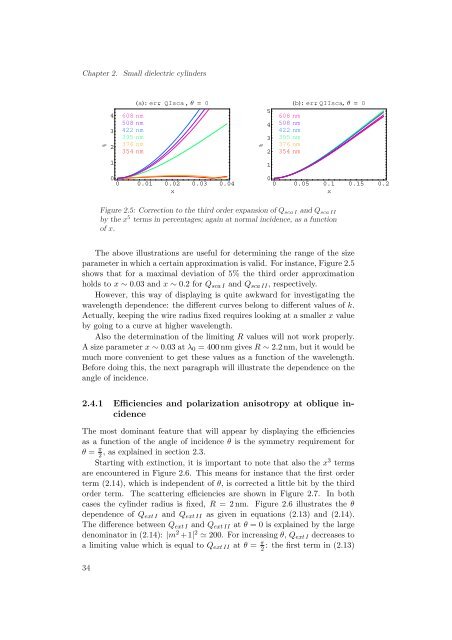
Chapter 2.Small dielectric cylinders%432608 nm508 nm422 nm395 nm376 nm354 nma:err. QIsca,Θ ⩵ 0%5432608 nm508 nm422 nm395 nm376 nm354 nmb:err.QIIsca,Θ ⩵ 01100 0.01 0.02 0.03 0.04x00 0.05 0.1 0.15 0.2xFigure 2.5: Correction to the third order expansion of Q sca I and Q sca IIby the x 5 terms in percentages; again at normal incidence, as a functionof x.The above illustrations are useful for determining the range of the sizeparameter in which a certain approximation is valid. For instance, Figure 2.5shows that for a maximal deviation of 5% the third order approximationholds to x ∼ 0.03 and x ∼ 0.2 for Q sca I and Q sca II , respectively.However, this way of displaying is quite awkward for investigating thewavelength dependence: the different curves belong to different values of k.Actually, keeping the wire radius fixed requires looking at a smaller x valueby going to a curve at higher wavelength.Also the determination of the limiting R values will not work properly.A size parameter x ∼ 0.03 at λ 0 = 400 nm gives R ∼ 2.2 nm, but it would bemuch more convenient to get these values as a function of the wavelength.Before doing this, the next paragraph will illustrate the dependence on theangle of incidence.2.4.1 Efficiencies and polarization anisotropy at oblique incidenceThe most dominant feature that will appear by displaying the efficienciesas a function of the angle of incidence θ is the symmetry requirement forθ = π 2, as explained in section 2.3.Starting with extinction, it is important to note that also the x 3 termsare encountered in Figure 2.6. This means for instance that the first orderterm (2.14), which is independent of θ, is corrected a little bit by the thirdorder term. The scattering efficiencies are shown in Figure 2.7. In bothcases the cylinder radius is fixed, R = 2 nm. Figure 2.6 illustrates the θdependence of Q ext I and Q ext II as given in equations (2.13) and (2.14).The difference between Q ext I and Q ext II at θ = 0 is explained by the largedenominator in (2.14): |m 2 +1| 2 ≃ 200. For increasing θ, Q ext I decreases toa limiting value which is equal to Q ext II at θ = π 2: the first term in (2.13)34