The Numerical Simulation of Nonlinear Waves in a Hydrodynamic ...

THE NUMERICAL SIMULATION OFNONLINEAR WAVES IN AHYDRODYNAMIC MODEL TEST BASINJaap-Harm Westhuis

Copyright c○ 2001 by Jaap-Harm Westhuisprinted by ...ISBN ...Figure cover: photograph of the Seakeeping and Manoeuvering Basin at MARIN(Wageningen, The Netherlands) merged with a graph of measured (solid line) andsimulated (dots) wave elevation using the algorithm of this thesis.This thesis was typeset using L A TEX2ε.

THE NUMERICAL SIMULATION OFNONLINEAR WAVES IN AHYDRODYNAMIC MODEL TEST BASINPROEFSCHRIFTter verkrijging vande graad van doctor aan de Universiteit Twente,op gezag van de rector magnificus,prof.dr. F.A. van Vught,volgens besluit van het College voor Promotiesin het openbaar te verdedigenop vrijdag 11 mei 2001 te 16:45 uurdoorJaap-Harm Westhuisgeboren op 23 augustus 1973te Amsterdam.

Dit proefschrift is goedgekeurd door de promotorprof.dr.ir. E.W.C. van Groesen(Faculteit der Toegepaste Wiskunde)

AbstractThis thesis describes the development of a numerical algorithm for the fully nonlinearsimulation of free surface waves. The aim of the research is to develop, implementand investigate an algorithm for the deterministic and accurate simulation of twodimensional nonlinear water waves in a model test basin. The simulated wave fieldmay have a broad banded spectrum and the simulations should be carried out by anefficient algorithm in order to be applicable in practical situations. The algorithmis based on a combination of Runge-Kutta (for time integration), Finite Element(boundary value problem) and Finite Difference (velocity recovery) methods. Thescheme is further refined and investigated using different models for wave generation,propagation and absorption of waves.The accuracy and stability of the numerical scheme are investigated and the numericaldispersion error is determined for several discretisation parameters. It was found thatstable, second order accurate discretisations can be obtained using first order FiniteElements and second order Finite Differences. The results also showed that a globalprojection method, using Finite Elements for velocity recovery, results in unstablediscretisations. By a suitable choice of the grid density parameter the dispersionerror of a small amplitude regular numerical wave can be annihilated by cancellationof errors. A physically relevant error measure for broad banded wave simulations isintroduced and mass and energy conservation show to be sufficiently small for accuratesimulations.Wave generation methods based on models of physical wave makers and methods fornumerical wave generation are described and evaluated. The discrete wave boardtransfer functions for flap- and piston-type wave generators are determined and itis concluded that the numerical wave generator produces slightly higher waves thanexpected from continuous analysis. It was also found that application of the algorithmto wave simulation may result in unstable discretisations for specific geometries incombination with certain numerical grids.Measurements that were performed on the reflection properties of beaches in themodel basin are compared to a numerical wave absorption method. The introducedabsorption method consists of combined pressure damping, horizontal grid stretchingand application of a Sommerfeld condition. Strict energy decay is guaranteed and thecombination allows for effective absorption for a broad range of frequencies. Reflectionvii

coefficients smaller than 0.7 % can be achieved at relative low computational cost. Itis also shown that by suitable choice of parameters the combined absorption methodcan reasonably approximate the measured reflections on artificial beaches in the basin.The algorithm was further applied to several benchmark tests confirming the validityof the results. Also the direct comparison with measurements showed satisfactoryagreement.The numerical scheme was used to investigate the long time evolution of nonlinearwave groups. The efficiency and accuracy of the algorithm allowed to explore thedynamics of these waves on an unprecedented time and spatial scale. This has led todetailed information and new insights in the long time evolution of bichromatic wavegroups and served as a basis for further experimental and analytical investigations.A study on the propagation of a confined wave group over a bottom topography,the disintegration of a confined wave train and an elaborate study involving numerousmeasurements and simulations on the evolution of bichromatic wave groups arepresented. The disintegration of a wave train in groups has been observed, but thecomplete splitting into clearly separated groups can not be rigorously confirmed bythe numerical results. Investigation of the evolution of a confined (NLS-soliton) wavegroup over a bottom topography showed the defocussing of the group and the generationof a large free solitary wave. The long time evolution of bichromatic wavesshowed spatial periodic variations of the wave spectrum, indicating recurrence. Anappropriate scaling was experimentally constructed that relates the ratio of amplitudeand original frequency difference (∆ω/q) to the observed spatial recurrence periods.Examination of the envelope evolution of the bichromatic waves show the splittingof the original envelope in two distinguishable envelopes. These distinguished groupsare observed to interact in at least two qualitatively different ways, both showingenvelope recurrence.viii

PrefaceSince the spring of 1997 I have enjoyed the freedom of doing research in the topic ofmy choice. This opportunity was given to me by the combined effort of my promotorprofessor Brenny van Groesen (University of Twente) and René Huijsmans, seniorresearcher at the Maritime Research Institute Netherlands (MARIN ). I greatly appreciatetheir efforts and support, and their flexibility to grant me the freedom indoing some unrelated research. The PhD position was financed by the KNAW (RoyalNetherlands Academy of Arts and Sciences) under grant number 95-BTM-29 (Lab-Math) and the additional financial support from MARIN is acknowledged.During this project I was stationed at MARIN , Wageningen. There I have enjoyedthe company of many (PhD-)students from different nationalities, many who I stillfrequently encounter. I would like to thank all of them for their pleasant companyand cheerful moments. The last years bear the most fresh memories and during thistime I have had the pleasure of having three distinctly different personalities as roommates. I would like to thank Albert Ballast, Anne Boorsma and Jie Dang for thefine discussions, meals and ’sporting events’ that made up a significant part of ourworkday.A special word of thanks is addressed to Andonowati, Agus Suryanto, Helena Margeretha,Edi Chayono and Robert Otto who have actively participated in the researchprogram LabMath and whose contributions and discussions provided valuable materialfor my research. Although most of my time was spent at MARIN , I frequentlyvisited the Department of Mathematics at the University of Twente. I have enjoyedthe conversations with Wilbert, Timco, Barbera, Stephan and Frits and wishto express my special thanks to the help and support from the secretaries: Marielle,Miranda and Carole.The last years, working hours have taken up a large part of the week. The remainingtime that I spent with friends and family have given me great pleasure and knowledgethat can not be found in text books. I want to thank my two paranimfs, Rogier andJasper, for their friendship and efforts, but most of all I want to thank Aster...ixZeist, 13-02-2001Jaap-Harm Westhuis

ContentsAbstractPrefaceNotationsviiixxiii1 Introduction 11.1 A hydrodynamic laboratory . . . . . . . . . . . . . . . . . . . . . . . . 11.2 Numerical simulation of nonlinear waves . . . . . . . . . . . . . . . . . 41.3 Contents and outline of the thesis . . . . . . . . . . . . . . . . . . . . . 62 Mathematical Model and Numerical Algorithm 152.1 Mathematical model . . . . . . . . . . . . . . . . . . . . . . . . . . . . 152.1.1 Field equations . . . . . . . . . . . . . . . . . . . . . . . . . . . 162.1.2 Free surface boundary conditions . . . . . . . . . . . . . . . . . 172.2 Numerical algorithm . . . . . . . . . . . . . . . . . . . . . . . . . . . . 202.2.1 Free surface . . . . . . . . . . . . . . . . . . . . . . . . . . . . . 202.2.2 Time stepping . . . . . . . . . . . . . . . . . . . . . . . . . . . 232.2.3 Field method vs. Boundary Integral method . . . . . . . . . . 25General heuristic comparison . . . . . . . . . . . . . . . . . . . 27Numerical Wave Tank example . . . . . . . . . . . . . . . . . . 28Recent developments . . . . . . . . . . . . . . . . . . . . . . . 292.2.4 Finite Element Method . . . . . . . . . . . . . . . . . . . . . . 30Weak formulation . . . . . . . . . . . . . . . . . . . . . . . . . 30The use of higher order FE’s . . . . . . . . . . . . . . . . . . . 322.2.5 Velocity recovery . . . . . . . . . . . . . . . . . . . . . . . . . . 33Global projection method . . . . . . . . . . . . . . . . . . . . . 34Finite Difference recovery of the velocity . . . . . . . . . . . . . 352.3 Implementation . . . . . . . . . . . . . . . . . . . . . . . . . . . . . . . 372.4 Scope of the investigations . . . . . . . . . . . . . . . . . . . . . . . . . 38xi

3 Simulation of Free Surface Waves 413.1 Linear and non-linear wave models . . . . . . . . . . . . . . . . . . . . 423.1.1 Progressive periodic linear waves . . . . . . . . . . . . . . . . . 423.1.2 Nonlinear progressive wave models . . . . . . . . . . . . . . . . 443.2 Accuracy and stability . . . . . . . . . . . . . . . . . . . . . . . . . . . 463.2.1 Numerical grid . . . . . . . . . . . . . . . . . . . . . . . . . . . 473.2.2 Stability Analysis . . . . . . . . . . . . . . . . . . . . . . . . . . 49Discretised equations . . . . . . . . . . . . . . . . . . . . . . . 50Stability of the spatial discretisation . . . . . . . . . . . . . . . 52Stability of the time integration . . . . . . . . . . . . . . . . . 56Conclusions . . . . . . . . . . . . . . . . . . . . . . . . . . . . 603.2.3 Grid refinement . . . . . . . . . . . . . . . . . . . . . . . . . . . 603.3 Dispersion relation . . . . . . . . . . . . . . . . . . . . . . . . . . . . . 623.3.1 Dispersion error σ . . . . . . . . . . . . . . . . . . . . . . . . . 633.3.2 Minimisation of σ(1/4, 4) . . . . . . . . . . . . . . . . . . . . . 65Floating point operations . . . . . . . . . . . . . . . . . . . . . 65Uniform grid . . . . . . . . . . . . . . . . . . . . . . . . . . . 67Nonuniform grid . . . . . . . . . . . . . . . . . . . . . . . . . 693.4 Mass and energy conservation . . . . . . . . . . . . . . . . . . . . . . . 713.5 Applications . . . . . . . . . . . . . . . . . . . . . . . . . . . . . . . . . 753.5.1 Comparative study on a sloshing wave . . . . . . . . . . . . . . 753.5.2 Solitary wave propagation over uneven bottoms . . . . . . . . . 763.6 Conclusions . . . . . . . . . . . . . . . . . . . . . . . . . . . . . . . . . 834 Simulation of Wave Generation 854.1 Flap- and piston-type wave maker . . . . . . . . . . . . . . . . . . . . 864.1.1 Linear model . . . . . . . . . . . . . . . . . . . . . . . . . . . . 864.1.2 Numerical modelling . . . . . . . . . . . . . . . . . . . . . . . . 88Grid points on the wave maker . . . . . . . . . . . . . . . . . 92Free surface grid points . . . . . . . . . . . . . . . . . . . . . . 924.1.3 Grid convergence . . . . . . . . . . . . . . . . . . . . . . . . . . 934.1.4 Linear analysis . . . . . . . . . . . . . . . . . . . . . . . . . . . 94Discretised equations . . . . . . . . . . . . . . . . . . . . . . . 95Intersection point . . . . . . . . . . . . . . . . . . . . . . . . . 984.2 Wedge wave maker . . . . . . . . . . . . . . . . . . . . . . . . . . . . 1014.2.1 Analysis . . . . . . . . . . . . . . . . . . . . . . . . . . . . . . . 1034.2.2 Results . . . . . . . . . . . . . . . . . . . . . . . . . . . . . . . 1054.3 Numerical velocity generation . . . . . . . . . . . . . . . . . . . . . . . 1094.3.1 Combined flux-displacement wave maker . . . . . . . . . . . . 1094.3.2 Absorbing wave maker . . . . . . . . . . . . . . . . . . . . . . 1104.4 Conclusions . . . . . . . . . . . . . . . . . . . . . . . . . . . . . . . . . 113xii

6 Nonlinear Wave Groups 1656.1 Previous investigations . . . . . . . . . . . . . . . . . . . . . . . . . . . 1656.1.1 Modulated wave trains . . . . . . . . . . . . . . . . . . . . . . . 1666.1.2 Bichromatic waves . . . . . . . . . . . . . . . . . . . . . . . . . 1686.2 Confined wave groups . . . . . . . . . . . . . . . . . . . . . . . . . . . 169NLS coefficients . . . . . . . . . . . . . . . . . . . . . . . . . . 169Disintegrating wave trains . . . . . . . . . . . . . . . . . . . . 1716.2.1 Propagation over an even bottom . . . . . . . . . . . . . . . . . 1726.2.2 Propagation over a slope . . . . . . . . . . . . . . . . . . . . . . 1766.3 Bichromatic wave groups . . . . . . . . . . . . . . . . . . . . . . . . . . 1786.3.1 Measurements . . . . . . . . . . . . . . . . . . . . . . . . . . . 1796.3.2 Numerical simulations . . . . . . . . . . . . . . . . . . . . . . . 182Comparison with measurements . . . . . . . . . . . . . . . . . 187Prolongation of the domain . . . . . . . . . . . . . . . . . . . . 1896.3.3 Non stationarity . . . . . . . . . . . . . . . . . . . . . . . . . . 193Spatial period . . . . . . . . . . . . . . . . . . . . . . . . . . . 193Benjamin-Feir instability . . . . . . . . . . . . . . . . . . . . . 196Envelope evolution . . . . . . . . . . . . . . . . . . . . . . . . 2056.4 Conclusion and discussion . . . . . . . . . . . . . . . . . . . . . . . . . 2097 Conclusions and recommendations 213AppendicesA Equivalence of strong and weak formulation 219A.1 Sobolev spaces . . . . . . . . . . . . . . . . . . . . . . . . . . . . . . . 219A.2 Extended Green’s formula for the Laplace operator . . . . . . . . . . . 220A.3 Lax-Milgram theorem . . . . . . . . . . . . . . . . . . . . . . . . . . . 221A.4 Equivalence . . . . . . . . . . . . . . . . . . . . . . . . . . . . . . . . . 221B Details of the numerical methods 223B.1 Lagrangian interpolation and simplex coordinates . . . . . . . . . . . . 223B.2 Modified Butcher tables . . . . . . . . . . . . . . . . . . . . . . . . . . 227C Nondimensional wave quantities 229Bibliography 230Samenvatting 242Curriculum Vitae 243Index 241xiv

NotationsIn the table below, the notations used throughout this thesis are listed in alphabeticorder of their first symbol (first the notations starting with a Roman symbol then thenotations starting with a Greek symbol). Besides a short description of the notation,the section where the notation is introduced is given for further reference.Notations starting with a Roman symbola amplitude of a regular wave [section 3.1 ]āstroke amplitude of a wave board to generate a linear regular wavewith amplitude a [subsection 4.1.1]a w half breadth of the wedge wave maker [section 4.2]a(·, ·) bilinear form [subsection 2.2.4 and appendix A]A amplitude of the wave envelope [subsection 3.1.2 and section 6.2]AMatrix resulting from linearisation of the discretised equations [subsection3.2.2, subsection 4.1.4 and subsection 5.4.2]b(·, ·) bilinear form [subsection 2.2.4 and appendix A]bmatrix resulting from the linearisation of the discretisation of thedriving terms [subsection 4.1.4]c phase velocity of a regular wave [section 3.1]c g group velocity of a linear wave group [section 3.1]c s velocity parameter in the Sommerfeld condition [subsection 5.3.1]c.c.complex conjugated of the previous expressionC j coefficient of an evanescent mode [subsection 4.1.1]dparameter describing the geometry of a flap-piston wave maker [subsection4.1.1]d w depth of the wedge wave maker [section 4.2]Dindex set containing the node numbers associated with grid points onthe free surface [subsection 2.2.4]e measurement error in reflection coefficient [subsection 5.2.1]E discrete energy [section 3.4]xv

f(·) function defining the Dirichlet data on Γ D [section 2.2.4 and appendixA]˜f vector function containing the dynamic equations as q t = ˜f(q, t)[subsection 2.2.2]⃗F a force [subsection 2.1.1]g gravitational constant [subsection 2.1.1]g(·) function defining the Neumann data on Γ N [subsection 2.2.4 andappendix A]ĝvector containing the coefficients of the approximation of g(·) [subsection4.1.4].hthe water depthh grid grid refinement parameter [subsection 3.2.3]H wave height (crest to through distance) [subsection 3.1.2]H 1 (Ω) function space [subsection 2.2.4 and appendix A]H ±1/2 (Γ) function space [subsection 2.2.4 and appendix A]Iindex set containing the node numbers in V that do not belong to Dor S [subsection 2.2.4]k wavenumber of regular wave k = 2π/λ [subsection 3.1.1]˜kcomplex wavenumber of a linearly damped regular wave [subsection5.4.1]¯k averaged wavenumber in bichromatic wave [section 6.3]lparameter describing the geometry of a flap-piston wave maker [subsection4.1.1]Ltotal length of computational domainL Blength of beach without horizontal stretching of the grid [subsection5.3.3]L eff length of beach with horizontal stretching of the grid [subsection5.3.3]M discrete mass [section 3.4]⃗n vector normal to a surface (pointing outward) [subsection 2.1.2]nx number of nodes in horizontal direction [subsection 3.2.1]nz number of nodes in vertical direction [subsection 3.2.1]N iFinite Element base function associated with global node number i[subsection 2.2.4]Nindex set containing the node numbers associated with grid points onΓ N [subsection 4.1.4]p (fluid) pressure [subsection 2.1.1]p[F EM] polynomial order of the base functions used in the finite elementapproximation for Φ [subsection 3.2.2]p[F D] polynomial order on which the finite difference scheme to approximateΦ z is based [subsection 3.2.2]xvi

q¯qqamplitude of a single wave component in a regular waveflap stroke amplitude resulting in a wave amplitude q [subsection6.3.1]vector containing the discrete variables involved in time integration[subsection 2.2.2 and subsection 3.2.2]r reflection coefficient [subsection 5.2.1]R dispersion operator [subsection 5.4.1]⃗s vector tangential to a surface [subsection 2.2.5]Sindex set containing the node numbers associated with grid points onthe Sommerfeld boundary [subsection 5.4.2]S ′ surface tension [subsection 2.1.2]S 0 ′ linearised surface tension [subsection 3.1.1]t time [subsection 2.1.1]T wave period (T = 2π ω) [subsection 3.1.1]T mod modulation period (period of a wave group) [subsection 6.3.1]u horizontal velocity [subsection 3.1.2]⃗v fluid velocity vector [subsection 2.1.1]V index set containing all node numbers [subsection 3.2.2]x horizontal coordinate [subsection 2.1.1]z vertical coordinate [subsection 2.1.1]Notations starting with a Greek symbolα(x) coefficient of the pressure damping term α(x)Φ z [subsection 5.3.2]α i polynomial coefficients of α(x) = α 0 + α 1 x + α 2 x 2 [subsection 5.3.2]β parameter governing the vertical grid density [subsection 3.2.1]β ′ coefficient in front of the linear term A ξξ in the Non LinearSchrödinger equation [subsection 3.1.2 and section 6.2]γparameter governing the horizontal grid stretching in the dissipationzone [subsection 5.3.3]γ ′coefficient in front of the nonlinear term |A| 2 A in the Non LinearSchrödinger equation [subsection 3.1.2 and section 6.2]γ s surface tension coefficient [subsection 2.1.2]Γ boundary of the domain Ω [subsection 2.2.4 and appendix A]Γ Dpart of Γ on which Dirichlet data is specified [subsection 2.2.4 andappendix A]Γ Npart of Γ on which Neumann data is specified [subsection 2.2.4 andappendix A]δ small perturbation parameter (h/λ) 2 [subsection 3.1.2]δ ′relative frequency of modulation disturbance ω′ −ωω[subsection 6.3.3]xvii

∆k wavenumber difference in bichromatic wave [section 6.3]∆t discrete time step [subsection 2.2.2]∆x horizontal mesh width [subsection 3.2.2]∆z vertical mesh width [section 3.2.1]∆ω frequency difference in bichromatic wave [section 6.3]∆T period difference in bichromatic wave [section 6.3]ɛ perturbation parameter a/h [section 3.1.2]ε perturbation parameter ka [section 6.2]ξ slow spatial variable in moving frame of reference ξ = ε (x − c g t)[subsection 3.1.2 and section 6.2]η function describing the free surface elevation [subsection 2.1.2]ˆηvector containing the z-coordinate of the boundary nodes on the freesurface [subsection 3.2.2]θ phase function [subsection 3.1.2]λ wavelength (λ = 2π k) [subsection 3.1.1]µ eigenvalue of A [subsection 3.2.2]˜µ zero’th order approximation of the dispersion operator R. Rφ ≈ ˜µ · φ[subsection 5.4.1]µ ′ dynamic viscosity [subsection 2.1.1]ν kinematic viscosity [subsection 2.1.1]∇gradient operator. ∇ = (∂ x1 , . . . , ∂ xn ) T , where n is dimension of thespatial domain X of the function ϑ (x ∈ X; t) on which ∇ operates.ρ fluid density [subsection 2.1.1]σrelative phase velocity error resulting from discretisation [subsection3.3.1]ˆσParameter controlling the length of the tangential free surface gridcorrection vector [subsection 2.2.1]σ(a, b) maximum value of σ for a ≤ λ ≤ b. [subsection 3.3.2]τ slowly varying time τ = ε 2 t [section 6.2]φ linear free surface potential [subsection 5.3.2]ϕvector containing the potential values at the discrete grid points.An additional superscript denotes a restriction of ϕ to the index setsymbolised by the superscript.Φ velocity potential [subsection 3.2.2]ˆΦ discrete approximation of Φ [subsection 2.2.4]Ψ acceleration potential Ψ = Φ t [section 4.2]ω regular wave frequency [subsection 3.1.1]¯ω averaged frequency in bichromatic wave [section 6.3]Ω open domain inR d , d = 2, 3 [section 2.1].̂Ω discrete approximation of Ω. [subsection 2.2.4]⃗Ω fluid vorticity Ω ⃗ = ∇ × ⃗v [subsection 2.1.1]xviii

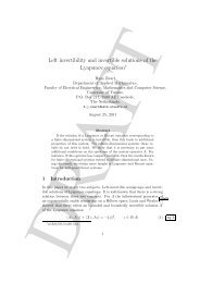
Chapter 1Introduction1.1 A hydrodynamic laboratoryA hydrodynamic laboratory is a complex of facilities in which maritime structuressuch as freight carriers, ferries and oil riggs are tested on a model scale. Beforethe actual construction, owners and designers need precise information about thehydrodynamic properties of their design. Questions as whether or not the contractvelocity of the design will be achieved are answered by testing in a model test basin.Other important aspects such as safety, maneuverability and controllability can alsobe investigated at this stage.A hydrodynamic laboratory usually has several facilities that are used for differenttesting purposes. When the hull resistance of a ship needs to be determined, a modelis towed through still water. To obtain information about dynamic properties suchas the stability and e.g. the maximum roll angles, model tests are performed ina seakeeping basin. In a seakeeping basin waves and possibly wind are generatedwhile the ship is kept at a fixed position or sails through the tank. Although thereare situations were the ship is towed by a carriage, most of the model tests areperformed by self propulsion. These models have active rudders, stabilising fins orpropellers that should allow for a steady course through the basin, while the carriagemoves over the model and facilitates the measurements . These towing tanks areusually narrow basins and do therefore not allow for simultaneous maneuverabilitytesting. The new SMB (Seakeeping and Manoeuvering Basin) at MARIN (MaritimeResearch Institute Netherlands) has the unique capability to combine manoeuveringand seakeeping model tests (Fig. 1.1 on the following page). The construction ofthe SMB started in 1998 and was operational in mid 1999. It is a 170x40x5 meterwater basin with 330 individually controlled wave maker segments on two sides andartificial beaches on the opposing sides. A giant carriage spanning the 40 meterwidth can follow a vessel sailing through the basin at a maximum speed of 6 [m/s].1

2 IntroductionFigure 1.1: The new Seakeeping and Manoeuvering Basin (SMB) at MARIN , Wageningen.The individual controllable segments of the wave maker on thelong side are clearly visible on the foreground.To evaluate the hydrodynamic properties of the ship the reaction of the vessel to acertain external force is measured. In seakeeping tests one is mainly interested in theship motions and forces due to loads caused by waves .In order to meaningfully test their ship, designers need to specify in what wave conditionsthe ship should be tested. A ferry operating solely in the North Sea betweenEngland and the Netherlands does not need to be tested for tropical hurricane waves.Every geographical area has its own wave characteristics, which are captured in a lowdimensional model with the significant period (T s ) and the significant wave height(H s ) as the most important dimensions. At the basis for these low dimensional modelsis most of the time a ’linear’ interpretation of reality. The waves are thought toconsist of a summation of regular waves and the parameters governing the dynamicsof ships are thought to have a linear dependence on the amplitude of the waves.Although for many situations this is an accurate and useful model of reality, it doesnot adequately describe extreme situations in which nonlinear interactions betweenwaves significantly influence the wave field . Model testing under extreme conditionsis however becoming more and more relevant for designers. Besides the generationof waves for regular testing in ’linear seas’ it therefore becomes increasingly importantto be able to generate extreme wave conditions at a prescribed position in thetank. To generate these conditions, accurate wave generation hardware and steeringalgorithm’s are essential. The new facilities of MARIN are equipped with sufficientlyaccurate hardware. Every segment of the wave maker is controlled by an individualelectric engine allowing for precise control of the wave board position.In 1997 the Mathematical Physics group of the department of Mathematics at the

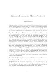
A hydrodynamic laboratory 3Figure 1.2: Relation between the different components of the LabMath project.University of Twente together with MARIN and the Indonesian Hydrodynamic Laboratory(IHL) started the LabMath program. The aim of this program was to developapplicable mathematics for the better controllability of the wave and current generationat hydrodynamic laboratories. The program consisted of four projects: (i) thedevelopment of nonlinear surface wave models , (ii) experimental wave measurementtechniques, (iii) modelling and simulation of wave-current interaction and (iv) fullynonlinear numerical simulation of waves in a basin.The relation between these projects is schematically depicted in the Fig. 1.2. Assumethat a specified spatial temporal wave pattern η(x i , t) in the basin is desired. By usinga suitable (nonlinear) surface model , a steering signal for the wave makers is derived.Then, a fully numerical simulation is used to investigate whether or not the proposedsteering signal will produce the desired wave characteristics. If not, the steering signalto the wave maker has to be adapted and the new signal can again be numericallyevaluated. Finally the steering signal is send to the wave makers in the physical basinand measurements must show whether or not the specified spatial-temporal pattern isindeed produced. If this process would have been performed by trial and error in thephysical basin, valuable tank-time would have been consumed. The fully numericalsimulation also allows for easy parameter variation studies and the wave data is availableon a fine spatial-temporal resolution, not achievable by measurement techniquesin the physical basin. This high resolution data can be used for the developmentand validation of simplified free surface models . It is stressed however, that continuouscross validation with physical experiments is essential and that the validitylimits of the models should always be carefully examined. The measurements thatare performed in the model test basin are also used to provide information for thedevelopment of the mathematical models that describe the artificial beaches and thewave-current interaction.The efforts of the LabMath project have been focused on two-dimensional (depth andlongitudinal direction) flow in the model basin. Follow-up research projects to extentthe results and numerical algorithm’s to a three dimensional basin have been granted.

4 IntroductionPreliminary results of the three dimensional simulations, performed by the author,showed promising results and indicated that the algorithm can indeed be effectivelyused for 3d wave simulations. As part of the LabMath project Eddy Cayhono isworking on nonlinear surface models (see e.g. van Groesen et al. (2001)) and HelenaMargeretha researches mathematical models that describe wave current interaction(see e.g. Margeretha et al. (2001)). Some aspects of the measurement techniqueshave been treated in Westhuis (1997) and further research and development on thesetechniques was performed by MARIN .This thesis reports on the development of the numerical algorithm for fully nonlinearsimulation of waves in a two-dimensional model basin. In summary, the aim of thisresearch project was to develop, implement and investigate an algorithm for the (i)deterministic and accurate simulation of (ii) two dimensional nonlinear waves (nobreakers) (iii) synthesised from a broad banded spectrum (iv) in a hydrodynamicmodel test basin (v) by an efficient algorithm allowing simulations to be performedin overnight jobs.We conclude this section by quoting prof. Bernard Molin who was the invited speakerfor the 22nd George Weinblum Memorial Lecture (Molin (1999)): ”As the oil industrymoves into deeper waters, the need for cross-validation of results from numerical codesand model tests becomes more acute. In 1000 or 2000 m water depths, it is notpossible to test a complete production system (FPSO + risers and moorings) at anappropriate scale, and a combined use of numerical software and model test resultsbecomes necessary. This means that the wave systems produced in the numerics andin the tank must be perfectly known and controlled. If they cannot be made to beidentical, then one should know how to manage the numerical and experimental toolsto cope with their differences.”1.2 Numerical simulation of nonlinear wavesThe numerical simulation of nonlinear waves follows from the mathematical modelthat is used to describe the wave dynamics. Based on the continuum hypothesis, theconservation of mass and momentum lead to the Navier-Stokes equations for the fluidvelocity and density. These equations simplify to Euler’s equations for the velocityif the fluid is considered incompressible and inviscous. An additional assumption onthe irrotationality of the fluid allows for the introduction of a velocity potential thatcompletely determines the velocity field (potential flow model). Under the conditionsleading to the potential flow model, the equations that describe the evolution ofthe air-water interface can be expressed in terms of the potential and the shape ofthe interface itself. Further assumptions on the shape of this surface and the waterdepth lead to numerous free surface models , in which all quantities are restrictedto the free surface. As will be motivated in section 2.1 the potential flow modelprovides an adequate description for the surface dynamics for nonlinear water waves.The assumptions leading to the more simple surface models conflicts with the design

Numerical simulation of nonlinear waves 5criteria mentioned at the end of the previous section. It is however stressed thatfor specific situations, surface wave models can accurately describe (nonlinear) wavedynamics.The numerical simulation of nonlinear water waves using the potential flow assumptionhas been studied since the mid 1970’s. Longuet-Higgins & Cokelet (1976) werethe first to simulate an asymmetric overturning deep water wave. They used a conformalmapping approach with space periodic boundary conditions and an artificialpressure distribution to enforce the breaking. Since then, many researchers have takenup the topic of nonlinear wave simulation, often in combination with wave-body interaction.Extensive reviews on the topic of wave simulation are given by Yeung(1982) and Tsai & Yue (1996). More recently Kim et al. (december, 1999) reviewedthe research on the development of Numerical Wave Tanks (NWT’s). In a NWT,the emphasis is both on wave simulation and wave-body interaction and aims at thereplacement (not simulation) of an experimental model basin (also called ExperimentalWave Tank). Because of the availability of these extensive and recent reviews,no literature overview is presented here. References are given throughout this thesiswhen appropriate.Most numerical methods for potential flow wave simulation are based on the mixedEulerian-Lagrangian method (employed by Longuet-Higgins & Cokelet (1976)) toseparate the elliptic Boundary Value Problems (BVP) from the dynamic equationsat the free surface. The fast majority of available numerical scheme’s that simulatefree surface potential flow, approximate the BVP using a Boundary Integral (BI)formulation. This formulation is then discretised using Boundary Elements (BE) (e.g.Dommermuth et al. (1988) [2d constant panel method], Romate (1989) [3d secondorder panel method], Grilli et al. (1989) [2d higher order boundary elements] andCelebi et al. (1998) [3d desingularised BI]. Other methods to solve the BVP are FiniteDifference [FD] and Finite Element [FE] methods to discretise the field equations. InFD methods (e.g. Chan (1977) and DeSilva et al. (1996)) the geometry is usuallymapped to a rectangular domain to efficiently implement the numerical scheme. Thisis not necessary for the FE methods, but although the FE method has been widelyused in steady state (viscous) flow problems and linearised free surface problems(e.g. Washizu (1982)) it did not receive much attention in nonlinear potential flowproblems until recently (e.g. Wu & Eatock Taylor (1994) [fixed walls] and Cai et al.(1998) [fixed walls and mapping to a rectangular domain]). The use of FE methodsin viscous numerical free surface simulation was also recently reported by Braess &Wriggers (2000). Finally, the spectral method based on a Taylor expansion of theDirichlet-Neumann operator developed by Graig & Sulem (1993) is mentioned as analternative to the BE, FD and FE methods. For numerical studies involving wavebreaking in potential flow we refer to Vinje & Brevig (1981), Dommermuth et al.(1988), Banner (1998) and Tulin & Waseda (1999) [experimental data and numericalsimulations] and Guignard et al. (1999) [shoaling of solitary wave]. Many authors(e.g. Longuet-Higgins & Cokelet (1976) [BE], Dold (1992) [BE], Wu & Eatock Taylor(1994) [FE] and Robertson & Sherwin (1999) [FE]) report on the appearance of sawtoothinstabilities during numerical simulation. In order to simulate over sufficiently

6 Introductionlong time, additional smoothing of the intermediate results or regridding is used toavoid numerical instabilities.The numerical algorithm and implementation presented in this thesis differs from thepreviously reported scheme’s in the combination of the following aspects:• a direct (no mapping) field discretisation of the successive boundary value problemsusing a Finite Element method with a successive velocity recovery usingFinite Differences.• marginally stable linearised spatial discretisation due to the combination ofFinite Elements and Finite Differences (no smoothing necessary).• the inclusion in the numerical simulation of a model for artificial beaches thatare used in the experimental wave tank.• a focus on the simultaneous accurate simulation of nonlinear waves of differentwavelength on a single numerical grid.• a modular, object oriented algorithm for the implementation of the geometry,allowing for the separated development, implementation and testing of e.g. wavemakers and numerical beaches.1.3 Contents and outline of the thesisThis section describes the main contents of the thesis and serves as an outline forquick reference to the appropriate (sub)sections. The results of the investigationshave been ordered as follows. After chapter 2 describes the mathematical modeland numerical algorithm, chapter 3 investigates the numerical simulation of waveswithout the influence of artificial wave generation and/or absorption. These lattertwo topics are consecutively treated in chapter 4 and chapter 5. In chapter 6 thenumerical algorithm is used to investigate the long time evolution of wave groups andthe final chapter 7 contains some concluding remarks and some recommendations forfurther research. The appendices contain the sketch of a proof on the equivalence oftwo problems, some details of the numerical method and a graph relating the basiclinear wave quantities. This latter graph may be of practical use for the physicalinterpretation of non-dimensionalised results. After the appendix and a bibliographyand index are provided that can be used for further reference and navigation throughthe thesis.Many of the captions of the figures in this thesis contain a list of numerical parametersthat were used to perform the presented simulation from which the presented resultshave been derived. Although this might distract the reader from the intention of thefigure, this data is provided to improve repeatability of the numerical simulations byother researchers. An important aim of the presentation of the research has been toprovide sufficient information for complete reconstruction of all presented results.

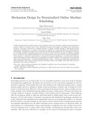
Contents and outline of the thesis 7In the following subsections the content of chapters 3-6 is summarised. The firstparagraph of each section contains a brief abstract describing the structure of thechapter in relation to its section division. The next paragraphs in the subsectiondiscuss the contents of the chapter in more detail and in relation to its subsectionstructure.Chapter 2 - governing equationsThe aim of this chapter is to introduce the equations that describe the free surface dynamics[2.1], the numerical algorithms to approximate the solution of these equations[2.2] and the implementation of this algorithm in a computer code [2.3].In section 2.1 the field equations describing potential flow are derived [2.1.1] and theassumptions leading to these equations are motivated. The equations governing thefree surface dynamics are next derived [2.1.2] resulting in the final set of governingequations. Section 2.2 starts by describing the numerical treatment of the free surface[2.2.1] and the resulting structure of the top-level time-marching scheme [2.2.2]. Thistime marching scheme consists of the repeated construction and solution of a boundaryvalue problem followed by a velocity recovery step. The use of field methods versusboundary integral methods to solve the boundary value problems are compared [2.2.3]and based on this comparison the choice for the Finite Element Method is motivatedand further discussed in detail [2.2.4]. For the velocity recovery methods [2.2.5] a globalprojection method and finite differences are discussed.The chapter ends with some brief comments on the object oriented structure of theimplementation in section 2.3 and the definition of the scope of the investigations insection 2.4 for chapters 3,4 and 5.Chapter 3 - free surface wavesThe focus of chapter 3 is on the analysis of the numerical methods introduced in theprevious chapter with respect to free surface waves in a basin with natural boundaries.After a brief introduction of some relevant equations for the description of(nonlinear) wave propagation [3.1] the accuracy and stability of the numerical schemeare investigated [3.2]. To further quantify the numerical errors and the effect of thediscretisation parameters, the error of the discrete dispersion relation is established[3.3]. The stability and error analysis of the previous sections are mainly based onthe linearisation of the discretised equations. In order to asses the accuracy of thefully nonlinear discretisation, the discrete mass and energy conservation is investigated[3.4]. The chapter ends with some applications [3.5] and the conclusions [3.6] ofthis chapter.In section 3.1 the linearised free surface equations and the resulting dispersion relationfor linear waves [3.1.1] are derived. Next, the deep water Stokes waves and the Boussi-

8 Introduction(a) Spatial-temporal grid refinement forfirst order Finite Elements and second orderFinite Differences. The graphs showsa decay of the energy norm error proportionalto h −2grid .(b) The σ = 0 curve connects the valuesof the grid density parameter β for whichthe phase velocity of the linearised discretisationequals the exact linear phasevelocity.Figure 1.3: Two figures from chapter 3. (a) Grid refinement study in subsection 3.2.3on page 60. (b) analysis of discrete dispersion relation in subsection 3.3.1on page 63.nesq, KdV and NLS equations [3.1.2] are introduced for future reference. Section 3.2starts with the introduction of the numerical gridding [3.2.1] and the introduction ofthe vertical grid density parameter β. The effect of this parameter and other numericalparameters on the stability of the numerical scheme is then investigated [3.2.2].First the spatial discretisation of the governing equations are linearised and a VonNeumann stability analysis is performed. The results show that scheme is marginallystable when Finite Differences are used as a velocity recovery method. The use of aglobal projection method can however lead to unstable spatial discretisations and istherefore rejected as a suitable method. Next the stability of the discretisation of thetime integration is investigated. The growth rates of eigenvectors due to 4 stage and5 stage Runge-Kutta methods are determined and compared when applied to the linearisedspatial discretisation. It is concluded that a 5 stage method is preferable overa 4 stage method. After these discussions on the stability of the linearised discretisedequations, the convergence of the nonlinear discretisation is investigated by a systematicgrid refinement study [3.2.3] showing that the numerical scheme is second orderaccurate (see also Fig. 1.3 on the preceding page). Section 3.3 starts by introducingthe relative dispersion error σ [3.3.1] and investigates the effect of the numerical gridon this parameter. It is shown that for a specified wavelength this error can be madezero due to cancellations (see also Fig. 1.3 on the page before). To investigate thequality of the simulation of a broad banded wave spectrum, the maximum error σ(a, b)over a range of wavelength on a single grid is introduced [3.3.2] and the effect of thenumerical parameters is examined. Analysis of the computational complexity of firstand second order FE implementations and extensive variations of the FD polynomialorders and other grid parameters result in a graph in which the minimal achievable

Contents and outline of the thesis 9σ(1/4, 4) error as a function of the computational effort is given. The results showthat by suitable choice of the nonuniform grid distribution and the FD polynomialorder, a reduction in the σ(1/4, 4) error of a factor 100 can be achieved given thesame computational effort. This allows for accurate simulations over realistic timescales of a complete wave basin in overnight jobs.To further investigate the quality of the nonlinear simulation, the effect of numericalparameter variations on the discrete mass and energy conservation is investigated insection 3.4. It is concluded that the discrete mass and energy are very slowly decreasingfunctions of time and are positively influenced by choosing the nonuniform gridconfigurations. The second last section 3.5 of this chapter describes two applicationsof the numerical method. The first application discusses the results of a benchmarkproblem on the evolution of a nonlinear sloshing waves [3.5.1]. The second applicationconcerns the simulation of the splitting of solitary waves over a bottom topography[3.5.2]. At the end of the chapter the conclusions of the investigations are summarised[3.6].Chapter 4 - wave generationChapter 4 is concerned with the numerical simulation of wave generation. A distinctionis made between wave generation methods based on models of physical wavemakers (such as flap- and piston-type [4.1] and heaving wedge [4.2] wave makers ) andmethods based on numerical velocity generation models [4.3].In section 4.1 the numerical simulation of flap- and piston wave makers is discussed.After a linear model describing both wave makers [4.1.1] is presented, the numericalmodelling is discussed in more detail [4.1.2]. The numerical gridding around the wavemaker and the treatment of the free surface grid points near the wave maker are examined.A small grid convergence study is performed [4.1.3] to investigate the correctimplementation of the numerical scheme. Similar to the linear analysis of chapter 3,the discretisation of the wave generator is constructed [4.1.4] and the discrete Biéseltransfer functions - relating the wave board stroke and the wave amplitude - are determined.Also, the wave envelope near the wave board that is largely determinedby evanescent modes, is determined from linear analysis and compared to continuousresults (see also Fig. 1.4 on the following page). It is concluded that even forrelative fine (with respect to previous chapter) horizontal and vertical numerical gridresolution, the discrete transfer function for high frequencies is overpredicted by thediscretisation. For accurate simulations, the discrete transfer functions should thereforebe used when wave board steering signals are synthesised from a target wavespectrum. Based on the linear analysis it is also shown that in the present formulation,the intersection grid point between the wave maker and free surface should betreated analogous to the free surface grid points.In section 4.2 the results on a comparative study on a forced heaving wedge wavemaker are presented. After some remarks on the computation of the force on the

10 IntroductionFigure 1.4: Comparison between the exact and a numerical solution of the (linear)wave envelope near the wave maker . Accurate representation of theevanescent modes is necessary to simulate the effects of nonlinear interactionsnear the wave maker (from subsection 4.1.4 on page 94)wetted wedge, a linear stability analysis [4.2.1] is performed on the discretisation.This study showed and erratic stability behavior that sensitively depends on thenumerical grid. The section on the wedge wave maker is concluded by presentingthe results of the comparison [4.2.2] with other numerical codes. In general goodmutual agreement was found between the fully nonlinear codes. Section 4.3 treatstwo practical numerical wave generation methods. First a combined flux-displacementwave maker is introduced [4.3.1] in which the wave generation is partially governedby wave board displacement and partially by numerical flux generation. The secondnumerical wave generation method implements a combined generating potential witha Sommerfeld condition [4.3.2] to absorb reflected waves with the same frequency asthe generated wave. It is shown by transient generation of a small standing wave thatthis is an adequate wave generator for small amplitude waves. This chapter on wavegeneration ends with the gathered conclusions [4.4] from the previous sections.

Contents and outline of the thesis 11Chapter 5 - wave absorptionThe main emphasis in chapter 5 is on the numerical simulation of wave absorption.First the absorption of waves in a hydrodynamic basin [5.1] is examined. Then themeasurements that were performed at the beaches of the new seakeeping and manoeuveringbasin at MARIN [5.2] will be presented. These measurements are latercompared to numerical wave absorption methods [5.3] and the most promising methodsare further analyzed [5.4]. The results of the simulations, analysis and measurementsare then compared and discussed [5.5].In section 5.1 a brief overview on passive [5.1.1] and active [5.1.2] wave absorbers ina physical basin is presented. Then, in section 5.2, the measurements that were performedon the concepts for the artificial beaches of the new SMB are treated. First themethod to determine the reflection coefficient (r.c.) [5.2.1] is described. This descriptionincludes the measurement setup and two different methods (envelope modulationand spectral decomposition) to extract the r.c.’s from the data. The results for twoartificial beaches are presented [5.2.2] that show relative large unexplained scatteringof the data probably caused by measurement and r.c. model assumptions.The next section 5.3 introduces several methods for numerical wave absorption. TheSommerfeld condition [5.3.1], the energy dissipation zone [5.3.2] based on pressuredamping, the horizontal grid stretching and their combination are discussed in moredetail. The combined absorption zone is expected to provide the most efficient androbust numerical wave absorption and it is shown that energy decay in this zone isguaranteed. The reflection coefficients of the combination are first determined by usinga continuous approximation [5.4.1] of the linearised equations for constant, linearand parabolic damping functions. This continuous analysis is based on a plane waveassumption and uses an approximation ˜µ for the dispersion operator R in the lineardamping zone. Next, the reflection coefficients are determined from analysis of thelinearised discretised equations [5.4.2]. The effect of the additional damping terms andSommerfeld condition on the discrete spectrum is determined and it is shown that theenvelope modulation method to determine the r.c.’s provides accurate results whenused in combination with the linearised discretised equations. The intersection pointbetween the free surface and the boundary on which the Sommerfeld condition isdefined is investigated and it is shown that artificial eigenvectors appear in the discretisation.Based on the analysis of these additional vectors it is concluded thatthe implementation of the intersection point as a Sommerfeld condition is preferableover the treatment of this point as a free surface particle. Following this discussion,the effect of the additional equations following from discretisation of the Sommerfeldcondition on the stability of the time integration is investigated. It is shown that theSommerfeld condition can impose a severe condition on the time step and that the localhorizontal mesh width ∆x 0 near the Sommerfeld boundary should be significantlylarger in order not to influence the stability of a simulation without a Sommerfeldcondition. Discrete analysis of the polynomial damping functions showed characteristicdifference in r.c.’s for constant and linear damping functions but similar results for

12 Introduction(a) Configuration to approximate atransparant beach. Reflection coefficientssmaller than 0.7% are achievedover a wide range of frequencies at thecost of extending the domain with twotimes the depth.(b) Configuration to approximate themeasured reflection coefficients. Thecombination of the stretching, dampingand Sommerfeld condition is usedto tune the numerical reflection curveto the measurements.Figure 1.5: Reflection coefficients from the combined absorbing zone developed inchapter 5. A distinction is made between a transparent numerical beach(subsection 5.5.2 on page 157) and the simulation of the artificial beachin a model test basin (subsection 5.5.3 on page 159).linear and parabolic damping functions. The combined effect of damping, stretchingand Sommerfeld condition showed that high frequency waves can significantly reflectfrom the stretched grid, but that this can be compensated by suitable choice of thedamping coefficient. The stretching allows for large damping zone’s with relative fewgrid points thus providing an efficient method.In section 5.5 the resulting estimates for the r.c. based on the analysis from previoussection is discussed. Comparison of the continuous approximations and the convergednumerical approximations [5.5.1] showed that for constant damping functionsgood mutual agreement is achieved for high frequency waves but that the continuousmodel generally gives higher r.c. estimates than the discrete results. As it hasbeen checked that the numerical results had converged the difference can only becontributed to the plane wave assumption underlying the continuous analysis. Forlinear damping functions the agreement between the continuous and discrete resultsis poor. Although both methods show the same trends, the quantitative differencesare large. It is shown that the result is quite sensitive to the dispersion operatorapproximation and it is thus concluded that this approximation in combination withthe plane wave assumption leads to wrong predictions of the reflection coefficients.Based on the discrete investigations, a combination of parameters is selected thatresults in minimal reflection coefficients [5.5.2] over the significant range of wavelengthat the computational cost of extending the domain with two times the depth (see alsoFig. 1.5). Through extensive parameter variation studies, a combination was selectedthat reasonably fits the scattered reflection coefficients that were previously measured[5.5.3] (see also Fig. 1.5). The chapter ends with section 5.6 in which the conclusions

Contents and outline of the thesis 13(a) Comparison of measurements (solidline), numerical simulations with the methodsof this thesis (dots) and linear theory(dotted line).(b) The nonlinear spatial evolution ofthe spectral components of a bichromaticwave (see subsection 6.3.2 on page 182and Fig. 6.15 on page 194).Figure 1.6: The evolution of nonlinear bichromatic wave groups.of this chapter are summarised.Chapter 6 - wave groupsIn chapter 6 the developed numerical scheme, including wave generation and absorptionis used to study the long time evolution of nonlinear wave groups. After anintroduction and a literature review [6.1] the propagation of confined wave group [6.2]over an uneven bottom topography is studied. Next, a more extensive study involvingnumerous measurements and simulations on the evolution of bichromatic wave groups[6.3] is presented. The conclusion of these investigations are summarised at the endof this chapter [6.4].In section 6.1 the literature on the evolution of modulated wave trains [6.1.1] andbichromatic waves [6.1.2] is reviewed. Section 6.2 then starts with the motivationfor the study of confined wave groups and introduces the coefficients governing theNonlinear Schrödinger (NLS) equation. A numerical simulation of a disintegratingwave train shows the splitting in solitary wave groups but the anticipated separationis not observed on the investigated time scale. Next, the construction of an initialsolution for the propagation of a confined solitary wave group [6.2.1] is investigated.The sub- and super harmonics that are freed when the first order component of theNLS solitary wave group solution is imposed are identified. After these additionalwaves have propagated sufficiently far from the main group, this group is isolatedand used for the investigation of the effect a depth variation [6.2.2]. The result of theincreasing depth is the freeing of a bound long wave and the defocussing of the wavegroup which transforms in a wave train on shallow water.Section 6.3 start with some notations used for the investigation of the evolution of

14 Introductiona periodically generated bichromatic wave group. First, a number of measurements[6.3.1] are presented that have been performed at the High Speed Basin at MARIN.These measurements clearly show the steepening of the waves at the front of thegroup of steep bichromatic waves. These measurements are then compared to numericalsimulations (that actually preceded the measurements) and excellent agreement[6.3.2] is observed (see also Fig. 1.6). To investigate the long time evolution, the dimensionsof the numerical basin are then stretched far beyond the realm of a physicalmodel basin. The spatial evolution of different energy modes are identified (see alsoFig. 1.6 on the preceding page) and the results of the numerical simulations are presentedin these low dimensional representations of the wave group evolution. Thenon-stationar behavior of the bichromatic wave group evolution is investigated [6.3.3]in three different ways. First the spatial recurrence period of the different modes isidentified and an appropriate scaling is found to unify the results. Next the relationwith the Benjamin-Feir instability of nonlinear deep water wave trains is examined.Although some correspondence is found, the growth factors of the side bands can notbe completely explained by this theory. Finally the evolution of the wave envelope isinvestigated. The results of the fully nonlinear numerical simulation are compared tosimulations using the NLS equation as an Initial Boundary Value Problem (IBVP).Opposed to the usual spatial periodic simulation of the NLS, the IBVP approach recoversthe asymmetric evolution and when corrected with the nonlinear Stokes groupvelocity, good quantitative agreement is found. Investigation of the wave group envelopeevolution form the fully nonlinear simulations, also showed two typically differentlong time envelope behavior, (i) the splitting of the original wave in two groups inwhich one is periodically overtaken by the other and (ii) the splitting in two wavegroupsin which the one periodically bounces between its neighboring groups. All theresults of these investigations on nonlinear wave group evolution are summarised inthe final section [6.4] of the chapter.

Chapter 2Mathematical Model andNumerical AlgorithmThe simulation of waves in a hydrodynamic model test basin requires four stages ofdevelopment. Firstly a mathematical model to describe the relevant physical processin the basin needs to be constructed, resulting in a set of governing equations . Next,these governing equations are either solved exactly or, when no exact solution isavailable, the solution of these equations is approximated using a numerical algorithm.Then this numerical algorithm needs to be implemented in a computer code andfinally the applicability of the numerical algorithm and the validity of the resultsneeds to be established. In this chapter the first three stages are described for thesimulation of free surface waves without addressing issues related to wave generationand absorption. These latter aspects and the numerical analysis and validation willbe dealt with in the subsequent chapters.2.1 Mathematical modelTo describe and investigate the evolution of waves in a laboratory, a mathematicalmodel is constructed. The mathematical model is based on the equations of fluidmechanics for which many classical textbooks, e.g. Lamb (1932) and Landau &Lifshitz (1987) are available. In this section the equations governing the dynamics ofwater with a free surface will be derived to introduce the notations and clarify theassumptions. The classical water-wave problem consists of solving the Euler equationsin the presence of a free surface. The field equations will be derived in subsection2.1.1. The nonlinear evolution of waves is governed by the boundary conditions atthe free surface which are introduced in subsection 2.1.2.15

16 Mathematical Model and Numerical Algorithm2.1.1 Field equationsThe two starting principles for the derivation of the equations of fluid mechanics arethe conservation of mass and conservation of momentum. The fluid velocity is denotedas ⃗v and is a function of the spatial variables and time. The density of the fluid isdenoted by ρ and is for the moment also assumed to be a function of space and time.Balancing the mass influx through the boundaries and the internal change of massinside a fixed control volume and taking the infinitesimal limits of this control volumeleads directly to the equation for conservation of mass∂ρ+ ∇ · (ρ⃗v) = 0. (2.1)∂tAs the fluid of interest is water and the compressibility (i.e. the relative change ofvolume per applied unit of pressure increment) of water equals 4.6 ·10 −10 , the densityis assumed constant and thus Eq. (2.1) reduces to∇ · ⃗v = 0. (2.2)The principle of conservation of momentum implies that in a control volume, movingwith the fluid flow, the change in momentum equals the total force acting on thecontrol volume. This principle is stated in Eq. (2.3).whered (ρ⃗v)dt= ⃗ F = ⃗ F i + ⃗ F g + ⃗ F f , (2.3)ddt = ∂ + ⃗v · ∇ (2.4)∂tdenotes the material derivative with respect to the fluid velocity. The forces actingon the control volume are⃗F i⃗F g⃗F f: inertia forces (−∇p),: gravitational force (ρ⃗g), with the gravitational, acceleration ⃗g = (0, 0, −g) T: frictional force due to tangential stresses.The frictional force ⃗ F f due to the tangential stresses is given by( ⃗ F f ) i = µ ′ ∇ · ∇⃗v i (2.5)where µ ′ is the dynamic viscosity (usually the dynamic viscosity is denoted by η butthis symbol is reserved for the free surface elevation function). Using the incompressibilityassumption and the resulting expressions for the total forces , Eq. (2.3) reducesto the Navier-Stokes equations for incompressible fluid flow,ρ d⃗v idt = −(∇p) i + µ ′ ∇ · ∇⃗v i + ρ⃗g i . (2.6)

Mathematical model 17To motivate further simplification of Eq. (2.6) the vorticity ⃗ Ω is introduced as⃗Ω = ∇ × ⃗v. (2.7)A velocity field is called irrotational if ⃗ Ω = 0. Taking the material derivative of ⃗ Ωand substitution of Eq. (2.6) results in Eq. (2.8).dΩ⃗ ( )dt = ⃗Ω · ∇ ⃗v + ν∇ · ∇Ω ⃗ (2.8)In Eq. 2.8), ν = µ′ρis called the kinematic viscosity. From Eq. (2.8) one can observethat in the absence of viscosity (i.e. µ ′ = 0) an initial irrotational velocity field((∇ × ⃗v) | t=0= 0) will remain irrotational for all time. Both for numerical simulationsas for experiments in the laboratory, the initial state of the velocity field is at rest (andthus irrotational), and therefore the velocity field will remain irrotational if viscouseffects are neglected.In the presence of viscosity but with an initial irrotational velocity field, diffusionwill mainly occur near the boundaries, because variations in the second derivative ofthe velocities will be largest there due to the no-slip boundary condition. However,the oscillatory nature of wave phenomena, ensures that the direction of the flowoften changes, so most of the inward diffusion will be restricted to a small boundarylayer. The distance of this Stokes boundary layer is of order O (√ )νω where ω isthe frequency of the wave motion in [ rads]. As the kinematic viscosity of water is oforder 10 −6 and the frequencies are typically of order 1, the boundary layer thicknessis of order 10 −3 . Therefore the viscous effect are considered negligible small withrespect to the wave lengths of interest (λ > /h > 1/4). However, when large secondorder spatial derivatives of the velocity occur (e.g. near breaking situations or otherviolent fluid motion) or very long time scales are considered, the inward diffusion maybecome significant. For references and applications of the simulation of low Reynoldsnumbers free surface flows, we refer to Tsai & Yue (1996).For an irrotational vector field ⃗v a scalar potential function Φ exists such that⃗v = ∇Φ. (2.9)Substitution of Eq. (2.9) in Eq. (2.1) leads to the Laplace equation for the potentialΦ,∇ · ∇Φ = 0. (2.10)In the next section the free surface will be introduced and the boundary conditionsat the free surface are derived.2.1.2 Free surface boundary conditionsAssume that the open domain Ω ⊂ R d has a boundary Γ that marks the fluid-airinterface. Free surface flow is usually considered as a limiting case of a two phase

18 Mathematical Model and Numerical Algorithmflow in which the dynamics of one phase (in this case air), are greatly simplified orignored. In this case, the velocity field of the air is considered zero and a constantatmospheric pressure is assumed. This leads to two conditions on the free surfaceinterface: kinematic and dynamic conditions.When the continuity equation Eq. (2.2) is integrated over a control volume Ω(t) whoseboundary S(t) moves in time we find∫∇(ρ⃗v)dΩ = 0 (2.11)Ω(t)and using Leibniz rule one derives∫− ρ drS dt∫S· ⃗ndS + ρ⃗v · ⃗ndS = 0 (2.12)where drdtrepresents the velocities with which the integration boundary moves. Denotingthese velocities by V ⃗ , the following condition for the boundary velocity can bedirectly obtained∫S(⃗v − ⃗ V ) · ⃗ndS = 0. (2.13)This condition states that the normal component of the fluid velocity has to equalthe normal component of the free surface velocity,⃗v n = ⃗ V n . (2.14)The introduced boundary normal ⃗n is defined as pointing outward of the fluid domainand ⃗ V n denotes the normal velocity of the boundary surface. The boundary conditionEq. (2.14) is a kinematic relation and therefore the condition, when applied to thefree surface, is usually referred to as the kinematic boundary condition.The second boundary condition follows from the continuity of the normal stresses overthe water-air interface, apart from contributions due to surface tension. If viscouseffects are neglected (as is assumed) this results in a relation between the pressuresof water and air and the forces due to surface tension,p water − p air = −S ′ . (2.15)The force due to the surface tension is proportional to the mean curvature of thesurface. If the surface is implicitly defined, this may be defined directly in terms ofthe two radii of curvature. When the surface is considered to be a function η(x, t) ofthe horizontal coordinates x and time, the mean curvature can be expressed in termsof derivatives of η as()S ′ ∇η= γ s ∇ · √ . (2.16)1 + |∇η|2

Mathematical model 19The factor γ s is called the surface tension and for water has a value of 7.3 10 −2 [N/m].It will be shown in section 3.1.1 that the effect of surface tension can be neglectedwith respect to the scales of interest. When Eq. (2.15) is applied to the free surface,it is referred to as the dynamic boundary condition. We will proceed by expressingthe kinematic and dynamic boundary conditions (2.14)-(2.15) in terms of the velocitypotential Φ.Substitution of the potential definition Eq. (2.9) in the Navier-Stokes equation Eq. (2.6),ignoring viscosity and expanding the total time derivative Eq. (2.4) results in∂∇Φ∂t+ (∇Φ · ∇) ∇Φ + 1 ∇p − ⃗g = 0 (2.17)ρwhich can be further simplified to( ∂Φ∇∂t + 1 2 |∇Φ|2 + p )ρ + gz = 0. (2.18)Integration of Eq. (2.18) results in the Bernoulli equation∂Φ∂t + 1 2 |∇Φ|2 + p + gz = f(t) (2.19)ρfrom which the integration constant f(t) can be eliminated by redefining Φ.Denoting η(x, t) as the free surface boundary between water and air, and substitutingEq. (2.15) in Eq. (2.19) the dynamic boundary condition on the free surface can bewritten as∂Φ∂t + 1 2 |∇Φ|2 + p air − S ′+ gη = 0 on z = η(x, t). (2.20)ρThe kinematic boundary condition Eq. (2.14) can also be formulated in terms of ηand Φ as∇Φ · [−η x , −η y , 1] = η t (x, t) on z = η(x, t) (2.21)which is usually denoted asη t = Φ z − η x Φ x − η y Φ y on z = η(x, t). (2.22)

20 Mathematical Model and Numerical AlgorithmAssuming the fluid to be incompressible and inviscid with an irrotational velocityfield and assuming the free surface boundary between water and air to be a singlevalued function of the horizontal coordinates and time, the following equationsgovern the motion of the free surface⃗v = ∇Φ(2.23a)∇ · ∇Φ = 0 in Ω (2.23b)∇Φ · ⃗n = V n on Γ (2.23c)(2.23d)∂Φ∂t + 1 2 |∇Φ|2 + p air − S ′+ gη = 0ρon z = η(x, t) (2.23e)η t = Φ z − η x Φ x − η y Φ y on z = η(x, t) (2.23f)For a treatment on the existence, uniqueness and regularity of a solution of the Laplaceboundary value problem on a domain with corners cf. e.g. Kawohl (1980). Wheninitial conditions for the potential and the free surface are added, equations (2.23)-(2.23) define a well defined initial value boundary problem for η and Φ.2.2 Numerical algorithmIn general no exact solution is available to equations (2.23)-(2.23). In these situations,discretisation methods can be used to find the solution of the free surface equations.A discretisation method approximates the differential equations by a set of algebraicequations. The numerical solution belongs to a finite dimensional (mathematical)space and usually provides results at discrete locations in time and/or space.2.2.1 Free surfaceFor references to the simulation of nonlinear free surface flow we refer to the reviewpapers of Scardovelli & Zaleski (1999), Dias & Kharif (1999), Tsai & Yue (1996),Yeung (1982) and Schwartz & Fenton (1982). For an overview of numerical methodsto a a more general class of problems in fluid mechanics the book of Ferziger &Perić (1999) could be consulted. Kim et al. (1999) recently presented a review paperspecifically related to the development of numerical wave tanks. In Scardovelli &Zaleski (1999) the methods to solve free surface flow are categorised by the use of thenumerical grid as follows:• Fixed grid methods: The fixed grid methods can be subdivided in two categories

Numerical algorithm 21– Marker methods. Free surface markers are used to define the interfacesurface in a fixed grid environment, see e.g. Unverdi & Tryggavson (1992)– Volume of Fluid (VOF) Methods. In these methods the free surface is theresult of an evaluation of the fraction of fluid in a numerical volume. TheVOF algorithm solves the problem of updating the volume fraction giventhe fixed grid, the velocity field and the fractions at the previous timestep. There are basically two methods for approximating the free surfaceinterface form these volume fractions. A simple line interface calculation(SLIC) and a piecewise linear interface construction method (PLIC). Bothmethods however construct discontinuous approximations of the free surfaceinterface. These kind of methods have been applied successfully to’green water’ and sloshing applications (see e.g. Fekken et al. (1999) andvan Daalen et al. (1999)). For an extensive literature survey on VOFmethods for free surface flow problems see Scardovelli & Zaleski (1999).Because of the way the free surface is approximated, the Marker methods andVOF methods are also referred to as surface capturing techniques.• Grid-free methods: To eliminate problems related to fixed or moving grid methods(partial) grid elimination methods such as Boundary Integral Methods(BIM) and the Particle-in-Cell (PIC) method (originally by Harlow (1964)) havebeen developed. Another promising framework in which the coupling betweenparticles and the grid is not retained is the Smoothed Particle Hydrodynamics(SPH) method by Monaghan (1992). In this method the differential equationsare solved using particles and smoothing kernels that define the intensity ofinteraction between particles. Although initially developed for astrophysicalapplications, this method can also be used to solve free surface problems (Monaghan(1994)). The SPH method has recently been adopted by Fontaine et al.(2000) to successfully simulate the breaking of waves (including plunging jetsand splashing). For a recent overview to grid-free methods we refer to Belytschkoet al. (1996). It is noted that a grid free method that does not eliminate thegrid on the free surface (like a boundary integral method), can be referred to asa surface tracking technique.• Moving-grid methods: In these methods the grid is allowed to move, thus lettingthe grid itself define the free surface position. The motion of the grid in a mixedmanner between the Lagrangian motion and the fixed Eulerian point of view(the Arbitrary Lagrangian Eulerian method, ALE) was first introduced by Hirtet al. (1974). In contrast to surface capturing techniques, moving grid methodsare also referred to as surface tracking techniques.In this thesis a surface tracking method is used for the following reasons. Firstly, theposition and velocity of the free surface are of principal interest and for an interfacetracking method this interface is well defined and can be more accurately calculated.Secondly, the aim of the simulations is not to capture complicated phenomena such

22 Mathematical Model and Numerical AlgorithmFigure 2.1: The grid displacement on the boundary follows from the material displacementcorrected with a tangential correction vector.as spilling, breaking and splashing of waves in which case a fixed grid or grid-freemethod might be more suitable.Since the first successful numerical methods in the simulation of fully nonlinear freesurface waves by Longuet-Higgins & Cokelet (1976), use has been made of the mixed-Eulerian-Lagrangian (MEL) procedure in which the solution of the spatial equationsare solved in the Eulerian (fixed grid) frame and the integration of the free surfaceboundary conditions is performed in the Lagrangian manner. Integration in the Lagrangianframe implies that the grid points that are on the free surface are identifiedwith material particles and thus move with the velocity field. A complete Lagrangiantreatment of the free surface grid points however leads to loss of control over the griddensity (see e.g. Broeze (1993)) and might thus negatively effect stability and accuracy.Therefore an Arbitrary Lagrangian Eulerian (ALE) method is used with respectto the boundary points. The ALE method was initially developed by Hirt et al. (1974)for simulation of the Navier Stokes equations and its implementation was considerablymore complicated than for our purposes. After a Lagrangian integration of thevariables, including the grid points, the grid is adjusted and the variables associatedwith the grid points are updated in such a way that the conservation laws are notviolated. The final displacement of the grid points at the free surface thus followsfrom a correction to the displacement of the material points (see also Fig. 2.1).The grid velocity correction on the free surface can not be chosen arbitrary. Eq. (2.14)states that the normal component of the fluid velocity has to equal the normal componentof the free surface velocity . Therefore, mass conservation is not violated (inthe infinitesimal case) as long as the velocity of a free surface grid point is correctedwith a velocity vector tangential to the free surface. It should be noted that for finitetime step ∆t the tangential correction vector is not perpendicular to the normalvector of the grid on which the Laplace problem is solved. Also, the tangential andnormal vector might not be well defined due to the discretisation of the geometry.Therefore the error in mass conservation will be of the same order as the method fortime integration and surface approximation, although the truncation error might beslightly larger.

Numerical algorithm 23There is a degree of freedom in the length of the correction vector. A local gridcorrection parameter ˆσ is introduced to indicate this freedom. In the infinitesimalcase, the correction vector is tangential to the free surface and thus of the formv cor = −ˆσ[Φ xΦ x η x .](2.24)For every grid point the parameterisation parameter is normalised such that ˆσ = 0corresponds to Lagrangian motion of the grid point, and ˆσ = 1 corresponds to onlyvertical motion of the grid point.As the dynamic equations of the potential have been derived in the Eulerian frame ofreference, the evolution of the potential Φ i (subscript i now numbers the grid pointand not the coordinates) needs to be updated with the actual grid motion. Giventhe velocity ∇Φ i in grid point x i , the governing equation for the position of the gridpoint is thus given byDx iDt = ∇Φ i + v cor . (2.25)Using the dynamic boundary condition (2.23) and ignoring surface tension the dynamicequation for Φ i in x i is given byDΦ iDt= ∂ t Φ i + (∇Φ i + v cor ) · ∇Φ i (2.26)([ ])1=2 ∇Φ Φi + −ˆσ x· ∇Φ i − gx i · ⃗z (2.27)Φ x η x .Notice that for ˆσ = 1 the non-zero, i.e. z-component, of Eq. (2.25) can be identifiedwith the dynamics for η in Eq. (2.23). Although analytically identical, the numericalimplementation is slightly different as a direct discretisation of Eq. (2.23) would leadto evaluation of η x at the not-yet updated surface. The discretisation of Eq. (2.25)on the other hand determines η x on the Lagrangian updated surface.2.2.2 Time steppingThe set of equations (2.23)-(2.23) is elliptic in space and parabolic in time. Therefore,the numerical method to solve the spatial part of the equations is essentially differentfrom the method to solve the time dependent part. Since the first successful numericalmethods in the simulation of fully nonlinear free surface waves by Longuet-Higgins& Cokelet (1976), use has been made of the so called mixed-Eulerian-Lagrangian(MEL) procedure in which the solution of the spatial equations are solved in theEulerian (fixed grid) frame and the integration of the free surface boundary conditionsis performed in the Lagrangian manner. Following this well-established procedurethe numerical algorithm is split in a time integration part and a part concerning the

24 Mathematical Model and Numerical Algorithmsolution of a boundary value problem on a fixed geometry. After discretisation of thegeometry and the equations, we are left with a set of algebraic equations (see alsosection 3.2.2) that can be denoted asq t = ˜f (q, t) . (2.28)The vector q contains the free surface-geometry and -potential and possibly othervariables that have prescribed dynamics. Because the geometry of the domain andthe boundary values are completely determined by q, the solution of the Laplaceproblem is a function of q and incorporated in the function ˜f. Whenever the function˜f needs to be evaluated numerically, a boundary value problem has to be solved.Given the time step ∆t we denote the approximation of the solution q of Eq. (2.28)at time i∆t as q i = q(i∆t).There are several methods to numerically integrate Eq. (2.28) in time. Generally,these methods can be categorised in implicit and explicit methods depending onwhether or not the equation for approximating q n is implicit or explicit. Althoughimplicit methods have the favorable property that they are unconditionally stable,they are more elaborate to implement. Another disadvantage of implicit methodsto solve Eq. (2.28) is that they are based on an iterative scheme and thus manyevaluations of ˜f are necessary which is computationally quite expensive. Severalexplicit time integration methods have been used by several authors to solve thefree surface equations (Adams-Bashforth-Moulton formulae, Taylor series methodsand Runge-Kutta methods). When time derivatives of the potential are also needed(e.g. for the evaluation of pressures) it may be beneficial to use a combination of aRunge-Kutta method and a Taylor series expansion (cf. e.g. Broeze (1993)). Themost widely used methods however are the Runge-Kutta methods which we have alsoadopted. The advantage of these methods are that they require no derivatives of ˜fand that the approximation of q n depends only on q n−1 . Moreover they are accurateand can be easily tuned for specific purposes (see also section 3.2.2).The explicit s stage Runge-Kutta integration method determines the value of thevector q n+1 using the following formulawhereq n+1 = q n + ∆t ns∑b i f i (2.29)i=1f 1 = ˜f(q n , t n ) (2.30)⎛⎞f i = ˜f∑i−1⎝q n + ∆t n a ij f j , t n + c i ∆t n⎠ . (2.31)j=1The variables a, b and c can be chosen freely and determine the order of the scheme.The presented Runge-Kutta method can be easily extended to include adaptive timesteps and dense output (cf. e.g. Dormand (1996) for details).

Numerical algorithm 25Although only 4 stages are needed to create a 4’th order RK scheme, the degrees offreedom that are available in a 4’th order 5 stage method can be used to minimize theprincipal (i.e. 5’th) order term. The principal error is reduced by a factor of approximately7 w.r.t. to an optimal 4 stage 4’th order RK formula. It is shown in Dormand(1996) that for a benchmark application (gravitational 2 body orbit problem) theadditional computational effort is more than compensated by the improvement inaccuracy.In Fig. 2.2 on the following page the numerical algorithm is visualised in which thesolution of the Laplace BVP problem has explicitly been incorporated. The steps(A) and (F) are computational steps that follow from the Runge-Kutta formulaeEqs. (2.29)-(2.31). In step (E) the right hand side of the discretised form of e.g.Eq. (2.25)-(2.27) is determined. Steps (B)-(D) are necessary to provide the velocityapproximation needed in step (E). The solution of the boundary value problem in step(C) will be discussed in the next two subsections. Some aspects of the implementationof this algorithm will be further discussed in section 2.3.2.2.3 Field method vs. Boundary Integral methodSo far, we have not commented on the approximation of the boundary value problem.There are two main methods to solve the boundary value problem for Laplace’sequation in step (C): field methods and boundary integral methods. The field methodscan roughly be divided in finite difference and finite element methods (finitevolume methods ar not taken into account, following the discussion at the start ofsection 2.2). Although finite difference methods could be used, the implementation ofsuch a method on a non-rectangular geometry and the implementation of the boundaryconditions, makes this method less suitable than a Finite Element (FE) method.This section outlines the main advantages and disadvantages of a boundary integralmethod versus a FE approximation of the field equations with respect to the simulationof waves in a model test basin.Most of the existing numerical scheme’s to solve the free surface equations are basedon Boundary Integral methods. A boundary integral method (BIM) employs Green’stheorem to reduce the differential equation in Ω to an integral equation on Γ. Ittherefore has the great advantage that the number of unknowns is much smallerthan the number of unknowns of a field discretisation method. Another advantageof a boundary integral method is that no effort has to be put in the gridding of Ω.However, the equations on Γ are more complicated than the field equations and thenumerical methods to discretise them are relatively expensive in the sense of floatingpoint operations. After discretisation, there is a direct global coupling between allthe unknowns and in general no exact formula are available for evaluating the matrixcoefficients. For a general introduction to integral equations in fluid mechanics seee.g. Power & Wrobel (1995) and for an application to free surface simulation see e.g.the thesis of Romate (1989).

26 Mathematical Model and Numerical AlgorithmFigure 2.2: Flow diagram of the numerical time stepping scheme using an explicitRunge-Kutta method.

Numerical algorithm 27A field approximation of Laplace’s equation by e.g. a finite element method (FEM)returns the solution throughout the domain and not only on the boundary. Its maindisadvantages are that number of unknowns is much larger and one is concerned withthe gridding of Ω. On the other hand, the computation of the matrix resulting from aFE discretisation is quite straightforward. For a large family of finite elements, exactand readily computable formulae are available for the matrix entries (see e.g. theappendix (B.1)).Although it might seem that from a computational point of view a BIM is preferableover a FEM because of the reduced number of unknowns, this is not always true. It isstressed that the efficiency of a numerical method depends on its field of application.Therefore no general statement can be made about the efficiency of Boundary Integralmethods over Field Discretisation methods or vice versa. Although it was found thatfor the simulation of waves in a hydrodynamic model test basin, a FE method is highlyefficient, studies concerning interaction with fixed or floating structures showed theeffectiveness of a higher order BI method (see e.g. Huijsmans et al. (1999)). InCai et al. (1998) a heuristic comparison is given in which it is demonstrated thata solution of the boundary value problem can be obtained more efficiently by a FEdiscretisation. This is due to a combination of the sparse structure of the matrixarising from FE discretisation and the availability of good preconditioners. After ageneral heuristic comparison between a field discretisation and a boundary integralequation, a relevant example with respect to a model test basin will be presented. Atthe end of this subsection we will mention some recent developments regarding otherefficient solution methods of the Laplace boundary value problem.General heuristic comparisonThe following heuristic comparison (mainly from Cai et al. (1998)) indicates thatheuristically a FE based field approximation of Laplace’s equation can be obtainedmore efficiently than a Boundary Integral method. In the following we will simplyrefer to a FE based field discretisation method as FEM and to methods based on theBoundary Integral equations as BEM.Consider a square/box domain (d = 2, d = 3 respectively) with uniform grid with ngrid points per spatial variable. The number of unknowns is then of order O(n d−1 )for BEM and order O(n d ) for FEM. The matrix associated with the linear systemthat follows from a boundary integral description is dense, meaning that all matrixentries are non-zero. The number of non-zero entries per row in a FEM matrix isindependent of n and therefore one matrix-vector multiplication for the FEM matrixneeds O(n d ) multiplications, whereas one matrix-vector multiplication with theBEM matrix needs O(n 2(d−1) ) multiplications. The BEM-matrix is in general wellconditioned, so an appropriate iterative solution procedure converges in a number ofiterations independent of n. Therefor the total computational costs for one solutionof the linear system associated with a BEM approximation is O(n 2(d−1) ).

28 Mathematical Model and Numerical AlgorithmA FEM matrix is in general not well conditioned; the matrix associated with the FEdiscretisation of Laplace’s problem (on the square domain) has a spectral conditionnumber κ that is O(1/h 2 ) = O(n 2 ) (independent of d and the order of Finite Elementsused (cf. e.g. Axelsson & Barker (1984))). Since for a Conjugate GradientMethod the number of iterations is O( √ κ), the total computational effort for a FEMapproximation using a CG-method is O(n d+1 ). One might conclude that, on basis ofthis heuristic comparison, a BEM is more efficient for d = 2 and BEM and FEM areequally efficient for d = 3 when iterative solvers are used.When a preconditioner is applied to the system of equations arising from FEM, thespectral condition number of the resulting system can be greatly reduced. Especiallyin the case when no breaking of waves occurs, the fluid domain can be efficientlymapped to a rectangular domain, and an optimal preconditioner can be constructedwhich results in a uniform spectral condition number. This specific preconditioneris based on the fact that the transformed Laplace operator is spectrally close to theuntransformed Laplace operator. The precondition step can in that case be performedby a so called fast solver (e.g. FFT) that requires slightly more than O(n d )computations.Other preconditioners, such as the incomplete Cholesky factorisation also lead toalmost uniform spectral condition numbers. Such a factorisation can be efficientlycarried out at O(n d ) costs. For a recent review on preconditioning techniques incomputational fluid dynamics we refer to Turkel (1999). An optimal preconditioner,under mild conditions, for second order self-adjoint elliptic problems is presented ine.g. Axelsson & Vassilevski (1990). Another possibility to construct efficient solversis by means of a domain embedding technique, cf. e.g. Börgers & Widlund (1990).When such near optimal preconditioners are used, the computational costs for a FEMand BEM are of the same order for d = 2. For d = 3 the BEM is a factor n moreexpensive than the FEM. In the next paragraph, a representative example will begiven to illustrate the computational effort for the two dimensional situations when aGaussian Elimination procedure is used to solve the FEM approximation.Numerical Wave Tank exampleAssume that the model basin is 180 [m] long and 5 [m] deep. This geometry isdiscretised by 1000 points in the horizontal direction and 15 points in the verticaldirection (these are realistic values). Discretisation of boundary integrals requires atleast one full matrix, which means that approximately 4·10 6 matrix entries need to bestored. For a linear FEM on a triangular grid, the number of non-zero matrix entriesis approximately 5 · 10 4 . This small number is due to the sparsity and symmetryof the matrix. A solution of a linear system with this FE matrix can be obtainedusing a Symmetric Gaussian Elimination procedure in approximately 5 · 10 6 floatingoperations. For the BI matrix a single matrix vector multiplication already takes approximately4·10 6 floating point operations. In general, several (≫ 10) matrix-vectormultiplications have to be performed to obtain a solution of this system iteratively.

Numerical algorithm 29It is clear that even if the construction of the matrix entries is not taken into account,a linear FE approximation on a regular grid can be obtained at lower computationaleffort than a BI approximation.Of course the accuracy of the approximation needs also to be taken into account fora full comparison. A full comparison of the accuracy would be very elaborate, butwhen e.g. the FE grid in the above example is refined by a factor 2, the resultingnumber of non-zero matrix entries would be slightly less than 2 · 10 5 . The numberof floating point operations to solve the system using a Gauss Elimination procedurewould be less than 7 · 10 7 . In this case, the FE method is computational equivalentto the solution of a BI matrix when the BI system converges to the same precisionwithin 17 iterations. Remark however that the solution of the compared FE discretisationis directly available on the whole domain at a twice as dense mesh using aninefficient solver. Finally it should be noted that the condition number of the BImatrix deteriorates when the aspect ratio of the domain increases.It is not the intention to give a general comparison between Finite Element andBoundary Integral methods, but the above example illustrates that it is a misunderstandingto think that a FE approximation is always computationally more expensivethan a BI approximation. Of course, the above example is not conclusive and manyaspects have not been touched upon. However, comparison with other computer codesbased on integral equations indicated that for wave tanks (large aspect ratios) fieldapproximations can be obtained more efficiently than boundary integral approximations.These observations greatly contributed to the effort of developing a FE basednumerical scheme for water wave simulations.Recent developmentsRecent developments (Nabors et al. (1994) and Scorpio et al. (National AcademicPress, Washington DC)) have shown that a very efficient multi-pole expansion methodbased on a BIE can been constructed that has a computational and memory cost ofO(n d−1 ). This method is based on the clustering of sources and to replace their influenceby a single multi-pole. However, this method requires some tuning and at thismoment it is not clear to what extent it can be generically applied to numerical wavetank simulations. Domain decomposition techniques (cf. e.g. Wang et al. (1995) andde Haas & Zandbergen (1996)) for boundary integral methods, can also improve thecomputational complexity of a BIM considerably. The aim of the domain decompositionis to achieve a computational complexity that increases linearly with he lengthof the domain: an achievement already satisfied by a FE discretisation. Preliminaryresults indicate that both the multi-pole expansion and domain decomposition areless robust methods. However, these methods are continuously under developmentand the availability of a general and robust O(n d−1 ) numerical scheme would be ofgreat practical value.In the case of FE methods, multigrid solution methods have become increasingly

30 Mathematical Model and Numerical Algorithmpopular in the last years. The implementation of a multigrid FEM to nonlinear waveproblems is however not straightforward due to the non-rectangular geometry andthe large aspect ratio of the domain. Implementation of a CG solver with a V-cyclemultigrid preconditioner to three dimensional simulations, showed that straightforwardJacobi preconditioning was more efficient (in terms of total computational time)for a wave tank geometry. For a unifying treatment on domain decomposition techniquesusing, among others, multigrid methods for elliptic equations we refer to Smithet al. (1997).Some of the considerations mentioned in the previous paragraphs have already beenmentioned in Westhuis (1997) and were used as a starting point of this research. Wehave therefore not further investigated the use of boundary integral methods andfocused on the development of a finite element method. In the next subsection, theapproximation of the solution of the boundary value problem using the Finite ElementMethod will be presented.2.2.4 Finite Element MethodThe solution of the Laplace boundary value problem is approximated using a FiniteElement Method. This method is well established and many textbooks (e.g. Connor &Brebbia (1976), Brezzi & Fortin (1991) and Zienkiewicz & Taylor (1994)) are availableon the subject. The method employs the weak formulation of the boundary valueproblem which can often be found directly by minimizing the appropriate energyfunctional. For notations and definitions of the used spaces we refer to the appendix(A).Weak formulationAssume that the open set Ω has a bounded Lipschitz continuous boundary Γ. Considerthe following bilinear form a(·, ·) on Ω:∫a(u, v) = ∇u · ∇v dΩ. (2.32)ΩFurthermore, assume that the boundary Γ = Γ D ∪ Γ N consists of two disjunct parts.On Γ D a Dirichlet condition is defined and Γ N is equipped with a Neumann condition.Consider the two following problems:(A) Find a function Φ that satisfies for given g ∈ H −1/2 (Γ N ) and f ∈ H 1/2 (Γ D )∆Φ = 0 in Ω (2.33a)Φ = f on Γ D (2.33b)∇Φ · n = g on Γ N (2.33c)

Numerical algorithm 31Figure 2.3: Visualisation of the relation between boundary grid points (see also Fig. 2.1on page 22), free surface and boundary of the polygonal approximation ofthe domain(B) Find a function Φ ∈ H 1 (Ω) such thatΦ − Φ D ∈ H 1 0,Γ D(2.34a)a(Φ − Φ D , v) = −a(Φ D , v) + 〈g, v〉 Γ ∀v ∈ H 1 0,Γ D (2.34b)for a given Φ D ∈ H 1 (Ω) that satisfies γ D Φ D = fIn appendix A the necessary definitions and theorems are presented to show thatproblems (A) and (B) are equivalent for a(·, ·) as in Eq. (2.32) and have a uniquesolution Φ. The duality bracket 〈·, ·〉 Γ is an extension of the scalar product on L 2 (Γ D ),i.e. for g, v ∈ L 2 (Γ) one can identify 〈g, v〉 Γ with ∫ g(s)v(s) dsΓThe spaces used in problem (A) and (B) are infinite dimensional. In order to obtaina numerical approximation ̂Φ of Φ a suitable finite dimensional subspace needs to bedefined that does not violate the assumptions under which the equivalence of (A) and(B) was proven. There are many choices for these subspaces, but we will focus onthe classical finite element spaces of piecewise polynomial functions. In the following,we will explicitly assume that Ω lies in the two dimensional plane.Firstly, the geometrical approximation ̂Ω of the domain Ω is assumed to be polygonal,and is thus a geometric approximation of the contour of the actual fluid domain. Thevertices of the polygonal located at the free surface coincide with the boundary gridpoints introduced at the beginning of this section. Next a triangulation T on ̂Ω isdefined aŝΩ = ⋃K (2.35)K∈Tsuch that any two triangles K 1 and K 2 in T are either disjoint or share at mostone side or one vertex. The classical FE subspaces consist of piecewise (on everytriangle) polynomials. The order of the polynomial is denoted as p. The subspace )of piecewise continuous polynomials with the H 1 -norm is denoted as V ⊂ H(̂Ω1 .Every triangle K contains several (depending on p) nodes. A single node can belong

32 Mathematical Model and Numerical Algorithmto multiple triangles. These nodes are thought to have a global numbering and theset V is constructed as the junction of all node-indices. Every node i is associatedwith a position x i and a function N i . This function is defined such that1. N i (x i ) = 12. N i (x) is polynomial of order p on every triangle K j to which node i belongs andN i (x) = 0 on all other triangles.3. N i (x n ) = 0 for all nodes n ≠ i that share a triangle with node i.As a result, all N i are independent and (with an additional constraint on the relativepositions of the nodes i) span the space V .As the finite dimensional subspace V 0 ⊂ H0,Γ 1 Dthe space spanned by the base functionN i for which N i (x j ) is zero when x j is a boundary grid point belonging to Γ D isconstructed. The following index sets are now defined:I = {i | N i ∈ V 0 }, (2.36a)D = {i | N i ∈ V \ V 0 }. (2.36b)The function Φ D is now approximated with the base functions belonging to the subsetD and its approximation is denoted asˆΦ D = ∑ i∈Dβ i N i . (2.37)Correspondingly, the unknown φ = Φ − Φ D is approximated byˆφ = ∑ i∈Iα i N i . (2.38)The coefficients β i are determined in such a way that ˆΦ D approximates f on Γ D , whichis achieved by choosing β i = f(x i ) for all i ∈ D. Problem (B) can be completelyrestated with respect to V and V 0 and therefore from the unique approximation ˆφthat satisfies∫a( ˆφ, v) = −a(ˆΦ D , v) + g(s)v(s) ds ∀v ∈ V 0 (2.39)Γthe approximation ˆΦ = ˆφ+ ˆΦ D of the discretised boundary value problem for Laplace’sequation can be constructed.Substitution of Eq. (2.37) and Eq. (2.38) in Eq. (2.39) results in∑∫β i a(N i , N j ) + g(s)N j (s) ds ∀j ∈ I (2.40)i∈Iα i a(N i , N j ) = − ∑ i∈Dwhere the statement ∀v ∈ V 0 has been replaced by the equivalent statement ∀N j j ∈I. Equation (2.40) is a linear system in α i that can be solved in order to obtainΓ

Numerical algorithm 33the approximate solution ̂Φ. The efficient construction of the base functions andexact formulae to determine the integrals a(N i , N j ) are given in appendix B.1. Itis well known that for complete polynomials of order p the truncation error of theapproximation is O(h p+1 ), where h is the typical grid width.The use of higher order FE’sAlthough the implementation of second and higher order polynomial base functions inthe piecewise continuous approximation on a rectangular geometry is straightforward,this is not the case for a curved geometry. If the triangular element family, describedin appendix B.1 is used, the resolution of the geometrical approximation is reducedwhen the number of degrees of freedom (DOF) is kept constant. The use of parametricelements, in which the shape of the element is expressed in terms of the same basefunctions that interpolate the unknowns on the element, can be used to create piecewisepolynomial surfaces. However, a drawback is that exact analytical integrationon the element is not possible and a numerical integration method should be applied.Another complication is that in some boundary nodes the potential solution is locallyC 1 continuous while in other boundary points it is not. This inconsistent treatmentof boundary points can lead to undesired effects. The use of a mixed formulation ofthe boundary value problem, in which both the potential and the velocity are approximated,does not lead to more accurate results for the velocity if the same polynomialorder for both approximations is used (cf. Zienkiewicz & Taylor (1994) p.321) thanwhen the velocity is recovered directly using a global projection method.Another possibility for a higher order FE is the use of C 1 continuous representation ofthe approximation instead of the C 0 family described in the appendix. An advantagewould be that a continuous velocity approximation is directly available from the FEsolution. The computational complexity would however increase considerably and itshould be investigated whether or not this is a worthwhile trade off. It is noticedthat a C 1 triangular element needs a fifth order polynomial base function, requiring21 degrees of freedom. Currently, non-rectangular C N finite elements with N ≥ 2 arenot available at all. A promising application of higher order elements could be theCBN elements, developed by Givoli & Vigdergauz (1994). These elements are used atboundaries only, where they locally represent the potential by C N continuous basefunctions. In the interior of the domain standard C 0 elements can be used. The CBNelements were originally constructed for the implementation of higher order absorbingboundary conditions. However, they also might be useful as free surface elements innumerical water wave simulations. The applicability of higher order parametric hp,triangular C 1 or CBN elements for free surface simulation is not further examinedin this thesis because of the satisfactory results that were obtained using first orderelements (see also chapter 3).

34 Mathematical Model and Numerical Algorithm2.2.5 Velocity recoveryThe result of the solution of Eq. (2.40) is the approximation of the potential Φ.Numerical evaluation of the dynamic and kinematic boundary conditions Eqs. (2.25)-(2.27) however, requires an approximation of the velocity at the free surface . Directdifferentiation of the potential approximation results in a lower order, discontinuousvelocity with inferior accuracy. To achieve more accurate derivatives several recoverytechniques are available. Among them are nodal averaging and global projectiontechniques using the original polynomial expansions (e.g. Wu & Eatock Taylor (1995)for an application of global projection to wave simulation). More recently Zienkiewicz& Zhu (1992) proposed a local projection technique on a patch of elements using asingle polynomial expansion of the function describing the derivatives (the so calledSuper Convergent Patch Recovery Technique [SCPRT], see also Babuska et al. (1996)).The convergence of the recovered velocity using the SCPRT can be an order higherthan the order of convergence of the potential. Local finite differences have also beenused by e.g. Cai et al. (1998) to recover velocities at the free surface. In the followingparagraphs we introduce the global projection method and the local finite differencemethod that have been used as velocity recovery methods.Global projection methodThe direct differentiation of the potential results in an approximation of the velocityfield of an order lower than the approximation of the potential. As pointed outby Greaves et al. (1997), one possibility to improve the accuracy of the velocity forevaluation of the kinematic and dynamic boundary conditions, is to find the bestapproximation of ∇Φ in the same space as the approximation in which ̂Φ was determined.This method can also be interpreted as a resampling of the velocity at theGauss-Legendre integration points. It is well known that at these integration pointsthe FEM approximation converges one order faster. It is therefore general practice(cf. Zienkiewicz & Taylor (1994), p.348) to sample the velocities (strains) at theseintegration points to obtain a more accurate approximation of the velocity field thanby direct differentiation of the potential representation.The approximation ̂Φ of the potential Φ is of the form̂Φ = ∑ φ i N i (2.41)and therefore, by direct differentiation, the velocity field is approximated bŷ∇Φ = ∑ φ i ∇N i (2.42)The resampled recovery of the velocity, denoted as ̂v, is also represented in terms ofthe polynomial base function aŝv = ∑ v i N i (2.43)

Numerical algorithm 35and the coefficients v i are determined from the minimisation of the functionalD(̂v) = 1 ∫|̂∇Φ − ̂v| 2 dΩ. (2.44)2 bΩThe minimisation of this convex functional directly leads to the following algebraicequation for ̂v∫(̂∇Φ − ̂v)N i dΩ = 0 ∀i ∈ V. (2.45)bΩSubstitution of Eq. (2.42) and Eq. (2.43) in Eq. (2.45) results in∫∑∇N j N i dΩ ∀j ∈ V. (2.46)bΩj∈Vv j N j N i dΩ = ∑ j∈Vfrom which the coefficients v j can be directly obtained.This method was implemented by Otto (1999) as a velocity recovery option in thedeveloped code (see also section 2.3) that implements the numerical algorithm. Hefound by performing nonlinear numerical simulations that application of this methodlead to unstable high frequency waves. This was also observed by Wu & Eatock Taylor(1995) who however did not relate this to the specific implementation of this velocityapproximation method. These authors circumvented the instabilities by smoothingthe free surface after each time integration. In section 3.2.2 it is shown by linearstability analysis that it is the velocity approximation method that leads to an unstablenumerical scheme. The super convergent patch recovery is a local version ofthe global projection method in which the minimisation is performed over a patchof elements instead of the whole domain. Because of the disappointing results of theglobal projection method, the SCPRT was not further investigated.Finite Difference recovery of the velocityAs an alternative to the global recovery method of the previous paragraph, a localFinite Difference (FD) method can be used to recover the velocity at the free surface. Many different FD scheme’s (based on one or two dimensional polynomial approximations)can be developed and several have been investigated by Otto (1999). Herewe introduce our original implementation and will comment on extensions at the endof this section. The original finite difference scheme was based on separated approximationof the tangential derivative of the potential from the free surface data onlyand on the one sided, one dimensional approximation of the non-tangential velocityat the free surface from the field solution. The truncation error in the finite differencescheme is of the same order as the order of the polynomials used for the constructionof the scheme.Fig. 2.4 on the next page illustrates the method to determine the tangential velocityfor the case that quadratic polynomials are used. The method can and has been

36 Mathematical Model and Numerical AlgorithmFigure 2.4: Illustration of the method used to determine tangential vector s (a) andtangential derivative of the potential Φ s at the free surface (b).extended to polynomials of arbitrary order in a similar fashion. Assume that thepositions of three grid points x i , i = −1, 0, 1 are given on the free surface. Thepotential at these points is denoted as Φ i , i = −1, 0, 1. As an approximation ofthe tangential derivative of the free surface at x 0 , the tangential derivative of thequadratic polynomial through x i , evaluated at x 0 is determined (Fig. 2.4(a)). Thislocal approximation of the surface tangent at x i is denoted s. To accurately calculatethe polynomial coefficients, all calculations are performed in a local frame of referencewith its origin at x 0 and its orientation such that local positive z-axis is normal to theline through x −1 and x 1 . This orientation of the local frame of reference is illustratedby the arrow-frame depicted in the figure. Besides improved numerical accuracy, theprocedure of first determining a local frame of reference also allows for a more generalimplementation of the method as we are not restricted to apply it to free surfacesthat are a function of the spatial variable.The parameterisation along the local polynomial that approximates the free surface isdenoted by s. In Fig. 2.4(b) the potential Φ i is plotted as a function of s. To determinean approximation of the tangential derivative Φ in x 0 , the same procedure is followedas described in the previous paragraph. After the polynomial approximation of Φ asa function of s has been constructed the derivative of this polynomial at the point x 0is taken as the approximation for the value of the tangential derivative of Φ in x i anddenoted as ̂Φ s .

Numerical algorithm 37Figure 2.5: Illustration of the geometric configuration used to determine the non tangentialvector and potential derivative at the free surface .The approximation of the non tangential derivative of the potential at the free surfacethat is needed for the full evaluation of the velocity, is determined in a similar manner.Below the free surface nodes are situated on which the potential is known and throughwhich polynomial approximations can be constructed in a similar way (see Fig. 2.5on the facing page). Using the technique described in the previous paragraphs, anon tangential vector κ and the derivative of the potential along this vector can bedetermined. Of course in this case, the tangential vectors and derivatives are evaluatedat the end nodes in stead of the central nodes.The approximation of the velocity ̂∇Φ i at the free surface node x i is thus obtaineddirectly as a solution of̂∇Φ i · s = ̂Φ s (2.47)̂∇Φ i · κ = ̂Φ kappa . (2.48)Otto (1999) also investigated the use of 2-dimensional polynomials of different ordersto directly interpolate the potential values at the nodes. The surface velocityapproximation ̂∇Φ is then determined by direct differentiation of this 2 dimensionalpolynomial. Based on extensive numerical simulations, he came to the following conclusions• Higher order (p > 2) 2-dimensional polynomials can lead to improved accuracyof simulations where fixed impermeable boundaries are modelled.• Two dimensional polynomial approximations result in less accurate or even unstablesimulations when moving boundaries are involved in the simulation.

38 Mathematical Model and Numerical AlgorithmFurther studies showed that the improved accuracy using higher order polynomialscan also be achieved using 1-dimensional higher order polynomials and therefore theuse of 2-dimensional polynomials to construct local finite difference formula was notfurther investigated.2.3 ImplementationIn this section the implementation of the numerical algorithm, depicted schematicallyin Fig. 2.2 on page 26, will be briefly discussed. Examination of the scheme showsthat there are three levels of computation depending on the extent to which a step inthe algorithm is global or local. At the highest level, the control of the complete loopitself and the implementation of step (C) is performed. At the intermediate level thecomputations that require local knowledge of the numerical grid, steps (B) and (D),are situated. At the lowest level, the computations related to the time integration ofa single unknown q i , steps (A), (E) and (F), are implemented. Components of thislowest level will be called particles and components of the intermediate level are calleddomains. The implementation of a component consists of the implementation of adata structure and the implementation of the interface with that data structure. Theinterface of all domains is identical and so is the interface of all particles. A domainmay represent a model of the wave maker or of a numerical beach. Examples ofparticles are free surface grid points but also numerical particles that implement e.g.a Sommerfeld condition. Components (of all levels) only share information throughtheir interfaces, the actual implementation is thus hidden from other components.In Object Oriented (OO) programming methods, the blue print of a component (thedata structure and interface) is called a class while an implementation (of the interfaceand actual data) of a class is called an object. Multiple objects can be constructedfrom a single class. New classes can be constructed from old classes by the conceptof inheritance. The new class contains all functionality of its ancestor class and onlyadditional interfaces and data structures are coded.The OO programming approach to the implementation of the numerical algorithmallows to independently develop, implement and test domains and particles and thenfreely combine them into different configurations. A master-domain and masterparticlehave been developed that define all the necessary interfaces. Newly developedand implemented domains can be used without additional coding with existingdomains as long as the new domain is inherited from this parent. The master-particlehas also implemented all uniform operations , (A) and (F), so the only coding fornew particles is the implementation of step (E). The same approach has been used forthe implementation of the grid generation algorithms and the implementation of theFinite Element Method. The result is a clear, code efficient, maintainable and easyextendable computer program which proved of great value in the development, implementationand testing of over 20 different domains (different kind of wave generators,numerical beaches, naval structures, grid structures, finite elements, finite difference

Scope of the investigations 39scheme’s, etc.) that can be used in arbitrary combinations.2.4 Scope of the investigationsIn this chapter the Eqs. (2.23)-(2.23) governing the motion of the free surface ona layer of water have been derived. For many practical situations, the solution ofthese equations can not be obtained exactly and numerical techniques are necessaryto find an approximate solution. The numerical algorithm developed in this thesisis classified as a surface tracking, mixed Eulerian-Lagrangian (MEL) method. Itis based on the explicit time integration of the dynamic and kinematic boundaryconditions. The solution of the Boundary Value Problem for the potential in thefluid is approximated using a Finite Element Method based on piecewise continuouspolynomial approximations. The velocity is recovered from the potential using finitedifferences or a global projection method.The main aim of the investigations is to develop the numerical algorithm to includethe generation and absorption of waves and to establish the accuracy, stability, applicabilityand efficiency of the numerical methods with respect to the simulation ofnonlinear gravity waves in a hydrodynamic model test basin. Secondary, the investigationsaim for a rationale to choose the free parameters in the numerical algorithmsuch as the numerical grid density, the polynomial orders of the FE and FD approximationsand parameters related to the generation and absorption of waves, givenpractical limitations on e.g. the available computing time.

40 Mathematical Model and Numerical Algorithm

Chapter 3Simulation of Free SurfaceWavesThis chapter considers the numerical simulation of free surface waves using the numericalalgorithm introduced in the previous chapter. A complete model of waves ina hydrodynamic model test basin consists at least of three parts: the generation, thepropagation and the absorption of waves. In this chapter we focus on the propagationof waves and therefore investigate the numerical scheme using the natural boundaryconditions on the lateral walls. The natural boundary conditions correspond to fixedimpermeable walls and the corresponding physical system is an open container filledwith water and is given by∇Φ · n = 0 on lateral boundaries. (3.1)The numerical methods introduced in the previous chapter will be investigated forthis boundary condition. The dispersive properties, stability and accuracy will beexamined in order to ascertain the quality of the numerical solutions.First some linear and nonlinear models of water wave propagation will be briefly introducedto provide reference solutions. Secondly, the rate of convergence and stabilityof the numerical scheme will be investigated. The effect of several velocity recoveryand Finite Element schemes on the stability is examined. From analysis of thetime integration, some results regarding the dissipative properties of the discretisedequations are derived.Next, the dispersive properties of the numerical scheme will be investigated. Thisdispersive investigation is based on the linearisation of the discretised governing equations.The influence of different numerical methods on the dispersion relation will bemade quantitative. In relation to the accuracy the issue of computational complexitywill be considered. Several nonlinear simulations are carried out to establish the massand energy conserving properties of the numerical algorithm.41

42 Simulation of Free Surface WavesFinally, two applications of the numerical algorithm on problems with natural boundaryconditions will be presented. The first application is related to a comparativestudy of a sloshing wave in an open container. The second application is a study ofthe splitting of solitary waves when propagating over an uneven bottom.3.1 Linear and non-linear wave modelsThis section introduces the basic concepts of propagating linear water waves and somenon-linear wave theories that will be used to investigate the result of the numericalsimulations. Both linear and non-linear water waves are well established fields ofresearch and for an extensive overview we refer to the textbooks of Debnath (1994)and Dingemans (1997a,b). The following subsections are by no means extensive andonly highlight some of the aspects of linear on nonlinear wave theory that are usedin the course of this thesis.3.1.1 Progressive periodic linear wavesConsider the free surface on a uniform layer of water with depth z = −h. Ignoringthe quadratic terms in Φ and η in Eqs. (2.23)-(2.23) results inΦ t − S′ 0ρ∆Φ = 0 −h < z < η(x, t) (3.2a)+ gη = 0 z = η(x, t) (3.2b)η t = Φ z z = η(x, t) (3.2c)Φ z = 0 z = −h. (3.2d)In Eq. (3.2) S ′ 0 = γ s ∇ · ∇η is the linearisation of the surface tension S ′ defined inEq. (2.16).Using the standard technique of separation of variables a basic solution of Eq. (3.2)satisfying the bottom boundary condition (3.2) is sought as[Φ(x, z, t) = C 1 [cosh(k(z + h))] A 1 e i(k·x) + A 2 e −i(k·x)] T (t) (3.3)where the notation k = |k| has been used. Substitution of Eq. (3.3) in the linearisedboundary equations (3.2)-(3.2) results in∂ 2 T (t)∂t 2 +(gk tanh (k(η(x, t) + h)) + γ sk 3ρ)T (t) = 0 (3.4)From Eq. (3.4) it is observed that the linearised boundary conditions around z =η(x, t) do not have a solution that can be obtained by the separation of variables,because clearly the equation for T (t) is not independent of x. In order to construct

Linear and non-linear wave models 43a non-trivial solution, one needs to make an approximation that removes the spatialdependence from the argument of the tangent hyperbolic in Eq. (3.4). This can beachieved by the approximationwhich imposes the following two conditions on η:tanh (k(η(x, t) + h)) ≃ tanh (kh) (3.5)(A) |η| ≪ h (B) k |η| ≪ 1For deep water waves (h ≫ λ) condition (A) is already satisfied and for shallow waterwaves (kh ≪ 1) condition (B) is already satisfied. The conditions (A) and (B) result inthe same set of equations that follow from evaluation of the boundary conditions (3.2-3.2) at z = 0 instead of z = η (see e.g. Dingemans (1997a)). Under these conditions,transient solutions of Eqs. (3.2)-(3.2) subject to fixed, moving or oscillating pressuredistributions or an initial surface displacement (initial value problems) can be obtainedusing combined Laplace (in time) and Fourier (in space) transformations (cf. e.g.Debnath (1994) chapter 3).When the conditions (A) and (B) for geometric linearisation are met, the solutionT (t) of Eq. (3.4) is harmonic and the frequency ω is related to the wavenumber kaccording toω 2 =(1 + γ sk 2 )gk tanh(kh) (3.6)ρgEvaluation of the factor γ sk 2ρg≈ 2.94 · 10 −4 /λ 2 shows that the influence of the surfacetension is only relevant (> 1%) for wavelengths smaller than approximately 17 [cm].These waves are called capillary waves and are not in the regime of wave lengthstypical for a hydrodynamic model test basin.Ignoring the surface tension terms in Eq. (3.6) results in the well known dispersionrelation for free surface water waves:ω 2 = gk tanh(kh) (3.7)Final evaluation of the real valued progressive wave solutions for Φ and η results inη(x, t) = a cos(k · x − ωt) (3.8a)Φ(x, z, t) = agωcosh(k(z − h))cosh(kh)sin(k · x − ωt)(3.8b)From Eqs. (3.8)-(3.8) the velocity and pressure field can be easily obtained and limitingformulae for shallow and deep water are readily derived. It is noted that thedispersion relation Eq. (3.7) also has infinitely many imaginary solutions ik j . Thecorresponding solutions for Φ and η are called evanescent modes (see also subsection4.1.1). These evanescent modes are not progressive but decay exponentially inthe horizontal direction.

44 Simulation of Free Surface WavesRegular progressive linear waves are thus sinusoidal, propagate with a phase velocityc(k) = ω(k)/k and have an exponential decaying velocity profile in the negative z-direction. There is no mass transport due to the wave propagation and the dispersionrelation Eq. (3.7) is independent of the amplitude. Another important parameter inlinear wave theory is the group velocity which is defined as c g = ∂ω∂k .The above travelling wave solutions were obtained on a domain that is unbounded inthe horizontal coordinates. A similar analysis can be made for standing waves in acontainer. The additional boundary condition∇Φ · n = 0 (3.9)is then applied at x = 0 and x = L, resulting in a countable number of linearstanding wave solutions. The wave number and frequency of a standing wave solutionalso satisfy the dispersion relation Eq. (3.7). It is noted that under these boundaryconditions no evanescent modes can exist.[sec. 2.2.4 on page 30 and appendix A onpage 219]3.1.2 Nonlinear progressive wave modelsStokes (1847) was the first to establish the nonlinear solution for periodic wave trainson deep water. These solutions are based on systematic power series in the waveslope ka and are known as the Stokes expansions. Substitution of these expansionsin the governing equations Eq. (2.23) and (2.23)-(2.23 results in a series solution ofthe free surface η for a steadily propagating nonlinear wave. The first three terms ofthe expansion for the elevation are given asη = a cos(θ) + 1 2 ka2 cos(2θ) + 3 8 k2 a 3 cos(3θ) (3.10)where the phase function is defined as θ = kx−ωt). Levi-Civita (1925) proves that thepower series are convergent if the ratio of amplitude to wavelength is sufficiently small,thus establishing the existence of permanent waves satisfying the exact non-linearboundary conditions. Struik (1926) extended the proof of Levi-Civita to waves onfinite depth but it was Krasovskii (1960, 1961) who proved the existence of permanentperiodic waves only to the restriction that their slope is less than the limiting valueof 30 degrees. Later proofs of the existence are given by Keady & Norbury (1978)and Toland (1978).The surface profile of these nonlinear solutions is trochoidal instead of sinusoidal andin contrast to linear waves, Stokes waves have a mean horizontal velocity (Stokes driftor Lagrangian mean velocity) which is O(ωka 2 ) in magnitude. Another noticeabledifference with respect to linear wave theory is the dispersion relation which is of theform (ignoring surface tension)(ω 2 = gk 1 + a 2 k 2 + 5 )4 a4 k 4 + O((ak) 6 )(3.11)

Linear and non-linear wave models 45and clearly depends on the amplitude. The consequence is that steep waves travelfaster than less steep waves with the same wavelength. The wave height H for aregular Stokes wave is defined as the distance between crest and through and itsmaximum on deep water is( ) H= 0.14 . (3.12)λmaxIt should be noted that the Stokes expansion for shallow water is only valid forvery small wave steepness. More precisely, the Stokes parameter (also called Ursellparameter)a/h(kh) 2 ≡ 1 a/h4π 2 (h/λ) 2 (3.13)should be small (which is automatically satisfied for deep water waves). When theStokes parameter is of order one, the nonlinear shallow water wave equations can bederived. Introducing the expansion parametersɛ = a/h (3.14)δ = h 2 /λ 2 (3.15)and expanding the potential in δ and substitution into the non dimensional governingequations, retaining both order ɛ and δ terms, results (in one horizontal dimension)to the Boussinesq (1872) equations:u t + ɛuu x + η x − 1 2 δu txx = 0η t + [u(1 + ɛη)] x − 1 6 δu xxx = 0.(3.16a)(3.16b)which are equivalent (in normalised variables and after regularisation) to the followingset of equations (also called improved Boussinesq equation)∂η 2(∂η2− gh∂t2 ∂x 2 = ∂2 3∂x 2 2 gη2 + 1 )∂η2h23 ∂t 2 (3.17)When additionally assumptions are made concerning the relative permanency of thewaves and uni-directional propagation the following equations can be derived fromEq. (3.16)-(3.16)which result in dimensional variables asη t + (1 + 3 2 ɛη)η x + 1 6 δη xxx = 0 (3.18)η t + √ gh(1 + 32h η)η x +√ ghh2η xxx = 0. (3.19)6

46 Simulation of Free Surface WavesEquations (3.19) is known as the Korteweg & de Vries (1895) (KdV) equations andhave been extensively studied. Both the Boussinesq as the KdV equations have periodicand solitary wave solutions (known as solitons for the KdV equation). Thesolitary solutions have a sech 2 profile and the periodic solutions are called cnoidalwaves because of their typical cn 2 profile where cn is the Jacobian elliptic function.The cnoidal waves have the same property as the Stokes waves, i.e. they have steepercrests and flatter toughs.It was already mentioned that the Stoke expansion is only valid for ak ≪ (kh) 3 (asmall Stokes parameter Eq. (3.13)) and clearly the cnoidal wave solutions are onlyvalid for small ɛ and δ. Rienecker & Fenton (1981) developed a numerical methodto approximate the steadily progressive periodic wave solution of Eq. (2.23)-(2.23)based on a Fourier approximation of the potential. The advantage of this techniqueis that its only approximation is the truncation of the Fourier series and is thus (incontrast with the Stokes and cnoidal expansions) uniformly valid for all wavelengths.Another widely used model equation for nonlinear wave propagation is the Non-linearSchrödinger (NLS) equation. The equation describes the dynamic evolution of theslowly varying complex wave envelope A of a carrier wave with wavenumber k 0 . I.e.,in lowest order the solution is of the formη(x, t) = A(x, t)e i(k0x−ωt) + c.c. (3.20)The NLS equation can be derived in different ways, e.g. by expansion of the nonlineardispersion relation, Whitham’s equations for the slow modulation of the wave amplitude(Chu & Mei (1970, 1971)), a multiple scale expansion (Davey (1972), Hasimoto& Ono (1972)) or from the Resonant Interaction Equations (Phillips (1981)). Theresulting NLS for the complex amplitude A (in a frame of reference moving with thelinear group velocity) isiA τ + β ′ A ξξ − γ ′ |A| 2 A = 0 (3.21)where the values of β ′ and γ ′ depend on the dispersion relation (cf. e.g. van Groesen(1998)).3.2 Accuracy and stabilityEvery numerical solution contains errors. The important thing is to know how bigthese errors are and whether or not they are acceptable for the particular application.The reasons for differences between computed results and measurements are:• Modelling errors: The differential equation contains approximations and idealisations• Discretisation errors: Approximations are made in the discretisation process

Accuracy and stability 47• Iteration errors: The error in the iterative method used to solve the discretisedequations• Measurement errorsThe first type of errors has already been discussed in section 2.2 where the motivationfor the simplified potential description has been given. The second kind of errors areusually difficult to quantify and are therefore described by the order of convergenceof the method and by comparing approximations to known exact properties of themodel equations. The third type of errors occurs when iterative procedures are usedto solve the large linear systems arising from discretisations. In all iterative solutionsused in this thesis, the iteration error is set to 10 −12 and these errors are thusconsidered negligible with respect to the discretisation errors. For references on theiterative solution of (sparse) linear systems we refer to Barret et al. (1994) and Smithet al. (1997). The last type of errors results from imperfect measurement devicesand indirect measurements techniques that make use of an (imperfect) model to postproces the original measurements (see e.g. the analysis on the error in the measuredreflection coefficient in subsection 5.2.1).In general the ultimate goal of a numerical scheme is to obtain a desired accuracywith least effort or the maximum accuracy with the available resources. As waspointed out in the introduction of this thesis one of the practical restrictions is thatthe computer code that implements the numerical scheme must run on a desktopcomputer and simulations need to be finished in overnight jobs. Therefore, we focuson the maximum accuracy with the available resources and verify whether or not theresults can still be applied for practical situations.As well established methods are used to discretise the different elements of the partialdifferential equation, the consistency of the discretisation is taken for granted.Therefore the main concern of this section is the convergence and stability of thenumerical scheme. For linear problems, stability and consistency imply convergence(Lax Equivalence Theorem) and investigation of the (linear) stability is therefore firstperformed. Secondly, the rate of convergence of the full set of discretised equationsis investigated by systematic grid refinement. The analysis of stability and convergencedepends on the used numerical grid, and therefore the gridding algorithm forundisturbed wave propagation is first introduced.3.2.1 Numerical gridA numerical grid is a discrete representation of the geometric domain on which theproblem is to be solved. In this thesis structured (also called regular) grids are used.A regular grid consists of families of grid lines with the property that the membersof a single family do not cross each other and cross each member of the other familyonly ones. In all simulations presented in this thesis structured grids of the H- typeand block structured grids are used.

48 Simulation of Free Surface Waves(a) fixed triangular orientation(b) alternating triangular orientationFigure 3.1: Illustration of two regular gridding strategies. The node connectivity is notchanged during simulations.As we do not consider overturning or breaking waves , no special attention is neededto grid these complex geometries. Fig. 3.1 on the following page shows two typicalregular griddings (triangulations) of the domain. The nodes (intersections of thegrid lines) are uniformly distributed over each vertical grid line. The position of thenodes thus depends on the free surface grid points and is not fixed during a numericalsimulation. The element structure however, is unchanged and the connectivity of thenodes is thus static. Remark that despite the optical illusion, subfigure (a) and (b)of Fig. 3.1 differ only in node connectivity. In the next section the effect of this typeof numerical grids on the stability will be investigated.Besides the triangular orientation of the elements in the grid, another variation usedin the simulations is the vertical density of the nodes. As will be shown in the nextsections, the use of a non-uniform grid in the depth is highly beneficial for the accuracyof the simulation. The level of redistribution of the grid points in the vertical directionis parameterised by a factor β. At a certain point on the free surface with x-coordinatex and z-coordinate η, the local depth is given by h(x). The number of grid points invertical direction is fixed, and denoted as nz. The successive distances ∆z i betweentwo nodes on the vertical line increases with a certain rate β. The vertical mesh widthof the i’th element in the negative z-direction is thus defined aswhere α is solved from∆z i = α · i β i = 1. . . . n z − 1 (3.22)nz−1∑i=1α · i β = h(x) + η. (3.23)

Accuracy and stability 49Figure 3.2: Effect of the redistribution parameter β on the element density. The numberof grid nodes is kept constant.Fig. 3.2 on the facing page shows the grid for different values of β. Of course, differentpossibilities exist to define the grid density, but the used method turned out to workquite well.The algorithm for determining the grid based on the boundary nodes is identified bya set of two maps {Ξ, Θ}. The map Ξ determines the position of the nodes that arenot on the free surface boundary as a function of the position of the boundary nodes.The map Θ determines the node connectivity and maps the global node numbers tothe local element node numbers associated with the nodal base functions on eachelement. All gridding algorithms used in this thesis are such that Ξ is a continuousmap and Θ is time invariant.3.2.2 Stability AnalysisIn section 2.2, the numerical methods and techniques have been introduced to discretiseEqs. (2.23)-(2.23). In this section we will investigate the stability of the discretisationwith respect to the natural boundary conditions. Rigorous results on thestability of the discretised nonlinear equations are not available. Instead the problemis split up in the stability of the time continuous, spatially discretised equations andthe stability of the time integration method. It should be noted that the presentedstability conditions are only necessary and not sufficient for stability of the nonlineardiscretisation.The Cauchy stability of the time continuous system is obtained by a Von Neumannanalysis of the linearised discrete equations. The stability of the time integrationmethod is determined using standard Runge-Kutta results. In order to perform theVon Neumann analysis, the discretised equations need first to be derived in an ap-

50 Simulation of Free Surface Wavespropriate form. It is noted that the stability of numerical wave simulation is by far atrivial topic. Almost all developers of numerical codes that implement some discretisationof the governing equations, mention the ’familiar’ saw-tooth instability. Thispoint-to-point instability results in growth of 2∆x waves and is removed from thesolution by some kind of smoothing or filtering, cf. e.g. Longuet-Higgins & Cokelet(1976), Dold (1992) and Robertson & Sherwin (1999).Discretised equationsLet the set of all nodes be denoted as V and the node numbers whose correspondingmesh nodes belong to the free surface boundary be denoted by D. The set of nodesnot belonging to D is denoted as I = V \ D. The notation for the index sets is alsoused to map the node numbering as inN I j = N I(j) (3.24)As in the previous chapter, the functions N i (see definition in 2.2.4) are the basefunctions associated with every node i ∈ V. The approximation ̂Φ is represented bythese base functions aŝΦ =∑ϕ i N i . (3.25)i∈I∪DThe vector ϕ containing the scalar coefficients of the base functions is thought to beordered as( )ϕϕ =I(3.26)ϕ DThe vector containing the position of the grid points at the free surface is denoted as( )η =x̂η(3.27), i.e. first a vector containing the x-coordinate of the grid points, then the vectorcontaining the z-coordinate of the grid points.The discretisation of the nonlinear kinematic and boundary conditions for a movinggrid point on the free surface Eq. (2.25)-(2.27) can be expressed asx t = (1 − σ)D x [η]ϕ D (3.28a)̂η t = D z [η]ϕ D − σD x [η]ϕ D ˜Dx η. (3.28b)(())ϕ D 1t =2 D∇ [η]ϕ D D− σx [η]ϕ D· D ∇ [η]ϕ D − ĝη (3.28c)D x [η]ϕ D ˜Dx ηIn equation (3.28) the operators D· map the discrete values of η and x and ̂η tothe approximations of the derivatives. When a solution of the bvp is involved, this

Accuracy and stability 51operator depends on the geometry ̂Ω and thus on η which is made explicit by usingbrackets.D z [η]D x [η]maps the value of the free surface potential nodes,through the approximation of the bvp and the recoverymethod of vertical velocity to the approximationof ̂Φ z at the boundary nodes.idem for the approximation of ̂Φ xD ∇ [η] approximation of the potential gradient as(D x [η], D z [η])˜D xmaps η to the approximation of η x at the boundarynodes.In the previous section it was mentioned that all gridding algorithms depend continuouslyon η. Therefore the approximation of the solution of the boundary valueproblem depends continuously on η and thus do the operators governing the derivatives.These operators can thus be expanded around η = 0 asD ∗ [η] = D ∗ [0] + ∇ η D ∗ [0]η + O(η 2 ) (3.29)Linearisation of Eqs. (3.28) around η = 0 therefore leads to the following set ofequationsx t = 0 (3.30a)̂η t = D z [0]ϕ D (3.30b)ϕ D t = −ĝη. (3.30c)We now proceed by the explicit construction of D z [0]. Substitution of the naturalboundary condition Eq. (3.1), i.e. substitution of g ≡ 0 in Eq. (2.40) results in thefollowing equation for φ:( ) ( )∑ ∑ϕ i N i , N j ϕ i N i , N ji∈I i∈Da= −a∀j ∈ I. (3.31)This equation is written in matrix notation asA II ϕ I = −A ID ϕ D (3.32)where the matrices A KL are dim K × dim L matrices and the elements are given byThe solution ϕ is given by(A KL ) ij= a ( N K(i) , N L(j)). (3.33)ϕ I = −A −1II A IDϕ D (3.34)

52 Simulation of Free Surface WavesThe linear operator that maps the values of ϕ to the approximation of the verticalderivative in the nodes of ϕ is denoted as D z . The components of D z are ordered asIt now follows directly thatD =[]D II D ID. (3.35)D z [0]ϕ D = [−D z DIA −1II A ID + D z DD]ϕ D = L D ϕ D (3.36)The set of equations (3.30), ignoring the trivial part, can thus be written as( ) ( ) ( )∂ ̂η 0 L=D ̂η∂t ϕ D −gI 0 ϕ D(3.37)For future convenience we will denote the linearised system of discrete equations asq t = Aq (3.38)In actual computations of A, first all interactions a(N i , N j ) are calculated for all i, j.The different submatrices are formed by first applying permutation matrices to obtainthe different numberings, defined by the different index sets. After the matrix is thusefficiently reordered, the submatrices are formed by simple restriction. The inversematrix is not constructed by Gauss Elimination but by iterated solutions of the |D|linear equations defined by−A II X = A ID (3.39)where use is made of a single Incomplete Cholesky Factorisation to provide a preconditioner.In this way the matrix A can be efficiently constructed.Stability of the spatial discretisationAs is well known, the eigenvalues of the matrix A determine the stability of the system(3.38).Lemma 1 Given the real 2n × 2n matrix[A =0 S−I n 0](3.40)If S has eigenvalues ν k , then the eigenvalues µ k of A are given by µ ±k = ±i √ ν k .

Accuracy and stability 53Proof.Using the determinant rule for the Schurr complement we find that()det(µI 2n − A) = det(µI n ) det µI n − I n (µI n ) −1 (−S)(3.41)= µ n det(µI n + µ −1 S) (3.42)= det(µ 2 I n + S) (3.43)So, µ is an eigenvalue of A if and only if µ 2 is an eigenvalue of −S. Therefore thespectrum of A consists of µ ±k = ±i √ ν k , where ν k are the eigenvalues of −S.Assumption 2 The meshing algorithm {Ξ, Θ} and velocity approximation D z havethe property that• Ξ is a continuous function of the free surface boundary nodes.• −DDI z A−1 II A ID + DDD z has positive real eigenvalues.Theorem 3 The linearised discretised equations (3.38) are Cauchy stable and thezero solution is a marginally stable critical point of (3.28).Proof. From the definition of A in Eqs. (3.36)-(3.39), scaling of g and applicationof the previous lemma, it directly follows that the eigenvalues of A are all purelyimaginary. Therefore all eigenvectors of the linear system do not grow in time andthe Von Neumann criterium for Cauchy stability is satisfied. The Poincare-Lyapunovstates that the origin (̂η, ϕ D ) = (0, 0) for the discretised equations is a marginallystable critical point.Using Theorem 3, a computable criterium is available to determine the (linear) stabilityof the different FE/FD schemes. This criterium has been checked for manycombinations of FD methods, FE base functions, triangular orientation of the gridand values of the density parameter β. These results will be discussed briefly in thenext paragraph.Firstly the stability of the numerical scheme is investigated when the original FiniteDifference implementation (see section 2.2.5) is used to approximate the vertical velocityat the free surface . The order of approximation of this velocity is O(h p ) wherep is the order of the fitting polynomial. The polynomial order used for finite differencingto obtain ̂Φ z is denoted as p[F D]. The polynomial order of the base functionsused in the Finite Element approximation is denoted as p[F EM].The parameters p[F D], p[F EM], β, the triangular orientation and the number ofnodes nx and nz have been systematically varied. p[F D] was varied between 1 and 4and first and second order finite elements were investigated. The eigenvalues of A inequation (3.38) are plotted in Fig. 3.3 on the next page for some of these parametercombinations. All these combinations resulted in almost purely imaginary eigenvalues

54 Simulation of Free Surface WavesFigure 3.3: Eigenvalues in the upper complex plane of A in Eq. (3.38) for differentparameters using the 1-dimensional Finite Difference method for velocityrecovery (see section 2.2.5). Note that the horizontal axis is scaled with10 −14 .

Accuracy and stability 55and are thus marginally stable. The fact that the eigenvalues do not exactly lie on theimaginary axis is related to the numerical computation of the eigenvalues. It was alsofound that the stability is not influenced by variations in the number of nodes in thehorizontal and vertical direction (for fixed dimensions of the computational domain),the aspect ratio of the elements and orientation of the triangular elements.Evaluation of the stability of the numerical algorithm when the global projectionmethod (see section 2.2.5) is used, revealed that this velocity recovery method canresult in an unstable numerical scheme. This is illustrated in Fig. 3.4 on page 55 inwhich the grid, the eigenvalues of Eq. (3.38) and the free-surface part of the (absolutevalue of the) eigenvector v 3 are visualised when linear finite elements are used. Clearly,the numerical scheme is unstable for the triangulations depicted in the first and secondrow of the figure. Some eigenvalues associated with the high frequency componentshave a positive real component. When the orientation of the triangulation is reversed,the spectrum stays identical, but the orientation of the eigenvector is also reversed.Further investigation of the eigenvectors indicated that the instability might be relatedto the whether or not the free surface corner grid point belongs to 1 or 2 elements.Indeed, when the grid was chosen such that the corner grid points belonged to a singleelement (third row in Fig. 3.4 on the page before), the eigenvalues were all found tobe imaginary. However, examination of the eigenvector shows irregular point to pointoscillations that are not present in the eigenvectors of the Finite Difference schemes.Stability of the time integrationIn the previous subsection the stability of the spatial discretisation was investigatedwhile the time derivatives were considered to be exact. In this section the stability ofthe discretisation of the time integration using an explicit Runge-Kutta (RK) method(see also section 2.2.2) is examined.Consider the n- dimensional linear differential equationq t = Aq (3.44)In general one can show that for the s stage RK formula Eq. (2.29)-(2.31) the followingrelation holds between two successive estimates of q n = q(n∆t)q n+1 = P (∆tA)q n . (3.45)where P is called the stability polynomial. The RK polynomial P (r) can be writtenasThe dispersion (or phase) error is defined asP (r) = A(r 2 ) + irB(r 2 ) (3.46)ɛ φ (r) = r − arg[P (r)] (3.47)

56 Simulation of Free Surface WavesFigure 3.4: Effect of the grid on the stability of the approximation when a global projectionmethod is used for velocity recovery. The figure shows the grid (leftcolumn), the corresponding eigenvalues of the linearised discretised equations(central column) and the eigenvector corresponding to k = 3 (rightcolumn).

Accuracy and stability 57and the method is said to be dispersive of order q if ɛ φ (r) = O(r q+1 ). Here we refer tovan der Houwen & Sommeijer (1972) and state that any m-stage p th order RK methodis dispersive of order 2⌊(p + 1)/2⌋ and the maximal attainable order of dispersion is2(m − p + ⌊(p + 1)/2⌋); here ⌊x⌋ denotes the integer part of x. In this referencea 5-stage 3 r d order RK method, defined by the Butcher arrays as in Table B.3, ispresented that is indeed dispersive of order 8.From straight forward analysis it is readily derived that a necessary and sufficientcondition for stability of the time integration is that the eigenvalues µ of A lie in theRK stability region defined by |P (µ∆t)| ≤ 1. Applying the RK-scheme defined by Eq.(2.29)-(2.31) to the equation (3.44) directly leads to the stability polynomials P as afunction of the parameters a, b and c. For the parameters tabulated in appendix B.2,we find the following polynomials P :RK44M (table B.1) P (r) = 1 + r + 1/2r 2 + 1/6r 3 + 1/24r 4 (3.48)RK45M (table B.2) P (r) = 1 + r + 1/2r 2 + 1/6r 3 + 1/24r 4 + 1/120r 5 (3.49)RK35D (table B.3) P (r) = 1 + r + 1/2r 2 + 1/6r 3 + 71/1680r 4 + 1/112r 5 (3.50)RK44M denotes the explicit 4 stage 4’th order RK scheme with minimised principalerror, RK45M the 5 stage 4’th order scheme with minimised principal error andRK35D the 5 stage 3rd order scheme with minimal dispersion (maximal dispersiveorder).Fig. 3.5 on the following page shows the stability region in the upper half plane of theRK44M and RK45M schemes. In the left figure, one can observe that the stabilityregion of the 5 stage scheme is slightly larger that the 4 stage scheme. The stabilityregion of the RK35D scheme (not depicted) is similar to that of the RK45M scheme.Close examination of the curves around Re(µ) = 0 shows that the 5 stage stabilityregion does not include a part of the imaginary axis close to the origin that is includedby the stability region of the 4 stage scheme. Therefore an eigenvector with a pureimaginary eigenvalue µ will decrease in time due to a 5 stage scheme if1.866 < ∆t|Im(µ)| < 3.395. (3.51)and will increase otherwise. For a 4 stage scheme, this stability region on the imaginaryaxis is given by∆t|Im(µ)| ≤ 2.8284 (3.52)where 2.8284 is an approximation of 2 √ 2 and evaluated here numerically for comparisonwith Eq. (3.51). One can argue that the 5 stage method is not a suitable methodfor time integration of the equation (3.38) because of the unstable region [0, 1.866]on the imaginary axis 1 . However, the following observation needs to be taken intoaccount. The value |P (·)| is a direct measure for the actual damping or growth of theeigenvectors of A. In Fig. 3.6 on the next page one can observe the growth factor1 It is noted that the presence of an unstable region on the imaginary axis is also found for the4th order Adams-Bashforth-Moulton (ABM4) method

58 Simulation of Free Surface WavesFigure 3.5: Stability region of the 4 stage and 5 stage 4’th order Runge-Kutta methodsRK44M and RK45M. The right figure focuses on the stability regionsaround µ = 0.Figure 3.6: The growth factor |P (r)| along the imaginary axis (R(r) = 0) for a 4 and5 stage 4’th order RK method.

Accuracy and stability 59Figure 3.7: The final growth factor after t ∗ of simulation time of (a) the fastest evolvingmode (t ∗ = 100), (b) the mode corresponding to λ = 1 (t ∗ = 100) and(c) the same mode for t ∗ = 1000.|P (∆tµ)| for µ that are purely imaginary and positive. From this figure two importantobservations can be made.1. Both the 4 stage as the 5 stage method can result in drastic damping of eigenvectors(damping factor of approximately 0.5) with purely imaginary eigenvalues.2. In the region 0 < Im(r) < 1.886, the maximum amplification factor of the 5stage method is 1.0047 while the amplification factor of the 4 stage method forthis value is approximately 0.9.From linear theory (section 3.1.1) it is readily verified that (in normalised variables)the maximum eigenvalue of the discrete system (the ’wave’ that corresponds to a 2∆xwave length) is approximately √ π/∆x. Therefore the maximum expected eigenvalueof A is i √ π/∆x. For a simulation with time interval of length t ∗ and time step ∆t,Eq. (3.53) can be used to obtain an priori bound on ∆t and horizontal spatial meshwidth ∆x in order to keep the total growth of every eigenvector for t ∈ [0, t ∗ ] withina desired bandwidth α.∣∣|P (i∆t √ ∣π/∆x)| t∗∆t ∣∣ − 1 ≤ α (3.53)Fig. 3.7 shows these final grow factors|P (i∆tω| t∗∆t (3.54)for three frequencies ω and for specified t ∗ as a function of ∆t. The graph (a) showsthe growth of the eigenvector corresponding to the most unstable 2∆x wave after 100units of simulation time. It can be observed that for ∆t < 0.08 the artificial growthdue to the 5 stage scheme does not exceed 10 %. In graph (b) it can be observed thata linear wave with λ = 1 grows with approximately 1 % when ∆T = 112 T λ=1 ≈ 0.2

60 Simulation of Free Surface Wavesfor the 5 stage scheme. Using a 4 stage method, the wave amplitude decreases withapproximately 5% for the same time step. In graph (c) this comparison is made forthe same wavelength, only now over a simulation time of t ∗ = 1000 ≈ 400T λ=1 units.This graph shows that the final artificial amplification due to time integration of thiswave after 400 periods is less than 5 promille if ∆ < T/25.We conclude by noting that the application of both the RK44M, RK45M and RK35Dschemes in the simulation of the nonlinear equations (3.28) resulted in stable simulationsin the sense that no artificial blowup was observed. Actually, even the simulationsusing the 5 stage methods showed a small decrease in discrete energy (see alsosection 3.4) indicating that the dissipative effects of the full nonlinear discretisationare stronger than the amplifying effect of the 5 stage scheme. Based on these observationsand the small error of the RK45M method, the RK45M method is mostly usedfor time integration.ConclusionsIn this subsection the stability of the numerical discretisation has been investigated.The algebraic equations that discretise the partial differential equations have beenderived and a linear von Neumann analysis was performed. For 1-dimensional FiniteDifferences as a velocity recovery method, the eigenvalues of the linearised system werefound to lie on the imaginary axis, independent of the order of the investigated polynomialapproximations of the Finite Differences and Finite Elements. Furthermore itwas found that the orientation of the triangular elements and the grid density do notsignificantly (< 10 −14 ) influence the real component of the eigenvalues. Therefore,all investigated FEM/FD scheme’s have the property that the linearised discretisedequations constitute purely oscillatory dynamics.When a global projection method is used for the velocity recovery at the free surface,the total spatial discretisation is found to be unstable and dependent of the triangulationof the domain. Therefore this method is not suitable as a recovery method forthe velocities at the free surface.Next, the amplification of the eigenvectors due to the time discretisation using a RKmethod has been investigated. A 4 stage and a 5 stage method (both of 4’th order)were compared. The 4 stage method has the property that all purely oscillatory modesare damped and specifically the high frequency components (as long as they are inthe stability region). The 5 stage method has an interval on the imaginary axis onwhich these modes are amplified and therefore these modes are not stable. However,the accuracy of the 5 stage method is larger and, given the total simulation time, onecan obtain bounds for the maximal amplification factor of every mode. Applicationto the nonlinear discretisation showed that in actual simulations the total energyslightly decreases (see also section 3.4). Therefore the small amplification due to a5 stage RK integration is always found to be compensated by the dissipation due tothe (nonlinear) spatial discretisation.

Accuracy and stability 613.2.3 Grid refinementIn the following all quantities are normalised by the depth and the gravitationalconstant. The order of convergence is determined by systematic grid refinement.Following Roach (1994), the following remarks are made concerning the estimate ofthe order of convergence on refined grids.• the grids must be refined substantially (at least 50%)• the grid topology and relative spatial density of grid points should remain comparableon all grid levels• the grids should be sufficiently fine that monotone convergence is obtainedFor the grid refinement study, the order of the FE and FD polynomials is chosen tobe 1 respectively 2, which results in second order approximations of both the fieldsolution as the boundary derivative approximation. We want to establish the overallaccuracy of the scheme and therefore as a convergence measure, the difference inenergy between the initial numerical solution and the energy after a fixed period oftime (t = 20) is taken.|∆E| = |E(20) − E(0)| (3.55)E(t) =∫ L ∫ bη(x,t)0−112 ‖∇̂Φ(x, z, t)‖ 2 dz + 1 2 ̂η(x, t)2 dx (3.56)The integrals in Eq. (3.56) are calculated over the discretised geometry, i.e. thejunction of all FE triangles and all quantities are exactly integrated. As an initialcondition we take the discretisation of the steady (i.e. Φ(x, z, 0) = 0) profileη(x, 0) = 0.1 cos(πx) (3.57)on a domain of length 2. The evolution of this standing wave is nonlinear because ofthe relative high steepness ( H λ ≈ 0.7 ( )Hλ. The spatial and temporal grid size ∆x,max∆z and ∆t for β = 0 are uniformly refined as⎫∆x = 1 8 h grid ⎪⎬∆z = 1 8 h hgrid grid = 1, 1 2∆t = 1 5 h ⎪⎭, 1 4 , 1 8 . (3.58)gridIn addition a refinement study is performed for different values of β (see also Fig. 3.2on page 49 for a visual interpretation of the value of β) to investigate whether or notthe order of convergence is influenced by the vertical distribution of mesh points. Forthis study, the factor h grid is proportional to the number of grid points in the verticaldirection as ∆z is no longer a constant.

62 Simulation of Free Surface WavesFigure 3.8: Spatial-temporal grid refinement for first order Finite Elements and secondorder Finite Differences. It can be observed from the log-log plot thatthe order of convergence in the energy norm is approximately 2 and independentof β.From Fig. 3.8 on the following page it is concluded concluded that the overall schemeis of second order. Moreover, it is observed that increasing the value of β (i.e. ahigher grid density near the free surface) results in more accurate computations anddoes not influence the order of the scheme. Further investigations showed that theobtained order of convergence does not change for higher order FD approximations,confirming that the lowest order error (FE) is dominant.3.3 Dispersion relationAlthough the above analysis, is indicative for the error and the accuracy of the numericalscheme, it does not provide a global indication to the quality of the actualnumerical solutions. This section introduces an analysis of the numerical scheme,that provides a quantitative insight in the performance of the scheme. It is not anasymptotic investigation aimed to show some rate of convergence of the results. Instead,it provides a relation between the achievable results on overall accuracy giventhe available computational effort and choice of numerical parameters.The analysis of the stability of the linearised discrete equations (3.28) provides anefficient method to evaluate the dispersive properties of the discretised equations. Thelength scale, and therefore the wavenumber of the standing waves corresponding to theeigenvectors, is exactly known. The eigenvalue µ j that corresponds to a standing wave

Dispersion relation 63(a) Regular mesh (β = 0, nx/h=50,p[FEM]=1, p[FD]=2)(b) effect of β (nx/h=20, nz=10,p[FEM]=1, p[FD]=2).Figure 3.9: The relative phase velocity error of the linearised discretised equations fordifferent numerical grids.with wavenumber k j therefore constitutes the dispersion relation µ(k j ). This relationevidently depends on the numerical parameters and therefore allows for a physicalsignificant criterium to asses the influence of these parameters. In this section, aquantitative analysis of the dispersive properties due to spatial discretisation willbe presented. The analysis is performed on the linearised discretised equations andprovides a measure for the error in the phase velocity of the numerical waves. Theaim is to investigate what performance can be achieved given the available methodsand a restricted amount of computing power. First we will introduce the dispersionerror measure and its dependence on the wavenumber. Next, the dependence of thismeasure on the polynomial order of approximation of the finite difference and finiteelements will be investigated.3.3.1 Dispersion error σAs a measure for the dispersion accuracy we introduceσ(k) = ω(k) − µ kω(k)(3.59)where µ k is the eigenvalue associated with an eigenvector with wavenumber k andω(k) is the exact dispersion relation of linear gravity waves (see Eq. 3.7). Remarkthat σ(k) can be interpreted as the relative error in the phase-velocity of the numericalwave.

64 Simulation of Free Surface WavesFigure 3.10: σ = 0 curve where the phase velocity of the spatially discretised, linearisedequations equals the continuous phase velocity. (nx/h=20, p[FEM]=1,p[FD]=2)Fig. 3.9(a) shows the graph of σ(k) for a given set of numerical parameters on auniform mesh (β = 0). As can be observed, the value of σ for shorter waves is muchlarger than the values for longer waves. This is due to the fact that the potentialsolution for shorter waves has larger gradients near the free surface than the solutionfor longer waves. Therefore, the regular mesh represents the longer waves better andconsequently, the approximation of the vertical velocity at the free surface is better.Remark also that the relative error in the phase-velocity for this configuration is ratherhigh for shorter waves (up to 30%) which is unacceptable for practical simulations.In Fig. 3.9 on the preceding page(b) the effect of β on the relative phase error isvisualised for a particular configuration. Clearly, the phase error can be greatlyreduced by a suitable choice of β. Remark that the choice of β does not influence thenumber of degrees of freedom of the total scheme.It is also observed from Fig. 3.9 on the page before that a variation of β is a trade-offbetween the accuracy of the approximation of the solution of the Laplace problemand the accuracy of the Finite Difference approximation of the vertical velocity atthe free surface. For small values of β, the resolution near the free surface is low,and approximation of the velocities for short waves is inaccurate. By increasing theresolution near the free surface, the approximation of the surface velocities increasesbut the resolution away from the free surface becomes coarser. For longer waves,the potential variations are not well resolved on these coarser grids, resulting in lessaccurate approximations of the potential and thus of the velocities.

Dispersion relation 65Fig. 3.9 on the preceding page (b) shows another remarkable aspect of the computationalscheme: the factor β can be chosen such, that for a single regular wave, thephase error is zero. This is illustrated in Fig. 3.10 where the σ = 0 contour line isplotted as a function of the β and λ. It is thus possible to determine the grid densitysuch that for a specific linear wave, the phase velocity of the linearised discretisedequations equals the continuous linear phase velocity. This property was also foundto be true for different values of nx/h, p[F EM] and p[F D].3.3.2 Minimisation of σ(1/4, 4)It was found in the previous section that for a FE/FD scheme, by a suitable choice ofβ, the relative dispersion error can be made zero. However, in practical applications,one is usually interested in the simulation of several waves simultaneously on the samenumerical grid. Usually a complete wave spectrum containing many wave componentsis desired. To construct a measure that describes the dispersion quality over a rangeof waves, the maximum relative phase error is introduced as:σ(a, b) =max |σ(k)| (3.60)k∈[2π/b,2π/a]In other words, σ(a, b) denotes the maximum relative error in the dispersion relationfor waves with a wavelength between ah [m] and bh [m]. For uniform grids thismaximum is always attained at the smallest wave k = 2π/a. However, as already canbe observed from Fig. 3.9 on page 63, this is not necessarily the case when β ≠ 0.The typical range of wavelengths in a hydrodynamic basin is about [1/4h, 4h]. Forsome laboratories, these short waves may already fall in the capillary regime and oneshould then be careful to interpreted the results.The aim of this subsection is to derive a rationale for the different numerical parametersin the computational scheme given the available computational effort. Theparameters that are varied are:• the polynomial order of the Finite Elements used in the approximation of thefield potential, p[F EM] = 1, 2.• the polynomial order of the Finite Difference approximation of the vertical velocityat the free surface, p[F D] = 1, .., 4.• the parameter governing the grid density near the free surface, β = 0, . . . , 1.5.• the number of grid points in the horizontal direction per unit length, nx =15, . . . 100.• the number of grid points in the vertical direction, nz = 7, . . . , 27.When first and second order Finite Elements are compared with respect to computationaleffort, the number of degrees of freedom (DOF) is kept constant. As a result,

66 Simulation of Free Surface WavesFigure 3.11: Four first order and one second order triangular elements. When firstand second order Finite Elements are compared, the number of degrees offreedom is kept constant and therefore the second order element triangleis twice as large.a triangle associated with a first order FE approximation is twice as small whencompared to a second order approximation (see also Fig. 3.11 on the next page).Floating point operationsIn order to compare the computational effort, the floating point operations (flop) aredetermined to find a solution of the linear system arising from the FE discretisation.The computation of this solution takes up the largest part of the approximationand therefore the computational effort to construct the matrix and to determinethe FD approximations of the surface velocity are neglected. The actual neededcomputer time depends not only on the flop count but also on the type of computer(single processor, massively parallel processors or (parallel) vector processor). As hasbeen mentioned in the introductory chapter, one of the design criteria is that thesimulation software should run on a single PC which is usually equipped with a singleprocessor. Therefore, the comparison using the flop count is also a direct measure forthe computational time.As a direct solver for the linear system arising from the discretisation of the boundaryvalue problem, a symmetric banded Gauss elimination procedure with back substitutionis adopted. The number of floating point operations for a single solution of thelinear system using this method is counted as:flops sym. Gauss = nx · B · (8 + 7 · B + B 2 ), (3.61)where B is the bandwidth of the matrix (B = nz + 1 for p[FEM]=1, B ≈ 2nz + 2 forp[FEM]=2). As an iterative solver for the linear system a preconditioned conjugategradient (PCG) method is used with incomplete Cholesky factors as a preconditioner.Both the CG as the Cholesky factorisation are specifically efficient for sparse, symmetricand positive definite matrices. The stop criterium for the PCG iterations wasset towhere ɛ = 10 −10 was chosen.‖Ax i − b‖ 2‖b‖ 2< ɛ (3.62)

Dispersion relation 67Figure 3.12: The effect of ∆z, p[FEM] and p[FD] on the σ(1/4, 4) dispersion error.(β = 0, h = 1, g = 1, ∆x = 1/40)For the fill strategy in the incomplete Cholesky factorisation of the matrixA = [a 1 , a 2 , . . . , a n ], a drop tolerance criterium was taken. The drop tolerance levelwas set to tol = 10 −3 . This implies that the elements for the upper triagonal R matrixof the decomposition are not stored ifR ij < tol ‖a j‖ 2|R ii | . (3.63)The number of non-zero elements in R is not a priori known and the exact numberiterations needed for convergence is also not known in advance. Therefore, the floatingpoint count is performed a postiori.Uniform gridFirstly, we examine the σ(1/4, 4) error for uniform grids, i.e. with β = 0. A systematicstudy where ∆x, ∆z, p[FEM] and p[FD] are varied, showed that the results for∆x < 1/40 are virtually independent of ∆x. From this study, of which the results arepresented in Fig. 3.12, the following observations are made:• The effect of second order Finite Elements is negligible w.r.t. the σ(1/4, 4) errorwhen compared to first order FE’s. Although a second order FE approximationdoes have a positive effect on the longer waves (see Fig. 3.13 on the next page),

68 Simulation of Free Surface WavesFigure 3.13: The relative dispersion error σ as a function of the wave length λ fordifferent numerical configurations on a uniform grid. (β = 0, p[FD]=3,h = 1, g = 1, ∆x = 1/40)the maximum dispersion error is attained at the smallest wave. The error isnot, as one might expect, dominated by the ∆x resolution.• The effect of a higher order FD scheme to approximate φ z is positive and reducesthe error significantly.• For the investigated situations σ(1/4, 4) depends almost linearly on ∆z independentof p[FEM] and p[FD].Fig. 3.14 on the facing page shows the maximum dispersion error as a function of thecomputational effort measured in flop’s. The horizontal mesh width was kept constantand the increase in computational effort is the result of the uniform refinement of thegrid in vertical direction.As expected, the symmetric Gaussian elimination procedure combined with first orderFinite Elements is more efficient than the iterative solver for smaller (< 35) valuesof nz. Extrapolation of the curves, suggests that when a σ(1/4, 4)-error lower than 2% is required, the iterative solver for linear elements becomes more efficient than thedirect solver. The associated computational effort of ≈ 10 7 floating point operationsper 2 length units is however unacceptable given the operational constraints. Whensecond (and higher) order FE’s are used, an iterative solver is always found to bemore efficient than a direct solver. However, it was already observed in the previousstudy that the effect of second order elements on this error measure is negligible.

Dispersion relation 69Figure 3.14: The σ(1/4, 4) error measure as a function of the computational effort ,h = 1, g = 1, L = 2, p[F D] = 3, ∆x = 1/60A realistic 10 [min]simulation of a fully developed sea state would require a computationaldomain of length L = 40h over 300T λ=1 with ∆t = 130 T λ=1 and ∆x = 130 . On apentium III 500 [Mhz] computer, such a simulation with a σ(1/4, 4) error level of 5%on a uniform grid would require approximately 45 [hr] of computing time. Besides thefact that a 5% error in the phase velocity is still considered high, the necessary computingtime exceeds the practical ’overnight-job’ requirement. The achievable errorlevel when 12 [hr] of computing time is available would be approximately 15%. Theresults indicate that for small (< 5%) errors, the numerical algorithm on a uniformgrid results in unacceptable long computing time. In the next paragraphs it will beshown that by choosing β ≠ 0, large error reductions can be obtained while keepingthe computational effort fixed. Acceptable levels of accuracy are feasible with linearelements and only 15 points in the vertical direction.Nonuniform gridThe above analysis indicates that error levels of 3% are obtainable when a computationaleffort of ≈ 10 7 floating point operations per 2 length units is invested. However,as could already be observed in Fig. 3.9 on page 63, increasing the local grid densitynear the free surface while keeping the number of DOF constant, can greatly improvethe dispersive properties. In the following paragraphs this improvement is quantifiedfor the σ(1/4, 4) measure.The σ(1/4, 4) error was determined for the following combinations of parameters:

70 Simulation of Free Surface WavesFigure 3.15: ’Optimal’ curves from the parameter variation study. The curves visualizethe achievable σ(1/4, 4) error as a function of the computationaleffort. The markers on a curve correspond (in increasing flop direction)with nz = 7, 9, 11, 13, 15.param. valuesp[FEM] 1p[FD] 2, 3, 4β 0, 1/2, 3/4, 1, 5/4, 3/2nx/h 15, 31, 61nz 7, 9, 11, 13, 15Systematic variation of these parameters resulted in a total of 270 discretisations.From these configurations it was observed that an increase of β from 0 to 1.5 generallyresulted in a reduction of the error. The flop-σ(1/4, 4) curves (as in Fig. 3.17 onpage 72) where determined for all configurations. The four curves with the smallesterrors are plotted in Fig. 3.15. For three configurations on these curves (flop=(2 10 4 ,1 10 5 and 2 10 5 ), the relative dispersion error σ is plotted as a function of thewavenumber λ in Fig. 3.16 on the facing page.From this study and these figures a number of observations can be made. Firstly, it isobserved that a redistribution of the grid can greatly improve the dispersion propertiesof the linearised discretised equations with respect to uniform grids. For example, ifa computational effort of 2 10 5 is allowed, the minimal achievable σ(1/4, 4)-error on

Mass and energy conservation 71Figure 3.16: The relative dispersion error σ as a function of the wave length λ forthree configurations from Fig. 3.15 on the facing page.a uniform grid was found to be 2.5 10 −1 (see Fig. 3.12 on page 67). For the optimalconfiguration using grid redistribution, the minimal achievable error is approximately2.5 10 −3 : an improvement of a factor 100. With the numerical configuration thatrequires 3 10 5 /(2h) flop’s, the realistic simulation sketched at the end of the previousparagraph can be performed within 4.5 [hr] with an error level < 0.3%.Secondly, the curves of the investigated configurations showed that for nx/h = 61 thecurves are a decaying function of nz, whereas for nx/h = 15 an increasing trend wasobserved for higher values of β (see also Fig. 3.17 on the following page). Thirdly, thefact that β = 1.5 for all optimal configurations does not allow for a general conclusion.For some configurations it was found that a lower value of β ceteris paribus was moreefficient. In the case of nx/h = 15 the positive effect of β is also bounded by adifferent error source as can be observed from Fig. 3.17 on the next page. The curvethat bounds the error from below was found to be independent of p[FD].3.4 Mass and energy conservationThe results of the previous investigations are obtained by analysis of the lineariseddiscretised equations. These results are quantitative and provide a rationale for thechoice of a combination of methods and grid parameters. The analysis has provideda measure for small (linear) waves, the numerical method aims at the simulation of

72 Simulation of Free Surface WavesFigure 3.17: The effect of β on the attainable σ(1/4, 4) error curves. For larger β theerror has a lower bound independent of p[FD].nonlinear waves. Therefore the global aspects of mass and energy conservation fornonlinear simulation will be further examined quantitatively in the next section. Thediscretised equations (3.28) are not the result of the variation of a discretised Hamiltonianenergy and therefore, no exact energy conservation can be expected. However,convergence of the discretisations implies convergence to an energy conserving solution.In this section the deviations from mass and energy conservation are investigatedas a function of the grid parameters and the numerical methods, similar as in the previoussection. This section explicitly deals with nonlinear waves and therefore thewave height becomes a relevant parameter. Similar as in the previous section, naturalboundary conditions are used on the lateral boundaries. The simulation is performedusing the following initial conditions for Φ and η.η(x, 0) = 1 H cos(kx)2(3.64)Φ(x, z, 0) = 0 (3.65)These initial conditions are discretised and as an energy error measureE rel (t) =E(t) − E(0)E(0) − E 0(3.66)is taken, where E(t) is the total discrete energy (see Eq. (3.56)) at time t and E 0 isthe total potential energy of the system in rest (i.e. with η ≡ 0). As a measure forthe mass deviations we takeM rel (t) =M(t) − M(0)M(0)(3.67)

Mass and energy conservation 73Figure 3.18: The relative error of the energy Eq. (3.66) and mass Eq. (3.67) for anonlinear standing wave. (nx/h = 31, p[FEM]=1, p[FD]=2, nz = 11,β = 1.5 ∆t = 0.06, λ = 2, H/λ = 1/30It was found that in all simulations, the relative energy and mass oscillate around atrend line (see e.g. Fig. 3.18). To characterize this behavior, the linear trend and thestandard deviation of the E(t) and M(t) signals are determined. The length-intervalover which the trend is computed is 50 periods of the linear standing wave associatedwith the initial conditions. These trend coefficient and standard deviation are determinedfor different configurations of the numerical algorithm. Given the orders ofapproximation and grid parameters, the evolution of an initial profile is determinedfor the combinations of steepness (H/λ = 1/10, 1/15, 1/20, 1/25 and 1/30) andwave length (λ = 1/4, 1/2, 1, 2 and 4).From Fig. 3.19 on the next page one can observe that for uniform grids, the lineartrend coefficients of both the mass and the energy are quite small, even for steepwaves. However, the standard deviation for the energy error is relatively large. For theshortest λ = 1/4 waves (resolved with only 7 grid points in the horizontal direction),the standard deviation can be as large as 0.3. Remark that this deviation is almostindependent of the steepness of the initial wave. It is further observed that for thisuniform grid, the standard deviation with respect to the relative mass error mainlydepends on the steepness and not on the wavelength. In Fig. 3.20 on page 75 theevolution of the relative mass and energy deviations for an ’optimal’ configurationfound in the previous section is investigated. It is directly observed that the use ofas nonuniform grid leads to an overall improvement when compared to Fig. 3.19 onthe next page. Roughly speaking, all trend coefficients and standard deviations are

74 Simulation of Free Surface WavesFigure 3.19: The contour plots of the 10 log of the trend coefficients (that have negativesign) and standard deviations for a uniform (β = 0) numerical grid.(nx/h = 31, p[FD]=2, p[FEM]=1, nz = 11, ∆t = 0.06)reduced by a factor of 10. Remark that for the shorter waves the standard deviationis still independent of the steepness, indicating that the standard deviation is mainlyrelated to the lack of horizontal resolution of the short waves.Further studies where more grid points in the horizontal direction are used showedlower standard deviations. When nx/h = 61 grid points are used and the otherparameters are kept constant, the standard deviation for the smallest wave can bereduced to 0.01. For this configuration the average trend coefficient for mass andenergy are 10 −9 , respectively 10 −5.5 . The average standard deviations of the massand energy are 10 −6.5 respectively 10 −3 .The following trends with respect to the standard deviations of both mass and energyhave been observed:• The standard deviation decreases with the wave length. Clearly, this is aneffect of the increase in spatial resolution per wavelength. From the results onthe dispersion error (Fig. 3.16 on page 71), this improvement can not be relatedto a better velocity approximation.• The standard deviation increases with the steepness. This is probably relatedto the truncation error of the geometrical and algebraic approximation of thehorizontal derivatives at the free surface.

Applications 75Figure 3.20: The contour plots of the 10 log of the trend coefficients (that have negativesign) and standard deviations. The numerical configuration is identicalto Fig. 3.19 on the preceding page except that the grid density β = 1.5.Investigations to whether or not the standard deviations are related to the localhorizontal resolution near the fixed walls showed no relation. It is thus concludedthat the deviations can not be improve by local grid refinement near the horizontalwalls.3.5 ApplicationsIn this section two applications of the numerical algorithm using natural boundaryconditions will be described. The first application is related to a validational studyon the sloshing of a wave in a rectangular container. The second application concernsthe splitting of a solitary wave over an uneven bottom.3.5.1 Comparative study on a sloshing waveIn 1994 Det Norske Veritas (DNV) initiated a comparative study among researchersinvolved in fully nonlinear water wave calculations (cf. Nestegård (1994)). One of thetest cases in the comparative study was the calculation of a sloshing wave. Given thedimensions of the water tank (h × L = 70m × 160m) and the initially steady surface

76 Simulation of Free Surface WavesFigure 3.21: x − t plot of the evolution following from the initial conditions (3.68) ofthe comparative study on sloshing waves.profileη(x, 0) = 12 [ 1 − (x/53) 2] e −(x/76)2 , (3.68)participants in the comparative study were asked to compute the surface elevationand horizontal and vertical surface velocities at t = 9.2 [s] at x = 60 [m]. In thissubsection, the evolution of the initial condition Eq. (3.68) is computed to comparethe results with the values obtained by the participants of the validational study.For the simulation, a regular grid of 15 × 160 nodes with a time step ∆t = 0.1and β = 1.5, p[FD]=2 was used. The space-time evolution of the initial conditionEq. (3.68) is plotted in Fig. 3.21.There were 7 participants that contributed to this comparative study. Most of theparticipants used methods based on the Boundary Integral Equation formulation.Table 3.1 summarizes the results of the participants added with the results obtainedby using the numerical algorithm of this thesis. As can be observed, the results ofthe presented method are in reasonable mutual agreement with the results obtainedby the other participants. It is therefore3.5.2 Solitary wave propagation over uneven bottomsIn this section we describe an application of the developed numerical method forthe problem of steadily propagating solitary waves and the splitting of such wavesduring run-up over a bottom. Although the problem is not on the typical scale ofhydrodynamic model test basin, it describes an interesting phenomena by itself. Asthe problem does not involve any special lateral boundary conditions, it can be used to

Applications 77part. nr. η(60, 9.2) u(60, 9.2) v(60, 9.2)1 -3.803 -2.456 -0.3632 -3.860 -2.280 -0.5603 -3.815 -2.414 -0.4454 -3.759 -2.411 (-)0.6025 -3.820 -2.417 -0.5806 -3.803 -2.417 -0.5727 -3.720 -2.480 -0.690our result -3.788 -2.401 -0.561Table 3.1: Comparison of the surface elevation η, the horizontal velocity u and thevertical velocity v of the free surface at t = 9.2 [s], x = 60 [m] obtained bythe participants in the comparative study of DNV (cf. Nestegård (1994))with the results obtained by the presented method.investigate the applicability of the developed numerical scheme. As the propagationof solitary waves is a subtle balance between dispersion and nonlinearity, accuratesimulation of the evolution of a solitary wave is only possible when these aspects arewell discretised.The application of the numerical scheme to the splitting of a solitary wave is motivatedby investigations of Pudjaprasetya (1996) and van Daalen et al. (1997). Thesplitting of solitary waves has been investigated since the seventies by Grimshaw(1970) and Johnson (1973) and we refer to Johnson (1994) for further references. InPudjaprasetya (1996) a KdV model is developed to numerically simulate the evolutionof a soliton over an uneven bottom. In van Daalen et al. (1997) this splitting iscompared with fully nonlinear numerical simulations using a boundary integral panelmethod developed by Romate (1989) and later improved by van Daalen (1993). VanDaalen et al. reported the fully nonlinear simulation of the splitting of solitary wavesinto 2 separated solitary waves after run-up. By introducing a larger change in depth,splitting into three solitary waves is predicted by KdV models. However, this threewaysplitting process has not been reproduced by numerical simulation of the fullynonlinear surface equations.The simulations on solitary wave evolution in this section are performed to• verify whether the developed numerical scheme can reproduce the results on thesplitting of a single solitary wave into two solitary waves.• investigate if the numerical scheme allows for the splitting of a solitary wave intothree solitary waves. This has, to our knowledge, not yet been accomplished by

78 Simulation of Free Surface WavesFigure 3.22: Solitary wave propagation. (a) space-time plot of Eq. (3.69), η(x, t) >0.05H sol is plotted. (b) snapshot of free surface. (c) Closeup of figure (b)around the oscillating tail.other fully nonlinear surface wave simulations.The geometric dimension for these simulations are L = 300 [m] and h 0 = 0.5 [m] andthe total simulation time is 120 [s]. The value of the mesh parameter β is chosenin accordance with the previous investigations at a value of 1.5. The polynomialorders are p[FEM]=1 and p[FD]=2, and the time step is chosen ∆t = 0.05. The fixedhorizontal mesh width is h = 0.1 [m] and the number of nodes in the vertical directionis fixed at nz = 7.As an initial condition a steady profile is usedη(x, 0) = 0.215 · sech(1.18 · x). (3.69)This initial condition was constructed empirically with the aim to obtain a reasonablesteady propagating solitary wave with a height of approximately 0.1 [m]. The resultof the evolution of this initially steady solution is visualised in Fig. 3.22 and Fig. 3.23on the next page. From these figures the following observations can be made• In Fig. 3.22(a) the space-time evolution of the initial profile Eq. (3.69) is visualisedby plotting all values η(x, t) > 5 10 −3 , i.e. 5% of the height of the solitarywave. The figure clearly shows an isolated wave moving with constant velocity.• In Fig. 3.22(b) the spatial structure of the solitary wave for a fixed time stepis shown. Although the solitary wave seems indeed the only free surface disturbance,closer examination of the tail of the solitary wave in Fig. 3.22(c), shows

Applications 79Figure 3.23: (a) Different snapshots of the evolution of Eq. (3.69) (b) Comparisonof the numerical solitary wave with an exact Boussinesq solitary wavesolution Eq. (3.70)the presence of a wiggly tail. The amplitude of the oscillating tail decreases furtheraway from the solitary wave and its maximal amplitude is approximately2% of the height of the solitary wave. The wiggling tail is a consequence ofthe way the solitary wave was generated. More sophisticated initial solutions,e.g. parts of analytical Rienecker-Fenton cnoidal solutions (cf. Rienecker &Fenton (1981) and van Daalen et al. (1997)), could be used to improve the compactnessof the solitary wave. It turns out however, that the empirical solitarywave generation method by Eq. (3.69) is sufficient for describing the splittingphenomena.• Fig. 3.23(a) also shows the constant shape of the solitary wave by plotting thesurface elevation at regular time intervals. In Fig. 3.23(b) the numerical solutionis compared to the exact solitary wave solution⎛η(x, t) = Hsech 2 ⎝ x − √ ⎞g(h + H)t√⎠ (3.70)4h 3 (1+H/h)3Hof the Boussinesq equation with improved frequency dispersion, Eq. (3.1.2) onpage 45.The solitary wave solution Eq. (3.70) is translated to fit to the position of thenumerical solitary wave. Note however, that the width of the solitary wave solution(3.70) is fixed by the amplitude and therefore is not fitted. The comparison

80 Simulation of Free Surface Wavesbetween the analytic solitary wave of the improved Boussinesq equation and thenumerical wave is excellent. Comparison of the numerical wave with solitarywave solutions of the Korteweg-de Vries (KdV) and the Benjamin-Bona-Mahony(BBM, Benjamin et al. (1972)) equations showed less well agreement.The velocity of the numerical solitary wave is approximately 2.427 [m/s], which isin close agreement with velocities obtained from analytical models; KdV & BBM:c = ( 1 +2h) H √ √gh = 2.436; Boussinesq: c = g(h + H) = 2.426. Remark that thevelocity of the Boussinesq model resembles more closely the velocity obtained fromthe numerical simulation than the KdV and BBM velocity. The previous figures andcomparisons show that the empirically chosen initial condition Eq. (3.69) indeedproduces a solitary wave and this solitary wave more closely resembles the solitarysolution of the improved Boussinesq equation than the solitary wave solution of theKdV and BBM equation.As indicated in the introductory part of this section, the main interest is in thedynamics of this propagating solitary wave when the bottom topography contains aslope. The bottom increases linearly from the original depth h 0 = 0.5 [m] to a newwater depth h 1 . During the propagation over the slope, the wave will be partiallyreflected but the fast majority of the wave energy is transmitted. The solitary waveno longer ’fits’ on the new depth and therefore disintegrates into solitary waves andradiation.This process of wave splitting depends on the slope of the beach and the new waterdepth after the slope. In all simulations, the depth linearly increased from h = 0.5 atx = 30 to h 1 at x = 40 [m]. Fig. 3.24(a)-(e) show the numerical solutions at t = 119[s] for different values of the final depth h 1 . Clearly the original solitary wave deformsand for decreasing depths the splitting into new solitary waves is visible. Remarkhowever that this process is quite gradual and that what appears to be a periodictale just behind the original solitary wave in (a) and (b) can be identified with a newsolitary wave in (c).The distinct separation into two solitary waves (situation where h 1 = 0.3068) reportedby previous authors was reproduced. The splitting is visualised in Fig. 3.25 on page 82where only the values for η > 0.005 have been plotted.As could be observed from Fig. 3.25(e), the splitting into three solitary waves is alsofound as a numerical solution of the nonlinear free surface equations. This three-waysplitting is visualised in Fig. 3.26 on page 82 in which again only the values largerthan 0.05H are plotted. From this figure the difference in speed of the three identifiedsolitary waves can be observed. The velocities of the split solitary waves are comparedto the theoretical velocities of a Boussinesq solitary wave in Table 3.2. It is foundthat the velocities of the fully nonlinear solitary waves are in close agreement butdiffer slightly from the solitary wave solution of the Boussinesq equation with thesame wave height.

Applications 81Figure 3.24: The solitary wave of Fig. 3.22 on page 78 has run up a linear slope fromh 0 =0.5 to h 1 from x = 30 [m] to x = 40 [m]. The figures show snapshotsof the free surface elevation at t = 119 [s] for different final depths h 1 .

82 Simulation of Free Surface WavesFigure 3.25: x-t plot of the splitting of the solitary wave of Fig. 3.22(a) over a bottomslope (between x = 30 and x = 40 [m]) from a depth of h 0 = 0.5 to h 1 =0.3068 [m] (see also Fig. 3.24 on the preceding page(d)). η(x, t) > 0.05His plotted.Figure 3.26: x-t plot of the splitting of the solitary wave over a bottom slope (betweenx = 30 and x = 40 [m]) from a depth of h 0 = 0.5 to h 1 = 0.25 [m] (seealso Fig. 3.24(e)). η(x, t) > 0.05H is plotted.

Conclusions 83Wave nr. H num c full c Bq1 0.164 1.996 2.0152 0.0538 1.710 1.7263 0.0126 1.590 1.605Table 3.2: Wave height and velocities of the numerical solitary waves after splittingcompared to the velocities of the Boussinesq solitary wave solutions withthe same wave height.3.6 ConclusionsWe conclude this chapter by summarizing the main results obtained in the previoussections. All numerical results in this chapter were obtained with respect to naturalboundary conditions.It was found from linear Von Neumann stability analysis that the numerical schemeis stable for all investigated polynomial orders of the Finite Elements and FiniteDifferences, independent of the grid density and the orientation of the FE triangles.Moreover, it was found that the global projection method resulted in an unstablenumerical scheme, specifically for the higher frequencies. This explains the need foradditional smoothing when this method is used for velocity recovery.Analysis of the Runge-Kutta time integration showed that in contrast to a 4 stagemethod, a 5 stage method results in growing solutions of the linearised discretisedequations. However, actual amplification factors were found to be very small. In nonlinearsimulations, it was always found that the energy slightly decreases and thereforeit is concluded that the numerical dissipation caused by the geometric modelling compensatesthe amplifications due to the use of a 5 stage method.A grid refinement study showed that for p[FEM]=1 and p[FD]=2 the numericalscheme is second order accurate with respect to the energy norm.A parameter variation study has been performed to examine the dispersive propertiesof the linearised discretised equations. A physically significant error measure σ hasbeen introduced that corresponds to the relative error in the phase velocity of the numericallinear waves with respect to continuous linear waves. In practical applicationsmany waves with different frequencies are simulated using one numerical grid. Therefore,the maximum dispersion error over a range of wave lengths was introduced. Thelimits for the wave lengths were set to 1/4 to 4 times the water depth which containsthe fast majority of waves generated at the laboratory.It was found that by a suitable choice of grid density parameters and polynomialorder of approximations of the FE’s and FD’s, the maximum relative error dispersionσ(1/4, 4) can be reduced by a factor 100 given the same computational effort. It

84 Simulation of Free Surface Waveswas also found that in the range of allowable computational effort the use of secondorder Finite Elements does not lead to an efficiency improvement with respect to theσ(1/4, 4) error.Quantitative examination of the mass and energy conservation of the numerical algorithmshowed that mass and energy very slowly decrease as a function of time. Therelative error in the mass and energy has been computed for different wavelengthsand wave steepness. The use of a nonuniform grid again showed significant reductionof the error. The amplitude of the oscillations of the energy error around its trend ismainly due to the horizontal resolution of the wave.Two applications of the numerical algorithm to non-linear wave problems have beenpresented. A comparative study on the sloshing of a wave in a container showedgood agreement with other numerical results. The second application concerned thesplitting of a solitary wave over an uneven bottom. The previously reported slitting intwo solitary waves was reproduced. By further decreasing the final depth, a splittingin three solitary waves was found to occur. The velocities of the solitary waves thatresult from the splitting process are in good agreement with theory.

Chapter 4Simulation of WaveGenerationIn the previous chapter the developed numerical scheme was investigated with respectto natural boundary conditions on the lateral walls. These natural boundary conditionscorrespond to impermeable fixed walls. To introduce surface wave dynamicsunder these boundary conditions, an artificial initial condition on the free surface elevationand velocity was imposed. In this chapter other methods will be investigatedto generate free surface dynamics in a numerical wave tank. The available methodsare (cf. also Kim et al. (1999)):1. Prescribed free surface position and velocity; possibly with space periodic boundaryconditions.2. Discrete Internal Singularities.3. Numerical velocity generation at the inflow boundary.4. wave maker motion.The prescribed free surface technique (1) in combination with space periodic boundaryconditions has been used to study the evolution of periodic signals on relative smallcomputational domains (e.g. Longuet-Higgins & Cokelet (1976)). It is noted however,that the forced spatial periodicity may result in artificial evolution, especially whenlong time scales are involved. The discrete internal singularities method (2) wasoriginally developed by Brorsen & Larsen (1987) for methods based on a boundaryintegral formulation. Recently, Clément (1999b) developed internal spinning dipolesgenerating uni-directional waves. In the following sections, the numerical velocitygeneration (3) and wave maker motion technique (4) are examined, because thesetechniques are closely related to the actual wave generation process in a model basin.85

86 Simulation of Wave GenerationThe main emphasis is on the numerical aspects of wave generation. The actual steeringof the wave makers, including the construction of second order steering signals isdiscussed in detail by e.g. Schäffer (1996). In an experimental model basin, waves areusually generated using a wave maker . There are three types of wave makers: (a)piston-type wave makers (b) flap-type wave makers (c) plunger-type wave makers. AtMARIN , flap-type wave makers are exclusively used for wave generation.In section 4.1 the flap and piston type wave makers are introduced and their implementationin the numerical scheme developed in the previous chapters is discussed.The numerical model is analyzed to determine stability and to obtain the discreteBiésel transfer functions relating the wave board stroke to the generated wave amplitude.In section 4.2 the heaving wedge type wave maker is discussed. Linear stabilityanalysis is performed and the results of a comparative study with other numericalmethods are presented. In section 4.3 two special implementations of numerical velocitygeneration are discussed. The results of this chapter are summarised in theconcluding section 4.4.4.1 Flap- and piston-type wave makerThe most commonly used wave makers in model basins are the flap- and piston-typewave maker . The piston-type wave maker is a vertical board that oscillates in thehorizontal direction. A flap-type wave maker is a hinged board that oscillates arounda rotation point. The first theory on linear forced waves in water of finite depth waspresented by Havelock (1929). Linearised solutions for both flaps and piston-typewave makers were later derived by Biésel (1951). Since then, many extensions of thistheory involving second order contributions have been presented. A complete secondorder wave maker theory for planar wave makers has however been developed onlyrecently by Schäffer (1996).4.1.1 Linear modelBoth flap- and piston type wave makers, can be represented by the same linear modelas∆Φ = 0 in Ω (4.1a)η t = Φ z on z = 0 (4.1b)Φ t = −gη on z = 0 (4.1c)Φ z = 0 on z = −h (4.1d)Φ x = g(z)T (t) on x = 0. (4.1e)with a radiation condition for x → ∞. Both the kinematic and dynamic boundaryconditions, as the stroke function of the wave board have been linearised. The type

Flap- and piston-type wave maker 87of wave generation is governed by the function g(z) in Eq. (4.1) which is defined as(from Schäffer (1996)) as⎧⎨1 + zg(z) =h+lfor − (h − d) ≤ z ≤ 0(4.2)⎩0 for − h ≤ z ≤ −(h − d).In Eq. (4.2), z = −(h + l) is the center of rotation of the board and d > 0 is theelevation of the hinge over the bottom. If the center of rotation is below the bottom,then d = 0. The case l = ∞, d = 0 corresponds to a piston-type wave maker and thecase where l = −d < 0 corresponds to a flap-type wave maker (see also Fig. 4.1 onthe following page).The general solution of the set of Eqs. (4.1)-(4.1) for a harmonic oscillating waveboard, i.e. with T (t) asis given byT (t) = iāe −iωt) , (4.3)Φ(x, z, t) = āgωη(z, t) = ā∞∑j=0cosh (k j (z + h))C j e i(k jx−ωt)cosh (k j h)∞∑C j e i(kjx−ωt) ,j=1(4.4a)(4.4b)where the k j are solutions ofω 2 = gk j tanh (k j h) . (4.5)Of course, only the real part of these complex solutions correspond to physical quantities.Remark that, unlike Eqs. (3.8)-(3.8) not only the progressive wave solutionk 0 is incorporated but also the so called evanescent modes k j , ≥ 1. These evanescentmodes correspond to imaginary solutions of the dispersion relation (4.5). The progressivemode is sinusoidal in the horizontal direction and hyperbolic in the depth,while the evanescent modes are sinusoidal in the depth and hyperbolic in the horizontalcoordinate. The coefficients C j are determined by substitution of Eqs. (4.4)and (4.2) in Eq. (4.1), multiplying by −i cosh (k j (z + h)) and integrating the resultover the depth. This projection on the base functions cosh (k j (z + h)) leads to thefollowing formula for the coefficients C j .C j = sinh k j h Λ 1 (k j )Λ 2 (k j )(4.6)withΛ 1 (k j ) = sinh (k j h) − d + lh + l sinh (k jd) + 1 cosh (k j d) − cosh (k j h)(4.7)h + l k jΛ 2 (k j ) = 1 2 [k jh + sinh (k j h) cosh (k j h)] . (4.8)

88 Simulation of Wave GenerationFigure 4.1: A piston- and a flap-type wave maker , the values l and d of Eq. (4.2)determine the wave maker type.The function C 0 (ω) is called the Biésel transfer function, which gives the relationbetween the amplitude of the wave board ā and the amplitude of the progressivewave a asa = C 0 ā. (4.9)Figs. 4.2 and 4.3 on the next page show the magnitude of the evanescent modes asa function of the non-dimensionalised frequency for the wave maker values l = −d =−0.68. These values for l and d correspond to the flap-type wave makers used at theSeakeeping and Manoeuvering Basin at MARIN . Clearly, the effect of the evanescentmodes can have a large influence on the total amplitude of the wave quantities at thewave board. As pointed out by Schäffer (1996) it is therefore important to take thesecond order evanescent mode interactions into account as well when developing asecond order wave maker theory. In order to accurately simulate the generated wavesin the fully nonlinear numerical algorithm, these evanescent modes need also to bewell resolved by the numerical grid.4.1.2 Numerical modellingIt was already mentioned in subsection 2.3 that the numerical modelling of the geometricdomain is approached in a modular way. The geometry is e.g. split up in awave maker domain Ω 1 and a wave propagation domain Ω 2 . These domains are independentlydeveloped and implemented in a computer code. All grid nodes are definedand controlled by the local domain grid generation algorithm. The finite elementsare also locally constructed using natural boundary conditions (∇Φ · n = 0) on thelateral sides. Before proceeding with the global time marching scheme (see Fig. 2.2on page 26), the highest level of the numerical algorithm connects the independentdomains by adding elements as is schematically depicted in Fig. 4.4 on page 90. The

Flap- and piston-type wave maker 89Figure 4.2: (a) The Biésel transfer function C 0 and the total magnitude of the evanescentmodes i ∑ ∞j=1 C j at x = 0 of Eq. (4.6), (b) The relative magnitude ofthe evanescent modes compared to the progressive mode. (l = −d = −0.68)Figure 4.3: The first 10 imaginary wavenumbers −ik j h and the corresponding relativecontribution of the evanescent mode C j /|C 0 | for different frequencies l =−d = −0.68.

90 Simulation of Wave GenerationFigure 4.4: The stiffness matrices for Ω 1 and Ω 2 are constructed separately using naturalboundary conditions on the interface. The matrices of ̂Ω = Ω 1 ∪Ω e ∪Ω 2is constructed by the addition of the element contributions of Ω e .additional contribution to the interaction integrals a(·, ·) results in a change of thealgebraic equations obtained from the FEM discretisation of the individual domains.For linear base functions, the combined new equations are identical to the equationsobtained from direct FEM discretisation of the total domain ̂Ω = Ω 1 ∪ Ω e ∪ Ω 2 .Remark that for higher order elements (p[FEM]¿2) also additional equations appearwhen the interface elements are added, due to the introduction of new base functions.In the previous chapter, the performance of the numerical scheme on a domain withnatural boundary conditions has been examined. In this section, the numerical gridand performance of the scheme for a flap wave maker is investigated. At the outflowboundary of the wave maker domain, natural boundary conditions are imposed. Thisassures that (if the number of nodes in the vertical direction is the same) the wavemaker can be connected directly to the propagation domain of the previous chapter.In this section we will introduce some grid structure parameters for the developedwave maker domain. Because the grid generation of a piston follows by analogyfrom the grid generation of the flap-type wave maker , only the grid structure of theflap-type wave maker is introduced.The structure of the grid around a flap wave maker is governed by (a) the rotationpoint of the flap, (b) the grid density parameters on the flap β 1 and on the outflowboundary β 2 and (c) the fraction of grid points on the flap. The grid is constructedfrom two regular blocks (topological equivalent to rectangular blocks) as depictedschematically in Fig. 4.5 on the facing page.The grid generation of a block consists of two parts: (1) definition of the grid nodeson the four block-boundaries and (2) generation of the grid points inside the block.The boundaries of block A in Fig. 4.5 on the next page are defined by the free sur-

Flap- and piston-type wave maker 91Figure 4.5: The numerical grid near a flap wave maker . The structure of the grid isgoverned by the rotation point of the flap, the density factors β 1 , β 2 andthe fraction of grid points on the flap board.face boundary nodes, the node distribution on the flap and the node distribution onthe outflow boundary. The lateral boundaries are defined by the grid distributionparameters β 1 and β 2 (see Eq. (3.22)-(3.23). The grid points on the lower horizontalboundary of block A are uniformly distributed over the block boundary.The nodes in the interior of a block follow from a partition of the vertical linesconnecting the nodes on the upper-horizontal block boundary and the lower horizontalblock boundary. The distribution of the nodes on these lines varies linearly from thenode distribution of the left boundary to the node distribution on the right boundary.This process is formalised in the following way. Assume that the block consist ofNx × Nz nodes. The coordinates of the nodes of the grid are defined as n(i, j) =(x i , z j ). At the i = 1 boundary, the relative distance between the j > 1 node and thej = 1 node is given as∆ 1 (j) =|n(1, Nz) − n(1, j)||n(1, Nz) − n(1, 1)| , (4.10)and at the j = Nx boundary, the relative distances are given as∆ Nx (j) =|n(Nx, Nz) − n(Nx, j)||n(Nx, Nz) − n(Nx, 1)| . (4.11)The coordinates of the interior nodes (1 < i < Nx, 1 < j < Nz) are now defined as( Nx − jn(i, j) = n(i, 1) + (n(i, Nz) − n(i, 1))Nx − 1 ∆ 1(j) + j − 1 )Nx − 1 ∆ Nx(j) . (4.12)By this construction process a smoothly varying grid is generated that depends continuouslyon the position of the nodes of the flap and the nodes on the free surface.Remark that the grid is only well defined if the left and right boundary have a smallcurvature. In all applications we consider, the left and right boundary of a block arestraight lines, and the resulting grid is always well defined.

92 Simulation of Wave GenerationGrid points on the wave makerThe position of the grid points along the wave maker board is determined from theposition of the grid point at the intersection between the free surface and the wavemaker . The distribution of the grid points from the rotation point to the intersectionpoint is defined by β 1 (see also Eq. (3.22)-(3.23)). The motion of this intersection gridpoint is Lagrangian and its normal (w.r.t. to the wave maker) velocity is prescribed bythe motion of the wave maker . To obtain the velocity vector at this intersection pointthe tangential velocity along the wave board is determined using Finite Differences.The normal velocity at the nodes is determined from the prescribed angle-velocity ofthe board and the distance between the node and the rotation point. The normalvelocity varies linearly over the wave board and is thus represented exactly by therestriction of first or higher order polynomial FE base functions to the boundary.Free surface grid pointsIf the grid points at the free surface are only allowed to move in the horizontal direction(ˆσ = 1 in Eq. (2.24)), the distance between the free surface grid point (which has tomove completely Lagrangian, i.e. ˆσ = 0) and the first free surface grid point canbecome very large or very small and even negative for large amplitudes of the waveboard and small horizontal mesh width. Clearly the simulation halts as soon as thedistance becomes negative and the free surface node has ’penetrated’ the wave makerboard.To avoid this grid point collision problem there are several possibilities:• Fixation of the horizontal position of the first free surface grid point such thatit can not be reached by the wave board. Although this avoids the collisionproblem for long and small regular waves it results in very inaccurate results forhigher and shorter regular waves due to the extremely large local mesh width.• Identification of all surface grid points with material points. Although this worksfor a short period of time, it will finally result in uncontrolled grid motion withpossibly local very small mesh width, leading to unstable results if the time stepis not adapted.• Use a mixed Lagrangian description, e.g. setting ˆσ = 1 2, for the first free surfacegrid point and let the value of ˆσ slowly reduce to ˆσ = 0 for the next free surfacepoints. This will solve the problem for a longer time than the previous solution,but there are still some problems involved. (1) the starting value of ˆσ is arbitraryand (2) because the value of ˆσ is non-zero, the grid point will partially behave asa material point and therefore experience an non-zero average velocity. Whenperforming simulations for long time, we found that the latter effect becomessignificant, leading to large local mesh width and finally to code breakdown.

Flap- and piston-type wave maker 93• To avoid the problems associated with the above possibilities, an active-gridprocedure was developed. This procedure is based on a local and dynamic constructionof ˆσ such that the horizontal local grid velocity is a predefined factorof the horizontal grid velocity of the intersection point. This factor decreaseslinearly from 1 near the wave make to 0 at some specified distance from thewave maker .The active-grid procedure is formalised as follows. Let the free surface grid points benumbered as (x i , z i ), i = 0, . . . , n. The grid point x 0 corresponds to intersection pointand its horizontal velocity is denoted as u 0 . The desired horizontal grid velocity of x iwith i > 0 iswhich defines ˆσ i dynamically for Φ x ≠ 0 asDDt x i = (1 + ˆσ i )(Φ x ) i = i n u 0 (4.13)ˆσ =inx u 0 − (Φ x ) i(Φ x ) i. (4.14)If Φ x = 0 then the value of ˆσ is irrelevant and is set to zero. The result of the abovedynamic and local definition of ˆσ is that the grid stretches in the horizontal directionwith the motion of the flap. This construction makes it possible to perform long timesimulations using the wave maker with arbitrary fine grids near the wave maker anda priori bounds on the minimal/maximal grid width.4.1.3 Grid convergenceTo check the implementation of the nonlinear wave maker a grid refinement study wasperformed for a typical wave. This refinement study was performed for several valuesβ 1 of the grid distribution on the flap. The geometrical configuration was h = 1,L = 10, the gravitational constant g equals 1 and the rotation point of the flap wasset at z = −0.5. A wave was generated with an intended amplitude (based on lineartheory) of A = 0.05 with a frequency ω = 1.8. The vertical grid distribution factorβ 2 (see also Fig. 4.5 on page 91) at L = 10 is set to β 2 = 1. The grid was uniformlyrefined with a parameter h grid . The following table gives the number of nodes inthe vertical direction (nz) and the number of nodes above and including the rotationpoint (nz 1 ) and the number below the rotation point (nz 2 ) for the three refined grids.h grid nz nz 1 nz 21 9 6 31/2 17 11 61/4 33 21 11

94 Simulation of Wave GenerationFigure 4.6: Free surface elevation at t = 20 for 3 refined grids (g = 1, h = 1, A = 0.05,l = −d = −0.5, ω=1.8, β 2 = 1, p[FEM]=1, p[FD]=2).The horizontal mesh width and time step depend on h grid as ∆x = 110 h grid and∆t = 8100 h grid. The convergence was checked for β 1 = 0, 1 4 , . . . 5 4(the grid distributionfactor on the flap, see Fig. 4.5 on page 91). It was found that the surface elevation ηat t = 20 converged for all investigated values of β 1 . As an example Fig. 4.6 showsthe free surface for three refined grids with β 1 = 1.4.1.4 Linear analysisThis subsection is an extension of the linear analysis of section 3.2.2. The samenotation is used and not further introduced here. A new index set N is defined thatholds the indices of all nodes (x i , z i ) that are part of the wave maker boundary Γ W .Remark that there is exactly one node, the intersection point, that belongs to N , butdoes not belong to I. Moreover, this node belongs to D when the intersection pointis considered as a part of the free surface.

Flap- and piston-type wave maker 95Discretised equationsThe normal velocity g(z), see also Eq. (4.1), along the boundary Γ N is approximatedby the restriction of the node functions N i to Γ N asĝ(z) = ∑ i∈Ng i N i | Γ N (4.15)where the values of ĝ = g i are simply determined asg i = g(z i ). (4.16)For notational convenience the bilinear form b is introduced as∫b(g, v) = 〈g, v〉 Γ N = g(s)v(s)ds. (4.17)Γ NSubstitution of Eq. (4.15) and (4.17) in Eq. (2.40) leads to the following extension ofEq. (3.31),( ) ( ) ( )∑ ∑ ∑a ϕ i N i , N j = −a ϕ i N i , N j + b g i N i | Γ N , N j | Γ N ∀j ∈ I. (4.18)i∈I i∈D i∈NSimilar to the introduction of the matrices A KL in Eq. (3.33), the matrices B KL areintroduced as(B KL ) ij= b ( N K(i) | Γ N , N L(j) | Γ N). (4.19)Analogous to the construction of Eq. (3.36) the following is readily derived,D z [0] ̂Φ D = [−D z DIA −1II A ID + D z DD]ϕ D + [D z DIA −1II B IN ]ĝ = L D ϕ D + L N ĝ. (4.20)The linearised discretised equations for a wave generator are thus given byq t = Aq + bĝ. (4.21)where the matrix A in Eq. (4.21) is identical to the matrix A in Eq. (3.36) and thematrix b = L N . The linear stability of the equations including the discretisation ofthe wave maker is thus not affected by the wave maker . In chapter 5 this linearanalysis is extended to include an absorbing boundary (Sommerfeld condition). Thisboundary condition is completely transparent to progressive linear waves when thephase speed of the linear regular wave is provided. With this additional boundarycondition the periodic solutions of the linearised discretised equations can be obtained.We are specifically interested in the envelope of the linear free surface elevation, whichis computed by first solving for time periodic solutions q = ˜qe iωt , given ĝ = ˜ge iωt as(iωI − A)˜q = b˜g. (4.22)Eq. (4.22) is solved using a preconditioned Conjugate Gradient Squared (CGS) methodwith incomplete Cholesky factors (ICF) as preconditioners. When the drop tolerance

96 Simulation of Wave Generationof the ICF is set to 10 −4 the relative residue converges typically to a value < 10 −12within 10 iterations. The envelope is then determined as |˜q|.As the function g(z) is normalised to 1 for z = 0, the Biésel transfer function of thenumerical wave maker model can be directly determined from the envelope amplitude|˜q|. In Fig. 4.7 on the next page the numerical (from linear analysis of the discretisedequations) and analytical (from Eq. (4.6)) Biésel functions are plotted for several gridconfigurations to illustrate the effect of the grid parameters β 1 , nx/h and nz. Theparameters that were kept constant are: p[FEM]=1, p[FD]=2, L = 8, l = −d =−0.68. When nz = 11 nodes are used in the vertical direction, the number of gridpoints on the flap nz 1 is chosen to be 7 (corresponding to 5 elements). For the casethat nz = 21 vertical nodes are used, the number of grid points on the flap is chosen asnz 1 = 12. In Fig. 4.8 on page 98 the Biésel transfer function is plotted for nx/h = 25with nz = 11. From these figures the following observations are made.• For small frequency waves, the relation between the exact and numerical Biéselfunction is satisfactory, but for high frequency waves, the numerical transferfunctions are higher than the exact results.• Increasing the number of grid points in the vertical direction leads to betterapproximation of the exact transfer function but a measurable difference is stillpresent. Increasing the number of grid points in the horizontal direction leadsto smoother numerical curves around the high frequencies and a small overallimprovement.• Changing the grid distribution β 1 on the flap only shows significant improvementfor high frequency waves and for sufficient horizontal resolution. However, fornx/h = 25 (fig. 4.8 on page 98) it is observed that the numerical estimate forhigh frequency waves (ω > 3) corresponding to wave lengths smaller than 0.7,the estimated values severely deviate from the exact values for all values of β 1 .The choice of β 1 = 0 and ω = 5 ( nxλ ω=5= 6) even lead to a numerical solutionwithout progressive waves.• In all figures, it seems that for ω < 3, the numerical values agree best with theexact values for β 1 = 0, whereas for the high frequencies β 1 > 0 seems to givethe better results.To further investigate to what extend the evanescent modes are resolved, the numericaland exact wave envelope near the free surface are plotted. In Fig. 4.9 on page 99the numerical and exact envelopes near the wave maker are shown for a modestlyresolved grid configuration (nx/h = 31, nz = 11, β 1 = 1.5, β 2 = 1.5, nz 1 = 8,l = −d = −0.68. The exact result follows from Eq. (4.4) where the first 10 evanescentmodes have been used to approximate the infinite sum. As can be observed, the correspondenceis quite satisfactory for ω √ h/g = 1 and ω √ h/g = 2 (corresponding withλ > 3 2 h). For ω√ h/g = 3 some deviations between the numerical and exact result canbe observed. For higher frequencies ω √ h/g = 4 and ω √ h/g = 5 (corresponding to

Flap- and piston-type wave maker 97Figure 4.7: The numerical and exact (from Eq. (4.6) Biésel transfer functions fordifferent values of nz, β and nx/h. If nz = 11 then nz 1 = 7 and whennz = 21, nz 1 = 12. (p[FEM]=1, p[FD]=2, L = 8, β 2 = 1.5, l = −d =−0.68)

98 Simulation of Wave GenerationFigure 4.8: The numerical and theoretical Biésel transfer functions for different valuesof β 1 for nz = 11, nz 1 = 7 and nx/h = 25.λ < 1 2h) the shape of the envelopes is quite similar, but as was already observed fromthe previous figures, the numerical amplitude is higher than the theoretical amplitude.Overall it is concluded that relative fine horizontal and vertical grids are necessary toaccurately model the flap-type wave generation for high frequency waves comparedto the grids needed for accurate wave propagation. This is most probably related tothe larger velocity gradients occurring from the transition of the prescribed velocityfield near the wave maker to the progressive wave velocity field. The results showhowever that reasonable results for the near field wave envelope can be achieved forthe l = −d = −0.68 flap, if the grid density parameter is chosen as β 1 = 1.5 andnz 1 ≥ 8 and nx/hgeq31. It is however recommended that the linear analysis of thediscretised equations outlined in section 4.1.4 is used to construct the discrete transferfunctions and that these are used instead of the exact Biésel transfer functions whennumerical flap driving signals are generated from target wave spectra.Intersection pointThe surface grid point at the intersection between the free surface and the wave makerboard has to coincide with a material point. Therefore the motion of the intersectiongrid point x is is described by the equation (see also Eq. (2.25) with v cor = 0)Dx isDt= ∇Φ. (4.23)

Flap- and piston-type wave maker 99Figure 4.9: Comparison between the exact (see subsection 4.1.1 on page 86) and numericalwave envelope near the wave generator. (p[FEM]=1, p[FD]=2,nx/h = 31, nz = 11, β 1 = 1.5, β 2 = 1.5, nz 1 = 8, l = −d = −0.68)However, there appear to be two possibilities to treat the potential at the intersectionpoint:1. In the discretisation of the boundary value problem, the intersection point isconsidered to belong to Γ D . In this case a Dirichlet condition has to be imposedat the intersection point. Because the intersection point is thus considered partof the free surface it is treated almost identical to free surface nodes. Theonly difference is that the normal derivative of the potential is prescribed by afunction instead of finite differences along the free surface.2. The intersection point is treated as not belonging to Γ D . In this case the potentialat the intersection point is added as a degree of freedom to the equations.The potential at the intersection point follows from a solution of the boundaryvalue problem with Dirichlet conditions prescribed on the free surface nodes.Thus no dynamic equation for Φ at the intersection point is necessary. Again,for evaluation of the velocity at the free surface, the normal derivative is prescribedanalytically.

100 Simulation of Wave GenerationFigure 4.10: Meshes and eigenvalues for a typical configuration with (0) being thenodes were a Dirichlet condition is applied.Remark that the first implementation (Bernoulli at the intersection point) was chosenin chapter 3. One of the reasons for this was the consistent treatment of the freesurface grid points when two domains are coupled as in Fig. 4.4 on page 90. Moreimportantly, the second implementation leads to unstable simulations. Linear analysisof the second implementation requires some careful treatment of the grid points indexsets DandI but can be performed analogous to the analysis in section 4.1.4. Animportant difference is that the vectors for η and φ D are not of the same length andthat the matrix L d is thus not longer square. In Fig. 4.10 the eigenvalues of the matrixassociated with the linearised discretised equations are compared for the two differenttreatments of the intersection point. As can be observed, the second implementationleads to an unstable discretisation. This instability was also found in preliminarynonlinear simulations of the second implementation. In retrospect, the instabilityis not so remarkable considering the following observation. The discretisation ofthe second implementation is equivalent to the implementation of a homogeneousNeumann condition over the free surface boundary from x = 0 to x = ∆x. Such animplementation is therefore clearly not consistent and marginal stability can thereforenot be expected.

Wedge wave maker 101Figure 4.11: Configuration of the wedge for the comparative study. Prescribed verticalmotion of the wedge results in the generation of waves.4.2 Wedge wave makerIn 1999 a comparative study was organised by the Numerical Wave Tank group ofthe International Society of Offshore and Polar Engineering (ISOPE). The results ofthe computations of all participants in the comparative study have been gathered,analyzed and published by Tanizawa (2000). In Fig. 4.11 the geometric configurationof a heaving wedge, used in the benchmark test, has been sketched. The wedge wavemaker has a prescribed sinusoidal heave motionZ = ā · sin(ωt), (4.24)where Z is the vertical displacement with respect to the rest position of the wedgeand ω and ā are the frequency and the amplitude of the motion. As a result of thewedge-motion a regular wave with wavelength λ is generated. The ratio betweenthe half breadth of the wedge a w and the depth of the wedge d w (both at rest) isa w /d w = 0.4. The wave tank has a depth h = 3d w and a length L of more thanfour times the wavelength λ. The domain is assumed to be unbounded for x → ∞.Of course, in numerical simulations, a numerical beach must be employed to absorbthe waves within a finite distance from the wedge. In chapter 5 this aspect of thenumerical simulation is treated in more detail. The numerical simulations are startedfrom the rest situation with a start-up time of approximately four periods of thewedge motion and continue until the wave field is periodically steady.The benchmark problem specifies a set of nine different combinations of the dimensionlessfrequency and the dimensionless amplitude for the wedge motion. These ninecombinations are given in table 4.1 together with the wavelength according to lineartheory and non-dimensionalised by the half breadth of the wedge a w .The time signals of the following quantities were submitted for comparison with the

102 Simulation of Wave Generationcase nr. ā/a w ω 2 a w /g λ/a w case nr. ā/a w ω 2 a w /g λ/a w1 0.2 0.2 29.1 6 0.4 1.0 6.32 0.2 0.6 10.5 7 0.6 0.2 29.13 0.2 1.0 6.3 8 0.6 0.6 10.54 0.4 0.2 29.1 9 0.6 1.0 6.35 0.4 0.6 10.5Table 4.1: Benchmark test cases with dimensionless amplitude and frequency of thewedge motion and the dimensionless wavelength. ā, ω and λ are nondimensionalisedby the half breadth of the wedge a w and the gravitationalacceleration g.numerical results of the other participants: (i) the free surface nodes for 0 ≤ x ≤ 4λ(ii) the free surface velocity for 0 ≤ x ≤ λ and (iii) the hydrodynamic force on thewedge. In order to calculate the hydrodynamic force the pressure is integrated overthe wetted surface S 0 of the body:∫F = p n dS. (4.25)S 0The pressure can be calculated from the potential solution using Bernoulli’s equation(2.19), which is repeated here for convenience:pρ = −gz − 1 2 ∇Φ · ∇Φ − Φ t . (4.26)Only the last term in Eq. (4.26), the time derivative Φ t , can not be approximateddirectly from a single available potential solution. This derivative can be approximatedusing potential solutions at different time steps by numerical differentiation,for example by backward differences or even by central differences if the pressures arecalculated in a post-processing phase of the computation. This, however, can lead topoor estimates of Φ t as has been mentioned by e.g. de St. Q. Isaacson (1982) andCelebi et al. (1998).A more suitable method of approximating Φ t is to construct a new boundary problemfor Φ t itself that can be solved after the solution of the boundary value problem forΦ has been obtained, as was pointed out by Tanizawa & Sawada (1990). This canbe done at any time when a pressure calculation is required. The boundary valueproblem for Ψ = Φ t on a domain with fixed impermeable walls is given by∆Ψ = 0 in Ω (4.27)Ψ = −gη − 1 ∇Φ · ∇Φ2on z = η(x, t) (4.28)Ψ n = 0 on z = η(x, t) (4.29)

Wedge wave maker 103Figure 4.12: Frame of reference and symbol notation for the determination of the normalderivative of Φ t at a point p on a plate that is rotating around amoving point.The Neumann boundary condition for Ψ on a moving boundary like a wave makeris more elaborate. A general method to derive the expression for Ψ n is given byTanizawa & Sawada (1990). For a two dimensional surface this expression at a pointp on a moving surface Γ that rotates with an angular velocity θ around a movinghinge is given as(∂ ∂Φ∂ 2 )∂n ∂t = a Φn − θ t r + (v n − θr)∂s 2 + ∂Φ∂s θ . (4.30)In Eq. (4.30), a and v are the acceleration respectively the velocity of the rotationpoint and θ is the angular velocity of the plate Γ around the rotation point (see alsoFig. ( 4.12)). For a flap-type wave maker Eq. (4.30) reduces to Eq. (4.31)Ψ n = −θ t r − θr ∂2 Φ∂s 2 + ∂Φ∂s θ (4.31)and for the wedge type wave maker , Eq. (4.30) reduces to Eq. (4.32)Ψ n = Z tt sin(α) + Z t sin(α) ∂2 Φ∂s 2 . (4.32)In Eq. (4.32) , Z(t) is the vertical position of the wedge (as e.g. in Eq. (4.24)) and αthe constant angle of the wedge’s face with the vertical, which is approximately 21.8degrees for the wedge in the comparative study.4.2.1 AnalysisBefore proceeding to the comparison of the results of the test cases (table 4.1) a linearstability analysis with respect to the spatial discretisation is performed. The mainand important difference with the linear stability analysis of the flap and piston type

104 Simulation of Wave GenerationFigure 4.13: A stable and an unstable grid configuration for the linear stability analysisof the heaving wedge.wave maker is the non-rectangularity of the domain. Therefore the stability resultsfrom section 3.2 can not be directly applied.Analogous to the derivation of the linearised discretised equations for the flap wavemaker in subsection 4.1.4, the linearised discretised equations for the wedge can bewritten asq t = Aq + bT (t). (4.33)The matrix A is now constructed using a FEM and FD discretisation on a nonrectangulardomain, see e.g. the grids in Fig. 4.13. In this figure one can alreadyobserve that, in contrast to the results from chapter 3, the eigenvalues of A do notlie on the imaginary axis for all numerical parameters. When the wedge amplitudea → 0, the eigenvalues always converged to the imaginary axis. The instability ofsome grid configurations is thus not solely due to the parameters β 1 , β 2 and nz 1 (thenumber of grid points on the wedge).The stability of the different grid configurations was investigated and some of theresults are presented in table 4.2, 4.3 and 4.4. A discretisation is called unstable if atleast one eigenvalue is larger than 10 −3 and stable if all eigenvalues are smaller than10 −10 . In all investigated configurations the discretisation was found to be eitherstable or unstable by this definition. The results of the investigation however did notlead to a clear a priori criterium to establish the stability. However, the following

Wedge wave maker 105observation were made• The stability does not depend on the order of the polynomial approximation ofthe Finite Differences or on the triangular orientation of the elements.• For the invested range of values, increasing β 1 for the same number of nodes onthe wedge may turn an unstable discretisation into a stable discretisation. Thereverse has not been observed.• Increasing the value of β 2 for nx/h = 41 has a positive effect when few nodesare used on the wedge, while it has a negative effect when many nodes are usedon the wedge.• For finer horizontal mesh width (nx/h = 81) the increment of β 1 results inunstable discretisations for all investigated situations.It is thus concluded that stable discretisations are not guaranteed for the heavingwedge geometry. The stability depends on the numerical grid and it is therefore recommendedto perform a linear stability analysis before proceeding with the nonlinearsimulations.nz 1 β 1 = 0 β 1 = 1/2 β 1 = 1 β 1 = 0 β 1 = 1/2, β 1 = 1β 2 = 0 β 2 = 0 β 2 = 0 β 2 = 1 β 2 = 1 β 2 = 14 x x o o o o5 x o o o o o6 o o o o o o7 o o o o o o8 o o o x o oTable 4.2: Stable (o) and unstable (x) grid configurations for the heaving wedge (nz =11, L = 1, nx/h = 41, p[FD]=2, fixed triangular orientation).4.2.2 ResultsSeven researchers participated in the comparative study on the heaving wedge. Theircomputational methods and some details on the numerical parameters are given intable 4.5 on page 107. In this table the column labelled with p denotes the order ofpolynomial base functions used in the discretisation method. Furthermore it is notedthat BEME is a second order Taylor expansion method and thus not fully nonlinear.All methods, except the FVM, use the potential flow formulation of the free surfacewave problem. The FVM method is applied directly to the Navier Stokes equations.

106 Simulation of Wave Generationnz 1 β 1 = 0 β 1 = 1/2 β 1 = 1 β 1 = 0 β 1 = 1/2, β 1 = 1β 2 = 0 β 2 = 0 β 2 = 0 β 2 = 1 β 2 = 1 β 2 = 15 x o o o o o6 x o o o o o7 o o o o o o8 o o o o o o9 o o o o o o10 o o o x o o11 o o o x o oTable 4.3: Stable (o) and unstable (x) grid configurations for the heaving wedge (L =1, nz = 15, nx/h = 41, p[FD]=2), fixed triangular orientationnz 1 β 1 = 0 β 1 = 1/2 β 1 = 1 β 1 = 0 β 1 = 1/2, β 1 = 1β 2 = 0 β 2 = 0 β 2 = 0 β 2 = 1 β 2 = 1 β 2 = 14 x x o x x x5 x o o x x x6 o o o x x x7 o o o x x x8 o o o x x xTable 4.4: Stable (o) and unstable (x) grid configurations for the heaving wedge (L =1, nz = 11, nx/h = 81, p[FD]=2, fixed triangular orientation).Because of the difference in underlying equations and because this participant onlycontributed for a small number of test cases, the results of this method are not usedin the current presentation of the results. For the numerical simulations computedwith the present method, a numerical beach was used to absorb the radiated wave.This beach was designed to minimize reflections and more details can be found inchapter 5. The actual numerical simulations were performed by Otto (1999). InFig. 4.14 on the next page the free surface elevation is plotted for ā/a w = 0.2 andω 2 a w /g = 0.2 (case 1). The elevation of four different methods has been plottedand the results are found to be in reasonable good mutual agreement. The resultsthat were obtained with the method described in this thesis are denoted by the labelF EM. The free surface for the most extreme simulation case 9 (ā/a w = 0.6 andω 2 a w /g = 1 is plotted in Fig. 4.15 on page 108. This figure clearly shows somedifference between the different numerical solutions. The linear and quadratic BEMand the FEM method show comparable results. It is noted that the wave steepness

Numerical velocity generation 107indication description p ∆x ∆t nz wedgeBEM A Fully Nonlin. 1 λ/20 T/20 ∼ T/40 21BEM B Fully Nonlin. 2 λ/20 ∼ λ/30 T/25 ∼ T/30 21BEM C Fully Nonlin. 2 λ/18 T/20 ∼ T/160 11BEM D Fully Nonlin. 1 λ/6 ∼ λ/25 T/50 11BEM E 2nd order n.a. λ/60 T/60 31FEM Fully Nonlin. 1 λ/20 ∼ λ/30 T/20 ∼ T/30 4 ∼ 27FVM Fully Nonlin. ? λ/20 T/540 ∼ T/700 40Table 4.5: Brief description of the methods of the participants in the ISOPE benchmarktests. The FVM solves the incompressible NS equations, the othermethods solve the potential flow problem.H/λ = 0.13 which is more than 90% of the theoretical maximum. These extremelysteep waves can not be accurately reproduced by a second order method which isclearly visible in Fig. 4.15 on page 108.Besides the waves radiated by the heaving wedge, the forces on the wedge have beencompared. Added mass and damping coefficients were computed and the second andthird order forces on the wedge have been determined for the different numericalmethods. The results of this analysis are plotted in Fig. 4.16 on the facing page. Ingeneral, the results of BEM A-C are in good mutual agreement for all quantities andfor all frequencies. The approximations of BEM D for the added damping coefficientsare relatively low. The second and third order forces on the heaving wedge are givenin plot (c) and (d). The second order Taylor expansion BEM E estimates the secondorder forces for the higher frequencies rather high and evidently returns a zero valuedthird order component. The BEM D seems to predict the third order forces significantlyhigher than BEM A-C, while the FEM predicts a lower third order force thanBEM A-C for this frequency. Overall it is concluded that in general good mutualagreement is observed for the fully nonlinear BEM methods BEM A, BEM B andBEM C. The approximations obtained using the developed FEM are in reasonableagreement but show some deviation of the average result for the high frequencies.4.3 Numerical velocity generationThe results from the analysis on the wedge indicate that the stability of the numericalsimulations is influenced by the non-rectangular geometry of the domain. Remarkhowever that for flap- and piston type wave makers, this can not be concluded fromlinear stability analysis. For some applications of the numerical method, one is less

108 Simulation of Wave GenerationFigure 4.14: The free surface elevation η computed by different numerical methods forlow frequency and small amplitude waves (case 1 in table 4.1).Figure 4.15: The free surface elevation η computed by different numerical methods forhigh frequency and large amplitude waves (case 9 in table 4.1).

Numerical velocity generation 109Figure 4.16: Added mass (a) and damping (b) and the second and third order forceson the wedge (c)-(d) (see also table 4.5).interested in an exact physical representation of the wave maker . In these cases anumerical velocity generation mechanism can be employed on the inflow boundary. Inthis section we consider two special types of numerical velocity wave generation mechanismsthat have been developed for practical applications. The first is a combinedflux-displacement wave maker and the second mechanism is a combined generationabsorptionwave maker for regular waves.4.3.1 Combined flux-displacement wave makerThe idea of the combined flux-displacement wave maker is to allow an arbitrarycorrelation between the prescribed velocities on the inflow boundary and the actualdisplacement of that boundary. This concept was developed to increase the stability ofthe simulations. It was found that for very long simulations (t > 100T ) the simulationwould break down due to instabilities around the wave maker . It was already foundby experience that when the wave board geometry was kept fixed and only velocitiesare prescribed, simulations could be carried out for longer times.The correlation between the flux and the displacement of the wave maker is controlledby the parameter ˆσ already introduced in section 2.2. The parameter ˆσ indicatesto what extend a free surface grid point is a material point. For ˆσ = 0, the freesurface grid point coincides with a material point, and for ˆσ = 1 the free surface

110 Simulation of Wave Generationgrid point is displaced along the tangent of the free surface in such a way that thex-coordinate remains unaltered. In physical modelling of piston-, flap- or wedge-typewave generators, the values of ˆσ for the intersection point must be set to ˆσ = 0because the grid point must remain on the wave maker surface.When the value of ˆσ at the free surface is chosen to be 1, the intersection point onlymoves up and down. However, the normal velocity along the wave maker boundaryis still prescribed according to the virtual wave maker motion. In this situation, thewave maker boundary produces numerical flow and can be interpreted as a modelfor a complicated pump-system. For values of ˆσ between 0 and 1 the intersectionpoint, and thus the complete wave maker boundary, varies between a non-moving fluxgenerating boundary and a consistently moving boundary. The physical equivalencefor e.g. ˆσ = 1/2 is a flap that moves with half the amplitude of the original wavemaker but produces additional flux through its boundaries to compensate for thisdifference.4.3.2 Absorbing wave makerBoth in experimental as in numerical wave tanks, active absorption mechanism areused. In an experimental wave tank, the active wave absorption mechanism measuresthe elevation on or near the wave generating flap and corrects the flap-displacementto absorb incoming waves. This mechanism can be reproduced in the numericalsimulation method, but for regular waves a simpler numerical procedure is availablefor a numerical wave tank. The aim of this kind of wave generation is to constructa boundary condition that generates regular waves and absorbs waves with the samefrequency that travel in the other direction.The exact solution of a progressive linear right going wave is given by→ ω cosh(k(z + h))φ (x, z, t) = A cos(kx − ωt). (4.34)k sinh(kh)One possibility to generate a regular wave is thus to impose the conditionΦ t = ∂ → φ∂t= A ω2kcosh(k(z + h))sinh(kh)sin(ωt) on Γ W (4.35)on the non-moving generating boundary. The boundary does not move, but an artificialpotential satisfying a linear progressive wave is imposed as a Dirichlet conditionon this boundary.We assume that a second wave (caused by reflections against the opposing wall or another obstruction) is propagating with the same frequency in the negative x-direction.The potential in the domain is thus thought to be build up asΦ = → φ + ← φ . (4.36)

Numerical velocity generation 111The outgoing regular wave satisfies the travelling wave equation←φ t +c s←φ x = 0. (4.37)When this condition is restricted to the boundary it is often referred to as a Sommerfeldcondition. Substitution of c s = ω −kand Eq. (4.34) in Eq. (4.36) and differentiationwith respect to time at x = 0 leads toΦ t = → φ t + ← φ t (4.38)= → φ t + ω ←φk x (4.39)= → φ t + ω )(Φ x − → φkx (4.40)= A 2ω2kcosh(k(z + h))sinh(kh)sin(ωt) + ω k Φ x (4.41)Imposing Eq. (4.41) as a boundary condition on the generating boundary thus combinesthe generation of a regular wave with the absorption of regular waves of the samefrequency and can thus be used as a combined wave-generating/absorbing boundarycondition.It is important to notice that the above derivation does not take nonlinear effectsinto account. Reflections of the transient waves during start-up and nonlinear interactionswill result in many different frequency components that will be only partiallyabsorbed by this condition. Another important aspect of this combined wave generator/absorberis the effect of the Sommerfeld condition on the stability of the numericaldiscretisation (see also section 5.3.1 on page 127).To illustrate and show the correct implementation of this method, the following numericalsimulation is performed. A small regular wave (A = 0.01, ω = 1.6) is generatedusing the combined wave generator/absorber using a linear startup ramp for0 < t < 1.25T to avoid large initial accelerations. The transient waves are completelyreflected against the opposing wall. The combined wave-generator absorber shouldpartially absorb the transient waves during startup and completely absorb the reflectedregular waves. After sufficiently long time the transients should therefore beabsorbed completely and a standing wave remains.This can be observed in Fig. 4.17 on the following page were the x-t plots of the surfaceelevation have been plotted. In Fig. 4.17(a) the first 6 periods are shown in whichthe generation of the transients and their reflection can be observed. At the x = 0axis one can observe that the progressive wave is indeed of the correct amplitude. InFig. 4.17(b) the x-t plot for 24T < t < 30T is visualised. Clearly, the regular standingwave can be observed with an amplitude of 0.04, confirming the applicability of thegenerating/absorbing regular wave generator. This absorbing wave maker was alsoused successfully in the fully nonlinear numerical studies on the wave forces acting ona captive heaved ship section (Huijsmans et al. (1999)).

112 Simulation of Wave GenerationFigure 4.17: x-t plots of the free surface when the combined absorbing/generatingboundary condition Eq. (4.41) is used. (a) the first 6 periods showingthe generation and reflection against the opposing wall. (b) after sufficientlylong time, the transient wave components have been completelyabsorbed and a standing wave field is achieved.

Conclusions 1134.4 ConclusionsIn this chapter three types of numerical wave generation have been discussed. Forflap- and piston-type wave generators the linear stability and convergence of thediscretisation was established. The discrete Biésel transfer functions were determinedfor a number of numerical grids and compared with exact transfer function. It wasfound that the discrete wave maker produces slightly higher waves (up to 10% forhigh frequencies) than expected from linear theory. Additional grid resolution in thehorizontal and vertical direction is necessary to obtain accurate transfer functions andrepresentation of the effect of the evanescent modes. If this resolution is not availablefor some reason, the proposed analysis should be performed on the numerical schemeto obtain the transfer functions of the discretised system. It has been observed bothin fully nonlinear simulations, as well as from linear analysis, that on ill resolved highfrequency waves ( nxλ< 6), no progressive waves are generated at all.Linear stability analysis of the wedge wave maker showed that stability depends on thenumerical grid structure around the wedge. It is therefore recommended to performa linear stability analysis to a planned grid when a wedge-type wave maker is used.Comparison of the forces on a heaving wedge with other numerical methods has beenpresented. In general good agreement is found between other methods and results ofthe present method.Two specific numerical velocity wave makers have been presented: a combined fluxdisplacementwave maker and an absorbing/generating wave maker . The combinedflux-displacement wave maker allows for more stable fully nonlinear long time simulations,and the absorbing/generating wave maker can be efficiently used when reflectionsfrom obstructions placed in the numerical wave tank need to be absorbed atthe wave maker .It has been found in nonlinear numerical simulations that for the generation of largeamplitude waves, using either flap type or numerical velocity type of wave generation,stability of the simulation is not evident and additional refinement of the grid nearthe wave maker may be necessary to avoid growing instabilities at the free surfacenear the wave maker.

114 Simulation of Wave Generation

Chapter 5Simulation of WaveAbsorptionIn this chapter the modelling and simulation of the absorption of waves in a modelbasin will be discussed. Firstly, different kind of physical wave absorption mechanismwill be presented. Measurements performed at MARIN to asses the quality of someartificial beach concepts will be discussed. The reflection coefficients obtained fromthe measurements do not support a low dimensional model for the artificial beach.Secondly, a number of numerical methods to model wave-absorption and -reflectionare presented. The implementation of these methods is analyzed to investigate thecorresponding reflection coefficients and the effect on the stability of the numericalscheme. Based on these investigations, two numerical beach concepts are developed,analyzed and implemented. The first beach concept aims at achieving minimal reflectingproperties at low computational costs. The second concept aims at reproducingthe obtained reflection coefficients from the measurements .5.1 Experimental wave absorptionA model basin in a hydrodynamic laboratory is designed to act as a model environmentfor open sea conditions. To represent these conditions, the waves need to propagatethrough the basin as if the basin is not bound by horizontal walls. The incomingwave field is reproduced by a wave generation mechanism such as has been discussedin chapter 4. Against the walls opposite to the wave generators, wave absorbers arepositioned to absorb the incoming waves. The aim of these wave absorbers is tominimize the reflective influence of the walls opposite to the wave generators.Two types of wave absorption in an experimental wave tank are distinguished: activeand passive wave absorbers. The most appealing example of a passive wave absorber115

116 Simulation of Wave Absorptionis a sand beach. An active wave absorber can be best compared to an inverselyoperating wave maker . These two absorption mechanism are briefly discussed in thefollowing two subsections.5.1.1 Passive wave absorptionIn a wave tank used for coastal or waterway model testing, physical models of sandbeaches can be the subject of the investigations. However, in an experimental wavetank designed for hydrodynamic applications, the beaches are purely artificial andonly intended to maximally absorb the waves. On the one hand, the artificial beachshould take up as less space as possible to maximize the model testing area. On theother hand, the reflections against the beach should be small enough, not to influencethe model testing significantly.A straightforward but effective artificial wave absorber is a sloping bottom. In orderto have small reflections from such an artificial beach, the slope must be very small.This requirement clearly conflicts with the requirement of maximal model testingspace and is thus not frequently encountered in a hydrodynamic model basin.When the previous seakeeping basin of MARIN was constructed in 1957, a study onartificial beaches was performed by van Lammeren & Vossers (1957). They reportedon 12 different artificial beach concepts (including gravel beaches and overflows) andconcluded that a curved plate with grating (investigated by Delft (1955)) yieldedsatisfactory results. Gratings of different size were investigated and the final choicewas eventually constructed in wood. The concept of parabolic plates with gratingswas also used for the artificial beaches at the Indonesian Hydrodynamic Laboratory(constructed in 1995). Hollow perforated stainless steel grating were used andmeasurements showed that these artificial beaches had better overall reflection characteristics.For the construction of the artificial beaches in the new SMB at MARIN, a new series of design tests was performed by Kapsenberg (1999). Some results ofthese tests are presented in section 5.2.Another kind of passive wave absorber is a construction composed of partially submergedlayers of wire-netting. This wave absorber was used in front of the wavegenerators at the old seakeeping basin at MARIN to absorb spurious waves generatedduring the wave generation process. A similar wave absorption technique has beendeveloped at the Canadian Hydraulics Center. An upright wave absorber composedof porous expanded metal sheets is placed in front of the opposing wall. An advantageof this absorber is that the absorption characteristics can be tuned by changing thenumber, placing and porosity of the sheets. A disadvantage is the amount of spacerequired for the positioning of the sheets.

Measurements of wave reflection on beaches 1175.1.2 Active wave absorptionAn active wave absorber is best compared to an inversely operating wave maker.Based on real time measurements of e.g. the wave height or the pressure, a controlmechanism steers the board of the active wave absorber in such a way that theincoming wave is transmitted. The main advantage of an active wave absorber isthat it requires only very little space, thus leaving more space for model testing.Another advantage is that it can be tuned specifically to reduce resonant oscillationsin the tank and to reduce the basin stilling time between experiments. There arehowever two major drawbacks of such an absorption mechanism when compared topassive absorbers. Firstly, it is much more expensive than passive wave absorption.Secondly, the active wave absorber is only suitable for a certain range of frequencies,depending on the geometry of the wave board. Although active wave absorbers areavailable in some wave tanks (e.g. Canadian Hydraulics Center, Danish HydraulicsInstitute and MARIN ), they are usually not used as a replacement of passive waveabsorbers. Instead, the most common use of active wave absorption technology is tocombine the absorption method with the existing wave generator. Such a system isalso referred to as a reflection compensation system. Based on measurements on ornear the wave maker instant additional steering information is generated to adjustthe motion of the board to absorb unwanted reflections. This technology has beenimplemented at the new Seakeeping and Manoeuvering Basin and Offshore Basin atMARIN . For a recent review on (two dimensional and multidirectional) active waveabsorption methods cf. Schäffer & Klopman (2000).5.2 Measurements of wave reflection on beachesFor the construction of the artificial beaches in the new SMB at MARIN , a series ofdesign tests were performed. These experiments and the results have been reported byKapsenberg (1999). The artificial beaches are to be placed both on the long (north)side as on the short (west) side of the SMB . The tank geometry of both sides ishowever not identical as can be observed in Fig. 5.1 on the next page.The design of the artificial beach was made by Delft Hydraulics ,Bos (1997), andconsists of a straight (A), a curved (B) and again a straight part (C). These parts aredepicted in Fig. 5.2 on the following page were the dimensions of the final configurationfor the beach on the west side is also given. Reflection coefficients were determinedfor different values of the length of part (A), the relative height of the still water level,the angle of part (C) and two types of gratings. The plate (E) in Fig. 5.2 on the nextpage was placed to investigate the performance of the beach when placed in the Westside of the SMB .

118 Simulation of Wave AbsorptionFigure 5.1: Geometry of the Seakeeping and Manoeuvering BASIN (SMB) near thebeaches at the West side (short side) and the North side (long side) of thebasin.Figure 5.2: Model of the beach used to examine the reflection coefficients of variousgeometry and roughness variations. Dimensions are given for the Westsidebeach configuration.

Measurements of wave reflection on beaches 119Figure 5.3: Position of the wave elevation probes relative to the intersection of the stillwater with the beach. Distances are in [m] and are not depicted proportionally.5.2.1 Determination of the reflection coefficientsThe measurements were performed in the High Speed Basin at MARIN using a modelof the artificial beach designs. This basin is equipped with a hydraulic flap type wavegenerator (hinged 1.27 [m] above the bottom) and has a still water depth of 3.57 [m]and a length of 220 [m]. The measurements were scaled to a water depth of 5 [m]corresponding to the water depth in the SMB . Figures and results presented in thissection are also scaled to 5 [m] water depth.The wave elevation was measured at 9 positions using resistance type wave gauges.Fig. 5.3 shows the positions of the first 8 wave probes relative to the intersection ofthe still water and the beach. The 9’th wave probe is positioned 70 [m] from thisintersection point and is used to determine the incoming wave amplitude.The reflection coefficient for a beach is defined by modelling the beach as a linearfilter. A plane incident wave with frequency ω and complex amplitude A inc (ω) isreflected by the beach and therefore another wave travelling in the opposite directionwith the same frequency but complex amplitude A ref (ω) is observed. The reflectioncoefficient r(ω) is then defined asr(ω) = A inc(ω)A ref (ω) . (5.1)Note that the reflection coefficient is defined as a complex quantity. However, inpractice one usually refers to the absolute value, |r|, as the reflection coefficient.Another used definition of the reflection coefficient is the ratio of the incoming andreflected wave energy, i.e. |r| 2 . We will use the word reflection coefficient mostly inthe second sense (i.e. |r|). A fixed wall has by this definition a reflection coefficientof 1 and a completely absorbing beach has a reflection coefficient of zero.

120 Simulation of Wave AbsorptionNot the complete time signal obtained from the wave probe measurements was usedto determine the reflection coefficient. Only the time interval that contains the primaryincoming and reflected wave is used for analysis. These time signals thus donot contain the contribution of the wave that has reflected from the beach and alsoreflected from the wave maker . There are two main methods to determine the reflectioncoefficient from the wave height measurements. These two methods will bediscussed in the following paragraphs.Wave envelope modulationThe first method to determine the reflection coefficient is based on the spatial modulationof the envelope of the wave elevation of a regular wave. The (linear) waveelevation due to an incoming wave with amplitude a and a reflected wave with reflectioncoefficient r = |r|e i arg(r) is given byη(x, t) = ae i(kx−ωt) + rae i(−kx−ωt) + c.c. (5.2)= ( 1 + re −2ikx) ae i(kx−ωt) + c.c. (5.3)An asymptotic method, introduced by Ursell et al. (1960) can be used, to determinethe reflection coefficient |r|. Determining the envelope variation A from Eq. (5.3)results inA(x) = a 2 (1 − 2|r| cos ( 2kx − arg(r)) + |r| 2) . (5.4)Taking the square root of Eq. (5.4) and using a Taylor approximation one obtainsA(x) = a ( 1 − |r| cos (2kx − arg(r)) + O ( |r| 2)) . (5.5)The spatial wavelength of the modulation of the envelope A is thus halve the wavelengthof the incoming wave. The reflection estimate is based on the determinationof the maximum and minimum of the envelope modulation. If the (constant) amplitudesof time signals at fixed different positions are determined, a 2k wave is fittedthrough these points. If the maximum and minimum of this fitted wave are denotedas A max and A min then the approximation of the reflection coefficient is given (fromEq. (5.5)) as|r| = A max − A minA max + A min+ O(r 2 ). (5.6)Kapsenberg (1999) uses a comparable method to determine the reflection coefficientby directly fitting r in Eq. (5.4) to the measured envelope data.A priori knowledge of the expected envelope wavelength can be used to determine anoptimal spacing of the wave probes. It is clear that the probes should in any case notbe equally distributed at 1 2nλ distances if the expected wavelength is λ.

Measurements of wave reflection on beaches 121For small amplitudes and reflection coefficients, the variations in the envelope can bequite small (8 [cm] wave with 5% reflection leads to a wave envelope amplitude of 4[mm]). Assume that the maximum and minimum envelope have a resulting error ofe max and e min respectively. This leads to the following relation between the reflectioncoefficient estimate based on the actual values and the estimate based on the biasedvalues.|r| bias =2(e max A min − e min A max )r +(A max + e max + A min + e min ) (A max + A min )(5.7)= r + e r (5.8)When e max = e min = e, the following estimate is obtained( ) eê r = ra + e(5.9)which results in a relative error in |r| smaller than 2.5% for practical values of e anda. Substitution of the undisturbed amplitude a and choosing the worst error scenarioe max = −e min = −e, this reduces to a maximum error estimate ofẽ r = e a . (5.10)The error in the wave gauges used at the experiments is determined (from the stillwater level time signals) at approximately 0.1 [cm]. We assume that this is also theerror level of the amplitude determination which leads to a worst case error estimateof ẽ for small wave amplitudes (2 cm) of approximately 5 percent points. For intermediateamplitudes (8 cm) and high amplitudes (15 [cm]) this leads to worst caseerror estimates of 1.25 percent points respectively 0.67 percent points. For the smallamplitude waves this worst error estimate is of the same order as the expected reflectioncoefficients. For the high amplitude waves, the linearity assumption underlyingthe model for the reflection coefficient becomes questionable and errors in the modelprobably will be dominant over this measurement error .To give an indication of this magnitude we substitute the measurement error terme with the first nonlinear Stokes term 1 2 ka2 (see also Eq. (3.10) on page 44) anddetermine the best-case error estimate from Eq. (5.9) askaē r = r1 + ka . (5.11)Based on this substitution one can observe that for a steep wave H/λ = 0.08 witha = 0.1 [m] this leads to a relative error indication of approximately 20%.Spectral decomposition for irregular wavesThe second method to determine the reflection coefficients is based on spectral analysisof the measurements and has been developed by Mansard & Funke (1980). The

122 Simulation of Wave Absorptionspectrum of a measured signal s(x n , t) at some point x = x n is given asŝ n (ω) = 12π∫ ∞−∞s(x n , t)e iωt dt. (5.12)Hence (assuming linearity of the equations governing the signal), at every measuringpoint x n we should have the identityA inc (ω)e ikxn + A ref (ω)e −ikxn = ŝ n (ω) (5.13)where k and ω are related by the dispersion relation. Instead of forcing strict equalitythe squared summed errorp∑ (Ainc (ω)e ikx n+ A ref (ω)e −ikx n− ŝ n (ω) ) 2(5.14)n=1is minimised for A inc and A ref . This procedure results in the following estimatefor the reflection coefficient based on p measurements of the signal at the locationsx = x n , n = 1 . . . pp∑p∑p∑ŝ n (ω)e −ikx ne 2ikx n− p ŝ n (ω)e ikx n∣∣n=1n=1n=1r =p∑p∑p∑. (5.15)ŝ n (ω)e ikx ne −2ikx n− p ŝ n (ω)e −ikx n∣∣n=1n=1The main advantage of this method is that it can be applied to irregular wave fields.The result of the procedure is the reflection coefficient over a range of frequenciesinstead of a an estimate at a single frequency. A disadvantage of the method is theaccuracy of the estimate. This is related to the accuracy with which the spectrumcan be estimated. Accurate estimates of the spectral power density would requirevery long time traces. This desired time interval is not available because secondaryreflections against the wave board will contaminate the signal. Furthermore, thereflection estimates are only valid for the range of frequencies where (i) the energydensity is significant and (ii) the coherency between the measurements of the differentwave probes is close to 1.It turns out that in practical experiments, these limitations are quite stringent andthat the error estimates of the coefficients are in the same order of magnitude as theestimates themselves. As with the spacing of the probes for the wave-envelope method,careless positioning of the probes may lead to failure of the method. Suryanto (1999)extended this method for a nonlinear wave model but found that the results were onlyslightly influenced and negligible with respect to other errors in this analysis.n=15.2.2 ResultsBoth the wave envelope method and the spectral decomposition method have beenused to estimate the reflection coefficients of the artificial beach. The wave envelope

Measurements of wave reflection on beaches 123method was however mostly used because it allows for more control over the incomingwaves (including the amplitude) and the envelope estimates could be easily checkedvisually. Several tests were performed to investigate the repeatability of the analysis(different time traces of the same experiment) and the repeatability of the experiments(different experiments and a different position of the wave-gauge array). From thesetests it was found that the repeatability of the envelope analysis is reasonable formost frequencies. For small amplitude, high frequency waves, large deviations werefound, which can be explained from the analysis in the previous section.In the next two paragraphs some general remarks are made regarding the differentexperiments that were performed to chose the final beach configurations for the northand the west side of the SMB at MARIN . It is remarked that all experiments wereperformed in oblique waves. The effect on the reflection coefficient of waves approachingthe beach under an angle was not investigated.North side basinFor the experiments using the geometry configuration of the north side of the basin,the length of part (A) (see Fig. 5.2 on page 118) is 0.8 m and the plate (E) is removed.Variation of the slope of part (D) and variation of the mean water level showedthat a zero water level together with a 1 degree slope results in the most favorablereflection coefficients. Adding small roughness and lengthening the beach showed nosignificant improvement. For a steepness of 0.02 the reflection coefficient was found tobe smaller than 10 % for all investigated frequencies. The reflection coefficients werealso determined for other steepness but unfortunately no relation was found betweenthe steepness and the reflection coefficient.West side basinBased on the optimal configuration for the north side of the SMB , the reflectioncoefficients were determined when plate E was positioned to model the geometry ofthe West side basin. For a wave steepness of 0.02 these reflection coefficients werefound to be higher for the low frequencies while smaller for the high frequencies. Thelengthening of the beach with 2 meters (length of part A is now 2.8 [m]) showed significantimprovement. Further lengthening showed a slight worsening of the reflectioncoefficients.DiscussionFig. 5.4 on the following page shows the reflection coefficients that where determinedfrom the experiments on the final beach configurations. The crosses correspond toa single measurement and the value plotted next to the cross corresponds to the

124 Simulation of Wave AbsorptionFigure 5.4: Reflection coefficients (determined using the envelope modulation technique)for the final configurations of the beaches at the north and westside of the basin. The values near the measurements correspond to theamplitude of the incoming regular wave. (h=5 [m], g=9.81 [m/s 2 ]

Numerical wave absorption 125amplitude (in cm) of the incoming wave.Both configurations show that the amplitude influences the estimated reflection coefficientin an irregular fashion. Higher amplitudes do not lead to higher or lowerreflection coefficients. The absence of this trend is also observed for the steepness.The results seem to support the observation that• the error in the measured reflection coefficient is significant for small amplitudewaves.• the linear filter model of the beach is not adequate for high amplitude waves.Despite these shortcomings some conclusions can be made about the reflective propertiesof the artificial beaches. For the north (long) side of the basin the reflectioncoefficients are relatively high (10%-20%) for long waves (ω < 2). With increasingfrequency the reflection decreases, but seems to slightly increase at ω = 3 [rad/s].Between ω = 3 and ω = 3.5, the reflection coefficient further decreases to around 3%. For frequencies larger than ω = 3.5 the reflection coefficient slightly increases butremains under 10 %.The beach at the west side has some noticeable differences with the north side beach.The most important observation is that the reflection coefficients are overall smaller.This is most clearly visible in the relative low reflection coefficients around ω = 3[rad/s] compared to the reflection coefficient of the north side beach for this frequency.The overall lower reflection coefficient is mainly due to the fact that the west-sidebeach is 2 meters longer than the north-side beach.In general one should be careful to interpret the results of Fig. 5.4 on the precedingpage because of the measurement and model errors that bias the results. Comparisonof the results of these tests to similar tests on the artificial beaches in the previousbasin and the new beaches at the IHL showed however that the new artificial beachesresult in significantly smaller reflection coefficients.5.3 Numerical wave absorptionJust as an experimental wave tank, a numerical wave tank is also modelled as abounded region in space. The techniques that can be used in an experimental wavetank to minimize reflections have been summarised in the previous section. A waveabsorption technique like the active wave absorber can be directly used as a conceptfor a numerical model. An artificial beach over which the waves spill, break andsplash is however not easily translated into a numerical model. The direct numericalsimulation of turbulent breaking and splashing would require elaborate numericaltechniques and huge amounts of computer resources. The numerical simulation ofwave breaking and splashing is a research topic by itself (cf. e.g. Guignard et al.

126 Simulation of Wave Absorption(1999) and Fontaine et al. (2000)) and may lead to important insights in the process.Most numerical wave tanks however, do not aim at modelling the experimental wavetank, but at modelling open sea conditions.In this chapter we distinguish between numerical wave absorption that aims at:1. reproducing the reflection characteristics of the artificial beach in the experimentalwave tank.2. achieving minimal reflection from the numerical beach.The numerical scheme must be able to simulate the evolution of a broad banded spectrumof waves on the same numerical grid. Therefore the numerical wave absorptiontechniques must be ’blind’ in the sense that they require no a priori knowledge onthe incoming wave field. The implementation of the absorption technique will beevaluated by examining the reflection coefficient for waves with wavelength betweenλ/h = 1/4 and λ/h = 4.First the different numerical methods available for numerical wave absorption willbe discussed. Based on literature and experience, a numerical beach concept will bediscretised and analyzed. It is then examined to what extend both of the above aimscan be realised by this numerical beach. There are three main categories in which thenumerical methods for wave absorption in a potential flow numerical wave tank canbe divided:• Open boundary conditions. In these methods, that have been reviewed byRomate (1992), (differential) equations are imposed on the outflow boundary.There are three types of methods that can be categorised as open boundaryconditions:– Spatial periodic boundary conditions. These conditions were originallyused by Longuet-Higgins & Cokelet (1976) in their pioneering paper onfully nonlinear wave simulation.– Matching boundary conditions. This technique is based on the matchingof the inner solution with a (often linear) radiating solution on the exteriordomain (cf. e.g. Dommermuth & Yue (1987)). A similar method is toconstruct a DtN relation on the boundary from the exterior problem anduse this condition as a boundary condition on the interior (cf. e.g. Givoli(1992) and Sierevogel (1998)) .– Sommerfeld (1949) condition. This condition prescribes the partial differentialequation Φ t + cΦ x = 0 on the absorbing boundary. This conditionis transparent to fixed profiles that propagate with a constant speed c. Anoften used extension to the Sommerfeld condition, were the phase velocityis locally estimated every time step, was developed by Orlanski (1976) andapplied to surface waves by Chan (1977). With this extension the methodis often referred to as the Sommerfeld/Orlanski method.

Numerical wave absorption 127• Dissipation zone. The governing equations are locally modified to dissipate theenergy and thus damp out the wave energy locally (first introduced by Bakeret al. (1981) and Israeli & Orszag (1981)). These dissipative zones can be usedboth at the downstream side of the tank as near the wave maker . Near thewave maker the damping is only applied on the difference between the desiredoutgoing wave and the undesired reflected wave.• Active Wave absorption. This numerical technique is analogous to the activewave absorption techniques in an experimental model basin (see section 5.1.2).However, more data is available to use for the control laws (potential, pressure,velocities, etc.). The control laws themselves are usually based on linear theory(cf. e.g. Duclos et al. (2000) for an application).Instead of a single absorption technique, a combination of a Sommerfeld conditionand a numerical dissipation zone, originally suggested by Israeli & Orszag (1981) isoften used. This combination is known to have more favorable reflection properties fora broader range of frequencies than a single boundary condition and the concept hasbeen adopted and extended by many authors (e.g. Ohyama & Hsu (1995), Clément(1996)). A disadvantage is that a relative long (≈ 10λ) dissipative zone is needed toobtain sufficiently low reflection coefficients, increasing the associated computationalcosts for some methods considerably. A recent comparative study of several numericalabsorption techniques can be found in Clément (1999a).5.3.1 Sommerfeld conditionThe equationΦ t + c s Φ x = 0 (5.16)has as a general solution Φ = ˜Φ(x − c s t). This condition (applied at e.g. x = 0) istransparent to profiles that move undisturbed and with fixed velocity c s . For regularwaves, with wave speed ω/k = c = c s the Sommerfeld condition therefore acts as aperfect absorbing boundary condition. Regular waves with a different wave speed arehowever partially reflected. This reflection can be easily obtained by substitution ofa regular wave solutionΦ = e i(kx−ωt) + re i(−kx−ωt) (5.17)in Eq. 5.16, and evaluate the expression at x = 0. The reflection r is then readilyfound to ber = c s − ω/kc s + ω/k . (5.18)Implementation of the Sommerfeld condition requires an a priori and fixed choice forthe phase velocity c s . To avoid this rigid choice, which conflicts with the ’blind-beach’

128 Simulation of Wave Absorptionrequirement, the parameter c s can be constructed dynamically during numerical simulation.Based on information on the spatial-temporal history of ̂Φ, an approximationfor the (time-local) c s can be constructed. This was suggested by Orlanski (1976)and implemented for free surface wave computations by Chan (1977). However, thismethod is not very robust as it will predict incorrect values for c s if small reflectionsdo occur.Another way to improve the Sommerfeld condition to have more favorable reflectioncoefficients for a broader range of frequencies is to combine multiple phase velocitiesasN∏[∂ t + c i ∂ x ] Φ = 0. (5.19)i=1Using only two components in Eq. (5.19) (c 1 = 1 and c 2 =0.2) will already result ina reflection coefficient |r| < 0.13 for k ∈ [0 . . . 25]. However, accurate approximationof the higher order derivatives in Eq. (5.19) can become a problem in numericalimplementation of this condition.For complex valued potential functions and pseudo differential operators a more generalframe work can be constructed. Consider the differential equation[∂ t + P (∂ x )] Φ = 0 (5.20)the reflection coefficient r associated with Eq. (5.20) as a boundary condition isr =iω − P (ik)iω − P (−ik) . (5.21). For deep water waves, the dispersion relation can be simplified to ω 2 = k andtherefore the choice of ˆP (k) = ˆf(k) =√ik leads to low reflection coefficients forlarge k. The combination of this condition for large k with the standard Sommerfeldcondition with c = 1 results to the equation[∂ t + ∂ x ] [∂ t + f(∂ x )] Φ = 0. (5.22)Eq. (5.22) leads to a reflection coefficient |r| < 0.007 for k ∈ [0 . . . ∞). Unfortunately,the pseudo differential operator f(∂ x ) is not local and therefore computationally notsuitable as an absorbing condition. A Taylor expansion of √ k around e.g. k = 6 canbe used as an approximation of √ k as√k ≈√6 + 1/12√6(x − 6). (5.23)Using the approximation (5.23) in Eq. (5.22) results in the second order complexpartial differential equationΦ tt + 1 (6 (Φt + Φ x ) + 1 + i2√ 1 )√6 Φ xt + i 1 6Φxx = 0. (5.24)1212√

Numerical wave absorption 129When this differential equation is used as an absorbing boundary condition a reflectioncoefficient |r| < 0.055 for k ∈ [0 . . . 25] can be obtained. The implementation of thisboundary condition is however not straight forward because (i) the potential wasassumed to be complex valued (ii) the presence of higher order partial derivatives and(iii) the effect of this condition on the stability of the total numerical scheme.5.3.2 Dissipation zoneA dissipation zone is a region in the discretised domain where the physical equationsare modified in order to rapidly dissipate energy from the numerical solution. Theequations for undisturbed free surface potential are conservative. That no energy isdissipated can also be easily observed from the Hamiltonian structure of the equationsfor η and φ = Φ| z=η . Consider the Hamiltonian densityH = 1 2∫ η(x)−h|∇Φ| 2 dz + 1 2 g(η2 − h 2 ). (5.25)The free surface elevation η and the potential at the free surface φ are the canonicalvariables and the canonical equation( ) ( ) ( )φη=01−10δ φ Hδ η H(5.26)tis equivalent to the nonlinear free surface conditions Eq. (2.23)-(2.23) without surfacetension; Zakharov (1968) and Broer (1974). The Hamiltonian density (5.25) can beinterpreted as the sum of the kinetic and potential energy. When natural boundaryconditions are assumed, the time derivative of the total energy is given by ∂ t H as∂ t H = 〈δ φ H, φ t 〉 + 〈δ η H, η t 〉 (5.27)= 0 (5.28)from which it can be observed that energy is a conserved quantity. To construct anumerical dissipation zone, the equations have to be adapted in such a way that theenergy will strictly decrease in the dissipative zone. Adding the functions α(x) ≥ 0and β(x) ≥ 0 to Eq. (5.26) as( ) () ( )φη=−α(x)1−1−β(x)δ φ Hδ η H(5.29)results int∂ t H = 〈δ φ H, φ t 〉 + 〈δ η H, η t 〉 (5.30)= 〈δ φ H, −α(x)δ φ H〉 + 〈δ η H, −β(x)δ η H〉 (5.31)≤ − max{α}‖δ φ H‖ 2 − max{β}‖δ η H‖ 2 (5.32)≤ 0. (5.33)

130 Simulation of Wave AbsorptionClearly, there are many ways to add non physical damping by choosing α and β. Weprefer to chose β ≡ 0 because this choice retains the kinematic boundary conditions.The additional contribution to the dynamic equation for α ≠ 0 can be incorporatedin the atmospheric pressure p in Eq. (2.23) asp(x, t) = α(x) (Φ z − η x Φ x ) = α(x)Φ n√1 + η2 x . (5.34)The redefinition of the atmospheric pressure p by Eq. (5.34) is the only modification ofEqs. (2.23)-(2.23) and therefore mass conservation is still guaranteed. The air abovethe free surface is acting as a kind of damper with respect to the free surface . Thepressure force always opposes the free surface motion. Because √ 1 + η 2 x > 0, energydecay is also guaranteed when p(x) = α(x)Φ n is chosen (redefinition of α). If thevertical unit vector is denoted as ⃗e, the condition⃗e · ⃗n > 0 (5.35)implies sgn (Φ n ) = sgn (Φ z ) at z = η(x, t) and therefore the damping functionp(x) = α(x)Φ z | z=η(x,t) (5.36)leads to guaranteed energy decay with mass conservation if α(x) > 0. Condition(5.35) states that the free surface is not overturning which was already a conditionfor the introduction of η.In section 5.4 the effect of the dissipative zone using the damping function Eq. (5.36)will be investigated for simple polynomial functions α. Of course there are manyother possibilities for the functions α and β. Grilli & Horillo (1997) e.g. proposed amethod in which the coefficients of the dissipative zone are dynamically determinedbased on the energy flux entering the dissipation zone.5.3.3 Grid stretchingIf large reflections of short waves from the dissipating zone are to be avoided, thecoefficient α in Eq. (5.36) should slowly increase from zero. Long waves will propagatequickly through the dissipation zone with relative small values of |φ z | and aretherefore slowly damped. As a consequence the length of the dissipation zone shouldbe rather long to have good absorbing properties for both short and long waves. Itwas found that the length of the dissipative zone, should be in the order of 10h toobtain sufficiently small (< 5%) reflection coefficients for all wavelength of interest.The additional computational effort to include a dissipation is thus considerable withrespect to a length of 40h for a typical basin.To reduce the computational effort a horizontal grid stretching technique has beenapplied to the numerical grid on which the dissipation zone is implemented. Thedistance between two nodes x i (increasing i corresponds to downstream direction) onthe same horizontal grid line is increased as|x i+1 − x i | = γ|x i − x i−1 |. (5.37)

Numerical wave absorption 131Figure 5.5: (a) Horizontally stretched grid with nx = 31 and γ = 1.04. (b) Theeffective increment of the domain when nx = 61 for different values of γ.(c) Eigenvalues of the matrix associated with the grid in (a).If N nodes are used in the horizontal direction for the dissipation zone and these arestretched according to (5.37), the length of the zone L eff is increased by a factorL effL B= γN − 1N(γ − 1) . (5.38)L B denotes the length of the dissipative zone if the N points would have been equidistantlyseparated. In Fig. 5.5 on the facing page the mesh structure (a) and the eigenvalues(c) associated with the linearised discretised equations using this mesh areplotted. The stability of the numerical scheme is not affected by the stretching of thegrid. This property has been found to be independent of N, p[FEM], p[FD], β andtriangular orientation of the elements.5.3.4 Combined absorbing zoneWhen the velocity c s of the Sommerfeld condition (Eq. (5.16)) is chosen to be 1,this condition will absorb the long waves relatively well, whereas the short waves arealmost completely reflected as follows from Eq. (5.18). On the other hand a dissipationzone can be constructed that has good reflective properties with respect to the shorterwaves. The combination of this dissipation zone and the Sommerfeld condition canlead to the desired reflective properties for a broader range of frequencies, as was

132 Simulation of Wave Absorptionsuggested by Israeli & Orszag (1981) and implemented by Chapman (1985) for freesurface waves. In order to reduce the computational cost of this implementation thenumerical grid is stretched in the horizontal direction to increase the effective length ofthe dissipation zone without increasing the computational costs. In subsection 5.4.1 onthe next page the reflection coefficient of this combined beach concept is investigatedanalytically for different polynomial function α(x). In subsection 5.4.2 on page 139the reflection coefficients of the numerical discretisation are determined and the effectof the grid stretching on the reflection, the computational effort and the time step isinvestigated.5.4 Analysis of numerical wave absorptionIn the following two subsections the reflection coefficients are determined for thedissipating zone with a Sommerfeld condition. In subsection 5.4.1 the continuousequations are approximated and based on these approximations the reflection coefficientsare estimated. In subsection 5.4.2 the numerical discretisation of the pressuredamping and the Sommerfeld condition is constructed. Based on this construction,the reflection coefficients for the linearised discretised dissipation zone are determined.The results of the continuous and numerical analysis are compared and discussed insection 5.5.5.4.1 Continuous analysis of reflection coefficientsIn this subsection we obtain estimates for the reflection coefficients of a numericalbeach that consists of a dissipation zone and a Sommerfeld condition. The results inthis subsection have been presented by Westhuis (2000). In Dalrymple et al. (1991)the reflection coefficients are determined for a model of a porous structure. This modelcorresponds to the addition of frequency dependent damping term proportional to ωΦto the dynamic boundary condition. Romate (1998) obtains reflection coefficients fora dissipation zone using the wave equation as an underlying model for wave propagation.In both references no Sommerfeld condition is included in the analysis. Inthe following region (I) refers to the part of the computational domain in which thewaves can propagate undisturbed; region (II) denotes the numerical dissipation zonefrom x = 0 to x = L B .At the free surface of region (II) the pressure is varied in accordance with Eq. (5.36)asp(x, t) = α(x)Φ z (x, z, t) on z = η(x, t) (5.39)and at the downstream vertical boundary x = L B a Sommerfeld condition is appliedΦ t (x, z, t) + c s Φ x (x, z, t) = 0 at x = L B . (5.40)

Analysis of numerical wave absorption 133In order to find analytic estimates we simplify the problem by linearizing the freesurface equations and by assuming that region (I) is not bounded to the left. Wetherefore do not consider the wave maker in this analysis. Starting point of theanalysis are thus the linear free surface equations:η t = φ z (5.41)φ t = −gη − p (5.42)where all functions are evaluated at z = 0. This set of first order differential equationscan also be written as:φ tt = −gφ z − p t . (5.43)In the current context a linear operator and its symbol are related by the followingdefinitions (cf. e.g. Hörmander (1971) for an introduction to Fourier integraloperators)∫Rφ(x) = r(x − y) φ(y)dy (5.44)wherer(x − y) = 1 ∫2πˆR(k)e ik(x−y) dk (5.45)The solution of Laplace’s equation on the linearised geometry gives the linear dispersionoperator R asˆR = tanh(kh)kresulting in the kernel (cf. e.g. Broer (1974) and Dingemans (1997b))r(x − y) = − 1 ( ) |x − y|π ln tanh h(5.46)(5.47)which determines the relation between the horizontal and vertical velocity at the freesurface by:φ z = −∂ x Rφ x . (5.48)Assuming the solution of Eq. (5.43) to be harmonic in time,φ = ˆφe −iωt (5.49)and substituting Eqs. (5.39), (5.48) and (5.49) for Eq. (5.43) results in the followingequation for ˆφ:−ω 2 ˆφ = gR ˆφxx − iωα(x)R ˆφ xx . (5.50)

134 Simulation of Wave AbsorptionIn region (I) (where α(x) = 0) the solutions travelling to the right are given by⎛⎞∞∑ˆφ I = d I 1⎝e ikx + C j e ikj(x) ⎠ (5.51)where d I 1 is a complex constant and k and k j are the real respectively purely imaginarysolutions of the dispersion relation:j=1ω 2 = gk 2 ˆR. (5.52)The coefficients of the imaginary wave number components C j in Eq. (5.51) determinethe evanescent modes. As has been pointed out by Dalrymple et al. (1991) theprocess of obtaining the solution φ across the interface between region (I) and (II)involves the coupling of the principal and all evanescent modes. To simplify theanalysis the contributions of these evanescent modes will however be neglected. Thiscommonly used assumption in the analysis of wave phenomena is called the planewaveassumption. Because of the linearity of the equations, the reflected waves fromregion (II) have the same frequency, but travel in the opposite direction, the generalsolution in region (I) under these assumptions is thus given by:The general solution of Eq. (5.50) in region II is given asˆφ I = d I 1e ikx + d I 2e −ikx . (5.53)ˆφ II = d II1 A(x) + d II2 B(x) (5.54)where A(x) and B(x) are two linearly independent solutions of Eq. (5.50) and d II1 andd II2 are again two complex constants. We assume that an incoming (i.e. k ≥ 0) waveof unit amplitude (i.e. d I 1 = 1) is partially reflected from region (II) with complexamplitude d I 2 = r. For a unique solution to exist in the complete domain, continuityof φ and φ x along the interface between region (I) and (II) is a necessary and sufficientcondition (cf. e.g. Romate (1998). I.e. we require that∣ˆφ I ∣∣x=0= ˆφ∣ II ∣∣x=0(5.55)∣ = ∣ . (5.56)x=0 x=0ˆφ I xSubstituting Eqs. (5.53) and (5.54) in Eqs. 5.55) and (5.56) the following Eqs. (5.57)and (5.58) are derived:ˆφIIx1 + r = d II1 A(0) + d II2 B(0) (5.57)ik − ikr = d II1 A x (0) + d II2 B x (0) (5.58)The solution ˆφ II also has to satisfy the Sommerfeld condition Eq. (5.40) at x = L B ,resulting iniω [ d II1 A (L B ) + d II2 B (L B ) ] = c s[dII1 A x (L B ) + d II2 B x (L B ) ] . (5.59)Once the functions A(x) and B(x) are found from solving Eq. (5.50) for specifiedα(x), the set of Eqs. (5.57)-(5.59) can be solved directly for (d II1 , d II2 and r) and thusthe absolute amplitude of the reflection coefficient |r| can be determined.

Analysis of numerical wave absorption 135Piecewise damping functionsFrom the previous analysis it follows that the reflection coefficient can be obtainedfor dissipation zones when the solutions A(x) and B(x) of Eq. (5.50) have been determined.This concept can be extended for piecewise defined damping functions α. Letthe n intervals that partition the damping region (II) be denoted as l i = [x i , x i+1 ] andlet α(l i ) be defined only on l i . Let the general solution of Eq. (5.50) on the intervall i be denoted as d (i)1 A(i) + d (i)2 B(i) . Continuity of the solution ˆφ and its derivativealong the interfaces together with the boundary condition at x = L, results in a setof 2n + 1 linear equations that can be solved for d (i)j , i = 1 . . . n,j = 1, 2 and r.When the independent solutions of Eq. (5.50) are available for certain functions α(x),the reflection coefficient can be obtained for dissipation zones consisting of a successivecombination of these functions. In the next subsection (approximations of) thesolutions for the functions A(x) and B(x) for constant, linear and parabolic dampingfunctions α(x) are determined.Solutions for constant dampingFor a constant damping functionα(x) = α 0 (5.60)it can be verified directly that harmonic functions of the formˆφ II = d II1 e i˜kx + d II2 e −i˜kx(5.61)are solutions of Eq. (5.50). Here ˜k is essentially complex and ω and ˜k must be relatedby the dissipative dispersion relationThis equation can be solved exactly for ω√ω = ±˜kω 2 = ˜k 2 ˆR(˜k)(g − iωα0 ) (5.62)g ˆR(˜k) − 1 4 ˜k 2 α 2 0 ˆR 2 (˜k) − 1 2 i˜k 2 α 0 ˆR(˜k). (5.63)Remark that ˜k ≠ k if α 0 ≠ 0 and is complex in stead of the real valued k.Solutions for linear dampingEquation (5.50) is rewritten asR ˆφ xx =−ω 2g − iωα(x) ˆφ. (5.64)

136 Simulation of Wave AbsorptionSolutions of Eq. (5.64) will in general not have spatial harmonic solutions so theoperator R is not acting on a single mode and can thus not be reduced to pre multiplicationwith ˆR. In order to simplify Eq. (5.64) we assume however that thereexists a complex mu ˜ such that the result of the operator R can be approximated bya pre-multiplication with mu. ˜If such a ˜µ can be found, Eq. (5.64) simplifies toFor the linear damping functionˆφ xx =R ˆφ ≈ ˜µ ˆφ. (5.65)−ω 2˜µ(g − iωα(x)) ˆφ (5.66)α(x) = α 0 + α 1 x/L B (5.67)and constant ˜µ the general solution of Eq. (5.66) can be obtained by the transformationand substitution ofζ = ˜µ [g − iω (α 0 + α 1 x/L B )] (5.68)in Eq. (5.66), resulting inϑ 1 = ˜µα 1L B(5.69)−ϑ 2 1 ˆφ ζζ ζ + ˆφ = 0 (5.70)The general solution of Eq. (5.70) is known (e.g. Whittaker & Watson (1965)) to be( √ )( √ )√ 2 ζ √ 2 ζˆφ(ζ) = d 1 ζI1 + d 2 ζK1 (5.71)ϑ 1 ϑ 1where I n (z) and K n (z) are the modified Bessel functions of the first and second kind.Thus, two linearly independent solutions are obtained and the reflection coefficientcan be calculated from Eqs. (5.57)-(5.59).Solutions for parabolic dampingThe general parabolic damping term is denoted asα(x) = α 0 + α 1 x + α 2 x 2 (5.72)where the scaling in x by L B is included in the coefficients α 1 and α 2 . Substitutionof Eqs. (5.65) and (5.72) in Eq. (5.66) results inˆφ xx =−ω 2˜µ(g − iω(α 0 + α 1 x + α 2 x 2 )) ˆφ (5.73)

Analysis of numerical wave absorption 137By introducing the transformationand the abbreviationEq. (5.73) can be transformed toiωα 2(x − α1ζ = ( ) − 2 (5.74)g − iω α 0 − α2 14α 2α 2) 2ϑ 2 = 2iα 2 ˜µgω(5.75)ζ(1 − ζ) ˆφ ζζ − 1 2 ζ ˆφ ζ − 1 2 ˆφ ζ + 12ϑ 2ˆφ = 0 (5.76)which is a differential equation of the hypergeometric type. The general solution ofEq. (5.76) is given bywithˆφ = d 1 F ([a, b], [c], ζ) +d 2 ζ 1−c F ([a − c + 1, b − c + 1], [2 − c], ζ) (5.77)a = − 1 √ϑ2 + 9(5.78)4 ϑ 2b = − 1 √ϑ2 − 7(5.79)4 ϑ 2c = − 1 2(5.80)The generalised hypergeometric function F (⃗n, d, ⃗ z) in Eq. (5.77) is defined by( ∏j)Γ(nF (⃗n, d, ⃗ ∞∑i +k)i=1 Γ(n i )z kz) =)k!k=0( ∏mi=1Γ(d i+k)Γ(d i )(5.81)where Γ is the gamma function, i.e.:Γ(z) =∫ ∞0e −t t z−1 dt (5.82)Choice of ˜µThe solutions in the previous two paragraphs were obtained for modifications of theequation (5.64). It was assumed that a constant ˜µ satisfying Eq. (5.65) can be determined.A natural candidate for such a constant µ is the choice˜µ = 1/k. (5.83)

138 Simulation of Wave AbsorptionFigure 5.6: The function ˆR(k) = tanh(k)k, its deep water approximation and a narrowbanded spectrum. The operation Rφ is the product in Fourier space of ˆRwith the spectrum of ˆφ.This approximation is motivated by the observation that when α(x) is slowly varying,i.e. when α 1 and α 2 are small, the solution ˆφ is still assumed to be narrowbanded around k and a zero’th order approximation of R around k results in theapproximation ˜µ = 1/k (see also Fig. 5.6 on the next page).A different approximation is obtained if the coefficient ˜µ is allowed to depend on thespatial coordinate. If the damping term is considered to be locally almost constant,the local wave number would be related to the damping coefficient in deep water as˜k =ω2g − iωα . (5.84)Motivated by this observation, the coefficient ˜µ(x) could be approximated as˜µ(x) = 1˜k(x) = g − iωα(x)ω 2 . (5.85)The result of this choice on the solution ˆφ for linear damping functions is that withζ = g − iωα(x) (5.86)andEq. (5.64) reduces toϑ 3 = α 1ωL B, (5.87)−ϑ 2 3ζ 2 ˆφζζ + ˆφ = 0 (5.88)with general solutionˆφ(ζ) = d 1 ζ√!ϑ 3 + ϑ 2 3 +42ϑ 3+ d 2 ζ√!ϑ 3 − ϑ 2 3 +42ϑ 3. (5.89)

Analysis of numerical wave absorption 139In section 5.5 the effect of these two approximations of equation (5.64) following fromthe different choices of ˜µ on the estimated reflection coefficient are presented.5.4.2 Discrete analysis of reflection coefficientsIn this subsection, the linearised discretised equations are derived for the numericalimplementation of the dissipation zone, stretching and Sommerfeld condition. Thestretching only changes the numerical grid on which the equations are discretised andtherefore does not lead to a different structure of the equations.Sommerfeld conditionThe Sommerfeld condition is implemented by adding the equationΦ t = −c s Φ x (5.90)on the downstream vertical boundary. This equation is implemented as a Dirichletcondition on the downstream wall and is therefore treated analogous to the Dirichletcondition for the free surface. Let the index set containing the nodes that belong to thedownstream boundary be denoted as S and the vector containing the approximatedvalue of the potential be denoted as⎛ ⎞ϕ Iϕ = ⎜⎝ϕ D ⎟⎠ . (5.91)ϕ STaking this extra Dirichlet condition into account leads to the following extension ofEq. (4.18)( ) ( ) ( )∑ ∑ ∑ϕ i N i , N j ϕ i N i , N j ϕ i N i , N ji∈I i∈D i∈Sa= −a− a( )∑+ b g i N i | ΓW , N j | ΓW ∀j ∈ I. (5.92)i∈NRemark that in this equation the index set I = V \ (S ∪ D) instead of I = V \ S.The linear operator that maps the values of ϕ to the approximation of the verticalrespectively horizontal derivative in the nodes of ϕ is denoted as D z respectively D x .The components of D ∗ are ordered as⎡D =⎢⎣⎤D II D ID D ISD DI D DD D DS⎥⎦ . (5.93)

140 Simulation of Wave AbsorptionWith the definitions ofL D = [ −DDIA z −1II A ID + DDDz ]L S = [ −DDIA z −1II A IS + DDSz ]L N = [ DDIA z −1II B ]INK D = [ −DSIA x −1II A ID + DSDx ]K S = [ −DSIA x −1II A IS + DSSx ]K N = [ DSIA x −1II B ]IN(5.94)(5.95)(5.96)(5.97)(5.98)(5.99)(5.100)(5.101)the discretisation of the Sommerfeld condition leads toϕ S t = −c s [D x ϕ] S(5.102)−c s K D ϕ D − c s K S ϕ S − c s K D ĝ. (5.103)The linearised discretised equations including wave generation and Sommerfeld absorption,can thus be written as⎛ ⎞ ⎛⎞ ⎛ ⎞ ⎛ ⎞̂η 0 L∂⎜∂ t⎝ϕ D ⎟⎠ = D L S ̂η L ⎜⎝−gI 0 0⎟ ⎜⎠ ⎝ϕ D ⎟⎠ + N ⎜⎝ 0⎟⎠ ĝ (5.104)ϕ S 0 −c s K D −c s K S ϕ S −c s K NPressure dampingDiscretisation of the additional pressure damping termsp(x, t) = α(x)Φ z (x, t) (5.105)is straightforward by definition of the vector̂α i = α ( x D(i))i = 1 . . . |D| (5.106)where x i is the horizontal coordinate of the node N i . In the region outside the dissipationzone, the value of α(x) in Eq. (5.105) is zero. The inclusion of the linearisationof the discretised damping terms (5.105) results inq t = Aq + bĝ (5.107)with⎛ ⎞̂ηq = ⎜⎝ϕ D ⎟⎠ϕ S⎛⎞0 L A = D L S⎜⎝−gI ΥL D ΥL⎟S ⎠0 −cK D −cK S⎛ ⎞L b N ⎜⎝ 0⎟⎠ (5.108)−cK N

Analysis of numerical wave absorption 141Figure 5.7: (a) The eigenvalues of A in (5.108)and (b)-(d) the real part of the eigenvectorsfor three specific eigenvalues related to ̂η. (p[FD]=2, p[FEM]=1,nx/h=21, nz=10, β = 1.5, γ = 1.06, L 0 = 10, α(x) = 0.05 for x > 8,without a Sommerfeld condition)whereΥ = diag{̂α}. (5.109)In Fig. 5.7 the eigenvalues of A in (5.108) are plotted for α(x) = 0.05, x > 8,using grid stretching but without a Sommerfeld condition. The most characteristicobservation is the appearance of two spectral branches. The eigenvectors associatedwith the branch of eigenvalues closest to the imaginary axis are mainly restricted tothe undamped region. The eigenvectors associated with the branch that is positionedfurther away from the imaginary axis are mainly restricted to the dissipation zone.One can also observe that, even for this very long dissipating zone, the eigenvectorsassociated with long waves (like in subfigure (b)) are not well damped.The effect on the spectrum when the discretisation of the Sommerfeld condition withc s = 1 is added can be observed in Fig. 5.8 on the next page. The result of theadditional Sommerfeld equation is twofold. Firstly, an additional set of negativereal eigenvalues associated with the new equations is observed near Re(µ) ≈ −3.Secondly, the eigenvalues with small imaginary component around the origin have alarger negative real part than in Fig. 5.7. This indicates that also the longer wavesare more rapidly damped.Although the inspection of the eigenvalues may hint at the qualitative effect of the

142 Simulation of Wave AbsorptionFigure 5.8: The eigenvalues of A for the same configuration as in Fig. 5.7 on thepreceding page with an additional Sommerfeld condition with c s = 1.absorbing layer, one is primarily interested in the reflection coefficient r. This coefficientcan be obtained by determining the envelope variations from Eq. (5.107) andusing the Ursell formula (5.6). By prescribing ĝ = ḡe iωt where ḡ corresponds to aprofile of a wave maker and seeking solutions of the form q = ˜qe iωt , the complexamplitude ˜q can be found by solving(iωI − A)˜q = bḡ. (5.110)Eq. (5.110) is solved using a preconditioned Conjugate Gradient Squared (CGS)method with incomplete Cholesky factors (ICF) as preconditioners. When the droptolerance of the ICF is set to 10 −4 the relative residue converges typically to a value< 10 −12 within 10 iterations. The envelope of the solution is determined asA env = |˜q|. (5.111)For reflection coefficient determination, we have typically used a domain of length12h (without horizontal stretching) and the numerical beach starts at x = 10h. Theeffect of the evanescent modes on the wave envelope is not significant further than3h from the wave maker and 3h from the beach interface at x = 10h. The maximumA max and minimum A min value of the envelope A env are thus determined over theinterval [3h, 7h] and Eq. (5.6) is applied to obtain the reflection coefficient estimate.In order to verify the applicability and the accuracy of the above reflection coefficientapproximation, the method is used to estimate the reflection coefficient when a pistonwave-maker is used in combination with a Sommerfeld condition on the opposing wall

Analysis of numerical wave absorption 143Figure 5.9: Comparison of the exact reflection coefficients of the Sommerfeld conditionfor the 1 dimensional wave equation and the reflection coefficients obtainedby linear analysis of the discretised equations.with c s = 1. The reflection coefficient estimate is compared to the exact reflectioncoefficient (5.18) of the Sommerfeld condition for the wave equation with the exactdispersion relation.As can be observed from Fig. 5.9 the approximation using the envelope variationsobtained from the linear solution of the discretised equations, results in an accurateestimate of the reflection coefficient for small values of this coefficient.Intersection point with Sommerfeld boundaryUntil now we have not commented on the intersection point between the free surfaceand the boundary where the Sommerfeld condition is applied. In the derivation atthe beginning of this section, the intersection point was chosen to belong to the freesurface . Therefore the vector ϕ D and ̂η are both of the same length and the Bernoulliequation is applied to the free surface, while the Sommerfeld condition is applied tothe nodes beneath the free surface.When the Sommerfeld condition is applied at the free surface node instead of theBernoulli equation, the vector ϕ D and ̂η are not of the same length and the matriceschange due to the redefinition of the index sets. The first index of the index set Dcorresponds to the leftmost node at the free surface. Nodes on the free surface arethen numbered sequentially. The first index in the index set S corresponds to the

144 Simulation of Wave AbsorptionFigure 5.10: (a) the eigenvector belonging to an eigenvalue for the Bernoulli- andSommerfeld-type intersection point. (b)-(c) spectrum of the lineariseddiscretisation; the eigenvalues marked with (x) correspond to specialeigenfunctions.node on or closest to the free surface (depending on the implementation).In Fig. 5.10 (b)-(c) the two spectra of A are drawn. Both implementations lead to astable discretisation. The difference between the two discretisations can be observed(i) in the slightly different eigenvectors (see (a)) corresponding to the same (up to 5digits) eigenvalue and (ii) the eigenvalues in (b)-(c) that are marked by a cross (x)in stead of a point (·). For both implementations, the eigenvalues (x) correspondto special eigenvectors that seem to lack any physical significance and are a purenumerical artefact. In the following paragraphs, these eigenvectors are constructedexplicitly. For both constructions we assume that the triangular element that has theintersection point as a vertex, has no interior point as a vertex.Consider the case where the intersection point belongs to the free surface. The vectorq = v ∈ R d+d+s constructed as⎛ ⎞η Dv = ⎜⎝v D ⎟⎠ , (5.112)v s

Analysis of numerical wave absorption 145where⎛ ⎞0.η D .=⎜⎝0⎟⎠i⎛ ⎞0., v D .=⎜⎝0⎟⎠1⎛ ⎞0, v S = ⎜.⎟⎝.⎠ . (5.113)0The vector v is an eigenvector with complex eigenvalue −i of the matrix⎛⎞0 L D L SA = ⎜⎝−I 0 0⎟⎠ (5.114)0 −K D −K Sthat follows from the linearisation of the discretisation of the free surface equationsand the Sommerfeld condition. This property is independent of p[FD], β, nx and nz.The proof follows easily when it is shown that L D v D = −iη D (for the definition ofL D see (5.94)). That this is true follows from two observations1. The triangular element that has the intersection point as a vertex, has no interiorpoint as a vertex. Therefore the contribution of the intersection point to A ID iszero. Therefore the only non-zero contributions in the last row of L D v D comefrom D z DD .2. Because the 1-dimensional finite difference method uses only a single point onthe free surface for the approximation of the vertical derivative of Φ at a singlepoint, the matrix D z DD is a diagonal matrix. 1 The elements in this matrix arenormalised to one, without loss of generality.By definition of L D it follows that the vector L D v d is zero everywhere except a unityvalue at the last index and is thus equal to −iη D .When the intersection point is modelled to belong to the Sommerfeld boundary, asimilar special eigenvector exists. Recall that for this situation the vectors η D and v Dare not of equal length. Consider the vector v ∈ R d+(d−1)+s as⎛ ⎞η Dv = ⎜⎝v D ⎟⎠ , (5.115)v s1 Remark that this property is not true for 2-dimensional polynomial approximations

146 Simulation of Wave Absorptionwhere⎛ ⎞0η D .=⎜⎝0⎟⎠1⎛ ⎞⎛ ⎞ −10, v D = ⎜⎝⎟. ⎠ , 0vS =. (5.116)⎜⎝ .⎟⎠00This vector is an eigenvector of⎛⎞0 L D L⎛ ⎞S0A =⎜⎝ −I .⎟. ⎠ 0 0⎜⎝ 0⎟⎠0 −K D −K S(5.117)with real eigenvalue µ = −1. The proof follows directly if L S v s = −η D and −K S v s =−v s . This can be shown by following a reasoning similar to the previous paragraph.For L S v S , the contributions of −DDI z A−1 II A IS vanish identical zero and only thecontribution of DDS z remains. Except for the last row, the matrix Dz DS is equal to zerobecause the values at the Sommerfeld boundary contribute only to the approximationof the vertical derivative at the intersection point. Again the element in the firstcolumn of the last row can be normalised without loss of generality, leading to thedesired result L S v s = −η D . The second condition, −K S v s = −v s follows directly byobserving that DSS x is a diagonal matrix that can be normalised.The above derivations depend on whether or not the triangular element at the intersectionpoint has a vertex whose corresponding node belongs to I. When thiscondition is not satisfied, there is a non-zero contribution in A ID or A IS from theintersection point leading to very small but non-zero contributions in the last rowof e.g. −DDI z A−1 II A ID. The corresponding special eigenvalues and eigenvectors forthese situation were however found to be almost identical to the situation were thetriangular element satisfies the condition.Based on the observation that the eigenvalues of the special eigenvectors for theSommerfeld implementation are (i) real and (significantly) negative and thus quicklydamp and (ii) impose less stringent conditions on the RK stability region, the implementationof the Sommerfeld-type for the intersection point is preferred over theBernoulli-type.Stability of the Sommerfeld conditionIn the previous paragraphs it was already observed that the extra eigenvalues associatedwith the additional equations due to the Sommerfeld condition are real. Based

Analysis of numerical wave absorption 147Figure 5.11: Minimum value of eigenvalues when the Sommerfeld condition is appliedrelated to the stability constraints imposed by the imaginary eigenvaluesrelated to the wave propagation.on the analysis of the second order discretisation of the Sommerfeld condition foruniform meshes,Φ (i,nx)t3Φ (i,nx) − 4Φ (i,nx−1) + Φ (i,nx−2)= −c s , (5.118)2∆xthe position of these eigenvalues is thought to depend linearly on the value c s and onthe value of ∆x −1 near the boundary.The eigenvalues are negative and therefore the spatial discretisation is stable. Thenegative values might however lie outside the RK-stability interval (see also chapter 3section 3.2.2). Variation of the number of nodes in the vertical direction nz and βshowed no significant influence on the position of these eigenvalues. In Fig. 5.11 theminimal real eigenvalue µ min due to the additional Sommerfeld condition is plottedfor different values of c s and for different nx/h. The minimum real eigenvalue isindeed observed to be proportional to c s and 1/∆x asc sµ min ≈ − 3 2 ∆x . (5.119)In fully nonlinear simulations with narrow banded spectra around a central periodT a common choice for the time step is ∆T = 1/20T . Given this time step, theintersection of the 5 stage Runge-Kutta stability region with the real axis is approximately−3.2167/∆t. This value has been plotted as a horizontal line in Fig. 5.11 forthe smallest λ = 1/4h and longest λ = 4h wave considered in chapter 3. From the

148 Simulation of Wave Absorptionintersection of these horizontal lines with the lines representing the minimal eigenvaluedue to the Sommerfeld condition, one can observe that the time step has tobe decreased for many configurations if a Sommerfeld condition is added. E.g. for atime step of 1/20 of the period associated with the λ/h = 1/4 wave on a grid withnx/h = 61 nodes, the discretisation becomes unstable for c > 0.6.Remark that the smallest wave has a frequency of approximately √ π∆x. If the timestep is chosen such that this wave is stable, the intersection of the stability regionwith the negative real axis is at µ ≈ −20.64 for the finest nx/h = 151 grid. Given thestability region of a RK method, denote the intersection with the largest modulus ofthis region with the positive imaginary axis with z im and the intersection with thenegative real axis as z re . The value of the minimal real eigenvalue only depends onthe local horizontal mesh width at the Sommerfeld boundary and will be denoted as∆x 0 . The RK integration is thus stable if{ √ }∆x∆t < min |z im |π, |z re| 2∆x0(5.120)3c swhere ∆x is the smallest appearing horizontal mesh width in the discretisation. Fromthe condition (5.120) one can observe that the previous stability condition is notaffected by the Sommerfeld condition if∆x 0 > |z im||z re |3c s2 √ √∆x. (5.121)πBecause the maximum value of c s is 1 and the maximum ratio |zim||z re|is 1.0554 for theRK schemes investigated in section 3.2.2, the more rigorous condition on ∆x 0 ,∆x 0 > √ ∆x (5.122)will result in a stable simulation if the simulation without the Sommerfeld conditionwas also stable.The suggested stretching of the numerical grid in the horizontal direction to increasethe effective range of the dissipation zone, has the additional benefit that the localhorizontal mesh width near the downstream boundary is significantly increased. WhenN nodes in the horizontal direction are used in the dissipation zone, the horizontalmesh width near the free surface is a factor γ N larger. For the situation with N = 61and γ = 1.04, this means a reduction of almost a factor 11 in µ min , resulting e.g. fornx/h = 61 in stable simulations for all c s and ∆T within the range plotted in Fig. 5.11on the page before. The effect of stretching on the eigenvalues due to the Sommerfelddiscretisation can also be observed in Fig. 5.8 on page 142. If no stretching wouldhave been used, these eigenvalues are situated around µ ≈ −30. To assure thatthe additional Sommerfeld condition does not influence the stability of the numericalscheme, a combination of N and γ needs to be chosen such thatγ N > √ 1/∆x. (5.123)

Analysis of numerical wave absorption 149Figure 5.12: The reflection coefficients of constant, linear and parabolic damping functions.(nx/h=31, nz=11, β = 1.5, L = 12, L B = 2, g = 1, h = 1)A similar analysis can be performed on the additional equations following from adiscretisation of the absorbing wave maker boundary condition of subsection 4.3.2 onpage 110. For this situation, the local mesh width can not be easily stretched andsmall time steps may be necessary to obtain stable discretisations.Effect of damping and stretchingIn Fig. 5.12 the reflection coefficients are plotted for constant α(x) = α 0 , linear α(x) =α 1 x and parabolic damping functions α(x) = α 2 x 2 . The length of the dissipation zoneis L B = 2 and no Sommerfeld condition is applied. From this figure it can be observedthat for small values of α 0 long waves are significantly reflected. For larger valuesof α 0 the reflection coefficient decreases for these long waves but the short wavesreflect against the sudden jump in α across the interface. The reflection coefficientsfor linear and parabolic damping are quite similar. For larger values of α 1 and α 2 theshort waves are damped out quite well, but the long waves still reflect with reflectioncoefficients of |r| > 0.3. Although this is not depicted in Fig. 5.12 one can easilyenvision that for larger values of α 1 the short waves will again reflect against thequick change in α. It is also noticed that the parabolic damping function showsno characteristic different behavior than the linear damping function. We thereforefocus on constant and linear damping and do not further consider parabolic dampingfunctions in detail.Fig. 5.13 on page 151 shows the reflection coefficients for a combination of linear dampingfunctions α(x) = α 1L effx, a Sommerfeld condition with velocity c and stretchingof the grid in horizontal direction with a factor γ. The length of the beach withoutstretching is L B = 2. From this figure it can be observed that the additional Sommerfeldcondition greatly reduces the reflection coefficients when compared to Fig. 5.12.It is also observed that for small damping coefficients α 1 , the reflections against the

150 Simulation of Wave Absorptionstretching grid become significant for larger values of γ. Recall that larger values of γalso imply larger values of L eff and therefore a smaller slope α 1 /L eff of the dampingfunction. The value of c slightly changes the reflection profiles and it can be observedthat for intermediate values of α 1 , c = 0.8 results in lower reflection coefficients forlong waves when the grid is stretched than the reflection coefficients for c s = 1. Thisis due to the reduction in phase speed of the regular wave after propagation throughthe stretched dissipation zone.5.5 Results and discussionIn this section the expressions for the reflection coefficient estimates derived in section5.4.1 and 5.4.2 are compared and discussed. Based on the linear analysis ofthe discretised equations, a combination of parameters is determined that results ina combined absorbing beach that approximates a transparent boundary. Based onthe results from these sections and the measurements that have been described insection 5.2, a numerical beach will be constructed that has approximately the samereflection coefficients as the artificial beach in the SMB at MARIN .5.5.1 Continuous equations and numerical resultsWe recall that the method to obtain the reflection coefficient from the continuousequations is based on a plane wave assumption. Therefore, no equivalence is to beexpected with the results obtained by analysis of the linearised discretised equations.Firstly, the reflection coefficients for α = 0 (no damping) will be compared. Fig. 5.14on page 152 shows the continuous reflection coefficient and the reflection coefficientsobtained from linear analysis of the discretised equations for c s = 1. In general, goodagreement is observed but the estimated numerical reflection coefficients are slightlyhigher than the continuous reflection coefficients.Constant dampingAfter substitution of the solution (5.61) in Eqs. (5.57)-(5.59), the complex solutionfor the reflection coefficient is obtained as) ) ( ) )e 2i˜kL B(ω − c s˜k(˜k + k + ω + c s˜k(˜k − kr =) (e 2i˜kL B(ω − c s˜k k − ˜k) ( ) (− ω + c s˜k k + ˜k) (5.124)where k is a function of ω and related by the dispersion relationω 2 = k tanh k (5.125)

Results and discussion 151Figure 5.13: The reflection coefficients for linear damping functions and different valuesof the Sommerfeld velocity c s and the horizontal grid stretching parameterγ. The value on the vertical axis is α 1 /L eff . (nx/h=31, nz=11,β = 1.5, L = 12, L B = 2, g = 1, h = 1)

152 Simulation of Wave AbsorptionFigure 5.14: Reflection coefficients obtained using the continuous equations from 5.4.1and the the analysis of the linearised discretised equations for c = 1 andα = 0 (g=1, h=1, L B = 2, γ = 1, β = 1.5, nx/h = 31, nz = 11, L = 8)and ˜k is related to ω asω 2 = (1 − iα 0 ω) ˜k tanh ˜k. (5.126)The solutions of ˜k of Eq. (5.126) for given ω are non trivially distributed over thecomplex plane. A direct procedure to obtain all solutions has been developed byMcIver (1998) using a Riemann-Hilbert approach by Ioakimidis (1988). As pointedout by McIver even double roots of Eq. (5.126) may exist. A complete eigenfunctionexpansion of Eq. (5.43) with p as in Eq. (5.39) with α(x) = α 0 may therefore includegeneralised eigenfunctions at these double roots.In Fig. 5.15 on the next page the zero-contours of the real and imaginary part of˜k tanh ˜k −ω21−iα are plotted for ω = 2 and two values of α 0ω0. The intersection ofthese zero-contours where k ≠ ±i(2n + 1) π 2(tanh(k) is not defined) correspond to thesolutions of Eq. 5.126. The points k = ±i(2n + 1) π 2are the dots in the figure. Thecross plotted in the right-upper plane corresponds to the deep water approximation˜k = ω 2 /(1 − iα 0 ω). As can be observed, the deep water assumption still resultsin good approximations of the principal wave number. In the following paragraphsthe deep water assumption will be used to approximate the ’most progressive’ wavenumber ˜k.In Fig. 5.16 on page 155 the reflection coefficients for a dissipation zone consistingof a linear damping function α(x) = α 0 and a Sommerfeld condition with c s = 1 arecompared for different values of α 0 . Investigation of the wave patterns showed thatthe ’wiggling’ part of the reflection curve for small values of α 0 ω corresponds to waves

Results and discussion 153Figure 5.15: The zero-contours of the real component (solid line) and imaginary component(dashed line) of ˜k tanh ˜k −ω21−iα 0 ω . The intersections wherek ≠ ±i(2n + 1) π 2correspond to solutions of Eq. 5.126.that1. are partially reflected against the discontinuity in α at the interface with thenumerical dissipation zone.2. have propagated through the dissipation zone, partially reflected against theSommerfeld condition and travelled back through the dissipation zone.The wiggling is due to the interference between these two left-going waves and ispredicted both by the continuous analysis as by the discrete analysis for small valuesof α 0 ω. For larger values of α 0 ω the reflection coefficient is completely determined bythe first type of reflections. The part of the wave that travels through the dissipationzone and reflects against the Sommerfeld condition is completely damped out before itreaches the start of the dissipation zone for the second time. Therefore no interferencebetween the two type of reflections occurs and the reflection coefficient is determinedas if L B → ∞. We therefore examine the reflections coefficient for kL B → ∞.Multiplication of the nominator and denominator by e −2i˜k ∗in Eq. (5.124) results in( ) ) ( ) )e −2Re(2i˜k ∗ L B )ω − c s˜k(˜k + k + e −2i˜k ∗ L Bω + c s˜k(˜k − kr =( ) (e −2Re(2i˜k ∗ L B )ω − c s˜k k − ˜k) ( ) (− e −2i˜k ∗ L B ω + c s˜k k + ˜k) (5.127)

154 Simulation of Wave Absorptionfrom which it can be directly observed thatwhich results in deep water tolim r = k − ¯k , (5.128)kL→∞ k + ¯klim r = iωα 0kL→∞ iωα 0 − 2 . (5.129)Taking the absolute value of Eq. (5.129) results in√lim |r| = ω 2 α02L→∞ ω 2 α0 2 (5.130)+ 4.The conclusion of the previous analysis is that for large values of kL B but for ωα 0 ≪ 2|r| ≈ ωα 02 , (5.131)which is in agreement with the results of both the linear analysis and the discretisedequations as can be observed in figure 5.16 on the next page.For smaller values of kL B the continuous and discrete reflection coefficients are notin mutual agreement. A series of grid refinement studies confirmed that the reflectioncoefficients of the discrete analysis had converged. The discrepancy between thecontinuous estimate and the numerical estimate must therefore be due to the planewave assumption used in the continuous analysis. Apparently, the neglection of theevanescent modes in the constant dissipating zone results in an overestimate of thereflection coefficients.Linear dampingThe expression for the reflection coefficient using a linear damping function α(x) =α 1 x when the limit kL B → ∞ for the approximation µ(x) = 1−iωα(x)ωwith the deep2water assumption isThis expression simplifies for α 1 ≪ 2ω inlim |r| = 2ω + α 1 − √ α1 2 + 4ω2kL→∞ 2ω − α 1 + √ . (5.132)α1 2 + 4ω2|r| ≈ α 14ω . (5.133)For large values of ω the reflection coefficient therefore strictly decreases with increasingω which is a significant difference compared to the asymptotic behavior forconstant α(x) = α 0 .Fig. 5.17 on page 156 shows the reflection coefficient for linear damping functionsα(x) = α 1 x/L B and a Sommerfeld absorption boundary with c s = 1. In every

Results and discussion 155Figure 5.16: Reflection coefficient estimates obtained from linear analysis of the continuousequations and of the discretisation. (constant damping function)(g=1, h=1, c=1, L B = 2, γ = 1, β = 1.5, nx/h = 31, nz = 11, L = 12)subfigure 3 curves are plotted. The solid curve is the graph of the reflection coefficientobtained by linear analysis of the discretised equations. The dashed curve isthe reflection coefficient obtained using the simplified continuous plane wave model,Eq. (5.64)-(5.65), with the approximation ˜µ = 1 k. The dotted curve is the reflectioncoefficient obtained using the approximation ˜µ(x) = 1−iωα(x)ωas in Eq. (5.85). Again2the convergence of the reflection curve obtained by the discretisation has been verified.Form this figure and the above analysis it is concluded that:• For the investigated range of parameters, the approximation using ˜µ(x) =1−ωα(x)ωin the simplified continuous model Eq. (5.66) results in smaller reflectioncoefficients than the choice ˜µ = 1 k2. The latter choice for ˜µ results inan over prediction of the reflection coefficients from discrete analysis for almostthe complete range of investigated frequencies.• The simplification of the continuous equations for linear damping functions -the plane wave assumption and the operator approximation - results in poorestimates of the reflection coefficient.• The reflection coefficient on a long numerical dissipation zone using a lineardamping function α(x) = α 1 x for small waves is proportional to α 1 /ω.

156 Simulation of Wave AbsorptionFigure 5.17: Reflection coefficients of the continuous model using the approximationsEq. (5.83) (dashed) and Eq. (5.85) (dotted) and the result of the analysisof the linearised discretised equations (solid line) for c s = 1 and differentvalues of α 1 (linear damping function). (g=1, h=1, L B = 2, γ = 1,β = 1.5, nx/h = 31, nz = 11, L = 12)

Results and discussion 157Figure 5.18: The reflection coefficients for the beach configuration α 1 =0.3/L eff [1/g], γ = 1.04, c s = 0.7 nx/h=31, nz=11, β = 1.5,L = 12, L B = 2, g = 1, h = 1)5.5.2 Transparent beachIt was found that for the numerical grid configuration used in Fig. 5.13 on page 151(i.e. nx/h=31, nz=11, β = 1.5, L = 12, L 0 B = 2, g = 1, h = 1) the smallest reflectioncoefficients were obtained for α 1 /L eff = 0.3, γ = 1.04 and c s = 0.7. The reflectioncoefficients are plotted in Fig. 5.18 and show that all reflection coefficients are smallerthan 0.7 %. The slow increase of the reflection coefficient for the higher values of ωis due to reflections on the stretching of the grid.Although the configuration L B = 2, γ = 1.04, c s = 0.7 and α 1 /L eff = 0.3 resultsin minimal reflection coefficients for the principal range of frequencies, the choicec s = 1 over c s = 0.7 is sometimes preferable when shallow water waves (like solitarywaves) also need to be absorbed. Remark that these very small reflections (< 0.7%)over the range of waves between λ = 1 4h and λ = 4h is achieved at the relativelysmall computational cost of increasing the computational domain with a length of2h. Choosing c s = 1 over c s = 0.7 results in an increase of the reflection coefficientat ω = 1.2 and ω = 1.25 to approximately 0.019 respectively 0.008. The reflectioncoefficients at all other frequencies do not significantly change. Because of the verysmall reflections, the above configuration with either c s = 0.7 or c s = 1 will be referredto as the transparent numerical wave absorber.To illustrate the effectiveness of this configuration in a fully nonlinear setting, thefollowing numerical simulations are presented: (i) comparison of the free surface elevationfor two different positions of the beach and (ii) the investigation of the evolutionof an initial condition resulting in a broad continuous spectrum of travelling waves.

158 Simulation of Wave AbsorptionFigure 5.19: The wave elevation of a nonlinear bichromatic wave for 405 < t < 430at x = 400 [m] and two configurations using the optimal configuration ofFig. 5.18: (solid line) dissipation zone starts at x = 400 [m] ; (open dot)dissipation zone starts at x = 1000 [m])Effect of translated beachA highly nonlinear bichromatic wave (h = 5 [m], g = 9.81 [m 2 /s], T 1 =1.8 [s], T 2 =2.2[s], q 1 =q 2 =0.08 [m], ∆T = 0.1 [s])is generated using a flap-type wave maker and thenumerical beach is placed at x = 80h from the wave maker . The wave elevation isrecorded at x = 80h] and compared to the wave signal for the same simulation, butwith the numerical beach translated to x = 200h. The two signals are plotted inFig. 5.19 and are seen to be almost identical. It is concluded that the effect of thenumerical beach on the simulation is negligible and therefore performs adequately asa transparent boundary.Broad banded spectrumAn initial free surface method is used to generate a wave train containing manyfrequency components. As a numerical absorption the optimal beach from this sectionis used. For this simulation (h = 5 [m], g = 9.81 [m/s 2 ], nx/h = 26, ∆T = 0.1 [s].As an initial condition the profileη(x, 0) = asech(2x) (5.134)

Results and discussion 159is taken. The numerical dissipation zone starts at x = 12h. The graphs in Fig. 5.20on the following page are x-t plots of η where values of η > 510 −4 are plotted as blackdots. The plots in Fig. 5.20 (a)-(c) are the result of simulations with a = 0.2 [m]while in (d)-(f) a = 0.6 [m] was chosen. In plots (a) and (d) no dissipation zone isused but only a Sommerfeld condition with c = 1. In plots (b) and (e) only a lineardissipation zone is used but no Sommerfeld condition. In (c) and (f) the combinationof the damping and Sommerfeld condition is used. From this figure the effectivenessof the Sommerfeld condition for long waves and the effectiveness of the dissipationzone for short waves can be observed. Also for nonlinear time domain simulationsfor waves with many frequency components, the concept of combined linear damping,stretching and a Sommerfeld condition proves to be a robust, stable and adequatenumerical beach concept for a relatively small computational effort (extension of thedomain by 2h).5.5.3 Approximation of the physical beachIn the previous subsection the numerical parameters that result in the smallest achievablereflection coefficients using the numerical wave absorber have been presented. Inthis subsection, the parameters are sought that will result in a reasonable representationof the measurements presented in subsection 5.2. It has also been investigatedwhether geometric modelling of the west side basin (see Fig. 5.1 on page 118) couldimprove correspondence between the numerical and measured reflection coefficients;this was however not observed. It is stressed that there is no physical connectionbetween the numerical models (Sommerfeld condition, pressure damping and gridstretching) and the artificial beach used in the experiments. Matching of the resultsis therefore an ad hoc procedure of trial and error that is guided by the followingthree observations:• The value c s determines a local minimum on a desired frequency in the lowerfrequency part of the spectrum.• The value of α 1 determines the overall height of the reflection coefficients forthe central frequencies• The values of γ influences the angle of the reflection curve in the high frequencyrange.Based on extensive variations keeping nx//h = 31 fixed of the above parameters thefollowing two configuration of numerical parameters were chosen:north side SMB L B = 2, γ = 1.0365, c s = 0.5, α 1 /L eff = 0.015 (5.135)west side SMB L B = 2, γ = 1.04, c s = 0.45, α 1 /L eff = 0.02 (5.136)

160 Simulation of Wave AbsorptionFigure 5.20: x-t plots η given the initial condition (5.134) where values of η > 2 510 −4are plotted as black dots. for (a)-(c) a = 0.2 and for (d)-(f) a = 0.6.1st column: only Sommerfeld; 2nd column: only pressure damping; 3rdcolumn: combination of Sommerfeld and pressure damping.)

Conclusions 161Figure 5.21: Measured reflection coefficients and the reflection coefficients for two numericaldamping models for the beach on the north side of the SMBDuring the investigations it was observed that by adding a threshold to α(x) asα(x) ={α(x) = α 0 0 < x < 0.4h(5.137)α(x) = α 1/L effx0.4h ≤ x < L effresulted in a highly oscillating reflection curve. The reflection curves both with anwithout this threshold and the measured reflection coefficients (see also Fig. 5.4 onpage 124) are plotted in Fig. 5.21 and Fig. 5.22 on the following page. The oscillationsdue to the additional threshold are probably due to the interference of the wavesreflected against the two jumps in α(x).One reason to include the threshold in the function α(x) could be to introduce asimilar spreading of the reflection coefficients as was found in the measurements .Very small variations in ω lead to quit different reflection coefficients. However, itmust again be stressed that there is no physical representative model underlying thenumerical beach let alone the choice of α.5.6 ConclusionsIn this chapter the numerical modelling of artificial beaches in a wave tank has beendiscussed. Firstly, the measurements on the artificial beaches of the new SMB and

162 Simulation of Wave AbsorptionFigure 5.22: Measured reflection coefficients and the reflection coefficients for two numericaldamping models for the beach on the west side of the SMB .OT at MARIN have been described. The reflection coefficients at the west side of theSMB are < 10% for all investigated regular waves. The reflection coefficients on thenorth side are slightly higher than the coefficients on the west side which is due tothe fact that the beach on the north side is two meters shorter. Examination of themeasurements showed that the estimated reflection coefficients are not independentof the wave amplitude. Also no strong correlation was found between the steepnessof the wave and the reflection coefficient.A combination of three numerical methods is constructed as a numerical model for theartificial beach: (i) an energy dissipation zone (ii) a Sommerfeld radiation conditionon the downstream vertical boundary and (iii) stretching of the grid in the horizontaldirection along the dissipation zone. The energy is dissipated through the additionalterm α(x)φ z in the dynamic free surface condition. For positive α(x) strict energydecay is guaranteed and mass is still conserved. This combined numerical beach modelwas investigated both before and after numerical discretisation.In the continuous analysis a plane wave assumption was made to simplify the analysis.Comparison with the converged reflection coefficients of the discretised equationsshowed that this simplification leads to an overestimate of the reflection coefficientsfor constant functions α(x) = α 0 for small values of ωα 0 . The approximation of thedispersion operator by Eq. (5.65), to obtain analytical solutions for the governingequations when α(x) = α 1 x, resulted in poor estimates of the reflection coefficientwhen compared to the discrete results. It is therefore concluded that models based on

Conclusions 163the suggested operator approximation are inadequate, although higher order (Padé)approximations of the symbol ˆR may lead to better approximations.Linear analysis of the discretisation of equations showed that stretching of the griddoes not affect the linear stability of the numerical scheme. The Sommerfeld radiationcondition, that was implemented as a Dirichlet boundary condition, will influence thestability of the time integration as the additional eigenvalues due to this condition canbe situated outside the stability region of the RK scheme. Analysis showed that theposition of this eigenvalue on the real axis is inversely proportional to the horizontalmesh width near the downstream boundary and may result in a severe restrictionon the time step. Stretching of the grid has therefore two main advantages: (i) theeffective length of the dissipating zone is greatly increased without any additionalcomputational cost and (ii) the local horizontal mesh width near the Sommerfeldboundary is much enlarged leading to no additional constraints on the time step. Ifthe horizontal grid is stretched too fast short waves will significantly reflect againstthe grid. An optimal configuration of the three numerical concepts is constructedwith the property that |r| < 0.007 for all waves with wavelength h/4 < λ < 4hfor a computational effort equivalent to an extension of the domain with 2h. Thisoptimal beach was tested in the fully nonlinear setting by measuring the effect of thetranslation of the beach and by examining the effect on a broad banded wave train. Itis concluded that the constructed optimal configuration is both efficient and effectiveas a transparent boundary for a wide range of frequencies. A numerical parametervariation study of the combined beach concept was performed to tune the reflectioncoefficients to the measured data. A combination of parameters was found to resultin a reasonable approximation of the scattered measurements. It was found that anadditional threshold in the damping function α(x) resulted in oscillatory behavior ofthe reflection coefficients.

164 Simulation of Wave Absorption

Chapter 6Nonlinear Wave GroupsThe investigations of the chapters 3-5 dealt with the generation, the propagation andthe absorption of waves in a numerical wave tank based on the principles outlinedin chapter 2. In this chapter, the developed numerical scheme will be applied toinvestigate the long time evolution of nonlinear wave groups. Firstly, the evolutionof a confined wave group and the effect of a specific bottom topography in a coastalregion will be investigated. Secondly, the evolution of bichromatic wave groups will beexamined. Predictions of the numerical simulations are validated against experimentsthat have been performed at MARIN . Good agreement is observed between theexperimental and the numerical results. Both the numerical and experimental resultsshow strong nonlinear deformation of the wave group envelope. The numerical methodis then used to predict the long time evolution beyond the spatial dimension of thephysical wave tank. This long time evolution of the wave group shows intriguingtemporal structure and spatial recurrence phenomena. Investigation of the spatialvariation of the wave spectrum and analysis of the nonlinear equations motivates theintroduction of a parameter governing the deformation process of these bichromaticwaves.6.1 Previous investigationsThe nonlinear evolution of (confined) wave groups has been the subject of investigationssince the 1960’s. The subject is directly related to the instability of uniformwave trains. The reason is that the first experimental evidence of wave train instabilityshowed grouping of the wave. The grouping evolves from (exponentially) growingsymmetric side bands close to the central frequency of the wave train, resulting in amodulated wave train.165

166 Nonlinear Wave Groups6.1.1 Modulated wave trainsAlthough the first existence proofs of periodic deep water solutions to the nonlinearfree surface equations were already given at the beginning of the previous century,the stability of these solutions was taken for granted until the 1960’s. Lighthill (1965)used Whitman (1965) averaged Lagrangian theory to examine the solution of a smoothinitial wave packet for deep water waves. His solution predicted that the nonlinearitywould lead to a focusing of energy towards the center of the pulse as the packet evolvedin time, but the solution became singular in finite time. Lighthill commented thatsuch behavior is indicative of the presence of an instability associated with nonlineardeep-water waves. Benjamin & Feir (1967) were however the first to prove thata uniform continuous wave train is indeed unstable to modulational perturbationsof its envelope. Both Benjamin (1967) as Feir (1967) give experimental proof toprovide some evidence for their theoretical proven instability. They speculate that asa result of the exponential growth of the unstable sideband band frequencies, the wavetrain would finally disintegrate and the energy would spread over a broad spectrum.Feir (1967) also shows experimentally the disintegration of a single confined wavegroup into two wave group pulses. Hasselmann (1967) speculates that the results ofBenjamin & Feir supports his claims that due to the resonant nonlinear interactionsthe wave energy will be evenly spread over all wave numbers in any wave spectrum(Hasselmann (1963)).Lighthill (1967) uses Whitman’s theory to examine the same problem as Benjamin& Feir and also shows instability, but gives different conditions for the instability.The solution again leads to a singularity in finite time (Whitman’s theory should beasymptotically valid). Zakharov (1968) shows that the non linear free surface boundaryconditions are Hamiltonian and that if the wave number variation is small, thegoverning equations can be reduced to the Non-Linear Schrödinger (NLS) equationfor the wave envelope. His mode-interaction equations are also known as the Zakharovintegral equations. Later is has been shown by Caponi et al. (1982) that theZakharov equations itself are not Hamiltonian, while the free surface equations havea Hamiltonian structure (cf. also Broer (1974) and Miles (1977)).Chu & Mei (1970, 1971) use a multiple scale method to derive the NLS equations.Their equations ar similar to Lighthill except for an additional term in the dispersionrelation proportional to a xxawhich eliminates the singularity encountered by Lighthill.Their numerical scheme however, breaks down when the amplitude a becomes zero.The experiments that they preformed however showed that the envelope of a deepwater Stokes train tends to disintegrate into smaller envelope pulses of permanentform. Zakharov & Shabat (1972) give an exact solution to the initial value problemof the NLS for sufficiently fast vanishing initial values. The exact solution predictsthat an arbitrary smooth initial wave packet will eventually disintegrate into a definitenumber of envelope solitons which are stable to collisions.Both Hasimoto & Ono (1972) as Davey (1972) report that the wave envelope forsmall wave number variations satisfies the NLS . Hasimoto & Ono propose that the

Previous investigations 167end state of the instability of nonlinear wave trains might be a series of solitaryenvelope pulses of permanent form. Bryant (1974) shows that permanent waves canbe identified with Stoke waves for deep water and with cnoidal waves for shallowwater, with a continuous range of wave profiles in between. Yuen & Lake (1975)prove that Whitman’s theory when applied consistently to the order considered, alsoyields the NLS and they experimentally confirm the soliton properties of confinedwave packets. Now the discrepancies between Whitman’s theory and the Benjamin-Feir instability are resolved because the NLS produces the Benjamin-Feir instabilityfor an initially uniform wave train. This is also later shown by Stuart & Diparma(1978).Yuen & Lake (1975) also perform detailed experiments to confirm that the NLSprovides a quantitatively satisfactory description of the long time evolution of wavepackets. Lake & Yuen (1977) then re-examined the experiments of the initial reportedinstabilities by Benjamin and Feir. They showed that the long time evolution ofa modulated continuous wave train exhibits Fermi-Pasta-Ulam (FPU, Fermi et al.(1940)) recurrence. The previously observed disintegration of the modulated wavetrain into a pulse was only an intermediate state. They also show numerically thatthe NLS exhibits this kind of recurrence. Later it has been shown (see e.g. Akhmediev& Ankiewicz (1997), pp. 50-57) that the BF-instability is related to an exact solutionof the NLS. Lake & Yuen (1977) accounted for the apparent discrepancies betweenthe numerical and experimental results by correcting the theoretical wave steepnesswith the measured wave steepness (ka = 0.78(ka) meas ). Yuen & Ferguson (1978b)further explore the relationship between the Benjamin-Feir instability and recurrencein the NLS, also in two space dimensions (Yuen & Ferguson (1978a)).Longuet-Higgins (1978a,b) presents fully numerical simulations using periodic boundaryconditions establishing reference material for the stability regions and initialgrowth rates. Dysthe (1979) extends the nonlinear Schrödinger equation to be applicableto wave packets of broader bandwidth by adding a higher order term correction.The correction for the wave steepness previously introduced by Lake & Yuen (1977)was shown to be fictional by the same authors (Yuen & Lake (1982)) and they concludedthat theories should be improved. They propose the use of the Zakhorovintegral equations and obtained better agreement of the side-band growth-rates thangiven originally by Benjamin and Feir. Stiasnie (1983) shows that Dysthe’s equationcan be deduced from Zakharov’s integral equation by using the narrow bandwidthapproximation. Janssen (1981) obtains a nonlinear evolution equation for the amplitudeof the sidebands from analysis of Dysthe’s equation and the result exhibits theFPU recurrence phenomena and are in qualitative agreement with the experimentalfindings. Bryant (1982) show that there is a critical depth as a point of bifurcationbetween permanent waves and wave groups of permanent envelope. Melville (1982)conducts a series of sideband evolution experiments (all including breaking) fromwhich he concludes that the end state of the evolution is inevitably a breaking event,followed by partial recurrence tending to lower frequency. He did not observe anyrecurrence of the FPU type as reported by Lake et al. (1977). However his initiallyused wave steepness was a factor two higher (ka = 0.2) than that used by the previous

168 Nonlinear Wave Groupsauthors. Lo & Mei (1985) numerically compute the longtime evolution of nonlinearwave trains using Dysthe’s equation showing wave train disintegration and FPU recurrencephenomena. Trulsen (1989) later improve this numerical method for solvingDysthe’s equation. The stability analysis on the Zakharov equation is extended byCrawford et al. (1991) who obtain an expression of the initial growth rates for finitevalues of ka and find better agreement with the experimental and numerical results.Their results also show restabilisation for large values of ka. Krasitskii (1994) modifiesthe Zakharov integral equations preserving the Hamiltonian structure of the freesurface problem. Colin et al. (1995) show that the stability does not depend on theirrotationality assumption.Nonlinear simulations on the evolution of nonlinear unstable wave trains have beenperformed by several authors using periodic boundary conditions. Landrini et al.(1998) however compares several numerical surface methods (NLS, Dysthe, Krasitskii)to fully numerical simulations (using the code developed by Wang et al. (1995)) andconcludes that the Krasitskii model shows the closest agreement to the fully nonlinearsolution for long time unstable waves. Tulin & Waseda (1999) report extensively onfully nonlinear numerical results and measurements on the occurrence and the effectof breaking in the unstable wave train.For further references we refer to the review article of Yuen & Lake (1980) on waveinstabilities and the review of Hammack & Henderson (1993) on Resonant InteractionTheory. A thorough mathematical description and numerous references on issuesrelated to the nonlinear instability of water waves can be found in Debnath (1994)chp. 7-8.6.1.2 Bichromatic wavesMost of the previous reported investigations have been focused on the stability of aslightly modulated uniform wave train. Lo & Mei (1985) are the first to report onthe long time evolution of an unstable bichromatic wave group. Their measurements(performed by G.J. Keller, 1982) show the steepening of the waves at the front andthe asymmetric evolution of the wave group envelope. Comparison with numericalexperiments based on Dysthe’s equation showed reasonable agreement. Lo & Meiuse their numerical scheme for long time calculations and observe the splitting of thebichromatic wave group in two groups with different speeds. Cointe & Boudet (1991)present some measurements and gives some fully nonlinear numerical computationson bichromatic wave groups. The measurements and computations are not directlycompared. They also observe the asymmetric evolution of the wave group but donot report on recurrence or long time evolution. Comparable experimental results onbichromatic waves as presented by Lo & Mei, have also been provided by Stansberg(1997). In Moubayed & Williams (1994) the full second order solution of bichromaticwaves produced by a wave maker in a wave flume is presented. However, a secondorder theory can not account for (third order) resonant interactions. Taylor & Ohl

Confined wave groups 169(1999) uses the method by Graig & Sulem (1993) (spectral method based on expansionof the Dirichlet-Neumann operator with symmetric spatial boundary conditions) toinvestigate bichromatic wave groups and observe focusing. The spatial and time scalesare however far too small to comment on long time evolution and they mention thatmore data on vast times scales is necessary to obtain conclusive results.It is surprising that systematic experimental results on the fully nonlinear evolutionof bichromatic wave groups are not available in the literature. We have also foundno systematic fully nonlinear numerical investigations on the long time evolution ofthese waves.6.2 Confined wave groupsDuring the initial course of our investigations, questions concerning the validationof the developed computer program frequently arose. One of the first (cf. Westhuis& Andonowati (1998)) validational studies that was performed, considered thesimulation of the evolution of a confined wave group. Similar calculations had beenperformed by de Haas (1997) who used a Domain Decomposition Boundary IntegralMethod to solve the evolution of these large wave structures. Initially, he used thefirst order solution of the potential and elevation for a confined wave group and investigatedthe effect of second order contributions to the stationarity of the propagatingwave group. De Haas found that the addition of bound second order contributionscould compensate partially the generation of free second order components. However,a stationary propagating confined wave group was not achieved. In this section weexamine the same first order confined wave group and use an engineering approach toisolate the stationary part. After it has been confirmed that this approach leads to areasonable stationary evolution of a confined wave group, the effect of the evolutionof this wave group is investigated when the water depth is slowly decreased to half ofthe original depth.NLS coefficientsAs an initial condition for the simulation of confined waves, a modulated carrier wavewith wavenumber ¯k is used. It is well known that the modulation amplitude satisfiesthe non linear Schrödinger (NLS) equation. This equation describes the evolutionof the complex amplitude envelope of a narrow-banded spectrum. To obtain thecoefficients of the NLS (Eq. (3.21)) the method of multiple scale expansion has beenused. This method was also originally employed by Hasimoto & Ono (1972) for twodimensionaland Davey & Stewartson (1974) for three dimensional wave packages.

170 Nonlinear Wave GroupsThe potential and free surface are expanded asΦ =η =∞∑ ∞∑Φ nm ε m e inθ + c.c.n=0 m=n∞∑n=0 m=n∞∑η nm ε m e inθ + c.c.(6.1a)(6.1b)where θ = ¯kx − ¯ωt and η nm (ξ, τ) and Φ nm (ξ, τ) are functions of the slowly varyingvariablesξ = ε(x − c g (¯k)t) (6.2a)τ = ε 2 t. (6.2b)Substitution of (6.1)-(6.1) in the equations governing the nonlinear free surface evolution(2.23)-(2.23) on page 20, ignoring surface tension and equating the coefficients forε m e inθ , m = 1, 2, 3 and n = 0, 1, 2 to zero leads after lengthy algebra to expressionsfor η 11 and Φ 11 asΦ 11 = A cosh(¯k(z + h)cosh(¯kh)(6.3)η 11 = i¯ω g A (6.4)Where A(ξ, τ) is a slowly varying complex amplitude function. To avoid resonance inthe n = 1,m = 3 expressions, this amplitude has to satisfyThe coefficients β ′ and γ ′ in the NLS ( 6.5) are given asiA τ + β ′ A ξξ − γ ′ |A| 2 A. (6.5)β ′ = 1 2∂ 2 ω∂k 2 ∣∣∣∣k=¯kand (6.6)k4γ ′ =4ωσ12with{(9 − 10σ1 2 + 9σ1) 4 + 2σ2 (1 4c 2c 2 + 4cc g (1 − σ 2g − gh1) + gh(1 − σ1) 2 2)} (6.7)c = ¯ω/¯k (6.8)c g = ∂ω∣(6.9)∂k∣k=¯kσ 1 = tanh(kh). (6.10)It is noted that these coefficients determine the evolution of the amplitude of thepotential. A simple scaling argument shows that the γ ′ coefficient for the amplitude

Confined wave groups 171Figure 6.1: The normalised coefficient 2γ η /(¯k 2 ω) governing the nonlinearity in theNLS equation.of the free surface is γ η = γ ′ ( g2ω) 2. This value of γ η coincides with the result obtainedby e.g. Dingemans (1997b) pp. 918 1 that find γ η asγ η =( )2 ¯kg¯ωk∞ c g2gsinh 2 q + ¯k c 2 g − gh2¯ω + ¯ω2 c g4sinh 2 q+ k 0 ω 0 κ (6.11)withκ =1 (cosh4q + 8 − 2tanh 216sinh 4 q ) , (6.12)qk ∞ = ¯ω2g, q = ¯kh (6.13)The normalised value of γ η has been plotted in Fig. 6.1 from which it can be observedthat it changes sign around kh ≈ 1.363. For β ′ γ ′ < 0, Eq. (6.5) is known as the selffocusingNLS allowing confined solitary solutions for A. Because for gravity wavesalways β ′ < 0, this condition is equivalent to the condition γ ′ > 0 which results inthe condition kh > 1.363 in order for solitary solutions of the envelope to exist. Thesoliton solution of Eq. (6.5) in physical coordinates is given byA(x, t) = a 0 sech(√−γ ′2β ′ a 0 (x − c g t))e −i γ′ a 2 02 t . (6.14)1 This reference contains a misprint: the second power in stead of the fourth power of the sinh inthe denominator of κ has been printed.

172 Nonlinear Wave GroupsDisintegrating wave trainsBefore the NLS was introduced as a model equation for the modulation of narrowbanded wave train, Feir (1967) already reported on the appearance of a second wavegroup from a wave pulse experiment. Later systematic experiments were performedby Yuen & Lake (1975) for ka < 0.1 and Su (1982) for ka > 0.1 on confined wavetrains. Their results are in agreement with the predictions of Zakharov & Shabat(1972) that a wave train that sufficiently fast decays for |x| → ∞ will disintegratein solitary wave groups and a small oscillatory tail. The results of Su have beenreproduced qualitatively by numerical simulations of Lo & Mei (1985) using Dysthe’sequation. Shemer et al. (1998) also perform some experiments for wave groups onintermediate water depth and compare the results to numerical solutions of the NLS.Although symmetric initial data remains symmetric under the NLS, they consider theNLS as a robust model for the description of wave groups in water of intermediatedepth.The experiments of Su (1982) have been simulated using the numerical method ofchapter 2 and for the cases that no breaking events occurred (ka < 0.14) disintegrationof the wave train in solitary wave groups was found. Some simulations that wereperformed showed however a slightly different behavior than the experiments of Susuggested for further down stream wave signals. Similar to the experiments of Su(1982), a wave train is generated by modulating a regular wave ka with a rampfunction s(t). For the results present in this paragraph, this ramp function is givenin Eq. (6.15).⎧1/4 t 0 ≤ t ≤ 4⎪⎨1 4 < t ≤ 24s(t) =(6.15)1 − (t − 24)/4 24 < t ≤ 28⎪⎩0 t > 28The depth is h = 5 [m] and for the carrier we chose a = 0.1 [m], T = 2 [s] fromwhich it follows that ka ≈ 0.10 and kh ≫ 1.363. The numerical simulation was performedwith the following numerical parameters: nx = 5122, L = 1000 [m], ∆x = 0.2,nz = 9, β = 1, ∆t = 0.1, RK45M time integration, p[FEM]=1 and p[FD]=2. Thevelocity generating type of numerical wave generation as described in subsection 4.3.1on page 109 was used and for the absorbing beach the optimal configuration of section5.5.2 on page 157 was employed. The results of this simulation are plotted inFig. 6.2 on the next page. The figure shows the time signals at different positionsalong the numerical tank. From x = 5 [m] to x = 450 [m], the disintegration andfocusing of the wave train into several wave groups can be clearly observed. Althoughone might expect the further separation of the groups (as suggested by Su and alsoby Lo & Mei), this is in fact not observed at x = 600 [m] and x = 750 [m]. It ispossible that this is just an intermediate step in the splitting process. However, itshows that based on the observations until x = 450 [m] one may not conclude that the

Confined wave groups 173Figure 6.2: Evolution of a confined wave train (ka = 0.1, h = 5 [m]). Lowest plotshows the total discrete energy during the numerical simulation.

174 Nonlinear Wave Groupsdistinct solitary groups are established and will propagate independently with theirown velocities.The lower plot in Fig. 6.2 on the facing page shows the total discrete energy (seeEq. (3.56) ) as a function of the simulation time. One can observe that after thewave train has been generated (t > 28), the total energy slowly decreases, which isdue to numerical dissipation and mass-loss through the Sommerfeld condition. Thisenergy decay is in agreement with the findings of section 3.4 on page 71. Duringt = 28 [s] and t = 600 [s] approximately 3.6 % of the energy has been dissipated.The experiments and numerical simulations of Yuen & Lake, Su, Lo & Mei and ourown numerical simulations support the concept of interpreting deep water oceanswaves as interacting wave groups of permanent form. The simulation of a singleconfined solitary wave group over a bottom topography is therefore representative tothe understanding of the properties of ocean waves heading to shore.6.2.1 Propagation over an even bottomTo directly compare the results with the results obtained by de Haas (1997) and deHaas et al. (1997) the depth is set to h = 12 [m], and the carrier wave frequencyis given by ¯ω = 2π 6[rad/s]. The wave number is ¯k ≈ 0.12385 and the wavelengthλ ≈ 50.73. The simulation is performed with an initial envelope wave amplitude of1 [m] and the center of the wave group is positioned at x = 1500 [m]. Remark thatkh = 1.486 > 1.363 and thus a solitary wave solution to the NLS exists.Using this data the potential is prescribed according to Eq. (6.14) and the correspondingfirst order free surface elevation η 11 are prescribed as the initial values forthe simulation. The numerical parameters used for the simulation are nx = 6000,∆x = 1.25 [m], nz = 9, ∆t = 0.1 [s], RK45M time integration and natural boundaryconditions were used at both sides (implying full reflection of the waves against thesewalls). Both the time step as the horizontal mesh width were chosen small in orderto accurately represent 2¯k-waves. For this numerical configuration, the simulation ofa single time step on a 500 [Mhz] Pentium III processor takes approximately 8.4 [s].A simulation over 500 [s] for this configuration thus takes approximately 12 hours ofcomputer time. The memory usage is approximately 61 [Mb] which poses no severeconstraint on a PC computer configuration.Directly after the simulation was started the envelope of the wave group was observedto start oscillating. Second and zero order wave components (η 22 and η 02 ) are boundto the wave group and compensated by generation of their associated free 2¯k harmonicwaves and nonharmonic solitary wave. The generation of these free waves was alsoobserved by de Haas and can be found in other quadratic free surface models (cf. e.g.Pelinovsky et al. (1999) for a KdV application).The top plot in Fig. 6.3 on the facing page shows the wave elevation at t = 500 [s].The dashed line is the initial wave group envelope and the different free components

Confined wave groups 175Figure 6.3: Free surface elevation at t = 500 [s] using a first order confined wave groupas initial values. Dashed line in top figure is initial envelope.

176 Nonlinear Wave GroupsFigure 6.4: Wave group at t = 0 is isolated from the solution at t = 500 in Fig. 6.3on page 174 and used as an initial condition. The elevation at t = 500 [s]using this condition has also been plotted.that can be observed in the upper plot are labelled with (a)-(d) and are shown in moredetail in the other plots of the figure. The center of the main group (d) is aroundx = 4280 implying a wave group velocity of approximately speed of 5.56 [m/s] which isslightly faster than the linear group velocity c g ≈ 5.52 [m/s]. The central wave grouphas a bound set-down that was compensated by the free solitary wave (e) which has aphase speed of approximately 10.84 [m/s] which is in good agreement with the criticalspeed c ∞ ≈ 10.85. The free 2¯k waves that are generated by the adapting wave groupare visible in subplot (c) in which it can be clearly observed that the wavelength ofthe carrier wave in this group is half the original wave length. The group velocity ofthis wave group is estimated at approximately 3.24 [m/s] which is in good agreementwith the linear group velocity for a free 2¯k wave of 3.24.The two other observed free surface disturbances (a) and (b) are the result of a free¯k wave group and a free 2¯k wave group that have propagated to the left after thesimulation was started. This is possibly due to the mismatch in potential and thusthe mismatch in velocity that was initially imposed. At t=500 [s], the wave group(b) is travelling to the right because it was completely reflected against the wall atx = 0 [m]. Based on its position, the average speed of the this group must havebeen approximately 5.80 [m/s] which is considerably higher than the expected speedof approximately 5.56 [m/s]. The left travelling 2¯k wave group is just reflecting fromthe left wall and is speed is estimated at 3.32 [m/s] which is again slightly faster thanthe expected speed. A very small negative valued solitary wave was also observed totravel to the left after starting the simulation. At t = 500 [s] this wave is not visiblebecause it is just interacting with the main wave group (d). In de Haas et al. (1997)different initial conditions (inclusion of higher order terms and using Taylor series tobetter approximate the potential at the free surface given the first order solution) areexamined but the above described free waves still emerge from the initial wave group.In order to obtain an initial condition that produces a confined wave group without

Confined wave groups 177Figure 6.5: Free surface elevation of the wave group propagating over the bottom topographyvisualised (scale 1:10) in the upper plot.significant secondary waves, the simulation in Fig. 6.3 on page 174 is continued foranother 100 seconds after which the central group is considered to be fairly isolatedfrom all secondary free waves. The wave group potential and free surface are then’cut’ and used as new initial conditions when centered around x = 2120 [m]. the freesurface of this initial condition and the elevation after 500 [s] of simulation are plottedin Fig. 6.4. From this figure it can be observed that there is still some spurious wavesemerging from the wave group. However, significantly less disturbances are presentthan in the original simulation. It is also observed that the group does not seem toremain symmetric and slightly flattens. Despite these minor shortcomings the initialcondition obtained from ’cutting’ the solution of the previous calculation can be usedas a practical initial condition for examination of the effect of an uneven bottom.6.2.2 Propagation over a slopeThe evolution of a stationary wave group is examined when the bottom is slowly (withrespect to the carrier wave length) increased. The depth is constant at h = 12 [m]from x = 0 to x = 2500 [m] and increases linearly to h = 6 [m] from x = 2500 [m] to

178 Nonlinear Wave Groupsx = 3000 [m]. As an initial condition the ’cut’ wave group from the previous subsectionis used and now positioned at x = 1500 [m]. The length of the computational domainwas increased to 10.000 [m] and thus nx = 8000 grid points are used in the horizontaldirection. All other numerical parameters are kept identical. The simulation timeis extended to t = 900 [s] which resulted in a computational time of 28 hours on aPentium III 500 [Mhz] PC and used approximately 82 [Mb] of memory resources.The resulting wave elevation of the wave group propagating over this bottom topographyis plotted for two different time steps in Fig. 6.5. The top plot shows the initialsolitary wave group (scale 1:1) and the bottom topography (scale 1:10). The twoother plots in Fig. 6.5 show the wave group at t = 500 [s] and t = 900 [s]. At t = 500[s], the wave group has propagated almost 2 [km] over the new depth and it can beobserved that the group is flattening and widening. Because on the new depth h = 6[m] the wavelength is λ ≈ 42 and therefore kh ≈ 0.922 < 1.363. The NLS describingthe envelope of the wave group is no longer self focusing and therefore the energy isspread over the group instead of focused in the center. This is in agreement with theobserved shape of the wave group for t = 900 [s] and with the observations of Barnes& Peregrine (1995). The decreasing bottom thus leads to a drop of the maximumwave height. Another remarkable phenomena that can be observed from Fig. 6.5 onthe page before is the long free solitary wave that is generated from the adapting wavegroup. In front of this wave a very small depression of the elevation of approximately0.02 [m] is observed. The length of this solitary wave is of the same order as thelength of the confined wave group and its amplitude is approximately 0.1 [m].6.3 Bichromatic wave groupsA bichromatic wave group is the periodic signal resulting from the linear superpositionof two regular waves with different frequencies (bichromatic). Consider thesuperposition of two regular waves with frequencies ω 1 and ω 2 and equal amplitude qη(x, t) = q cos(k 1 x − ω 1 t) + q cos(k 2 x − ω 2 t) (6.16)( )1= 2q cos2 (∆kx − ∆ωt) cos(¯kx − ¯ωt) (6.17)= A(x, t) 1 2()e i¯θ(x,t) + c.c.(6.18)where ∆k = k 1 − k 2 , ∆ω = ω 1 − ω 2 , ¯k = k 1+k 22, ¯ω = ω 1+ω 22and ¯θ(x, t) = ¯kx − ¯ωt.From Eq. (6.17) it is observed that the wave group can be interpreted as a carrierwave (¯k, ¯ω), modulated by an envelope wave (∆k, ∆ω). The phase speed of this latterwave envelope is ∆ω∆kand is referred to as the wave group velocity of the bichromaticwave.Although for many practical purposes linear theory produces satisfactory approximationsof the underlying nonlinear process, this is not the case for the propagation ofcertain classes of bichromatic waves. This was clearly demonstrated by Stansberg

Bichromatic wave groups 179(1997) in which an experimental study in a wave tank was reported. The measuredwave groups that were generated using only two frequencies, showed large deviationsfrom linear theory at some distance from the wave maker .These observations motivated the investigations presented here for the following reasons.Firstly, the observed profoundly nonlinear wave behavior provided an interestingtest case for the fully nonlinear wave simulations. Not only could be investigatedto what extend the results can be reproduced numerically, but the experiments canbe extended over a much larger domain (cf. Westhuis et al. (2000)). Secondly, thenumerical simulations would provide valuable information for the development andbenchmarking of analytical wave models (e.g. van Groesen et al. (2001) and Suryantoet al. (2001)). In contrast to measurements, the numerical simulation provides highresolution spatial information and parameters can be easily varied. The cost of numericalsimulations is also a fraction of actual experiments in a wave tank. Thirdly,the evolution of (extreme) bichromatic waves is also of direct interest for the hydrodynamiclaboratory . It is an extreme but relevant example that shows the nonstationarity of the wave spectrum with respect to the length scale of the model basin.The extreme nonlinearity can however also be used to control the generation of freakwaves.In the next sections the results of both experimental as numerical simulations on avariety of bichromatic wave groups are presented. In 6.3.1 the experimental setup andresults will be described in detail. The next subsection ( 6.3.2 on page 182) describesthe numerical simulations that have been performed. It will be shown that numericaland experimental data are in good mutual agreement. Next, the numerical simulationsare carried out over an extended spatial domain and the observed recurrence and wavegroup envelope dynamics will be presented and discussed.In subsection 6.3.3 the observed nonlinear dynamics will be related to the Benjamin-Feir instability and NLS theory. From these relations a parameter is motivated thatgoverns the non stationarity of the non linear bichromatic wave group evolution.6.3.1 MeasurementsThe experimental results presented in Stansberg (1997) consisted of the time signalsof a bichromatic wave train at different positions. Using the same wave data, theseexperiments were in first instance simulated numerically using the fully nonlinearmethod described in this thesis and the results showed good qualitative agreement.Next, the initial wave data was slowly varied and the numerical simulations wererepeated to see the effect of wave amplitude and frequency differences. Based onthese numerical results, a series of experimental investigations was setup to validatethe observed asymmetries and focusing of the wave group. Also, these carefullycontrolled experiments could be used for direct comparison with the results fromnumerical simulations.

180 Nonlinear Wave GroupsFigure 6.6: Scaled sketch of the experiment setup performed at the MARIN high speedbasin (actual depth h=3.6 [m]). The wave elevation was measured at thecenter line of the tank at x = 0, 10, 40, 60, . . . , 180 [m] and at x = 80[m] and x = 120 [m] at 1 4of the tank width.The measurements on bichromatic wave groups were performed at the High SpeedBasin at MARIN and have been reported by Westhuis & Huijsmans (1999). Aschematic sketch of this facility and the position of the measurement probes is depictedin Fig. 6.6. In order to measure the spatial evolution of the travelling wavegroup, resistance type wave probes were positioned at x = 0 [m], x = 10 [m] andx = 40, 60, . . . , 180 [m] at the centerline of the tank. At x = 80 [m] and x = 120 [m],additional probes were positioned at 1/4 of the tank breadth to investigate possible3D effects. The probe at x = 0 [m] is mounted on the wave generator and thus measuresthe run-up against the wave board. The time interval during which the signalswere measured is 700 [s]. Data was acquired on model scale at a sample frequency of50 [Hz], which corresponds to a sample frequency of 50 √ 3.6/5 [Hz] at h = 5 [m].The steering signal Eq. (6.19) for the stroke of the flap was sent directly to the wavemaker and is strictly bichromaticS(t) = R(t) ( ¯q 1 cos(ω 1 t) + ¯q 2 cos(ω 2 t)) , (6.19)so no second order wave maker theory was used to correct the signal. Using the lineartheory from chapter 4 on page 85 the value of ¯q i is related to the desired value ofthe wave amplitude q i . In Table 6.1 on the facing page the experiments performedfor different combinations of periods T 1 and T 2 and the amplitudes q 1 = q 2 = q aresummarised. All experiments and simulations were performed around the centralperiod T = 2 [s].T 1 = T − 1 ∆T (6.20)2T 2 = T + 1 ∆T (6.21)2For future reference and to interpret the results in scaled variables, we note that forT = 2 one can identify ∆ω¯ω = 1 2∆T and ka ≈ q.

Bichromatic wave groups 181∆T =0.4∆T =0.3∆T =0.2∆T =0.15∆T =0.1E S E S E S E S E Sq = 0.03 × × ×q = 0.04 × × × × × ×q = 0.05 × × × × × × ×q = 0.06 × × × × × × × × ×q = 0.07 × × × b b b bq = 0.08 × × × × b bq = 0.09 b b b bq = 0.10 ×Table 6.1: A × marks the bichromatic wave experiment (E) c.q. numerical simulation(S) with the periods T i = 2 ± ∆T/2, and amplitude q that were performed.(b) indicates that the experiment/simulation was performed but that eitherwave breaking was observed in the wave tank resp. the numerical schemehalted due to onset of breaking.The experiments and numerical simulations for q = 0.08 [m] and ∆T = 0.2 [s] correspondto the experiment reported by Stansberg (1997). The performed measurementsare in the columns identified by (E) and cells marked with (×). When wave breakingwas observed during the experiment, the cell is marked with (b). The wavelength ofthe carrier wave of the linear wave group is almost the same for all experiments andsatisfies (L ≈ 6 = 1.25h). After the transient start-up effects have passed, the timesignals at all probe-positions, showed that the signals are periodic in the modulationperiod T mod = T1T2∆T. Because in all experiments and numerical simulations T = 2 [s],the modulation period is T mod = 4∆T − 1 4∆T . Examination of the signals from theprobes that were placed at 1 4tank breadth at x = 80 [m] and x = 120 [m] showed nosigns of standing waves across the breadth of the tank for any of the experiments.For small initial amplitudes the wave elevation differs only very little from lineartheory. Figs. 6.7-6.10 show part of the time traces of the free surface elevation atthe different positions in the tank for the highest amplitude waves for every testedcombination of (T 1 , T 2 ). For (T 1 , T 2 )=(1.8,2.2) [s] and q = 0.1 [m], Fig. 6.7 on page 183shows that the wave group seems to have a fairly constant shape at the differentpositions in the tank. Although locally steep waves (H/λ ≈ 0.09) are measured, theydo not give direct indications for asymmetries of the evolving wave group. Whenthe period difference is however slightly decreased to (T 1 , T 2 )=(1.9,2.1) [s] (see alsoFig. 6.8 on page 184) the symmetry of the wave group clearly breaks. Steepening atthe front of the wave group is observed as a prelude to the apparent splitting of the

182 Nonlinear Wave Groupsgroup in two wave groups. At x = 80 [m] a local extreme wave can be observed alsowith a steepness of approximately 0.09. However, examination of the video’s of theexperiment showed spilling breakers indicating the presence of even steeper waves.A similar breaking of the symmetry and the appearance of a second wave group isvisible in the results presented in Fig. 6.9 on page 185. The combination(T 1 , T 2 )=(1.925,2.075) [s] with q = 0.09 [m] shows similar envelope evolution as(T 1 , T 2 )=(1.9,2.1) [s], q = 0.09 [m], but at a slower spatial pace. Remark also that ifa ship model would have been positioned at x = 100 [m], it would experience almostno significant wave heights (< 0.05 [m]) for approximately 8 seconds. Then, within 4seconds a 0.55 [m] high wave passes the ship after which the wave height drops to 0.25[m] and then slowly decreases to the initial calm situation in about 13 seconds. Such awave system can thus be used to repeatedly measure the effect of a steep wave impacton the model. The periodicity of the event allows to obtain enough data to applyaccurate statistics. Both in these measurements as in the previous measurements, themaximum measured wave height exceeds the prediction of linear theory by more than150 %.In Fig. 6.10 on page 186 the time signals are plotted for (T 1 , T 2 )=(1.95,2.05) [s] andq = 0.07 [m]. This figure confirms the same wave group envelope deformation processof steepening and shows the possible onset of splitting. Again, the spatial pace atwhich the deformation is observed is slower than in the previous figures. Remark theresemblance of the wave group envelope at x = 60 [m] in Fig. 6.8, at x = 80 [m] inFig. 6.9 and at x = 140 [m] in Fig. 6.10. It is noticed however that the maximumwave height measured in Fig. 6.10 on page 186 is approximately the same as for theother two experiments while the initial amplitude is lower. This indicates that forthe other experiments, the steepening of the wave group was interrupted by breaking.Therefore smaller initial amplitudes can lead to a higher ratio between the maximummeasured wave height and linear prediction which is confirmed by the experiments.Although in some of the experiments breakers have been observed, these breakingevents were typical spilling breakers that do not dissipate much energy.6.3.2 Numerical simulationsNumerical simulations have been performed using the same initial data as for theexperiments described in the previous subsection. It should be noted that during theinvestigations, these numerical simulations were performed prior to the experimentsthat were used to verify the numerical predictions. The numerical simulations wereperformed with the following numerical parameters: h = 5 [m], g = 9.81 [m/s 2 ],∆x = 0.2 [m], L = 200 [m], nz = 9, β = 1, ∆t = 0.1 [s], RK45M time integration,p[FEM]=1 and p[FD]=2. The flux-displacement wave generator (section 4.3.1 onpage 109) was used with the consistency parameter set to zero, implying that onlyflux is generated through the boundary and no physical displacement of the wavemaker . The l and d flap parameters (see also section 4.1 on page 86) are identical to

Bichromatic wave groups 183Figure 6.7: Measured wave elevation of bichromatic wave (∆T = 0.4 [s], q = 0.10 [m])at different positions in the tank. (T 1 = 1.8 [s], T 2 = 2.2 [s], h=5 [m],MARIN test no. 6371), no breaking waves observed)

184 Nonlinear Wave GroupsFigure 6.8: Measured wave elevation of bichromatic wave (∆T = 0.2 [s], q = 0.09 [m])at different positions in the tank. (T 1 = 1.9 [s], T 2 = 2.1 [s], h=5 [m],MARIN test no. 6376), breaking waves were observed)

Bichromatic wave groups 185Figure 6.9: Measured wave elevation of bichromatic wave (∆T = 0.15 [s], q = 0.09[m]) at different positions in the tank. (T 1 = 1.925 [s], T 2 = 2.075 [s],h=5 [m], MARIN test no. 6382), breaking waves were observed)

186 Nonlinear Wave GroupsFigure 6.10: Measured wave elevation of bichromatic wave (∆T = 0.1 [s], q = 0.07[m]) at different positions in the tank. (T 1 = 1.95 [s], T 2 = 2.05 [s], h=5[m], MARIN test no. 6387), breaking waves were observed)

Bichromatic wave groups 187the wave generator of the basin used for the experiments. The vertical grid densityparameters are set to β 1 = 0, β 2 = 1 and 5 grid points are used on the flap. Theeffect of using different values of the consistency parameter have been investigatedand except for phase-differences, the data is in mutual agreement. The steering signalsent to the numerical wave maker is identical to the signal used for the experiments(Eq. (6.19) on page 180). The linear ramp functionR(t) ={t/t ∗0 ≤ t ≤ t ∗1 t > t ∗ (6.22)was used to slowly increase the wave maker to avoid large initial accelerations. For theabsorbing beach the optimal configuration described in section 5.5.2 on page 157 wasemployed. The optimal beach was used instead of a model because no measurementdata was available on the artificial beach in the basin. Furthermore, the investigationsof this chapter are more concerned with the properties of evolving wave groups, ratherthan with the simulation of the beaches. Therefore the effect of reflections is kept aslow as possible. The simulations over an effective tank length of 200 [m] (= 40h ≈ 30λ)use approximately 11 [Mb] of memory. On a single 500 [Mhz] Pentium III processorevery 5 minutes of simulation time (= 150T ) takes about 1 hour of computationaltime.Using this configuration, all numerical simulations were found to be stable for aslong as the simulations were continued. The numerical beach has been translatedto investigate this effect on the time signals, but no deviations were found. Thecombinations of parameters (T 1 , T 2 ) and q for which a numerical simulation has beenperformed can be found in table 6.1 on page 181. It is noted again that during theinvestigations, these numerical simulations preceded the physical experiments. Theamplitude and period parameters of these experiments were chosen based on thenumerical simulations.Comparison with measurementsIn Fig. 6.11 on the following page the time signals of the evolving wave group using(T 1 , T 2 ) = (1.9, 2.1) and q = 0.08 [m] are plotted. The solid lines represent themeasured wave elevation and the dots are the results of the numerical simulation.The interval of the horizontal axis in the consecutive plots is shifted using the lineargroup velocity of the wave group. Remark that the speed of the wave group is slightlyfaster than the linear wave group velocity. Because of the differences in the start-upfunction and the flux model that were used for wave generation, the phases of thesignals are not aligned and one of the phases needs to be adapted. The additionaltime-shift, added to the computational signal was determined such that the wavegroup zero-crossings fitted at x = 40 [m]. As can be observed, the asymmetry ofthe wave group is very well predicted by the numerical simulation for x = 40 untilx = 100 [m]. At x = 120 [m] and x = 140 [m] the numerical simulations seem to ove

188 Nonlinear Wave Groupsrpredict the wave behind the peak-wave, although further downstream the agreementbecomes better again.To investigate the agreement in more detail the power spectra of the measured andnumerical signal are compared. The model scale sampling frequency of the experimentwas 50 [Hz] and the sampling frequency at SMB scale is thus approximately 42.42[Hz]. For the spectral comparison, the experimental data is resampled by skippingevery three measurements, thus resulting in time signals with a sampling frequencyof approximately 10.61 [Hz]. The time-step between to successive data-points of theresampled signal is now quite close to the numerical time step ∆T = 0.1. To determinethe power spectral density accurately, an interval of length 300 [s] of the periodicsignal is taken and divided in 10 overlapping intervals containing 2048 data points,resulting in a spectral resolution of approximately 0.0307 [rad/s] for the simulationsand 0.0325 for the measurements. These signals are then detrended and windowed(Hanning window) and standard spectral analysis is performed to obtain power spectraldensity estimates. These 10 estimates are then averaged to obtain the final, moreaccurate, estimate. In Fig. 6.12 on page 190 a log-plot of the spectral densities of themeasurement and the numerical simulation are plotted for the wave group of Fig. 6.11.From Fig. 6.12 it can be observed that at x = 10 [m] the power density of the twospectra are in good agreement except for the high frequencies around ω = 8.5 [rad/s].Further downstream the results are in excellent agreement for the whole range offrequencies. At x = 120 [m], the energy is spread over a wide range of frequencies,mostly to the higher sidebands. The results also show that the energy in the secondorder wave components does not exceed 1% of the energy of the original primarybichromatic components. The primary sidebands however, may grow significantly tothe same order as the primary waves themselves.Prolongation of the domainThe wave signals from the experiments and simulations in the previous paragraphsshowed significant deformation of the wave group envelope for 0 ≤ x < 180 [m].Because of the excellent agreement between numerical and experimental results, it isexpected that the numerical simulations can also accurately predict the evolution overlonger domains. The computational effort of the numerical method increases linearwith simulation time and tank length. The computational domain is prolonged by afactor 5 and the evolution is simulated for 900 [s] (=450 T). Such a numerical configurationrequires approximately 61 [Mb] of memory and takes 21 hours on a pentiumIII 500 [Mhz] PC. The results of these simulations are presented in figures 6.13-6.16.The upper two plots of Fig. 6.13 on page 191, (T 1 , T 2 ) = (1.8, 2.2), show the powerspectrum density estimate of the periodic time signals at different positions in the numericaltank. It can be clearly observed that there is no significant energy transfer tothe sidebands for both amplitudes. The evolution of this bichromatic wave is thereforealmost completely linear. In the lower three figures the spectrum of the bichromaticwave (T 1 , T 2 ) = (1.85, 2.15) is shown at different positions. The appearance of the

Bichromatic wave groups 189Figure 6.11: Experiments (solid line) and numerical simulation (dots) for a stronglynonlinear bichromatic wave, T 1 = 1.9 [s], T 2 = 2.1 [s], q = 0.08 [m], h=5[m], g=9.81 [ms −2 ]

190 Nonlinear Wave GroupsFigure 6.12: Log-plot of power spectral density estimates of free surface at differentlocations. Experiments (dotted line with markers) and numerical simulation(solid line without markers) (wave data as in Fig. 6.11 on page 188)

Bichromatic wave groups 191Figure 6.13: Power spectral density of the periodic wave elevation signals at differentpositions along the numerical tank. The lower figure shows the integratedPSD associated with the primary bichromatic waves and bichromatic sidebands.

192 Nonlinear Wave Groupssideband energy is clearly visible for q = 0.08 [m]. The lower figure shows the valuesof∫ ωi+ 1 2a i (x) = √ ∆ω2 PSD(ω, x)dω (6.23)ω i − 1 2 ∆ωwhere the range of integration is such that the energy content can be identified witha discrete sideband. The coefficients a i can be interpreted as the amplitude of thediscrete wave component with frequency ω i . From the lower plot in Fig. 6.13 onpage 191 it can be observed that the energy transfer seems periodic in space. Carefulexamination however reveals that the upper and lower sideband do not have the sameperiod and therefore there is no exact recurrence. The steady periodicity remainsremarkable and is not a consequence of the numerical method but a feature of thedynamic equations. It is also noticed that the relative amplitude of the sidebands tothe amplitude of the primary bands increases with q.In Fig. 6.14 on page 192 the results of the simulations for (T 1 , T 2 ) = (1.9, 2.1) aresummarised. For the small initial amplitudes q ≤ 0.06, the spatial periodicity of thesideband amplitudes is observed. As was also noted for (T 1 , T 2 ) = (1.85, 2.15), thespatial period of the 2ω 2 −ω 1 is not identical to the period of 2ω 1 −ω 2 . With increasingamplitude the period of the 2ω 2 − ω 1 sideband increases, while that of the 2ω 1 − ω 2decreases. For q = 0.06 [m], one can also observe that the second upper sideband3ω 1 − 2ω 2 becomes significant and its spatial period seems to follow that of 2ω 2 − ω 1 .The second lower sideband contains almost no energy and even for q = 0.08 one canobserve that almost no energy is present in this band. For this large (q = 0.09 leadsto breakers) value of q, the simple periodicity is lost and a more complicated patternarises. With some imagination, one observes a symmetry around x = 560 [m] forall energy components. Remark that the energy transfer between the different bandshas lead to the fact that at some points the energy of the side band is larger thanthe energy of the primary band. The lower figure shows a density plot of the powerspectral density estimate for q = 0.08 [m] from which it is observed that the energy isstill well separated in the different bands and the possible symmetry around x = 560[m] can be observed. The results are in qualitative agreement with the numericalpredictions of Lo & Mei (1985) using Dysthe’s equation.Fig. 6.15 on the next page shows that for q = 0.04 [m] almost complete recurrenceseems to be attained. For this specific configuration of q and (T 1 , T 2 ), the periods ofthe lower and upper sidebands seem identical. Based on the results of the previoussimulations, it seems however likely that even further downstream the periods willshow to be slightly different. It is further noticed that the evolution of the modesseems congruent with the results of Fig. 6.14 on the facing page. Examine e.g. thespatial interval [0, 900] for q = 0.06 [m] in Fig. 6.15 on the next page with the interval[0, 510] for q = 0.08 [m] in Fig. 6.14 on the facing page.Fig. 6.16 on page 195 shows that for higher values of q the evolution of even themain frequencies can not be considered sinusoidal. Although some congruency with

Bichromatic wave groups 193Figure 6.14: Spatial evolution of the amplitudes of the bichromatic sidebands for thesimulations with T 1 = 1.9, T 2 = 2.1. Lower plot shows a density plot ofthe power spectral density estimate for q = 0.08 [m].

194 Nonlinear Wave GroupsFigure 6.15: Spatial evolution of the amplitudes of the bichromatic frequencies andsidebands for T 1 = 1.925, T 2 = 2.075

Bichromatic wave groups 195Figure 6.16: Spatial evolution of the amplitudes of the bichromatic frequencies andsidebands for T 1 = 1.95, T 2 = 2.05

196 Nonlinear Wave Groups∆T = 0.3 [s] ∆T = 0.2 [s] ∆T = 0.15 [s] ∆T = 0.1 [s]q [m] λ +[m] λ − [m] q λ + λ − q λ + λ − q λ + λ −0.05 137 128 0.04 300 285 0.04 520 520 0.03 1200 12000.06 148 136 0.05 306 295 0.05 450 555 0.04 8000.08 148 147 0.06 285 320 0.06 380 5500.07 245 3450.08 222 382Table 6.2: Spatial periods obtained from Fig. 6.13-6.16 of the higher side bands (λ + )and the lower side bands (λ − ) for different values of q and ∆T .previous figures is again observed for the smaller values of q. The difference with thelower plot of Fig. 6.13 on page 191 is however striking.6.3.3 Non stationarityIn this subsection the spatial non-stationarity of the wave group, observed from thenumerical and experimental results, will be further discussed. The spatial periods ofthe upper and lower frequency bands will be related to non-dimensional parameters.Also a relation with the Benjamin-Feir instability and the non linear Schrödingerequation will be examined.Spatial periodFirstly it is observed from the numerical simulations presented in the previous paragraphsthat the spatial periods for all higher side bands (ω > ω 1 ) seems identical. Thesame is observed for the lower sidebands. In table 6.2 the spatial periods obtainedfrom Figs. 6.13-6.16 have been gathered. It should be noted that these figures arethe periods of the (almost) zero crossings and that they can not in all cases be veryaccurately determined. Because of the observed congruence between the differentspatial evolutions, we seek for a suitable way to scale the results and thus establishsome non-dimensional parameter that governs the dynamics.From the figures of the previous subsection it was already observed that similar patternsarise for different combinations of q and ∆T . Closer examination of the resultsshows that congruency (up to a scaling in x) is observed when ∆T/q is approximatelyconstant. Using this observation, it is found that the appropriate scaling for1x is approximately a factor∆T. These scalings are translated in terms of ω and2non-dimensionalised with ωk resulting in the graphs plotted in Fig. 6.17 on the nextpage.

Bichromatic wave groups 197Figure 6.17: Scaled spatial periods of the upper and lower scaled frequency bands. Unscaleddata from table 6.2 on the preceding page.This figure shows that, given the errors in the determination of the spatial periods, thespatial dynamics of the evolving wave group is rather consistent under the introducedscalings. The spatial period of the higher sidebands first increase for (∆ω/q)/(ωk) < 1and seems to slowly decrease for (∆ω/q)/(ωk) > 1. The spatial periods of the lowerfrequency bands show in general a decreasing trend for increasing (∆ω/q)/(ωk).It should be noted that that all simulations are performed with almost the same valuefor ωk and the scaling of ∆ω/q with ωk has not been validated by other simulations.However, (∆ω/q)/(ωk) = (∆ω/ω)/(ka), the latter being the appropriate scaling forthe growth rates resulting from the Benjamin-Feir instability. This relation with theBenjamin-Feir instability is further discussed in the next paragraph.Benjamin-Feir instabilityRemark that the modulation amplitude A in Eq. (6.18) on page 178 is not alwayspositive and therefore one must be careful to interpret this modulation function as anenvelope. One could suggest to interpret the absolute value of A mod as the envelope.

198 Nonlinear Wave GroupsThe function|A(x, t)| 1 2()e i¯θ(x,t) + c.c.(6.24)differs however from Eq. (6.18) by a sign-jump (or equivalently phase jump of π) ofthe carrier wave at the zero crossings of A mod . We will refer to wave trains that aremodulated by a positive envelope simply as modulated waves.To investigate the difference between the modulated and the bichromatic wave, thebichromatic steering signal with parameters T 1 = 1.9 [s], T 2 = 2.1 [s] and q = 0.08[m], is adapted as( )∣ s(t) = 2¯q1 ∣∣∣∣ cos 2 ∆ω cos (¯ωt) . (6.25)All other numerical parameters (mesh, start-up function and numerical methods) havebeen kept constant. The wave elevation resulting from (6.25) can therefore be directlycompared with the results of Fig. 6.11 on page 188. This comparison is visualised inFig. 6.18 on page 199 where the thick line is the result from the original simulationon the bichromatic steering signal. From this figure the sign change of the carrierwave between two wave groups can be clearly observed at x = 1 [m] from the wavemaker . At x = 40 [m], the most noticeable difference between the two signals isaround the ’zero-crossing’ of the envelope. The envelopes of two signals, except nearthe zero-crossing, are however still in quit good agreement. Although from x = 80[m] to x = 160 [m] qualitatively the same envelope deformation is observed, there aresome differences. Firstly, the group of the modulated wave propagates slightly fasterthan the bichromatic group. Secondly, the wave heights due to the modulated groupare a fraction higher than the bichromatic wave. These two differences are even moreclearly visible further down stream as can be seen in Fig. 6.19 on page 200 where partof the time signals of the wave elevation at x = 560 [m] and x = 700 [m] are plotted.Although the envelopes of the wave are not in alignment, the original sign c.q. phasedifferences are remarkably well preserved.Despite the differences in wave group velocities further downstream and some smalldifferences in the envelopes around the zero-crossings, the simulations indicate thatthe evolution of the modulated and the bichromatic wave train are quite similar. InFig. 6.20 on page 201 the spatial evolution of the spectrum is visualised. Firstly itis noticed from subplot 6.20(a) that (in contrast to the results from the bichromaticsimulations) the wave elevation clearly shows a ’meta’ group structure, i.e. a groupof-groupsstructure. Furthermore, the almost recurrence of the evolution is visiblein the plots (c 1 ) − (c 4 ) where the PSD has been plotted for four positions in tank.Notice that the frequency containing most energy at x = 180 [m] and x = 540 [m]is the sideband frequency ω − ∆ω. The spatial evolution of all the sidebands can beexamined in more detail in Fig. 6.20(d). Comparison of this figure with Fig. 6.14 onpage 192 (q = 0.08 [m]) shows some remarkable differences. The spatial evolution ofthe spectrum from x = 300 [m] to x = 450 [m] in Fig. 6.20(d) is quite slow (which isalso suggested by 6.20(a)) and this is not observed in Fig. 6.14.

Bichromatic wave groups 199Figure 6.18: Comparison between the numerical simulation of the evolution of abichromatic wave (carrier wave has phase jump at zero crossing envelope)and a (positive) modulated wave (no phase jump).

200 Nonlinear Wave GroupsFigure 6.19: Comparison between the numerical simulation of the evolution of abichromatic wave and the modulated wave (no phase jump) at x = 560[m] and x = 700 [m] from the wave maker .The spectrum of a linear bichromatic linear wave consists of two distinct frequenciesat ω 1 and ω 2 . The spectrum of the positive regularly modulated linear wave hasmost of its energy at the central frequency ¯ω and in numerous side bands ¯ω ± j∆ω.To illustrate the spectral relation between bichromatic, positively modulated and aclassical modulated (only two sidebands are used for modulation) wave train, the PSDof the bichromatic and positively modulated driving signals are compared to the PSDof the classical modulated signal( 1s(t) =2 + 1 )2 cos(∆ωt) cos (¯ωt) (6.26)= 1 2 cos (¯ωt) + 1 4 cos ((¯ω + ∆ω) t) + 1 cos ((¯ω − ∆ω) t) (6.27)4in Fig. 6.21 on page 202. This latter signal represents a regular wave modulated bytwo symmetrical sidebands. The spatial-temporal evolution of such modulations hasbeen studied in detail by several authors since Benjamin & Feir (1967) showed thatthese modulations are unstable and will grow exponentially for small t. The similarityof the initial wave group evolutions observed for the bichromatic and modulated waves(Fig. 6.18 on the facing page) and the initial dominance of the first sidebands ω − ∆ωand ω + ∆ω in Fig. 6.20(d), suggests that (i) a relation exists between the spectralcomponents of the modulated and the bichromatic wave and (ii) the initial evolution ofsidebands of the modulated wave can be described using the Benjamin-Feir instability.

Bichromatic wave groups 201Figure 6.20: Numerical simulations of modulated wave. Stroke steering signal: s(t) =2¯q| cos( 1 2∆ωt)| cos(ωt). (a) wave elevation at t = 590 [s] (b) time signals(c) spectral density (d) evolution of energy in frequency bands. (h=5,g=9.81, ω = ¯ω = π, ∆ω ≈ 0.315

202 Nonlinear Wave GroupsFigure 6.21: Power spectral density of sampled functions (-.-) wave group with twosideband modulations; (-) bichromatic wave A cos(ωt); (· · · ) modulatedwave |A| cos(ωt)Benjamin & Feir (1967) showed that for kh > 1.363 the Stokes wave train (see alsoEq. (3.10) on page 44) is unstable to modulations. In the presence of a regular Stokeswave with phase θ(x, t) = kx − ωt and on infinitely deep water, the regular wavemodes with phaseswill grow exponentially in time ifθ ± = k(1 ± κ)x − ω(1 ± δ ′ )t (6.28)0 < δ ′ ≤ √ 2ka. (6.29)The exponential growth rate for small time of the sideband waves is obtained asδ ′ √2(ka)22 − δ ′ 2. (6.30)This instability region and exponential growth rate can also be derived by performinga modulational stability analysis (cf. Stuart & Diparma (1978)) of the NLS equation(which can be derived from Zakharov’s integral equation). The properties of the instabilityand the associated growth rates are however only approximations for smallka. Crawford et al. (1991) extend these results by direct analysis of the Zakharov integralequation, obtaining growth rates and stability regions for finite ka as a functionof κ/(ka).It is noted that the Benjamin-Feir instability can not completely account for theobserved non-stationarity of the bichromatic waves. If the linear bichromatic wavewith carrier frequency k and maximum height 2q is compared to an unstable regular

Bichromatic wave groups 203wave with amplitude kq modulated by two sidebands (see also Fig. 6.21 on page 202) then these sidebands would not grow (according to BF) if (∆ω/ω)/(kq) > √ 2, or(∆ω/ω)/(2kq) > 1 2√2 for bichromatic waves. However, from Fig. 6.17 it is clearlyvisible that growing side bands are present for this latter condition.In the following paragraphs we will establish a relation between the spectral contentof the positively modulated wave and the bichromatic wave, so that Eq. (6.30) canbe used to predict the initial growth rates of the bichromatic components.Consider the functionF (t) ={f 1 (t)f 2 (t)0 ≤ t < TT ≤ t ≤ 2T, (6.31)where the functions{f 1 and } f 2 are both{T -periodic } and can be identified with theirFourier-series data respectively asc (1)nc (2)n∞∑f j (t) = c (j ) n e in˜Ωt ,−∞c (j) = 1 T∫ T0f j (t)e −in˜Ωt dt,˜Ω =2πT . (6.32)The Fourier series coefficients C n of F (t) are thus given asC n = 1 ∫ 2T2T 0{ ∫ T= 12T= 12T∫ T002π −inF (t)e 2T t dt (6.33)}∫ 2Tf 1 (t)e −in 1 ˜Ωt 2 dt + f 2 (t)e −in 1 ˜Ωt 2 dtT(6.34)(f 1 (t) + (−1) n f 2 (t)) e −in 1 2 ˜Ωt . (6.35)For the (T 1 = 1.9 [s], T 2 = 2.1 [s]) bichromatic evolution and corresponding modulatedevolution we assume that for sufficiently small distances from the wave maker (sayx < 120 [m])• the time signal of the elevation due to the modulated signal is T mod periodicand identify it with f 1 ,• the time signal of the bichromatic wave is 2T mod periodic and is identified withF (t) with f 2 = −f 1 . This latter identification is a simplification of the actuallyobserved smoothing of the original zero crossing phase jump and the fact thatthe signal F (t) has a non-zero mean.Under these assumptions we find from Eq. (6.35) thatC n = 0 if n is even (6.36)

204 Nonlinear Wave Groupsand for n is odd we find:C n = 1 T= 1 T==∫ T0∫ T0 −∞∞∑∫c (1) 1 TkT−∞ 0∞∑−∞c (1)kf 1 (t)e −in 1 2 ˜Ωt dt (6.37)∞∑c (1 ) k e ik ˜Ωt e −in 1 ˜Ωt 2 dt (6.38)e i(k− 1 2 n)˜Ωt dt (6.39)2iif n is odd. (6.40)π(2k − n)Eq. (6.40) gives the Fourier series components of the function F (t), given the componentsof the function f(t). The fact that C n = 0 for n even is in agreement withthe observations that the energy bands of the bichromatic wave, (k + 1)ω i − kω j ,i ≠ j = 1, 2 k = 1, 2, . . . lie exactly between the energy bands of the modulated wave,¯ω ±k∆ω. Under the made assumptions, this equation can thus in principle be used torelate the growth rate of the side bands of the bichromatic wave to the growth ratesof Eq. (6.30).The above relation between the Fourier series components of the modulated andbichromatic wave was based on the specific observations for T = 2 and ∆T = 0.2,but can be generalised as follows. In general, the number of periods ˜T =4πω 1 +ω 2in a(positive) wave group envelope period T mod = is2πω 1−ω 2n mod = T mod˜T= ¯ω ∆ω = T ∆T . (6.41)In the previous described case with T = 2 and ∆T = 0.2, this leads to n mod = 10,from which the periodicity of the signals and the subsequent analysis follows. In thecase that n mod is not an integer but rational, the following more elaborate relationcan be obtained between the fourier components.Because of the assumed rationality of n mod there exists a minimal period ˆT such thatthe signal f 1 (t) = cos( 1 2 ∆ωt) cos(¯ωt) is ˆT periodic and f 2 (t) = | cos( 1 2∆ωt)| cos(¯ωt) isalso ˆT periodic. It follows that there exists a N such that ˆT = 2NT mod The signalsf 1 and f 2 are clearly related asf 2 (t) = s(t)f 1 (t) (6.42)withs(t) ={1 if (j − 1)T mod < t < jT mod , j = 1, 3, . . . , 2N − 3, 2N − 1−1 if (j − 1)T mod < t < jT mod , j = 2, 4, . . . , 2N − 2, 2N. (6.43)

Bichromatic wave groups 205{The Fourier series coefficientsc (2)n = 1ˆT∫ ˆT= 1ˆT= 1ˆT= 1ˆT=0∫ ˆT0∫ ˆTc (1)n} {andc (2)n}are thus related asf 2 (t)e −in 2πˆT t dt (6.44)s(t)f 1 (t)e −in 2πˆT t dt (6.45)(∑ ∞) (∑ ∞)e −in 2πˆT t dt (6.46)c (s) 2πˆT keik t0k=−∞∞∑ ∞∑∫ ˆTc (s)kc(1) lk=−∞ l=−∞0∞∑∞∑c (s)kc(1) lk=−∞ l=−∞{The Fourier series coefficientsc (s)k= 1ˆT∫ ˆT===02N∑j=1(−1)2N∑j=1(−1)2N∑j=1c (s)kl=−∞c (1) 2πˆT keil te i(k+l−n) 2πˆT t dt (6.47)[ ( ) ]i 1 − ei2π(k+l−n)2π(k + l − n)}of s(t) are given by. (6.48)s(t)e −ik 2πˆT t dt (6.49)∫ jTmodj−1 1ˆT∫ Tmodj−1 1ˆT 0(j−1)T mode −ik 2πˆT t dt (6.50)e −ik 2πˆT (t+(j−1)T mod ) dt (6.51)[ ( ) ]i 1 − e(−1) j−1 e −ik(j−1)π/N ikπT mod /NkπT mod. (6.52)In the last equality use has been made of the relation ˆT = 2NT mod . Combinationof Eq. (6.48) and Eq. (6.52) leads to a complicated but exact relation between theFourier series coefficients of the signals f 1 and f 2 . If we assume that sufficiently closeto the wave generator the signals of the bichromatic and modulated wave elevationsatisfy the condition (6.42), the derived relation can be used to compute the growthrates of the components of the bichromatic wave from the growth rates of the unstablemodes from the Benjamin-Feir instability.Envelope evolutionIn this paragraph the envelope evolution of the bichromatic wave is investigated. Firstthe correspondence between the predictions of the NLS (governing the slowly varyingamplitude) are compare to the measurements. The solution of the NLS in non-movingcoordinates is approximated as an initial value boundary problem (IBVP). The initial

206 Nonlinear Wave Groupsvalue is the still water solution A(0, x) = 0 and at the generating boundary, theprescribed boundary condition is the bichromatic steering signal( ) 1Re(A(t, 0)) = s(t)2q cos2 ∆ω (6.53)Im(A(t, 0)) = 0 (6.54)where s(t) is a smooth start-up function. The length of the computational domainwas taken such that the generated waves did not reach the opposing wall on which thecondition A(t, L) = 0 was imposed, thus avoiding the implementation of absorbingboundary conditions for the NLS. The solution of the IVBP is approximated usingan implicit Crank-Nicolson scheme for time integration with a central finite differencesapproximation for the spatial derivatives. This scheme was originally developedby Taha & Ablowitz (1984) and compares favorably with respect to other differencescheme’s (see Chang et al. (1999)). The computer code used for the simulation wasadapted from a computer code written by A. Suryanto. The time step of the simulations(h = 1, g = 1) is ∆t = 0.5 and the mesh width is ∆x = 0.1 with L = 80and T end = 300. For these dimensions the following values were used β ′ = 0.0111,γ ′ = 22.874, c g = 0.2213 and q = 0.016. These values correspond to q = 0.08 [m] and(T 1 , T 2 ) = (1.9, 2.1) [s] in tank dimensions (h = 5 [m]).This numerical simulation method of the NLS differs from the simulations of Lo &Mei (1985) on Dysthe’s equation and Shemer et al. (1998) on the NLS. The latter useperiodic spatial boundary conditions and solve the equations in a moving frame ofreference. Solving the NLS with symmetric initial data and periodic boundary conditionswill retain the symmetry of the solution. The fourth order terms in Dysthe’sequation do allow for asymmetric evolution of symmetric data, which has been animportant reason for this equation to be adapted by many authors.In the present numerical simulations of the NLS , a time periodic signal for |A(x, t)| isobserved after the transient startup waves have passed. The periodic signals are plottedin Fig. 6.22 on page 207 in which the NLS-envelope |A(x, t + x/c g )| (dashed line),the shifted envelope −|A(x, t + x/(c g + 0.05))| (solid thick line) and the experiments(solid line) for q = 0.08, (T 1 , T 2 ) = (1.9, 2.1) (see also subsection 6.3.1) have beenplotted. In contrast to simulations using periodic boundary conditions, the IVBPsimulations presented in Fig. 6.22 on page 207 do show the symmetry breaking by theNLS. Moreover, the simulations show reasonable qualitative agreement between theexperiments and the NLS envelope. There are however some noticeable differences:• The group velocity of the NLS is lower than observed experimentally. Using thenonlinear deep water dispersion relation Eq. 3.11 on page 44 the nonlinear deepwater group velocity c nlg is obtained asc nlg ≈ g ( 2 + 3a 2 k 2)√8k (2 + a2 k 2 ) . (6.55)Substitution of k = 1.0112, a = 2q = 0.16 and g = 9.81 in Eq. (6.55) resultsin c nlg = 1.608, and therefore c nlg − c g = 0.0506. The additional shift due to

Bichromatic wave groups 207nonlinear group velocity results in the thick lines in Fig. 6.22 on the facing pageand shows good agreement with the experimentally found velocity.• From x = 100 [m] and further down stream, the NLS envelope does not properlyreproduce the splitting of the second group which is observed from the measureddata. The NLS first under predicts (x = 100 [m]) and then over predicts (x =180 [m]) the wave height behind the primary group.Based on numerical simulations of Dysthe’s equation (an extension of the NLS) Lo &Mei (1985) speculate that the long-time evolution of a bichromatic wave consists of thesplitting of the original group into two groups. These two groups have different groupvelocities and thus overtake each other periodically, thus establishing recurrence as anend-state. The results of the numerical simulations in subsection 6.3.2 already provideevidence of the contrary. The spatial evolution of the upper and lower sidebands donot have exactly the same period and recurrence is therefore not simply established.The overtaking that was observed by Lo & Mei for the specific group that theyexamined (similar to the (T 1 , T 2 ) = (1.9, 2.1) group that we also examined) can beconfirmed by our fully nonlinear numerical simulations. The envelope of the numericaldata is determined using the Hilbert transform technique and low-pass filtering. Theoriginal time signals and the obtained envelopes for the (T 1 , T 2 ) = (1.9, 2.1) [s], q =0.08 [m] numerical simulations are shown in Fig. 6.23 on page 208. From these figuresone can observe from x = 200 [m] to x = 550 [m] that a small group splits and isslowly overtaken by the original group. This has also been visualised in Fig. 6.24on page 209 where a density plot is shown of the envelope (in a moving frame ofreference (V 0 = 1.68 [m/s]), determined experimentally from the group velocity ofthe primary (largest) group. From this figure the splitting and interacting of the twogroup envelopes is clearly visible. This indicates that envelope recurrence indeed willoccur as was suggested by Lo & Mei. However, this overtaking wave group conceptwas not observed for all investigated bichromatic groups.As an example we show the simulated fully nonlinear long time evolution of the(T 1 ,T 2 )=(1.95,2.05) [s], q = 0.06 [m] wave group. The simulation was performed ona computational domain with a length of more than 2000 [m] (≈ 400λ) over 1600[s] (≈ 800T ) with ∆x = 0.2 [m], nx = 10100, nz = 9, β = 1.5 and RK45M timeintegration with a time step ∆t = 0.1 [s]. Simulation of this long time evolutioninvolved 80.000 constructions and solutions of a boundary value problem for 90.900unknowns using more than 160.000 elements per problem.Time signals at different positions in the numerical tank and their correspondingenvelopes are plotted in Fig. 6.25 on the next page. This figure clearly shows thesplitting of the wave group and the formation of two distinct wave groups at x = 1100[m]. However, as the envelope density plot shows, the end state seems not to indicateovertaking wave groups as in Fig. 6.24. Closer examination of the signals shows thatthe group that has splitted of ’bounces’ between its two neighboring larger groups. Itis thus concluded that at least two qualitatively different (’overtaking’ and ’bouncing’)long time (seemingly recurrent) end states exist for the initially bichromatic nonlinear

208 Nonlinear Wave GroupsFigure 6.22: Experiments (see also Fig. 6.11 on page 188) and IVBP simulations ofthe NLS. The dashed line plots the NLS envelope |A(t + c g /x)| and thesolid thick line plots the NLS envelope −|A(t + (c g + 0.05)/x)|.

Bichromatic wave groups 209Figure 6.23: Time signals and envelope evolution T 1 = 1.9 [s], T 2 = 2.1 [s], q = 0.08[m], h = 5 [m]. Envelope is determined using the Hilbert transform andlow pass filtering.

210 Nonlinear Wave GroupsFigure 6.24: Density plot of the envelope evolution T 1 = 1.9, T 2 = 2.1, q = 0.08[m]. The envelope is determined using the Hilbert transform and lowpass filtering. See also Fig. 6.23 on the facing page.wave group.6.4 Conclusion and discussionIn this chapter the developed numerical method to simulate nonlinear water waves hasbeen applied to study the long time evolution of wave groups. Due to the efficiency ofthe method, the evolution has been explored on time-scales previously not attainable.The evolution of a confined wave train is examined which shows good qualitativeagreement with published results. The disintegration of the train in groups has beenobserved but the suggested complete splitting into clearly separated groups can notbe rigorously confirmed by the numerical results. Investigation if the evolution of aconfined (NLS-soliton) wave group showed the generation of second order free wavesdue to first order initial conditions. After isolating the primary confined wave groupand establishing the relative permanency of its envelope, the effect of an unevenbottom on this group is examined. The results show that the group flattens and themaximum wave height decreases when the bottom increase such that kh < 1.363 onthe new depth. Also the generation of a relative large solitary wave from the originalwave group due to the bottom topography is observed.

Conclusion and discussion 211Figure 6.25: Time signals and envelope evolution for T 1 = 1.95 [s], T 2 = 2.05 [s],q = 0.06 [m]. The envelope is determined using the Hilbert transformand low pass filtering.

212 Nonlinear Wave GroupsA series of experimental and numerical simulations on bichromatic wave trains havebeen reported showing large deformation of the wave group due to non linearity. It isshown that on the length scale of the physical basin, the numerical and experimentalresults are in satisfactory agreement. The numerical simulations are then extendedover a vastly larger domain to examine the possible end state of the observed deformations.Also the amplitude and modulation period are varied to examine the effectof these parameters on the evolution. For moderate amplitudes, periodic evolution ofthe wave spectrum was found, indicating at recurrence. An appropriate scaling wasexperimentally constructed that relates the ratio between the frequency differenceand the amplitude ( ∆ωq) to the observed spatial periods.The experimental results on the bichromatic simulations are compared to a modulatedwave and based on the similarities it is suggested that the initial growth rates of theside bands of the bichromatic wave can be related to the growth rates of the sidebands of a simple modulated regular wave (Benjamin-Feir instability). It is noticedhowever, that sideband growth was also observed outside the B.-F.instability interval,indicating a different kind of instability.Most numerical simulations of the NLS in water wave evolution are based on theapplication of periodic boundary conditions in a moving frame of reference. The NLSis often rejected as an appropriate model for the evolution of periodic wave groups(in favor of the fourth order extension by Dysthe), because initial data remains periodicunder the NLS. Numerical simulation of the solution of the NLS in physicalcoordinates as an initial boundary value problem however shows asymmetric envelopeevolution that is in qualitative agreement with the measured data. this showsthat the NLS can be used for qualitative understanding of the asymmetric envelopedeformations as long as it is treated in the context of an initial value problem.Further examination of the envelope evolution due to fully nonlinear simulations ofbichromatic waves shows the splitting of the original envelope in two distinguishableenvelopes. These distinguished groups are observed to interact in at least two qualitativelydifferent ways (’overtaking’ and ’bouncing’), both showing envelope recurrence.

Chapter 7Conclusions andrecommendationsThe preceding chapters contain a separate last section in which detailed conclusionsconcerning the topic of the chapter are summarised. These detailed conclusions arenot repeated here, but only the more general conclusions are presented and somerecommendations for further research are given.In this thesis a numerical algorithm for the simulation of nonlinear free surface wavesin a model test basin has been described and investigated. The aim of the researchwas to develop, implement and investigate an algorithm for the deterministic andaccurate simulation of two dimensional nonlinear waves in a model test basin. Thesimulated wave field may be generated from a broad banded target spectrum and thesimulations should be carried out by an efficient algorithm in order to be applicablein practical situations. The developed algorithm is based on a combination of Runge-Kutta (for time integration), Finite Element (boundary value problem) and FiniteDifference (velocity recovery) methods. The scheme is further refined and investigatedusing different models for wave generation, propagation and absorption.The accuracy and stability of the numerical scheme are investigated and the numericaldispersion error is determined for several discretisation parameters. It was found thatstable, second order accurate discretisations can be obtained using first order FiniteElements and second order Finite Differences. The results also showed that a globalprojection method, using Finite Elements for velocity recovery, results in unstablediscretisations. By a suitable choice of the grid density parameter the dispersionerror of a small amplitude regular numerical wave can be annihilated by cancellationof errors. A physically relevant error measure for broad banded wave simulations isintroduced and discrete mass and energy conservation are investigated. It was foundthat the mass and energy decay due to numerical dissipation is mainly caused by thegeometrical approximation but is sufficiently small for accurate simulations.213

214 Conclusions and recommendationsWave generation methods based on models of physical wave makers and methods fornumerical wave generation are described and evaluated. The discrete wave boardtransfer functions for flap- and piston type wave generators are determined and itis concluded that the numerical wave generator produces slightly higher waves thanexpected from continuous analysis. It was also found that application of the algorithmto wave simulation may result in unstable discretisations for specific geometries incombination with numerical grids.Measurements that were performed on the reflection properties of beaches in the modelbasin are compared to a numerical wave absorption method. This absorption methodconsists of the combined pressure damping, horizontal grid stretching and applicationof a Sommerfeld condition. Strict energy decay is guaranteed and the combinationallows for effective absorption for a broad range of frequencies. Reflection coefficientssmaller than 0.7 % can be achieved at relative low computational cost. It is alsoshown that by suitable choice of parameters the combined absorption method canreasonably approximate the measured reflections on artificial beaches in the basin.The algorithm was further applied to several benchmark tests confirming the validityof the results. Also the direct comparison with measurements showed satisfactoryagreement. The implementation of the numerical algorithm in an Object Orientedprogramming language allows for easy extension and maintenance of the computercode, allowing for the development of more general applications.The numerical scheme is used to investigate the long time evolution of nonlinear wavegroups. A study on the propagation of a confined wave group over a bottom topography,the disintegration of a confined wave train and an elaborate study involvingnumerous measurements and simulations on the evolution of bichromatic wave groupsare presented. The efficiency of the numerical algorithm allowed to explore the dynamicsof these waves on an unprecedented time and spatial scale. The disintegrationof a wave train in groups has been observed, but the complete splitting into clearlyseparated groups can not be rigorously confirmed by the numerical results. Investigationof the evolution of a confined (NLS-soliton) wave group over a bottom topographyshowed the defocussing of the group and the generation of a large free solitary wave.The long time evolution of bichromatic waves showed spatial periodic variations ofthe wave spectrum, indicating recurrence as an end state of the evolution. An appropriatescaling was experimentally constructed that relates the ratio of amplitude andoriginal frequency difference (∆ω/q) to the observed spatial periods. Examinationof the envelope evolution of the bichromatic waves show the splitting of the originalenvelope in two distinguishable envelopes. These distinguished groups are observed tointeract in at least two qualitatively different ways, both showing envelope recurrence.Based on the investigations of this thesis, the following recommendations for furtherresearch are given: (i) adaption of the top-level algorithm to include arbitrary numericalgrid structures, this will allow for more accuracy control near complex geometries;(ii) implementation of the local near-boundary CBN continuous finite elements to investigatewhether accuracy or stability improvements can be achieved (iii) further

215investigation of mathematical models and measurements of artificial beaches. Thecurrent numerical model lacks physical justification and measurements are not conclusive;(iv) extension of the stability investigations to the nonlinear discretisation,resulting in more rigorous stability results; (v) verification of the suggested relation betweenthe Benjamin-Feir growth rates and the nonlinear bichromatic wave evolution;(vi) further development of the existing three dimensional extension of the algorithmto investigate the evolution of extreme waves interacting in three dimensions.

216 Conclusions and recommendations

Appendices217

Appendix AEquivalence of strong andweak formulationIn this appendix an outline of the proof of the equivalence of the strong and weakformulation of the boundary value problem in section 2.2.4 is given. For full detailswe refer to the lecture notes of Girault & Raviart (1981) and the paper of Kawohl(1980) for further references therein.A.1 Sobolev spacesFirst, some notations and definitions are introduced. Let Ω ⊂R d be an open set withboundary Γ. D(Ω) is defined as the linear space of infinitely differentiable functionswith compact support on Ω. The space of distributions on Ω, D ′ (Ω), is defined as thedual space of D(Ω). Locally integrable functions f can be identified with a distributionby∫〈f, φ〉 = fφ dΩ ∀φ ∈ D(Ω) (A.1)The Sobolev space W m,p (Ω) is defined asΩW m,p = {v ∈ L p | ∂ α v ∈ L p , ∀|α| ≤ m} (A.2)which is a Banach space for the norm⎛‖u‖ m,p,Ω = ⎝ ∑ ∫|α|≤mΩ⎞|∂ α u(x)| p dx⎠1/pp < ∞(A.3)219

220 Equivalence of strong and weak formulationW m,p (Ω) can also be equipped with the following seminorm⎛⎞|u| m,p,Ω = ⎝ ∑1/p∫|∂ α u(x)| p dx⎠p < ∞|α|=mΩ(A.4)In the special case where p = 2, W m,2 (Ω) is denoted as H m (Ω) and the subscriptp = 2 is dropped from the norm and seminorm. H m (Ω) is a Hilbert space for thescalar product(u, v) m,Ω = ∑ ∫∂ α u(x)∂ α v(x)dx.(A.5)|α|≤mΩThe scalar product of L 2 (Ω is denoted (explicitly without any subscripts) as∫(u, v) = f(x)g(x)dxΩThe space H m 0 (Ω) is defined as the closure of D(Ω) with respect to the ‖ · ‖ m,Ωnorm and its dual space is denoted as H −m (Ω). There exists a linear and continuousmapping γ 0 ∈ L ( H 1 (Ω), L 2 (Γ) ) where γ 0 u denotes the value of u on Γ. The rangespace of γ is denoted as H 1/2 (Ω) which is a proper and dense subspace of L 2 (Γ).Equipped with the norm‖f‖ 1/2,Γ =infv∈H 1 (Ω) γ 0v=f ‖v‖ 1,Ω(A.6)H 1/2 (Γ) is a Hilbert space. Its corresponding dual space is denoted H −1/2 (Γ) andthe duality bracket as 〈·, ·〉 Γ which is an extension of the scalar product on L 2 (Γ).A.2 Extended Green’s formula for the Laplace operatorGreen’s formula states that if u ∈ H 2 (Ω) and v ∈ H 1 (Ω)∫(∇u, ∇v) = −(∆u, v) + (∇u · n) v dΓ.Γ(A.7)Consider now the function space{H(∇; Ω) = w ∈ [ L 2 (Ω) ] n}| ∇ · w ∈ L 2 (Ω) . (A.8)D(¯Ω) is dense in H(∇; Ω) and therefore a linear and continuous map γ n w → w · n| Γfrom H(∇; Ω) into H −1/2 (Γ) exists. From this also follows that(w, ∇u) + (∇ · w, u) = 〈γ n w, γ 0 v〉 Γ ∀w ∈ H(∇, Ω), ∀u ∈ H 1 (Ω) (A.9)

Lax-Milgram theorem 221which finally leads to the following extension of Green’s formula.If u ∈ H 1 (Ω) and ∆u ∈ L 2 (Ω) then ∇u · n ∈ H −1/2 (Γ) and∫(∇u, ∇v) = −(∆u, v) + (∇u · n) v dΓ ∀v ∈ H 1 (Ω).Γ(A.10)A.3 Lax-Milgram theoremLet V be a real Hilbert space with dual space V ′ ; let a(u, v) be a real bilinear formon V × V and l ∈ V ′ . Consider the problemFind u ∈ V such thata(u, v) = 〈l, v〉 ∀v ∈ V.(A.11)If there exits two constants M and α > 0 such that|a(u, v)| ≤ M‖u‖‖v‖ ∀u, v ∈ V (A.12)a(v, v) ≥ α‖v‖ 2 ∀v ∈ V (A.13)then there exists a unique u ∈ V satisfying (A.11). Moreover the mapping l → u isan isomorphism from V ′ onto V .A.4 EquivalenceLet the boundary Γ be partitioned as Γ = Γ D ∪ Γ N and denoteH 1 0,Γ D = { u ∈ H 1 (Ω) |γ 0 u = 0 on Γ D} (A.14)which is also a Hilbert space with the norm of H 1 (Ω).Now consider the following two problems:(A) Find a function Φ such that for g ∈ H −1/2 (Γ N ) and f ∈ H 1/2 (Γ D ) that satisfies∆Φ = 0 in Ω (A.15a)Φ = f on Γ D (A.15b)∇Φ · n = g on Γ N (A.15c)(B) Find a function Φ ∈ H 1 (Ω) such that for a Φ 0 ∈ H 1 (Ω) that satisfies γΦ 0 = fon Γ D and a(u, v) = (∇u, ∇v)Φ − Φ 0 ∈ H 1 0,Γ D(A.16a)a(Φ − Φ 0 , v) = −a(Φ 0 , v) + 〈g, v〉 Γ ∀ ∈ H 1 0,ΓD. (A.16b)

222 Equivalence of strong and weak formulationIt is noted that f ∈ H 1/2 (Γ D ) so there exists a Φ 0 ∈ H 1 (Ω) such that γ 0 Φ 0 = fon Γ D . Consider now problem (B) and define l : v → −a(Φ 0 , v) + 〈g, v〉 Γ . Clearlyu, v → (∇u, ∇v) is continuous and a(v, v) = ‖∇v‖ 2 0,Ω = |v|2 1,Ω ≥ c 1‖v‖ 2 1,Ω where thelast inequality follows from the Poincaré-Friedrichs’ inequality. With the identificationof V with H 1 0,Γand the observation that ‖l‖ D V ′ ≤ ‖v‖ V +‖g‖ − 12 ,Γ and therefore l ∈ V ′ ,the conditions of the Lax-Milgram theorem are satisfied and a unique Φ−Φ 0 ∈ H 1 0,Γ Dexists.(B) → (A) Clearly (A.16) implies (A.15) and from Eq. (A.16) follows by partial integrationthata(Φ, v) = (∇Φ, ∇v) = (−∆u, v) = 0 ∀v ∈ D(Ω). (A.17)and therefore ∆Φ = 0 in H −1 (Ω) which implies (A.15). Eq. (A.16) thereforealso impliesa(∇Φ, ∇v) = 〈g, v〉 Γ ∀v ∈ H 1 0,Γ D (A.18)= 〈g, v〉 Γ + (∆Φ, v) ∀v ∈ H 1 0,ΓD. (A.19)Application of the extended Green’s formula results inand thus ∇Φ · n = g in H −1/2 (Γ) on Γ N .〈g, v〉 Γ = 〈∇Φ · n〉 Γ ∀v ∈ H 1 (0, Γ D ) (A.20)(A) → (B) Multiplication of (A.15) by v ∈ H 1 (Ω) and application of the extendedGreen’s formula, and substitution of the conditions results directly in (B)).

Appendix BDetails of the numericalmethodsB.1 Lagrangian interpolation and simplex coordinatesIn this appendix some details are given on the construction of the triangular elementsand interpolation functions that were used for the approximation of the Laplaceboundary value problem. Furthermore, the formulas for the exact computation of thenecessary integrals over arbitrary triangles are given. More details on these methodsand techniques can be found in e.g. Silvester & Ferrari (1983) and Zienkiewicz &Taylor (1994).Simplex coordinatesFirst of all simplex coordinates are introduced as the new coordinates for a triangularelement. An arbitrary point inside a triangle divides the triangle into three areas.Given the areas of these three sub-triangles with respect to the total area uniquelydefines the original point. These area fractions thus define a new set of coordinatescalled simplex coordinates. The resulting relation between original and simplex coordinatescan be written as (A is the total area of the triangle, and (x i , y i ) is thecoordinate of the i’th vertex):⎡ ⎤ ⎡⎡ ⎤⎢⎣ξ 1ξ 2ξ 3⎥⎦ = 1⎢2A ⎣⎤x 2 y 3 − x 3 y 2 y 2 − y 3 x 3 − x 2 1x 3 y 1 − x 1 y 3 y 3 − y 1 x 1 − x⎥ ⎢3 ⎦ ⎣ xx 1 y 2 − x 2 y 1 y 1 − y 2 x 2 − x 1 y⎥⎦ .(B.1)223

224 Details of the numerical methodsFigure B.1: Example of natural numbering of regular spaced nodes on a triangle. Thenode number triple (ijk) can be identified with the simplex coordinates(ξ 1 , ξ 2 , ξ 3 ) = (i/3, j/3, k/3)Simplex coordinates are by definition bounded and define a natural numbering forregular spaced nodes on the triangle (see Fig. B.1). The node number ijk can beidentified with the simplex coordinates (ξ 1 , ξ 2 , ξ 3 ) = (i/n, j/n, k/n) where n = i+j+k.The next section describes how to construct a polynomial interpolation function onthe triangle.Piecewise polynomials on a triangleConsider the auxiliary polynomials R m (n, ξ) which are polynomial functions of degreem having m equi-spaced nodes to the left of ξ = m/n and none to the right and hasunity value at ξ = m/n.R m (n, ξ) =m−1∏k=0ξ − k/nm/n − k/n = 1 m−1∏m!k=0(nξ − k)On a triangular simplex the following interpolation functions are definedN ijk = R i (n, ξ 1 )R j (n.ξ 2 )R k (n, ξ 3 )(B.2)(B.3)with i + j + k = n. These interpolation formulae are just the classical Lagrangeinterpolation polynomials, expressed with respect to the simplex coordinates of thetriangle. The function N ijk defines a polynomial of degree n which is zero in allnodes klm ≠ ijk. If sufficient and well-placed nodes are available, a polynomial

Lagrangian interpolation and simplex coordinates 225function of arbitrary order can be represented on the triangle as a combination ofthese interpolation polynomials.The nodes are regularly spaced and a node lying on a side can belong to another triangle.When the same technique for constructing polynomials is used for all elements,the polynomial approximations on different neighboring triangles are continuous overtriangle sides. A global base function N i associated with a node x i consists of theunion of all local polynomials N ijk associated with the node x i on triangles to whichx i belongs and is zero everywhere else.Evaluation of a(N i , N j )From Eq. 2.40 one can observe that the main effort in the construction of the linearsystem to approximate the solution of the boundary value problem is the evaluationof the integrals∫a(N m , N n ) =Ω∇N m · ∇N n dΩ = ∑K e∈T∫K e∇N m · ∇N m dΩ,(B.4)where N n and N m are the global base functions. An element-by-element computationalprocedure is used which first determines all the integrals for all base functionsper element and than adds the values to the appropriate integral. It is thereforesufficient to consider the evaluation of the integral∫S mn = ∇N m · ∇N n dΩ.K eTransformation to simplex coordinates of a partial derivative of N results in(B.5)∂ x N m =3∑i=1∂N m∂ξ i∂ξ i∂x .(B.6)and the derivatives of the simplex coordinates with respect to the spatial coordinatescan be expressed as∂ξ i∂x = y i+1 − y i−1,2A(B.7a)∂ξ i∂y = x i−1 − x i+1.2A(B.7b)where the indices are numbered modulo 3; so y i+1 = y 1 iff i = 3. Introducing thedefinition ofb i = y i+1 − y i−1c i = x i−1 − xi + 1(B.8a)(B.8b)

226 Details of the numerical methodsand substitution of Eq. (B.6)-(B.8) in Eq. (B.5) results inS mn = 14A 23∑i=1 j=1For any triangle the following identities hold3∑∫ ∂Nm(b i b j + c i c j∂ξ i∂N n∂ξ j.(B.9)b i b j + c i c j = −2A cot θ k i ≠ j (B.10a)b 2 i + c 2 i = 2A(cot θ j + cot θ k i = j (B.10b)where θ k is the angle of the vertex with number k ≠ i ≠ j. Using Eq. (B.10)-(B.10) ,Eq.(B.9 reduces toS mn =3∑k=1cot θ k∫ ( ∂Nm∂ξ k+1− ∂N m∂ξ k−1) ( ∂Nn∂ξ k+1− ∂N n∂ξ k−1) dΩ2A =3∑k=1Q (k)mn cot θ k(B.11)The matrices Q ( k) on the right hand side are now completely determined in terms ofsimplex coordinates and can thus be computed once and for all using the interpolationformula (B.3). When the resulting expression for S mn is written only integrals I(i, j, k)remain hat consist of products of powers of the simplex coordinates multiplied bysome constant. Transforming the integral I from cartesian coordinates to simplexcoordinates results in∫I(i, j, k) = ξ1ξ i j 2 ξk 3∫dΩ 12A = 20∫ 1−ξ10ξ i 1ξ j 2 (1 − ξ 1 − ξ 2 ) k dξ 1 dξ 2 .(B.12)The area A is canceled against the determinant of the Jacobian of the transformation.The integral (B.12) can be evaluated exactly by performing partial integrations.Partial integration with respect to ξ 2 evaluates asI(i, j, k) =so2kj + 1∫ 1 ∫ 1−ξ100I(i, j, k) =ξ1ξ i j+12 (1 − ξ 1 − ξ 2 ) k−1 dξ 1 dξ 2 = k I(i, j + 1, k − 1),j + 1(B.13)k!j!k!I(i, j + k, 0) = I(i, j + k, 0). (B.14)(j + k)!/j! (j + k)!If the partial integrations are then performed with respect to ξ 1 , Eq.(B.14) reducestoI(i, j, k) =i!j!k!I(0, i + j + k, 0). (B.15)(i + j + k)!The right hand side in Eq. (B.15) can be evaluated exactly asI(0, i + j + k, 0) = 2∫ 1 ∫ 1−ξ100ξ i+j+k2 dξ 2 d, ξ 1 =11i + j + k + 1 i + j + k + 2 .(B.16)

Modified Butcher tables 227which leads to the exact evaluation of the integral (B.12) asI(i, j, k) =i!j!k!2(i + j + k + 2)!(B.17)After the matrices Q (k) are tabulated and stored all integral evaluations up to anyorder can be evaluated exactly. Remark that Q (k)mn does only need to be computed fora single k and that the other follow from permutations of the vertices.B.2 Modified Butcher tablesConsider the ODEq t = f(q, t)(B.18)Given the time step ∆T we denote q n = q(n∆t). The explicit s stage Runge-Kuttaintegration method determines the value of the vector q n+1 using the formulawhereq n+1 = q n + ∆t ns∑b i f ii=1f 1 = f(q n , t n )⎛⎞∑i−1f i = f ⎝q n + ∆t n a ij f j , t n + c i ∆t n⎠j=1The following modified Butcher tables (from Dormand (1996) and van der Houwen& Sommeijer (1972)) give the coefficients a, b and c for three different explicit RKmethods (RK44M, RK45M and RK35D).c i a ij b i011/722/53/52/5−3/20 3/425/7225/721 19/44 −15/44 10/11 11/72Table B.1: Butcher array of RK44M: a 4’th order 4 stage RK method with minimisedprincipal error and dispersive order 4.

228 Details of the numerical methodsc i a ij b i01/52/54/511/50 2/56/5 −12/5 2−17/8 5 −5/2 5/813/96025/4825/961/12Table B.2: Butcher array of RK45M: a 4’th order 5 stage RK method with minimisedprincipal error and dispersive order 4.c i a ij b i01/51/31/211/50 1/30 0 1/20 0 0 1−5/5625/11275/112−1/1415/56Table B.3: Butcher array of RK35D: a 3’rd order, 5 stage RK method with dispersiveorder 8.

Appendix CNondimensional wavequantitiesIn most chapters of this thesis the wave quantities are given in non-dimensionalisedform. Length scales are normalised with the depth h and time scales are normalisedusing the gravitational acceleration as √ h/g. For reference and look-up purposes thegraph below is provided. The graph relates the different non-dimensionalised wavequantities ω, λ, T , c and c g according to the dispersion relation for linear wavesEq. (3.7). The values for the group velocity c g and the phase velocity c have beenscaled by a factor (4π resp. 2π). For the SMB (h = 5 [m]) one obtains quick estimatesby approximating √ h/g ≈ 7/10 and √ gh ≈ 7. For the HT (h = 3.6 [m]) these valuesare √ h/g ≈ 6/10 and √ gh ≈ 6.229

230 Nondimensional wave quantities

BibliographyAkhmediev, N. N. & Ankiewicz, A. 1997 Solitons, Nonlinear Pulses and Beams. London:Chapman & Hall.Axelsson, O. & Barker, A. 1984 Finite element solution of boundary value problems.Theory and computation. Academic Press, Orlando.Axelsson, O. & Vassilevski, P. S. 1990 Algebraic multilevel preconditioning methods, II.SIAM J. Numer. Anal. 27, 1569–1590.Babuska, I., Strouboulis, T., Upadhyay, C. S. & Gangaraj, S. K. 1996 Computerbasedproof of the existence of superconvergent points in the finite element method. superconvergenceof the derivatives in finite element solutions of laplace’s, poison’s and theelasticity equations. Numer. Methods for PDE’s 12, 347–392.Baker, G. R., Merion, D. J. & Orszag, S. A. 1981 Applications of a generalized vortexmethod to nonlinear free-surface flows. In 3rd Int. Conf. Num. Ship Hydrodyn, pp. 179–191. Paris.Banner, M. L. 1998 On the determination of the onset of breaking for modulating surfacegravity water waves. J. Fluid Mech. 367, 107–137.Barnes, T. & Peregrine, D. H. 1995 Wave groups approaching a beach: Full irrotationalflow computations. In Proc. Coast. Dyn. ’95, Abstracts, pp. 7–8. Gdanks, Poland.Barret, R., Berry, M., Chan, T. F., Demmel, J., Donato, J., Dongarra, J., Eijkhout,V., Pozo, R., Romine, C. & van der Vorst, H. 1994 Templates for theSolution of Linear Systems: Building Blocks for Iterative Methods. Philadelphia, PA:SIAM.Belytschko, T., Krongauz, Y. K., Fleming, D. & Krysl, P. 1996 Meshless methods:An overview and recent developments. Comput. Meth. Appl. Mech. Engrg. 139, 3–47.Benjamin, T. B. 1967 Instability of periodic wave trains in nonlinear dispersive systems.Proc. Roy. Soc. A 299, 59.Benjamin, T. B., Bona, J. L. & Mahony, J. J. 1972 Model equations for long waves innon-linear dispersive systems. Phil. Trans. Roy. Soc. London A 272, 47–78.Benjamin, T. B. & Feir, J. E. 1967 The disintegration of wave trains in deep water. part1. theory. J. Fluid Mech. 27, 417.Biésel, F. 1951 Etude théorique d’un type d’appareil á houle. La Houille Blanche 6, 152–165.Börgers, C. & Widlund, O. B. 1990 On finite element domain imbedding methods. SIAMJ. Numer. Anal. 27, 963–978.Bos, K. J. 1997 Passieve golfdempers, vooronderzoek fysisch modelonderzoek. Tech. Rep.3262. Delft Hydraulics.231

232 BIBLIOGRAPHYBoussinesq, M. J. 1872 Théorie des ondes et des remous qui se propagent le long d’uncanal rectangulaire horizontal, en communiquant au liquide contenu dans ce canal desvitesses sensiblement pareilles de la surface au fond. Journal de Mathématique Pures etAppliquées, deuxi’eme série 17, 55–108.Braess, H. & Wriggers, P. 2000 Arbitrary lagrangian eulerian finite element analysis offree surface flow. Comput. Methods Appl. Mech. Engrg 190, 95–109.Brezzi, F. & Fortin, M. 1991 Mixed and Hybrid Finite Element Methods. Springer Seriesin Computational Mathematics 15. Springer-Verlag.Broer, L. J. F. 1974 On the hamiltonian theory of surface waves. Appl. Sci. Res. 29, 430.Broeze, J. 1993 Numerical modelling of nonlinear free surface waves with a 3d panel method.PhD thesis, University Of Twente.Brorsen, M. & Larsen, J. 1987 Source generation of nonlinear gravity waves with theboundary integral equation method. Coastal Eng. 11, 93–113.Bryant, P. J. 1974 Stability of periodic waves in shallow water. J. Fluid Mech. 66, 81–96.Bryant, P. J. 1982 Modulation by swell of waves on the ocean. J. Fluid Mech. 114, 443.Cai, X., Langtangen, H. P., Nielsen, B. F. & Tveito, A. 1998 A finite element methodfor fully nonlinear water waves. J. Comput. Phys. 143, 544–568.Caponi, E. A., Saffman, P. G. & Yuen, H. C. 1982 Instability and confined chaos in anonlinear dispersive wave system. Phys. Fluids 25, 2159.Celebi, M. S., Kim, M. H. & Beck, R. F. 1998 Fully nonlinear 3-d numerical wave tanksimulation. J. Ship Res. 42, 33–45.Chan, R. K. C. 1977 Finite difference simulation of the planar motion of a ship. In Proc. 2ndInt. Conf. Num. Ship Hydrodyn. (ed. J. W. et al.), pp. 39–51. Berkeley: Univ. ExtensionPubl.Chang, Q., Jia, E. & Sun, W. 1999 Difference scheme’s for solving the generalized nonlinearschrödinger equation. J. Comput. Phys. 148, 397–415.Chapman, D. C. 1985 Numerical treatment of cross-shelf open boundaries in a barotropiccoastal ocean model. J. Phys. Oceanogr. 15, 1060–1075.Chu, V. H. & Mei, C. C. 1970 On slowly varying stokes waves. J. Fluid Mech. 41, 873.Chu, V. H. & Mei, C. C. 1971 The nonlinear evolution of stokes waves in deep water. J.Fluid Mech. 47, 337.Clément, A. H. 1996 Coupling of two absorbing boundary conditions for 2d time-domainsimulations of free surface gravity waves. J. Comp. Phys. 126, 139–151.Clément, A. H. 1999a Benchmark test cases for numerical wave absorption: 1st workshopof ISOPE numerical wave tank group. Proc. 9th ISOPE Conf. 4, 266–288.Clément, A. H. 1999b The spinning dipole: An efficient unsymmetrical numerical wavemaker.In Proc. 14th Int. Workshop on Water Waves and Floating Bodies. Port Huron,Michigan.Cointe, R. & Boudet, L. 1991 Nonlinear and breaking waves in bichromatic wave-trains:Experiments and numerical simulations. In Proc. 1st ISOPE Conf., pp. 517–522. ISOPE.Colin, T., Dias, F. & Ghidaglia, J. 1995 On rotational effects in the modulations ofweakly nonlinear water waves over finite depth. Eur. J. Mech. B/Fluids 14, 775–793.Connor, J. J. & Brebbia, C. A. 1976 Finite Element Techniques for Fluid Flow. Newnes-Butterworths.

BIBLIOGRAPHY 233Crawford, D. R., Lake, B. M., Saffman, P. G. & Yuen, H. C. 1991 Stability of weaklynonlinear deep-water waves in two and three dimensions. J. Fluid Mech. 105, 177–179.van Daalen, E. 1993 Studies of water waves and floating bodies. PhD thesis, University ofTwente.van Daalen, E. F. G., van Groesen, E. & Pudjaprasetya, S. R. 1997 Bem-numericsand kdv-model analysis for solitary wave split-up. Computational Mechanics 19, 179–187.van Daalen, E. F. G., Kleefsman, K. M. T., Gerrits, J., Luth, H. R. & Veldman,A. E. P. 1999 Anti roll tank simulations with a volume of fluid (VOF) based navier stokessolver. In Proc. 7th Int. Conf. Numerical Ship Hydrodynamics. Nantes, France.Dalrymple, R., Losada, M. & Martin, P. 1991 Reflection and transmission from porousstructures under oblique wave attack. J. Fluid Mech. 224, 625–644.Davey, A. 1972 The propagation of weak nonlinear waves. J. Fluid Mech. 53, 769.Davey, A. & Stewartson, K. 1974 On three-dimensional packets of surface waves. Proc.Roy. Soc. Lond. A338, 101–110.Debnath, L. 1994 Nonlinear Water Waves. San Diego, CA: Academic Press.Delft, W. L. 1955 Golfdempend talud n.s.p. verslag modelonderzoek. Tech. Rep. M490.Waterloopkundig Laboratorium Delft.DeSilva, S. J., Guenther, R. B. & Hudspeth, R. T. 1996 Irregular points in 2-d freesurface flows with surface tension for the wavemaker boundary value problem. Appl. OceanRes. 18, 293–302.Dias, F. & Kharif, C. 1999 Nonlinear gravity and capillary-gravity waves. Annu. Rev.Fluid Mech. 31, 301–346.Dingemans, M. W. 1997a Water Wave Propagation over Uneven Bottoms, Part 1 - LinearWave Propagation, Advanced Series on Ocean Engineering, vol. 13. World Scientific.Dingemans, M. W. 1997b Water wave propagation over uneven bottoms, Part 2 - Non-linearWave Propagation, Advanced Series on Ocean Engineering, vol. 13. World Scientific.Dold, J. W. 1992 An efficient surface-integral algorithm applied to unsteady gravity waves.J. Comput. Phys. 103, 90–115.Dommermuth, D. G. & Yue, D. K. P. 1987 Numerical simulation of nonlinear axisymmetricflows with a free surface. J. Fluid Mech. 178, 195–219.Dommermuth, D. G., Yue, D. K. P., Lin, W. M., Rapp, R. J., Chan, E. S. & Melville,W. K. 1988 Deep-water plunging breakers: A comparison between potential theory andexperiments. J. Fluid Mech. 189, 423–442.Dormand, J. R. 1996 Numerical Methods for Differential Equations. CRC Press.Duclos, G., Clément, A. H. & Chatry, G. 2000 Absorption of outgoing waves in anumerical wave tank using a self-adaptive boundary condition. In Proc. 10’th Int. OffshorePolar Engin. Conf., pp. 185–192. Seatle, USA: ISOPE.Dysthe, K. B. 1979 Note on a modification to the nonlinear schrödinger equation for applicationto deep water waves. Proc. Roy. Soc. A 369, 105.Feir, J. E. 1967 Discussion: some results from wave pulse experiments. Proc. Roy. Soc. A299, 54.Fekken, G., Veldman, A. E. P. & Buchner, B. 1999 Simulation of green water loadingusing the navier stokes equations. In Proc. 7th Int. Conf. Numerical Ship Hydrodynamics.Nantes, France.Fermi, E., Pasta, J. & Ulam, S. 1940 Studies of nonlinear problems. Collected Papers ofEnrico Fermi, University of Chicago Press,1962 2, 978.

234 BIBLIOGRAPHYFerziger, J. H. & Perić, M. 1999 Computational Methods for Fluid Dynamics, 2nd edn.Springer-Verlag.Fontaine, E., Landrini, M. & Tulin, M. P. 2000 On modelling the post breakingphase: Splashing. In Proc. 15’th Int. Workshop on Water Waves and Floating Bodies(ed. T. Miloh & G. Zilman), pp. 51–54.Girault, V. & Raviart, P.-A. 1981 Finite Element Approximation of the Navier-StokesEquations. Berlin, Germany: Springer-Verlag.Givoli, D. 1992 Numerical Methods for Problems in Infinite Domains. Amsterdam, TheNetherlands: Elsevier.Givoli, D. & Vigdergauz, S. 1994 Artificial boundary conditions for 2d problems ingeophysics. Comp. Meth. Appl. Mech. Eng. 110, 87–102.Graig, W. & Sulem, C. 1993 Numerical simulation of gravity waves. J. Comp. Phys. 108,73–83.Greaves, D. M., Borthwick, A. G. L., Wu, G. X. & Eatock Taylor, R. 1997 Amoving boundary finite element method for fully nonlinear wave simulations. Journal ofShip Research 41 (3), 181–194.Grilli, S. T. & Horillo, J. 1997 Numerical generation and absorption of fully nonlinearperiodic waves. J. Eng. Mech. 123, 1060–1069.Grilli, S. T., Skourup, J. & Svendsen, I. A. 1989 An efficient boundary element methodfor nonlinear water waves. Engineering Analysis with Boundary Elements 6 (2), 97–107.Grimshaw, R. 1970 The solitary wave in water of variable depth. J. Fluid Mech. 42, 639–656.van Groesen, E. 1998 Wave groups in uni-directional surface wave models. J. Eng. Math.34, 215–226.van Groesen, E., Cahyono, E. & Suryanto, A. 2001 Uni-directional models for narrowbanded and broad banded pulse propagation in second order nonlinear media. In Int.Symp. On Modern Optics and its Applications. Bandung, Indonesia: ITB, for review inJournal of Nonlinear Optical Physics and Materials.Guignard, S., Grilli, S. T., Marcer, R. & Rey, V. 1999 Computation of shoaling andbreaking waves in nearshore area’s by the coupling of bem and vof methods. In Proc. 9thISOPE conf., pp. 304–309.de Haas, P. C. A. 1997 Numerical simulation of nonlinear water waves using a panelmethod: decomposition and applications. PhD thesis, University of Twente.de Haas, P. C. A., Dingemans, M. W. & Klopman, G. 1997 Simulation of propagatingnonlinear wave groups. In Proceedings of the 25th international conference on CoastalEngineering, pp. 165–174. Orlando.de Haas, P. C. A. & Zandbergen, P. J. 1996 The application of domain decompositionto time-domain computations of non-linear water waves with a panel method. Journal ofComputational Physics 129, 332–344.Hammack, J. L. & Henderson, D. M. 1993 Resonant interactions among surface waterwaves. Ann. Rev. Fluid Mech. 25, 55.Harlow, F. 1964 The particle-in-cell computing method for fluid dynamics. Methods ofComputational Science 3, 313–343.Hasimoto, H. & Ono, H. 1972 Nonlinear modulation of gravity waves. J. Phys. Soc. Japan33, 805.

BIBLIOGRAPHY 235Hasselmann, K. 1963 On the nonlinear energy transfer in a gravity-wave spectrum. part 2.conservation theorems; wave-particle analogy; irreversibility. J. Fluid Mech. 15, 273.Hasselmann, K. 1967 Discussion. Proc. Roy. Soc. A 299, 76.Havelock, T. H. 1929 Forced surface waves on water. Philos. Mag., series F 8, 569–576.Hirt, C., Amsden, A. & Cook, J. 1974 An arbitrary lagrangian eulerian computing methodfor all speeds. J. Comput. Phys. 14, 227–253.Hörmander, L. 1971 Fourier integral operators I. Acta Math. 127, 79–183.van der Houwen, P. J. & Sommeijer, B. P. 1972 Explicit runge-kutta (-nyström) methodswith reduced phase errors for computing oscillating solutions,. SIAM J. Numer. Anal.24, 595–617.Huijsmans, R. H. M., Westhuis, J. & Ballast, A. 1999 Non-linear diffraction aroundheeled ship sections. In Proc. 9th Int. Offshore and Polar Eng. Conf., pp. 651–657.Ioakimidis, N. 1988 A unified riemann-hilbert approach to the analytical determination ofzeros of sectionally analytic functions. J. Math. Anal. Applic. 129, 134–141.de St. Q. Isaacson, M. 1982 Nonlinear wave effects on fixed and floating bodies. J. FluidMech. 120, 267–281.Israeli, M. & Orszag, S. A. 1981 Approximation of radiation boundary conditions. J.Comp. Phys. 41, 115–135.Janssen, P. A. E. M. 1981 Modulational instability and the fermi-pasta-ulam recurrence.Phys. Fluids pp. 23–36.Johnson, R. S. 1973 On the development of a solitary wave moving over an uneven bottom.Proc. Cambridge Phil. Soc. 73, 183–203.Johnson, R. S. 1994 Solitary wave, soliton and shelf evolution over variable depth. J. FluidMech. 276, 125–138.Kapsenberg, G. 1999 Reflection measurements of beaches to be used for the new seakeepingand offshore facilities. Tech. Rep. 85504-1-HT. MARIN.Kawohl, B. 1980 On nonlinear mixed boundary value problems for second order ellipticdifferential equations on domains with corners. Proc. Roy. Soc. Edinburg 87A, 35–51.Keady, G. & Norbury, J. 1978 On the existence theory for irrotational water waves. Proc.Cambr. Phil. Soc. 83, 137.Kim, C. H., Clément, A. H. & Tanizawa, K. 1999 Recent research and development ofnumerical wave tanks - a review. Int. J. of Offshore and Polar Eng. 9, 241–256.Korteweg, D. J. & de Vries, G. 1895 On the change of form of long waves advancingin a rectangular canal, and on a new type of long stationary waves. Phil. Mag. and J. ofScience 39, 422–443.Krasitskii, V. P. 1994 On reduced equations in the hamiltonian theory of weakly nonlinearsurface waves. J. Fluid Mech. 272, 1.Krasovskii, Y. P. 1960 On the theory of steady waves of not small amplitude (in russian).Dokl. Akad. Nauk SSSR 130, 1237.Krasovskii, Y. P. 1961 On the theory of permanent waves of finite amplitude (in russian).Zh. vychisl. Mat. mat. Fiz. 1, 836.Lake, B. M. & Yuen, H. C. 1977 A note on some nonlinear water-wave experiments andthe comparison of data with theory. J. Fluid Mech. 83, 75.Lake, B. M., Yuen, H. C., Rungaldier, H. & Ferguson, W. E. 1977 Nonlinear deepwater waves: theory and experiment. ii. evolution of a continuous wavetrain. J. FluidMech. 83, 49.

236 BIBLIOGRAPHYLamb, S. H. 1932 Hydrodynamics, 1995th edn. Cambridge University Press.van Lammeren, W. P. A. & Vossers, G. 1957 New facilities of the netherlands ship modelbasin at wageningen. Tech. Rep. 141a. N.S.M.B.Landau, L. D. & Lifshitz, E. M. 1987 Fluid Mechanics, 2nd edn. Oxford: Butterworth-Heinemann.Landrini, M., Oshri, O., Waseda, T. & Tulin, M. P. 1998 Long time evolution of gravitywave systems. In 13th International Workshop on Water Waves and Floating Bodies (ed.A. Hermans), p. 75.Levi-Civita, T. 1925 Détermination rigoureuse des ondes permanentes d’ampleur finie.Math. Ann. 93, 264.Lighthill, M. J. 1965 Contributions to the theory of waves in nonlinear dispersive systems.J. Inst. Math. Appl. 1, 269.Lighthill, M. J. 1967 Some special cases treated by the whitman theory. Proc. Roy. Soc.A 299, 28.Lo, E. & Mei, C. C. 1985 A numerical study of water-wave modulation based on a higherordernonlinear schrödinger equation. J. Fluid Mech. 150, 395.Longuet-Higgins, M. 1978a The instabilities of gravity waves of finite amplitude in deepwater. i. superharmonics. Proc. R. Soc. London Ser. A 360, 471–488.Longuet-Higgins, M. 1978b The instabilities of gravity waves of finite amplitude in deepwater. II. subharmonics. Proc. R. Soc. London Ser. A 360, 489–505.Longuet-Higgins, M. S. & Cokelet, E. D. 1976 The deformation of steep surface waveson water - i. a numerical method of computation. Proceedings of The Royal Society LondonA350, 233–251.Mansard, E. P. D. & Funke, E. R. 1980 The measurement of incident and reflectedspectra using a least squares method. In Proc. 17th Coastal Engrg. Conf., pp. 154–172.Margeretha, H., van Groesen, E. & Huijsmans, R. H. M. 2001 Experiments and modelequations for generating waves on top of currents. Journal of Applied Ocean Research p.submitted.McIver, P. 1998 The dispersion relation and eigenfunction expansions for water waves ina porous structure. J. Eng. Math. 34, 319–334.Melville, W. K. 1982 The instability and breaking of deepwater waves. J.Fluid Mech. 115,165.Miles, J. W. 1977 On hamilton’s principle for surface waves. J. Fluid Mech. 83, 153.Molin, B. 1999 Numerical and physical wavetanks: Making them fit. Twenty-Second GeorgWeinblum Memorial Lecture, IWWWFB, Michigan.Monaghan, J. 1992 Smoothed particle hydrodynamics. Annu. Rev. Astron. Astrophys. 30,543–574.Monaghan, J. 1994 Simulating free sruface flows with SPH. J. Comput. Phys. 110, 399–406.Moubayed, W. I. & Williams, A. N. 1994 Second-order bichromatic waves produced bya generic planar wavemaker in a two-dimensional wave flume. J. Fluids Struc. 8, 73–92.Nabors, K., Korsmeyer, F. T., Leighton, F. T. & White, J. 1994 Preconditioned,adaptive, multipole -accelerated iterative methods for three-dimensional first-kind integralequations of potential theory. SIAM, J. Sci. Comp. 15 (3), 713–735.Nestegård, A. 1994 Comparative study of fully non-linear wave simulation programs. Tech.Rep. 94-2041. Det Norske Veritas, Oslo.

BIBLIOGRAPHY 237Ohyama, T. & Hsu, J. R. C. 1995 Nonlinear wave effect on the slow drift motion of afloating body. Appl. Ocean Res. 17, 349–362.Orlanski, I. 1976 A simple boundary condition for unbounded hyperbolic flows. J. Comp.Physics 21, 251–269.Otto, R. M. 1999 A study on the intersection point of free surface and wavemaker. Tech.Rep.. University of Twente, tWAIO report Computational Mechanics.Pelinovsky, E., Talipova, T., Kit, E. & Etian, O. 1999 Nonlinear wave packet evolutionin shallow water. In Int. Symp. Prog. Coast. Eng. Ocean., pp. 53–62. Seoul, Korea.Phillips, O. M. 1981 Wave interactions-the evolution of an idea. J. Fluid Mech. 106, 215–227.Power, H. & Wrobel, L. C. 1995 Boundary Integral Methods in Fluid Mechanics.Southampton, UK: Computational Mechanics Publications.Pudjaprasetya, S. R. 1996 Evolution of waves above slightly varying bottom: a variationalapproach. PhD thesis, University of Twente.Rienecker, M. M. & Fenton, J. D. 1981 A fourier approximation method for steadywater waves. J. Fluid Mech. 104, 119–137.Roach, P. J. 1994 Perspective: A method for uniform reporting of grid refinement studies.ASME J, Fluids Engrg. 116, 405–413.Robertson, I. & Sherwin, S. 1999 Stabilisation and simulation of nonlinear free surfaceflow using high order algorithms. MARNET-CFD First Workshop, barcelona.Romate, J. E. 1989 The numerical simulation of nonlinear gravity waves in three dimensionsusing a higher order panel method. PhD thesis, Twente University.Romate, J. E. 1992 Absorbing boundary conditions for free surface waves. J. Comp. Phys.99, 135/145.Romate, J. E. 1998 Analytical aspects of an artificial damping layer for the wave equation.Tech. Rep. 1454. Twente University.Scardovelli, R. & Zaleski, S. 1999 Direct numerical simulation of free-surface and interfacialflow. Annu. Rev. Fluid Mech. 31, 567–603.Schäffer, H. A. 1996 Second-Order wavemaker theory for irregular waves. Ocean Engng.23, 47–88.Schäffer, H. A. & Klopman, G. 2000 Review of multidirectional active wave absorptionmethods. J. Waterway, Port, Coastal and Ocean Engin. 126, 88–97.Schwartz, L. & Fenton, J. 1982 Strongly non-linear waves. Annu. Rev. Fluid Mech. 14,39–60.Scorpio, S., Beck, R. & Korsmeyer, F. T. National Academic Press, Washington DCNonlinear water wave computations using a multipole accelerated, desingularized method.In 21’st Symposium on Naval Hydrodynamics, pp. 64–73. National Research Council.Shemer, L., Kit, E., Jiao, H. & Etian, O. 1998 Experiments on nonlinear wave groupsin intermediate water depth. Journal of Waterway, Port, Coastal and Ocean Engineeringnov/dec, 320–327.Sierevogel, L. 1998 Time-domain calculations of ship motions. PhD thesis, Delft University.Silvester, P. P. & Ferrari, R. L. 1983 Finite Elements for Electrical Engineers. Cambridge:University Press.Smith, B., Björstad, P. & Gropp, W. 1997 Domain Decomposition: Parallel MultilevelMethods for Elliptic Partial Differential Equations. Cambridge University Press.

238 BIBLIOGRAPHYSommerfeld, A. 1949 Partial Differential Equations in Physics. New York, USA: AcademicPress.Stansberg, C. 1997 On the nonlinear behaviour of ocean wave groups. proc. Waves ’97 2,1227–1241.Stiasnie, M. 1983 Note on the modified nonlinear schrödinger equation for deep waterwaves. Wave Motion 5, 10–15.Stokes, G. G. 1847 On the theory of oscillatory waves. Trans. Cambr. Phil. Soc. 8, 441.Struik, D. J. 1926 Détermination rigoureuse des ondes irrotationelles périodiques dans uncanal a profondeur finie. Math. Ann. 95, 595.Stuart, J. T. & Diparma, R. C. 1978 The eckhaus and benjamin-feir resonance mechanisms.Proc. Roy. Soc. A 362, 27.Su, M. Y. 1982 Evolution of groups of gravity waves with moderate to high steepness. Phys.Fluids 25, 2167–2174.Suryanto, A. 1999 Model for reflection properties of hydrodynamic beaches. Master’s thesis,Twente University.Suryanto, A., van Groesen, E. & Hoekstra, H. 2001 Deformation of modulated wavegroups in third order nonlinear media. Optical and Quantum Electronics p. to appear inapril.Taha, T. R. & Ablowitz, M. J. 1984 Analytical and numerical aspects of certain nonlinearevolution equations. II numerical, nonlinear schrödinger equation. J. Comput. Phys. 55,203.Tanizawa, K. 2000 Benchmark test 1999. In Proc. Conf. ISOPE 2000 .Tanizawa, K. & Sawada, H. 1990 A numerical method for nonlinear simulation of 2-dbody motions in waves by means of BEM (in japanese). J. Soc. Naval Architects Japan168, 221–226.Taylor, P. H. & Ohl, C. O. G. 1999 Focussed wave groups II: Global nonlinearity andresonant wave-wave interactions. In Proc. OMAE ’99 . ASME.Toland, J. F. 1978 On the existence of a wave of greatest height and stoke’s conjecture.Proc. Roy. Soc. A 363, 469.Trulsen, K. 1989 Frequency downshift through self modulation and breaking, a numericalstudy. Master’s thesis, Univeristy of Tromso.Tsai, W. & Yue, D. 1996 Computation of non linear free surface flows. Annu. Rev. FluidMech. 28, 249–278.Tulin, M. P. & Waseda, T. 1999 Laboratory observations of wave group evolution, includingbreaking effects. J. Fluid Mech. 378, 197.Turkel, E. 1999 Preconditioning techniques in computational fluid dynamics. Ann. Rev.Fluid. Mech. 31, 385–416.Unverdi, S. & Tryggavson, G. 1992 Computation of multifluid flow. Physica D 60, 70–83.Ursell, F., Dean, R. G. & Yu, Y. S. 1960 Forced small-amplitude water waves:comparison of theory and experiment. J. Fluid Mech. 7, 33–52.Vinje, T. & Brevig, P. 1981 Numerical simulation of breaking wave. In Proc. 3rd Int.Conf. On Finite Elements in Water Resources, pp. 196–210. Oxford: Univ. of Mississippi,vol. 5.Wang, P., Yao, Y. & Tulin, M. P. 1995 An efficient numerical tank for non-linear waterwaves, based on the multi-subdomain approach with bem. International journal fornumerical method in fluids 20, 1315–1336.A

BIBLIOGRAPHY 239Washizu, K. 1982 Some applications of finite element techniques to nonlinear free surfacefluid flow problems. In Finite Element Flow Analysis, Proc. 4’th Int. Symp. On FEM inFlow Problems, pp. 3–15.Westhuis, J. 1997 Measuring and modelling of non linear water waves. Master’s thesis,University of Twente.Westhuis, J. 2000 Approximate analytic solutions and numerical wave tank results forthe reflection coefficients of a class of numerical beaches. In Proc. of the 10th ISOPEconference.Westhuis, J. & Andonowati, A. 1998 Applying fem in numerically solving the two dimensionalfree surface water wave equations. In 13th IWWW&FB (ed. A. Hermans), p.171. Alphen a/d Rijn, the Netherlands.Westhuis, J., van Groesen, E. & Huijsmans, R. H. M. 2000 Long time evolution ofunstable bichromatic waves. In 15th IWWW&FB (ed. T. Miloh). Caesarea, Israël.Westhuis, J. & Huijsmans, R. H. M. 1999 Unstable bichromatic wave groups: Experimentalresults. Tech. Rep. 15309.152. MARIN.Whitman, G. B. 1965 A general approach to linear and non-linear dispersive waves usinga lagrangian. J. Fluid Mech. 22, 273.Whittaker, E. T. & Watson, G. N. 1965 A course of modern Analysis. CambridgeUniversity Press.Wu, G. X. & Eatock Taylor, R. 1994 Finite element analysis of two-dimensional nonlineartransient water waves. Appl. Ocean Res. 16, 363–372.Wu, G. X. & Eatock Taylor, R. 1995 Time stepping solutions of the two-dimensionalnonlinear wave radiation problem. Ocean Engineering 22 (8), 785–798.Yeung, R. W. 1982 Numerical methods in free-surface flows. Ann. Rev. Fluid Mech. 14,395–442.Yuen, H. C. & Ferguson, W. E. 1978a Fermi-pasta-ulam recurrence in the two-spacedimensional nonlinear schrödinger equation. Phys. Fluids 21, 2116.Yuen, H. C. & Ferguson, W. E. 1978b Relationship between benjamin-feir instabilityand recurrence in the nonlinear schrödinger equation. Phys. Fluids 21(8), 1275.Yuen, H. C. & Lake, B. M. 1975 Nonlinear deep water waves: theory and experiment.Phys. Fluids 18, 956.Yuen, H. C. & Lake, B. M. 1980 Instabilities of waves on deep water. Ann. Rev. FluidMech. 12, 303.Yuen, H. C. & Lake, B. M. 1982 Nonlinear dynamics of deep-water gravity waves. Adv.Appl. Mech. 22, 67.Zakharov, V. E. 1968 Stability of periodic waves of finite amplitude on the surface of adeep fluid. Sov. Phys. J. Appl. Mech. Tech. Phys. 4, 86.Zakharov, V. E. & Shabat, A. B. 1972 Exact theory of two-dimensional self-focussingand one-dimensional self-modulating waves in nonlinear media. Sov. Phys. J. Exp. Theor.Phys. 34, 62.Zienkiewicz, O. C. & Taylor, R. L. 1994 The Finite Element Method. McGraw-Hill.Zienkiewicz, O. C. & Zhu, J. Z. 1992 The superconvergent patch recovery and a postiorierror estimates. part 1: The recovery technique. Int. J. Numer. Methods Eng. 33, 1331–1364.

240 BIBLIOGRAPHY

SamenvattingDit proefschrift beschrijft het onderzoek naar een numeriek algoritme ten behoevevan de simulatie van niet-lineaire golven in een model basin. Het doel van het onderzoekis om een algoritme voor de deterministische en nauwkeurige simulatie vantwee dimensionale golven in een model basin te ontwikkelen, te implementeren en haareigenschappen te onderzoeken. Het golfveld dat gesimuleerd moet worden kan uit golvenvan verschillende golflengte bestaan en het algoritme dient efficiënt genoeg te zijnopdat het toegepast kan worden in praktische situaties. Het ontwikkelde schema isgebaseerd op een combinatie drie methoden: Runge-Kutta (voor de tijds integratie),Eindige Elementen (voor het randwaarde probleem) en Eindige Differenties (voor debenadering van de snelheden). Het schema is verder verfijnd en onderzocht met behulpvan verschillende modellen voor de opwekking, de voortplanting en de absorptievan golven.De nauwkeurigheid en stabiliteit van het numerieke schema zijn onderzocht en de foutin de dispersie-eigenschappen is bepaald voor verschillende discretisatie-parameters.Er is gevonden dat stabiele, tot op tweede orde nauwkeurige, discretisaties kunnenworden geconstrueerd op basis van eerste orde Eindige Elementen en tweede ordeEindige Differenties. De resultaten laten ook zien dat een globale projectie methodewaarbij Eindige Elementen gebruikt worden om de snelheden te benaderen, tot nietstabiele discretisaties leidt. Door een geschikte keuze van een gridparameter, kan denumerieke fout in de voortplantingssnelheid van een golf met een kleine amplitudetot nul worden gereduceerd doordat verschillende fouttermen in de benadering elkaaropheffen. Voor golven met een breed spectrum wordt een fysisch relevante foutmaatingevoerd en het discrete massa- en energie-behoud wordt onderzocht. Het blijkt datde geringe afname in de massa en energie voornamelijk wordt bepaald door de benaderingvan de geometrie, maar dat deze afname voldoende klein is om nauwkeurigesimulaties uit te voeren.Verschillende methodes voor de opwekking van golven, gebaseerd op modellen vanfysische golfopwekkers en op numerieke goflopwekkings modellen, worden geintroduceerden onderzocht. De discrete overdrachtsfunctie tussen de uitslag van de golfopwekkeren de amplitude van de golf wordt bepaald en hieruit volgt dat de numeriekegolfopwekker een iets hogere golf gegenereerd dan verwacht kan worden op basis vanexacte analyse. Er werd ook waargenomen dat voor sommige toepassingen met een241

specifieke combinatie van geometrie en numeriek grid, de discretisatie niet stabiel kanzijn.Metingen die gedaan zijn aan de reflectie eigenschappen van de stranden in een modelbasin worden vergeleken met een numerieke golfabsorptie methode. Deze numeriekegolf absorptie methode bestaat uit de gecombineerde toepassing van demping doorhet aanbrengen van kunstmatige atmosferische drukverschillen, het oprekken van hetnumerieke grid in de voortplantingsrichting en het toepassen van een Sommerfeldrandconditie op de uitstroom wand. De demping zorgt voor strikte afname van degolf energie en de combinatie zorgt voor effectieve absorptie voor een breed intervalaan frequenties. Reflectie coëfficiënten lager dan 0.7 % zijn haalbaar ten koste van eenrelatief geringe hoeveelheid extra rekentijd. Er wordt ook aangetoond dat door eenbepaalde combinatie van parameters van de numerieke absorptie methode, een redelijkebenadering van de gemeten reflectie eigenschappen van de kunstmatige strandenin het model basin kan worden gerealiseerd.Verder is het algoritme toegepast op enkele vergelijkende testen die de validiteit van denumerieke resultaten bevestigen. Ook zijn de numerieke resultaten direct vergelekenmet metingen hetgeen goede overeenstemming liet zien.Als een apart behandeld onderwerp is met behulp van de onderzochte methode deevolutie van niet lineaire golfgroepen bekeken. Een studie naar de voortplanting vaneen begrensde golfgroep over een bodemprofiel en het uiteen vallen van de samenhangin een begrensde golftrein worden gepresenteerd. Daarnaast wordt een uitgebreidestudie, waarbij talrijke metingen en simulaties betrokken zijn, naar de ontwikkelingvan een bichromatische golfgroep besproken. De efficiëntie van het numerieke algoritmezorgt dat de dynamica van deze golven kan worden onderzocht over zeer groteafstanden. Het uit elkaar vallen van de begrensde golftrein wordt waargenomen, maarde verwachte splitsing in afzonderlijke groepen kan niet worden bevestigd. Onderzoeknaar de evolutie van een begrensde (NLS-soliton) golfgroep over een bodemprofiel laatzien dat de begrensde solitaire groepsstructuur overgaat in een golftrein. Verder wordtwaargenomen dat tijdens dit proces een lange vrije solitaire golf word gegenereerd dievoor de golftrein uitsnelt. De evolutie van een bichromatische golf laat zien dat hetruimtelijk verloop van het golf spectrum een periodiek patroon vertoont hetgeen wijstop FPU herhaling. Een toepasselijke schaling wordt gevonden die de verhoudingtussen de amplitude en het frequentie verschil relateert aan de geobserveerde periode.Verdere beschouwing van de evolutie van de omhullende van de golf laat een splitsingvan de oorspronkelijke omhullende in twee afzonderlijk herkenbare golfomhullendezien. De wisselwerking tussen de omhullende van deze twee groepen laat twee kwalitatiefverschillende patronen zien die beide wijzen op een herhaling van de evolutie.242

Curriculum VitaeThe author of this thesis was born on the 23’rd of august in 1973 in Amsterdam. Afterprimary school in Maarsenbroek (1978-1981) and Brussels (1982-1985), he completedsecondary school education (Gymnasium) at the Comenius College in Hilversum in1991. From 1991 until 1997 he studied Applied Mathematics at the University ofTwente and was an active member of a student society and co-founder of a not-forprofitconsultancy organisation. In 1996 he conducted a practical research assignmentat the Gerechterlijk Laboratorium (Forensic Laboratory) in Rijswijk on ”ImageRestoration using Variational Methods”. This work was supervised by prof.dr.ir.E.C.W. van Groesen who also supervised the authors Master’s Thesis on the ”Measuringand Modelling of Nonlinear Water Waves”, which was conducted at MARIN, Wageningen. After obtaining his Master’s degree in 1997, the author started inthe spring of 1997 doing research to obtain a PhD degree under supervision of hispromotor prof. van Groesen. This research work was carried out at MARIN undersupervision of dr.ir. R.H.M. Huijsmans. In the summer of 1997 he was one of theco-ordinators of a two-month research workshop on aspects of fluid dynamics at theInstitute Technology Bandung (ITB), Indonesia. During the PhD research he wasinvolved in several other research activities at MARIN and attended several summerschoolsat the University of Twente. From 1998 until 2001 the author was presidentof a student alumni society and from march 2000 until may 2001 he was editor ofITW-nieuws (Newsletter for Industrial and Applied Mathematics). After the publicdefence of his dissertation in may 2001, he and his girlfriend will travel around theworld until may 2002.243

244