Kinematics Kinematics Role of Kinematic Analysis in Biomechanics ...
Kinematics Kinematics Role of Kinematic Analysis in Biomechanics ...
Kinematics Kinematics Role of Kinematic Analysis in Biomechanics ...

You also want an ePaper? Increase the reach of your titles
YUMPU automatically turns print PDFs into web optimized ePapers that Google loves.
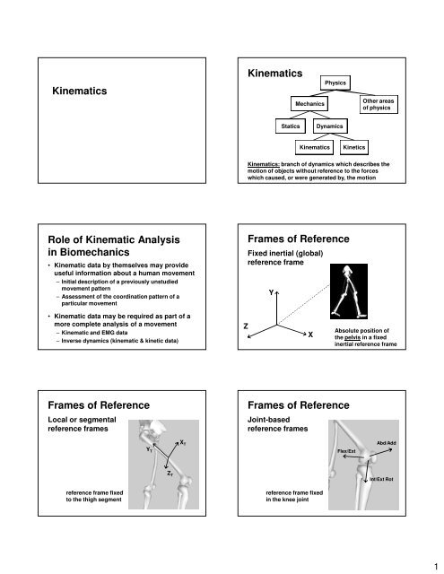
<strong><strong>K<strong>in</strong>ematic</strong>s</strong><strong><strong>K<strong>in</strong>ematic</strong>s</strong>MechanicsPhysicsOther areas<strong>of</strong> physicsStaticsDynamics<strong><strong>K<strong>in</strong>ematic</strong>s</strong>K<strong>in</strong>etics<strong><strong>K<strong>in</strong>ematic</strong>s</strong>: branch <strong>of</strong> dynamics which describes themotion <strong>of</strong> objects without reference to the forceswhich caused, or were generated by, the motion<strong>Role</strong> <strong>of</strong> <strong>K<strong>in</strong>ematic</strong> <strong>Analysis</strong><strong>in</strong> <strong>Biomechanics</strong>• <strong>K<strong>in</strong>ematic</strong> data by themselves may provideuseful <strong>in</strong>formation about a human movement– Initial description <strong>of</strong> a previously unstudiedmovement pattern– Assessment <strong>of</strong> the coord<strong>in</strong>ation pattern <strong>of</strong> aparticular movementFrames <strong>of</strong> ReferenceFixed <strong>in</strong>ertial (global)reference frameY• <strong>K<strong>in</strong>ematic</strong> data may be required as part <strong>of</strong> amore complete analysis <strong>of</strong> a movement– <strong>K<strong>in</strong>ematic</strong> and EMG data– Inverse dynamics (k<strong>in</strong>ematic & k<strong>in</strong>etic data)ZXAbsolute position <strong>of</strong>the pelvis <strong>in</strong> a fixed<strong>in</strong>ertial reference frameFrames <strong>of</strong> ReferenceFrames <strong>of</strong> ReferenceLocal or segmentalreference framesJo<strong>in</strong>t-basedreference framesX TAbd/AddY TFlex/ExtZ TInt/Ext Rotreference frame fixedto the thigh segmentreference frame fixed<strong>in</strong> the knee jo<strong>in</strong>t1
<strong>K<strong>in</strong>ematic</strong> variablesL<strong>in</strong>ear k<strong>in</strong>ematics <strong>of</strong> particles (po<strong>in</strong>ts)– Position - location at a given time– Displacement - change <strong>in</strong> position over aperiod <strong>of</strong> time (compare with distance)– Velocity - rate <strong>of</strong> change <strong>in</strong> position withrespect to time (compare with speed)– Acceleration - rate <strong>of</strong> change <strong>in</strong> velocity withrespect to time– Jerk - rate <strong>of</strong> change <strong>in</strong> acceleration withrespect to time*All are vector quantities(except distance and speed)Position & DisplacementDegrees <strong>of</strong> freedom - the m<strong>in</strong>imum number <strong>of</strong><strong>in</strong>dependent parameters necessary to specifythe configuration <strong>of</strong> a systemA po<strong>in</strong>t has 3 degrees<strong>of</strong> freedom, so itsposition is def<strong>in</strong>ed by 3coord<strong>in</strong>ates (x, y, and z)ZYXPosition & DisplacementIn two-dimensional analysis, only two quantitiesare needed to completely describe the position<strong>of</strong> a po<strong>in</strong>t or particleY5r3PXThe position <strong>of</strong> po<strong>in</strong>tP can be convenientlydenoted by a vector r,with r def<strong>in</strong>ed asr = 3 i + 5 ji and j are unit vectors<strong>in</strong> the directions <strong>of</strong> Xand Y, respectivelyPosition & DisplacementYr 1P 1P 2r 2XSay that the po<strong>in</strong>t movesfrom position 1 (P 1 ) toposition 2 (P 2 ) such thatr 1 = 3 i + 5 j andr 2 = 8 i + 7 jHow do we represent thedisplacement as a vector?Position & DisplacementYr 1d (r 1 -r 2 )P 1P 2r 2∆x∆yXThe displacement vector (d)is def<strong>in</strong>ed asd = r 2 - r 1 , sod = (8-3) i + (7-5) j = 5 i + 2 jThat is, the position haschanged 5 units <strong>in</strong> the Xdirection (∆x) and 2 units <strong>in</strong>the Y direction (∆y)VelocityYd (r 1 -r 2 )P 2P 1 ∆y∆xr 1r 2XVelocity is the rate at whichthe X and Y coord<strong>in</strong>ates arechang<strong>in</strong>gThe average velocity <strong>in</strong> theX direction is given by_v X = ∆x∆tand the <strong>in</strong>stantaneousvelocity <strong>in</strong> the X direction isgiven by.v X = lim ∆x = dx = x∆t→0 ∆t dt2
VelocityVelocityWhereas the position vectorto po<strong>in</strong>t P was given byYr 1d (r 1 -r 2 )P 2P 1 ∆y∆xr 2XThe average velocity <strong>in</strong> theY direction is given by_v Y = ∆y∆tand the <strong>in</strong>stantaneousvelocity <strong>in</strong> the Y direction isgiven by.v Y = lim ∆y = dy = y∆t→0 ∆t dtYr = x i + y jv 1the vector representation <strong>of</strong>v 2the velocity <strong>of</strong> po<strong>in</strong>t P isP 2written as. . .P 1 v = r = x i + y jXThe velocity vector v willalways be tangent to thepath followed by po<strong>in</strong>t PVelocityVelocityXtangent l<strong>in</strong>ex ix i-1x i+1When data are expressed<strong>in</strong> digital form, a true<strong>in</strong>stantaneous velocitycannot be calculatedIt can be approximated,however, us<strong>in</strong>g f<strong>in</strong>itedifference techniques.v X(i) = x ≈ x i+1 − x i-12∆tThe equation v X(i) = (x i+1 − x i-1 ) / 2∆tis a first order central difference equation, and can beapplied to all data po<strong>in</strong>ts except the first and lastTo estimate the velocity for the first po<strong>in</strong>t use a secondorder,forward difference equationv X(1) = -3x 1 + 4x 2 − x 32∆tand for the last po<strong>in</strong>t use a second-order, backwarddifference equation∆t∆ttAs ∆t gets smaller, theapproximation gets betterv X(n) = x n-2 − 4x n-1 + 3x n2∆tVelocityGiven the follow<strong>in</strong>g position data for the X coord<strong>in</strong>ate <strong>of</strong>a marker on the hip jo<strong>in</strong>t, calculate the velocityFrame Time (s) X coord (m) X vel (m/s)1 0.0000 1.73 ?2 0.0083 1.82 ?3 0.0167 1.88 ?4 0.0250 1.79 ?5 0.0333 1.83 ?First po<strong>in</strong>t, use forward differencev X(1) = (-3×1.73 + 4×1.82 − 1.88) / (2×0.0083) = 12.65VelocityGiven the follow<strong>in</strong>g position data for the X coord<strong>in</strong>ate <strong>of</strong>a marker on the hip jo<strong>in</strong>t, calculate the velocityFrame Time (s) X coord (m) X vel (m/s)1 0.0000 1.73 12.652 0.0083 1.82 ?3 0.0167 1.88 ?4 0.0250 1.84 ?5 0.0333 1.85 ?Po<strong>in</strong>ts 2 - 4, use central differencev X(2) = (1.88 − 1.73) / (2×0.0083) = 9.04v X(3) = (1.84 − 1.82) / (2×0.0083) = 1.20v X(4) = (1.85 − 1.88) / (2×0.0083) = -1.813
VelocityGiven the follow<strong>in</strong>g position data for the X coord<strong>in</strong>ate <strong>of</strong>a marker on the hip jo<strong>in</strong>t, calculate the velocityFrame Time (s) X coord (m) X vel (m/s)1 0.0000 1.73 12.652 0.0083 1.82 9.043 0.0167 1.88 1.204 0.0250 1.84 -1.815 0.0333 1.85 ?YAccelerationP 1P 2∆vThe vector change <strong>in</strong>velocity (∆v) is given by∆v = v 2 − v 1v 2v 1It can be represented <strong>in</strong>terms <strong>of</strong> the change <strong>of</strong>velocity <strong>in</strong> the X and YdirectionsLast po<strong>in</strong>t, use backward differencev 1 v 2∆v∆v Xv X(5) = (1.88 − 4×1.84 + 3×1.85) / (2×0.0083) = 4.22X∆v YAcceleration∆v XAcceleration∆v XYX∆v Yv 1 v 2the X direction is given by_a X = ∆v X∆vThe average acceleration <strong>in</strong>P 2∆tP 1and the <strong>in</strong>stantaneousacceleration <strong>in</strong> the Xdirection is given by.a X = lim ∆v X = dv X = v X∆t→0∆t dtYX∆v Yv 1 v 2the Y direction is given by_a Y = ∆v Y∆vThe average acceleration <strong>in</strong>P 2∆tP 1and the <strong>in</strong>stantaneousacceleration <strong>in</strong> the Ydirection is given by.a Y = lim ∆v Y = dv Y = v Y∆t→0∆t dtYAccelerationthe vector representation <strong>of</strong>v 1 P 2the acceleration <strong>of</strong> po<strong>in</strong>t Pa T(2)is written asP 1 . .. .. ..v 2a = v = r = x i + y ja N(2)XWhereas the velocity vector<strong>of</strong> po<strong>in</strong>t P was given by. . .v = r = x i + y jThe acceleration vector, a,will have two components,tangent to and normal tothe path followed by po<strong>in</strong>t PAccelerationA similar f<strong>in</strong>ite difference approach as for velocity can beused to estimate accelerationA first-order, central difference equation for acceleration,written <strong>in</strong> terms <strong>of</strong> position data, isa X(i) = x i+1 − 2x i + x i-1∆t 2The second-order, forward and backward differenceequations for the first and last po<strong>in</strong>ts area X(1) = 2x 1 − 5x 2 + 4x 3 − x 4 a X(n) = -x n-3 + 4x n-2 − 5x n-1 + 2x n∆t 2 ∆t 24
AccelerationGiven the follow<strong>in</strong>g position data for the X coord<strong>in</strong>ate <strong>of</strong>a marker on the hip jo<strong>in</strong>t, calculate the velocityFrame Time (s) X coord (m) X vel (m/s) X accel (m/s 2 )1 0.0000 1.73 12.65 ?2 0.0083 1.82 9.04 ?3 0.0167 1.88 1.20 ?4 0.0250 1.79 -1.81 ?5 0.0333 1.83 4.22 ?AccelerationGiven the follow<strong>in</strong>g position data for the X coord<strong>in</strong>ate <strong>of</strong>a marker on the hip jo<strong>in</strong>t, calculate the velocityFrame Time (s) X coord (m) X vel (m/s) X accel (m/s 2 )1 0.0000 1.73 12.65 1306.42 0.0083 1.82 9.04 ?3 0.0167 1.88 1.20 ?4 0.0250 1.79 -1.81 ?5 0.0333 1.83 4.22 ?First po<strong>in</strong>t, use forward differencea X(1) = (2×1.73 − 5×1.82 + 4×1.88 − 1.79) / (0.0083) 2 = 1306.4Po<strong>in</strong>ts 2 - 4, use central differencea X(2) = (1.88 − 2×1.82 + 1.73) / (0.0083) 2 = -435.5a X(3) = (1.84 − 2×1.88 + 1.82) / (0.0083) 2 = -1451.6a X(4) = (1.85 − 2×1.84 + 1.88) / (0.0083) 2 = 725.8AccelerationGiven the follow<strong>in</strong>g position data for the X coord<strong>in</strong>ate <strong>of</strong>a marker on the hip jo<strong>in</strong>t, calculate the velocityFrame Time (s) X coord (m) X vel (m/s) X accel (m/s 2 )1 0.0000 1.73 12.65 1306.42 0.0083 1.82 9.04 -435.53 0.0167 1.88 1.20 -1451.64 0.0250 1.79 -1.81 725.85 0.0333 1.83 4.22 ?Last po<strong>in</strong>t, use backward differencea X(5) = (-1.82 + 4×1.88 − 5×1.84 + 2×1.85) / (0.0083) 2 = 2903.2Velocity & AccelerationNote that if global polynomials or spl<strong>in</strong>efunction were used to fit and/or smooth thedata, then velocity and acceleration can bedeterm<strong>in</strong>ed analyticallyExample:x(t) = 3 + 7t − 4t 2 + 8t 3 + 5t 4 − 2t 5.v(t) = dx = x = 7 − 8t + 24t 2 + 20t 3 − 10t 4dt.a(t) = dv = v = -8 + 48t +60t 2 − 40t 3dtBack to Smooth<strong>in</strong>gWhy were we so careful to properly smooth outhigh frequency noise from our data?Smooth<strong>in</strong>g & DifferentiationDifferentiation amplifies high-frequency noise5
Smooth<strong>in</strong>g & Differentiation• For the 1 st derivative (velocity) signalamplitude <strong>in</strong>creases proportional t<strong>of</strong>requency• For the 2 nd derivative (acceleration) signalamplitude <strong>in</strong>creases proportional t<strong>of</strong>requency squared• This is why it is so important to elim<strong>in</strong>atesources <strong>of</strong> high frequency noise before datacollection, and suppress the rema<strong>in</strong><strong>in</strong>g highfrequency noise through low-pass filter<strong>in</strong>gAngular <strong>K<strong>in</strong>ematic</strong> VariablesThe follow<strong>in</strong>g is applicable to rigid bodies <strong>in</strong>planar motion (3-D is more complicated)– Angular Position - angle at a given time– Angular Displacement - change <strong>in</strong> angularposition over a period <strong>of</strong> time– Angular Velocity - rate <strong>of</strong> change <strong>in</strong> angularposition with respect to time– Angular Acceleration - rate <strong>of</strong> change <strong>in</strong>angular velocity with respect to timeAngular Position (Orientation)Degrees <strong>of</strong> freedom - a rigid body <strong>in</strong> 3-D spacerequires six quantities to completely describe itsposition and orientationAngular Position (Orientation)In two-dimensional analysis, only two l<strong>in</strong>earcoord<strong>in</strong>ates (x, y) and one angle (θ) are neededto completely describe the position andorientation <strong>of</strong> a rigid bodyCould use the x, y, andz coord<strong>in</strong>ate <strong>of</strong> thecenter <strong>of</strong> mass, plusthe angular rotationsrelative to the globalreference frame(other coord<strong>in</strong>ate setsare also possible)(x,y,z)Yθ 2θ 3Zθ 1XY(x,y)θXSo <strong>in</strong> planar analyses,you must know the xand y coord<strong>in</strong>ates <strong>of</strong> atleast one po<strong>in</strong>t on eachbody, plus the anglerelative to some fixedreferenceAngular Position (Orientation)Segment angles, relative to the right horizontal,can be calculated us<strong>in</strong>g the coord<strong>in</strong>ates <strong>of</strong>markers at the ends <strong>of</strong> the segmentAngular Position (Orientation)Y(x 1 ,y 1 )The segment angle canbe calculated anywhere<strong>in</strong> the first two quadrantsus<strong>in</strong>g the law <strong>of</strong> cos<strong>in</strong>es:Y(x 1 ,y 1 )First, create a third,imag<strong>in</strong>ary po<strong>in</strong>t, to theright along the x-axisθ(x 2 ,y 2 )a 2 = b 2 + c 2 − 2bc × cos θ( )θ = cos -1 b 2 + c 2 − a 22bcθ(x 2 ,y 2 )(x 3 ,y 3 )The value <strong>of</strong> y 3 is thesame as y 2 , the value <strong>of</strong>x 3 simply needs to belarger than x 2XX6
Angular Position (Orientation)Angular Position (Orientation)Y(x 1 ,y 1 )b(x 2 ,y 2 )aθc(x 3 ,y 3 )XLabel the sides a, b, andc as shown, and solvethe equation for θθ = cos -1 b 2 + c 2 − a 2where( )2bca = √ (x 3 − x 1 ) 2 + (y 3 − y 1 ) 2b = √ (x 2 − x 1 ) 2 + (y 2 − y 1 ) 2c = √ (x 3 − x 2 ) 2 + (y 3 − y 2 ) 2Y(3,6)b(5,2)aθc(8,2)XWith po<strong>in</strong>t 1 (3,6), po<strong>in</strong>t2 (5,2), and po<strong>in</strong>t 3 (8,2)a = √ (8−3) 2 + (2−6) 2 = 6.4b = √ (5−3) 2 + (2−6) 2 = 4.5c = √ (8−5) 2 + (2−2) 2 = 3.0θ = cos -1 4.5 2 + 3.0 2 − 6.4 2θ = 115.7°( )2(4.5)(3.0)Angular Position (Orientation)Once segment angles are known, relative jo<strong>in</strong>tangles can be easily calculatedYθ THIGHθ SHANKXJo<strong>in</strong>t angles are typicallycalculated as the angle <strong>of</strong>the proximal segmentm<strong>in</strong>us the angle <strong>of</strong> thedistal segmentθ KNEE = θ THIGH − θ SHANKThis would make kneeangle 0 at full extension,pos for flexion, and negfor hyperextensionAngular <strong><strong>K<strong>in</strong>ematic</strong>s</strong>• For planar (2-D) motion, the relationshipsbetween angular displacement, angularvelocity, and angular acceleration areperfectly analogous to l<strong>in</strong>ear displacement,l<strong>in</strong>ear velocity, and l<strong>in</strong>ear acceleration• Once segment or jo<strong>in</strong>t angles are known,angular velocities and angular accelerationscan be calculated us<strong>in</strong>g the same f<strong>in</strong>itedifference approach as we used for l<strong>in</strong>earvelocity and l<strong>in</strong>ear accelerationAcknowledgementI want to acknowledge Brian Umberger, PhDfor the organization <strong>of</strong> much <strong>of</strong> the <strong>in</strong>formationpresented on these slides7