Further Exercises on the Euler-Lagrange Equation

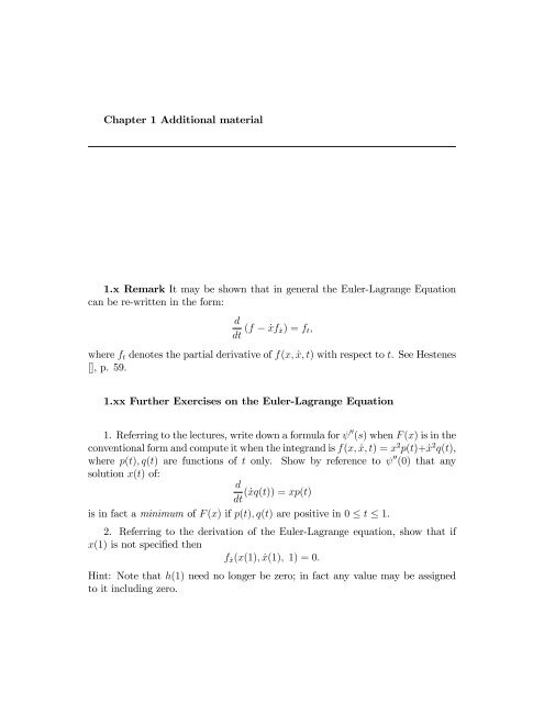
Chapter 1 Additional material1.x Remark It may be shown that in general the Euler-Lagrange Equationcan be re-written in the form:ddt (f _xf _x) = f t ;where f t denotes the partial derivative of f(x; _x; t) with respect to t. See Hestenes[], p. 59.1.xx <strong>Further</strong> <strong>Exercises</strong> on the Euler-Lagrange Equation1. Referring to the lectures, write down a formula for 00 (s) when F (x) is in theconventional form and compute it when the integrand is f(x; _x; t) = x 2 p(t)+ _x 2 q(t),where p(t); q(t) are functions of t only. Show by reference to 00 (0) that anysolution x(t) of:d( _xq(t)) = xp(t)dtis in fact a minimum of F (x) if p(t); q(t) are positive in 0 t 1.2. Referring to the derivation of the Euler-Lagrange equation, show that ifx(1) is not speci…ed thenf _x (x(1); _x(1); 1) = 0:Hint: Note that h(1) need no longer be zero; in fact any value may be assignedto it including zero.

3. Show that if x(0) and x(1) are not speci…ed then for = 0 and = 1 wehave:f _x (x(); _x(); ) = 0:Use these conditions to …nd the particular function x(t) which minimises theintegral:Z 10fx + _x + x _x + 1 2 _x2 g dtwhen the end-point values of x(t) are not speci…ed.4. Use the Lagrange Multiplier Method to solve:subject toand x(0) = x(1) = 0.min F (x) =Z 10Z 10x(t) 2 dt = 2_x(t) 2 dt5. Use the Lagrange Multiplier Method to solve:min F (x) =Z 10fx 2 + _x(t) 2 g dtsubject to Z 1x(t)e 2t dt = 10and x(0) = 1 and lim t!1 x(t) = 0. [Hint: Take the upper limit to be , solve,and then take to the limit. See also the poscript section below.]6. Maximise over x(t) the expression R =20sin t x(t) dt subject to:Z =20x(t) dt = 0;Z =20t x(t) dt = 0;Z =20x(t) 2 dt = 1:Comment: This problem may be treated geometrically; it asks for a vector xof length 1 (in the appropriate norm jj:jj 2 ) perpendicular to the vectors u; v: the

constant function function u 1 and the function v t and with maximalprojection onto the vector w sin t. A geometric tool is provided by the Gram-Schmidt process, from where it is clear that x(t) needs to be an appropriate linearcombination of u; v; w. The same conclusion is drawn from the Euler-Lagrangeequations, the appropriate scalars being Lagrange multipliers.7. Maximise the integral R +1x(t) log x(t) dt subject to:1Z +11x(t) dt = 1;Z +11t 2 x(t) dt = 2 :This is a problem similar to the last, but with connections with probability; it asksfor a probability distribution x(t) of a random variable t, with the …rst constraintbeing about its expectation and the second about its variance. [Hint: Refer tothe de…nition of the gamma function.]8. A country’s debt D t obeys the equation:D 0 t = rD t + M tS twhere r is the bank rate, M t is the rate at which raw materials are imported andS t is the rate at which goods are exported. In order to clear an initial debt ofD 0 by time T precisely the government proposes to maximize production over thetime range [0; T ] on the assumption that the output is always sold. Assuming aproduction function S t = a p M t with a > 0 and writing x t = M t S t = S 2 t =a 2 S tshow that the government’s problem amounts to maximising:subject toZ T0Z T0pa2 + 4x t dte rt x t dt = D 0 ;where it is assumed that x 0 = 0. Find the extremal curve for the problem andshow that the plan is feasible if and only if:D 0 = a2 (1 cosh rT ):2r

[Hint: Find S t in terms of x t and integrate the debt equation.]9. Maximise R 1f(t)p x(t) dt subject to R 1x(t) dt = c.010. Maximise R 10 f(t)x(t) dt subject to R 1x(t) dt = c where 1 .0011. For the problem:subject tominZ T0(x 2 + _x 2 ) dtx(0) = c; x(T ) = 0;the trajectory is known to be of the formshow thatx T (t) = Ae t + Be t ;lim A T = 0:T !1Show also that, pointwise lim T !1 x T (t) = ce t . Interpreting x T (t) = x T (T ) fort > T , verify that the limit is uniform.12. For the problem:min 1 2subject to x(0) = 1; x(1) = 0 andZ 10Z 10(x 2 + _x 2 ) dtxe 2t dt = 1show that the optimal curve is x = 9e t 8e 2t .13. For the problem:minZ 20f r 2 + 2 _r 2 g 1=2 d

where = (1 =r) 1 and is a constant, while _r here denotes dr=d, show thatthe Euler-Lagrange Equation reduces to the (Ricatti) equation:where u = 1=r.14. Solve the problem:minsubject to x(0) = 0; x(1) = 1.d 2 ud 2 + u = 3 2 u2 ;Z 10(t 2 + x 2 + _x 2 ) dt1.xxx Postscript: Dealing with in…nite horizon problemsRecall problem 5 in the last section; the trajectory is found to be of theform:x(t) = Ae t + Be t + Ce t + De t ;where > > 0 and 6= . The problem speci…ed x(0); _x(0) as given andrequired lim t!1 x(t) = 0 and lim t!1 _x(t) = 0. It is natural to set A = B = 0and continue with the problem. In this note we justify the procedure. It willbe clear that the method extends beyond just two exponentially growing terms.We take our terminal conditions in the form:x(T ) = _x(T ) = 0:This yields the following matrix equation of boundary conditions:23 2 3 2 31 1 1 1 A x(0)6 7 6 B74 e T e T e T e T 5 4 C 5 = 6 _x(0)74 0 5 :e T e T e T e T D 0By Cramer’s rule we obtain:A T = linear combinations of:(e( )T ; e (+)T ; 1);1( ) 2 e (+)T + :::

The numerator is obvious from the expansion by the …rst column; the criticalterm of the denominator comes from the bottom row, corner and adjacent termboth of which create the appropriate term by multiplication with the top rightsubdeterminant of size 2. It now follows thatSimilarly,lim A T = 0:T !1and againB T = linear combinations of:(e( )T ; e (+)T ; 1);1( ) 2 e (+)T + :::lim B T = 0:T !1We consider a similar problem in the <strong>Exercises</strong> (11?): Exercise:For theproblem:subject toZ T0minZ Tthe trajectory is known to be of the formshow that0(x 2 + _x 2 ) dtxe 2t dt = 1 and x(0) = 1; x(T ) = 0;x(t) = Ae t + Be t + Ce 2t ;lim A T = 0:T !1Solution: The two boundary conditions and the constraint equation lead to thematrix equation:21 1 14 e T e T e 2T1 e T 1(1 e 3T 1) 3 4 e 4T )3 25 4ABC325 = 410135 :

The matrix has determinant with dominant term e T 141= 1 3 12 eT , soA = A T = linear combinations of:(e T ; e 2T ; e T ; e 3T ; e 4T ; e 5T ; 1)112 eT + :::! 0:A similar calculation yieldsB T = e T ( 1 4! 3 12 = 9;41) linear combinations of:(e T ; e 2T ; e T ; e 3T ; e 4T ; e 5T ; 1)112 eT + :::but it is easier to set A = 0, now that that has beeen justi…ed, and to use theinitial condition and the constraint equation (to 1).