PSTricks pst-plot plotting data and functions - Welcome to ftp.eq.uc.pt.
PSTricks pst-plot plotting data and functions - Welcome to ftp.eq.uc.pt.
PSTricks pst-plot plotting data and functions - Welcome to ftp.eq.uc.pt.
- No tags were found...

Create successful ePaper yourself
Turn your PDF publications into a flip-book with our unique Google optimized e-Paper software.
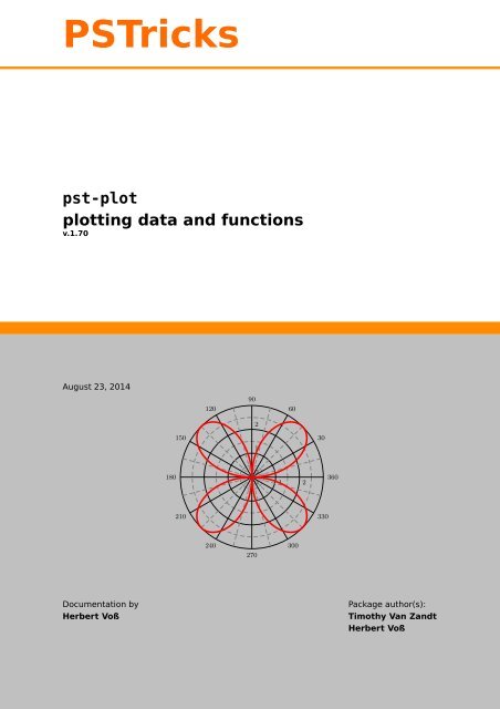
<strong>PSTricks</strong><strong>pst</strong>-<strong>plot</strong><strong>plot</strong>ting <strong>data</strong> <strong>and</strong> <strong>functions</strong>v.1.70August23,2014120902601501301800012360210330240270300DocumentationbyHerbert VoßPackage author(s):Timothy Van Z<strong>and</strong>tHerbert Voß
2This version of <strong>pst</strong>-<strong>plot</strong> uses the extended keyval h<strong>and</strong>ling of <strong>pst</strong>-xkey<strong>and</strong>hasalo<strong>to</strong>fthemacroswhichwererecentlyinthepackage<strong>pst</strong>ricks-add.This documentation describes only the new <strong>and</strong> changed stuff. For the defaultbehaviour look in<strong>to</strong> the documentation part of the base <strong>pst</strong>ricks package.Youfindthedocumentationhere: http://mirrors.ctan.org/graphics/<strong>pst</strong>ricks/base/doc/.Thanks <strong>to</strong>: Guillaume van Baalen; Stefano Baroni; Martin Chicoine; GerryCoombes; Ulrich Dirr; Chris<strong>to</strong>phe Fourey; Hubert Gäßlein; Jürgen Gilg; DenisGirou; Peter Hutnick; Chris<strong>to</strong>phe Jorssen; Uwe Kern; Alex<strong>and</strong>er Kornrumpf;Manuel Luque; Patrice Mégret; Jens-Uwe Morawski; Tobias Nähring;RolfNiepraschk;MartinPaech;AlanRis<strong>to</strong>w;ChristineRömer;ArnaudSchmittbuhl
Contents 3ContentsI. Basic comm<strong>and</strong>s, connections <strong>and</strong> labels 51. Introd<strong>uc</strong>tion 52. Plotting <strong>data</strong> records 53. Plotting mathematical <strong>functions</strong> 7II. New comm<strong>and</strong>s 84. Extended syntax 85. New Macro \psBox<strong>plot</strong> 106. The psgraph environment 156.1. Coordinates of the psgraph area . . . . . . . . . . . . . . . . . . . . . . . . 216.2. The new o<strong>pt</strong>ions for psgraph . . . . . . . . . . . . . . . . . . . . . . . . . . 216.3. The new macro \pslegend for psgraph . . . . . . . . . . . . . . . . . . . . 227. \psxTick <strong>and</strong> \psyTick 258. \<strong>pst</strong>ScalePoints 259. New or extended o<strong>pt</strong>ions 269.1. Introd<strong>uc</strong>tion . . . . . . . . . . . . . . . . . . . . . . . . . . . . . . . . . . . 269.2. O<strong>pt</strong>ion <strong>plot</strong>style (Chris<strong>to</strong>ph Bersch) . . . . . . . . . . . . . . . . . . . . . 299.3. O<strong>pt</strong>ion xLabels, yLabels, xLabelsrot, <strong>and</strong> yLabelsrot . . . . . . . . . . 299.4. O<strong>pt</strong>ion xLabelOffset <strong>and</strong> ylabelOffset . . . . . . . . . . . . . . . . . . . 309.5. O<strong>pt</strong>ion yMaxValue <strong>and</strong> yMinValue . . . . . . . . . . . . . . . . . . . . . . . 309.6. O<strong>pt</strong>ion axesstyle . . . . . . . . . . . . . . . . . . . . . . . . . . . . . . . . 329.7. O<strong>pt</strong>ion xyAxes, xAxis <strong>and</strong> yAxis . . . . . . . . . . . . . . . . . . . . . . . . 349.8. O<strong>pt</strong>ion labels . . . . . . . . . . . . . . . . . . . . . . . . . . . . . . . . . . 349.9. O<strong>pt</strong>ions xlabelPos <strong>and</strong> ylabelPos . . . . . . . . . . . . . . . . . . . . . . . 359.10. O<strong>pt</strong>ions x|ylabelFontSize <strong>and</strong> x|ymathLabel . . . . . . . . . . . . . . . . 369.11. O<strong>pt</strong>ions xlabelFac<strong>to</strong>r <strong>and</strong> ylabelFac<strong>to</strong>r . . . . . . . . . . . . . . . . . . 379.12. O<strong>pt</strong>ions decimalSepara<strong>to</strong>r <strong>and</strong> comma . . . . . . . . . . . . . . . . . . . . 389.13. O<strong>pt</strong>ions xyDecimals, xDecimals <strong>and</strong> yDecimals . . . . . . . . . . . . . . . 399.14. O<strong>pt</strong>ion triglabels . . . . . . . . . . . . . . . . . . . . . . . . . . . . . . . 409.15. O<strong>pt</strong>ion ticks . . . . . . . . . . . . . . . . . . . . . . . . . . . . . . . . . . . 479.16. O<strong>pt</strong>ion tickstyle . . . . . . . . . . . . . . . . . . . . . . . . . . . . . . . . 489.17. O<strong>pt</strong>ions ticksize, xticksize, yticksize . . . . . . . . . . . . . . . . . . 489.18. O<strong>pt</strong>ions subticks, xsubticks, <strong>and</strong> ysubticks . . . . . . . . . . . . . . . . 509.19. O<strong>pt</strong>ions subticksize, xsubticksize, ysubticksize . . . . . . . . . . . . 509.20. tickcolor <strong>and</strong> subtickcolor . . . . . . . . . . . . . . . . . . . . . . . . . 51
Contents 49.21. ticklinestyle <strong>and</strong> subticklinestyle . . . . . . . . . . . . . . . . . . . . 529.22. logLines . . . . . . . . . . . . . . . . . . . . . . . . . . . . . . . . . . . . . 529.23. xylogBase, xlogBase <strong>and</strong> ylogBase . . . . . . . . . . . . . . . . . . . . . . 549.24. xylogBase . . . . . . . . . . . . . . . . . . . . . . . . . . . . . . . . . . . . 549.25. ylogBase . . . . . . . . . . . . . . . . . . . . . . . . . . . . . . . . . . . . . 559.26. xlogBase . . . . . . . . . . . . . . . . . . . . . . . . . . . . . . . . . . . . . 579.27. No logstyle (xylogBase={}) . . . . . . . . . . . . . . . . . . . . . . . . . . . 589.28. O<strong>pt</strong>ion tickwidth <strong>and</strong> subtickwidth . . . . . . . . . . . . . . . . . . . . . 599.29. O<strong>pt</strong>ion psgrid, gridcoor, <strong>and</strong> gridpara . . . . . . . . . . . . . . . . . . . 6310.New o<strong>pt</strong>ions for \read<strong>data</strong> 6411.New o<strong>pt</strong>ions for \list<strong>plot</strong> 6511.1. O<strong>pt</strong>ions nStep, xStep, <strong>and</strong> yStep . . . . . . . . . . . . . . . . . . . . . . . 6511.2. O<strong>pt</strong>ions nStart <strong>and</strong> xStart . . . . . . . . . . . . . . . . . . . . . . . . . . . 6711.3. O<strong>pt</strong>ions nEnd <strong>and</strong> xEnd . . . . . . . . . . . . . . . . . . . . . . . . . . . . . 6811.4. O<strong>pt</strong>ions yStart <strong>and</strong> yEnd . . . . . . . . . . . . . . . . . . . . . . . . . . . . 6911.5. O<strong>pt</strong>ions <strong>plot</strong>No, <strong>plot</strong>NoX, <strong>and</strong> <strong>plot</strong>NoMax . . . . . . . . . . . . . . . . . . . 6911.6. O<strong>pt</strong>ion changeOrder . . . . . . . . . . . . . . . . . . . . . . . . . . . . . . . 7212.New <strong>plot</strong> styles 7312.1. Plot style colordot <strong>and</strong> o<strong>pt</strong>ion Hue . . . . . . . . . . . . . . . . . . . . . . 7312.2. Plot style bar <strong>and</strong> o<strong>pt</strong>ion barwidth . . . . . . . . . . . . . . . . . . . . . . 7412.3. Plot style ybar . . . . . . . . . . . . . . . . . . . . . . . . . . . . . . . . . . 7612.4. Plotstyle LSM . . . . . . . . . . . . . . . . . . . . . . . . . . . . . . . . . . . 7712.5. Plotstyles values <strong>and</strong> values* . . . . . . . . . . . . . . . . . . . . . . . . . 8012.6. Plotstyles xvalues <strong>and</strong> xvalues* . . . . . . . . . . . . . . . . . . . . . . . 8113.Polar <strong>plot</strong>s 8214.New macros 8514.1. \psCoordinates . . . . . . . . . . . . . . . . . . . . . . . . . . . . . . . . . 8514.2. \psFixpoint . . . . . . . . . . . . . . . . . . . . . . . . . . . . . . . . . . . 8614.3. \psNew<strong>to</strong>n . . . . . . . . . . . . . . . . . . . . . . . . . . . . . . . . . . . . 8714.4. \psVec<strong>to</strong>rfield . . . . . . . . . . . . . . . . . . . . . . . . . . . . . . . . . 8915.Internals 9016.List of all o<strong>pt</strong>ional arguments for <strong>pst</strong>-<strong>plot</strong> 91References 93
5Part I.Basic comm<strong>and</strong>s, connections <strong>and</strong>labels1. Introd<strong>uc</strong>tionThe <strong>plot</strong>ting comm<strong>and</strong>s described in this part are defined in the very first version of<strong>pst</strong>-<strong>plot</strong>.tex <strong>and</strong> available for all new <strong>and</strong> ancient versions.The \psdots, \psline, \pspolygon, \pscurve, \psecurve <strong>and</strong> \psccurve graphicsobjects let you <strong>plot</strong> <strong>data</strong> in a variety of ways. However, first you have <strong>to</strong> generate the<strong>data</strong> <strong>and</strong> enter it as coordinate pairs x,y. The <strong>plot</strong>ting macros in this section give youother ways <strong>to</strong> get <strong>and</strong> use the <strong>data</strong>.To parameter <strong>plot</strong>style=style determines what kind of <strong>plot</strong> you get. Valid stylesaredots,line,polygon, curve,ecurve,ccurve. E,g.,ifthe<strong>plot</strong>style ispolygon, thenthe macro becomes a variant of the \pspolygon object.You can use arrows with the <strong>plot</strong> styles that are open curves, but there is no o<strong>pt</strong>ionalargument for specifying the arrows. You have <strong>to</strong> use the arrows parameter instead.No PostScri<strong>pt</strong> error checking is provided for the <strong>data</strong> arguments. There are systemdependentlimits on the amount of <strong>data</strong> T E X <strong>and</strong> PostScri<strong>pt</strong> can h<strong>and</strong>le. You are m<strong>uc</strong>hless likely <strong>to</strong> exceed the PostScri<strong>pt</strong> limits when you use the line, polygon or dots <strong>plot</strong>style, with showpoints=false, linearc=0<strong>pt</strong>, <strong>and</strong> no arrows.Note that the lists of <strong>data</strong> generated or used by the <strong>plot</strong> comm<strong>and</strong>s cannot containunits. The values of \psxunit <strong>and</strong> \psyunit are used as the unit.2. Plotting <strong>data</strong> records\file<strong>plot</strong> [O<strong>pt</strong>ions] {file}\psfile<strong>plot</strong> [O<strong>pt</strong>ions] {file}\<strong>data</strong><strong>plot</strong> [O<strong>pt</strong>ions] {\〈macro〉}\ps<strong>data</strong><strong>plot</strong> [O<strong>pt</strong>ions] {\〈macro〉}\save<strong>data</strong>{\〈macro〉}[<strong>data</strong>]\read<strong>data</strong>{\〈macro〉}{file}\psreadColumnData{colNo}{delimiter}{\〈macro〉}{filename}\list<strong>plot</strong>{<strong>data</strong>}\pslist<strong>plot</strong>{<strong>data</strong>}The macros with a preceeding ps are <strong>eq</strong>uivalent <strong>to</strong> those without.\file<strong>plot</strong> is the simplest of the <strong>plot</strong>ting <strong>functions</strong> <strong>to</strong> use. You just need a file thatcontainsalis<strong>to</strong>fcoordinates(withoutunits),s<strong>uc</strong>hasgeneratedbyMathematicaorothermathematical packages. The <strong>data</strong> can be delimited by curly braces { }, parentheses( ), commas,<strong>and</strong>/or white space. Bracketing all the <strong>data</strong> with square brackets [ ] willsignificantlyspeedu<strong>pt</strong>herateatwhichthe<strong>data</strong>isread,buttherearesystem-dependent
2. Plotting <strong>data</strong> records 6limits on how m<strong>uc</strong>h <strong>data</strong> T E X can read like this in one chunk. (The [ must go at thebeginning of a line.) The file should not contain anything else (not even \endinput),exce<strong>pt</strong> for comments marked with %.\file<strong>plot</strong> only recognizes the line, polygon <strong>and</strong> dots <strong>plot</strong> styles, <strong>and</strong> it ignoresthe arrows, linearc <strong>and</strong> showpoints parameters. The \list<strong>plot</strong> comm<strong>and</strong>, describedbelow, can also <strong>plot</strong> <strong>data</strong> from file, without these restrictions <strong>and</strong> with faster T E X processing.However, you are less likely <strong>to</strong> exceed PostScri<strong>pt</strong>’s memory or oper<strong>and</strong> stacklimits with \file<strong>plot</strong>.IfyoufindthatittakesT E Xalongtime<strong>to</strong>process your\file<strong>plot</strong> comm<strong>and</strong>,youmaywant <strong>to</strong> use the \PST<strong>to</strong>EPS comm<strong>and</strong> described on page ??. This will also red<strong>uc</strong>e T E X’smemory r<strong>eq</strong>uirements.\<strong>data</strong><strong>plot</strong> is also for <strong>plot</strong>ting lists of <strong>data</strong> generated by other programs, but you firsthave <strong>to</strong> retrieve the <strong>data</strong> with one of the following comm<strong>and</strong>s: <strong>data</strong> or the <strong>data</strong> in fileshouldconform<strong>to</strong>therulesdescribed aboveforthe<strong>data</strong>in\file<strong>plot</strong> (with\save<strong>data</strong>,the <strong>data</strong> must be delimited by [ ], <strong>and</strong> with \read<strong>data</strong>, bracketing the <strong>data</strong> with [ ]speeds things up). You can concatenate <strong>and</strong> reuse lists, as in\read<strong>data</strong>{\foo}{foo.<strong>data</strong>}\read<strong>data</strong>{\bar}{bar.<strong>data</strong>}\<strong>data</strong><strong>plot</strong>{\foo\bar}\<strong>data</strong><strong>plot</strong>[origin={0,1}]{\bar}The \read<strong>data</strong> <strong>and</strong> \<strong>data</strong><strong>plot</strong> combination is faster than \file<strong>plot</strong> if you reuse the<strong>data</strong>. \file<strong>plot</strong> uses less of T E X’s memory than \read<strong>data</strong> <strong>and</strong> \<strong>data</strong><strong>plot</strong> if you arealso use \PST<strong>to</strong>EPS.Here is a <strong>plot</strong> of ∫ sin(x)dx. The <strong>data</strong> was generated by Mathematica, withTable[{x,N[SinIntegral[x]]},{x,0,20}]<strong>and</strong> then copied <strong>to</strong> this document. \pspicture(4,3) \psset{xunit=.2cm,yunit=1.5cm}\save<strong>data</strong>{\my<strong>data</strong>}[{{0, 0}, {1., 0.946083}, {2., 1.60541}, {3., 1.84865}, {4., 1.7582},{5., 1.54993}, {6., 1.42469}, {7., 1.4546}, {8., 1.57419},{9., 1.66504}, {10., 1.65835}, {11., 1.57831}, {12., 1.50497},{13., 1.49936}, {14., 1.55621}, {15., 1.61819}, {16., 1.6313},{17., 1.59014}, {18., 1.53661}, {19., 1.51863}, {20., 1.54824}}]\<strong>data</strong><strong>plot</strong>[<strong>plot</strong>style=curve,showpoints,dotstyle=triangle]{\my<strong>data</strong>}\psline{}(0,2)(0,0)(22,0)\endpspicture\list<strong>plot</strong> is yet another way of <strong>plot</strong>ting lists of <strong>data</strong>. This time, should be alist of <strong>data</strong> (coordinate pairs), delimited only by white space. list is first exp<strong>and</strong>ed by
•••••••••3. Plotting mathematical<strong>functions</strong> 7T E X <strong>and</strong> then by PostScri<strong>pt</strong>. This means that list might be a PostScri<strong>pt</strong> program thatleaves on the stack a list of <strong>data</strong>, but you can also include <strong>data</strong> that has been retrievedwith \read<strong>data</strong> <strong>and</strong> \<strong>data</strong><strong>plot</strong>. However, when using the line, polygon or dots <strong>plot</strong>styleswith showpoints=false, linearc=0<strong>pt</strong> <strong>and</strong> no arrows, \<strong>data</strong><strong>plot</strong> is m<strong>uc</strong>h lesslikely than \list<strong>plot</strong> <strong>to</strong> exceed PostScri<strong>pt</strong>’s memory or stack limits. In the precedingexample, these restrictionswere notsatisfied,<strong>and</strong>sotheexampleis<strong>eq</strong>uivalent <strong>to</strong>when\list<strong>plot</strong> is used:...\list<strong>plot</strong>[<strong>plot</strong>style=curve,showpoints=true,dotstyle=triangle]{\my<strong>data</strong>}...3. Plotting mathematical <strong>functions</strong>\ps<strong>plot</strong> [O<strong>pt</strong>ions] {x ! min@}{x ! max@}{function}\parametric<strong>plot</strong> [O<strong>pt</strong>ions] {t ! min@}{t ! max@}{x(t) y(t)}\ps<strong>plot</strong> can be used <strong>to</strong> <strong>plot</strong> a function f(x), if you know a little PostScri<strong>pt</strong>. <strong>functions</strong>hould be the PostScri<strong>pt</strong> or algebraic code for calculating f(x). Note that you must usex as the dependent variable.\ps<strong>plot</strong>[<strong>plot</strong>points=200]{0}{720}{x sin}<strong>plot</strong>s sin(x) from 0 <strong>to</strong> 720 degrees, by calculating sin(x) roughly every 3.6 degrees <strong>and</strong>thenconnectingthepointswith\psline. Hereare<strong>plot</strong>sofsin(x)cos((x/2) 2 )<strong>and</strong>sin 2 (x):\pspicture(0,-1)(4,1)\psset{xunit=1.2<strong>pt</strong>}\ps<strong>plot</strong>[linecolor=gray,linewidth=1.5<strong>pt</strong>,<strong>plot</strong>style=curve]{0}{90}{x sin dup mul}\ps<strong>plot</strong>[<strong>plot</strong>points=100]{0}{90}{x sin x 2 div 2 exp cos mul}\psline{}(0,-1)(0,1) \psline{->}(100,0)\endpspicture\parametric<strong>plot</strong> is for a parametric <strong>plot</strong> of (x(t),y(t)). function is the PostScri<strong>pt</strong>code or algebraic expression for calculating the pair x(t) y(t).For example,• • • •\pspicture(3,3)\parametric<strong>plot</strong>[<strong>plot</strong>style=dots,<strong>plot</strong>points=13]%{-6}{6}{1.2 t exp 1.2 t neg exp}\endpspicture
8<strong>plot</strong>s 13 points from the hyperbola xy = 1, starting with (1.2 −6 ,1.2 6 ) <strong>and</strong> ending with(1.2 6 ,1.2 −6 ).Here is a parametric <strong>plot</strong> of (sin(t),sin(2t)):\pspicture(-2,-1)(2,1)\psset{xunit=1.7cm}\parametric<strong>plot</strong>[linewidth=1.2<strong>pt</strong>,<strong>plot</strong>style=ccurve]%{0}{360}{t sin t 2 mul sin}\psline{}(0,-1.2)(0,1.2)\psline{}(-1.2,0)(1.2,0)\endpspictureThe number of points that the \ps<strong>plot</strong> <strong>and</strong> \parametric<strong>plot</strong> comm<strong>and</strong>s calculateis set by the <strong>plot</strong>points= parameter. Using "curve" or its variants instead of"line" <strong>and</strong> increasing the value of <strong>plot</strong>points are two ways <strong>to</strong> get a smoother curve.Both ways increase the imaging time. Which is better depends on the complexity ofthe computation. (Note that all PostScri<strong>pt</strong> lines are ultimately rendered as a series(perhaps short) line segments.) Mathematica generally uses "line<strong>to</strong>" <strong>to</strong> connect thepointsinits<strong>plot</strong>s. Thedefaultminimumnumberof<strong>plot</strong>pointsforMathematicais25,butunlike \ps<strong>plot</strong> <strong>and</strong> \parametric<strong>plot</strong>, Mathematica increases the sampling fr<strong>eq</strong>uencyon sections of the curve with greater fl<strong>uc</strong>tuation.Part II.New comm<strong>and</strong>s4. Extended syntax for \ps<strong>plot</strong>, \psparametric<strong>plot</strong>, <strong>and</strong>\psaxesThere is now a new o<strong>pt</strong>ional argument for \ps<strong>plot</strong> <strong>and</strong> \psparametric<strong>plot</strong> <strong>to</strong> passadditionalPostScri<strong>pt</strong>comm<strong>and</strong>s in<strong>to</strong>thecode. Thismakestheuseof\<strong>pst</strong>Verb inmostcases superfluous.\ps<strong>plot</strong> [O<strong>pt</strong>ions] {x0}{x1} [PS comm<strong>and</strong>s] {function}\psparametric<strong>plot</strong> [O<strong>pt</strong>ions] {t0}{t1} [PS comm<strong>and</strong>s] {x(t) y(t)}\psaxes [O<strong>pt</strong>ions] {arrows} (x 0 ,y 0 )(x 1 ,y 1 )(x 2 ,y 2 )[Xlabel,Xangle] [Ylabel,Yangle]The macro \psaxes has now four o<strong>pt</strong>ional arguments, one for the setting, one for thearrows, one for the x-label <strong>and</strong> one for the y-label. If you want only a y-label, then leavethe x one em<strong>pt</strong>y. A missing y-label is possible. The following examples show how it canbe used.\begin{pspicture}(-1,-0.5)(12,5)\psaxes[Dx=100,dx=1,Dy=0.00075,dy=1]{->}(0,0)(12,5)[$x$,-90][$y$,180]\ps<strong>plot</strong>[linecolor=red, <strong>plot</strong>style=curve,linewidth=2<strong>pt</strong>,<strong>plot</strong>points=200]{0}{11}%[ /const1 3.3 10 8 neg exp mul def
4. Extended syntax 9/s 10 def/const2 6.04 10 6 neg exp mul def ] % o<strong>pt</strong>ional PS comm<strong>and</strong>s{ const1 x 100 mul dup mul mul Euler const2 neg x 100 mul dup mul mul expmul 2000 mul}\end{pspicture}y0.003000.002250.001500.0007500 100 200 300 400 500 600 700 800 900 1000 1100x
•5. NewMacro \psBox<strong>plot</strong> 105. New Macro \psBox<strong>plot</strong>A box-<strong>and</strong>-whisker <strong>plot</strong> (often called simply a box <strong>plot</strong>) is a his<strong>to</strong>gram-like method ofdisplaying <strong>data</strong>, invented by John.Tukey. The box-<strong>and</strong>-whisker <strong>plot</strong> is a box with endsat the quartiles Q 1 <strong>and</strong> Q 3 <strong>and</strong> has a statistical median M as a horizontal line in thebox. The "‘whiskers"* are lines <strong>to</strong> the farthest points that are not outliers (i.e., that arewithin 3/2 times the interquartile range of Q 1 <strong>and</strong> Q 3 ). Then, for every point more than3/2 times the interquartile range from the end of a box, is a dot.The only special o<strong>pt</strong>ional arguments, beside all other which are valid for drawinglines <strong>and</strong> filling areas, are IQLfac<strong>to</strong>r, barwidth, <strong>and</strong> arrowlength, where the latter isa fac<strong>to</strong>r which is multiplied with the barwidth for the line ends. The IQLfac<strong>to</strong>r, preset<strong>to</strong> 1.5, defines the area for the outliners. Theoutliners are <strong>plot</strong>ted as adot <strong>and</strong> takethesettings for s<strong>uc</strong>h a dot in<strong>to</strong> account, eg. dotstyle, dotsize, dotscale, <strong>and</strong> fillcolor.The default is the black dot.13012011010020012008908070602001 200850403020200120081000 1 2 3 4 5 6 7 8 9 10 11 12\begin{pspicture}(-1,-1)(12,14)
5. NewMacro \psBox<strong>plot</strong> 11\psset{yunit=0.1,fillstyle=solid}\save<strong>data</strong>{\<strong>data</strong>}[100 90 120 115 120 110 100 110 100 90 100 100 120 120 120]\rput(1,0){\psBox<strong>plot</strong>[fillcolor=red!30]{\<strong>data</strong>}}\rput(1,105){2001}\save<strong>data</strong>{\<strong>data</strong>}[90 120 115 116 115 110 90 130 120 120 120 85 100 130 130]\rput(3,0){\psBox<strong>plot</strong>[arrowlength=0.5,fillcolor=blue!30]{\<strong>data</strong>}}\rput(3,107){2008}\save<strong>data</strong>{\<strong>data</strong>}[35 70 90 60 100 60 60 80 80 60 50 55 90 70 70]\rput(5,0){\psBox<strong>plot</strong>[barwidth=40<strong>pt</strong>,arrowlength=1.2,fillcolor=red!30]{\<strong>data</strong>}}\rput(5,65){2001}\save<strong>data</strong>{\<strong>data</strong>}[60 65 60 75 75 60 50 90 95 60 65 45 45 60 90]\rput(7,0){\psBox<strong>plot</strong>[barwidth=40<strong>pt</strong>,fillcolor=blue!30]{\<strong>data</strong>}}\rput(7,65){2008}\save<strong>data</strong>{\<strong>data</strong>}[20 20 25 20 15 20 20 25 30 20 20 20 30 30 30]\rput(9,0){\psBox<strong>plot</strong>[fillcolor=red!30]{\<strong>data</strong>}}\rput(9,22){2001}\save<strong>data</strong>{\<strong>data</strong>}[20 30 20 35 35 20 20 60 50 20 35 15 30 20 40]\rput(11,0){\psBox<strong>plot</strong>[fillcolor=blue!30,linestyle=dashed]{\<strong>data</strong>}}\rput(11,25){2008}\psaxes[dy=1cm,Dy=10](0,0)(12,130)\end{pspicture}The next example uses an external file for the <strong>data</strong>, which must first be read by themacro\read<strong>data</strong>. Thenex<strong>to</strong>necreatesahorizontalbox<strong>plot</strong> byrotatingtheoutputwith−90 degrees.322824201612824100 1 200 4 8 12 16 20 24 28 32\read<strong>data</strong>{\<strong>data</strong>}{box<strong>plot</strong>.<strong>data</strong>}
•5. NewMacro \psBox<strong>plot</strong> 12\begin{pspicture}(-1,-1)(2,10)\psset{yunit=0.25,fillstyle=solid}\save<strong>data</strong>{\<strong>data</strong>}[2 4 6 8 10 12 14 16 18 20 22 24 26 28 30 32]\rput(1,0){\psBox<strong>plot</strong>[fillcolor=blue!30]{\<strong>data</strong>}}\psaxes[dy=1cm,Dy=4](0,0)(2,35)\end{pspicture}%\begin{pspicture}(-1,-1)(11,2)\psset{xunit=0.25,fillstyle=solid}\save<strong>data</strong>{\<strong>data</strong>}[2 4 6 8 10 12 14 16 18 20 22 24 26 28 30 32]\rput{-90}(0,1){\psBox<strong>plot</strong>[yunit=0.25,fillcolor=blue!30]{\<strong>data</strong>}}\psaxes[dx=1cm,Dx=4](0,0)(35,2)\end{pspicture}It is also possible <strong>to</strong> read a <strong>data</strong> column from an external file:1008060402000 1 2 3 4\begin{filecontents*}{Data.dat}98, 3220, 1179, 2614, 923, 2221, 1058, 2513, 819, 553, 2941, 3711, 283, 2571, 5110, 789, 1710, 6, 41, 75
••••••••••••••••••••••••••••••5. NewMacro \psBox<strong>plot</strong> 13\end{filecontents*}\begin{pspicture}(-1,-1)(5,6)\psaxes[axesstyle=frame,dy=1cm,Dy=20,ticksize=4<strong>pt</strong> 0](0,0)(4,5)\psreadDataColumn{1}{,}{\<strong>data</strong>}{Data.dat}\rput(1,0){\psBox<strong>plot</strong>[fillcolor=red!40,yunit=0.05]{\<strong>data</strong>}}\psreadDataColumn{2}{,}{\<strong>data</strong>}{Data.dat}\rput(3,0){\psBox<strong>plot</strong>[fillcolor=blue!40,yunit=0.05]{\<strong>data</strong>}}\end{pspicture}With the o<strong>pt</strong>ional argument postAction one can modify the y value of the box<strong>plot</strong>,e.g. for an output with a vertical axis in logarithm scaling:10 4 0 1 2 3 4 5 6 7 810 310 210 110 010 −110 −2\begin{pspicture}(-1,-3)(9,5)\psset{fillstyle=solid}\psaxes[ylogBase=10,Oy=-2,logLines=y,ticksize=0 4<strong>pt</strong>, subticks=5](1,-2)(9,4)\rput(3,0){\psBox<strong>plot</strong>[fillcolor=red!30,barwidth=0.9cm,postAction=Log]{0.09 0.44 0.12 0.06 0.32 0.23 0.44 0.02 0.15 0.18 0 0.29 0 0.11 0.26 0.110 0.45 0.04 0.14 0.03 0.12 0.14 0.31 0.06 0.06 0.11 0.12 0.12 0.12 0.130.01 0.40 0.01 0.03 0.17 0 0.10 0.15 0.16 0.06 0.10 0.01 0.60 0.26 0.110.15 0.22 0.14 0.01 }}\rput(4,0){\psBox<strong>plot</strong>[fillcolor=red!30,barwidth=0.9cm,postAction=Log]{0.07 0.49 0.34 0.20 0.02 1.08 6.83 0.31 0.54 0.02 0.29 0.18 0.60 0.09 0.611.37 0.26 0.03 2.30 0.09 3.15 0.13 0.29 0.27 1.30 0.73 0.63 0.24 10.03 00.26 0.18 3.29 2.43 1.94 0.22 0.23 0.60 1.69 0.35 3.96 0.56 9.90 0.10 0.430.22 0.26 0.31 0.29 0.79 }}\rput(5,0){\psBox<strong>plot</strong>[fillcolor=red!30,barwidth=0.9cm,postAction=Log]{12.70 1.34 0.68 0.51 1.77 0.04 3.79 287.05 1.35 5.41 15.56 3.13 0.91 7.482.40 1.04 3.53 0.58 31.71 7.89 4.90 2.61 0.89 0.03 3.78 8.11 4.82 1.02 5.578.85 0.15 17.59 0.21 8.10 2.15 3.43 6.44 1.65 6.83 23.54 0.52 1.47 0.753.54 3.59 5.56 0.33 8.58 1.90 0.78 }}\rput(6,0){\psBox<strong>plot</strong>[fillcolor=red!30,barwidth=0.9cm,postAction=Log]{55.72 14.91 14.95 6.01 6.53 88.30 281.50 40.15 13.41 0.91 1.65 44.32 13.417.33 3.51 3.44 70.40 0.75 58.20 54.88 26.45 33.76 0.70 0.05 0.29 57.12
5. NewMacro \psBox<strong>plot</strong> 1414.30 31.11 18.56 0.48 21.33 1.15 2.22 3.88 1.78 151.25 7.77 137.92 0.503.01 1.99 23.18 119.59 17.50 15.87 13.63 21.85 23.53 68.72 2.90 }}\rput(7,0){\psBox<strong>plot</strong>[fillcolor=red!30,barwidth=0.9cm,postAction=Log]{1.19 1.94 13.40 7.40 267.30 5.94 11.05 6.51 2.94 5.45 5.24 231 4.48 0.68311.29 77.47 621.20 139.08 1933.59 2.52 100.96 11.02 153.43 26.67 83.844.31 106.34 15.90 1118.59 9.49 131.48 48.92 5.85 3.74 1.05 32.03 5.6945.10 12.43 238.56 28.75 1.01 119.29 12.09 31.18 16.60 29.67 138.5517.42 0.83 }}\rput(8,0){\psBox<strong>plot</strong>[fillcolor=red!30,barwidth=0.9cm,postAction=Log]{2077.45 762.10 469 143.60 685 3600 20.20 249.60 269 0.30 0.20 779.40 1.80146.80 1.30 32.50 137 2016.40 2.30 33.90 801.60 2.20 646.90 3600 1184 627500.50 238.30 477.40 3600 17.80 1726.80 2 316.70 174.50 2802.70 335.30201.20 1.10 247.10 2705.10 156.90 5.10 2342.50 3600 3600 72.70 47.40301.20 1.60 }}\end{pspicture}It uses the PostScri<strong>pt</strong> function Log instead of log. The latter cannot h<strong>and</strong>le zerovalues. The next examples shows how a very small intervall can be h<strong>and</strong>led:0.99400.99350.99300 1\psset{yunit=0.5cm}\begin{pspicture}(-2,-1)(2,11)\save<strong>data</strong>{\<strong>data</strong>}[0.9936 0.9937 0.9934 0.9936 0.9937 0.9938 0.9934 0.9933 0.99300.9935]\psaxes[Oy=0.9930,Dy=0.0005,dy=2cm](0,0)(1,10)\rput(.5,0){\psBox<strong>plot</strong>[barwidth=.5\psxunit,postAction=0.993 sub 1e4 mul]{\<strong>data</strong>}}\end{pspicture}
••••6. Thepsgraph environment 156. The psgraph environmentThis new environment psgraph does the scaling, it expects as parameter the values(without units!) for the coordinate system <strong>and</strong> the values of the physical width <strong>and</strong>height (with units!). The syntax is:\psgraph [O<strong>pt</strong>ions] {}%...(xOrig,yOrig)(xMin,yMin)(xMax,yMax){xLength}{yLength}\endpsgraph\begin{psgraph} [O<strong>pt</strong>ions] {}%...(xOrig,yOrig)(xMin,yMin)(xMax,yMax){xLength}{yLength}\end{psgraph}where the o<strong>pt</strong>ions are valid only for the the \psaxes macro. The first two argumentshave the usual <strong>PSTricks</strong> behaviour.• if (xOrig,yOrig) is missing, it is substituted <strong>to</strong> (xMin,xMax);• if(xOrig,yOrig)<strong>and</strong>(xMin,yMin)aremissing,theyarebothsubstituted<strong>to</strong>(0,0).The y-length maybe given as !; then the macro uses the same unit as for the x-axis.y6·10 85·10 84·10 83·10 82·10 81·10 87·10 8 0 5 10 15 20 25 x• • • • • • • • • • • • • •• • •• • •0·10 8\read<strong>data</strong>{\<strong>data</strong>}{demo1.<strong>data</strong>}\<strong>pst</strong>ScalePoints(1,1e-08){}{}% (x,y){additional x opera<strong>to</strong>r}{y op}\psset{llx=-1cm,lly=-1cm}\begin{psgraph}[axesstyle=frame,xticksize=0 7.59,yticksize=0 25,%subticks=0,ylabelFac<strong>to</strong>r=\cdot 10^8,Dx=5,dy=1\psyunit,Dy=1](0,0)(25,7.5){10cm}{6cm} % parameters\list<strong>plot</strong>[linecolor=red,linewidth=2<strong>pt</strong>,showpoints=true]{\<strong>data</strong>}\end{psgraph}In the following example, the y unit gets the same value as the one for the x-axis.
••••6. Thepsgraph environment 163y210x0 1 2 3 4 5\psset{llx=-1cm,lly=-0.5cm,ury=0.5cm}\begin{psgraph}(0,0)(5,3){6cm}{!} % x-y-axis with same unit\ps<strong>plot</strong>[linecolor=red,linewidth=1<strong>pt</strong>]{0}{5}{x dup mul 10 div}\end{psgraph}7·10 8 0 5 10 15 20 256·10 85·10 8y-Axis4·10 83·10 82·10 81·10 8• • • • • • • • • • • • • • • • •• • •0·10 8x-Axis\read<strong>data</strong>{\<strong>data</strong>}{demo1.<strong>data</strong>}\psset{xAxisLabel=x-Axis,yAxisLabel=y-Axis,llx=-.5cm,lly=-1cm,ury=0.5cm,xAxisLabelPos={c,-1},yAxisLabelPos={-7,c}}\<strong>pst</strong>ScalePoints(1,0.00000001){}{}\begin{psgraph}[axesstyle=frame,xticksize=0 7.5,yticksize=0 25,subticksize=1,ylabelFac<strong>to</strong>r=\cdot 10^8,Dx=5,Dy=1,xsubticks=2](0,0)(25,7.5){5.5cm}{5cm}\list<strong>plot</strong>[linecolor=red, linewidth=2<strong>pt</strong>, showpoints=true]{\<strong>data</strong>}\end{psgraph}
••••6. Thepsgraph environment 17y6004002000•• • • • • • • • • • • • • • • ••• •0 5 10 15 20x\read<strong>data</strong>{\<strong>data</strong>}{demo1.<strong>data</strong>}\psset{llx=-0.5cm,lly=-1cm}\<strong>pst</strong>ScalePoints(1,0.000001){}{}\psgraph[arrows=->,Dx=5,dy=200\psyunit,Dy=200,subticks=5,ticksize=-10<strong>pt</strong> 0,tickwidth=0.5<strong>pt</strong>,subtickwidth=0.1<strong>pt</strong>](0,0)(25,750){5.5cm}{5cm}\list<strong>plot</strong>[linecolor=red,linewidth=0.5<strong>pt</strong>,showpoints=true,dotscale=3,<strong>plot</strong>style=LineToYAxis,dotstyle=o]{\<strong>data</strong>}\endpsgraphy× × × × × × × × × × × × × × × × × × × × × × × ×10 2 0 5 10 15 20 2510 110 0x\read<strong>data</strong>{\<strong>data</strong>}{demo1.<strong>data</strong>}\<strong>pst</strong>ScalePoints(1,0.2){}{log}\psset{lly=-0.75cm}\psgraph[ylogBase=10,Dx=5,Dy=1,subticks=5](0,0)(25,2){12cm}{4cm}\list<strong>plot</strong>[linecolor=red,linewidth=1<strong>pt</strong>,showpoints,dotstyle=x,dotscale=2]{\<strong>data</strong>}\endpsgraph
•••••••••••••6. Thepsgraph environment 1810 110 0y-2.284-1.66354-1.31876-1.05061-0.861697-0.719877-0.574629-0.446117-0.333108-0.236497-0.152859-0.05065880.04700210.1001290.195678• • • • • • •0.5096190.6444090.7648180.8718120.915331• • •10 2 0 0.5 1.0 1.5 2.0 2.510 −1x\read<strong>data</strong>{\<strong>data</strong>}{demo0.<strong>data</strong>}\psset{lly=-0.75cm,ury=0.5cm}\<strong>pst</strong>ScalePoints(1,1){}{log}\begin{psgraph}[arrows=->,Dx=0.5,ylogBase=10,Oy=-1,xsubticks=10,%ysubticks=2](0,-3)(3,1){12cm}{4cm}\psset{Oy=-2}% must be global\list<strong>plot</strong>[linecolor=red,linewidth=1<strong>pt</strong>,showpoints=true,<strong>plot</strong>style=LineToXAxis]{\<strong>data</strong>}\list<strong>plot</strong>[<strong>plot</strong>style=values,rot=90]{\<strong>data</strong>}\end{psgraph}10 210 110 00 0.5 1.0 1.5 2.0 2.510 −1y• • • • • • • • • • • •• • • • •x\psset{lly=-0.75cm,ury=0.5cm}\read<strong>data</strong>{\<strong>data</strong>}{demo0.<strong>data</strong>}\<strong>pst</strong>ScalePoints(1,1){}{log}\psgraph[arrows=->,Dx=0.5,ylogBase=10,Oy=-1,subticks=4](0,-3)(3,1){6cm}{3cm}\list<strong>plot</strong>[linecolor=red,linewidth=2<strong>pt</strong>,showpoints=true,<strong>plot</strong>style=LineToXAxis]{\<strong>data</strong>}\endpsgraph
6. Thepsgraph environment 1965Whatever432101989 1991 1993 1995 1997 1999 2001Year\read<strong>data</strong>{\<strong>data</strong>}{demo2.<strong>data</strong>}%\read<strong>data</strong>{\<strong>data</strong>II}{demo3.<strong>data</strong>}%\<strong>pst</strong>ScalePoints(1,1){1989 sub}{}\psset{llx=-0.5cm,lly=-1cm, xAxisLabel=Year,yAxisLabel=Whatever,%xAxisLabelPos={c,-0.4in},yAxisLabelPos={-0.4in,c}}\psgraph[axesstyle=frame,Dx=2,Ox=1989,subticks=2](0,0)(12,6){4in}{2in}%\list<strong>plot</strong>[linecolor=red,linewidth=2<strong>pt</strong>]{\<strong>data</strong>}\list<strong>plot</strong>[linecolor=blue,linewidth=2<strong>pt</strong>]{\<strong>data</strong>II}\list<strong>plot</strong>[linecolor=cyan,linewidth=2<strong>pt</strong>,yunit=0.5]{\<strong>data</strong>II}\endpsgraph6y5432x1989 1991 1993 1995 1997 1999 2001\read<strong>data</strong>{\<strong>data</strong>}{demo2.<strong>data</strong>}%\read<strong>data</strong>{\<strong>data</strong>II}{demo3.<strong>data</strong>}%\psset{llx=-0.5cm,lly=-0.75cm,<strong>plot</strong>style=LineToXAxis}
6. Thepsgraph environment 20\<strong>pst</strong>ScalePoints(1,1){1989 sub}{2 sub}\begin{psgraph}[axesstyle=frame,Dx=2,Ox=1989,Oy=2,subticks=2](0,0)(12,4){6in}{3in}\list<strong>plot</strong>[linecolor=red,linewidth=12<strong>pt</strong>]{\<strong>data</strong>}\list<strong>plot</strong>[linecolor=blue,linewidth=12<strong>pt</strong>]{\<strong>data</strong>II}\list<strong>plot</strong>[linecolor=cyan,linewidth=12<strong>pt</strong>,yunit=0.5]{\<strong>data</strong>II}\end{psgraph}An example with ticks on every side of the frame <strong>and</strong> filled areas:y9876543210level 2level 1x0 1 2 3\def\<strong>data</strong>{0 0 1 4 1.5 1.75 2.25 4 2.75 7 3 9}\psset{lly=-0.5cm}\begin{psgraph}[axesstyle=none,ticks=none](0,0)(3.0,9.0){12cm}{5cm}\pscus<strong>to</strong>m[fillstyle=solid,fillcolor=red!40,linestyle=none]{%\list<strong>plot</strong>{\<strong>data</strong>}\psline(3,9)(3,0)}\pscus<strong>to</strong>m[fillstyle=solid,fillcolor=blue!40,linestyle=none]{%\list<strong>plot</strong>{\<strong>data</strong>}\psline(3,9)(0,9)}\list<strong>plot</strong>[linewidth=2<strong>pt</strong>]{\<strong>data</strong>}\psaxes[axesstyle=frame,ticksize=0 5<strong>pt</strong>,xsubticks=20,ysubticks=4,tickstyle=inner,dy=2,Dy=2,tickwidth=1.5<strong>pt</strong>,subtickcolor=black](0,0)(3,9)\rput*(2.5,3){level 1}\rput*(1,7){level 2}\end{psgraph}
••••6.1. Coordinatesof the psgrapharea 216.1. Coordinates of the psgraph areaThe coordinates of the calculated area are saved in the four macros \psgraphLLx,\psgraphLLy, \psgraphURx, <strong>and</strong> \psgraphURy, which is LowerLeft, UpperLeft, Lower-Right, <strong>and</strong> UpperRight. The values have no dimension but are saved in the currentunit.y9876543210x0 1 2 3\psset{llx=-5mm,lly=-1cm}\begin{psgraph}[axesstyle=none,ticks=none](0,0)(3.0,9.0){4cm}{5cm}\psdot[dotscale=2](\psgraphLLx,\psgraphLLy)\psdot[dotscale=2](\psgraphLLx,\psgraphURy)\psdot[dotscale=2](\psgraphURx,\psgraphLLy)\psdot[dotscale=2](\psgraphURx,\psgraphURy)\end{psgraph}6.2. The new o<strong>pt</strong>ions for psgraphnamedefault meaningxAxisLabel x label for the x-axisyAxisLabel y label for the y-axisxAxisLabelPos {}yAxisLabelPos {}where <strong>to</strong> put the x-labelwhere <strong>to</strong> put the y-labelxlabelsep 5<strong>pt</strong> labelsep for the x-axis labelsylabelsep 5<strong>pt</strong> labelsep for the x-axis labelsllx 0<strong>pt</strong> trim for the lower left xlly 0<strong>pt</strong> trim for the lower left yurx 0<strong>pt</strong> trim for the upper right xury 0<strong>pt</strong> trim for the upper right yaxespos bot<strong>to</strong>m draw axes first (bot<strong>to</strong>m or last (<strong>to</strong>p)There is one restriction in using the trim parameters, they must been set before\psgraph is called. They are redundant when used as parameters of \psgraph itself.The xAxisLabelPos <strong>and</strong> yAxisLabelPos o<strong>pt</strong>ions can use the letter c for centering anx-axis or y-axis label. The c is a replacement for the x or y value. When using valueswith units, the position is always measured from the origin of the coordinate system,which can be outside of the visible pspicture environment.
6.3. The new macro\pslegend forpsgraph 2265Whatever432101989 1990 1991 1992 1993 1994 1995 1996 1997 1998 1999 2000 2001Year\read<strong>data</strong>{\<strong>data</strong>}{demo2.<strong>data</strong>}%\read<strong>data</strong>{\<strong>data</strong>II}{demo3.<strong>data</strong>}%\psset{llx=-1cm,lly=-1.25cm,urx=0.5cm,ury=0.1in,xAxisLabel=Year,%yAxisLabel=Whatever,xAxisLabelPos={c,-0.4in},%yAxisLabelPos={-0.4in,c}}\<strong>pst</strong>ScalePoints(1,1){1989 sub}{}\psframebox[linestyle=dashed,boxsep=false]{%\begin{psgraph}[axesstyle=frame,Ox=1989,subticks=2](0,0)(12,6){0.8\linewidth}{2.5in}%\list<strong>plot</strong>[linecolor=red,linewidth=2<strong>pt</strong>]{\<strong>data</strong>}%\list<strong>plot</strong>[linecolor=blue,linewidth=2<strong>pt</strong>]{\<strong>data</strong>II}%\list<strong>plot</strong>[linecolor=cyan,linewidth=2<strong>pt</strong>,yunit=0.5]{\<strong>data</strong>II}%\end{psgraph}%}6.3. The new macro \pslegend for psgraph\pslegend [Reference] (xOffset,yOffset) {Text}The reference can be one of the lb, lt, rb, or rt, where the latter is the default. Thevalues for xOffset <strong>and</strong> yOffset must be multiples of the unit <strong>pt</strong>. Without an offset thevalue of \pslabelsep are used. The legend has <strong>to</strong> be defined before the environmentpsgraph.
6.3. The new macro\pslegend forpsgraph 2365Data IData IIData IIIWhatever432101989 1990 1991 1992 1993 1994 1995 1996 1997 1998 1999 2000 2001Year\read<strong>data</strong>{\<strong>data</strong>}{demo2.<strong>data</strong>}%\read<strong>data</strong>{\<strong>data</strong>II}{demo3.<strong>data</strong>}%\psset{llx=-1cm,lly=-1.25cm,urx=0.5cm,ury=0.1in,xAxisLabel=Year,%yAxisLabel=Whatever,xAxisLabelPos={c,-0.4in},%yAxisLabelPos={-0.4in,c}}\<strong>pst</strong>ScalePoints(1,1){1989 sub}{}\pslegend[lt]{\red\rule[1ex]{2em}{1<strong>pt</strong>} & Data I\\\blue\rule[1ex]{2em}{1<strong>pt</strong>} & Data II\\\cyan\rule[1ex]{2em}{1<strong>pt</strong>} & Data III}\begin{psgraph}[axesstyle=frame,Ox=1989,subticks=2](0,0)(12,6){0.8\linewidth}{2.5in}%\list<strong>plot</strong>[linecolor=red,linewidth=2<strong>pt</strong>]{\<strong>data</strong>}%\list<strong>plot</strong>[linecolor=blue,linewidth=2<strong>pt</strong>]{\<strong>data</strong>II}%\list<strong>plot</strong>[linecolor=cyan,linewidth=2<strong>pt</strong>,yunit=0.5]{\<strong>data</strong>II}%\end{psgraph}%• \pslegend uses the comm<strong>and</strong>s \tabular <strong>and</strong> \endtabular, which are only availablewhenrunningL A T E X. WithT E X you have<strong>to</strong> redefine the macro\pslegend@ii:\def\pslegend@ii[#1](#2){\rput[#1](!#2){\psframebox[style=legendstyle]{%\footnotesize\tabcolsep=2<strong>pt</strong>%\tabular[t]{@{}ll@{}}\pslegend@text\endtabular}}\gdef\pslegend@text{}}• The fontsize can be changed locally for each cell or globally, when also redefiningthe macro \pslegend@ii.• If you want <strong>to</strong> use more than two columns for the table or a shadow box, thenredefine \pslegend@ii.Themacro\psframeboxusesthestylelegendstylewhichispreset<strong>to</strong>fillstyle=solid, fillcolor=white , <strong>and</strong> linewidth=0.5<strong>pt</strong> <strong>and</strong> can be redefined by\newpsstyle{legendstyle}{fillstyle=solid,fillcolor=red!20,shadow=true}
6.3. The new macro\pslegend forpsgraph 246Whatever5432Data IData IIData III101989 1990 1991 1992 1993 1994 1995 1996 1997 1998 1999 2000 2001Year\read<strong>data</strong>{\<strong>data</strong>}{demo2.<strong>data</strong>}%\read<strong>data</strong>{\<strong>data</strong>II}{demo3.<strong>data</strong>}%\psset{llx=-1cm,lly=-1.25cm,urx=0.5cm,ury=0.1in,xAxisLabel=Year,%yAxisLabel=Whatever,xAxisLabelPos={c,-0.4in},%yAxisLabelPos={-0.4in,c}}\<strong>pst</strong>ScalePoints(1,1){1989 sub}{}\newpsstyle{legendstyle}{fillstyle=solid,fillcolor=red!20,shadow=true}\pslegend[lt](10,10){\red\rule[1ex]{2em}{1<strong>pt</strong>} & Data I\\\blue\rule[1ex]{2em}{1<strong>pt</strong>} & Data II\\\cyan\rule[1ex]{2em}{1<strong>pt</strong>} & Data III}\begin{psgraph}[axesstyle=frame,Ox=1989,subticks=2](0,0)(12,6){0.8\linewidth}{2.5in}%\list<strong>plot</strong>[linecolor=red,linewidth=2<strong>pt</strong>]{\<strong>data</strong>}%\list<strong>plot</strong>[linecolor=blue,linewidth=2<strong>pt</strong>]{\<strong>data</strong>II}%\list<strong>plot</strong>[linecolor=cyan,linewidth=2<strong>pt</strong>,yunit=0.5]{\<strong>data</strong>II}%\end{psgraph}%
••••••••••••••7. \psxTick<strong>and</strong> \psyTick 257. \psxTick <strong>and</strong> \psyTickSingletickswithlabelsonanaxiscanbesetwiththetwomacros\psxTick<strong>and</strong>\psyTick.The label is set with the macro \pshlabel, the setting of mathLabel is taken in<strong>to</strong> account.\psxTick [O<strong>pt</strong>ions] {rotation} (x value){label}\psyTick [O<strong>pt</strong>ions] {rotation} (y value){label}−42y 0−2−2yx 0x2 4\begin{psgraph}[Dx=2,Dy=2](0,0)(-4,-2.2)(4,2.2){.5\textwidth}{!}\psxTick[linecolor=red,labelsep=-20<strong>pt</strong>]{45}(1.25){x_0}\psyTick[linecolor=blue](1){y_0}\end{psgraph}8. \<strong>pst</strong>ScalePointsThe syntax is\<strong>pst</strong>ScalePoints(xScale,xScale){xPS}{yPS}xScale,yScale are decimal values used as scaling fac<strong>to</strong>rs, the xPS <strong>and</strong> yPS are additionalPostScri<strong>pt</strong> code applied <strong>to</strong> the x- <strong>and</strong> y-values of the <strong>data</strong> records. This macro isonly valid for the \list<strong>plot</strong> macro!5432100 1 2 3 4 5\def\<strong>data</strong>{%0 0 1 3 2 4 3 14 2 5 3 6 6 }\begin{pspicture}(-0.5,-1)(6,6)\psaxes{->}(0,0)(6,6)\list<strong>plot</strong>[showpoints=true,%linecolor=red]{\<strong>data</strong>}\<strong>pst</strong>ScalePoints(1,0.5){}{3 add}\list<strong>plot</strong>[showpoints=true,%linecolor=blue]{\<strong>data</strong>}\end{pspicture}\<strong>pst</strong>ScalePoints(1,0.5){}{3 add} means that first the value 3 is added <strong>to</strong> the yvalues <strong>and</strong> second this value is scaled with the fac<strong>to</strong>r 0.5. As seen for the blue line forx = 0 we get y(0) = (0+3)·0.5 = 1.5.Changes with \<strong>pst</strong>ScalePoints are always global <strong>to</strong> all following \list<strong>plot</strong> macros.This is the reason why it is a good idea <strong>to</strong> reset the values at the end of the pspictureenvironment.
9. Neworextended o<strong>pt</strong>ions 269. New or extended o<strong>pt</strong>ions9.1. Introd<strong>uc</strong>tionThe o<strong>pt</strong>ion tickstyle=full |<strong>to</strong>p|bot<strong>to</strong>m no longer works in the usual way. Only theadditional value inner is valid for <strong>pst</strong>-<strong>plot</strong>, because everything can be set by theticksize o<strong>pt</strong>ion. When using the comma or trigLabels o<strong>pt</strong>ion, the macros \pshlabel<strong>and</strong> \psvlabel shouldn’t be redefined, because the package does it itself internally inthese cases. However, if you need a redefinition, then do it for \<strong>pst</strong>@@@hlabel <strong>and</strong>\<strong>pst</strong>@@@vlabel with\makeatletter\def\<strong>pst</strong>@@@hlabel#1{...}\def\<strong>pst</strong>@@@vlabel#1{...}\makea<strong>to</strong>therTable 1: All new parameters for <strong>pst</strong>-<strong>plot</strong>name type default pageaxesstyle none|axes|frame|polar|inner axes 32barwidth length 0.25cm 74ChangeOrder boolean false 72comma boolean false 38decimals integer -1 1 80decimalSepara<strong>to</strong>r char . 38fontscale real 10 80ignoreLines integer 0 64labelFontSize macro {} 36labels all|x|y|none all 34llx length 0<strong>pt</strong> 21lly length 0<strong>pt</strong> 21logLines none|x|y|all none 52mathLabel boolean false 36nEnd integer or em<strong>pt</strong>y {} 68nStart integer 0 67nStep integer 1 65<strong>plot</strong>No integer 1 69<strong>plot</strong>NoMax integer 1 69<strong>plot</strong>style style line 29polar<strong>plot</strong> boolean false 82PSfont PS font Times-Romasn 80psgrid boolean false 63continued ...1 A negative value <strong>plot</strong>s all decimals
9.1. Introd<strong>uc</strong>tion 27... continuedname type default pag<strong>eq</strong>uadrant integer 4 32subtickcolor color darkgray 51subticklinestyle solid|dashed|dotted|none solid 52subticks integer 0 50subticksize real 0.75 50subtickwidth length 0.5\pslinewidth 59tickcolor color black 51ticklinestyle solid|dashed|dotted|none solid 52ticks all|x|y|none all 47ticksize length [length] -4<strong>pt</strong> 4<strong>pt</strong> 48tickstyle full|<strong>to</strong>p|bot<strong>to</strong>m|inner full 48tickwidth length 0.5\pslinewidth 59trigLabelBase integer 0 40trigLabels boolean false 40urx length 0<strong>pt</strong> 21ury length 0<strong>pt</strong> 21valuewidth integer 10 80xAxis boolean true 34xAxisLabel literal {\@em<strong>pt</strong>y} 21xAxisLabelPos (x,y) or em<strong>pt</strong>y {\@em<strong>pt</strong>y} 21xDecimals integer or em<strong>pt</strong>y {} 39xEnd integer or em<strong>pt</strong>y {} 68xLabels list {\em<strong>pt</strong>y} 29xlabelFac<strong>to</strong>r anything {\@em<strong>pt</strong>y} 37xlabelFontSize macro {} 36xlabelOffset length 0 30xlabelPos bot<strong>to</strong>m,axis,<strong>to</strong>p bot<strong>to</strong>m 35xLabelsRot angle 0 29xlogBase integer or em<strong>pt</strong>y {} 57xmathLabel boolean false 36xticklinestyle solid|dashed|dotted|none solid 52xStart integer or em<strong>pt</strong>y {} 67xStep integer 0 65xsubtickcolor color darkgray 51xsubticklinestyle solid|dashed|dotted|none solid 52xsubticks integer 0 50xsubticksize real 0.75 50xtickcolor color black 51xticksize length [length] -4<strong>pt</strong> 4<strong>pt</strong> 48xtrigLabels boolean false 44xtrigLabelBase integer 0 40continued ...
9.1. Introd<strong>uc</strong>tion 28... continuedname type default pagexyAxes boolean true 34xyDecimals integer or em<strong>pt</strong>y {} 39xylogBase integer or em<strong>pt</strong>y {} 54yAxis boolean true 34yAxisLabel literal {\@em<strong>pt</strong>y} 21yAxisLabelPos (x,y) or em<strong>pt</strong>y {\@em<strong>pt</strong>y} 21yDecimals integer or em<strong>pt</strong>y {} 39yEnd integer or em<strong>pt</strong>y {} 69yLabels list {\em<strong>pt</strong>y} 29ylabelFac<strong>to</strong>r literal {\em<strong>pt</strong>y} 37ylabelFontSize macro {} 36ylabelOffset length 0 30ylabelPos left|axis|right left 35xLabelsRot angle 0 29ylogBase integer or em<strong>pt</strong>y {} 55ymathLabel boolean false 36yMaxValue real 1.e30 30yMinValue real -1.e30 30yStart integer or em<strong>pt</strong>y {} 69yStep integer 0 65ysubtickcolor darkgray 51ysubticklinestyle solid|dashed|dotted|none solid 52ysubticks integer 0 50ysubticksize real 0.75 50ytickcolor color> black 51yticklinestyle solid|dashed|dotted|none solid 52yticksize length [length] -4<strong>pt</strong> 4<strong>pt</strong> 48ytrigLabels boolean false 44ytrigLabelBase integer 0 40
••••••9.2. O<strong>pt</strong>ion <strong>plot</strong>style(Chris<strong>to</strong>ph Bersch) 299.2. O<strong>pt</strong>ion <strong>plot</strong>style (Chris<strong>to</strong>ph Bersch)There is a new value cspline for the <strong>plot</strong>style <strong>to</strong> interpolate a curve with cubic splines.\read<strong>data</strong>{\foo}{<strong>data</strong>1.dat}\begin{psgraph}[axesstyle=frame,ticksize=6<strong>pt</strong>,subticks=5,ury=1cm,Ox=250,Dx=10,Oy=-2,](250,-2)(310,0.2){0.8\linewidth}{0.3\linewidth}\list<strong>plot</strong>[<strong>plot</strong>style=cspline,linecolor=red,linewidth=0.5<strong>pt</strong>,showpoints]{\foo}\end{psgraph}y0• • • • • •−1• •−2250 260 270 280 290 300 310 x9.3. O<strong>pt</strong>ion xLabels, yLabels, xLabelsrot, <strong>and</strong> yLabelsrot\psset{xunit=0.75}\begin{pspicture}(-2,-2)(14,4)\psaxes[xLabels={,Kerry,Laois,London,Waterford,Clare,Offaly,Galway,Wexford,%Dublin,Limerick,Tipperary,Cork,Kilkenny},xLabelsRot=45,yLabels={,low,medium,high},mathLabel=false](14,4)\end{pspicture}highmediumlowKerryLaoisLondonWaterfordClareOffalyGalwayWexfordDublinLimerickTipperaryCorkKilkennyThe values for xlabelsep <strong>and</strong> ylabelsep are taken in<strong>to</strong> account.
9.4. O<strong>pt</strong>ion xLabelOffset<strong>and</strong> ylabelOffset 309.4. O<strong>pt</strong>ion xLabelOffset <strong>and</strong> ylabelOffset10A b C d E f\psset{xAxisLabel=,yAxisLabel=,llx=-5mm,urx=1cm,lly=-5mm,mathLabel=false,xlabelsep=-5<strong>pt</strong>,xLabels={A,b,C,d,E,f}}\begin{psgraph}{->}(5,2){6cm}{2cm}\end{psgraph}10A b C d E\psset{xAxisLabel=,yAxisLabel=,llx=-5mm,urx=1cm,lly=-5mm,mathLabel=false,xlabelsep=-5<strong>pt</strong>,xLabels={,A,b,C,d,E},xlabelOffset=-0.5,ylabelOffset=0.5}\begin{psgraph}{->}(5,2){6cm}{2cm}\end{psgraph}9.5. O<strong>pt</strong>ion yMaxValue <strong>and</strong> yMinValueWith the new o<strong>pt</strong>ional arguments yMaxValue <strong>and</strong> yMinValue one can control the behaviourof discontinuous <strong>functions</strong>, like the tangent function. The code does not checkthat yMaxValue is bigger than yMinValue (if not, the function is not <strong>plot</strong>ted at all). Allfour possibilities can be used, i.e. one, both or none of the two arguments yMaxValue<strong>and</strong> yMinValue can be set.\begin{pspicture}(-6.5,-6)(6.5,7.5)\multido{\rA=-4.71239+\psPiH}{7}{%\psline[linecolor=black!20,linestyle=dashed](\rA,-5.5)(\rA,6.5)}\psset{algebraic,<strong>plot</strong>points=10000,<strong>plot</strong>style=line}\psaxes[trigLabelBase=2,dx=\psPiH,xunit=\psPi,trigLabels]{->}(0,0)(-1.7,-5.5)(1.77,6.5)[$x$,0][$y$,-90]\psclip{\psframe[linestyle=none](-4.55,-5.5)(5.55,6.5)}\ps<strong>plot</strong>[yMaxValue=6,yMinValue=-5,linewidth=2<strong>pt</strong>,linecolor=red]{-4.55}{4.55}{(x)/(sin(2*x))}\endpsclip\ps<strong>plot</strong>[linestyle=dashed,linecolor=blue!30]{-4.8}{4.8}{x}\ps<strong>plot</strong>[linestyle=dashed,linecolor=blue!30]{-4.8}{4.8}{-x}\rput(0,0.5){$\times$}\end{pspicture}
9.5. O<strong>pt</strong>ion yMaxValue<strong>and</strong> yMinValue 316y5432−3π2−π−π21×−1π3π2π2x−2−3−4−5
9.6. O<strong>pt</strong>ion axesstyle 326y54321x−3π2−π−π2−1π3π2π2−2−3\begin{pspicture}(-6.5,-4)(6.5,7.5)\psaxes[trigLabelBase=2,dx=\psPiH,xunit=\psPi,trigLabels]%{->}(0,0)(-1.7,-3.5)(1.77,6.5)[$x$,0][$y$,90]\ps<strong>plot</strong>[yMaxValue=6,yMinValue=-3,linewidth=1.6<strong>pt</strong>,<strong>plot</strong>points=2000,linecolor=red,algebraic]{-4.55}{4.55}{tan(x)}\end{pspicture}9.6. O<strong>pt</strong>ion axesstyleThere is a new axes style polar which <strong>plot</strong>s a polar coordinate system.Syntax:\ps<strong>plot</strong>[axesstyle=polar](Rx,Angle)\ps<strong>plot</strong>[axesstyle=polar](...)(Rx,Angle)\ps<strong>plot</strong>[axesstyle=polar](...)(...)(Rx,Angle)Important is the fact, that only one pair of coordinates is taken in<strong>to</strong> account for theradius <strong>and</strong> the angle. It is always the last pair in a s<strong>eq</strong>uence of allowed coordinatesfor the \psaxes macro. The other ones are ignored; they are not valid for the polarcoordinate system. However, if the angle is set <strong>to</strong> 0 it is changed <strong>to</strong> 360 degrees for afull circle.
9.6. O<strong>pt</strong>ion axesstyle 3390\begin{pspicture}(-1,-1)(5.75,5.75)\psaxes[axesstyle=polar,subticks=2](5,90)\psline[linewidth=2<strong>pt</strong>]{->}(5;15)\psline[linewidth=2<strong>pt</strong>]{->}(2;40)\psline{->}(2;10)(4;85)\end{pspicture}43216030001234All valid o<strong>pt</strong>ional arguments for the axes are also possible for the polar style, ifthey make sense ... :-) Important are the Dy o<strong>pt</strong>ion, it defines the angle interval <strong>and</strong>subticks, for the intermediate circles <strong>and</strong> lines. The number can be different for thecircles (ysubticks) <strong>and</strong> the lines (xsubticks).\begin{pspicture}(-3,-1)(4.5,4.5)\psaxes[axesstyle=polar,subticklinestyle=dashed,subticks=2,Dy=20](4,140)\psline[linewidth=2<strong>pt</strong>]{->}(4;15)\psline[linewidth=2<strong>pt</strong>]{->}(2;40)\psline{->}(2;10)(3;85)\end{pspicture}1401201003210080160240320\begin{pspicture}(-3.5,-3.5)(3.5,3.5)\psaxes[axesstyle=polar](3,0)\ps<strong>plot</strong>[polar<strong>plot</strong>,algebraic,linecolor=blue,linewidth=2<strong>pt</strong>,<strong>plot</strong>points=2000]{0}{TwoPi 4 mul}{2*(sin(x)-x)/(cos(x)+x)}\end{pspicture}%\begin{pspicture}(-3.5,-3.5)(3.5,3.5)\psaxes[axesstyle=polar,subticklinestyle=dashed,subticks=2,xlabelFontSize=\scri<strong>pt</strong>style](3,360)\ps<strong>plot</strong>[polar<strong>plot</strong>,algebraic,linecolor=red,linewidth=2<strong>pt</strong>,<strong>plot</strong>points=2000]{0}{TwoPi}{6*sin(x)*cos(x)}\end{pspicture}
9.7. O<strong>pt</strong>ion xyAxes,xAxis<strong>and</strong> yAxis 341209060120906022150130150130180001236018000123602103302103302402703002402703009.7. O<strong>pt</strong>ion xyAxes, xAxis <strong>and</strong> yAxisSyntax:xyAxes=true|falsexAxis=true|falseyAxis=true|falseSometimes there is only a need for one axis with ticks. In this case you can se<strong>to</strong>ne of the preceding o<strong>pt</strong>ions <strong>to</strong> false. The xyAxes only makes sense when you want<strong>to</strong> set both x <strong>and</strong> y <strong>to</strong> true with only one comm<strong>and</strong>, back <strong>to</strong> the default, because withxyAxes=falseyou get nothing with the \psaxes macro.0 1 2 3 4 00 1 2 3 4432143210\begin{pspicture}(5,1)\psaxes[yAxis=false,linecolor=blue]{->}(0,0.5)(5,0.5)\end{pspicture}\begin{pspicture}(1,5)\psaxes[xAxis=false,linecolor=red]{->}(0.5,0)(0.5,5)\end{pspicture}\begin{pspicture}(1,5)\psaxes[xAxis=false,linecolor=red,ylabelPos=right]{->}(0.5,0)(0.5,5)\end{pspicture}\\[0.5cm]\begin{pspicture}(5,1)\psaxes[yAxis=false,linecolor=blue,xlabelPos=<strong>to</strong>p]{->}(0,0.5)(5,0.5)\end{pspicture}As seen in the example, a single y axis gets the labels on the left side. This can bechanged with the o<strong>pt</strong>ion ylabelPos or with xlabelPos for the x-axis.9.8. O<strong>pt</strong>ion labelsSyntax:
9.9. O<strong>pt</strong>ions xlabelPos<strong>and</strong> ylabelPos 35labels=all|x|y|noneThis o<strong>pt</strong>ion was already in the <strong>pst</strong>-<strong>plot</strong> package <strong>and</strong> only mentioned here for completeness.−111\psset{ticksize=6<strong>pt</strong>}\begin{pspicture}(-1,-1)(2,2)\psaxes[labels=all,subticks=5]{->}(0,0)(-1,-1)(2,2)\end{pspicture}−11\begin{pspicture}(-1,-1)(2,2)\psaxes[labels=y,subticks=5]{->}(0,0)(-1,-1)(2,2)\end{pspicture}−11 2\begin{pspicture}(-1,-1)(2,2)\psaxes[labels=x,subticks=5]{->}(0,0)(2,2)(-1,-1)\end{pspicture}\begin{pspicture}(-1,-1)(2,2)\psaxes[labels=none,subticks=5]{->}(0,0)(2,2)(-1,-1)\end{pspicture}9.9. O<strong>pt</strong>ions xlabelPos <strong>and</strong> ylabelPosSyntax:xlabelPos=bot<strong>to</strong>m|axis|<strong>to</strong>pylabelPos=left|axis|rightBy default the labels for ticks are placed at the bot<strong>to</strong>m (x axis) <strong>and</strong> left (y-axis). Ifboth axes are drawn in the negative direction the default is <strong>to</strong>p (x axis) <strong>and</strong> right (yaxis). It be changed with the two o<strong>pt</strong>ions xlabelPos <strong>and</strong> ylabelPos. With the valueaxis the user can place the labels depending on the value of labelsep, which is takenin<strong>to</strong> account for axis.
9.10. O<strong>pt</strong>ions x|ylabelFontSize<strong>and</strong> x|ymathLabel 362100 1 20−1−20 1 2\begin{pspicture}(3,3)\psaxes{->}(3,3)\end{pspicture}\hspace{2cm}\begin{pspicture}(3,-3)\psaxes[xlabelPos=<strong>to</strong>p]{->}(3,-3)\end{pspicture}−2−100−1−2210 1 2\begin{pspicture}(-3,-3)\psaxes{->}(-3,-3)\end{pspicture}\hspace{2cm}\begin{pspicture}(3,3)\psaxes[labelsep=0<strong>pt</strong>,ylabelPos=axis,xlabelPos=axis]{->}(3,3)\end{pspicture}0 1 20−1−2\begin{pspicture}(-1,1)(3,-3)\psaxes[xlabelPos=<strong>to</strong>p,xticksize=0 20<strong>pt</strong>,yticksize=-20<strong>pt</strong> 0]{->}(3,-3)\end{pspicture}9.10. O<strong>pt</strong>ions x|ylabelFontSize <strong>and</strong> x|ymathLabelThis o<strong>pt</strong>ion sets the horizontal <strong>and</strong> vertical font size for the labels depending on theo<strong>pt</strong>ion mathLabel (xmathLabel/ymathLabel) for the text or the math mode. It will beoverwritten when another package or a user defines\def\pshlabel#1{\xlabelFontSize ...}\def\psvlabel#1{\ylabelFontSize ...}\def\pshlabel#1{$\xlabelFontSize ...$}% for mathLabel=true (default)\def\psvlabel#1{$\ylabelFontSize ...$}% for mathLabel=true (default)in another way. Note that for mathLabel=truethe font size must be set by one of themathematicalstyles\textstyle,\displaystyle,\scri<strong>pt</strong>style,or\scri<strong>pt</strong>scri<strong>pt</strong>style.
29.11. O<strong>pt</strong>ions xlabelFac<strong>to</strong>r<strong>and</strong> ylabelFac<strong>to</strong>r 37y10210210 1 2 3 40 1 2 3 4x\psset{mathLabel=false}\begin{pspicture}(-0.25,-0.25)(5,2.25)\psaxes{->}(5,2.25)[$x$,0][$y$,90]\end{pspicture}\\[20<strong>pt</strong>]\begin{pspicture}(-0.25,-0.25)(5,2.25)\psaxes[labelFontSize=\footnotesize]{->}(5,2.25)\end{pspicture}\\[20<strong>pt</strong>]\begin{pspicture}(-0.25,-0.25)(5,2.25)\psaxes[xlabelFontSize=\footnotesize]{->}(5,2.25)\end{pspicture}\\[20<strong>pt</strong>]00 1 2 3 42y102100 1 2 3 40 1 2 3 4x\begin{pspicture}(-0.25,-0.25)(5,2.25)\psaxes[labelFontSize=\scri<strong>pt</strong>style]{->}(5,2.25)[\textbf{x},-90][\textbf{y},0]\end{pspicture}\\[20<strong>pt</strong>]\psset{mathLabel=true}\begin{pspicture}(-0.25,-0.25)(5,2.25)\psaxes[ylabelFontSize=\scri<strong>pt</strong>scri<strong>pt</strong>style]{->}(5,2.25)\end{pspicture}\\[20<strong>pt</strong>]9.11. O<strong>pt</strong>ions xlabelFac<strong>to</strong>r <strong>and</strong> ylabelFac<strong>to</strong>rWhen having big numbers as <strong>data</strong> records then it makes sense <strong>to</strong> write the values as< number > ·10 . These new o<strong>pt</strong>ions allow you <strong>to</strong> define the additional part of thevalue,butitmustbesetinmathmodewhenusingmathopera<strong>to</strong>rsormacroslike\cdot!
••••9.12. O<strong>pt</strong>ions decimalSepara<strong>to</strong>r<strong>and</strong> comma 38\read<strong>data</strong>{\<strong>data</strong>}{demo1.<strong>data</strong>}\<strong>pst</strong>ScalePoints(1,0.000001){}{}% (x,y){additional x opera<strong>to</strong>r}{y op}\psset{llx=-1cm,lly=-1cm}\psgraph[ylabelFac<strong>to</strong>r=\cdot 10^6,Dx=5,Dy=100](0,0)(25,750){8cm}{5cm}\list<strong>plot</strong>[linecolor=red, linewidth=2<strong>pt</strong>, showpoints=true]{\<strong>data</strong>}\endpsgraph\<strong>pst</strong>ScalePoints(1,1){}{}% resety700·10 6 0 5 10 15 20 25600·10 6500·10 6400·10 6300·10 6200·10 6100·10 60·10 6• • • • • • • • • • • • • • • • •• • •x9.12. O<strong>pt</strong>ions decimalSepara<strong>to</strong>r <strong>and</strong> commaSyntax:comma=false|truedecimalSepara<strong>to</strong>r=Setting the o<strong>pt</strong>ion comma <strong>to</strong> true gives labels with a comma as a decimal separa<strong>to</strong>rinstead of the default dot. comma <strong>and</strong> comma=true is the same. The o<strong>pt</strong>ional argumentdecimalSepara<strong>to</strong>r allows anindividual setting for languages with a different characterthan a dot or a comma. The character has <strong>to</strong> be set in<strong>to</strong> braces, if it is an active one,e.g. decimalSepara<strong>to</strong>r={,}.4,503,753,002,251,50\begin{pspicture}(-0.5,-0.5)(5,5.5)\psaxes[Dx=1.5,comma,Dy=0.75,dy=0.75]{->}(5,5)\ps<strong>plot</strong>[linecolor=red,linewidth=3<strong>pt</strong>]{0}{4.5}%{x Rad<strong>to</strong>Deg cos 2 mul 2.5 add}\psline[linestyle=dashed](0,2.5)(4.5,2.5)\end{pspicture}0,7500 1,5 3,0 4,5
9.13. O<strong>pt</strong>ions xyDecimals,xDecimals<strong>and</strong> yDecimals 399.13. O<strong>pt</strong>ions xyDecimals, xDecimals <strong>and</strong> yDecimalsSyntax:xyDecimals=xDecimals=yDecimals=By default the labels of the axes get numbers with or without decimals, depending onthe numbers itself. With these o<strong>pt</strong>ions it is possible <strong>to</strong> determine the decimals, wherethe o<strong>pt</strong>ion xyDecimals sets this identical for both axes. xDecimals only for the x <strong>and</strong>yDecimals onlyfor the y axis. Thedefaultsetting {}means,thatyou’ll get thest<strong>and</strong>ardbehaviour.3.002.001.00\begin{pspicture}(-1.5,-0.5)(5,3.75)\psaxes[xyDecimals=2]{->}(0,0)(4.5,3.5)\end{pspicture}0.000.00 1.00 2.00 3.00 4.00500,0Voltage400,0300,0200,0100,00,00,250 0,500 0,750 1,000 1,250 Ampère−100,0\psset{xunit=10cm,yunit=0.01cm,labelFontSize=\scri<strong>pt</strong>style}\begin{pspicture}(-0.1,-150)(1.5,550.0)\psaxes[Dx=0.25,Dy=100,ticksize=-4<strong>pt</strong> 0,comma,xDecimals=3,yDecimals=1]{->}%(0,0)(0,-100)(1.4,520)[\textbf{Amp\‘ere},-90][\textbf{Voltage},0]\end{pspicture}
9.14. O<strong>pt</strong>ion triglabels 409.14. O<strong>pt</strong>ions trigLabels, xtrigLabels, ytrigLabels, trigLabelBase,xtrigLabelBase, <strong>and</strong> ytrigLabelBase for an axis withtrigonmetrical unitsWith the o<strong>pt</strong>ion trigLabels=true only the labels on the x axis are trigonometricalones. It is the same than setting xtrigLabels=true. The o<strong>pt</strong>ion trigLabelBase setsthe denomina<strong>to</strong>r of fraction. The default value of 0 is the same as no fraction. Thefollowing constants are defined in the package:\def\psPiFour{12.566371}\def\psPiTwo{6.283185}\def\psPi{3.14159265}\def\psPiH{1.570796327}\newdimen\<strong>pst</strong>RadUnit\newdimen\<strong>pst</strong>RadUnitInv\<strong>pst</strong>RadUnit=1.047198cm % this is pi/3\<strong>pst</strong>RadUnitInv=0.95493cm % this is 3/piBecause it is a bit complicated <strong>to</strong> set the right values, we show some more exampleshere. For all following examples in this section we did a global\psset{trigLabels,labelFontSize=\scri<strong>pt</strong>style}Translating the decimal ticks <strong>to</strong> trigonometrical ones makes no real sense, becauseevery 1 xunit (1cm) is a tick <strong>and</strong> the last one is at 6cm.
9.14. O<strong>pt</strong>ion triglabels 411−11−1π 2π 3π 4π 5π 6ππ32π3 π4π35π3 2π\begin{pspicture}(-0.5,-1.25)(6.5,1.25)%\pnode(5,0){A}%\psaxes{->}(0,0)(-.5,-1.25)(\psPiTwo,1.25)\end{pspicture}\begin{pspicture}(-0.5,-1.25)(6.5,1.25)%\psaxes[trigLabelBase=3]{->}(0,0)(-0.5,-1.25)(\psPiTwo,1.25)\end{pspicture}Modifying the ticks <strong>to</strong> have the last one exactly at the end is possible with a differentdx value ( π 3 ≈ 1.047):1−11−1π 2π 3π 4π 5ππ32π3 π4π35π3\begin{pspicture}(-0.5,-1.25)(6.5,1.25)\pnode(\psPiTwo,0){C}%\psaxes[dx=\<strong>pst</strong>RadUnit]{->}(0,0)(-0.5,-1.25)(\psPiTwo,1.25)\end{pspicture}%\begin{pspicture}(-0.5,-1.25)(6.5,1.25)\pnode(5,0){B}%\psaxes[dx=\<strong>pst</strong>RadUnit,trigLabelBase=3]{->}(0,0)(-0.5,-1.25)(\psPiTwo,1.25)\end{pspicture}%Set everything globally in radian units. Now 6 units on the x-axis are 6π. UsingtrigLabelBase=3 red<strong>uc</strong>es this value <strong>to</strong> 2π, a.s.o.1−1π 2π 3π 4π 5π 6π\psset{xunit=\<strong>pst</strong>RadUnit}%\begin{pspicture}(-0.5,-1.25)(6.5,1.25)\pnode(6,0){D}%\psaxes{->}(0,0)(-0.5,-1.25)(6.5,1.25)%\end{pspicture}%1−1π32π3 π4π35π3 2π\psset{xunit=\<strong>pst</strong>RadUnit}%\begin{pspicture}(-0.5,-1.25)(6.5,1.25)\psaxes[trigLabelBase=3]{->}(0,0)(-0.5,-1.25)(6.5,1.25)\end{pspicture}%1−1π42π43π4 π5π46π4\psset{xunit=\<strong>pst</strong>RadUnit}%\begin{pspicture}(-0.5,-1.25)(6.5,1.25)\psaxes[trigLabelBase=4]{->}(0,0)(-0.5,-1.25)(6.5,1.25)\end{pspicture}%
9.14. O<strong>pt</strong>ion triglabels 421−1π62π63π64π65π6 π\psset{xunit=\<strong>pst</strong>RadUnit}%\begin{pspicture}(-0.5,-1.25)(6.5,1.25)\psaxes[trigLabelBase=6]{->}(0,0)(-0.5,-1.25)(6.5,1.25)\end{pspicture}%Thebestwayseems<strong>to</strong>be<strong>to</strong>setthex-unit<strong>to</strong>\<strong>pst</strong>RadUnit. Plottingafunctiondoesn’tconsider the value for trigLabelBase, it has <strong>to</strong> be done by the user. The first examplesets the unit locally for the \ps<strong>plot</strong> back <strong>to</strong> 1cm, which is needed, because we use thisunit on the PostScri<strong>pt</strong> side.1−1π32π3 π4π35π3 2π\psset{xunit=\<strong>pst</strong>RadUnit}%\begin{pspicture}(-0.5,-1.25)(6.5,1.25)\psaxes[trigLabelBase=3]{->}(0,0)(-0.5,-1.25)(6.5,1.25)\ps<strong>plot</strong>[xunit=1cm,linecolor=red,linewidth=1.5<strong>pt</strong>]{0}{\psPiTwo}{x Rad<strong>to</strong>Deg sin}\end{pspicture}1−1π32π3 π4π35π3 2π\psset{xunit=\<strong>pst</strong>RadUnit}%\begin{pspicture}(-0.5,-1.25)(6.5,1.25)\psaxes[trigLabelBase=3]{->}(0,0)(-0.5,-1.25)(6.5,1.25)\ps<strong>plot</strong>[linecolor=red,linewidth=1.5<strong>pt</strong>]{0}{6}{xPi 3 div mul Rad<strong>to</strong>Deg sin}\end{pspicture}1−1π 2π 3π 4π\psset{xunit=\<strong>pst</strong>RadUnit}%\begin{pspicture}(-0.5,-1.25)(6.5,1.25)\psaxes[dx=1.5]{->}(0,0)(-0.5,-1.25)(6.5,1.25)\ps<strong>plot</strong>[xunit=0.5cm,linecolor=red,linewidth=1.5<strong>pt</strong>]{0}{\psPiFour}{x Rad<strong>to</strong>Deg sin}\end{pspicture}1−1π2 π3π2 2π5π2 3π7π2 4π\psset{xunit=\<strong>pst</strong>RadUnit}%\begin{pspicture}(-0.5,-1.25)(6.5,1.25)\psaxes[dx=0.75,trigLabelBase=2]{->}(0,0)(-0.5,-1.25)(6.5,1.25)\ps<strong>plot</strong>[xunit=0.5cm,linecolor=red,linewidth=1.5<strong>pt</strong>]{0}{\psPiFour}{x Rad<strong>to</strong>Deg sin}\end{pspicture}It is also possible <strong>to</strong> set the x unit <strong>and</strong> dx value <strong>to</strong> get the labels right. But this needssomemoreunderst<strong>and</strong>ingas<strong>to</strong>howitreallyworks. Axunit=1.570796327setstheunit<strong>to</strong> π/2<strong>and</strong>adx=0.666667thenputsatevery 2/3oftheunitatickmark<strong>and</strong>alabel. Thelength of the x-axis is 6.4 units which is 6.4·1.570796327cm ≈ 10cm. The function thenis <strong>plot</strong>ted from 0 <strong>to</strong> 3π = 9.424777961.
9.14. O<strong>pt</strong>ion triglabels 431−1π32π3 π4π35π3 2π7π38π3 3π\begin{pspicture}(-0.5,-1.25)(10,1.25)\psaxes[xunit=\psPiH,trigLabelBase=3,dx=0.666667]{->}(0,0)(-0.5,-1.25)(6.4,1.25)\ps<strong>plot</strong>[linecolor=red,linewidth=1.5<strong>pt</strong>]{0}{9.424777961}{%x Rad<strong>to</strong>Deg dup sin exch 1.1 mul cos add}\end{pspicture}1−ππ 2π 3π 4π 5π 6π 7π 8π 9π 10π 11π 12π−1\psset{unit=1cm}\ps<strong>plot</strong>[xunit=0.25,<strong>plot</strong>points=500,linecolor=red,linewidth=1.5<strong>pt</strong>]{0}{37.70}{%x Rad<strong>to</strong>Deg dup sin exch 1.1 mul cos add}\end{pspicture}1−18π 16π 24π 32π 40π 48π−2\psset{unit=1cm}\begin{pspicture}(-0.5,-1.25)(10,1.25)\ps<strong>plot</strong>[xunit=0.0625,linecolor=red,linewidth=1.5<strong>pt</strong>,%<strong>plot</strong>points=5000]{0}{150.80}%{x Rad<strong>to</strong>Deg dup sin exch 1.1 mul cos add}\psaxes[xunit=\psPi,dx=0.5,Dx=8]{->}(0,0)(-0.25,-1.25)(3.2,1.25)\end{pspicture}1−2π−ππ2π−1
9.14. O<strong>pt</strong>ion triglabels 44\begin{pspicture}(-7,-1.5)(7,1.5)\psaxes[trigLabels=true,xunit=\psPi]{->}(0,0)(-2.2,-1.5)(2.2,1.5)\ps<strong>plot</strong>[linecolor=red,linewidth=1.5<strong>pt</strong>]{-7}{7}{x Rad<strong>to</strong>Deg sin}\end{pspicture}1−2π−3π2−π−π2−1π2 π3π2 2π\begin{pspicture}(-7,-1.5)(7,1.5)\psaxes[trigLabels=true,trigLabelBase=2,dx=\psPiH,xunit=\psPi]{->}(0,0)(-2.2,-1.5)(2.2,1.5)\ps<strong>plot</strong>[linecolor=red,linewidth=1.5<strong>pt</strong>]{-7}{7}{x Rad<strong>to</strong>Deg sin}\end{pspicture}The setting of trigonometrical labels with ytriglabels=true for the y axis is thesame as for the x axis.
9.14. O<strong>pt</strong>ion triglabels 45y3π5π22π3π2ππ2x−3−2−11 2 3−π2−π−3π2−2π−5π2−3π\psset{unit=1cm}\begin{pspicture}(-6.5,-7)(6.5,7.5)\psaxes[trigLabelBase=2,dx=\psPiH,xunit=\psPi,ytrigLabels]{->}(0,0)(-1.7,-6.5)(1.77,6.5)[$x$,0][$y$,90]\end{pspicture}Also setting labels for the x axis is possible with trigLabels=true or alternativelywith ytrigLabels=true.
9.14. O<strong>pt</strong>ion triglabels 46y2π4π32π3x−3π2−π−π2π2 π3π2−2π3−4π3−2π\psset{unit=1cm}\begin{pspicture}(-6.5,-7)(6.5,7.5)\psaxes[trigLabels,xtrigLabelBase=2,ytrigLabelBase=3,dx=\psPiH,xunit=\psPi,Dy=2]{->}(0,0)(-1.7,-6.5)(1.77,6.5)[$x$,0][$y$,90]\end{pspicture}
9.15. O<strong>pt</strong>ion ticks 479.15. O<strong>pt</strong>ion ticksSyntax:ticks=all|x|y|noneThis o<strong>pt</strong>ion was already in the <strong>pst</strong>-<strong>plot</strong> package <strong>and</strong> only mentioned here for somecompleteness.−111\psset{ticksize=6<strong>pt</strong>}\begin{pspicture}(-1,-1)(2,2)\psaxes[ticks=all,subticks=5]{->}(0,0)(-1,-1)(2,2)\end{pspicture}−11\begin{pspicture}(-1,-1)(2,2)\psaxes[ticks=y,subticks=5]{->}(0,0)(-1,-1)(2,2)\end{pspicture}−11−1211 2\begin{pspicture}(-1,-1)(2,2)\psaxes[ticks=x,subticks=5]{->}(0,0)(2,2)(-1,-1)\end{pspicture}211 2\begin{pspicture}(-1,-1)(2,2)\psaxes[ticks=none,subticks=5]{->}(0,0)(2,2)(-1,-1)\end{pspicture}
9.16. O<strong>pt</strong>ion tickstyle 489.16. O<strong>pt</strong>ion tickstyleSyntax:tickstyle=full|<strong>to</strong>p|bot<strong>to</strong>m|innerThe value inner is only possible for the axes style frame.222111030 1 200 1 200 1 22100 1 2 3\psset{subticks=10}\begin{pspicture}(-1,-1)(3,3) \psaxes[tickstyle=full]{->}(3,3) \end{pspicture}\begin{pspicture}(-1,-1)(3,3) \psaxes[tickstyle=<strong>to</strong>p]{->}(3,3) \end{pspicture}\begin{pspicture}(-1,-1)(3,3) \psaxes[tickstyle=bot<strong>to</strong>m]{->}(3,3)\end{pspicture}\begin{pspicture}(-1,-1)(3,3)\psaxes[axesstyle=frame, tickstyle=inner, ticksize=0 4<strong>pt</strong>]{->}(3,3)\end{pspicture}9.17. O<strong>pt</strong>ions ticksize, xticksize, yticksizeWiththisnewo<strong>pt</strong>ion therecenttickstyle o<strong>pt</strong>ion of<strong>pst</strong>-<strong>plot</strong> isobsolete <strong>and</strong>nolongersupported by <strong>pst</strong>ricks-add.Syntax:ticksize=value[unit]ticksize=value[unit] value[unit]xticksize=value[unit]xticksize=value[unit] value[unit]yticksize=value[unit]yticksize=value[unit] value[unit]ticksize sets both values. The first one is left/below <strong>and</strong> the o<strong>pt</strong>ional second one isright/above of the coordinate axis. The old setting tickstyle=bot<strong>to</strong>m is now easy <strong>to</strong>realize, e.g.: ticksize=-6<strong>pt</strong> 0, or vice versa, if the coordinates are set from positive <strong>to</strong>negative values.
9.17. O<strong>pt</strong>ions ticksize,xticksize,yticksize 493−121−11 2 3\psset{arrowscale=2}\begin{pspicture}(-1.5,-1.5)(4,3.5)\psaxes[ticksize=0.5cm]{->}(0,0)(-1.5,-1.5)(4,3.5)\end{pspicture}321\psset{arrowscale=2}\begin{pspicture}(-1.5,-1.5)(4,3.5)\psaxes[xticksize=-10<strong>pt</strong> 0,yticksize=0 10<strong>pt</strong>]%{->}(0,0)(-1.5,-1.5)(4,3.5)\end{pspicture}−1−11 2 3A grid is also possible by setting the values <strong>to</strong> the max/mincoordinates.4321\psset{arrowscale=2}\begin{pspicture}(-.5,-.5)(5,4.5)\psaxes[ticklinestyle=dashed,ticksize=0 4cm]{->}(0,0)(-.5,-.5)(5,4.5)\end{pspicture}1 2 3 4
9.18. O<strong>pt</strong>ions subticks,xsubticks,<strong>and</strong> ysubticks 509.18. O<strong>pt</strong>ions subticks, xsubticks, <strong>and</strong> ysubticksSyntax:subticks=xsubticks=ysubticks=By default subticks cannot have labels.−111\psset{ticksize=6<strong>pt</strong>}\begin{pspicture}(-1,-1)(2,2)\psaxes[ticks=all,xsubticks=5,ysubticks=10]{->}(0,0)(-1,-1)(2,2)\end{pspicture}−11\begin{pspicture}(-1,-1)(2,2)\psaxes[ticks=y,subticks=5]{->}(0,0)(-1,-1)(2,2)\end{pspicture}−11−1211 2\begin{pspicture}(-1,-1)(2,2)\psaxes[ticks=x,subticks=5]{->}(0,0)(2,2)(-1,-1)\end{pspicture}211 2\begin{pspicture}(-1,-1)(2,2)\psaxes[ticks=none,subticks=5]{->}(0,0)(2,2)(-1,-1)\end{pspicture}9.19. O<strong>pt</strong>ions subticksize, xsubticksize, ysubticksizesubticksize setsboth values, xsubticksize only for the x-axis<strong>and</strong> ysubticksize onlyfor the y-axis, which must be relative <strong>to</strong> the ticksize length <strong>and</strong> can have any number. 1sets it <strong>to</strong> the same length as the main ticks.Syntax:subticksize=valuexsubticksize=valueysubticksize=value
9.20. tickcolor<strong>and</strong> subtickcolor 51−1−2−3−4−11 2 3\psset{yunit=1.5cm,xunit=3cm}\begin{pspicture}(-1.25,-4.75)(3.25,.75)\psaxes[xticksize=-4.5 0.5,ticklinestyle=dashed,subticks=5,xsubticksize=1,%ysubticksize=0.75,xsubticklinestyle=dotted,xsubtickwidth=1<strong>pt</strong>,subtickcolor=gray]{->}(0,0)(-1,-4)(3.25,0.5)\end{pspicture}9.20. O<strong>pt</strong>ions tickcolor, xtickcolor, ytickcolor, subtickcolor,xsubtickcolor, <strong>and</strong> ysubtickcolorSyntax:tickcolor=xtickcolor=ytickcolor=subtickcolor=xsubtickcolor=ysubtickcolor=tickcolor <strong>and</strong> subtickcolor set both for the x- <strong>and</strong> the y-Axis.0 1 2 3 4 5 6 7 8 9 10\begin{pspicture}(0,-0.75)(10,1)\psaxes[yAxis=false,labelFontSize=\scri<strong>pt</strong>style,ticksize=0 10mm,subticks=10,subticksize=0.75,tickcolor=red,subtickcolor=blue,tickwidth=1<strong>pt</strong>,subtickwidth=0.5<strong>pt</strong>](10.01,0)\end{pspicture}
9.21. ticklinestyle<strong>and</strong> subticklinestyle 525 6 7 8 9 10\begin{pspicture}(5,-0.75)(10,1)\psaxes[yAxis=false,labelFontSize=\scri<strong>pt</strong>style,ticksize=0 -10mm,subticks=10,subticksize=0.75,tickcolor=red,subtickcolor=blue,tickwidth=1<strong>pt</strong>,subtickwidth=0.5<strong>pt</strong>,Ox=5](5,0)(5,0)(10.01,0)\end{pspicture}9.21. O<strong>pt</strong>ions ticklinestyle, xticklinestyle, yticklinestyle,subticklinestyle, xsubticklinestyle, <strong>and</strong> ysubticklinestyleSyntax:ticklinestyle=solid|dashed|dotted|nonexticklinestyle=solid|dashed|dotted|noneyticklinestyle=solid|dashed|dotted|nonesubticklinestyle=solid|dashed|dotted|nonexsubticklinestyle=solid|dashed|dotted|noneysubticklinestyle=solid|dashed|dotted|noneticklinestyle <strong>and</strong>subticklinestyle set bothvaluesfor thex<strong>and</strong>yaxis. Thevaluenone doesn’t really makes sense, because it is the same as [sub]ticklines=010 110 00 1 2\psset{unit=4cm}\pspicture(-0.15,-0.15)(2.5,1)\psaxes[axesstyle=frame,logLines=y,xticksize=0 1,xsubticksize=1,ylogBase=10,tickcolor=red,subtickcolor=blue,tickwidth=1<strong>pt</strong>,subticks=9,xsubticks=10,xticklinestyle=dashed,xsubticklinestyle=dashed](2.5,1)\endpspicture9.22. logLinesSyntax:logLines=all|x|yBy default the o<strong>pt</strong>ion logLines sets the ticksize <strong>to</strong> the maximal length for x, y, or both.It can be changed, when after the o<strong>pt</strong>ion logLines the ticksize is set.
9.22. logLines 5310 5 10 0 10 1 10 2 10 3 10 4 10 5 10 010 5 10 0 10 1 10 2 10 3 10 4 10 510 410 410 310 310 210 210 110 110 0\pspicture(-1,-1)(5,5)\psaxes[subticks=5,xylogBase=10,logLines=all](5,5)\endpspicture\hspace{1cm}\pspicture(-1,-1)(5,5)\psaxes[subticks=9,axesstyle=frame,xylogBase=10,logLines=all,ticksize=0 5<strong>pt</strong>,tickstyle=inner](5,5)\endpspicture10 2 0 1 210 110 0\psset{unit=4cm}\pspicture(-0.15,-0.15)(2.5,2)\psaxes[axesstyle=frame,logLines=y,xticksize=max,xsubticksize=1,ylogBase=10,tickcolor=red,subtickcolor=blue,tickwidth=1<strong>pt</strong>,subticks=9,xsubticks=10](2.5,2)\endpspicture
9.23. xylogBase,xlogBase<strong>and</strong> ylogBase 541.00.5010 0 10 1 10 2 10 3\psset{unit=4}\pspicture(-0.5,-0.3)(3,1.2)\psaxes[axesstyle=frame,tickstyle=inner,logLines=x,xlogBase=10,Dy=0.5,tickcolor=red,subtickcolor=blue,tickwidth=1<strong>pt</strong>,ysubticks=5,xsubticks=9](3,1)\endpspicture9.23. xylogBase, xlogBase <strong>and</strong> ylogBaseThere are additional o<strong>pt</strong>ions xylogBase, xlogBase, ylogBase <strong>to</strong> get one or both axeswith logarithmic labels. For an interval of [10 −3 ...10 2 ] choose a <strong>PSTricks</strong>interval of [-3,2]. <strong>PSTricks</strong>takes 0 as the origin of this axes, which is wrong if we want <strong>to</strong> have alogarithmic axes. With the o<strong>pt</strong>ions Oy <strong>and</strong> Ox we can set the origin <strong>to</strong> −3, so that thefirst label gets 10 −3 . If this is not done by the user then <strong>pst</strong>-<strong>plot</strong> does it by default.An alternative is <strong>to</strong> set these parameters <strong>to</strong> em<strong>pt</strong>y values Ox={},Oy={}, in this case thepackage does nothing.9.24. xylogBaseThis mode in math is also called double logarithmic. It is a combination of the twoforegoingmodes<strong>and</strong>thefunctionisnowy = logx<strong>and</strong>isshowninthefollowingexample.
9.25. ylogBase 55y10 3 10 −3 10 −2 10 −1 10 0 10 1 10 2 10 3 x10 210 110 010 −110 −2y = logx\begin{pspicture}(-3.5,-3.5)(3.5,3.5)\ps<strong>plot</strong>[linewidth=2<strong>pt</strong>,linecolor=red]{0.001}{3}{x log}\psaxes[xylogBase=10,Oy=-3,Ox=-3]{->}(-3,-3)(3.5,3.5)\uput[-90](3.5,-3){x}\uput[180](-3,3.5){y}\rput(2.5,1){$y=\log x$}\end{pspicture}10 −39.25. ylogBaseThe values for the \psaxes y-coordinate are now the exponents <strong>to</strong> the base 10 <strong>and</strong> forthe right function <strong>to</strong> the base e: 10 −3 ...10 1 which corresponds <strong>to</strong> the given y-interval−3...1.5, where only integers as exponents are possible. These logarithmic labels haveno effect on the internally used units. To draw the logarithm function we have <strong>to</strong> usethe math functiony = log{logx}with an drawing interval of 1.001...6.y = ln{lnx}10 110 00 1 2 3 4 5 610 −110 −210 −3yy = logxx\begin{pspicture}(-0.5,-3.5)(6.5,1.5)\psaxes[ylogBase=10,Oy=-3]{->}(0,-3)(6.5,1.5)\uput[-90](6.5,-3){x}\uput[0](0,1.4){y}\rput(5,1){$y=\log x$}\ps<strong>plot</strong>[linewidth=2<strong>pt</strong>,%<strong>plot</strong>points=100,linecolor=red]{1.001}{6}{x log log} % log(log(x))\end{pspicture}
9.25. ylogBase 56e 1 e 00 1 2 3 4 5 6e −1e −2e −3yy = lnxx\begin{pspicture}(-0.5,-3.5)(6.5,1.5)\ps<strong>plot</strong>[linewidth=2<strong>pt</strong>,<strong>plot</strong>points=100,linecolor=red]%{1.04}{6}[ /ln {log 0.4343 div} def ]{xln ln} % log(x)\psaxes[ylogBase=e,Oy=-3]{->}(0,-3)(6.5,1.5)\uput[-90](6.5,-3){x}\uput[0](0,1.5){y}\rput(5,1){$y=\ln x$}\end{pspicture}10 410 310 20 1 2 3 4 5 6\begin{pspicture}(-0.5,1.75)(6.5,4.5)\psaxes[ylogBase=10,Oy=2]{->}(0,2)(0,2)(6.5,4.5)\end{pspicture}10 410 310 210 110 00 1 2 3 4 5 6\begin{pspicture}(-0.5,-0.25)(6.5,4.5)\ps<strong>plot</strong>{0}{6}{x x cos add log}% x + cox(x)\ps<strong>plot</strong>[linecolor=red]{0}{6}{x 3 exp xcos add log} % x^3 + cos(x)\ps<strong>plot</strong>[linecolor=cyan]{0}{6}{x 5 exp xcos add log} % x^5 + cos(x)\psaxes[ylogBase=10]{->}(6.5,4.5)\end{pspicture}10 510 410 310 210 10 1 2 3 4 5 6\begin{pspicture}(-0.5,-1.25)(6.5,4.5)\ps<strong>plot</strong>{0}{6}{x x cos add log} %x + cox(x)\ps<strong>plot</strong>[linecolor=red]{0}{6}{x 3 exp xcos add log} % x^3 + cos(x)\ps<strong>plot</strong>[linecolor=cyan]{0}{6}{x 5 exp xcos add log} % x^5 + cos(x)\psaxes[ylogBase=10]{->}(0,-1)(0,-1)(6.5,4.5)\end{pspicture}10 0
9.26. xlogBase 5710 4 3 4 5 610 310 2\begin{pspicture}(2.5,1.75)(6.5,4.5)\ps<strong>plot</strong>[linecolor=cyan]{3}{6}{x 5 exp x cos add log} % x^5 + cos(x)\psaxes[ylogBase=10,Ox=3,Oy=2]{->}(3,2)(3,2)(6.5,4.5)\end{pspicture}9.26. xlogBaseNow we have <strong>to</strong> use the easy math function y = x because the x axis is still logx.y3210−1−2y = lnxy = logx\begin{pspicture}(-3.5,-3.5)(3.5,3.5)\ps<strong>plot</strong>[linewidth=2<strong>pt</strong>,linecolor=red]{-3}{3}{x} % log(x)\ps<strong>plot</strong>[linewidth=2<strong>pt</strong>,linecolor=blue]{-1.3}{1.5}{x 0.4343 div} % ln(x)\psaxes[xlogBase=10,Oy=-3,Ox=-3]{->}(-3,-3)(3.5,3.5)\uput[-90](3.5,-3){x}\uput[180](-3,3.5){y}\rput(2.5,1){$y=\log x$}\rput[lb](0,-1){$y=\ln x$}\end{pspicture}−310 −3 10 −2 10 −1 10 0 10 1 10 2 10 3 xy1y = sinx0−110 −1 10 0 10 1 10 2 10 3 10 4x\psset{yunit=3cm,xunit=2cm}\begin{pspicture}(-1.25,-1.25)(4.25,1.5)\uput[-90](4.25,-1){x}
9.27. Nologstyle(xylogBase={}) 58\uput[0](-1,1.25){y}\rput(0,1){$y=\sin x$}\ps<strong>plot</strong>[linewidth=2<strong>pt</strong>,<strong>plot</strong>points=5000,linecolor=red]{-1}{3.5}{10 x exp sin }\psaxes[xlogBase=10,Ox=-1,Oy=-1]{->}(-1,-1)(4.25,1.25)\psline[linestyle=dashed](-1,0)(4,0)\psline[linestyle=dashed](!-1 1)(!90 log 1)(!90 log -1)\psline[linestyle=dashed](!90 log 1)(!180 log 1)(!180 log -1)\end{pspicture}21\begin{pspicture}(-3.5,-2.5)(3.5,2.5)\psaxes[xlogBase=10]{->}(0,0)(-3.5,-2.5)(3.5,2.5)10 −3 10 −2 10 −1 10 1 10 2 10 3 \ps<strong>plot</strong>{-2.5}{2.5}{10 x exp log}\end{pspicture}−1−221\begin{pspicture}(-3.5,-2.5)(3.5,2.5)\psaxes[xlogBase=10,Ox={},Oy={}]{->}(0,0)(-3.5,-2.5)(3.5,2.5)10 −3 10 −2 10 −1 10 1 10 2 10 3 \ps<strong>plot</strong>{-2.5}{2.5}{10 x exp log}\end{pspicture}−1−29.27. No logstyle (xylogBase={})This is only a demonstration that the default o<strong>pt</strong>ion ={} still works ... :-)−3−2−1y21y = logx0 1 2 3x\begin{pspicture}(-3.5,-0.5)(3.5,2.5)\ps<strong>plot</strong>[linewidth=2<strong>pt</strong>,linecolor=red,xylogBase={}]{0.5}{3}{x log} % log(x)\psaxes{->}(0,0)(-3.5,0)(3.5,2.5)\uput[-90](3.5,0){x}\uput[180](0,2.5){y}\rput(2.5,1){$y=\log x$}\end{pspicture}
9.28. O<strong>pt</strong>ion tickwidth<strong>and</strong> subtickwidth 599.28. O<strong>pt</strong>ion tickwidth <strong>and</strong> subtickwidth−5−4−3−2−10 1 2 3 4−4 −3 −2 −1 0 1 2 3 4 5−5−4−3−2−10 1 2 3 4−5−4−3−2−10 1 2 3 4−4 −3 −2 −10 1 2 3 4 5−4 −3 −2 −1 0 1 2 3 4 5−5−4−3−2−10 1 2 3 4−4 −3 −2 −1 0 1 2 3 4 5−5−4−3−2−10 1 2 3 4−4 −3 −2 −1 0 1 2 3 4 5\psset{arrowscale=3,arrows=-D>,yAxis=false}\psaxes[subticks=8](0,0)(-5,-1)(5,1)\\[1cm]\psaxes[subticks=4,ticksize=-4<strong>pt</strong> 0,xlabelPos=<strong>to</strong>p](0,0)(5,1)(-5,-1)\\\psaxes[subticks=4,ticksize=-10<strong>pt</strong> 0](0,0)(-5,-5)(5,5)\\[1cm]\psaxes[subticks=10,ticksize=0 -10<strong>pt</strong>](0,0)(-5,-5)(5,5)\\[1cm]\psaxes[subticks=4,ticksize=0 10<strong>pt</strong>,xlabelPos=bot<strong>to</strong>m](0,0)(5,5)(-5,-5)\\[1cm]\psaxes[subticks=4,ticksize=0 -10<strong>pt</strong>,xlabelPos=<strong>to</strong>p](0,0)(5,5)(-5,-5)\\[0.25cm]\psaxes[subticks=0](0,0)(-5,-5)(5,5)\\[1cm]\psaxes[subticks=0,tickcolor=red,linecolor=blue,xlabelPos=<strong>to</strong>p](0,0)(5,5)(-5,-5)\\\psaxes[subticks=5,tickwidth=2<strong>pt</strong>,subtickwidth=1<strong>pt</strong>](0,0)(-5,-5)(5,5)\\[1cm]\psaxes[subticks=0,tickcolor=red,xlabelPos=<strong>to</strong>p](0,0)(5,5)(-5,-5)}
9.28. O<strong>pt</strong>ion tickwidth<strong>and</strong> subtickwidth 60555554444444444333333333322222222221111111111−1−1−1−1−1−1−1−1 −1−1−2−2−2−2−2−2−2−2 −2−2−3−3−3−3−3−3−3−3 −3−3−4−4−4−4−4−4−4−4 −4−4−5−5−5−5−5\psset{arrowscale=3,xAxis=false}\psaxes[subticks=8]{->}(0,0)(-5,-5)(5,5)\hspace{2em}\psaxes[subticks=4,ylabelPos=right,ylabelPos=left]{->}(0,0)(5,5)(-5,-5)\hspace{4em}\psaxes[subticks=4,ticksize=0 4<strong>pt</strong>]{->}(0,0)(-5,-5)(5,5)\hspace{3em}\psaxes[subticks=4,ticksize=-4<strong>pt</strong> 0]{->}(0,0)(-5,-5)(5,5)\hspace{1em}\psaxes[subticks=4,ticksize=0 4<strong>pt</strong>,ylabelPos=right]{->}(0,0)(5,5)(-5,-5)\hspace{3em}\psaxes[subticks=4,ticksize=-4<strong>pt</strong> 0,linecolor=red,ylabelPos=right]{->}(0,0)(5,5)(-5,-5)\hspace{5em}\psaxes[subticks=0]{->}(0,0)(-5,-5)(5,5)\hspace{1em}\psaxes[subticks=0,tickcolor=red,linecolor=blue,ylabelPos=right]{->}(0,0)(5,5)(-5,-5)\hspace{5em}\psaxes[subticks=5,tickwidth=2<strong>pt</strong>,subtickwidth=1<strong>pt</strong>]{->}(0,0)(-5,-5)(5,5)\hspace{1em}\psaxes[subticks=5,tickcolor=red,tickwidth=2<strong>pt</strong>,%ticksize=10<strong>pt</strong>,subtickcolor=blue,subticksize=0.75,ylabelPos=right]{->}(0,0)(5,5)(-5,-5)432\pspicture(5,5.5)\psaxes[subticks=4,ticksize=6<strong>pt</strong>,subticksize=0.5,%tickcolor=red,subtickcolor=blue]{->}(5.4,5)\endpspicture100 1 2 3 4 5
9.28. O<strong>pt</strong>ion tickwidth<strong>and</strong> subtickwidth 61432\pspicture(5,5.5)\psaxes[subticks=5,ticksize=0 6<strong>pt</strong>,subticksize=0.5]{->}(5.4,5)\endpspicture100 1 2 3 4 5432\pspicture(5,5.5)\psaxes[subticks=5,ticksize=-6<strong>pt</strong> 0,subticksize=0.5]{->}(5.4,5)\endpspicture100 1 2 3 4 5321−2 −1 1 2 3\pspicture(-3,-3)(3,3.5)\psaxes[subticks=5,ticksize=0 6<strong>pt</strong>,subticksize=0.5]{->}(0,0)(3,3)(-3,-3)\endpspicture−1−2−2−100−1−2\pspicture(0,0.5)(-3,-3)\psaxes[subticks=5,ticksize=-6<strong>pt</strong> 0,subticksize=0.5,linecolor=red]{->}(-3,-3)\endpspicture
9.28. O<strong>pt</strong>ion tickwidth<strong>and</strong> subtickwidth 625432\psset{axesstyle=frame}\pspicture(5,5.5)\psaxes[subticks=4,tickcolor=red,subtickcolor=blue](5,5)\endpspicture100 1 2 3 4 55432\pspicture(5,5.5)\psaxes[subticks=5,subticksize=1,subtickcolor=lightgray](5,5)\endpspicture1050 1 2 3 4 5432\pspicture(5,5.5)\psaxes[subticks=2,subticksize=1,subtickcolor=lightgray](5,5)\endpspicture1400 1 2 3 4 532\pspicture(3,4.5)\psaxes[subticks=5,ticksize=-7<strong>pt</strong> 0](3,4)\endpspicture100 1 2 3
9.29. O<strong>pt</strong>ion psgrid,gridcoor,<strong>and</strong> gridpara 63−3−2−100−1−2\pspicture(0,1)(-3,-4)\psaxes[subticks=5](-3,-4)\endpspicture−3−4432\pspicture(3,4.5)\psaxes[axesstyle=axes,subticks=5](3,4)\endpspicture100 1 2 3−3 −2 −1 00\pspicture(0,1)(-3,-4)−1\psaxes[axesstyle=axes,subticks=5,%ticksize=0 10<strong>pt</strong>](-3,-4)−2\endpspicture−3−49.29. O<strong>pt</strong>ion psgrid, gridcoor, <strong>and</strong> gridparaA simple grid can be set with the o<strong>pt</strong>ional argument psgrid which uses the setting ofgridpara <strong>and</strong> gridcoor. gridpara is preset <strong>to</strong>\gridpara={gridlabels=0<strong>pt</strong>,gridcolor=red!30,subgridcolor=green!30,subgridwidth=0.5\pslinewidth,subgriddiv=5},...
•••••10. Newo<strong>pt</strong>ions for\read<strong>data</strong> 64y32(x,y)(4,2)y = √ x10(4,0)0 1 2 3 4 5 6 7 8x\usepackage{<strong>pst</strong>-<strong>plot</strong>}\psset{llx=-5mm,lly=-5mm,urx=5mm,ury=5mm,labelFontSize=\scri<strong>pt</strong>style,algebraic,<strong>plot</strong>points=200,psgrid,gridcoor={(0,0)(9,4)}}\begin{psgraph}[linecolor=gray]{->}(0,0)(9,4){10cm}{!}\ps<strong>plot</strong>[linecolor=NavyBlue]{0}{9}{sqrt(x)}% needs dvipsnames\psdots(*2 {sqrt(2)})(4,2)(4,0)\uput[90](*2 {sqrt(2)}){$(x,y)$}\uput[90](4,2){$(4,2)$}\uput[90](4,0){$(4,0)$}\rput(7,2.2){\textcolor{NavyBlue}{$y=\sqrt{x}$}}\end{psgraph}10. New o<strong>pt</strong>ions for \read<strong>data</strong>Bydefaultthemacro\read<strong>data</strong>readsevery<strong>data</strong>record,whichcouldbeannoyingwhenyou have some text lines at <strong>to</strong>p of your <strong>data</strong> files or when there are more than 10000records <strong>to</strong> read.<strong>pst</strong>-<strong>plot</strong> defines two additional keys ignoreLines <strong>and</strong> nStep, which allows you <strong>to</strong>ignore preceeding lines, e.g. ignoreLines=2, or <strong>to</strong> read only a selected part of the<strong>data</strong> records, e.g. nStep=10, only every 10 th record is saved.\read<strong>data</strong>[ignoreLines=2]{\<strong>data</strong>A}{stressraw<strong>data</strong>.<strong>data</strong>}\read<strong>data</strong>[nStep=10]{\<strong>data</strong>A}{stressraw<strong>data</strong>.<strong>data</strong>}The default value for ignoreLines is 0 <strong>and</strong> for nStep is 1. the following <strong>data</strong> file hastwo text lines which shall be ignored by the \read<strong>data</strong> macro:32100 1\begin{filecontents*}{<strong>pst</strong>ricks-add-<strong>data</strong>9.<strong>data</strong>}some nonsense in this line ---time forcex forcey0 0.21 12 4\end{filecontents*}\read<strong>data</strong>[ignoreLines=2]{\<strong>data</strong>}{<strong>pst</strong>ricks-add-<strong>data</strong>9.<strong>data</strong>}\pspicture(2,4)\list<strong>plot</strong>[showpoints]{\<strong>data</strong>}\psaxes{->}(2,4)\endpspicture
•••••••••••11. Newo<strong>pt</strong>ions for\list<strong>plot</strong> 6511. New o<strong>pt</strong>ions for \list<strong>plot</strong>Bydefaultthe<strong>plot</strong>macros\<strong>data</strong><strong>plot</strong>, \file<strong>plot</strong><strong>and</strong>\list<strong>plot</strong><strong>plot</strong>every<strong>data</strong>record.There are noew additional keys nStep, nStart, nEnd, <strong>and</strong> xStep, xStart, xEnd, whichallows <strong>to</strong> <strong>plot</strong> only a selected part of the <strong>data</strong> records, e.g. nStep=10. These "‘n"’o<strong>pt</strong>ions mark the number of the record <strong>to</strong> be <strong>plot</strong>ted (0,1,2,...) <strong>and</strong> the "‘x"’ ones thex-values of the <strong>data</strong> records.The new o<strong>pt</strong>ions are only available for the \list<strong>plot</strong> macro, which is not a reallimitation, because all <strong>data</strong> records can be read from a file with the \read<strong>data</strong> macro(see example files or [?]):\read<strong>data</strong>[nStep=10]{\<strong>data</strong>}{/home/voss/<strong>data</strong>/<strong>data</strong>1.<strong>data</strong>}The use nStep <strong>and</strong> xStep o<strong>pt</strong>ions only make real sense when also using the o<strong>pt</strong>ion<strong>plot</strong>style=dots . Otherwise the coordinates are connected by a line as usual. Also thexStep o<strong>pt</strong>ionneedsincreasingxvalues. NotethatnStep canbeusedfor\read<strong>data</strong> <strong>and</strong>for \list<strong>plot</strong>. If used in both macros then the effect is multiplied, e.g. \read<strong>data</strong> withnStep=5 <strong>and</strong>\list<strong>plot</strong> withnStep=10 means,tha<strong>to</strong>nly every 50 th <strong>data</strong>record is read<strong>and</strong> <strong>plot</strong>ted.When both, x/yStart/End are defined then the values are also compared with bothvalues.11.1. O<strong>pt</strong>ions nStep, xStep, <strong>and</strong> yStepThe <strong>data</strong>file <strong>data</strong>.<strong>data</strong> contains 1000 <strong>data</strong> records. The thin blue line is the <strong>plot</strong> of allrecords with the <strong>plot</strong>style o<strong>pt</strong>ion curve.200·10 3100·10 30·10• • • • • • • • •30 200 400 600 800 1000\read<strong>data</strong>{\<strong>data</strong>}{<strong>data</strong>.<strong>data</strong>}\psset{xunit=12.5cm,yunit=0.2mm}\begin{pspicture}(-0.080,-30)(1,270)\<strong>pst</strong>ScalePoints(1,1){1000 div}{1000 div}\psaxes[Dx=200,dx=2.5cm,Dy=100,ticksize=0 5<strong>pt</strong>,tickstyle=inner,subticks=10,ylabelFac<strong>to</strong>r=\cdot10^3,dy=2cm](0,0)(1,250)\list<strong>plot</strong>[nStep=50,linewidth=3<strong>pt</strong>,linecolor=red,<strong>plot</strong>style=dots]{\<strong>data</strong>}\list<strong>plot</strong>[linewidth=1<strong>pt</strong>,linecolor=blue]{\<strong>data</strong>}\end{pspicture}
•••••••••••••11.1. O<strong>pt</strong>ions nStep,xStep,<strong>and</strong> yStep 66100·10 30·10 3• • •200·10 3 0 200 400 600 800 1000\read<strong>data</strong>{\<strong>data</strong>}{<strong>data</strong>.<strong>data</strong>}\psset{xunit=12.5cm,yunit=0.2mm}\begin{pspicture}(-0.080,-30)(1,270)\<strong>pst</strong>ScalePoints(1,1){1000 div}{1000 div}\psaxes[Dx=200,dx=2.5cm,Dy=100,ticksize=0 5<strong>pt</strong>,tickstyle=inner,subticks=10,ylabelFac<strong>to</strong>r=\cdot10^3,dy=2cm](0,0)(1,250)\list<strong>plot</strong>[xStep=100,linewidth=2<strong>pt</strong>,linecolor=red,<strong>plot</strong>style=dots]{\<strong>data</strong>}\multido{\rA=0.1+0.1}{9}{%\psline[linecolor=black!40,linestyle=dashed](\rA,0)(\rA,250)}\list<strong>plot</strong>[yStep=50000,linewidth=2<strong>pt</strong>,linecolor=blue,<strong>plot</strong>style=dots]{\<strong>data</strong>}\multido{\nA=50+50}{5}{%\psline[linecolor=black!40,linestyle=dashed](0,\nA)(1,\nA)}\list<strong>plot</strong>[linewidth=0.5<strong>pt</strong>]{\<strong>data</strong>}\end{pspicture}
11.2. O<strong>pt</strong>ions nStart<strong>and</strong> xStart 6711.2. O<strong>pt</strong>ions nStart <strong>and</strong> xStart200·10 3100·10 30·10 30 200 400 600 800 1000•••••••••••••••••••••••••••••••••••••••••••••••••••••••••••••••••••••••••••••••••••••••••••••••••••••••••••••••••••••••••••••••••••••••••••••••••••••••••••••••••••••••••••••••••••••••••••••••••••••••••••••••••••••••••••••••••••••••••••••••••••••••••••••••••••••••••••••••••••••••••••••••••••••••••••••••••••••••••••••••••••••••••••••••••••••••••••••••••••••••••••••••••••••••••••••••••••••••••••••••••••••••••••••••••••••••••••••••••••••••••••••••••••••••••••••••••••••••••••••••••••••••••••••••••••••••••••••••••••••••••••••••••••••••••••••••••••••••••••••••••••••••••••••••••••••••••••••••••••••••••••••••••••••••••••••••••••••••••••••••••••••••••••••••••••••••••••••••••••••••••••••••••••••••••••••••••••••••••••••••••••••••••••••••••••••••••••••••••••••••••••••••••••••••••••••••••••••••••••••••••\read<strong>data</strong>{\<strong>data</strong>}{<strong>data</strong>.<strong>data</strong>}\psset{xunit=12.5cm,yunit=0.2mm}\begin{pspicture}(-0.080,-30)(1,270)\<strong>pst</strong>ScalePoints(1,1){1000 div}{1000 div}\psaxes[Dx=200,dx=2.5cm,Dy=100,ticksize=0 5<strong>pt</strong>,tickstyle=inner,subticks=10,ylabelFac<strong>to</strong>r=\cdot10^3,dy=2cm](0,0)(1,250)\list<strong>plot</strong>[nStart=200,linewidth=3<strong>pt</strong>,linecolor=blue,<strong>plot</strong>style=dots]{\<strong>data</strong>}\list<strong>plot</strong>[linewidth=1<strong>pt</strong>,linecolor=blue]{\<strong>data</strong>}\end{pspicture}
11.3. O<strong>pt</strong>ions nEnd<strong>and</strong> xEnd 6811.3. O<strong>pt</strong>ions nEnd <strong>and</strong> xEnd200·10 3 0 200 400 600 800 1000100·10 30·10 3\read<strong>data</strong>{\<strong>data</strong>}{<strong>data</strong>.<strong>data</strong>}\psset{xunit=12.5cm,yunit=0.2mm}\begin{pspicture}(-0.080,-30)(1,270)\<strong>pst</strong>ScalePoints(1,1){1000 div}{1000 div}\psaxes[axesstyle=frame,Dx=200,dx=2.5cm,Dy=100,ticksize=0 5<strong>pt</strong>,tickstyle=inner,subticks=10,ylabelFac<strong>to</strong>r=\cdot10^3,dy=2cm](0,0)(1,250)\list<strong>plot</strong>[nStart=200,linewidth=3<strong>pt</strong>,linecolor=blue]{\<strong>data</strong>}\list<strong>plot</strong>[linewidth=1<strong>pt</strong>,linecolor=blue]{\<strong>data</strong>}\end{pspicture}
11.4. O<strong>pt</strong>ions yStart<strong>and</strong> yEnd 6911.4. O<strong>pt</strong>ions yStart <strong>and</strong> yEnd200·10 3 0 200 400 600 800 1000100·10 3•••••••••••••••••••••••••••••••••••••••••••••••••••••••••••••••••••••••••••••••••••••••••••••••••••••••••••••••••••••••••••••••••••••••••••••••••••••••••••••••••••••••••••••••••••••••••••••••••••••••••••••••••••••••••••••••••••••••••••••••••••••••••••••••••••••••••••••••••••••••••••••••••••••••••••••••••••••••••••••••••••••••••••••••••••••••••••••••••••••••••••••••••••••••••••••••••••••••••••••••••••••••••••••••••••••••••••••••0·10 3\read<strong>data</strong>{\<strong>data</strong>}{<strong>data</strong>.<strong>data</strong>}\psset{xunit=12.5cm,yunit=0.2mm}\begin{pspicture}(-0.080,-30)(1,270)\<strong>pst</strong>ScalePoints(1,1){1000 div}{1000 div}\psaxes[axesstyle=frame,Dx=200,dx=2.5cm,Dy=100,ticksize=0 5<strong>pt</strong>,tickstyle=inner,ylabelFac<strong>to</strong>r=\cdot10^3,dy=2cm](0,0)(1,250)\psset{linewidth=0.1<strong>pt</strong>, linestyle=dashed,linecolor=red}\psline(0,40)(1,40)\psline(0,175)(1,175)\list<strong>plot</strong>[yStart=40000, yEnd=175000,linewidth=3<strong>pt</strong>,linecolor=blue,<strong>plot</strong>style=dots]{\<strong>data</strong>}\end{pspicture}11.5. O<strong>pt</strong>ions <strong>plot</strong>No, <strong>plot</strong>NoX, <strong>and</strong> <strong>plot</strong>NoMaxBy default the <strong>plot</strong> macros expect x|y <strong>data</strong> records, but when having <strong>data</strong> files withmultiple values for y, like:x y1 y2 y3 y4 ... yMaxx y1 y2 y3 y4 ... yMax...you can select the y value which should be <strong>plot</strong>ted. The o<strong>pt</strong>ion <strong>plot</strong>No marks the<strong>plot</strong>ted value (default 1) <strong>and</strong> the o<strong>pt</strong>ion <strong>plot</strong>NoMax tells <strong>pst</strong>-<strong>plot</strong> how many y valuesare present. There are no real restrictions in the maximum number for <strong>plot</strong>NoMax.We have the following <strong>data</strong> file:[% file <strong>data</strong>.<strong>data</strong>0 0 3.375 0.062510 5.375 7.1875 4.520 7.1875 8.375 6.2530 5.75 7.75 6.687540 2.1875 5.75 5.937550 -1.9375 2.1875 4.312560 -5.125 -1.8125 0.875
11.5. O<strong>pt</strong>ions <strong>plot</strong>No,<strong>plot</strong>NoX,<strong>and</strong> <strong>plot</strong>NoMax 7070 -6.4375 -5.3125 -2.687580 -4.875 -7.1875 -4.87590 0 -7.625 -5.625100 5.5 -6.3125 -5.8125110 6.8125 -2.75 -4.75120 5.25 2.875 -0.75]%which holds <strong>data</strong> records for multiple <strong>plot</strong>s (x y1 y2 y3). This can be <strong>plot</strong>ted withoutany modification <strong>to</strong> the <strong>data</strong> file:y5.02.5010 20 30 40 50 60 70 80 90 100 110 120 130 140x−2.5−5.0−7.5\read<strong>data</strong>\Data{<strong>data</strong>Mul.<strong>data</strong>}\psset{xunit=0.1cm, yunit=0.5cm,lly=-0.5cm}\begin{pspicture}(0,-7.5)(150,10)\psaxes[Dx=10,Dy=2.5]{->}(0,0)(0,-7.5)(150,7.5)[$\mathbf{x}$,-90][$\mathbf{y}$,0]\psset{linewidth=2<strong>pt</strong>,<strong>plot</strong>style=curve}\list<strong>plot</strong>[linecolor=green,<strong>plot</strong>No=1,<strong>plot</strong>NoMax=3]{\Data}\list<strong>plot</strong>[linecolor=red,<strong>plot</strong>No=2,<strong>plot</strong>NoMax=3]{\Data}\list<strong>plot</strong>[linecolor=blue,<strong>plot</strong>No=3,<strong>plot</strong>NoMax=3]{\Data}\end{pspicture}It is also possible <strong>to</strong> select another column for the x-value. Suppose we have a <strong>data</strong>base with records like x y y x y, then it is by default a record with one x value <strong>and</strong>four possible y values. We still have <strong>to</strong> define <strong>plot</strong>NoMax=4. However, it is possible <strong>to</strong>select the forth value as new x value by setting <strong>plot</strong>NoX=4 (it is preset <strong>to</strong> 1). Then theforth value is taken as x. The example uses the the following <strong>data</strong> set.% X1 X2 Y1 Y22 55.1500 10.35 11.2631 59.7167 11.06 11.11
◽◽◽◽◽◽◽◽◽◽◽◽11.5. O<strong>pt</strong>ions <strong>plot</strong>No,<strong>plot</strong>NoX,<strong>and</strong> <strong>plot</strong>NoMax 7134 65.7167 11.87 10.8340 62.1833 11.59 11.1945 56.0500 10.74 11.5047 68.2667 12.65 11.1152 69.7500 13.23 11.3855 76.3333 14.28 11.2259 75.4000 14.69 11.6962 78.6000 15.25 11.6466 69.3167 14.06 12.1769 77.5500 15.24 11.7973 70.8833 14.52 12.2975 60.6167 13.10 12.9779 68.3833 14.43 12.6682 56.6833 12.05 12.7587 95.1333 21.10 13.3125201510◽◽◽◽◽◽◽◽◽◽◽◽◽◽◽◽ ◽ ◽◽ ◽500 10 20 30 40 50 60 70 80 90 100\read<strong>data</strong>{\<strong>data</strong>}{demo.txt}\psset{xAxisLabel={},yAxisLabel={},llx=-5mm}\begin{psgraph}[axesstyle=frame,Dy=5,Dx=10,ticksize=5<strong>pt</strong> 0](0,0)(100,25){10cm}{8cm}\psset{dotstyle=square,dotscale=1.5,linewidth=1.5<strong>pt</strong>}\list<strong>plot</strong>[<strong>plot</strong>NoMax=3,<strong>plot</strong>No=2,linecolor=red,<strong>plot</strong>style=dots]{\<strong>data</strong>}\list<strong>plot</strong>[<strong>plot</strong>NoMax=3,<strong>plot</strong>NoX=2,<strong>plot</strong>No=3,linecolor=blue,<strong>plot</strong>style=dots]{\<strong>data</strong>}\end{psgraph}
11.6. O<strong>pt</strong>ion changeOrder 7211.6. O<strong>pt</strong>ion changeOrderIt is only possible <strong>to</strong> fill the region between two list<strong>plot</strong>s with \pscus<strong>to</strong>m if one of themhas the values in reverse order. Otherwise we do not get a closed path. With the o<strong>pt</strong>ionChangeOrder the values are used in reverse order:y109876543210x0 1 2 3 4 5 6 7 8 9 10\begin{filecontents*}{test.<strong>data</strong>}0 3 82 4 75 5 5.57 3.5 510 2 9\end{filecontents*}\psset{lly=-.5cm}\begin{psgraph}[axesstyle=frame,ticklinestyle=dotted,ticksize=0 10](0,0)(10,10){4in}{2in}%\read<strong>data</strong>{\<strong>data</strong>}{test.<strong>data</strong>}%\pscus<strong>to</strong>m[fillstyle=solid,fillcolor=blue!40]{%\list<strong>plot</strong>[<strong>plot</strong>No=2,<strong>plot</strong>NoMax=2]{\<strong>data</strong>}%\list<strong>plot</strong>[<strong>plot</strong>No=1,<strong>plot</strong>NoMax=2,ChangeOrder]{\<strong>data</strong>}}\end{psgraph}
••••••••••••••••12. New<strong>plot</strong> styles 733503002502001501005012. New <strong>plot</strong> styles12.1. Plot style colordot <strong>and</strong> o<strong>pt</strong>ion HueThe<strong>plot</strong>ted dotscanbe colored withtheHSBcolormodel, whereHueissetby anangle(0...360) <strong>and</strong> the values of Saturation <strong>and</strong> Brightnes are set by the relative y value ofthe <strong>data</strong> records. The default value for Hue is 180.0−50••• • • ••• • • • • • •••••• • •••••• • • • • • • • • • ••• • • • • ••• • • • • • • • •••••••• • •• • • • • • • • • • • • • • • • • • • • • • • • • • • • • • • • • • • • • • • • • • • • • • • • • • • • • • • • • • • • • • • • • • • • • • • • • • • • • • • • • • • • • • • • • • • • • • • • • • • • • • • • • • • • • • • • • • • • • ••1••••\read<strong>data</strong>{\<strong>data</strong>}{<strong>data</strong>3.<strong>data</strong>}\psset{xunit=10,yunit=0.02}\begin{pspicture}(0,-50)(1.1,400)\psaxes[dy=1cm,Dy=50]{->}(0,0)(0,-50)(1.1,400)\list<strong>plot</strong>[Hue=280,<strong>plot</strong>style=colordots]{\<strong>data</strong>}\end{pspicture}
12.2. Plotstylebar <strong>and</strong> o<strong>pt</strong>ionbarwidth 7412.2. Plot style bar <strong>and</strong> o<strong>pt</strong>ion barwidthThis o<strong>pt</strong>ion allows you <strong>to</strong> draw bars for the <strong>data</strong> records. The width of the bars iscontrolled by the o<strong>pt</strong>ion barwidth, which is set by default <strong>to</strong> value of 0.25cm, which isthe <strong>to</strong>tal width.12%10%Amount8%6%4%2%0%1466 1470 1474 1478 1482 1486 1490 1494\psset{xunit=.44cm,yunit=.3cm}\begin{pspicture}(-2,-3)(29,13)\psaxes[axesstyle=axes,Ox=1466,Oy=0,Dx=4,Dy=2,xticksize=-6<strong>pt</strong> 0,ylabelFac<strong>to</strong>r={\,\%}]{-}(29,12)\list<strong>plot</strong>[shadow=true,linecolor=blue,<strong>plot</strong>style=bar,barwidth=0.3cm,fillcolor=red,fillstyle=solid]{\barData}\rput{90}(-3,6.25){Amount}\end{pspicture}12%10%Amount8%6%4%2%0%1466 1470 1474 1478 1482 1486 1490 1494\psset{xunit=.44cm,yunit=.3cm}\begin{pspicture}(-2,-3)(29,13)\psaxes[axesstyle=axes,Ox=1466,Oy=0,Dx=4,Dy=2,ticksize=-4<strong>pt</strong> 0,ylabelFac<strong>to</strong>r={\,\%}]{-}(29,12)\list<strong>plot</strong>[linecolor=blue,<strong>plot</strong>style=bar,barwidth=0.3cm,fillcolor=red,fillstyle=crosshatch]{\barData}\rput{90}(-3,6.25){Amount}\end{pspicture}
••••••••••••••12.2. Plotstylebar <strong>and</strong> o<strong>pt</strong>ionbarwidth 75Amount• •• •• •• ••• • •• • •12%10%8%6%4%2%0%1466 1470 1474 1478 1482 1486 1490 1494\psset{xunit=.44cm,yunit=.3cm}\begin{pspicture}(-2,-3)(29,13)\psaxes[axesstyle=axes,Ox=1466,Oy=0,Dx=4,Dy=2,ticksize=-4<strong>pt</strong> 0,ylabelFac<strong>to</strong>r={\,\%}]{-}(29,12)\list<strong>plot</strong>[linecolor=blue,<strong>plot</strong>style=bar,barwidth=0.3cm,fillcolor=red,fillstyle=vlines]{\barData}\list<strong>plot</strong>[showpoints=true]{\barData}\rput{90}(-3,6.25){Amount}\end{pspicture}Interru<strong>pt</strong>ed bar <strong>plot</strong>Thenewkeywordsinterru<strong>pt</strong> takesthreecommaseparatedvalues: thevalue,whentheinterru<strong>pt</strong>ed y axisisinterru<strong>pt</strong>es,theseparationforthedrawntilde <strong>and</strong>thevaluefortheinrru<strong>pt</strong>ed section, e.g. interru<strong>pt</strong>={15,1,30}.6058565452504846 ≈141210864200 2 4 6 8 10 12 14 16 18 20 22 24 26 28
12.3. Plotstyleybar 76\psset{xunit=.44cm,yunit=.3cm}\begin{pspicture}(-2,-3)(29,32)\psaxes[axesstyle=axes,ticksize=-4<strong>pt</strong> 0,Dy=2,Dx=2](29,15)\rput(0,15.4){\textbf{\huge$\approx$}}\rput(0,16){\psaxes[xAxis=false,ticksize=-4<strong>pt</strong> 0,Dy=2,Oy=46,Dx=2](29,15)}\psset{interru<strong>pt</strong>={15,1,30}}\list<strong>plot</strong>[linecolor=red,<strong>plot</strong>style=bar,barwidth=0.3cm,fillcolor=red!30,fillstyle=solid]{0 0 1 0 2 0 3 0 4 0 5 0 6 0 7 0 8 0 9 1 10 211 1 12 50 13 55 14 14 15 7 16 9 17 7 18 419 2 20 3 21 0 22 0 23 0 24 1 25 2 % 1st example}\list<strong>plot</strong>[linecolor=blue,<strong>plot</strong>style=bar,barwidth=0.3cm,fillcolor=blue!30,fillstyle=solid,opacity=0.5]{0 0 1 0 2 0 3 0 4 0 5 0 6 0 7 0 8 0 9 3 10 1011 11 12 8 13 61 14 10 15 13 16 3 17 1 18 019 0 20 2 21 0 22 0 23 0 24 0 25 0 % 2nd exa}\list<strong>plot</strong>[linecolor=green,<strong>plot</strong>style=bar,barwidth=0.3cm,fillcolor=green!30,fillstyle=solid,opacity=0.5]{0 0 1 0 2 0 3 0 4 1 5 0 6 0 7 0 8 0 9 3 10 411 11 12 59 13 11 14 12 15 7 16 3 17 1 18 019 0 20 2 21 0 22 1 23 0 24 0 25 0 % 3rd exa}\end{pspicture}12.3. Plot style ybarWith the setting <strong>plot</strong>style=ybar the graph is set with horizontal bars instead of vertical.For yLabels see section ??. .KilkennyCorkTipperaryLimerickDublinWexfordGalwayOffalyClareWaterfordLondonLaoisKerry7.06.06.04.04.03.02.01.01.01.025.032.030.00 5 10 15 20 25 30 35Fr<strong>eq</strong>uency of Winning the Final
•••••••••12.4. PlotstyleLSM 77\save<strong>data</strong>{\<strong>data</strong>}[1 1 1 2 1 3 2 4 3 5 4 6 4 7 6 8 6 9 7 10 25 11 30 12 32 13]\psset{llx=-1.5cm,lly=-1.5cm,xAxisLabel=\textbf{Fr<strong>eq</strong>uency of Winning the Final},xAxisLabelPos={c,-1cm},yAxisLabel=,yLabels={,Kerry,Laois,London,Waterford,Clare,Offaly,Galway,Wexford,Dublin,Limerick,Tipperary,Cork,Kilkenny}}\begin{psgraph}[axesstyle=frame,labels=x,ticksize=-4<strong>pt</strong> 0,Dx=5](0,0)(35,14){10cm}{7cm}\list<strong>plot</strong>[<strong>plot</strong>style=ybar,fillcolor=blue!20,linecolor=blue,barwidth=4mm,fillstyle=solid]{\<strong>data</strong>}\list<strong>plot</strong>[<strong>plot</strong>style=xvalues,labelsep=5<strong>pt</strong>]{\<strong>data</strong>}\end{psgraph}12.4. Plotstyle LSMWith the setting <strong>plot</strong>style=LSM (Least Square Method) the <strong>data</strong> records are notprinted intheusualwayasdotsoraline,the\list<strong>plot</strong> macrocalculatesthevaluesforya line y = v ·x+u which fits best all <strong>data</strong> records.765432100 1 2 3 4 5 6 7x\begin{filecontents*}{LSM.<strong>data</strong>}0 1 1 3 2.8 4 3 2.9 2 5 4 4 5 5.5 6 8.2 8 7\end{filecontents*}\psset{lly=-.5cm}\read<strong>data</strong>{\<strong>data</strong>}{LSM.<strong>data</strong>}\begin{psgraph}[arrows=->](0,0)(0,0)(8,8){.5\textwidth}{!}\list<strong>plot</strong>[<strong>plot</strong>style=dots]{\<strong>data</strong>}\list<strong>plot</strong>[<strong>plot</strong>style=LSM,linecolor=red]{\<strong>data</strong>}\end{psgraph}
•••••••••12.4. PlotstyleLSM 78Themacrolooksforthelowest<strong>and</strong>biggestx-value<strong>and</strong>drawsthelineforthisinterval.Itispossible<strong>to</strong>passothervalues<strong>to</strong>themacrobysettingthexStart<strong>and</strong>/orxEndo<strong>pt</strong>ions.yThey are preset with an em<strong>pt</strong>y value {}.765432100 1 2 3 4 5 6 7xy=0.755679 x+1.84105\begin{filecontents*}{LSM.<strong>data</strong>}0 1 1 3 2.8 4 3 2.9 2 5 4 4 5 5.5 6 8.2 8 7\end{filecontents*}\read<strong>data</strong>{\<strong>data</strong>}{LSM.<strong>data</strong>}\psset{lly=-1.75cm}\begin{psgraph}[arrows=->](0,0)(0,0)(8,8){.5\textwidth}{!}\list<strong>plot</strong>[<strong>plot</strong>style=dots]{\<strong>data</strong>}\list<strong>plot</strong>[PstDebug,<strong>plot</strong>style=LSM,xStart=-0.5,xEnd=8.5,linecolor=red]{\<strong>data</strong>}\end{psgraph}With PstDebug one gets the <strong>eq</strong>uation y = v ·x+u printed, beginning at the position(0|-50<strong>pt</strong>). This cannot be changed, because it is only for some kind of debugging. Payattention for the correct xStart <strong>and</strong> xEnd values, when you use the \<strong>pst</strong>ScalePointsMacro. Inthefollowing example we useanx-intervalfrom 0<strong>to</strong>3<strong>to</strong><strong>plot</strong> thevalues; firstwe subtract 0.003 from all x-values <strong>and</strong> then scale them with 10000. This is not takenin<strong>to</strong> account for the xStart <strong>and</strong> xEnd values.
••••12.4. PlotstyleLSM 79y2100.0030 0.0031 0.0032 0.0033xy=-0.304095 x+2.27634\begin{filecontents*}{LSM.<strong>data</strong>}0.003298697 1.3977855830.003193358 1.6154895640.003094538 2.0440190060.003001651 2.259240127\end{filecontents*}\read<strong>data</strong>{\<strong>data</strong>}{LSM.<strong>data</strong>}\<strong>pst</strong>ScalePoints(10000,1){ 0.003 sub }{}\psset{lly=-1.75cm}\psgraph[arrows=->,Ox=0.0030,Dx=0.0001,dx=\psxunit](0,0)(3.2,3){10cm}{5cm}\list<strong>plot</strong>[showpoints=true,linewidth=1<strong>pt</strong>,linecolor=blue]{\<strong>data</strong>}\list<strong>plot</strong>[PstDebug=1,<strong>plot</strong>style=LSM,linewidth=0.1<strong>pt</strong>,linestyle=dashed,%xStart=-0.25,xEnd=3.3]{\<strong>data</strong>}\endpsgraph
12.5. Plotstylesvalues<strong>and</strong> values* 8012.5. Plotstyles values <strong>and</strong> values*Insteadof<strong>plot</strong>tingthecurvewiththesetting<strong>plot</strong>style=values they-valuesareprintedat the current point.9.09.08.28037.590596.930866.301135.701385.131614.5918487655.13164.591834.082054.082043.60225 43.602243.152443.152432.7326132.732612.342782.342771.98293 1.982921.65306 2 1.653061.35319 1.353181.0833 1.08330.84340.633488 1 0.8433970.6334850.4535620.303625 0.183674 0.0937115 0.0337363 0.00374855 0.00374833 0.0337356 0.0937104 0.183673 0.3036220.453568.280297.590586.930856.301125.70137\begin{pspicture}(-3.5,-.5)(3.5,9.5)\psaxes{->}(0,0)(-3,0)(3,9)\ps<strong>plot</strong>{-3}{3}{x dup mul }\ps<strong>plot</strong>[<strong>plot</strong>style=values]{-3}{3}{x dupmul }\end{pspicture}−3−2−10 1 2The possible o<strong>pt</strong>ional arguments are PSfont,valuewidth, fontscale, <strong>and</strong> decimals.The default setting is:\psset[<strong>pst</strong>-<strong>plot</strong>]{PSfont=Times-Roman,fontscale=10,valuewidth=10,decimals=-1}The o<strong>pt</strong>ional argument rot from the base package <strong>pst</strong>ricks is also taken in<strong>to</strong> account.Withthestarversion<strong>plot</strong>style=values* theboxoftheprintedvalueisn’ttransparent,everything behind this box is not seen.
12.6. Plotstylesxvalues<strong>and</strong> xvalues* 819.09.08.28037.590596.930866.301135.701385.131614.5918487656.930856.301125.701375.13164.591834.082054.082043.60225 43.602243.152443.152432.7326132.732612.342782.342771.98293 1.982921.65306 2 1.653061.35319 1.353181.0833 1.08330.84340.633488 1 0.8433970.6334850.4535620.303625 0.183674 0.0937115 0.0337363 0.00374855 0.00374833 0.0337356 0.0937104 0.183673 0.3036220.453568.280297.59058\begin{pspicture}(-3.5,-.5)(3.5,9.5)\psaxes{->}(0,0)(-3,0)(3,9)\ps<strong>plot</strong>{-3}{3}{x dup mul }\ps<strong>plot</strong>[<strong>plot</strong>style=values*]{-3}{3}{x dupmul }\end{pspicture}−3−2−10 1 212.6. Plotstyles xvalues <strong>and</strong> xvalues*This is similiar <strong>to</strong> the o<strong>pt</strong>ions values, exce<strong>pt</strong> that it <strong>plot</strong>s the x-values instead of they-values. This maybe useful when also using the <strong>plot</strong>style ybar (see Section 12.3 onpage 76).5-2.0 42.03-1.555561.555562-1.11111 1.111111-0.6666670.666667-0.222222−2 −1 0 1\begin{pspicture}(-2.5,-.5)(2.5,5.5)\psaxes{->}(0,0)(-2,0)(2,5.5)\ps<strong>plot</strong>{-2}{2}{x dup mul }\ps<strong>plot</strong>[<strong>plot</strong>style=xvalues,<strong>plot</strong>points=10]{-2}{2}{x dup mul }\end{pspicture}
13. Polar<strong>plot</strong>s 8213. Polar <strong>plot</strong>sWith the o<strong>pt</strong>ion polar<strong>plot</strong>=false|true it is possible <strong>to</strong> use any <strong>plot</strong> comm<strong>and</strong> in polarmode:\ps????<strong>plot</strong> [polar<strong>plot</strong>,...] {}{}%[PS comm<strong>and</strong>] {}The <strong>eq</strong>uation in PostScri<strong>pt</strong> code is interpreted as a function r = f(α), e.g. for the circlewith radius 1 as r = √ sin 2 x+cos 2 sin(x)∗cos(x)x, or r = a ∗(sin(x) 3 +cos(x) 3 for the following)examples:x sin dup mul x cos dup mul add sqrty4321−4−3−2−10−11 2 3 4x−2−3−4\psset{<strong>plot</strong>points=200,unit=0.75}\begin{pspicture*}(-5,-5)(5.1,5.1)\psaxes[arrowlength=1.75,ticksize=2<strong>pt</strong>,labelFontSize=\scri<strong>pt</strong>style,linewidth=0.2mm]{->}(0,0)(-4.99,-4.99)(5,5)[x,-90][y,180]\rput[Br](-.15,-.35){$0$} \psset{linewidth=.35mm,polar<strong>plot</strong>}\ps<strong>plot</strong>[linecolor=red]{140}{310}{3 neg x sin mul x cos mul x sin 3 exp x cos 3exp add div}\ps<strong>plot</strong>[linecolor=cyan]{140}{310}{6 x sin mul x cos mul x sin 3 exp x cos 3 expadd div}\ps<strong>plot</strong>[linecolor=blue,algebraic]{2.44}{5.41}{-8*sin(x)*cos(x)/(sin(x)^3+cos(x)^3)}\end{pspicture*}
13. Polar<strong>plot</strong>s 83543210012345\psset{unit=0.5cm}\begin{pspicture}(-6,-6)(6,6)\psaxes[axesstyle=polar,labelFontSize=\scri<strong>pt</strong>style,linewidth=0.2mm]{->}(6,6)\psset{linewidth=3<strong>pt</strong>,polar<strong>plot</strong>,<strong>plot</strong>points=500,<strong>plot</strong>style=curve}\psclip{\pscircle[linestyle=none]{6}}\ps<strong>plot</strong>[linecolor=red]{140}{310}{3 neg x sin mul x cos mul x sin 3 exp x cos 3exp add div}\ps<strong>plot</strong>[linecolor=cyan]{140}{310}{6 x sin mul x cos mul x sin 3 exp x cos 3 expadd div}\ps<strong>plot</strong>[linecolor=blue,algebraic]{2.44}{5.41}{-8*sin(x)*cos(x)/(sin(x)^3+cos(x)^3)}\endpsclip\end{pspicture}−2−1y210−1−21 2x\psset{<strong>plot</strong>points=200,unit=1}\begin{pspicture}(-2.5,-2.5)(2.5,2.5)% Ulrich Dirr\psaxes[arrowlength=1.75,%ticksize=2<strong>pt</strong>,linewidth=0.17mm]{->}%(0,0)(-2.5,-2.5)(2.5,2.5)[$x$,-90][$y$,180]\rput[Br](-.15,-.35){$0$}\psset{linewidth=.35mm,<strong>plot</strong>style=curve,polar<strong>plot</strong>}\ps<strong>plot</strong>[linecolor=red]{0}{360}{x cos 2 mul x sinmul}\ps<strong>plot</strong>[linecolor=green]{0}{360}{x cos 3 mul x sinmul}\ps<strong>plot</strong>[linecolor=blue]{0}{360}{x cos 4 mul x sinmul}\end{pspicture}
13. Polar<strong>plot</strong>s 84−8−6−4−2y86420−2−4−6\psset{<strong>plot</strong>points=200,unit=0.5}\begin{pspicture}(-8.5,-8.5)(9,9)%Ulrich Dirr\psaxes[Dx=2,dx=2,Dy=2,dy=2,arrowlength=1.75,ticksize=2<strong>pt</strong>,linewidth=0.17mm]{->}(0,0)(-8.5,-8.5)(9,9)\rput[Br](9,-.7){$x$}2 4 6\rput[tr](-.3,9){$y$}8\rput[Br](-.3,-.7){$0$}x%\psset{linewidth=.35mm,<strong>plot</strong>style=curve,polar<strong>plot</strong>}\ps<strong>plot</strong>[linecolor=blue]{0}{720}{82.5 x mul sin mul}\end{pspicture}−8
•◽•14. Newmacros 8514. New macros14.1. \psCoordinates\psCoordinates [O<strong>pt</strong>ions] (x,y)98• ••765432◽◽◽◽10•••0 1 2 3 4 5 6 7 8 9\begin{pspicture}(-5mm,-1cm)(10,10)\psaxes{->}(10,10)\ps<strong>plot</strong>[algebraic,linecolor=red,linewidth=2<strong>pt</strong>]{0}{10}{x^2/10}\psCoordinates(*2 {x^2/10})\psCoordinates[linecolor=blue,linestyle=dashed,dotstyle=square,dotscale=2](*4 {x^2/10})\psCoordinates[arrowscale=1.5,arrows=->,showpoints=false](*6 {x^2/10})\psCoordinates[arrows=->,linecolor=blue,linestyle=dotted,dotstyle=triangle,dotscale=2](*8 {x^2/10})\psCoordinates[dotscale=2](*9 {x^2/10})\end{pspicture}
14.2. \psFixpoint 8614.2. \psFixpoint\psFixpoint [O<strong>pt</strong>ions] {x 0 }{f(x)}{n}x 0 is the start value of the iteration, f(x) the function, which can either be in postfix oralgebraicnotation,forthelatteritneedstheo<strong>pt</strong>ionalargumentalgebraic. Thenumberof the iteration is given by n.98765432100 1 2 3 4 5 6 7 8 9\begin{pspicture}[algebraic](-5mm,-1cm)(10,10)\psaxes{->}(10,10)\ps<strong>plot</strong>[linecolor=red,linewidth=2<strong>pt</strong>]{0}{10}{sqrt(5*x)}\psline(10,10)\psFixpoint[linecolor=blue]{9.5}{sqrt(5*x)}{20}\psFixpoint[linestyle=dashed]{1}{sqrt(5*x)}{20}\end{pspicture}
•••••14.3. \psNew<strong>to</strong>n 8714.3. \psNew<strong>to</strong>n\psNew<strong>to</strong>n [O<strong>pt</strong>ions] {x 0 }{f(x)} [f’(x)] {n}Iftheo<strong>pt</strong>ionalderivationofthefunction f(x)ismissing,thenthemacroitselfcalculatesthe derivation with an interval of ±0.01. It can be changed by setting the o<strong>pt</strong>ionalargumentVarStepEpsilon <strong>to</strong>anothervalue. Ifthederivationisalsogivenasafunction,it is used without any check for the values.y21−5−4−3−2−1x 0 x 0•••• •1 2 3 4 5 6x−1−2−3−4−5−6−7−8\def\f{1/5*x^3-x^2}\psset{<strong>plot</strong>points=2000,algebraic}%\begin{pspicture*}[showgrid](-5.5,-8.5)(7.5,3.5)\psaxes{->}(0,0)(-5,-8)(7,3)[$x$,270][$y$,0]\ps<strong>plot</strong>[linewidth=2<strong>pt</strong>,linecolor=blue]{-5}{8}{\f}\uput[90](2.95,0){$x_0$}\uput[90](3.9,0){$x_0$}\psNew<strong>to</strong>n[linecolor=red,linewidth=0.5<strong>pt</strong>]{2.95}{\f}{10}\psNew<strong>to</strong>n[showpoints,linestyle=dashed]{3.9}{\f}{8}\end{pspicture*}x 0 is the start value of the iteration, f(x) the function, which can either be in postfixor algebraic notation, for the latter it needs the o<strong>pt</strong>ional argument algebraic. Thenumber of the iteration is given by n. All defined <strong>plot</strong>styles can be used, but there
14.3. \psNew<strong>to</strong>n 88maybe PostScri<strong>pt</strong> errors for <strong>plot</strong>style=values if the number of steps is <strong>to</strong>o big. Ins<strong>uc</strong>h a case decrease the number of steps.1817161514131211109876543210-1-2-3-4-5-15.016128-9.56774-4.903953.02424-15.05.58097xx 0 −12 −66 6.69108−4y\def\f{-(1/192)*x^3-(1/12)*x-(1/192)*Pi*x^2-(1/12)*Pi+2}\def\fDerive{-(3/192)*x^2-(1/12)-(2/192)*Pi*x}\psset{<strong>plot</strong>points=2000,unit=0.5,algebraic}%\begin{pspicture*}[showgrid](-16,-5)(8.5,18.5)\psaxes[Dx=6,Dy=4]{->}(0,0)(-16,-5)(8,18)[$x$,270][$y$,0]\ps<strong>plot</strong>[algebraic,linewidth=2<strong>pt</strong>,linecolor=blue]{-20}{8}{\f}\psxTick(-15){x_0}\psNew<strong>to</strong>n[linecolor=red,linewidth=0.5<strong>pt</strong>]{-15}{\f}{12}\psNew<strong>to</strong>n[linecolor=red,linewidth=0.5<strong>pt</strong>,<strong>plot</strong>style=xvalues,showDerivation=false]{-15}{\f}{6}%%-15, -9.567466932, -4.903526029, 3.026073041, 6.688396612, 5.580230655 (Made byMaple)\end{pspicture*}
14.4. \psVec<strong>to</strong>rfield 8914.4. \psVec<strong>to</strong>rfield\psVec<strong>to</strong>rfield [O<strong>pt</strong>ions] (x 0 ,y 0 )(x 1 ,y 1 ){f ′ (x,y)}f ′ (x,y)canbeinPostfixnotationorwitho<strong>pt</strong>ionalgebraic inInfixnotation. The∆x<strong>and</strong>∆y aregivenby Dx<strong>and</strong>Dy <strong>and</strong>preset <strong>to</strong>0.1,thelengthofthearrowlinesisrelative <strong>and</strong>internally set by 1/Ox with a preset of Ox=3.10−1−1 0 1%\usepackage{<strong>pst</strong>-ode}%%%%%%%%%%%%%%%%%%%%%%%%%%%%%%%%%%%%%%%%%%%%%%%%%%%%%%%%%%%%%%%%%%%%%%%%%%%%%%%%solve dy/dx=x^2 + y^2 - 1 numerically for different initial values of y in the%interval x=[-1.1,1.1]; s<strong>to</strong>re resulting <strong>data</strong> points as tables in<strong>to</strong> Postscri<strong>pt</strong>%objects%%%%%%%%%%%%%%%%%%%%%%%%%%%%%%%%%%%%%%%%%%%%%%%%%%%%%%%%%%%%%%%%%%%%%%%%%%%%%%%\psset{unit=3cm}\begin{pspicture}(-1.2,-1.2)(1.1,1.1)\psaxes[ticksize=0 4<strong>pt</strong>,axesstyle=frame,tickstyle=inner,subticks=20,Ox=-1,Oy=-1](-1,-1)(1,1)\psset{arrows=->,algebraic}\psVec<strong>to</strong>rfield[linecolor=black!60](-0.9,-0.9)(0.9,0.9){ x^2+y^2-1 }%y0_a=-0.5\<strong>pst</strong>ODEsolve[algebraicOutputFormat]{y0_a}{t | x[0]}{-1}{1}{100}{-0.5}{t^2+x[0]^2-1}%y0_b=0.0\<strong>pst</strong>ODEsolve[algebraicOutputFormat]{y0_b}{t | x[0]}{-1}{1}{100}{0.0}{t^2+x[0]^2-1}%y0_c=0.5\<strong>pst</strong>ODEsolve[algebraicOutputFormat]{y0_c}{t | x[0]}{-1}{1}{100}{0.5}{t^2+x[0]^2-1}\psset{arrows=-}%\list<strong>plot</strong>[linecolor=red, linewidth=1<strong>pt</strong>]{y0_a}\list<strong>plot</strong>[linecolor=green,linewidth=1<strong>pt</strong>]{y0_b}\list<strong>plot</strong>[linecolor=blue, linewidth=1<strong>pt</strong>]{y0_c}\end{pspicture}
15. Internals 9015. InternalsThe lastpair of coordinates of \ps<strong>plot</strong> <strong>and</strong> \psparametric<strong>plot</strong> issaved inaPostScri<strong>pt</strong>array <strong>and</strong> can be used as FinalState inside PostScri<strong>pt</strong> code.\psset{unit=2}\begin{pspicture}(0,-1)(3,0.5)\pscus<strong>to</strong>m[linejoin=1,arrows=->]{%\psline(0,-1)(1,0)\ps<strong>plot</strong>[algebraic,<strong>plot</strong>points=100]{1}{2.25}{.25*sin(2*Pi*x/.25)}\psline(3,0)}%\pscus<strong>to</strong>m[linejoin=1,arrows=->,linecolor=red]{%\psline(0,-1)(1,0)\ps<strong>plot</strong>[algebraic,<strong>plot</strong>points=100]{1}{2.25}{.25*sin(2*Pi*x/.25)}\psline(! FinalState aload pop )(3,0)}\end{pspicture}
16. Lis<strong>to</strong>fallo<strong>pt</strong>ionalarguments for<strong>pst</strong>-<strong>plot</strong> 9116. List of all o<strong>pt</strong>ional arguments for <strong>pst</strong>-<strong>plot</strong>Key Type DefaultignoreLines ordinary 0Hue ordinary 180barwidth ordinary 0.25cminterru<strong>pt</strong>IQLfac<strong>to</strong>rpostActionordinaryordinary [none]ordinary<strong>plot</strong>style ordinary line<strong>plot</strong>points ordinary 50yMaxValue ordinary 1.e30yMinValue ordinary -1.e30PSfont ordinary Times-Romanvaluewidth ordinary 10fontscale ordinary 10decimals ordinary -1xlabelsep ordinary 5<strong>pt</strong>ylabelsep ordinary 5<strong>pt</strong>xyValues boolean trueChangeOrder boolean truepolar<strong>plot</strong> boolean trueVarStep boolean truePlotDerivative ordinary [none]VarStepEpsilonmethodticksordinary [none]ordinary [none]ordinary alllabels ordinary allOx ordinary 0Dx ordinary 1dx ordinary 0Oy ordinary 0Dy ordinary 1dy ordinary 0showorigin boolean truelabelFontSize ordinaryxlabelFontSizeylabelFontSizeordinaryordinarymathLabel boolean truexmathLabel boolean trueymathLabel boolean truexAxis boolean trueyAxis boolean truexyAxes boolean trueContinued on next page
16. Lis<strong>to</strong>fallo<strong>pt</strong>ionalarguments for<strong>pst</strong>-<strong>plot</strong> 92Continued from previous pageKey Type DefaultxlabelPosylabelPosxyDecimalsxDecimalsyDecimalsxlogBaseylogBasexylogBaseordinary bordinary lordinaryordinaryordinaryordinaryordinaryordinarytrigLabelBase ordinary 0xtrigLabelBase ordinary 0ytrigLabelBase ordinary 0xtrigLabels boolean trueytrigLabels boolean truetrigLabels boolean truelogLines ordinary noneylabelFac<strong>to</strong>rxlabelFac<strong>to</strong>rordinary \relaxordinary \relaxshowOriginTick boolean trueticksize ordinary -4<strong>pt</strong> 4<strong>pt</strong>xticksizeyticksizetickstyleordinary [none]ordinary [none]ordinary fullsubticks ordinary 1xsubticks ordinary 1ysubticks ordinary 1subticksize ordinary 0.75xsubticksize ordinary 0.75ysubticksize ordinary 0.75tickwidthxtickwidthytickwidthsubtickwidthxsubtickwidthysubtickwidthlabelOffsetxlabelOffsetylabelOffsetframeOffsettickcolorxtickcolorytickcolorsubtickcolorxsubtickcolorordinary 0.5\pslinewidthordinary 0.5\pslinewidthordinary 0.5\pslinewidthordinary 0.25\pslinewidthordinary 0.25\pslinewidthordinary 0.25\pslinewidthordinary 0p<strong>to</strong>rdinary 0p<strong>to</strong>rdinary 0p<strong>to</strong>rdinary 0p<strong>to</strong>rdinary blackordinary blackordinary blackordinary grayordinary grayContinued on next page
References 93Continued from previous pageKey Type Defaultysubtickcolorxticklinestyleordinary grayordinary solidxsubticklinestyle ordinary solidyticklinestyle ordinary solidysubticklinestyle ordinary solidticklinestyle ordinary solidsubticklinestyle ordinary solidnStep ordinary 1nStart ordinary 0nEnd ordinaryxStep ordinary 0yStep ordinary 0xStart ordinaryxEndyStar<strong>to</strong>rdinaryordinaryyEnd ordinary<strong>plot</strong>NoX ordinary 1<strong>plot</strong>No ordinary 1<strong>plot</strong>NoMax ordinary 1axesstyleordinary axesxLabels ordinaryxLabelsRot ordinary 0yLabels ordinaryyLabelsRot ordinary 0xAxisLabelyAxisLabelxAxisLabelPosyAxisLabelPosllxllyurxordinary xordinary yordinaryordinaryordinary \z@ordinary \z@ordinary \z@ury ordinary \z@psgrid boolean truegridparagridcoorordinaryordinary \relaxaxespos ordinary bot<strong>to</strong>mshowDerivation boolean trueReferences[1] Vic<strong>to</strong>r Eijkhout. T E X by Topic – A T E Xnician Reference. DANTE – lehmanns media,Heidelberg/Berlin, 1 edition, 2014.[2] Denis Girou. Présentation de <strong>PSTricks</strong>. Cahier GUTenberg, 16:21–70, April 1994.
References 94[3] Michel Goosens, Frank Mittelbach, Sebastian Rahtz, Dennis Roegel, <strong>and</strong> HerbertVoß. The L A T E X Graphics Companion. Addison-Wesley Publishing Company,Bos<strong>to</strong>n, Mass., second edition, 2007.[4] Nikolai G. Kollock. PostScri<strong>pt</strong> richtig eingesetzt: vom Konze<strong>pt</strong> zum praktischenEinsatz. IWT, Vaterstetten, 1989.[5] Herbert Voß. <strong>PSTricks</strong> – Grafik für T E X und L A T E X. DANTE – Lehmanns, Heidelberg/Hamburg,6. edition, 2010.[6] Herbert Voß. <strong>PSTricks</strong> – Graphics <strong>and</strong> PostScri<strong>pt</strong> for L A T E X. UIT, Cambridge – UK,1. edition, 2011.[7] Herbert Voß. L A T E X quick reference. UIT, Cambridge – UK, 1. edition, 2012.[8] Herbert Voß. Presentations with L A T E X. DANTE – Lehmanns Media, Heidelberg/Berlin,1. edition, 2012.[9] Timothy Van Z<strong>and</strong>t. multido.tex - a loop macro, that supports fixed-point addition.CTAN:/macros/generic/multido.tex, 1997.[10] Timothy Van Z<strong>and</strong>t <strong>and</strong> Denis Girou. Inside <strong>PSTricks</strong>. TUGboat, 15:239–246,Se<strong>pt</strong>ember 1994.
IndexSymbols\hAmacroB, 5Aalgebraic, 86, 87, 89all, 26, 27arrowlength, 10arrows, 5, 6axes, 26axespos, 21axesstyle, 26axis, 27, 28, 35Bbarwidth, 10, 26, 74black, 27, 28bot<strong>to</strong>m, 26, 27, 48box <strong>plot</strong>, 10box-<strong>and</strong>-whisker <strong>plot</strong>, 10Brightnes, 73Cc, 21ccurve, 5\cdot, 37ChangeOrder, 26, 72comma, 26, 38cspline, 29curve, 5, 65Ddarkgray, 27dashed, 27, 28\<strong>data</strong><strong>plot</strong>, 5–7, 65decimals, 26, 80decimalSepara<strong>to</strong>r, 26, 38\displaystyle, 36dots, 5–7, 65dotscale, 10dotsize, 10dotstyle, 10dotted, 27, 28Dx, 89dx, 42Dy, 33, 89Eecurve, 5\em<strong>pt</strong>y, 27, 28\endinput, 6\endpsgraph, 15\endtabular, 23Environment– psgraph, 15, 22– pspicture, 21, 25F\file<strong>plot</strong>, 5, 6, 65fillcolor, 10, 23fillstyle, 23fontscale, 26, 80frame, 26, 48full, 26, 27Ggridcoor, 63gridpara, 63HHSB, 73Hue, 73Hue, 73IignoreLines, 26, 64inner, 26, 27, 48interru<strong>pt</strong>, 75IQLfac<strong>to</strong>r, 10KKeyvalue– all, 26, 27– axes, 26– axis, 27, 28, 35– black, 27, 28– bot<strong>to</strong>m, 26, 27– ccurve, 5– cspline, 29– curve, 5, 6595
Index 96– darkgray, 27– dashed, 27, 28– dots, 5–7– dotted, 27, 28– ecurve, 5– frame, 26, 48– full, 27– inner, 26, 27, 48– lb, 22– left, 28– legendstyle, 23– line, 5–7, 26– lt, 22– none, 26–28, 52– polar, 26, 32– polygon, 5–7– rb, 22– right, 28– rt, 22– solid, 27, 28– Times-Romasn, 26– <strong>to</strong>p, 26, 27– values, 81– x, 26, 27– y, 26, 27– ybar, 81Keyword– algebraic, 86, 87, 89– arrowlength, 10– arrows, 5, 6– axespos, 21– axesstyle, 26– barwidth, 10, 26, 74– ChangeOrder, 26, 72– comma, 26, 38– decimals, 26, 80– decimalSepara<strong>to</strong>r, 26, 38– dotscale, 10– dotsize, 10– dotstyle, 10– Dx, 89– dx, 42– Dy, 33, 89– fillcolor, 10, 23– fillstyle, 23– fontscale, 26, 80– gridcoor, 63– gridpara, 63– Hue, 73– ignoreLines, 26, 64– interru<strong>pt</strong>, 75– IQLfac<strong>to</strong>r, 10– labelFontSize, 26– labels, 26– labelsep, 35– linearc, 5–7– llx, 21, 26– lly, 21, 26– logLines, 26, 52– mathLabel, 25, 26, 30, 36– nEnd, 26, 65– nStart, 26, 65– nStep, 26, 64, 65– Ox, 54, 89– Oy, 54– <strong>plot</strong>No, 26, 69– <strong>plot</strong>NoMax, 26, 69, 70– <strong>plot</strong>NoX=4, 70– <strong>plot</strong>points, 8– <strong>plot</strong>style, 5, 26, 29, 65, 76, 77, 80,88– polar<strong>plot</strong>, 26, 82– postAction, 13– PSfont, 26, 80– psgrid, 26, 63– PstDebug, 78– quadrant, 27– rot, 80– showpoints, 5–7– subtickcolor, 27, 51– subticklinestyle, 27, 52– subticks, 27, 33, 50– subticksize, 27, 50– subtickwidth, 27– tickcolor, 27, 51– ticklinestyle, 27, 52– ticks, 27– ticksize, 26, 27, 48– tickstyle, 26, 27, 48– tickwidth, 27
Index 97– trigLabelBase, 27, 40–42– trigLabels, 26, 27, 40, 45– urx, 21, 27– ury, 21, 27– valuewidth, 27, 80– VarStepEpsilon, 87– xAxis, 27– xAxisLabel, 21, 27– xAxisLabelPos, 21, 27– xDecimals, 27, 39– xEnd, 27, 65, 78– xlabelFac<strong>to</strong>r, 27– xlabelFontSize, 27– xlabelOffset, 27, 30– xlabelPos, 27, 34, 35– xLabels, 27, 29, 30– xlabelsep, 21, 29, 30– xLabelsRot, 27–29– xlogBase, 27, 54, 57– xmathLabel, 27, 36– xStart, 27, 65, 78– xStep, 27, 65– xsubtickcolor, 27– xsubticklinestyle, 27, 52– xsubticks, 27, 33– xsubticksize, 27, 50– xtickcolor, 27– xticklinestyle, 27, 52– xticksize, 27– xtrigLabelBase, 27– xtrigLabels, 27, 40– xunit, 42– xyAxes, 28, 34– xyDecimals, 28, 39– xylogBase, 28, 54, 58– yAxis, 28– yAxisLabel, 21, 28– yAxisLabelPos, 21, 28– yDecimals, 28, 39– yEnd, 28– ylabelFac<strong>to</strong>r, 28– ylabelFontSize, 28– ylabelOffset, 28– ylabelPos, 28, 34, 35– yLabels, 28, 29, 76– ylabelsep, 21, 29– yLabelsRot, 29– ylogBase, 28, 54– ymathLabel, 28, 36– yMaxValue, 28, 30– yMinValue, 28, 30– yStart, 28– yStep, 28, 65– ysubtickcolor, 28– ysubticklinestyle, 28, 52– ysubticks, 28, 33– ysubticksize, 28, 50– ytickcolor, 28– yticklinestyle, 28, 52– yticksize, 28– ytrigLabelBase, 28– ytrigLabels, 28, 45– ytriglabels, 44Llabel, 35labelFontSize, 26labels, 26labelsep, 35lb, 22Least square method, 77left, 28legendstyle, 23line, 5–7, 26linearc, 5–7\list<strong>plot</strong>, 5–7, 25, 65, 77llx, 21, 26lly, 21, 26Log, 14log, 14logarithmic label, 54logLines, 26, 52LSM, 77lt, 22MMacro– \hAmacroB, 5– \cdot, 37– \<strong>data</strong><strong>plot</strong>, 5–7, 65– \displaystyle, 36
Index 98– \em<strong>pt</strong>y, 27, 28– \endinput, 6– \endpsgraph, 15– \endtabular, 23– \file<strong>plot</strong>, 5, 6, 65– \list<strong>plot</strong>, 5–7, 25, 65, 77– \parametric<strong>plot</strong>, 7, 8– \ps????<strong>plot</strong>, 82– \psaxes, 8, 15, 32, 34, 55– \psccurve, 5– \psCoordinates, 85– \pscurve, 5– \pscus<strong>to</strong>m, 72– \ps<strong>data</strong><strong>plot</strong>, 5– \psdots, 5– \psecurve, 5– \psfile<strong>plot</strong>, 5– \psFixpoint, 86– \psframebox, 23– \psgraph, 15, 21– \psgraphLLx, 21– \psgraphLLy, 21– \psgraphURx, 21– \psgraphURy, 21– \pshlabel, 25, 26– \pslabelsep, 22– \pslegend, 22, 23– \psline, 5, 7– \pslinewidth, 27– \pslist<strong>plot</strong>, 5– \psNew<strong>to</strong>n, 87– \psparametric<strong>plot</strong>, 8, 90– \ps<strong>plot</strong>, 7, 8, 42, 90– \pspolygon, 5– \psreadColumnData, 5– \<strong>pst</strong>RadUnit, 42– \<strong>pst</strong>ScalePoints, 25, 78– \PST<strong>to</strong>EPS, 6– \<strong>pst</strong>Verb, 8– \psVec<strong>to</strong>rfield, 89– \psvlabel, 26– \psxTick, 25– \psxunit, 5– \psyTick, 25– \psyunit, 5– \read<strong>data</strong>, 5–7, 11, 64, 65– \save<strong>data</strong>, 5, 6– \scri<strong>pt</strong>scri<strong>pt</strong>style, 36– \scri<strong>pt</strong>style, 36– \tabular, 23– \textstyle, 36mathLabel, 25, 26, 30, 36NnEnd, 26, 65none, 26–28, 52nStart, 26, 65nStep, 26, 64, 65OOx, 54, 89Oy, 54PPackage– <strong>pst</strong>-<strong>plot</strong>, 2, 26, 35, 47, 48, 54, 64, 69– <strong>pst</strong>-<strong>plot</strong>.tex, 5– <strong>pst</strong>-xkey, 2– <strong>pst</strong>ricks, 2, 80– <strong>pst</strong>ricks-add, 2, 48\parametric<strong>plot</strong>, 7, 8<strong>plot</strong>No, 26, 69<strong>plot</strong>NoMax, 26, 69, 70<strong>plot</strong>NoX=4, 70<strong>plot</strong>points, 8<strong>plot</strong>style, 5, 26, 29, 65, 76, 77, 80, 88polar, 26, 32polar coordinate, 32polar<strong>plot</strong>, 26, 82polygon, 5–7postAction, 13PostScri<strong>pt</strong>– Log, 14– log, 14\ps????<strong>plot</strong>, 82\psaxes, 8, 15, 32, 34, 55\psccurve, 5\psCoordinates, 85\pscurve, 5\pscus<strong>to</strong>m, 72\ps<strong>data</strong><strong>plot</strong>, 5
Index 99\psdots, 5\psecurve, 5\psfile<strong>plot</strong>, 5\psFixpoint, 86PSfont, 26, 80\psframebox, 23\psgraph, 15, 21psgraph, 15, 22\psgraphLLx, 21\psgraphLLy, 21\psgraphURx, 21\psgraphURy, 21psgrid, 26, 63\pshlabel, 25, 26\pslabelsep, 22\pslegend, 22, 23\psline, 5, 7\pslinewidth, 27\pslist<strong>plot</strong>, 5\psNew<strong>to</strong>n, 87\psparametric<strong>plot</strong>, 8, 90pspicture, 21, 25\ps<strong>plot</strong>, 7, 8, 42, 90\pspolygon, 5\psreadColumnData, 5<strong>pst</strong>-<strong>plot</strong>, 2, 26, 35, 47, 48, 54, 64, 69<strong>pst</strong>-<strong>plot</strong>.tex, 5<strong>pst</strong>-xkey, 2PstDebug, 78\<strong>pst</strong>RadUnit, 42<strong>pst</strong>ricks, 2, 80<strong>pst</strong>ricks-add, 2, 48\<strong>pst</strong>ScalePoints, 25, 78\PST<strong>to</strong>EPS, 6\<strong>pst</strong>Verb, 8\psVec<strong>to</strong>rfield, 89\psvlabel, 26\psxTick, 25\psxunit, 5\psyTick, 25\psyunit, 5Qquadrant, 27Rrb, 22\read<strong>data</strong>, 5–7, 11, 64, 65right, 28rot, 80rt, 22SSaturation, 73\save<strong>data</strong>, 5, 6\scri<strong>pt</strong>scri<strong>pt</strong>style, 36\scri<strong>pt</strong>style, 36showpoints, 5–7solid, 23, 27, 28style, 5subtickcolor, 27, 51subticklinestyle, 27, 52subticks, 27, 33, 50subticksize, 27, 50subtickwidth, 27Syntax– c, 21T\tabular, 23\textstyle, 36tickcolor, 27, 51ticklinestyle, 27, 52ticks, 27ticksize, 26, 27, 48tickstyle, 26, 27, 48tickwidth, 27Times-Romasn, 26<strong>to</strong>p, 26, 27trigLabelBase, 27, 40–42trigLabels, 26, 27, 40, 45Uurx, 21, 27ury, 21, 27VValue– bot<strong>to</strong>m, 48– dots, 65– full, 26– LSM, 77– solid, 23
Index 100– style, 5– values, 80, 88– values*, 80– white, 23– ybar, 76values, 80, 81, 88values*, 80valuewidth, 27, 80VarStepEpsilon, 87Wwhite, 23Xx, 26, 27xAxis, 27xAxisLabel, 21, 27xAxisLabelPos, 21, 27xDecimals, 27, 39xEnd, 27, 65, 78xlabelFac<strong>to</strong>r, 27xlabelFontSize, 27xlabelOffset, 27, 30xlabelPos, 27, 34, 35xLabels, 27, 29, 30xlabelsep, 21, 29, 30xLabelsRot, 27–29xlogBase, 27, 54, 57xmathLabel, 27, 36xStart, 27, 65, 78xStep, 27, 65xsubtickcolor, 27xsubticklinestyle, 27, 52xsubticks, 27, 33xsubticksize, 27, 50xtickcolor, 27xticklinestyle, 27, 52xticksize, 27xtrigLabelBase, 27xtrigLabels, 27, 40xunit, 42xyAxes, 28, 34xyDecimals, 28, 39xylogBase, 28, 54, 58y, 26, 27yAxis, 28yAxisLabel, 21, 28yAxisLabelPos, 21, 28ybar, 76, 81yDecimals, 28, 39yEnd, 28ylabelFac<strong>to</strong>r, 28ylabelFontSize, 28ylabelOffset, 28ylabelPos, 28, 34, 35yLabels, 28, 29, 76ylabelsep, 21, 29yLabelsRot, 29ylogBase, 28, 54ymathLabel, 28, 36yMaxValue, 28, 30yMinValue, 28, 30yStart, 28yStep, 28, 65ysubtickcolor, 28ysubticklinestyle, 28, 52ysubticks, 28, 33ysubticksize, 28, 50ytickcolor, 28yticklinestyle, 28, 52yticksize, 28ytrigLabelBase, 28ytrigLabels, 28, 45ytriglabels, 44Y