Introduction to MATLAB 7 for Engineers - The University of Jordan

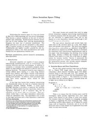
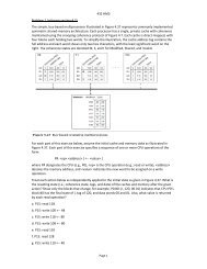
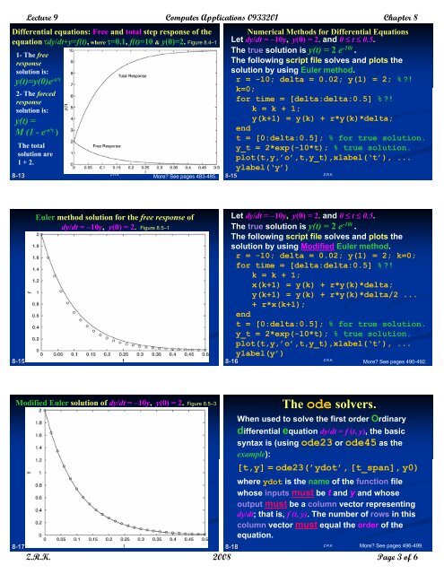
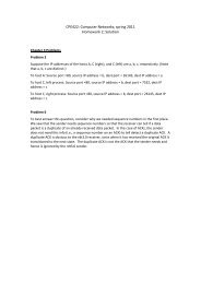
Lecture 9 Computer Applications 0933201 Chapter 8Differential equations: Free and total step response of theequation dy/dt+y=f(t), where =0.1, f(t)=10 & y(0)=2. Figure 8.4–11- The freeresponsesolution is:y(t)=y(0)e -t/2- The forcedresponsesolution is:y(t) =M (1 - e -t/ )The totalsolution are1 + 2.Z.R.K8-13More? See pages 483-485.Numerical Methods for Differential EquationsLet dy/dt = –10y, y(0) = 2. and 0 t 0.5.The true solution is y(t) = 2 e -10t .The following script file solves and plots thesolution by using Euler method.r = -10; delta = 0.02; y(1) = 2; %?!k=0;for time = [delta:delta:0.5] %?!k = k + 1;y(k+1) = y(k) + r*y(k)*delta;endt = [0:delta:0.5]; % for true solution.y_t = 2*exp(-10*t); % true solution.plot(t,y,’o’,t,y_t),xlabel(‘t’), ...ylabel(‘y’)Z.R.K8-15Euler method solution for the free response ofdy/dt = –10y, y(0) = 2. Figure 8.5–1Let dy/dt = –10y, y(0) = 2. and 0 t 0.5.The true solution is y(t) = 2 e -10t .The following script file solves and plots thesolution by using Modified Euler method.r = -10; delta = 0.02; y(1) = 2; k=0;for time = [delta:delta:0.5] %?!k = k + 1;x(k+1) = y(k) + r*y(k)*delta;y(k+1) = y(k) + r*y(k)*delta/2 ...+ r*x(k+1);endt = [0:delta:0.5]; % for true solution.y_t = 2*exp(-10*t); % true solution.plot(t,y,’o’,t,y_t),xlabel(‘t’), ...ylabel(y’)Z.R.K Z.R.K8-158-16More? See pages 490-492.Modified Euler solution of dy/dt = –10y, y(0) = 2. Figure 8.5–3Z.R.K8-17The ode solvers.When used to solve the first order Ordinarydifferential equation dy/dt = f (t, y), the basicsyntax is (using ode23 or ode45 as theexample):[t,y] = ode23(’ydot’, [t_span], y0)where ydot is the name of the function filewhose inputs must be t and y and whoseoutput must be a column vector representingdy/dt; that is, f (t, y). The number of rows in thiscolumn vector must equal the order of theequation.Z.R.K8-18More? See pages 496-499.Z.R.K. 2008 Page 3 of 6