Chapter 17 Radio Propagation Models
Chapter 17 Radio Propagation Models
Chapter 17 Radio Propagation Models

Create successful ePaper yourself
Turn your PDF publications into a flip-book with our unique Google optimized e-Paper software.
<strong>Chapter</strong> <strong>17</strong><br />
<strong>Radio</strong> <strong>Propagation</strong> <strong>Models</strong><br />
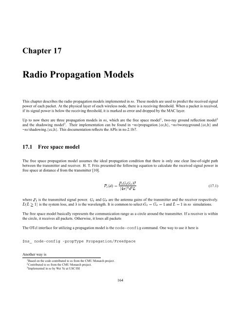
This chapter describes the radio propagation models implemented in ns. These models are used to predict the received signal<br />
power of each packet. At the physical layer of each wireless node, there is a receiving threshold. When a packet is received,<br />
if its signal power is below the receiving threshold, it is marked as error and dropped by the MAC layer.<br />
Up to now there are three propagation models in ns, which are the free space model 1 , two-ray ground reflection model 2<br />
and the shadowing model 3 . Their implementation can be found in ~ns/propagation.{cc,h}, ~ns/tworayground.{cc,h} and<br />
~ns/shadowing.{cc,h}. This documentation reflects the APIs in ns-2.1b7.<br />
<strong>17</strong>.1 Free space model<br />
The free space propagation model assumes the ideal propagation condition that there is only one clear line-of-sight path<br />
between the transmitter and receiver. H. T. Friis presented the following equation to calculate the received signal power in<br />
free space at distance from the transmitter [10].<br />
¢ ¡£<br />
¦ (<strong>17</strong>.1)<br />
¤¥<br />
¡£¢¥¤ §¦©¨<br />
where is the transmitted signal power. and are the antenna gains of the transmitter and the receiver respectively.<br />
¢ ¡£ ¤ ¦ <br />
is the system loss, and is the wavelength. It is common to select and in ns simulations.<br />
¨ ¢¨ ¨ <br />
The free space model basically represents the communication range as a circle around the transmitter. If a receiver is within<br />
the circle, it receives all packets. Otherwise, it loses all packets<br />
The OTcl interface for utilizing a propagation model is the node-config command. One way to use it here is<br />
$ns_ node-config -propType <strong>Propagation</strong>/FreeSpace<br />
Another way is<br />
1 Based on the code contributed to ns from the CMU Monarch project.<br />
2 Contributed to ns from the CMU Monarch project.<br />
3 Implemented in ns by Wei Ye at USC/ISI<br />
164
set prop [new <strong>Propagation</strong>/FreeSpace]<br />
$ns_ node-config -propInstance $prop<br />
<strong>17</strong>.2 Two-ray ground reflection model<br />
A single line-of-sight path between two mobile nodes is seldom the only means of propation. The two-ray ground reflection<br />
model considers both the direct path and a ground reflection path. It is shown [20] that this model gives more accurate<br />
prediction at a long distance than the free space model. The received power at distance is predicted by<br />
¢¡ ¢ <br />
¡£<br />
(<strong>17</strong>.2)<br />
£¢<br />
¡£¢¥¤ §¦©¨<br />
¢<br />
. ¨ where and are the heights of the transmit and receive antennas respectively. Note that the original equation in [20]<br />
assumes To be consistent with the free space model, is added here.<br />
The above equation shows a faster power loss than Eqn. (<strong>17</strong>.1) as distance increases. However, The two-ray model does not<br />
give a good result for a short distance due to the oscillation caused by the constructive and destructive combination of the two<br />
rays. Instead, the free space model is still used when is small.<br />
Therefore, a cross-over distance ¥¤ is calculated in this model. When §¦ ¥¤ , Eqn. (<strong>17</strong>.1) is used. When §¨ ©¤ , Eqn. (<strong>17</strong>.2)<br />
is used. At the cross-over distance, Eqns. (<strong>17</strong>.1) and (<strong>17</strong>.2) give the same result. So ¤ can be calculated as<br />
¤ ¨ ¤ ¥ ¢ ¦ <br />
(<strong>17</strong>.3)<br />
Similarly, the OTcl interface for utilizing the two-ray ground reflection model is as follows.<br />
$ns_ node-config -propType <strong>Propagation</strong>/TwoRayGround<br />
Alternatively, the user can use<br />
set prop [new <strong>Propagation</strong>/TwoRayGround]<br />
$ns_ node-config -propInstance $prop<br />
<strong>17</strong>.3 Shadowing model<br />
<strong>17</strong>.3.1 Backgroud<br />
The free space model and the two-ray model predict the received power as a deterministic function of distance. They both<br />
represent the communication range as an ideal circle. In reality, the received power at certain distance is a random variable<br />
due to multipath propagation effects, which is also known as fading effects. In fact, the above two models predicts the mean<br />
received power at distance . A more general and widely-used model is called the shadowing model [20].<br />
165
¡<br />
Table <strong>17</strong>.1: Some typical values of path loss exponent ¡<br />
Table <strong>17</strong>.2: Some typical values of shadowing deviation §©¨<br />
¡ ¢ ¤ ¦ <br />
¤ ¦ ¡£¢<br />
¡ ¢ ¤ ¦ %<br />
¦'& ¡£¢¥¤<br />
<br />
<br />
Environment<br />
Outdoor Free space 2<br />
Shadowed urban area 2.7 to 5<br />
In building Line-of-sight 1.6 to 1.8<br />
Obstructed 4 to 6<br />
Environment<br />
Outdoor 4 to 12<br />
¢¤£¦¥ (dB)<br />
Office, hard partition 7<br />
Office, soft partition 9.6<br />
Factory, line-of-sight 3 to 6<br />
Factory, obstructed 6.8<br />
The shadowing model consists of two parts. The first one is known as path loss model, which also predicts the mean received<br />
power at distance , denoted by . It uses a close-in distance as a reference. is computed relative to as<br />
¢ ¤ §¦ ¡ ¢ ¤ ¦<br />
follows.<br />
¡ §¦ ¤ ¢ ¡<br />
¡£¢¥¤ ¦<br />
(<strong>17</strong>.4)<br />
¨<br />
¡ ¢ ¤ §¦<br />
is called the path loss exponent, and is usually empirically determined by field measurement. From Eqn.<br />
¨<br />
¡ (<strong>17</strong>.1) we know that<br />
for free space propagation. Table <strong>17</strong>.1 ¡ gives some typical values of . Larger values correspond to more obstructions<br />
and hence faster decrease in average received power as distance becomes larger. can be computed from Eqn. (<strong>17</strong>.1).<br />
¦ ¤ ¢ ¡<br />
The path loss is usually measured in dB. So from Eqn. (<strong>17</strong>.4) we have<br />
$ (<strong>17</strong>.5)<br />
¨ <br />
¡! #"<br />
¨<br />
The second part of the shadowing model reflects the variation of the received power at certain distance. It is a log-normal<br />
random variable, that is, it is of Gaussian distribution if measured in dB. The overall shadowing model is represented by<br />
*),+ ¨ (<strong>17</strong>.6)<br />
¨( <br />
¡! #"<br />
¨<br />
where + ¨ is a Gaussian random variable with zero mean and standard deviation § ¨ . § ¨ is called the shadowing deviation,<br />
and is also obtained by measurement. Table <strong>17</strong>.2 shows some typical values of § ¨ . Eqn. (<strong>17</strong>.6) is also known as a log-normal<br />
shadowing model.<br />
The shadowing model extends the ideal circle model to a richer statistic model: nodes can only probabilistically communicate<br />
when near the edge of the communication range.<br />
166
<strong>17</strong>.3.2 Using shadowing model<br />
Before using the model, the user should select the values of the path loss ¡ exponent<br />
according to the simulated environment.<br />
and the shadowing deviation § ¨<br />
The OTcl interface is still the node-config command. One way to use it is as follows, and the values for these parameters<br />
are just examples.<br />
# first set values of shadowing model<br />
<strong>Propagation</strong>/Shadowing set pathlossExp_ 2.0<br />
<strong>Propagation</strong>/Shadowing set std_db_ 4.0<br />
<strong>Propagation</strong>/Shadowing set dist0_ 1.0<br />
<strong>Propagation</strong>/Shadowing set seed_ 0<br />
;# path loss exponent<br />
;# shadowing deviation (dB)<br />
;# reference distance (m)<br />
;# seed for RNG<br />
$ns_ node-config -propType <strong>Propagation</strong>/Shadowing<br />
The shadowing model creates a random number generator (RNG) object. The RNG has three types of seeds: raw seed,<br />
pre-defined seed (a set of known good seeds) and the huristic seed (details in Section 20.1). The above API only uses the<br />
pre-defined seed. If a user want different seeding method, the following API can be used.<br />
set prop [new <strong>Propagation</strong>/Shadowing]<br />
$prop set pathlossExp_ 2.0<br />
$prop set std_db_ 4.0<br />
$prop set dist0_ 1.0<br />
$prop seed 0<br />
;# user can specify seeding method<br />
$ns_ node-config -propInstance $prop<br />
The above can be raw, predef or heuristic.<br />
<strong>17</strong>.4 Communication range<br />
In some applications, a user may want to specify the communication range of wireless nodes. This can be done by set an<br />
appropriate value of the receiving threshold in the network interface, i.e.,<br />
Phy/WirelessPhy set RXThresh_ <br />
A separate C program is provided at ~ns/indep-utils/propagation/threshold.cc to compute the receiving threshold. It can be<br />
used for all the propagation models discussed in this chapter. Assume you have compiled it and get the excutable named as<br />
threshold. You can use it to compute the threshold as follows<br />
threshold -m [other-options] distance<br />
where is either FreeSpace, TwoRayGround or Shadowing, and the distance is the<br />
communication range in meter.<br />
167
[other-options] are used to specify parameters other than their default values. For the shadowing model there is a<br />
necessary parameter, -r , which specifies the rate of correct reception at the distance. Because<br />
the communication range in the shadowing model is not an ideal circle, an inverse Q-function [20] is used to calculate the<br />
receiving threshold. For example, if you want 95% of packets can be correctly received at the distance of 50m, you can<br />
compute the threshold by<br />
threshold -m Shadowing -r 0.95 50<br />
Other available values of [other-options] are shown below<br />
-pl -std -Pt <br />
-fr -Gt -Gr <br />
-L -ht -hr <br />
-d0 <br />
<strong>17</strong>.5 Commands at a glance<br />
Following is a list of commands for propagation models.<br />
$ns_ node-config -propType <br />
This command selects in the simulation. the can be<br />
<strong>Propagation</strong>/FreeSpace, <strong>Propagation</strong>/TwoRayGround or <strong>Propagation</strong>/Shadowing<br />
$ns_ node-config -propInstance $prop<br />
This command is another way to utilize a propagation model. $prop is an instance of the .<br />
$sprop_ seed <br />
This command seeds the RNG. $sprop_ is an instance of the shadowing model.<br />
threshold -m [other-options] distance<br />
This is a separate program at ~ns/indep-utils/propagation/threshold.cc, which is used to compute the receiving threshold for<br />
a specified communication range.<br />
168
![Problem 1: Loop Unrolling [18 points] In this problem, we will use the ...](https://img.yumpu.com/36629594/1/184x260/problem-1-loop-unrolling-18-points-in-this-problem-we-will-use-the-.jpg?quality=85)