original version printed in the x-ray data booklet

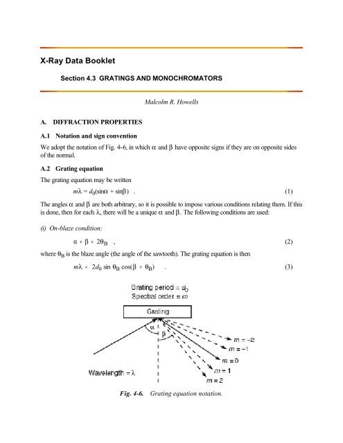
X-Ray Data BookletSection 4.3 GRATINGS AND MONOCHROMATORSMalcolm R. HowellsA. DIFFRACTION PROPERTIESA.1 Notation and sign conventionWe adopt the notation of Fig. 4-6, in which α and β have opposite signs if they are on opposite sidesof the normal.A.2 Grating equationThe grating equation may be writtenmλ = d 0 (sinα + sinβ) . (1)The angles α and β are both arbitrary, so it is possible to impose various conditions relating them. If thisis done, then for each λ, there will be a unique α and β. The following conditions are used:(i) On-blaze condition:α + β = 2θ B , (2)where θ B is the blaze angle (the angle of the sawtooth). The grating equation is thenmλ = 2d 0 sin θ B cos(β + θ B ) . (3)Fig. 4-6. Grating equation notation.

(ii) Fixed in and out directions:α − β = 2θ , (4)where 2θ is the (constant) included angle. The grating equation is thenmλ = 2d 0 cosθsin( θ + β) . (5)In this case, the wavelength scan ends when α or β reaches 90°, which occurs at the horizonwavelength λ H = 2d 0 cos 2 θ.(iii) Constant incidence angle: Equation (1) gives β directly.(iv) Constant focal distance (of a plane grating):leading to a grating equationcos βcosα = a constant c ff , (6)⎛1 – ⎜mλ⎝ d– sin β⎞⎟⎠2=cos 2 βc ff2. (7)Equations (3), (5), and (7) give β (and thence α) for any λ. Examples of the above α-βrelationships are (for references see http://www-cxro.lbl.gov/):(i) Kunz et al. plane-grating monochromator (PGM), Hunter et al. double PGM, collimated-lightSX700 PGM(ii) Toroidal-grating monochromators (TGMs), spherical-grating monochromators (SGMs, “Dragon”system), Seya-Namioka, most aberration-reduced holographic SGMs, variable-angle SGM,PGMs(iii) Spectrographs, “Grasshopper” monochromator(iv) Standard SX700 PGM and most variantsB. FOCUSING PROPERTIESThe study of diffraction gratings (for references see http://www-cxro.lbl.gov/) goes back more than acentury and has included plane, spherical [1], toroidal, and ellipsoidal surfaces and groove patternsmade by classical (“Rowland”) ruling [2], holography [3,4], and variably spaced ruling [5,6]. In recentyears the optical design possibilities of holographic groove patterns and variably spaced rulings havebeen extensively developed. Following normal practice, we provide an analysis of the imagingproperties of gratings by means of the path function F [7]. For this purpose we use the notation of Fig.4-7, in which the zeroth groove (of width d 0 ) passes through the grating pole O, while the nth groovepasses through the variable point P(ξ,w,l). The holographic groove pattern is taken to be made usingtwo coherent point sources C and D with cylindrical polar coordinates (r C ,γ,z C ), (r D ,δ,z D ) relative toO. The lower (upper) sign in Eq. (9) refers to C and D both real or both virtual (one real and onevirtual), for which case the equiphase surfaces are confocal hyperboloids (ellipses) of revolution about

CD. Gratings with varied line spacing d(w) are assumed to be ruled according to d(w) = d 0 (1 + v 1 w +v 2 w2 + ...).Fig. 4-7. Focusing properties notation.We consider all the gratings to be ruled on the general surfacex =∑ija ij w i l jand the a ij coefficients are given below.Ellipse coefficients a ija 20 =cosθ4⎛ 1r + 1 ⎞⎝ r ′ ⎠a 12 =a 30 = a 20 A a 22 =a 40 =a 20 ( 4 A2 + C)4a 04 =a 20 Acos 2 θa 20 ( 2 A 2 + C)2cos 2 θa 20 C8cos 2 θa 02 =a 20cos 2 θThe other a ij ’s with i + j ≤ 4 are zero. In the expressions above, r, r ′ , and θ are the object distance,image distance, and incidence angle to the normal, respectively, andA = sin θ2⎛ 1r – 1 ⎞⎝ r ′ ⎠, C = A 2 +1r r ′.

Toroid coefficients a ija 20 =a 40 =12Ra 22 =18R 3 a 04 =14ρR 218ρ 3a 02 =12ρOther a ij ’s with i + j ≤ 4 are zero. Here, R and ρ are the major and minor radii of the bicycle-tiretoroid.The a ij ’s for spheres; circular, parabolic, and hyperbolic cylinders; paraboloids; and hyperboloidscan also be obtained from the values above by suitable choices of the input parameters r, r ′ , and θ .Values for the ellipse and toroid coefficients are given to sixth order at http://www-cxro.lbl.gov/.B.1 Calculation of the path function FF is expressed asF = ∑F ijk w i l j , (8)ijkwhereF ijk = z k C ijk (α ,r) + z ′ k C ijk (β, r ′ ) + mλ fd ijk0and the f ijk term, originating from the groove pattern, is given by one of the following expressions:f ijk =⎧ 1 when ijk = 100, 0 otherwise Rowland⎪⎪ d 0⎨ z k λ C C ijk (γ , r C ) ± z k D C ijk (δ, r D )0[ ] holographic⎪⎪⎩ n ijkvaried line spacingThe coefficient F ijk is related to the strength of the i,j aberration of the wavefront diffracted by thegrating. The coefficients C ijk and n ijk are given below, where the following notation is used:andT = T (r,α ) =S = S(r,α ) =cos 2 αr– 2a 20 cosα (10a)1r – 2a 02 cosα . (10b)Coefficients C ijk of the expansion of F(9)

C 011 = – 1 rC 031 =C 100 = − sin αC 020 =S2C 022 = –S2r 2 C 040 =C 102 = sin α2r 2C 111 = − sin αr 2 C 120 =C 200 =T2S4r 2 – 12r 34a 2 02– S 28rSsin α2r− a 04 cosα– a 12 cosαC 202 = − T4r 2 + sin 2 α2r 3C 211 =T2r 2 − sin 2 αr 3C 300 = −a 30 cosα + T sin α2rC 220 = − a 22 cosα +1( 4r 4a 20 a 02 − TS − 2a 12 sin 2α )+ S sin 2 α2 r 2C 400 = −a 40 cosα +1(8r 4a 202 − T 2 − 4a 30 sin 2α )+ T sin 2 α2r 2The coefficients for which i ≤ 4, j ≤ 4, k ≤ 2, i + j + k ≤ 4,j + k = even are included here.Coefficients n ijk of the expansion of Fn ijk = 0 for j, k ≠ 0n 100 = 1 n 300 =v 1 2 − v 23n 200 =−v 12n 400 =−v 1 3 + 2v 1 v 2 − v 34Values for C ijk and n ijk are given to sixth order at http://www-cxro.lbl.gov/.B.2 Determination of the Gaussian image pointBy definition the principal ray AOB 0 arrives at the Gaussian image point B 0 ( r 0 ′ , β 0 , z ′ 0 ) in Fig. 4-7. Itsdirection is given by Fermat’s principal, which implies [∂F/∂w] w=0,l=0 = 0 and [∂F/∂l] w=0,l=0 = 0, fromwhichandmλd 0= sin α + sin β 0 (11a)

zr + z ′ 0= 0 , (11b)r 0 ′which are the grating equation and the law of magnification in the vertical direction. The tangential focaldistance r 0 ′ is obtained by setting the focusing term F 200 equal to zero and is given byT (r,α ) + T ( r 0 ′ , β 0 ) =⎧0⎪Rowland⎪⎨ – mλ [T(rλ C ,γ ) ±T(r D ,δ)]⎪ 0holographic⎪ v l mλ⎩⎪varied line spacingd 0Equations (11) and (12) determine the Gaussian image point B 0 and, in combination with the sagittalfocusing condition (F 020 = 0), describe the focusing properties of grating systems under the paraxialapproximation. For a Rowland spherical grating the focusing condition, Eq. (12), is⎛⎜ cos 2 α⎝ r− cosαR⎞⎠ +⎛⎜cos 2 β⎝ r 0 ′− cos βRwhich has important special cases: (i) plane grating, R = ∞ ,implyingr 0 ′ = –r cos 2 α/cos 2 β = –r/c2ff(12)⎞⎟ = 0 , (13)⎠so that the focal distance and magnification are fixed if c ff is held constant; (ii) object and image on theRowland circle, i.e., r = Rcosα , r 0 ′ = R cosβ , M = l; and (iii) β = 90° (Wadsworth condition). Thefocal distances of TGMs and SGMs, with or without moving slits, are also determined using Eq. (13).B.3 Calculation of ray aberrationsIn an aberrated system, the outgoing ray will arrive at the Gaussian image plane at a point B R displacedfrom the Gaussian image point B 0 by the ray aberrations ∆ y ′ and ∆ z ′ (Fig. 4-7). The latter are givenby∆ y ′ =r 0 ′ ∂Fcosβ 0 ∂w , ∆ z ′ = r 0 ′ ∂F∂l, (14)where F is to be evaluated for A = (r,α,z) and B = ( r 0 ′ ,β 0 , z 0 ′ ). By means of the expansion of F,these equations allow the ray aberrations to be calculated separately for each aberration type:∆ y ′ ijk =r 0 ′Fcos β ijk iw i–1 l j , ∆ z ′ ijk = r 0 ′ F ijk w i jl j –1 . (15)0Moreover, provided the aberrations are not too large, they are additive, so that they may eitherreinforce or cancel.

C. DISPERSION PROPERTIESDispersion properties can be summarized by the following relations.(i) Angular dispersion:⎛⎜∂λ ⎞ ⎟⎝ ∂β ⎠α=d cosβm. (16)(ii) Reciprocal linear dispersion:⎛ ⎜ ∂λ ⎞=⎝ ∂(∆ y ′ ) ⎠ αd cosβm r ′≡ 10–3 d[Å]cosβm r ′ [m]Å/mm . (17)(iii) Magnification:M(λ) =cosαcos βr ′r. (18)(iv) Phase-space acceptance (ε):ε = N∆λ S1 = N∆λ S2 (assuming S 2 = MS 1 ) , (19)where N is the number of participating grooves.D. RESOLUTION PROPERTIESThe following are the main contributions to the width of the instrumental line spread function. Anestimate of the total width is the vector sum.(i) Entrance slit (width S 1 ):∆λ S1 =S 1 d cosαmr. (20)(ii) Exit slit (width S 2 ):∆λ S2 =S 2 d cosβm r ′. (21)(iii) Aberrations (of perfectly made grating):∆λ A =∆ y ′ d cos β=m r ′dm⎛ ∂F ⎞⎝ ∂w⎠. (22)(iv) Slope error ∆φ (of imperfectly made grating):

∆λ SE =d(cosα + cos β)∆φm. (23)Note that, provided the grating is large enough, diffraction at the entrance slit always guarantees acoherent illumination of enough grooves to achieve the slit-width-limited resolution. In such case adiffraction contribution to the width need not be added to the above.E. EFFICIENCYThe most accurate way to calculate grating efficiencies is by the full electromagnetic theory [8].However, approximate scalar-theory calculations are often useful and, in particular, provide a way tochoose the groove depth h of a laminar grating. According to Bennett, the best value of the groovewidth-to-periodratio r is the one for which the usefully illuminated area of the groove bottom is equal tothat of the top. The scalar-theory efficiency of a laminar grating with r = 0.5 is given by Franks et al. asE 0 =R4⎡⎛ 4πh cosα1 + 2(1 – P) cos⎣ ⎢⎝ λ⎞⎠⎤+ (1 – P)2⎦ ⎥whereE m =P =⎧ Rm 2 π 2 [1 – 2 cosQ+ cos(Q – + δ)⎪⎪ + cos 2 Q + ] m = odd⎨⎪ R⎪ m 2 π 2 cos2 Q +m = even⎩4h tanαd 0,(24)Q ± =mπhd 0(tanα ± tan β) ,δ =2πh(cosα + cosβ ) ,λand R is the reflectance at grazing angle α G β G ,whereα G =π2 − | α | and β G = π2 − | β | .REFERENCES1. H. G. Beutler, “The Theory of the Concave Grating,” J. Opt. Soc. Am. 35, 311 (1945).