L - X-Ray Data Booklet - Lawrence Berkeley National Laboratory
L - X-Ray Data Booklet - Lawrence Berkeley National Laboratory
L - X-Ray Data Booklet - Lawrence Berkeley National Laboratory

Create successful ePaper yourself
Turn your PDF publications into a flip-book with our unique Google optimized e-Paper software.
X-<strong>Ray</strong> <strong>Data</strong> <strong>Booklet</strong><br />
X-RAY DATA BOOKLET<br />
Center for X-ray Optics and Advanced Light Source<br />
<strong>Lawrence</strong> <strong>Berkeley</strong> <strong>National</strong> <strong>Laboratory</strong><br />
Introduction<br />
X-<strong>Ray</strong> Properties of<br />
Elements<br />
Now Available<br />
Order X-<strong>Ray</strong> <strong>Data</strong> <strong>Booklet</strong><br />
Electron Binding Energies<br />
X-<strong>Ray</strong> Energy Emission<br />
Energies<br />
Fluorescence Yields for K and<br />
L Shells<br />
Principal Auger Electron<br />
Energies<br />
Subshell Photoionization<br />
Cross-Sections<br />
Mass Absorption Coefficients<br />
Atomic Scattering Factors<br />
Energy Levels of Few<br />
Electron Ions<br />
http://xdb.lbl.gov/ (1 of 3) [2/14/2005 6:47:36 PM]
X-<strong>Ray</strong> <strong>Data</strong> <strong>Booklet</strong><br />
Periodic Table of X-<strong>Ray</strong><br />
Properties<br />
Synchrotron Radiation<br />
Characteristics of Synchrotron<br />
Radiation<br />
History of X-rays and<br />
Synchrotron Radiation<br />
Synchrotron Facilities<br />
Scattering Processes<br />
Scattering of X-rays from<br />
Electrons and Atoms<br />
Low-Energy Electron Ranges<br />
in Matter<br />
Optics and Detectors<br />
Crystal and Multilayer<br />
Elements<br />
Specular Reflectivities for<br />
Grazing-Incidence Mirrors<br />
Gratings and Monochromators<br />
Zone Plates<br />
X-<strong>Ray</strong> Detectors<br />
Miscellaneous<br />
http://xdb.lbl.gov/ (2 of 3) [2/14/2005 6:47:36 PM]
X-<strong>Ray</strong> <strong>Data</strong> <strong>Booklet</strong><br />
Physical Constants<br />
Physical Properties of the<br />
Elements<br />
Electromagnetic Relations<br />
Radioactivity and Radiation<br />
Protection<br />
Useful Formulas<br />
CXRO Home | ALS Home | LBL Home<br />
Privacy and Security Notice<br />
Please send comments or questions to acthompson@lbl.gov ©2000<br />
http://xdb.lbl.gov/ (3 of 3) [2/14/2005 6:47:36 PM]
Section 1 X-<strong>Ray</strong> Properties of the Elements<br />
Introduction<br />
Preface in PDF format<br />
<strong>Data</strong> <strong>Booklet</strong> Authors<br />
CXRO Home | ALS Home | LBL Home<br />
Privacy and Security Notice<br />
Please send comments or questions to acthompson@lbl.gov ©2000<br />
http://xdb.lbl.gov/Intro/index.html [2/14/2005 6:47:37 PM]
C E N T E R F O R X - R A Y O P T I C S<br />
A D V A N C E D L I G H T S O U R C E<br />
X-RAY DATA BOOKLET<br />
Albert C. Thompson, David T. Attwood, Eric M.<br />
Gullikson, Malcolm R. Howells, Jeffrey B. Kortright,<br />
Arthur L. Robinson, and James H. Underwood<br />
—<strong>Lawrence</strong> <strong>Berkeley</strong> <strong>National</strong> <strong>Laboratory</strong><br />
Kwang-Je Kim<br />
—Argonne <strong>National</strong> <strong>Laboratory</strong><br />
Janos Kirz<br />
—State University of New York at Stony Brook<br />
Ingolf Lindau, Piero Pianetta, and Herman Winick<br />
—Stanford Synchrotron Radiation <strong>Laboratory</strong><br />
Gwyn P. Williams<br />
—Brookhaven <strong>National</strong> <strong>Laboratory</strong><br />
James H. Scofield<br />
—<strong>Lawrence</strong> Livermore <strong>National</strong> <strong>Laboratory</strong><br />
Compiled and edited by<br />
Albert C. Thompson and Douglas Vaughan<br />
—<strong>Lawrence</strong> <strong>Berkeley</strong> <strong>National</strong> <strong>Laboratory</strong><br />
<strong>Lawrence</strong> <strong>Berkeley</strong> <strong>National</strong> <strong>Laboratory</strong><br />
University of California<br />
<strong>Berkeley</strong>, California 94720<br />
Second edition, January 2001<br />
This work was supported in part by the U.S. Department of Energy<br />
under Contract No. DE-AC03-76SF00098
CONTENTS<br />
1. X-<strong>Ray</strong> Properties of the Elements 1-1<br />
1.1 Electron Binding Energies<br />
Gwyn P. Williams 1-1<br />
1.2 X-<strong>Ray</strong> Emission Energies<br />
Jeffrey B. Kortright and<br />
Albert C. Thompson 1-8<br />
1.3 Fluorescence Yields For K and L Shells<br />
Jeffrey B. Kortright 1-28<br />
1.4 Principal Auger Electron Energies 1-30<br />
1.5 Subshell Photoionization Cross Sections<br />
Ingolf Lindau 1-32<br />
1.6 Mass Absorption Coefficients<br />
Eric M. Gullikson 1-38<br />
1.7 Atomic Scattering Factors<br />
Eric M. Gullikson 1-44<br />
1.8 Energy Levels of Few-Electron Ionic Species<br />
James H. Scofield 1-53<br />
2. Synchrot ron Radiation 2-1<br />
2.1 Characteristics of Synchrotron Radiation<br />
Kwang-Je Kim 2-1<br />
2.2 History of Synchrotron Radiation<br />
Arthur L. Robinson 2-17<br />
2.3 Operating and Planned Facilities<br />
Herman Winick 2-24
3. Scattering Processes 3-1<br />
3.1 Scattering of X-<strong>Ray</strong>s from Electrons and Atoms<br />
Janos Kirz 3-1<br />
3.2 Low-Energy Electron Ranges In Matter<br />
Piero Pianetta 3-5<br />
4. Optics and Detectors 4-1<br />
4.1 Multilayers and Crystals<br />
James H. Underwood 4-1<br />
4.2 Specular Reflectivities for Grazing-Incidence Mirrors<br />
Eric M. Gullikson 4-14<br />
4.3 Gratings and Monochromators<br />
Malcolm R. Howells 4-17<br />
4.4 Zone Plates<br />
Janos Kirz and David Attwood 4-28<br />
4.5 X-<strong>Ray</strong> Detectors<br />
Albert C. Thompson 4-33<br />
5. Miscellaneous 5-1<br />
5.1 Physical Constants 5-1<br />
5.2 Physical Properties of the Elements 5-4<br />
5.3 Electromagnetic Relations 5-11<br />
5.4 Radioactivity and Radiation Protection 5-14<br />
5.5 Useful Equations 5-17
PREFACE<br />
For the first time since its original publication in 1985, the<br />
X-<strong>Ray</strong> <strong>Data</strong> <strong>Booklet</strong> has undergone a significant revision.<br />
Tabulated values and graphical plots have been revised and<br />
updated, and the content has been modified to reflect the<br />
changing needs of the x-ray community. Further, the <strong>Booklet</strong> is<br />
now posted on the web at http://xdb.lbl.gov, together with additional<br />
detail and further references for many of the sections.<br />
As before, the compilers are grateful to a host of contributors<br />
who furnished new material or reviewed and revised their<br />
original sections. Also, as in the original edition, many sections<br />
draw heavily on work published elsewhere, as indicated in the<br />
text and figure captions. Thanks also to Linda Geniesse,<br />
Connie Silva, and Jean Wolslegel of the LBNL Technical and<br />
Electronic Information Department, whose skills were invaluable<br />
and their patience apparently unlimited. Finally, we express<br />
continuing thanks to David Attwood for his support of<br />
this project, as well as his contributions to the <strong>Booklet</strong>, and to<br />
Janos Kirz, who conceived the <strong>Booklet</strong> as a service to the<br />
community and who remains an active contributor to the<br />
second edition.<br />
As the compilers, we take full responsibility for any errors<br />
in this new edition, and we invite readers to bring them to our<br />
attention at the Center for X-<strong>Ray</strong> Optics, 2-400, <strong>Lawrence</strong><br />
<strong>Berkeley</strong> <strong>National</strong> <strong>Laboratory</strong>, <strong>Berkeley</strong>, California 94720, or<br />
by e-mail at xdb@grace.lbl.gov. Corrections will be posted on<br />
the web and incorporated in subsequent printings.<br />
Albert C. Thompson<br />
Douglas Vaughan<br />
31 January 2001
<strong>Data</strong> <strong>Booklet</strong> Authors<br />
X-<strong>Ray</strong> <strong>Data</strong> <strong>Booklet</strong> Authors<br />
Al Thompson and Doug Vaughan<br />
Second Edition Editors<br />
http://xdb.lbl.gov/Intro/<strong>Booklet</strong>_Authors.htm (1 of 3) [2/14/2005 6:47:38 PM]
<strong>Data</strong> <strong>Booklet</strong> Authors<br />
http://xdb.lbl.gov/Intro/<strong>Booklet</strong>_Authors.htm (2 of 3) [2/14/2005 6:47:38 PM]
<strong>Data</strong> <strong>Booklet</strong> Authors<br />
http://xdb.lbl.gov/Intro/<strong>Booklet</strong>_Authors.htm (3 of 3) [2/14/2005 6:47:38 PM]
Section 1 X-<strong>Ray</strong> Properties of the Elements<br />
1. X-<strong>Ray</strong> Properties of the Elements<br />
Contents<br />
Electron Binding Energies- Gwyn P. Williams<br />
X-<strong>Ray</strong> Energy Emission Energies<br />
- Jeffrey B. Kortright and Albert C. Thompson<br />
Fluorescence Yields for K and L Shells - Jeffrey B. Kortright<br />
Principal Auger Electron Energies<br />
Subshell Photoionization Cross-Sections - Ingolf Lindau<br />
Mass Absorption Coefficients - Eric M. Gullikson<br />
Atomic Scattering Factors - Eric M. Gullikson<br />
Energy Levels of Few Electron Ions - James H. Scofield<br />
Periodic Table of X-<strong>Ray</strong> Properties - Albert C. Thompson<br />
CXRO Home | ALS Home | LBL Home<br />
Privacy and Security Notice<br />
Please send comments or questions to acthompson@lbl.gov ©2000<br />
http://xdb.lbl.gov/Section1/index.html [2/14/2005 6:47:38 PM]
1<br />
X-<strong>Ray</strong> <strong>Data</strong> <strong>Booklet</strong><br />
Section 1.1 ELECTRON BINDING ENERGIES<br />
Gwyn P. Williams<br />
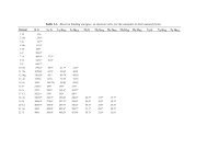
Table 1-1 gives the electron binding energies for the elements in their natural<br />
forms. A PDF version of this table is also available. The energies are given in<br />
electron volts relative to the vacuum level for the rare gases and for H 2 , N 2 , O 2 ,<br />
F 2 , and Cl 2 ; relative to the Fermi level for the metals; and relative to the top of<br />
the valence bands for semiconductors. Values have been taken from Ref. 1 except<br />
as follows:<br />
* Values taken from Ref. 2, with additional corrections<br />
† Values taken from Ref. 3.<br />
a One-particle approximation not valid owing to short core-hole lifetime.<br />
b Value derived from Ref. 1.<br />
Thanks also to R. Johnson, G. Ice, M. Olmstead, P. Dowben, M. Seah, E.<br />
Gullikson, F. Boscherini, W. O’Brien, R. Alkire, and others.<br />
REFERENCES<br />
1. J. A. Bearden and A. F. Burr, “Reevaluation of X-<strong>Ray</strong> Atomic Energy<br />
Levels,” Rev. Mod. Phys. 39, 125 (1967).<br />
2. M. Cardona and L. Ley, Eds., Photoemission in Solids I: General<br />
Principles (Springer-Verlag, Berlin, 1978).<br />
3. J. C. Fuggle and N. Mårtensson, “Core-Level Binding Energies in<br />
Metals,” J. Electron Spectrosc. Relat. Phenom. 21, 275 (1980).<br />
Elements Hydrogen (1) to Ag (47)<br />
Elements Cadmium (48) to Ytterbium(70)<br />
Elements Lutetium (71) to Uranium (92)<br />
http://xdb.lbl.gov/Section1/Sec_1-1.html (1 of 2) [2/14/2005 6:47:38 PM]
1<br />
http://xdb.lbl.gov/Section1/Sec_1-1.html (2 of 2) [2/14/2005 6:47:38 PM]
Table 1-1. Electron binding energies, in electron volts, for the elements in their natural forms.<br />
Element K 1s L 1 2s L 2 2p 1/2 L 3 2p 3/2 M 1 3s M 2 3p 1/2 M 3 3p 3/2 M 4 3d 3/2 M 5 3d 5/2 N 1 4s N 2 4p 1/2 N 3 4p 3/2<br />
1 H 13.6<br />
2 He 24.6*<br />
3 Li 54.7*<br />
4 Be 111.5*<br />
5 B 188*<br />
6 C 284.2*<br />
7 N 409.9* 37.3*<br />
8 O 543.1* 41.6*<br />
9 F 696.7*<br />
10 Ne 870.2* 48.5* 21.7* 21.6*<br />
11 Na 1070.8† 63.5† 30.65 30.81<br />
12 Mg 1303.0† 88.7 49.78 49.50<br />
13 Al 1559.6 117.8 72.95 72.55<br />
14 Si 1839 149.7*b 99.82 99.42<br />
15 P 2145.5 189* 136* 135*<br />
16 S 2472 230.9 163.6* 162.5*<br />
17 Cl 2822.4 270* 202* 200*<br />
18 Ar 3205.9* 326.3* 250.6† 248.4* 29.3* 15.9* 15.7*<br />
19 K 3608.4* 378.6* 297.3* 294.6* 34.8* 18.3* 18.3*<br />
20 Ca 4038.5* 438.4† 349.7† 346.2† 44.3 † 25.4† 25.4†<br />
21 Sc 4492 498.0* 403.6* 398.7* 51.1* 28.3* 28.3*<br />
22 Ti 4966 560.9† 460.2† 453.8† 58.7† 32.6† 32.6†
23 V 5465 626.7† 519.8† 512.1† 66.3† 37.2† 37.2†<br />
24 Cr 5989 696.0† 583.8† 574.1† 74.1† 42.2† 42.2†<br />
25 Mn 6539 769.1† 649.9† 638.7† 82.3† 47.2† 47.2†<br />
26 Fe 7112 844.6† 719.9† 706.8† 91.3† 52.7† 52.7†<br />
27 Co 7709 925.1† 793.2† 778.1† 101.0† 58.9† 59.9†<br />
28 Ni 8333 1008.6† 870.0† 852.7† 110.8† 68.0† 66.2†<br />
29 Cu 8979 1096.7† 952.3† 932.7 122.5† 77.3† 75.1†<br />
30 Zn 9659 1196.2* 1044.9* 1021.8* 139.8* 91.4* 88.6* 10.2* 10.1*<br />
31 Ga 10367 1299.0*b 1143.2† 1116.4† 159.5† 103.5† 100.0† 18.7† 18.7†<br />
32 Ge 11103 1414.6*b 1248.1*b 1217.0*b 180.1* 124.9* 120.8* 29.8 29.2<br />
33 As 11867 1527.0*b 1359.1*b 1323.6*b 204.7* 146.2* 141.2* 41.7* 41.7*<br />
34 Se 12658 1652.0*b 1474.3*b 1433.9*b 229.6* 166.5* 160.7* 55.5* 54.6*<br />
35 Br 13474 1782* 1596* 1550* 257* 189* 182* 70* 69*<br />
36 Kr 14326 1921 1730.9* 1678.4* 292.8* 222.2* 214.4 95.0* 93.8* 27.5* 14.1* 14.1*<br />
37 Rb 15200 2065 1864 1804 326.7* 248.7* 239.1* 113.0* 112* 30.5* 16.3* 15.3 *<br />
38 Sr 16105 2216 2007 1940 358.7† 280.3† 270.0† 136.0† 134.2† 38.9† 21.3 20.1†<br />
39 Y 17038 2373 2156 2080 392.0*b 310.6* 298.8* 157.7† 155.8† 43.8* 24.4* 23.1*<br />
40 Zr 17998 2532 2307 2223 430.3† 343.5† 329.8† 181.1† 178.8† 50.6† 28.5† 27.1†<br />
41 Nb 18986 2698 2465 2371 466.6† 376.1† 360.6† 205.0† 202.3† 56.4† 32.6† 30.8†<br />
42 Mo 20000 2866 2625 2520 506.3† 411.6† 394.0† 231.1† 227.9† 63.2† 37.6† 35.5†<br />
43 Tc 21044 3043 2793 2677 544* 447.6 417.7 257.6 253.9* 69.5* 42.3* 39.9*<br />
44 Ru 22117 3224 2967 2838 586.1* 483.5† 461.4† 284.2† 280.0† 75.0† 46.3† 43.2†<br />
45 Rh 23220 3412 3146 3004 628.1† 521.3† 496.5† 311.9† 307.2† 81.4*b 50.5† 47.3†<br />
46 Pd 24350 3604 3330 3173 671.6† 559.9† 532.3† 340.5† 335.2† 87.1*b 55.7†a 50.9†<br />
47 Ag 25514 3806 3524 3351 719.0† 603.8† 573.0† 374.0† 368.3 97.0† 63.7† 58.3†
Table 1-1. Electron binding energies (continued).<br />
Element K 1s L 1 2s L 2 2p 1/2 L 3 2p 3/2 M 1 3s M 2 3p 1/2 M 3 3p 3/2 M 4 3d 3/2 M 5 3d 5/2 N 1 4s N 2 4p 1/2 N 3 4p 3/2<br />
48 Cd 26711 4018 3727 3538 772.0† 652.6† 618.4† 411.9† 405.2† 109.8† 63.9†a 63.9†a<br />
49 In 27940 4238 3938 3730 827.2† 703.2† 665.3† 451.4† 443.9† 122.9† 73.5†a 73.5†a<br />
50 Sn 29200 4465 4156 3929 884.7† 756.5† 714.6† 493.2† 484.9† 137.1† 83.6†a 83.6†a<br />
51 Sb 30491 4698 4380 4132 946† 812.7† 766.4† 537.5† 528.2† 153.2† 95.6†a 95.6†a<br />
52 Te 31814 4939 4612 4341 1006† 870.8† 820.0† 583.4† 573.0† 169.4† 103.3†a 103.3†a<br />
53 I 33169 5188 4852 4557 1072* 931* 875* 630.8 619.3 186* 123* 123*<br />
54 Xe 34561 5453 5107 4786 1148.7* 1002.1* 940.6* 689.0* 676.4* 213.2* 146.7 145.5*<br />
55 Cs 35985 5714 5359 5012 1211*b 1071* 1003* 740.5* 726.6* 232.3* 172.4* 161.3*<br />
56 Ba 37441 5989 5624 5247 1293*b 1137*b 1063*b 795.7† 780.5* 253.5† 192 178.6†<br />
57 La 38925 6266 5891 5483 1362*b 1209*b 1128*b 853* 836* 274.7* 205.8 196.0*<br />
58 Ce 40443 6549 6164 5723 1436*b 1274*b 1187*b 902.4* 883.8* 291.0* 223.2 206.5*<br />
59 Pr 41991 6835 6440 5964 1511 1337 1242 948.3* 928.8* 304.5 236.3 217.6<br />
60 Nd 43569 7126 6722 6208 1575 1403 1297 1003.3* 980.4* 319.2* 243.3 224.6<br />
61 Pm 45184 7428 7013 6459 — 1471 1357 1052 1027 — 242 242<br />
62 Sm 46834 7737 7312 6716 1723 1541 1420 1110.9* 1083.4* 347.2* 265.6 247.4<br />
63 Eu 48519 8052 7617 6977 1800 1614 1481 1158.6* 1127.5* 360 284 257<br />
64 Gd 50239 8376 7930 7243 1881 1688 1544 1221.9* 1189.6* 378.6* 286 271<br />
65 Tb 51996 8708 8252 7514 1968 1768 1611 1276.9* 1241.1* 396.0* 322.4* 284.1*<br />
66 Dy 53789 9046 8581 7790 2047 1842 1676 1333 1292.6* 414.2* 333.5* 293.2*<br />
67 Ho 55618 9394 8918 8071 2128 1923 1741 1392 1351 432.4* 343.5 308.2*<br />
68 Er 57486 9751 9264 8358 2207 2006 1812 1453 1409 449.8* 366.2 320.2*<br />
69 Tm 59390 10116 9617 8648 2307 2090 1885 1515 1468 470.9* 385.9* 332.6*<br />
70 Yb 61332 10486 9978 8944 2398 2173 1950 1576 1528 480.5* 388.7* 339.7*
Table 1-1. Electron binding energies (continued).<br />
Element N 4 4d 3/2 N 5 4d 5/2 N 6 4f 5/2 N 7 4f 7/2 O 1 5s O 2 5p 1/2 O 3 5p 3/2 O 4 5d 3/2 O 5 5d 5/2 P 1 6s P 2 6p 1/2 P 3 6p 3/2<br />
48 Cd 11.7† l0.7†<br />
49 In 17.7† 16.9†<br />
50 Sn 24.9† 23.9†<br />
51 Sb 33.3† 32.1†<br />
52 Te 41.9† 40.4†<br />
53 I 50.6 48.9<br />
54 Xe 69.5* 67.5* — — 23.3* 13.4* 12.1*<br />
55 Cs 79.8* 77.5* — — 22.7 14.2* 12.1*<br />
56 Ba 92.6† 89.9† — — 30.3† 17.0† 14.8†<br />
57 La 105.3* 102.5* — — 34.3* 19.3* 16.8*<br />
58 Ce 109* — 0.1 0.1 37.8 19.8* 17.0*<br />
59 Pr 115.1* 115.1* 2.0 2.0 37.4 22.3 22.3<br />
60 Nd 120.5* 120.5* 1.5 1.5 37.5 21.1 21.1<br />
61 Pm 120 120 — — — — —<br />
62 Sm 129 129 5.2 5.2 37.4 21.3 21.3<br />
63 Eu 133 127.7* 0 0 32 22 22<br />
64 Gd — 142.6* 8.6* 8.6* 36 28 21<br />
65 Tb 150.5* 150.5* 7.7* 2.4* 45.6* 28.7* 22.6*<br />
66 Dy 153.6* 153.6* 8.0* 4.3* 49.9* 26.3 26.3<br />
67 Ho 160* 160* 8.6* 5.2* 49.3* 30.8* 24.1*<br />
68 Er 167.6* 167.6* — 4.7* 50.6* 31.4* 24.7*<br />
69 Tm 175.5* 175.5* — 4.6 54.7* 31.8* 25.0*<br />
70 Yb 191.2* 182.4* 2.5* 1.3* 52.0* 30.3* 24.1*
Table 1-1. Electron binding energies (continued).<br />
Element K 1s L 1 2s L 2 2p 1/2 L 3 2p 3/2 M 1 3s M 2 3p 1/2 M 3 3p 3/2 M 4 3d 3/2 M 5 3d 5/2 N 1 4s N 2 4p 1/2 N 3 4p 3/2<br />
71 Lu 63314 10870 10349 9244 2491 2264 2024 1639 1589 506.8* 412.4* 359.2*<br />
72 Hf 65351 11271 10739 9561 2601 2365 2108 1716 1662 538* 438.2† 380.7†<br />
73 Ta 67416 11682 11136 9881 2708 2469 2194 1793 1735 563.4† 463.4† 400.9†<br />
74 W 69525 12100 11544 10207 2820 2575 2281 1872 1809 594.1† 490.4† 423.6†<br />
75 Re 71676 12527 11959 10535 2932 2682 2367 1949 1883 625.4† 518.7† 446.8†<br />
76 Os 73871 12968 12385 10871 3049 2792 2457 2031 1960 658.2† 549.1† 470.7†<br />
77 Ir 76111 13419 12824 11215 3174 2909 2551 2116 2040 691.1† 577.8† 495.8†<br />
78 Pt 78395 13880 13273 11564 3296 3027 2645 2202 2122 725.4† 609.1† 519.4†<br />
79 Au 80725 14353 13734 11919 3425 3148 2743 2291 2206 762.1† 642.7† 546.3†<br />
80 Hg 83102 14839 14209 12284 3562 3279 2847 2385 2295 802.2† 680.2† 576.6†<br />
81 Tl 85530 15347 14698 12658 3704 3416 2957 2485 2389 846.2† 720.5† 609.5†<br />
82 Pb 88005 15861 15200 13035 3851 3554 3066 2586 2484 891.8† 761.9† 643.5†<br />
83 Bi 90524 16388 15711 13419 3999 3696 3177 2688 2580 939† 805.2† 678.8†<br />
84 Po 93105 16939 16244 13814 4149 3854 3302 2798 2683 995* 851* 705*<br />
85 At 95730 17493 16785 14214 4317 4008 3426 2909 2787 1042* 886* 740*<br />
86 Rn 98404 18049 17337 14619 4482 4159 3538 3022 2892 1097* 929* 768*<br />
87 Fr 101137 18639 17907 15031 4652 4327 3663 3136 3000 1153* 980* 810*<br />
88 Ra 103922 19237 18484 15444 4822 4490 3792 3248 3105 1208* 1058 879*<br />
89 Ac 106755 19840 19083 15871 5002 4656 3909 3370 3219 1269* 1080* 890*<br />
90 Th 109651 20472 19693 16300 5182 4830 4046 3491 3332 1330* 1168* 966.4†<br />
91 Pa 112601 21105 20314 16733 5367 5001 4174 3611 3442 1387* 1224* 1007*<br />
92 U 115606 21757 20948 17166 5548 5182 4303 3728 3552 1439*b 1271*b 1043†
Table 1-1. Electron binding energies (continued).<br />
Element N 4 4d 3/2 N 5 4d 5/2 N 6 4f 5/2 N 7 4f 7/2 O 1 5s O 2 5p 1/2 O 3 5p 3/2 O 4 5d 3/2 O 5 5d 5/2 P 1 6s P 2 6p 1/2 P 3 6p 3/2<br />
71 Lu 206.1* 196.3* 8.9* 7.5* 57.3* 33.6* 26.7*<br />
72 Hf 220.0† 211.5† 15.9† 14.2† 64.2† 38* 29.9†<br />
73 Ta 237.9† 226.4† 23.5† 21.6† 69.7† 42.2* 32.7†<br />
74 W 255.9† 243.5† 33.6* 31.4† 75.6† 45.3*b 36.8†<br />
75 Re 273.9† 260.5† 42.9* 40.5* 83† 45.6* 34.6*b<br />
76 Os 293.1† 278.5† 53.4† 50.7† 84* 58* 44.5†<br />
77 Ir 311.9† 296.3† 63.8† 60.8† 95.2*b 63.0*b 48.0†<br />
78 Pt 331.6† 314.6† 74.5† 71.2† 101.7*b 65.3*b 51.7†<br />
79 Au 353.2† 335.1† 87.6† 84.0 107.2*b 74.2† 57.2†<br />
80 Hg 378.2† 358.8† 104.0† 99.9† 127† 83.1† 64.5† 9.6† 7.8†<br />
81 Tl 405.7† 385.0† 122.2† 117.8† 136.0*b 94.6† 73.5† 14.7† 12.5†<br />
82 Pb 434.3† 412.2† 141.7† 136.9† 147*b 106.4† 83.3† 20.7† 18.1†<br />
83 Bi 464.0† 440.1† 162.3† 157.0† 159.3*b 119.0† 92.6† 26.9† 23.8†<br />
84 Po 500* 473* 184* 184* 177* 132* 104* 31* 31*<br />
85 At 533* 507 210* 210* 195* 148* 115* 40* 40*<br />
86 Rn 567* 541* 238* 238* 214* 164* 127* 48* 48* 26<br />
87 Fr 603* 577* 268* 268* 234* 182* 140* 58* 58* 34 15 15<br />
88 Ra 636* 603* 299* 299* 254* 200* 153* 68* 68* 44 19 19<br />
89 Ac 675* 639* 319* 319* 272* 215* 167* 80* 80* — — —<br />
90 Th 712.1† 675.2† 342.4† 333.1† 290*a 229*a 182*a 92.5† 85.4† 41.4† 24.5† 16.6†<br />
91 Pa 743* 708* 371* 360* 310* 232* 232* 94* 94* — — —<br />
92 U 778.3† 736.2† 388.2* 377.4† 321*ab 257*ab 192*ab 102.8† 94.2† 43.9† 26.8† 16.8†
Table 1-2<br />
Table 1-1. Electron binding energies, in electron volts, for the elements H to Ti in their<br />
natural forms.<br />
Element K 1s L 1 2s L 2 2p 1/2 L 3 2p 3/2 M 1 3s M 2 3p 1/2 M 3 3p 3/2<br />
1 H 13.6<br />
2 He 24.6*<br />
3 Li 54.7*<br />
4 Be 111.5*<br />
5 B 188*<br />
6 C 284.2*<br />
7 N 409.9* 37.3*<br />
8 O 543.1* 41.6*<br />
9 F 696.7*<br />
10 Ne 870.2* 48.5* 21.7* 21.6*<br />
11 Na 1070.8† 63.5† 30.65 30.81<br />
12 Mg 1303.0† 88.7 49.78 49.50<br />
13 Al 1559.6 117.8 72.95 72.55<br />
14 Si 1839 149.7*b 99.82 99.42<br />
http://xdb.lbl.gov/Section1/Table_1-1a.htm (1 of 4) [2/14/2005 6:47:40 PM]
Table 1-2<br />
15 P 2145.5 189* 136* 135*<br />
16 S 2472 230.9 163.6* 162.5*<br />
17 Cl 2822.4 270* 202* 200*<br />
18 Ar 3205.9* 326.3* 250.6† 248.4* 29.3* 15.9* 15.7*<br />
19 K 3608.4* 378.6* 297.3* 294.6* 34.8* 18.3* 18.3*<br />
20 Ca 4038.5* 438.4† 349.7† 346.2† 44.3 † 25.4† 25.4†<br />
21 Sc 4492 498.0* 403.6* 398.7* 51.1* 28.3* 28.3*<br />
22 Ti 4966 560.9† 460.2† 453.8† 58.7† 32.6† 32.6†<br />
Table 1-1. Electron binding energies, in electron volts, for the elements V to Ag in their<br />
natural forms.<br />
Element K 1s L 1 2s L 2 2p 1/2 L 3 2p 3/2 M 1 3s M 2<br />
3p 1/2<br />
M 3<br />
3p 3/2<br />
M 4 M 5 N 1 4s N 2 N 3<br />
3d 3/2 3d 5/2 4p 1/2 4p 3/2<br />
23 V 5465 626.7† 519.8† 512.1† 66.3† 37.2† 37.2†<br />
24 Cr 5989 696.0† 583.8† 574.1† 74.1† 42.2† 42.2†<br />
25 Mn 6539 769.1† 649.9† 638.7† 82.3† 47.2† 47.2†<br />
26 Fe 7112 844.6† 719.9† 706.8† 91.3† 52.7† 52.7†<br />
27 Co 7709 925.1† 793.2† 778.1† 101.0† 58.9† 59.9†<br />
http://xdb.lbl.gov/Section1/Table_1-1a.htm (2 of 4) [2/14/2005 6:47:40 PM]
Table 1-2<br />
28 Ni 8333 1008.6† 870.0† 852.7† 110.8† 68.0† 66.2†<br />
29 Cu 8979 1096.7† 952.3† 932.7 122.5† 77.3† 75.1†<br />
30 Zn 9659 1196.2* 1044.9* 1021.8* 139.8* 91.4* 88.6* 10.2* 10.1*<br />
31 Ga 10367 1299.0*b1143.2† 1116.4† 159.5† 103.5† 100.0† 18.7† 18.7†<br />
32 Ge 11103 1414.6*b1248.1*b1217.0*b180.1* 124.9* 120.8* 29.8 29.2<br />
33 As 11867 1527.0*b1359.1*b1323.6*b204.7* 146.2* 141.2* 41.7* 41.7*<br />
34 Se 12658 1652.0*b1474.3*b1433.9*b229.6* 166.5* 160.7* 55.5* 54.6*<br />
35 Br 13474 1782* 1596* 1550* 257* 189* 182* 70* 69*<br />
36 Kr 14326 1921 1730.9* 1678.4* 292.8* 222.2* 214.4 95.0* 93.8* 27.5* 14.1* 14.1*<br />
37 Rb 15200 2065 1864 1804 326.7* 248.7* 239.1* 113.0* 112* 30.5* 16.3* 15.3 *<br />
38 Sr 16105 2216 2007 1940 358.7† 280.3† 270.0† 136.0† 134.2† 38.9† 21.3 20.1†<br />
39 Y 17038 2373 2156 2080 392.0*b310.6* 298.8* 157.7† 155.8† 43.8* 24.4* 23.1*<br />
40 Zr 17998 2532 2307 2223 430.3† 343.5† 329.8† 181.1† 178.8† 50.6† 28.5† 27.1†<br />
41 Nb 18986 2698 2465 2371 466.6† 376.1† 360.6† 205.0† 202.3† 56.4† 32.6† 30.8†<br />
42 Mo 20000 2866 2625 2520 506.3† 411.6† 394.0† 231.1† 227.9† 63.2† 37.6† 35.5†<br />
43 Tc 21044 3043 2793 2677 544* 447.6 417.7 257.6 253.9* 69.5* 42.3* 39.9*<br />
http://xdb.lbl.gov/Section1/Table_1-1a.htm (3 of 4) [2/14/2005 6:47:40 PM]
Table 1-2<br />
44 Ru 22117 3224 2967 2838 586.1* 483.5† 461.4† 284.2† 280.0† 75.0† 46.3† 43.2†<br />
45 Rh 23220 3412 3146 3004 628.1† 521.3† 496.5† 311.9† 307.2† 81.4*b 50.5† 47.3†<br />
46 Pd 24350 3604 3330 3173 671.6† 559.9† 532.3† 340.5† 335.2† 87.1*b 55.7†a 50.9†<br />
47 Ag 25514 3806 3524 3351 719.0† 603.8† 573.0† 374.0† 368.3 97.0† 63.7† 58.3†<br />
http://xdb.lbl.gov/Section1/Table_1-1a.htm (4 of 4) [2/14/2005 6:47:40 PM]
Table 1-2<br />
Table 1-1. Electron binding energies, in electron volts, for the elements Cd (48) to Yb<br />
(70) in their natural forms.<br />
Element K 1s L 1 2s L 2<br />
2p 1/2<br />
L 3<br />
2p 3/2<br />
M 1 3s M 2<br />
3p 1/2<br />
M 3<br />
3p 3/2<br />
M 4 M 5 N 1 4s N 2 N 3<br />
3d 3/2 3d 5/2 4p 1/2 4p 3/2<br />
48 Cd 26711 4018 3727 3538 772.0† 652.6† 618.4† 411.9† 405.2† 109.8† 63.9†a 63.9†a<br />
49 In 27940 4238 3938 3730 827.2† 703.2† 665.3† 451.4† 443.9† 122.9† 73.5†a 73.5†a<br />
50 Sn 29200 4465 4156 3929 884.7† 756.5† 714.6† 493.2† 484.9† 137.1† 83.6†a 83.6†a<br />
51 Sb 30491 4698 4380 4132 946† 812.7† 766.4† 537.5† 528.2† 153.2† 95.6†a 95.6†a<br />
52 Te 31814 4939 4612 4341 1006† 870.8† 820.0† 583.4† 573.0† 169.4† 103.3†a 103.3†a<br />
53 I 33169 5188 4852 4557 1072* 931* 875* 630.8 619.3 186* 123* 123*<br />
54 Xe 34561 5453 5107 4786 1148.7*1002.1*940.6* 689.0* 676.4* 213.2* 146.7 145.5*<br />
55 Cs 35985 5714 5359 5012 1211*b 1071* 1003* 740.5* 726.6* 232.3* 172.4* 161.3*<br />
56 Ba 37441 5989 5624 5247 1293*b 1137*b 1063*b 795.7† 780.5* 253.5† 192 178.6†<br />
57 La 38925 6266 5891 5483 1362*b 1209*b 1128*b 853* 836* 274.7* 205.8 196.0*<br />
58 Ce 40443 6549 6164 5723 1436*b 1274*b 1187*b 902.4* 883.8* 291.0* 223.2 206.5*<br />
59 Pr 41991 6835 6440 5964 1511 1337 1242 948.3* 928.8* 304.5 236.3 217.6<br />
60 Nd 43569 7126 6722 6208 1575 1403 1297 1003.3*980.4* 319.2* 243.3 224.6<br />
http://xdb.lbl.gov/Section1/Table_1-1b.htm (1 of 4) [2/14/2005 6:47:42 PM]
Table 1-2<br />
61 Pm 45184 7428 7013 6459 — 1471 1357 1052 1027 — 242 242<br />
62 Sm 46834 7737 7312 6716 1723 1541 1420 1110.9*1083.4*347.2* 265.6 247.4<br />
63 Eu 48519 8052 7617 6977 1800 1614 1481 1158.6*1127.5*360 284 257<br />
64 Gd 50239 8376 7930 7243 1881 1688 1544 1221.9*1189.6*378.6* 286 271<br />
65 Tb 51996 8708 8252 7514 1968 1768 1611 1276.9*1241.1*396.0* 322.4* 284.1*<br />
66 Dy 53789 9046 8581 7790 2047 1842 1676 1333 1292.6*414.2* 333.5* 293.2*<br />
67 Ho 55618 9394 8918 8071 2128 1923 1741 1392 1351 432.4* 343.5 308.2*<br />
68 Er 57486 9751 9264 8358 2207 2006 1812 1453 1409 449.8* 366.2 320.2*<br />
69 Tm 59390 10116 9617 8648 2307 2090 1885 1515 1468 470.9* 385.9* 332.6*<br />
70 Yb 61332 10486 9978 8944 2398 2173 1950 1576 1528 480.5* 388.7* 339.7*<br />
Table 1-1. Electron binding energies (continued).<br />
Element N 4 4d 3/2 N 5 4d 5/2 N 6 4f 5/2 N 7 4f 7/2 O 1 5s O 2 5p 1/2 O 3 5p 3/2<br />
48 Cd 11.7† l0.7†<br />
49 In 17.7† 16.9†<br />
50 Sn 24.9† 23.9†<br />
http://xdb.lbl.gov/Section1/Table_1-1b.htm (2 of 4) [2/14/2005 6:47:42 PM]
Table 1-2<br />
51 Sb 33.3† 32.1†<br />
52 Te 41.9† 40.4†<br />
53 I 50.6 48.9<br />
54 Xe 69.5* 67.5* — — 23.3* 13.4* 12.1*<br />
55 Cs 79.8* 77.5* — — 22.7 14.2* 12.1*<br />
56 Ba 92.6† 89.9† — — 30.3† 17.0† 14.8†<br />
57 La 105.3* 102.5* — — 34.3* 19.3* 16.8*<br />
58 Ce 109* — 0.1 0.1 37.8 19.8* 17.0*<br />
59 Pr 115.1* 115.1* 2.0 2.0 37.4 22.3 22.3<br />
60 Nd 120.5* 120.5* 1.5 1.5 37.5 21.1 21.1<br />
61 Pm 120 120 — — — — —<br />
62 Sm 129 129 5.2 5.2 37.4 21.3 21.3<br />
63 Eu 133 127.7* 0 0 32 22 22<br />
64 Gd — 142.6* 8.6* 8.6* 36 28 21<br />
65 Tb 150.5* 150.5* 7.7* 2.4* 45.6* 28.7* 22.6*<br />
66 Dy 153.6* 153.6* 8.0* 4.3* 49.9* 26.3 26.3<br />
http://xdb.lbl.gov/Section1/Table_1-1b.htm (3 of 4) [2/14/2005 6:47:42 PM]
Table 1-2<br />
67 Ho 160* 160* 8.6* 5.2* 49.3* 30.8* 24.1*<br />
68 Er 167.6* 167.6* — 4.7* 50.6* 31.4* 24.7*<br />
69 Tm 175.5* 175.5* — 4.6 54.7* 31.8* 25.0*<br />
70 Yb 191.2* 182.4* 2.5* 1.3* 52.0* 30.3* 24.1*<br />
http://xdb.lbl.gov/Section1/Table_1-1b.htm (4 of 4) [2/14/2005 6:47:42 PM]
Table 1-2<br />
Table 1-1. Electron binding energies, in electron volts, for the elements in their natural<br />
forms.<br />
Element K 1s L 1 2s L 2<br />
2p 1/2<br />
L 3<br />
2p 3/2<br />
M 1 3s M 2<br />
3p 1/2<br />
M 3<br />
3p 3/2<br />
M 4 M 5 N 1 4s N 2 N 3<br />
3d 3/2 3d 5/2 4p 1/2 4p 3/2<br />
71 Lu 63314 10870 10349 9244 2491 2264 2024 1639 1589 506.8* 412.4* 359.2*<br />
72 Hf 65351 11271 10739 9561 2601 2365 2108 1716 1662 538* 438.2† 380.7†<br />
73 Ta 67416 11682 11136 9881 2708 2469 2194 1793 1735 563.4† 463.4† 400.9†<br />
74 W 69525 12100 11544 10207 2820 2575 2281 1872 1809 594.1† 490.4† 423.6†<br />
75 Re 71676 12527 11959 10535 2932 2682 2367 1949 1883 625.4† 518.7† 446.8†<br />
76 Os 73871 12968 12385 10871 3049 2792 2457 2031 1960 658.2† 549.1† 470.7†<br />
77 Ir 76111 13419 12824 11215 3174 2909 2551 2116 2040 691.1† 577.8† 495.8†<br />
78 Pt 78395 13880 13273 11564 3296 3027 2645 2202 2122 725.4† 609.1† 519.4†<br />
79 Au 80725 14353 13734 11919 3425 3148 2743 2291 2206 762.1† 642.7† 546.3†<br />
80 Hg 83102 14839 14209 12284 3562 3279 2847 2385 2295 802.2† 680.2† 576.6†<br />
81 Tl 85530 15347 14698 12658 3704 3416 2957 2485 2389 846.2† 720.5† 609.5†<br />
82 Pb 88005 15861 15200 13035 3851 3554 3066 2586 2484 891.8† 761.9† 643.5†<br />
83 Bi 90524 16388 15711 13419 3999 3696 3177 2688 2580 939† 805.2† 678.8†<br />
http://xdb.lbl.gov/Section1/Table_1-1c.htm (1 of 4) [2/14/2005 6:47:46 PM]
Table 1-2<br />
84 Po 93105 16939 16244 13814 4149 3854 3302 2798 2683 995* 851* 705*<br />
85 At 95730 17493 16785 14214 4317 4008 3426 2909 2787 1042* 886* 740*<br />
86 Rn 98404 18049 17337 14619 4482 4159 3538 3022 2892 1097* 929* 768*<br />
87 Fr 101137 18639 17907 15031 4652 4327 3663 3136 3000 1153* 980* 810*<br />
88 Ra 103922 19237 18484 15444 4822 4490 3792 3248 3105 1208* 1058 879*<br />
89 Ac 106755 19840 19083 15871 5002 4656 3909 3370 3219 1269* 1080* 890*<br />
90 Th 109651 20472 19693 16300 5182 4830 4046 3491 3332 1330* 1168* 966.4†<br />
91 Pa 112601 21105 20314 16733 5367 5001 4174 3611 3442 1387* 1224* 1007*<br />
92 U 115606 21757 20948 17166 5548 5182 4303 3728 3552 1439*b 1271*b 1043†<br />
Table 1-1. Electron binding energies (continued).<br />
Element N 4<br />
4d 3/2<br />
N 5<br />
4d 5/2<br />
N 6<br />
4f 5/2<br />
N 7<br />
4f 7/2<br />
O 1 5s O 2<br />
5p 1/2<br />
O 3 O 4 O 5 P 1 6s P 2 P 3<br />
5p 3/2 5d 3/2 5d 5/2 6p 1/2 6p 3/2<br />
71 Lu 206.1* 196.3* 8.9* 7.5* 57.3* 33.6* 26.7*<br />
72 Hf 220.0† 211.5† 15.9† 14.2† 64.2† 38* 29.9†<br />
73 Ta 237.9† 226.4† 23.5† 21.6† 69.7† 42.2* 32.7†<br />
74 W 255.9† 243.5† 33.6* 31.4† 75.6† 45.3*b 36.8†<br />
http://xdb.lbl.gov/Section1/Table_1-1c.htm (2 of 4) [2/14/2005 6:47:46 PM]
Table 1-2<br />
75 Re 273.9† 260.5† 42.9* 40.5* 83† 45.6* 34.6*b<br />
76 Os 293.1† 278.5† 53.4† 50.7† 84* 58* 44.5†<br />
77 Ir 311.9† 296.3† 63.8† 60.8† 95.2*b 63.0*b 48.0†<br />
78 Pt 331.6† 314.6† 74.5† 71.2† 101.7*b65.3*b 51.7†<br />
79 Au 353.2† 335.1† 87.6† 84.0 107.2*b74.2† 57.2†<br />
80 Hg 378.2† 358.8† 104.0† 99.9† 127† 83.1† 64.5† 9.6† 7.8†<br />
81 Tl 405.7† 385.0† 122.2† 117.8† 136.0*b94.6† 73.5† 14.7† 12.5†<br />
82 Pb 434.3† 412.2† 141.7† 136.9† 147*b 106.4† 83.3† 20.7† 18.1†<br />
83 Bi 464.0† 440.1† 162.3† 157.0† 159.3*b119.0† 92.6† 26.9† 23.8†<br />
84 Po 500* 473* 184* 184* 177* 132* 104* 31* 31*<br />
85 At 533* 507 210* 210* 195* 148* 115* 40* 40*<br />
86 Rn 567* 541* 238* 238* 214* 164* 127* 48* 48* 26<br />
87 Fr 603* 577* 268* 268* 234* 182* 140* 58* 58* 34 15 15<br />
88 Ra 636* 603* 299* 299* 254* 200* 153* 68* 68* 44 19 19<br />
89 Ac 675* 639* 319* 319* 272* 215* 167* 80* 80* — — —<br />
90 Th 712.1† 675.2† 342.4† 333.1† 290*a 229*a 182*a 92.5† 85.4† 41.4† 24.5† 16.6†<br />
http://xdb.lbl.gov/Section1/Table_1-1c.htm (3 of 4) [2/14/2005 6:47:46 PM]
Table 1-2<br />
91 Pa 743* 708* 371* 360* 310* 232* 232* 94* 94* — — —<br />
92 U 778.3† 736.2† 388.2* 377.4† 321*ab 257*ab 192*ab 102.8† 94.2† 43.9† 26.8† 16.8†<br />
http://xdb.lbl.gov/Section1/Table_1-1c.htm (4 of 4) [2/14/2005 6:47:46 PM]
1<br />
X-<strong>Ray</strong> <strong>Data</strong> <strong>Booklet</strong><br />
Section 1.2 X-RAY EMISSION ENERGIES<br />
Jeffrey B. Kortright and Albert C. Thompson<br />
In Table 1-2 (pdf format) , characteristic K, L, and M x-ray line energies are given<br />
for elements with 3 ≤ Z ≤ 95. Only the strongest lines are included: Kα 1 , Kα 2 ,<br />
Kβ 1 , Lα 1 , Lα 2 , Lβ 1 , Lβ 2 , Lγ 1 , and Mα 1 . Wavelengths, in angstroms, can be<br />
obtained from the relation λ = 12,3984/E, where E is in eV. The data in the table<br />
were based on Ref. 1, which should be consulted for a more complete listing.<br />
Widths of the Kα lines can be found in Ref. 2.<br />
Fig 1-1. Transistions that give rise to the various emission lines.<br />
http://xdb.lbl.gov/Section1/Sec_1-2.html (1 of 2) [2/14/2005 6:47:47 PM]
1<br />
Table 1-3 (pdf format) provides a listing of these, and additional, lines (arranged<br />
by increasing energy), together with relative intensities. An intensity of 100 is<br />
assigned to the strongest line in each shell for each element. Figure 1-1 illustrates<br />
the transitions that give rise to the lines in Table 1-3.<br />
REFERENCES<br />
1. J. A. Bearden, “X-<strong>Ray</strong> Wavelengths,” Rev. Mod. Phys. 39, 78 (1967).<br />
2. M. O. Krause and J. H. Oliver, “Natural Widths of Atomic K and L<br />
Levels, Kα X-<strong>Ray</strong> Lines and Several KLL Auger Lines,” J. Phys. Chem.<br />
Ref. <strong>Data</strong> 8, 329 (1979).<br />
http://xdb.lbl.gov/Section1/Sec_1-2.html (2 of 2) [2/14/2005 6:47:47 PM]
X-<strong>Ray</strong> <strong>Data</strong> <strong>Booklet</strong> Table 1-2. Photon energies, in electron volts, of principal K-, L-, and M-shell emission lines.<br />
Element Kα 1 Kα 2 Kβ 1 Lα 1 Lα 2 Lβ 1 Lβ 2 Lγ 1 Mα 1<br />
3 Li 54.3<br />
4 Be 108.5<br />
5 B 183.3<br />
6 C 277<br />
7 N 392.4<br />
8 O 524.9<br />
9 F 676.8<br />
10 Ne 848.6 848.6<br />
11 Na 1,040.98 1,040.98 1,071.1<br />
12 Mg 1,253.60 1,253.60 1,302.2<br />
13 Al 1,486.70 1,486.27 1,557.45<br />
14 Si 1,739.98 1,739.38 1,835.94<br />
15 P 2,013.7 2,012.7 2,139.1<br />
16 S 2,307.84 2,306.64 2,464.04<br />
17 Cl 2,622.39 2,620.78 2,815.6<br />
18 Ar 2,957.70 2,955.63 3,190.5<br />
19 K 3,313.8 3,311.1 3,589.6<br />
20 Ca 3,691.68 3,688.09 4,012.7 341.3 341.3 344.9<br />
21 Sc 4,090.6 4,086.1 4,460.5 395.4 395.4 399.6
Table 1-2. Energies of x-ray emission lines (continued).<br />
Element Kα 1 Kα 2 Kβ 1 Lα 1 Lα 2 Lβ 1 Lβ 2 Lγ 1 Mα 1<br />
22 Ti 4,510.84 4,504.86 4,931.81 452.2 452.2 458.4<br />
23 V 4,952.20 4,944.64 5,427.29 511.3 511.3 519.2<br />
24 Cr 5,414.72 5,405.509 5,946.71 572.8 572.8 582.8<br />
25 Mn 5,898.75 5,887.65 6,490.45 637.4 637.4 648.8<br />
26 Fe 6,403.84 6,390.84 7,057.98 705.0 705.0 718.5<br />
27 Co 6,930.32 6,915.30 7,649.43 776.2 776.2 791.4<br />
28 Ni 7,478.15 7,460.89 8,264.66 851.5 851.5 868.8<br />
29 Cu 8,047.78 8,027.83 8,905.29 929.7 929.7 949.8<br />
30 Zn 8,638.86 8,615.78 9,572.0 1,011.7 1,011.7 1,034.7<br />
31 Ga 9,251.74 9,224.82 10,264.2 1,097.92 1,097.92 1,124.8<br />
32 Ge 9,886.42 9,855.32 10,982.1 1,188.00 1,188.00 1,218.5<br />
33 As 10,543.72 10,507.99 11,726.2 1,282.0 1,282.0 1,317.0<br />
34 Se 11,222.4 11,181.4 12,495.9 1,379.10 1,379.10 1,419.23<br />
35 Br 11,924.2 11,877.6 13,291.4 1,480.43 1,480.43 1,525.90<br />
36 Kr 12,649 12,598 14,112 1,586.0 1,586.0 1,636.6<br />
37 Rb 13,395.3 13,335.8 14,961.3 1,694.13 1,692.56 1,752.17<br />
38 Sr 14,165 14,097.9 15,835.7 1,806.56 1,804.74 1,871.72<br />
39 Y 14,958.4 14,882.9 16,737.8 1,922.56 1,920.47 1,995.84<br />
40 Zr 15,775.1 15,690.9 17,667.8 2,042.36 2,039.9 2,124.4 2,219.4 2,302.7
41 Nb 16,615.1 16,521.0 18,622.5 2,165.89 2,163.0 2,257.4 2,367.0 2,461.8<br />
42 Mo 17,479.34 17,374.3 19,608.3 2,293.16 2,289.85 2,394.81 2,518.3 2,623.5<br />
43 Tc 18,367.1 18,250.8 20,619 2,424 2,420 2,538 2,674 2,792<br />
44 Ru 19,279.2 19,150.4 21,656.8 2,558.55 2,554.31 2,683.23 2,836.0 2,964.5<br />
45 Rh 20,216.1 20,073.7 22,723.6 2,696.74 2,692.05 2,834.41 3,001.3 3,143.8<br />
46 Pd 21,177.1 21,020.1 23,818.7 2,838.61 2,833.29 2,990.22 3,171.79 3,328.7<br />
47 Ag 22,162.92 21,990.3 24,942.4 2,984.31 2,978.21 3,150.94 3,347.81 3,519.59<br />
48 Cd 23,173.6 22,984.1 26,095.5 3,133.73 3,126.91 3,316.57 3,528.12 3,716.86<br />
49 In 24,209.7 24,002.0 27,275.9 3,286.94 3,279.29 3,487.21 3,713.81 3,920.81<br />
50 Sn 25,271.3 25,044.0 28,486.0 3,443.98 3,435.42 3,662.80 3,904.86 4,131.12<br />
51 Sb 26,359.1 26,110.8 29,725.6 3,604.72 3,595.32 3,843.57 4,100.78 4,347.79<br />
52 Te 27,472.3 27,201.7 30,995.7 3,769.33 3,758.8 4,029.58 4,301.7 4,570.9<br />
53 I 28,612.0 28,317.2 32,294.7 3,937.65 3,926.04 4,220.72 4,507.5 4,800.9<br />
54 Xe 29,779 29,458 33,624 4,109.9 — — — —<br />
55 Cs 30,972.8 30,625.1 34,986.9 4,286.5 4,272.2 4,619.8 4,935.9 5,280.4<br />
56 Ba 32,193.6 31,817.1 36,378.2 4,466.26 4,450.90 4,827.53 5,156.5 5,531.1<br />
57 La 33,441.8 33,034.1 37,801.0 4,650.97 4,634.23 5,042.1 5,383.5 5,788.5 833<br />
58 Ce 34,719.7 34,278.9 39,257.3 4,840.2 4,823.0 5,262.2 5,613.4 6,052 883<br />
59 Pr 36,026.3 35,550.2 40,748.2 5,033.7 5,013.5 5,488.9 5,850 6,322.1 929<br />
60 Nd 37,361.0 36,847.4 42,271.3 5,230.4 5,207.7 5,721.6 6,089.4 6,602.1 978<br />
61 Pm 38,724.7 38,171.2 43,826 5,432.5 5,407.8 5,961 6,339 6,892 —<br />
62 Sm 40,118.1 39,522.4 45,413 5,636.1 5,609.0 6,205.1 6,586 7,178 1,081
Table 1-2. Energies of x-ray emission lines (continued).<br />
Element Kα 1 Kα 2 Kβ 1 Lα 1 Lα 2 Lβ 1 Lβ 2 Lγ 1 Mα 1<br />
63 Eu 41,542.2 40,901.9 47,037.9 5,845.7 5,816.6 6,456.4 6,843.2 7,480.3 1,131<br />
64 Gd 42,996.2 42,308.9 48,697 6,057.2 6,025.0 6,713.2 7,102.8 7,785.8 1,185<br />
65 Tb 44,481.6 43,744.1 50,382 6,272.8 6,238.0 6,978 7,366.7 8,102 1,240<br />
66 Dy 45,998.4 45,207.8 52,119 6,495.2 6,457.7 7,247.7 7,635.7 8,418.8 1,293<br />
67 Ho 47,546.7 46,699.7 53,877 6,719.8 6,679.5 7,525.3 7,911 8,747 1,348<br />
68 Er 49,127.7 48,221.1 55,681 6,948.7 6,905.0 7,810.9 8,189.0 9,089 1,406<br />
69 Tm 50,741.6 49,772.6 57,517 7,179.9 7,133.1 8,101 8,468 9,426 1,462<br />
70 Yb 52,388.9 51,354.0 59,370 7,415.6 7,367.3 8,401.8 8,758.8 9,780.1 1,521.4<br />
71 Lu 54,069.8 52,965.0 61,283 7,655.5 7,604.9 8,709.0 9,048.9 10,143.4 1,581.3<br />
72 Hf 55,790.2 54,611.4 63,234 7,899.0 7,844.6 9,022.7 9,347.3 10,515.8 1,644.6<br />
73 Ta 57,532 56,277 65,223 8,146.1 8,087.9 9,343.1 9,651.8 10,895.2 1,710<br />
74 W 59,318.24 57,981.7 67,244.3 8,397.6 8,335.2 9,672.35 9,961.5 11,285.9 1,775.4<br />
75 Re 61,140.3 59,717.9 69,310 8,652.5 8,586.2 10,010.0 10,275.2 11,685.4 1,842.5<br />
76 Os 63,000.5 61,486.7 71,413 8,911.7 8,841.0 10,355.3 10,598.5 12,095.3 1,910.2<br />
77 Ir 64,895.6 63,286.7 73,560.8 9,175.1 9,099.5 10,708.3 10,920.3 12,512.6 1,979.9<br />
78 Pt 66,832 65,112 75,748 9,442.3 9,361.8 11,070.7 11,250.5 12,942.0 2,050.5<br />
79 Au 68,803.7 66,989.5 77,984 9,713.3 9,628.0 11,442.3 11,584.7 13,381.7 2,122.9<br />
80 Hg 70,819 68,895 80,253 9,988.8 9,897.6 11,822.6 11,924.1 13,830.1 2,195.3<br />
81 Tl 72,871.5 70,831.9 82,576 10,268.5 10,172.8 12,213.3 12,271.5 14,291.5 2,270.6
82 Pb 74,969.4 72,804.2 84,936 10,551.5 10,449.5 12,613.7 12,622.6 14,764.4 2,345.5<br />
83 Bi 77,107.9 74,814.8 87,343 10,838.8 10,730.91 13,023.5 12,979.9 15,247.7 2,422.6<br />
84 Po 79,290 76,862 89,800 11,130.8 11,015.8 13,447 13,340.4 15,744 —<br />
85 At 81,520 78,950 92,300 11,426.8 11,304.8 13,876 — 16,251 —<br />
86 Rn 83,780 81,070 94,870 11,727.0 11,597.9 14,316 — 16,770 —<br />
87 Fr 86,100 83,230 97,470 12,031.3 11,895.0 14,770 14,450 17,303 —<br />
88 Ra 88,470 85,430 100,130 12,339.7 12,196.2 15,235.8 14,841.4 17,849 —<br />
89 Ac 90,884 87,670 102,850 12,652.0 12,500.8 15,713 — 18,408 —<br />
90 Th 93,350 89,953 105,609 12,968.7 12,809.6 16,202.2 15,623.7 18,982.5 2,996.1<br />
91 Pa 95,868 92,287 108,427 13,290.7 13,122.2 16,702 16,024 19,568 3,082.3<br />
92 U 98,439 94,665 111,300 13,614.7 13,438.8 17,220.0 16,428.3 20,167.1 3,170.8<br />
93 Np — — — 13,944.1 13,759.7 17,750.2 16,840.0 20,784.8 —<br />
94 Pu — — — 14,278.6 14,084.2 18,293.7 17,255.3 21,417.3 —<br />
95 Am — — — 14,617.2 14,411.9 18,852.0 17,676.5 22,065.2 —
X-<strong>Ray</strong> <strong>Data</strong> <strong>Booklet</strong> Table 1-3. Photon energies and relative intensities of K-, L-, and M-shell lines shown in Fig. 1-1, arranged by<br />
increasing energy. An intensity of 100 is assigned to the strongest line in each shell for each element.<br />
Energy<br />
(eV) Element Line<br />
Relative<br />
intensity<br />
54.3 3 Li Kα 1,2 150<br />
108.5 4 Be Kα 1,2 150<br />
183.3 5 B Kα 1,2 151<br />
277 6 C Kα 1,2 147<br />
348.3 21 Sc Ll 21<br />
392.4 7 N Kα 1,2 150<br />
395.3 22 Ti Ll 46<br />
395.4 21 Sc Lα 1,2 111<br />
399.6 21 Sc Lβ 1 77<br />
446.5 23 V Ll 28<br />
452.2 22 Ti Lα 1,2 111<br />
458.4 22 Ti Lβ 1 79<br />
500.3 24 Cr Ll 17<br />
511.3 23 V Lα 1,2 111<br />
519.2 23 V Lβ 1 80<br />
524.9 8 O Kα 1,2 151<br />
556.3 25 Mn Ll 15<br />
572.8 24 Cr Lα 1,2 111<br />
582.8 24 Cr Lβ 1 79<br />
615.2 26 Fe Ll 10<br />
637.4 25 Mn Lα 1,2 111<br />
648.8 25 Mn Lβ 1 77<br />
676.8 9 F Kα 1,2 148<br />
677.8 27 Co Ll 10<br />
705.0 26 Fe Lα 1,2 111<br />
718.5 26 Fe Lβ 1 66<br />
742.7 28 Ni Ll 9<br />
776.2 27 Co Lα 1,2 111<br />
791.4 27 Co Lβ 1 76<br />
811.1 29 Cu Ll 8<br />
833 57 La Mα 1 100<br />
848.6 10 Ne Kα 1,2 150<br />
851.5 28 Ni Lα 1,2 111<br />
868.8 28 Ni Lβ 1 68<br />
883 58 Ce Mα 1 100<br />
884 30 Zn Ll 7<br />
929.2 59 Pr Mα 1 100<br />
929.7 29 Cu Lα 1,2 111<br />
949.8 29 Cu Lβ 1 65<br />
957.2 31 Ga Ll 7<br />
978 60 Nd Mα 1 100<br />
1,011.7 30 Zn Lα 1,2 111<br />
1,034.7 30 Zn Lβ 1 65<br />
1,036.2 32 Ge Ll 6<br />
1,041.0 11 Na Kα 1,2 150<br />
1,081 62 Sm Mα 1 100<br />
1,097.9 31 Ga Lα 1,2 111<br />
1,120 33 As Ll 6<br />
1,124.8 31 Ga Lβ 1 66
Table 1-3. Energies and intensities of x-ray emission lines (continued).<br />
Energy<br />
(eV) Element Line<br />
Relative<br />
intensity<br />
1,131 63 Eu Mα 1 100<br />
1,185 64 Gd Mα 1 100<br />
1,188.0 32 Ge Lα 1,2 111<br />
1,204.4 34 Se Ll 6<br />
1,218.5 32 Ge Lβ 1 60<br />
1,240 65 Tb Mα 1 100<br />
1,253.6 12 Mg Kα 1,2 150<br />
1,282.0 33 As Lα 1,2 111<br />
1,293 66 Dy Mα 1 100<br />
1,293.5 35 Br Ll 5<br />
1,317.0 33 As Lβ 1 60<br />
1,348 67 Ho Mα 1 100<br />
1,379.1 34 Se Lα 1,2 111<br />
1,386 36 Kr Ll 5<br />
1,406 68 Er Mα 1 100<br />
1,419.2 34 Se Lβ 1 59<br />
1,462 69 Tm Mα 1 100<br />
1,480.4 35 Br Lα 1,2 111<br />
1,482.4 37 Rb Ll 5<br />
1,486.3 13 Al Kα 2 50<br />
1,486.7 13 Al Kα 1 100<br />
1,521.4 70 Yb Mα 1 100<br />
1,525.9 35 Br Lβ 1 59<br />
1,557.4 13 Al Kβ 1 1<br />
1,581.3 71 Lu Mα 1 100<br />
1,582.2 38 Sr Ll 5<br />
1,586.0 36 Kr Lα 1,2 111<br />
1,636.6 36 Kr Lβ 1 57<br />
1,644.6 72 Hf Mα 1 100<br />
1,685.4 39 Y Ll 5<br />
1,692.6 37 Rb Lα 2 11<br />
1,694.1 37 Rb Lα 1 100<br />
1,709.6 73 Ta Mα 1 100<br />
1,739.4 14 Si Kα 2 50<br />
1,740.0 14 Si Kα 1 100<br />
1,752.2 37 Rb Lβ 1 58<br />
1,775.4 74 W Mα 1 100<br />
1,792.0 40 Zr Ll 5<br />
1,804.7 38 Sr Lα 2 11<br />
1,806.6 38 Sr Lα 1 100<br />
1,835.9 14 Si Kβ 1 2<br />
1,842.5 75 Re Mα 1 100<br />
1,871.7 38 Sr Lβ 1 58<br />
1,902.2 41 Nb Ll 5<br />
1,910.2 76 Os Mα 1 100<br />
1,920.5 39 Y Lα 2 11<br />
1,922.6 39 Y Lα 1 100<br />
1,979.9 77 Ir Mα 1 100<br />
1,995.8 39 Y Lβ 1 57<br />
2,012.7 15 P Kα 2 50<br />
2,013.7 15 P Kα 1 100<br />
2,015.7 42 Mo Ll 5
2,039.9 40 Zr Lα 2 11<br />
2,042.4 40 Zr Lα 1 100<br />
2,050.5 78 Pt Mα 1 100<br />
2,122 43 Tc Ll 5<br />
2,122.9 79 Au Mα 1 100<br />
2,124.4 40 Zr Lβ 1 54<br />
2,139.1 15 P Kβ 1 3<br />
2,163.0 41 Nb Lα 2 11<br />
2,165.9 41 Nb Lα 1 100<br />
2,195.3 80 Hg Mα 1 100<br />
2,219.4 40 Zr Lβ 2,15 1<br />
2,252.8 44 Ru Ll 4<br />
2,257.4 41 Nb Lβ 1 52<br />
2,270.6 81 Tl Mα 1 100<br />
2,289.8 42 Mo Lα 2 11<br />
2,293.2 42 Mo Lα 1 100<br />
2,302.7 40 Zr Lγ 1 2<br />
2,306.6 16 S Kα 2 50<br />
2,307.8 16 S Kα 1 100<br />
2,345.5 82 Pb Mα 1 100<br />
2,367.0 41 Nb Lβ 2,15 3<br />
2,376.5 45 Rh Ll 4<br />
2,394.8 42 Mo Lβ 1 53<br />
2,420 43 Tc Lα 2 11<br />
2,422.6 83 Bi Mα 1 100<br />
2,424 43 Tc Lα 1 100<br />
2,461.8 41 Nb Lγ 1 2<br />
2,464.0 16 S Kβ 1 5<br />
2,503.4 46 Pd Ll 4<br />
2,518.3 42 Mo Lβ 2,15 5<br />
2,538 43 Tc Lβ 1 54<br />
2,554.3 44 Ru Lα 2 11<br />
2,558.6 44 Ru Lα 1 100<br />
2,620.8 17 Cl Kα 2 50<br />
2,622.4 17 Cl Kα 1 100<br />
2,623.5 42 Mo Lγ 1 3<br />
2,633.7 47 Ag Ll 4<br />
2,674 43 Tc Lβ 2,15 7<br />
2,683.2 44 Ru Lβ 1 54<br />
2,692.0 45 Rh Lα 2 11<br />
2,696.7 45 Rh Lα 1 100<br />
2,767.4 48 Cd Ll 4<br />
2,792 43 Tc Lγ 1 3<br />
2,815.6 17 Cl Kβ 1 6<br />
2,833.3 46 Pd Lα 2 11<br />
2,834.4 45 Rh Lβ 1 52<br />
2,836.0 44 Ru Lβ 2,15 10<br />
2,838.6 46 Pd Lα 1 100<br />
2,904.4 49 In Ll 4<br />
2,955.6 18 Ar Kα 2 50<br />
2,957.7 18 Ar Kα 1 100<br />
2,964.5 44 Ru Lγ 1 4<br />
2,978.2 47 Ag Lα 2 11<br />
2,984.3 47 Ag Lα 1 100<br />
2,990.2 46 Pd Lβ 1 53<br />
2,996.1 90 Th Mα 1 100<br />
3,001.3 45 Rh Lβ 2,15 10<br />
3,045.0 50 Sn Ll 4<br />
3,126.9 48 Cd Lα 2 11<br />
3,133.7 48 Cd Lα 1 100
Table 1-3. Energies and intensities of x-ray emission lines (continued).<br />
Energy<br />
Relative 3,487.2 49 In Lβ 1 58<br />
3,937.6 53 I Lα 1 100<br />
(eV) Element Line intensity 3,519.6 47 Ag Lγ 1 6<br />
3,954.1 56 Ba Ll 4<br />
3,143.8 45 Rh Lγ 1 5<br />
3,528.1 48 Cd Lβ 2,15 15<br />
4,012.7 20 Ca Kβ 1,3 13<br />
3,150.9 47 Ag Lβ 1 56<br />
3,589.6 19 K Kβ 1,3 11<br />
4,029.6 52 Te Lβ 1 61<br />
3,170.8 92 U Mα 1 100<br />
3,595.3 51 Sb Lα 2 11<br />
4,086.1 21 Sc Kα 2 50<br />
3,171.8 46 Pd Lβ 2,15 12<br />
3,604.7 51 Sb Lα 1 100<br />
4,090.6 21 Sc Kα 1 100<br />
3,188.6 51 Sb Ll 4<br />
3,636 54 Xe Ll 4<br />
4,093 54 Xe Lα 2 11<br />
3,190.5 18 Ar Kβ 1,3 10<br />
3,662.8 50 Sn Lβ 1 60<br />
4,100.8 51 Sb Lβ 2,15 17<br />
3,279.3 49 In Lα 2 11<br />
3,688.1 20 Ca Kα 2 50<br />
4,109.9 54 Xe Lα 1 100<br />
3,286.9 49 In Lα 1 100<br />
3,691.7 20 Ca Kα 1 100<br />
4,124 57 La Ll 4<br />
3,311.1 19 K Kα 2 50<br />
3,713.8 49 In Lβ 2,15 15<br />
4,131.1 50 Sn Lγ 1 7<br />
3,313.8 19 K Kα 1 100<br />
3,716.9 48 Cd Lγ 1 6<br />
4,220.7 53 I Lβ 1 61<br />
3,316.6 48 Cd Lβ 1 58<br />
3,758.8 52 Te Lα 2 11<br />
4,272.2 55 Cs Lα 2 11<br />
3,328.7 46 Pd Lγ 1 6<br />
3,769.3 52 Te Lα 1 100<br />
4,286.5 55 Cs Lα 1 100<br />
3,335.6 52 Te Ll 4<br />
3,795.0 55 Cs Ll 4<br />
4,287.5 58 Ce Ll 4<br />
3,347.8 47 Ag Lβ 2,15 13<br />
3,843.6 51 Sb Lβ 1 61<br />
4,301.7 52 Te Lβ 2,15 18<br />
3,435.4 50 Sn Lα 2 11<br />
3,904.9 50 Sn Lβ 2,15 16<br />
4,347.8 51 Sb Lγ 1 8<br />
3,444.0 50 Sn Lα 1 100<br />
3,920.8 49 In Lγ 1 6<br />
4,414 54 Xe Lβ 1 60<br />
3,485.0 53 I Ll 4<br />
3,926.0 53 I Lα 2 11<br />
4,450.9 56 Ba Lα 2 11
4,453.2 59 Pr Ll 4<br />
4,460.5 21 Sc Kβ 1,3 15<br />
4,466.3 56 Ba Lα 1 100<br />
4,504.9 22 Ti Kα 2 50<br />
4,507.5 53 I Lβ 2,15 19<br />
4,510.8 22 Ti Kα 1 100<br />
4,570.9 52 Te Lγ 1 8<br />
4,619.8 55 Cs Lβ 1 61<br />
4,633.0 60 Nd Ll 4<br />
4,634.2 57 La Lα 2 11<br />
4,651.0 57 La Lα 1 100<br />
4,714 54 Xe Lβ 2,15 20<br />
4,800.9 53 I Lγ 1 8<br />
4,809 61 Pm Ll 4<br />
4,823.0 58 Ce Lα 2 11<br />
4,827.5 56 Ba Lβ 1 60<br />
4,840.2 58 Ce Lα 1 100<br />
4,931.8 22 Ti Kβ 1,3 15<br />
4,935.9 55 Cs Lβ 2,15 20<br />
4,944.6 23 V Kα 2 50<br />
4,952.2 23 V Kα 1 100<br />
4,994.5 62 Sm Ll 4<br />
5,013.5 59 Pr Lα 2 11<br />
5,033.7 59 Pr Lα 1 100<br />
5,034 54 Xe Lγ 1 8<br />
5,042.1 57 La Lβ 1 60<br />
5,156.5 56 Ba Lβ 2,15 20<br />
5,177.2 63 Eu Ll 4<br />
5,207.7 60 Nd Lα 2 11<br />
5,230.4 60 Nd Lα 1 100<br />
5,262.2 58 Ce Lβ 1 61<br />
5,280.4 55 Cs Lγ 1 8<br />
5,362.1 64 Gd Ll 4<br />
5,383.5 57 La Lβ 2,15 21<br />
5,405.5 24 Cr Kα 2 50<br />
5,408 61 Pm Lα 2 11<br />
5,414.7 24 Cr Kα 1 100<br />
5,427.3 23 V Kβ 1,3 15<br />
5,432 61 Pm Lα 1 100<br />
5,488.9 59 Pr Lβ 1 61<br />
5,531.1 56 Ba Lγ 1 9<br />
5,546.7 65 Tb Ll 4<br />
5,609.0 62 Sm Lα 2 11<br />
5,613.4 58 Ce Lβ 2,15 21<br />
5,636.1 62 Sm Lα 1 100<br />
5,721.6 60 Nd Lβ 1 60<br />
5,743.1 66 Dy Ll 4<br />
5,788.5 57 La Lγ 1 9<br />
5,816.6 63 Eu Lα 2 11<br />
5,845.7 63 Eu Lα 1 100<br />
5,850 59 Pr Lβ 2,15 21<br />
5,887.6 25 Mn Kα 2 50<br />
5,898.8 25 Mn Kα 1 100<br />
5,943.4 67 Ho Ll 4<br />
5,946.7 24 Cr Kβ 1,3 15<br />
5,961 61 Pm Lβ 1 61<br />
6,025.0 64 Gd Lα 2 11<br />
6,052 58 Ce Lγ 1 9<br />
6,057.2 64 Gd Lα 1 100<br />
6,089.4 60 Nd Lβ 2,15 21
Energy<br />
(eV) Element Line<br />
Table 1-3. Energies and intensities of x-ray emission lines (continued).<br />
Relative<br />
intensity<br />
6,152 68 Er Ll 4<br />
6,205.1 62 Sm Lβ 1 61<br />
6,238.0 65 Tb Lα 2 11<br />
6,272.8 65 Tb Lα 1 100<br />
6,322.1 59 Pr Lγ 1 9<br />
6,339 61 Pm Lβ 2 21<br />
6,341.9 69 Tm Ll 4<br />
6,390.8 26 Fe Kα 2 50<br />
6,403.8 26 Fe Kα 1 100<br />
6,456.4 63 Eu Lβ 1 62<br />
6,457.7 66 Dy Lα 2 11<br />
6,490.4 25 Mn Kβ 1,3 17<br />
6,495.2 66 Dy Lα 1 100<br />
6,545.5 70 Yb Ll 4<br />
6,587.0 62 Sm Lβ 2,15 21<br />
6,602.1 60 Nd Lγ 1 10<br />
6,679.5 67 Ho Lα 2 11<br />
6,713.2 64 Gd Lβ 1 62<br />
6,719.8 67 Ho Lα 1 100<br />
6,752.8 71 Lu Ll 4<br />
6,843.2 63 Eu Lβ 2,15 21<br />
6,892 61 Pm Lγ 1 10<br />
6,905.0 68 Er Lα 2 11<br />
6,915.3 27 Co Kα 2 51<br />
6,930.3 27 Co Kα 1 100<br />
6,948.7 68 Er Lα 1 100<br />
6,959.6 72 Hf Ll 5<br />
6,978 65 Tb Lβ 1 61<br />
7,058.0 26 Fe Kβ 1,3 17<br />
7,102.8 64 Gd Lβ 2,15 21<br />
7,133.1 69 Tm Lα 2 11<br />
7,173.1 73 Ta Ll 5<br />
7,178.0 62 Sm Lγ 1 10<br />
7,179.9 69 Tm Lα 1 100<br />
7,247.7 66 Dy Lβ 1 62<br />
7,366.7 65 Tb Lβ 2,15 21<br />
7,367.3 70 Yb Lα 2 11<br />
7,387.8 74 W Ll 5<br />
7,415.6 70 Yb Lα 1 100<br />
7,460.9 28 Ni Kα 2 51<br />
7,478.2 28 Ni Kα 1 100<br />
7,480.3 63 Eu Lγ 1 10<br />
7,525.3 67 Ho Lβ 1 64<br />
7,603.6 75 Re Ll 5<br />
7,604.9 71 Lu Lα 2 11<br />
7,635.7 66 Dy Lβ 2 20<br />
7,649.4 27 Co Kβ 1,3 17<br />
7,655.5 71 Lu Lα 1 100<br />
7,785.8 64 Gd Lγ 1 11<br />
7,810.9 68 Er Lβ 1 64<br />
7,822.2 76 Os Ll 5<br />
7,844.6 72 Hf Lα 2 11<br />
7,899.0 72 Hf Lα 1 100<br />
7,911 67 Ho Lβ 2,15 20<br />
8,027.8 29 Cu Kα 2 51
8,045.8 77 Ir Ll 5<br />
8,047.8 29 Cu Kα 1 100<br />
8,087.9 73 Ta Lα 2 11<br />
8,101 69 Tm Lβ 1 64<br />
8,102 65 Tb Lγ 1 11<br />
8,146.1 73 Ta Lα 1 100<br />
8,189.0 68 Er Lβ 2,15 20<br />
8,264.7 28 Ni Kβ 1,3 17<br />
8,268 78 Pt Ll 5<br />
8,335.2 74 W Lα 2 11<br />
8,397.6 74 W Lα 1 100<br />
8,401.8 70 Yb Lβ 1 65<br />
8,418.8 66 Dy Lγ 1 11<br />
8,468 69 Tm Lβ 2,15 20<br />
8,493.9 79 Au Ll 5<br />
8,586.2 75 Re Lα 2 11<br />
8,615.8 30 Zn Kα 2 51<br />
8,638.9 30 Zn Kα 1 100<br />
8,652.5 75 Re Lα 1 100<br />
8,709.0 71 Lu Lβ 1 66<br />
8,721.0 80 Hg Ll 5<br />
8,747 67 Ho Lγ 1 11<br />
8,758.8 70 Yb Lβ 2,15 20<br />
8,841.0 76 Os Lα 2 11<br />
8,905.3 29 Cu Kβ 1,3 17<br />
8,911.7 76 Os Lα 1 100<br />
8,953.2 81 Tl Ll 6<br />
9,022.7 72 Hf Lβ 1 67<br />
9,048.9 71 Lu Lβ 2 19<br />
9,089 68 Er Lγ 1 11<br />
9,099.5 77 Ir Lα 2 11<br />
9,175.1 77 Ir Lα 1 100<br />
9,184.5 82 Pb Ll 6<br />
9,224.8 31 Ga Kα 2 51<br />
9,251.7 31 Ga Kα 1 100<br />
9,343.1 73 Ta Lβ 1 67<br />
9,347.3 72 Hf Lβ 2 20<br />
9,361.8 78 Pt Lα 2 11<br />
9,420.4 83 Bi Ll 6<br />
9,426 69 Tm Lγ 1 12<br />
9,442.3 78 Pt Lα 1 100<br />
9,572.0 30 Zn Kβ 1,3 17<br />
9,628.0 79 Au Lα 2 11<br />
9,651.8 73 Ta Lβ 2 20<br />
9,672.4 74 W Lβ 1 67<br />
9,713.3 79 Au Lα 1 100<br />
9,780.1 70 Yb Lγ 1 12<br />
9,855.3 32 Ge Kα 2 51<br />
9,886.4 32 Ge Kα 1 100<br />
9,897.6 80 Hg Lα 2 11<br />
9,961.5 74 W Lβ 2 21<br />
9,988.8 80 Hg Lα 1 100<br />
10,010.0 75 Re Lβ 1 66<br />
10,143.4 71 Lu Lγ 1 12<br />
10,172.8 81 Tl Lα 2 11<br />
10,260.3 31 Ga Kβ 3 5<br />
10,264.2 31 Ga Kβ 1 66<br />
10,268.5 81 Tl Lα 1 100<br />
10,275.2 75 Re Lβ 2 22<br />
10,355.3 76 Os Lβ 1 67
Table 1-3. Energies and intensities of x-ray emission lines (continued).<br />
Energy<br />
(eV) Element Line<br />
Relative<br />
intensity<br />
10,449.5 82 Pb Lα 2 11<br />
10,508.0 33 As Kα 2 51<br />
10,515.8 72 Hf Lγ 1 12<br />
10,543.7 33 As Kα 1 100<br />
10,551.5 82 Pb Lα 1 100<br />
10,598.5 76 Os Lβ 2 22<br />
10,708.3 77 Ir Lβ 1 66<br />
10,730.9 83 Bi Lα 2 11<br />
10,838.8 83 Bi Lα 1 100<br />
10,895.2 73 Ta Lγ 1 12<br />
10,920.3 77 Ir Lβ 2 22<br />
10,978.0 32 Ge Kβ 3 6<br />
10,982.1 32 Ge Kβ 1 60<br />
11,070.7 78 Pt Lβ 1 67<br />
11,118.6 90 Th Ll 6<br />
11,181.4 34 Se Kα 2 52<br />
11,222.4 34 Se Kα 1 100<br />
11,250.5 78 Pt Lβ 2 23<br />
11,285.9 74 W Lγ 1 13<br />
11,442.3 79 Au Lβ 1 67<br />
11,584.7 79 Au Lβ 2 23<br />
11,618.3 92 U Ll 7<br />
11,685.4 75 Re Lγ 1 13<br />
11,720.3 33 As Kβ 3 6<br />
11,726.2 33 As Kβ 1 13<br />
11,822.6 80 Hg Lβ 1 67<br />
11,864 33 As Kβ 2 1<br />
11,877.6 35 Br Kα 2 52<br />
11,924.1 80 Hg Lβ 2 24<br />
11,924.2 35 Br Kα 1 100<br />
12,095.3 76 Os Lγ 1 13<br />
12,213.3 81 Tl Lβ 1 67<br />
12,271.5 81 Tl Lβ 2 25<br />
12,489.6 34 Se Kβ 3 6<br />
12,495.9 34 Se Kβ 1 13<br />
12,512.6 77 Ir Lγ 1 13<br />
12,598 36 Kr Kα 2 52<br />
12,613.7 82 Pb Lβ 1 66<br />
12,622.6 82 Pb Lβ 2 25<br />
12,649 36 Kr Kα 1 100<br />
12,652 34 Se Kβ 2 1<br />
12,809.6 90 Th Lα 2 11<br />
12,942.0 78 Pt Lγ 1 13<br />
12,968.7 90 Th Lα 1 100<br />
12,979.9 83 Bi Lβ 2 25<br />
13,023.5 83 Bi Lβ 1 67<br />
13,284.5 35 Br Kβ 3 7<br />
13,291.4 35 Br Kβ 1 14<br />
13,335.8 37 Rb Kα 2 52<br />
13,381.7 79 Au Lγ 1 13<br />
13,395.3 37 Rb Kα 1 100<br />
13,438.8 92 U Lα 2 11<br />
13,469.5 35 Br Kβ 2 1<br />
13,614.7 92 U Lα 1 100<br />
13,830.1 80 Hg Lγ 1 14
14,097.9 38 Sr Kα 2 52<br />
14,104 36 Kr Kβ 3 7<br />
14,112 36 Kr Kβ 1 14<br />
14,165.0 38 Sr Kα 1 100<br />
14,291.5 81 Tl Lγ 1 14<br />
14,315 36 Kr Kβ 2 2<br />
14,764.4 82 Pb Lγ 1 14<br />
14,882.9 39 Y Kα 2 52<br />
14,951.7 37 Rb Kβ 3 7<br />
14,958.4 39 Y Kα 1 100<br />
14,961.3 37 Rb Kβ 1 14<br />
15,185 37 Rb Kβ 2 2<br />
15,247.7 83 Bi Lγ 1 14<br />
15,623.7 90 Th Lβ 2 26<br />
15,690.9 40 Zr Kα 2 52<br />
15,775.1 40 Zr Kα 1 100<br />
15,824.9 38 Sr Kβ 3 7<br />
15,835.7 38 Sr Kβ 1 14<br />
16,084.6 38 Sr Kβ 2 3<br />
16,202.2 90 Th Lβ 1 69<br />
16,428.3 92 U Lβ 2 26<br />
16,521.0 41 Nb Kα 2 52<br />
16,615.1 41 Nb Kα 1 100<br />
16,725.8 39 Y Kβ 3 8<br />
16,737.8 39 Y Kβ 1 15<br />
17,015.4 39 Y Kβ 2 3<br />
17,220.0 92 U Lβ 1 61<br />
17,374.3 42 Mo Kα 2 52<br />
17,479.3 42 Mo Kα 1 100<br />
17,654 40 Zr Kβ 3 8<br />
17,667.8 40 Zr Kβ 1 15<br />
17,970 40 Zr Kβ 2 3<br />
18,250.8 43 Tc Kα 2 53<br />
18,367.1 43 Tc Kα 1 100<br />
18,606.3 41 Nb Kβ 3 8<br />
18,622.5 41 Nb Kβ 1 15<br />
18,953 41 Nb Kβ 2 3<br />
18,982.5 90 Th Lγ 1 16<br />
19,150.4 44 Ru Kα 2 53<br />
19,279.2 44 Ru Kα 1 100<br />
19,590.3 42 Mo Kβ 3 8<br />
19,608.3 42 Mo Kβ 1 15<br />
19,965.2 42 Mo Kβ 2 3<br />
20,073.7 45 Rh Kα 2 53<br />
20,167.1 92 U Lγ 1 15<br />
20,216.1 45 Rh Kα 1 100<br />
20,599 43 Tc Kβ 3 8<br />
20,619 43 Tc Kβ 1 16<br />
21,005 43 Tc Kβ 2 4<br />
21,020.1 46 Pd Kα 2 53<br />
21,177.1 46 Pd Kα 1 100<br />
21,634.6 44 Ru Kβ 3 8<br />
21,656.8 44 Ru Kβ 1 16<br />
21,990.3 47 Ag Kα 2 53<br />
22,074 44 Ru Kβ 2 4<br />
22,162.9 47 Ag Kα 1 100<br />
22,698.9 45 Rh Kβ 3 8
Table 1-3. Energies and intensities of x-ray emission lines (continued).<br />
Energy<br />
(eV) Element Line<br />
Relative<br />
intensity<br />
22,723.6 45 Rh Kβ 1 16<br />
22,984.1 48 Cd Kα 2 53<br />
23,172.8 45 Rh Kβ 2 4<br />
23,173.6 48 Cd Kα 1 100<br />
23,791.1 46 Pd Kβ 3 8<br />
23,818.7 46 Pd Kβ 1 16<br />
24,002.0 49 In Kα 2 53<br />
24,209.7 49 In Kα 1 100<br />
24,299.1 46 Pd Kβ 2 4<br />
24,911.5 47 Ag Kβ 3 9<br />
24,942.4 47 Ag Kβ 1 16<br />
25,044.0 50 Sn Kα 2 53<br />
25,271.3 50 Sn Kα 1 100<br />
25,456.4 47 Ag Kβ 2 4<br />
26,061.2 48 Cd Kβ 3 9<br />
26,095.5 48 Cd Kβ 1 17<br />
26,110.8 51 Sb Kα 2 54<br />
26,359.1 51 Sb Kα 1 100<br />
26,643.8 48 Cd Kβ 2 4<br />
27,201.7 52 Te Kα 2 54<br />
27,237.7 49 In Kβ 3 9<br />
27,275.9 49 In Kβ 1 17<br />
27,472.3 52 Te Kα 1 100<br />
27,860.8 49 In Kβ 2 5<br />
28,317.2 53 I Kα 2 54<br />
28,444.0 50 Sn Kβ 3 9<br />
28,486.0 50 Sn Kβ 1 17<br />
28,612.0 53 I Kα 1 100<br />
29,109.3 50 Sn Kβ 2 5<br />
29,458 54 Xe Kα 2 54<br />
29,679.2 51 Sb Kβ 3 9<br />
29,725.6 51 Sb Kβ 1 18<br />
29,779 54 Xe Kα 1 100<br />
30,389.5 51 Sb Kβ 2 5<br />
30,625.1 55 Cs Kα 2 54<br />
30,944.3 52 Te Kβ 3 9<br />
30,972.8 55 Cs Kα 1 100<br />
30,995.7 52 Te Kβ 1 18<br />
31,700.4 52 Te Kβ 2 5<br />
31,817.1 56 Ba Kα 2 54<br />
32,193.6 56 Ba Kα 1 100<br />
32,239.4 53 I Kβ 3 9<br />
32,294.7 53 I Kβ 1 18<br />
33,034.1 57 La Kα 2 54<br />
33,042 53 I Kβ 2 5<br />
33,441.8 57 La Kα 1 100<br />
33,562 54 Xe Kβ 3 9<br />
33,624 54 Xe Kβ 1 18<br />
34,278.9 58 Ce Kα 2 55<br />
34,415 54 Xe Kβ 2 5<br />
34,719.7 58 Ce Kα 1 100<br />
34,919.4 55 Cs Kβ 3 9<br />
34,986.9 55 Cs Kβ 1 18<br />
35,550.2 59 Pr Kα 2 55<br />
35,822 55 Cs Kβ 2 6
36,026.3 59 Pr Kα 1 100<br />
36,304.0 56 Ba Kβ 3 10<br />
36,378.2 56 Ba Kβ 1 18<br />
36,847.4 60 Nd Kα 2 55<br />
37,257 56 Ba Kβ 2 6<br />
37,361.0 60 Nd Kα 1 100<br />
37,720.2 57 La Kβ 3 10<br />
37,801.0 57 La Kβ 1 19<br />
38,171.2 61 Pm Kα 2 55<br />
38,724.7 61 Pm Kα 1 100<br />
38,729.9 57 La Kβ 2 6<br />
39,170.1 58 Ce Kβ 3 10<br />
39,257.3 58 Ce Kβ 1 19<br />
39,522.4 62 Sm Kα 2 55<br />
40,118.1 62 Sm Kα 1 100<br />
40,233 58 Ce Kβ 2 6<br />
40,652.9 59 Pr Kβ 3 10<br />
40,748.2 59 Pr Kβ 1 19<br />
40,901.9 63 Eu Kα 2 56<br />
41,542.2 63 Eu Kα 1 100<br />
41,773 59 Pr Kβ 2 6<br />
42,166.5 60 Nd Kβ 3 10<br />
42,271.3 60 Nd Kβ 1 19<br />
42,308.9 64 Gd Kα 2 56<br />
42,996.2 64 Gd Kα 1 100<br />
43,335 60 Nd Kβ 2 6<br />
43,713 61 Pm Kβ 3 10<br />
43,744.1 65 Tb Kα 2 56<br />
43,826 61 Pm Kβ 1 19<br />
44,481.6 65 Tb Kα 1 100<br />
44,942 61 Pm Kβ 2 6<br />
45,207.8 66 Dy Kα 2 56<br />
45,289 62 Sm Kβ 3 10<br />
45,413 62 Sm Kβ 1 19<br />
45,998.4 66 Dy Kα 1 100<br />
46,578 62 Sm Kβ 2 6<br />
46,699.7 67 Ho Kα 2 56<br />
46,903.6 63 Eu Kβ 3 10<br />
47,037.9 63 Eu Kβ 1 19<br />
47,546.7 67 Ho Kα 1 100<br />
48,221.1 68 Er Kα 2 56<br />
48,256 63 Eu Kβ 2 6<br />
48,555 64 Gd Kβ 3 10<br />
48,697 64 Gd Kβ 1 20<br />
49,127.7 68 Er Kα 1 100<br />
49,772.6 69 Tm Kα 2 57<br />
49,959 64 Gd Kβ 2 7<br />
50,229 65 Tb Kβ 3 10<br />
50,382 65 Tb Kβ 1 20<br />
50,741.6 69 Tm Kα 1 100<br />
51,354.0 70 Yb Kα 2 57<br />
51,698 65 Tb Kβ 2 7<br />
51,957 66 Dy Kβ 3 10<br />
52,119 66 Dy Kβ 1 20<br />
52,388.9 70 Yb Kα 1 100<br />
52,965.0 71 Lu Kα 2 57<br />
53,476 66 Dy Kβ 2 7
Energy<br />
(eV) Element Line<br />
Table 1-3. Energies and intensities of x-ray emission lines (continued).<br />
Relative<br />
intensity<br />
53,711 67 Ho Kβ 3 11<br />
53,877 67 Ho Kβ 1 20<br />
54,069.8 71 Lu Kα 1 100<br />
54,611.4 72 Hf Kα 2 57<br />
55,293 67 Ho Kβ 2 7<br />
55,494 68 Er Kβ 3 11<br />
55,681 68 Er Kβ 1 21<br />
55,790.2 72 Hf Kα 1 100<br />
56,277 73 Ta Kα 2 57<br />
57,210 68 Er Kβ 2 7<br />
57,304 69 Tm Kβ 3 11<br />
57,517 69 Tm Kβ 1 21<br />
57,532 73 Ta Kα 1 100<br />
57,981.7 74 W Kα 2 58<br />
59,090 69 Tm Kβ 2 7<br />
59,140 70 Yb Kβ 3 11<br />
59,318.2 74 W Kα 1 100<br />
59,370 70 Yb Kβ 1 21<br />
59,717.9 75 Re Kα 2 58<br />
60,980 70 Yb Kβ 2 7<br />
61,050 71 Lu Kβ 3 11<br />
61,140.3 75 Re Kα 1 100<br />
61,283 71 Lu Kβ 1 21<br />
61,486.7 76 Os Kα 2 58<br />
62,970 71 Lu Kβ 2 7<br />
62,980 72 Hf Kβ 3 11<br />
63,000.5 76 Os Kα 1 100<br />
63,234 72 Hf Kβ 1 22<br />
63,286.7 77 Ir Kα 2 58<br />
64,895.6 77 Ir Kα 1 100<br />
64,948.8 73 Ta Kβ 3 11<br />
64,980 72 Hf Kβ 2 7<br />
65,112 78 Pt Kα 2 58<br />
65,223 73 Ta Kβ 1 22<br />
66,832 78 Pt Kα 1 100<br />
66,951.4 74 W Kβ 3 11<br />
66,989.5 79 Au Kα 2 59<br />
66,990 73 Ta Kβ 2 7<br />
67,244.3 74 W Kβ 1 22<br />
68,803.7 79 Au Kα 1 100<br />
68,895 80 Hg Kα 2 59<br />
68,994 75 Re Kβ 3 12<br />
69,067 74 W Kβ 2 8<br />
69,310 75 Re Kβ 1 22<br />
70,819 80 Hg Kα 1 100<br />
70,831.9 81 Tl Kα 2 60<br />
71,077 76 Os Kβ 3 12<br />
71,232 75 Re Kβ 2 8<br />
71,413 76 Os Kβ 1 23<br />
72,804.2 82 Pb Kα 2 60<br />
72,871.5 81 Tl Kα 1 100<br />
73,202.7 77 Ir Kβ 3 12<br />
73,363 76 Os Kβ 2 8<br />
73,560.8 77 Ir Kβ 1 23<br />
74,814.8 83 Bi Kα 2 60
74,969.4 82 Pb Kα 1 100<br />
75,368 78 Pt Kβ 3 12<br />
75,575 77 Ir Kβ 2 8<br />
75,748 78 Pt Kβ 1 23<br />
77,107.9 83 Bi Kα 1 100<br />
77,580 79 Au Kβ 3 12<br />
77,850 78 Pt Kβ 2 8<br />
77,984 79 Au Kβ 1 23<br />
79,822 80 Hg Kβ 3 12<br />
80,150 79 Au Kβ 2 8<br />
80,253 80 Hg Kβ 1 23<br />
82,118 81 Tl Kβ 3 12<br />
82,515 80 Hg Kβ 2 8<br />
82,576 81 Tl Kβ 1 23<br />
84,450 82 Pb Kβ 3 12<br />
84,910 81 Tl Kβ 2 8<br />
84,936 82 Pb Kβ 1 23<br />
86,834 83 Bi Kβ 3 12<br />
87,320 82 Pb Kβ 2 8<br />
87,343 83 Bi Kβ 1 23<br />
89,830 83 Bi Kβ 2 9<br />
89,953 90 Th Kα 2 62<br />
93,350 90 Th Kα 1 100<br />
94,665 92 U Kα 2 62<br />
98,439 92 U Kα 1 100<br />
104,831 90 Th Kβ 3 12<br />
105,609 90 Th Kβ 1 24<br />
108,640 90 Th Kβ 2 9<br />
110,406 92 U Kβ 3 13<br />
111,300 92 U Kβ 1 24<br />
114,530 92 U Kβ 2 9
1<br />
X-<strong>Ray</strong> <strong>Data</strong> <strong>Booklet</strong><br />
Section 1.3 FLUORESCENCE YIELDS FOR K<br />
and L SHELLS<br />
Jeffrey B. Kortright<br />
Fluorescence yields for the K and L shells for the elements 5 ≤ Z ≤ 110 are plotted<br />
in Fig. 1-2; the data are based on Ref. 1. These yields represent the probability of<br />
a core hole in the K or L shells being filled by a radiative process, in competition<br />
with nonradiative processes. Auger processes are the only nonradiative processes<br />
competing with fluorescence for the K shell and L 3 subshell holes. Auger and<br />
Coster-Kronig nonradiative processes complete with fluorescence to fill L 1 and<br />
L 2 subshell holes. Only one curve is presented for the three L subshells,<br />
representing the average of the L 1 , L 2 , and L 3 effective fluorescence yields in Ref.<br />
1, which differ by less than about 10% over most of the periodic table. See Ref. 1<br />
for more detail on the L subshell rates and the nonradiative rates, and for an<br />
appendix containing citations to the theoretical and experimental work upon<br />
which Fig. 1-2 is based. Widths of K and L fluorescence lines can be found in<br />
Ref. 2.<br />
REFERENCES<br />
1. M. O. Krause, “Atomic Radiative and Radiationless Yields for K and L<br />
Shells,” J. Phys. Chem. Ref. <strong>Data</strong> 8, 307 (1979).<br />
2. M. O. Krause and J. H. Oliver, “Natural Widths of Atomic K and L Levels,<br />
Kα X-<strong>Ray</strong> Lines and Several KLL Auger Lines,” J. Phys. Chem. Ref. <strong>Data</strong> 8, 329<br />
(1979).<br />
http://xdb.lbl.gov/Section1/Sec_1-3.html (1 of 2) [2/14/2005 6:47:50 PM]
1<br />
Fig. 1-2. Fluorescence yields for K and L shells for 5 ≤ Z ≤ 110. The plotted<br />
curve for the L shell represents an average of L 1 , L 2 , and L 3 effective yields.<br />
http://xdb.lbl.gov/Section1/Sec_1-3.html (2 of 2) [2/14/2005 6:47:50 PM]
1<br />
X-<strong>Ray</strong> <strong>Data</strong> <strong>Booklet</strong><br />
Section 1.4 PRINCIPAL AUGER ELECTRON<br />
ENERGIES<br />
Figure 1-3 has been reproduced by permission of Physical Electronics, Inc., and<br />
is taken from Ref. 1. For each element, dots indicate the energies of principal<br />
Auger peaks, the predominant ones represented by the heavier dots. The families<br />
of Auger transitions are denoted by labels of the form WXY, where W is the shell<br />
in which the original vacancy occurs, X is the shell from which the W vacancy is<br />
filled, and Y is the shell from which the Auger electron is ejected. The listed<br />
references should be consulted for detailed tabulations and for shifted values in<br />
several common compounds.<br />
REFERENCES<br />
1. K. D. Childs, B. A. Carlson, L. A. Vanier, J. F. Moulder, D. F. Paul, W. F.<br />
Stickle, and D. G. Watson, in C. L. Hedberg, Ed., Handbook of Auger Electron<br />
Spectroscopy (Physical Electronics, Eden Prairie, MN, 1995).<br />
2. J. F. Moulder, W. F. Stickle, P. E. Sobol, and K. D. Bomben, Handbook of<br />
X-<strong>Ray</strong> Photoelectron Spectroscopy (Physical Electronics, Eden Prairie, MN,<br />
1995).<br />
3. D. Briggs, Handbook of X-<strong>Ray</strong> and Ultraviolet Photoelectron Spectroscopy<br />
(Heyden, London, 1977).<br />
http://xdb.lbl.gov/Section1/Sec_1-4.html (1 of 2) [2/14/2005 6:47:50 PM]
1<br />
Fig. 1-3. Auger electron energies for the elements. Points indicate the electron energies of the<br />
principal Auger peaks for each element. The larger points represent the most intense peaks.<br />
(Reproduced by permission of Physical Electronics, Inc.)<br />
http://xdb.lbl.gov/Section1/Sec_1-4.html (2 of 2) [2/14/2005 6:47:50 PM]
1<br />
X-<strong>Ray</strong> <strong>Data</strong> <strong>Booklet</strong><br />
Section 1.5 SUBSHELL PHOTOIONIZATION<br />
CROSS SECTIONS<br />
Ingolf Lindau<br />
The atomic subshell photoemission cross sections plotted in Fig. 1-4 have been<br />
calculated for isolated atoms by Yeh and Lindau [1,2]. The calculations were<br />
done with a one-electron central-field frozen-core model using first-order<br />
perturbation theory. No single model accurately predicts the photoionization<br />
process of all orbitals for all elements from the VUV to 1.5 keV. The complexity<br />
of the physics of different atomic orbitals makes it impossible for any single rule<br />
to describe all of them. The accuracy of the model used has been discussed in<br />
detail by Cooper and Manson [3–5]. A PDF version of this section is also<br />
available.<br />
REFERENCES<br />
1. J.-J. Yeh and I. Lindau, “Atomic Subshell Photoionization Cross<br />
Sections and Asymmetry Parameters: 1 < Z < 103,” At. <strong>Data</strong> Nucl. <strong>Data</strong><br />
Tables 32, 1 (1985).<br />
2. J.-J. Yeh, Atomic Calculations of Photoionization Cross Sections and<br />
Asymmetry Parameters (Gordon and Breach, Langhorne, PA, 1993).<br />
3. J. W. Cooper, Phys. Rev. 128, 681 (1962).<br />
4. S. T. Manson and J. W. Cooper, Phys. Rev. 165, 126 (1968).<br />
5. S. T. Manson, Adv. Electron. Electron Phys. 41, 73 (1976).<br />
http://xdb.lbl.gov/Section1/Sec_1-5.html (1 of 6) [2/14/2005 6:47:51 PM]
1<br />
Fig. 1-4. Plots of atomic subshell photoemission cross sections for H, Be and C.<br />
http://xdb.lbl.gov/Section1/Sec_1-5.html (2 of 6) [2/14/2005 6:47:51 PM]
1<br />
Fig. 1-4. Subshell photoemission cross sections N, O and Al.<br />
http://xdb.lbl.gov/Section1/Sec_1-5.html (3 of 6) [2/14/2005 6:47:51 PM]
1<br />
Fig. 1-4. Subshell photoemission cross sections for Si, Cl and Fe.<br />
http://xdb.lbl.gov/Section1/Sec_1-5.html (4 of 6) [2/14/2005 6:47:51 PM]
1<br />
Fig. 1-4. Subshell photoemission cross sections for Ni, Cu and Mo.<br />
http://xdb.lbl.gov/Section1/Sec_1-5.html (5 of 6) [2/14/2005 6:47:51 PM]
1<br />
Fig. 1-4. Subshell photoemission cross sections for Ru, W and Au.<br />
http://xdb.lbl.gov/Section1/Sec_1-5.html (6 of 6) [2/14/2005 6:47:51 PM]
X-<strong>Ray</strong> <strong>Data</strong> <strong>Booklet</strong><br />
Section 1.5 SUBSHELL PHOTOIONIZATION CROSS SECTIONS<br />
Ingolf Lindau<br />
The atomic subshell photoemission cross sections plotted in Fig. 1-4 have been calculated for<br />
isolated atoms by Yeh and Lindau [1,2]. The calculations were done with a one-electron centralfield<br />
frozen-core model using first-order perturbation theory. No single model accurately predicts<br />
the photoionization process of all orbitals for all elements from the VUV to 1.5 keV. The<br />
complexity of the physics of different atomic orbitals makes it impossible for any single rule to<br />
describe all of them. The accuracy of the model used has been discussed in detail by Cooper and<br />
Manson [3–5].<br />
REFERENCES<br />
1. J.-J. Yeh and I. Lindau, “Atomic Subshell Photoionization Cross Sections and Asymmetry<br />
Parameters: 1 < Z < 103,” At. <strong>Data</strong> Nucl. <strong>Data</strong> Tables 32, 1 (1985).<br />
2. J.-J. Yeh, Atomic Calculations of Photoionization Cross Sections and Asymmetry<br />
Parameters (Gordon and Breach, Langhorne, PA, 1993).<br />
3. J. W. Cooper, Phys. Rev. 128, 681 (1962).<br />
4. S. T. Manson and J. W. Cooper, Phys. Rev. 165, 126 (1968).<br />
5. S. T. Manson, Adv. Electron. Electron Phys. 41, 73 (1976).
10<br />
1<br />
Hydrogen (H)<br />
Z = 1<br />
0.1<br />
0.01<br />
1s<br />
Total<br />
σ abs (Mb/atom)<br />
0.001<br />
10<br />
1<br />
0.1<br />
0.01<br />
Beryllium (Be)<br />
Z = 4<br />
2s<br />
Total<br />
1s<br />
0.001<br />
10<br />
1<br />
0.1<br />
Carbon (C)<br />
Z = 6<br />
Total<br />
1s<br />
0.01<br />
2p<br />
2s<br />
0.001<br />
10 100 1000<br />
Photon energy (eV)<br />
Fig. 1-4. Plots of atomic subshell photoemission cross sections, calculated for isolated atoms.
10<br />
1<br />
0.1<br />
Nitrogen (N)<br />
Z = 7<br />
Total<br />
1s<br />
0.01<br />
2p<br />
2s<br />
σ abs (Mb/atom)<br />
0.001<br />
10<br />
1<br />
0.1<br />
0.01<br />
0.001<br />
10<br />
1<br />
Oxygen (O)<br />
Z = 8<br />
2p<br />
Total<br />
1s<br />
2s<br />
Aluminum (Al)<br />
Z = 13<br />
0.1<br />
2s<br />
Total<br />
0.01<br />
2p<br />
3p 3s<br />
0.001<br />
10 100 1000<br />
Photon energy (eV)<br />
Fig. 1-4. Subshell photoemission cross sections (continued).
10<br />
1<br />
0.1<br />
2p<br />
2s<br />
Silicon (Si)<br />
Z = 14<br />
Total<br />
σ abs (Mb/atom)<br />
0.01<br />
0.001<br />
10<br />
1<br />
0.1<br />
0.01<br />
0.001<br />
10<br />
1<br />
0.1<br />
3p<br />
3s<br />
Chlorine (Cl)<br />
Z = 17<br />
3s<br />
2p<br />
Total<br />
3p<br />
Iron (Fe)<br />
Z = 26<br />
2s<br />
Total<br />
2p<br />
2s<br />
0.01<br />
3p<br />
3s<br />
4s<br />
3d<br />
0.001<br />
10 100 1000<br />
Photon energy (eV)<br />
Fig. 1-4. Subshell photoemission cross sections (continued).
10<br />
1<br />
0.1<br />
3p<br />
Nickel (Ni)<br />
Z = 28 Total<br />
3s<br />
2p<br />
2s<br />
σ abs (Mb/atom)<br />
0.01<br />
0.001<br />
10<br />
1<br />
0.1<br />
0.01<br />
0.001<br />
10<br />
1<br />
3s<br />
4s<br />
4s<br />
3d<br />
Copper (Cu)<br />
Z = 29<br />
Total<br />
2p<br />
2s<br />
3p<br />
3d<br />
Molybdenum (Mo)<br />
Z = 42<br />
0.1<br />
3d<br />
Total<br />
0.01<br />
4d<br />
3p<br />
3s<br />
5s 4s<br />
0.001<br />
4p<br />
10 100 1000<br />
Photon energy (eV)<br />
Fig. 1-4. Subshell photoemission cross sections (continued).
10<br />
1<br />
Ruthenium (Ru)<br />
Z = 44<br />
σ abs (Mb/atom)<br />
0.1<br />
0.01<br />
0.001<br />
10<br />
1<br />
0.1<br />
0.01<br />
0.001<br />
10<br />
1<br />
0.1<br />
6s<br />
4p<br />
4d<br />
5s<br />
5p<br />
5s<br />
Tungsten (W)<br />
Z = 74<br />
4f<br />
4d<br />
4p<br />
5d<br />
3d<br />
Gold (Au)<br />
Z = 79<br />
4f<br />
4d<br />
4s<br />
3p<br />
Total<br />
3s<br />
Total<br />
4s<br />
Total<br />
4p<br />
0.01<br />
5d<br />
4s<br />
6s<br />
5s 5p<br />
0.001<br />
10 100 1000<br />
Photon energy (eV)<br />
Fig. 1-4. Subshell photoemission cross sections (continued).
X-<strong>Ray</strong> <strong>Data</strong> <strong>Booklet</strong><br />
Section 1.6 MASS ABSORPTION COEFFICIENTS<br />
Eric M. Gullikson<br />
Mass absorption coefficients have been tabulated for elements Z ≤ 92, based on both measured values<br />
and theoretical calculations [see B. L. Henke, E. M. Gullikson, and J. C. Davis, “X-<strong>Ray</strong> Interactions:<br />
Photoabsorption, Scattering, Transmission, and Reflection at E = 50–30,000 eV,<br />
Z = 1–92,” At. <strong>Data</strong> Nucl. <strong>Data</strong> Tables 54, 181 (1993); for updated values, see http:// wwwcxro.lbl.gov/optical_constants/].<br />
The mass absorption coefficient µ (cm 2 /g) is related to the transmitted<br />
intensity through a material of density ρ (g/cm 3 ) and thickness d by<br />
I = I 0 e –µρd .<br />
(1)<br />
Thus, the linear absorption coefficient is µ … (cm –1 ) = µρ. For a pure material, the mass absorption<br />
coefficient is directly related to the total atomic absorption cross section σ a (cm 2 /atom) by<br />
µ = N A<br />
A σ a , (2)<br />
where N A is Avogadro’s number and A is the atomic weight. For a compound material, the mass<br />
absorption coefficient is obtained from the sum of the absorption cross sections of the constituent atoms<br />
by<br />
µ = N A<br />
x<br />
MW<br />
∑ i σ ai , (3)<br />
i<br />
where the molecular weight of a compound containing x i atoms of type i is MW = S i x i A i . This<br />
approximation, which neglects interactions among the atoms in the material, is generally applicable for<br />
photon energies above about 30 eV and sufficiently far from absorption edges.<br />
In Fig. 1-5, the mass absorption coefficient is plotted for 15 elements over the photon energy range<br />
10–30,000 eV. In much of this range, the absorption coefficient is dominated by photoabsorption.<br />
However, for H, Be, C, N, and O, Compton (in-elastic) scattering is significant at the higher energies. In<br />
these cases, the total cross section is shown as a solid curve and the photoabsorption cross section as a<br />
separate dashed curve.
10 6 Hydrogen (H)<br />
10 4<br />
10 2<br />
10 0<br />
10 –2<br />
10 6<br />
10 4<br />
Beryllium (Be)<br />
µ (cm 2 /g)<br />
10 2<br />
10 0<br />
10 –2<br />
10 6<br />
Carbon (C)<br />
10 4<br />
10 2<br />
10 0<br />
10 –2<br />
10 100 1000 10000<br />
Photon energy (eV)<br />
Fig. 1-5. Plots of mass absorption coefficients for several elements in their natural forms. For<br />
H, Be, C, N, and O, the photoabsorption cross section is shown as a dashed curve.
10 6 Nitrogen (N)<br />
10 4<br />
10 2<br />
10 0<br />
10 –2<br />
10 7<br />
10 5<br />
Oxygen (O)<br />
µ (cm 2 /g)<br />
10 3<br />
10 1<br />
10 –1<br />
10 7<br />
10 5<br />
Aluminum (Al)<br />
10 3<br />
10 1<br />
10 –1<br />
10 100 1000 10000<br />
Photon energy (eV)<br />
Fig. 1-5. Nitrogen, oxygen and aluminium mass absorption coefficients
10 7 Silicon (Si)<br />
10 5<br />
10 3<br />
10 1<br />
10 –1<br />
10 7<br />
10 5<br />
Chlorine (Cl)<br />
µ (cm 2 /g)<br />
10 3<br />
10 1<br />
10 –1<br />
10 6<br />
Iron (Fe)<br />
10 4<br />
10 2<br />
10 0<br />
10 100 1000 10000<br />
Photon energy (eV)<br />
Fig. 1-5. Silicon, chlorine and iron mass absorption coefficients.
10 6 Nickel (Ni)<br />
10 4<br />
10 2<br />
10 0<br />
10 6<br />
Copper (Cu)<br />
µ (cm 2 /g)<br />
10 4<br />
10 2<br />
10 0<br />
10 6<br />
Molybdenum (Mo)<br />
10 4<br />
10 2<br />
10 0<br />
10 100 1000 10000<br />
Photon energy (eV)<br />
Fig. 1-5. Nickel, copper and molybdenum mass absorption coefficients.
10 6 Ruthenium (Ru)<br />
10 4<br />
10 2<br />
10 0<br />
10 5<br />
Tungsten (W)<br />
µ (cm 2 /g)<br />
10 3<br />
10 1<br />
10 5<br />
Gold (Au)<br />
10 3<br />
10 1<br />
10 100 1000 10000<br />
Photon energy (eV)<br />
Fig. 1-5. Ruthenium, tungsten and gold mass absorption coefficients.
X-<strong>Ray</strong> <strong>Data</strong> <strong>Booklet</strong><br />
Section 1.7 ATOMIC SCATTERING FACTORS<br />
Eric M. Gullikson<br />
The optical properties of materials in the photon energy range above about 30 eV can be described<br />
by the atomic scattering factors. The index of refraction of a material is related to the scattering<br />
factors of the individual atoms by<br />
n = 1 – δ – iβ = 1 – r e<br />
2π λ2 ∑n f (0) , i i<br />
(1)<br />
i<br />
where r e is the classical electron radius, λ is the wavelength, and n i is the number of atoms of<br />
type i per unit volume. The parameters δ and β are called the refractive index decrement and<br />
the absorption index, respectively. The complex atomic scattering factor for the forward scattering<br />
direction is<br />
f(0) = f 1 + if 2 . (2)<br />
The imaginary part is derived from the atomic photoabsorption cross section:<br />
f 2 = σ a<br />
2r e λ<br />
. (3)<br />
The real part of the atomic scattering factor is related to the imaginary part by the Kramers-Kronig<br />
dispersion relation:<br />
f 1 = Z * +<br />
1<br />
πr e hc<br />
∞<br />
ε 2 σ a (ε)<br />
∫ E 2 − ε 2 dε . (4)<br />
0<br />
In the high-photon-energy limit, f 1 approaches Z*, which differs from the atomic number Z by a small relativistic<br />
correction:<br />
Z* ≈ Z − (Z /82.5) 2.37 . (5)<br />
On the following pages, Fig. 1-6 presents the scattering factors for 15 elements in their natural<br />
forms. Complete tables are given in B. L. Henke, E. M. Gullikson, and J. C. Davis, “X-<strong>Ray</strong> Interactions:<br />
Photoabsorption, Scattering, Transmission, and Reflection at E = 50–30,000 eV, Z = 1–92,” At. <strong>Data</strong><br />
Nucl. <strong>Data</strong> Tables 54, 181 (1993).
f 1<br />
2.0<br />
1.5<br />
1.0<br />
Hydrogen (H)<br />
8<br />
4<br />
Beryllium (Be)<br />
0.5<br />
0<br />
0.0<br />
10 1<br />
–4<br />
10 –1<br />
10 0<br />
f 2<br />
10 –3<br />
10 –1<br />
10 –2<br />
10 –5<br />
10 100 1000 10000 10 100 1000 10000<br />
Photon energy (eV)<br />
Fig. 1-6. Plots of scattering factors for several elements in their natural forms.<br />
8<br />
Carbon (C)<br />
12<br />
8<br />
Nitrogen (N)<br />
f 1<br />
4<br />
4<br />
0<br />
0<br />
–4<br />
–4<br />
10 0<br />
10 0<br />
f 2<br />
10 –1<br />
10 –1<br />
10 –2<br />
10 –2<br />
10 100 1000 10000 10 100<br />
Photon energy (eV)<br />
Fig. 1-6. Carbon and Nitrogen scattering factors.<br />
1000 10000
8<br />
Oxygen (O)<br />
12<br />
Aluminum (Al)<br />
f 1<br />
4<br />
8<br />
0<br />
0<br />
–4<br />
10 1<br />
–8<br />
10 1<br />
f 2<br />
10 0<br />
10 –1<br />
10 0<br />
10 –1<br />
10 –2<br />
10 –2<br />
10 100 1000 10000 10 100<br />
Photon energy (eV)<br />
Fig. 1-6. Oxygen and Aluminium scattering factors.<br />
1000 10000<br />
Chlorine (Cl)<br />
30<br />
15<br />
Silicon (Si)<br />
10<br />
20<br />
10 –1<br />
10 –1<br />
f 1<br />
5<br />
10<br />
0<br />
–5<br />
0<br />
–10<br />
–10<br />
10 1<br />
10 1<br />
f 2<br />
10 0<br />
10 0<br />
10 –2<br />
10 100 1000 10000 10 100 1000<br />
Photon energy (eV)<br />
Fig. 1-6. Silicon and Chlorine scattering factors.<br />
10000
f 1<br />
40<br />
30<br />
20<br />
10<br />
Iron (Fe)<br />
40<br />
30<br />
20<br />
10<br />
Nickel (Ni)<br />
0<br />
0<br />
–10<br />
–10<br />
10 1<br />
10 0<br />
10 1<br />
f 2<br />
10 0<br />
100<br />
10000<br />
10 100 1000 10000 10<br />
Photon energy (eV)<br />
Fig. 1-6. Fe and Ni Scattering factors.<br />
1000<br />
40<br />
30<br />
Copper (Cu)<br />
60<br />
40<br />
Molybdenum (Mo)<br />
f 1<br />
20<br />
10<br />
20<br />
0<br />
–10<br />
0<br />
10 1<br />
10 1<br />
f 2<br />
10 0<br />
10 0 100<br />
10 100 1000 10000 10<br />
Photon energy (eV)<br />
Fig. 1-6. Copper and Molybdenum scattering factors.<br />
1000 10000
60<br />
40<br />
Ruthenium (Ru)<br />
80<br />
Tungsten (W)<br />
f 1<br />
20<br />
40<br />
0<br />
0<br />
10 2<br />
f 2<br />
10 1<br />
10 1<br />
10 0<br />
10 0 10 100 1000 10000 10 100<br />
Photon energy (eV)<br />
Fig. 1-6. Ruthenium and Tungsten scattering factors.<br />
1000 10000<br />
f 1<br />
100<br />
80<br />
60<br />
40<br />
20<br />
0<br />
Gold (Au)<br />
f 2<br />
10 1<br />
10 0<br />
10 100 1000 10000<br />
Photon energy (eV)<br />
Fig. 1-6. Gold scattering factors.
http://xdb.lbl.gov/Section1/Sec_1-8.html<br />
X-<strong>Ray</strong> <strong>Data</strong> <strong>Booklet</strong><br />
Section 1.8 ENERGY LEVELS OF FEW-<br />
ELECTRON IONIC SPECIES<br />
James H. Scofield<br />
Table 1-4 presents ionization energies for selected few-electron ions with 6 ≤ Z ≤<br />
54. Table 1-5 gives the energies of the resonant 2p transitions in hydrogen- and<br />
heliumlike ions. The energy values in this section have been generated using the<br />
relativistic Hartree-Fock code of I. P. Grant and collaborators [1] with a<br />
correction term of the form A + B /(Z – Q ) added to bring about agreement with<br />
the experimental values known for low atomic numbers. Nuclear size effects,<br />
radiative corrections, and the Breit interaction accounting for retardation and the<br />
magnetic electron-electron interaction are included in the calculations. The<br />
hydrogenic values are uncorrected as they come from the code, but to the<br />
accuracy given here, they agree with more detailed calculations. The values in<br />
Table 1-4 for Co-, Ni-, and Cu-like ions are based on data from C. E. Moore [2],<br />
J. Sugar and A. Musgrove [3], and others referenced therein. A PDF version of<br />
these tables is also available.<br />
REFERENCES<br />
1. I. P. Grant, B. J. McKenzie, P. H. Norrington, D. F. Mayers, and N. C.<br />
Pyper, “An Atomic Multiconfigurational Dirac-Fock Package,” Comput. Phys.<br />
Commun . 21 , 207 (1980).<br />
2. C. E. Moore, Ionization Potentials and Ionization Limits Derived from the<br />
Analysis of Optical Spectra, NBS Pub. NSRDS-NBS 34 (1970).<br />
3. J. Sugar and A. Musgrove, “Energy Levels of Zinc, Zn I through Zn XXX,”<br />
http://xdb.lbl.gov/Section1/Sec_1-8.html (1 of 7) [2/14/2005 6:47:59 PM]
http://xdb.lbl.gov/Section1/Sec_1-8.html<br />
J. Phys. Chem. Ref. <strong>Data</strong> 24 , 1803 (1995).<br />
Table 1-4. Ionization energies, in electron volts, for selected few-electron ionic<br />
species. Each column is labeled with the number of electrons in the ion before<br />
ionization and with the symbol for the neutral atom with the same number of<br />
electrons.<br />
Element 1 (H) 2 (He) 3 (Li) 4 (Be) 10 (Ne) 11 (Na) 12 (Mg) 27 (Co) 28 (Ni) 29 (Cu)<br />
6 C 490.0 392.1 64.49 47.89<br />
7 N 667.1 552.1 97.89 77.48<br />
8 O 871.4 739.3 138.11 113.90 `<br />
9 F 1103.1 953.9 185.18 157.15<br />
10 Ne 1362.2 1195.8 239.09 207.26 21.564<br />
11 Na 1648.7 1465.1 299.86 264.21 47.286 5.139<br />
12 Mg 1962.7 1761.8 367.5 328.0 80.143 15.035 7.646<br />
13 Al 2304.2 2086.0 442.0 398.7 119.99 28.447 18.828<br />
14 Si 2673.2 2437.7 523.4 476.3 166.42 45.12 33.64<br />
15 P 3070 2816.9 611.7 560.8 220.31 65.02 51.50<br />
16 S 3494 3224 707.0 652.1 281.00 88.05 72.59<br />
17 Cl 3946 3658 809.2 750.5 348.5 114.20 96.84<br />
18 Ar 4426 4121 918.4 855.8 422.8 143.46 124.24<br />
http://xdb.lbl.gov/Section1/Sec_1-8.html (2 of 7) [2/14/2005 6:47:59 PM]
http://xdb.lbl.gov/Section1/Sec_1-8.html<br />
19 K 4934 4611 1034.6 968.0 503.9 175.82 154.75<br />
20 Ca 5470 5129 1157.7 1087.3 591.9 211.28 188.38<br />
21 Sc 6034 5675 1288.0 1213.6 686.6 249.84 225.13<br />
22 Ti 6626 6249 1425.3 1346.9 788.2 291.50 264.98<br />
23 V 7246 6851 1569.7 1487.3 896.6 336.3 307.9<br />
24 Cr 7895 7482 1721.2 1634.8 1011.8 384.2 354.0<br />
25 Mn 8572 8141 1879.9 1789.5 1133.8 435.2 403.2<br />
26 Fe 9278 8828 2045.8 1951.3 1262.7 489.3 455.6<br />
27 Co 10012 9544 2218.9 2120.4 1398.3 546.6 511.0 7.86<br />
28 Ni 10775 10289 2399.3 2296.7 1540.8 607.0 569.7 18.17 7.63<br />
29 Cu 11568 11063 2587.0 2480.2 1690.2 670.6 631.4 36.83 20.29 7.73<br />
30 Zn 12389 11865 2782.0 2671.1 1846.4 737.3 696.4 59.57 39.72 17.96<br />
31 Ga 13239 12696 2984.4 2869.4 2009.4 807.3 764.5 86.0 63.4 30.7<br />
32 Ge 14119 13557 3194 3075 2179.3 880.4 835.8 115.9 90.5 45.72<br />
33 As 15029 14448 3412 3288 2356.0 956.8 910.3 149.2 121.2 62.3<br />
34 Se 15968 15367 3637 3509 2539.6 1036.3 988.1 185.5 155.4 81.7<br />
35 Br 16937 16317 3869 3737 2730.1 1119.1 1069.1 225.4 192.8 103.0<br />
36 Kr 17936 17296 4109 3973 2927.4 1205.2 1153.3 268.2 233.4 125.9<br />
37 Rb 18965 18306 4357 4216 3132 1294.5 1240.8 314.2 277.1 150.7<br />
http://xdb.lbl.gov/Section1/Sec_1-8.html (3 of 7) [2/14/2005 6:47:59 PM]
http://xdb.lbl.gov/Section1/Sec_1-8.html<br />
38 Sr 20025 19345 4612 4467 3343 1387.2 1331.5 363.3 324.1 177.3<br />
39 Y 21115 20415 4876 4726 3561 1483.1 1425.6 413.6 374.0 205.9<br />
40 Zr 22237 21516 5147 4993 3786 1582.4 1523.0 471 427.4 236.2<br />
41 Nb 23389 22648 5426 5268 4017 1684.9 1623.7 530 483.8 268.5<br />
42 Mo 24572 23810 5713 5550 4256 1790.9 1727.8 592 541.7 302.6<br />
43 Tc 25787 25004 6008 5841 4502 1900.3 1835.2 656 605.8 338.5<br />
44 Ru 27033 26230 6312 6140 4754 2013.0 1946.1 724 671.4 376.3<br />
45 Rh 28312 27487 6623 6447 5014 2129.2 2060.3 795 740.1 416.0<br />
46 Pd 29623 28776 6943 6762 5280 2248.9 2178.0 869 811.8 457.5<br />
47 Ag 30966 30097 7271 7086 5553 2372.0 2299.2 946 886.6 500.9<br />
48 Cd 32341 31451 7608 7418 5834 2498.6 2423.9 1026 964.5 546.2<br />
49 In 33750 32837 7953 7758 6121 2628.8 2552.1 1109 1045.4 593.3<br />
50 Sn 35192 34257 8307 8107 6415 2762.5 2683.9 1196 1129.1 642.3<br />
51 Sb 36668 35710 8670 8465 6717 2899.8 2819.2 1285 1215.3 693.2<br />
52 Te 38177 37196 9041 8832 7025 3041 2958.1 1377 1306.3 746.1<br />
53 I 39721 38716 9421 9207 7340 3185 3101 1472 1399.3 800.8<br />
54 Xe 41300 40271 9810 9591 7663 3334 3247 1571 1495.4 857.4<br />
Table 1-5. Transition energies, in electron volts, for transitions from the n = 2<br />
states to the n = 1 ground state of H- and He-like ions.<br />
http://xdb.lbl.gov/Section1/Sec_1-8.html (4 of 7) [2/14/2005 6:47:59 PM]
http://xdb.lbl.gov/Section1/Sec_1-8.html<br />
Hydrogenlike<br />
Heliumlike<br />
Element 2p 1/2 2p 3/2 2p 3 P 1 2p 1 P 1<br />
5 B 255.17 255.20 202.78 205.37<br />
6 C 367.5 367.5 304.3 307.8<br />
7 N 500.3 500.4 426.3 430.7<br />
8 O 653.5 653.7 568.7 574.0<br />
9 F 827.3 827.6 731.5 737.8<br />
10 Ne 1021.5 1022.0 914.9 922.1<br />
11 Na 1236.3 1237.0 1118.8 1126.9<br />
12 Mg 1471.7 1472.7 1343.2 1352.3<br />
13 Al 1727.7 1729.0 1588.3 1598.4<br />
14 Si 2004.3 2006.1 1853.9 1865.1<br />
15 P 2301.7 2304.0 2140.3 2152.6<br />
16 S 2619.7 2622.7 2447.3 2460.8<br />
17 Cl 2958.5 2962.4 2775.1 2789.8<br />
18 Ar 3318 3323 3124 3140<br />
19 K 3699 3705 3493 3511<br />
20 Ca 4100 4108 3883 3903<br />
21 Sc 4523 4532 4295 4316<br />
http://xdb.lbl.gov/Section1/Sec_1-8.html (5 of 7) [2/14/2005 6:47:59 PM]
http://xdb.lbl.gov/Section1/Sec_1-8.html<br />
22 Ti 4966 4977 4727 4750<br />
23 V 5431 5444 5180 5205<br />
24 Cr 5917 5932 5655 5682<br />
25 Mn 6424 6442 6151 6181<br />
26 Fe 6952 6973 6668 6701<br />
27 Co 7502 7526 7206 7242<br />
28 Ni 8073 8102 7766 7806<br />
29 Cu 8666 8699 8347 8392<br />
30 Zn 9281 9318 8950 8999<br />
31 Ga 9917 9960 9575 9628<br />
32 Ge 10575 10624 10221 10280<br />
33 As 11255 11311 10889 10955<br />
34 Se 11958 12021 11579 11652<br />
35 Br 12682 12753 12292 12372<br />
36 Kr 13429 13509 13026 13114<br />
37 Rb 14199 14288 13783 13880<br />
38 Sr 14990 15090 14562 14669<br />
39 Y 15805 15916 15364 15482<br />
40 Zr 16643 16765 16189 16318<br />
http://xdb.lbl.gov/Section1/Sec_1-8.html (6 of 7) [2/14/2005 6:47:59 PM]
http://xdb.lbl.gov/Section1/Sec_1-8.html<br />
41 Nb 17503 17639 17036 17178<br />
42 Mo 18387 18537 17907 18062<br />
43 Tc 19294 19459 18800 18971<br />
44 Ru 20224 20406 19717 19904<br />
45 Rh 21178 21377 20658 20861<br />
46 Pd 22156 22374 21622 21843<br />
47 Ag 23157 23396 22609 22851<br />
48 Cd 24183 24444 23621 23884<br />
49 In 25233 25518 24657 24942<br />
50 Sn 26308 26617 25717 26027<br />
http://xdb.lbl.gov/Section1/Sec_1-8.html (7 of 7) [2/14/2005 6:47:59 PM]
X-<strong>Ray</strong> <strong>Data</strong> <strong>Booklet</strong><br />
Section 1.8 ENERGY LEVELS OF FEW-ELECTRON IONIC SPECIES<br />
James H. Scofield<br />
Table 1-4 presents ionization energies for selected few-electron ions with 6 ≤ Z ≤ 54. Table 1-5<br />
gives the energies of the resonant 2p transitions in hydrogen- and heliumlike ions. The energy<br />
values in this section have been generated using the relativistic Hartree-Fock code of I. P. Grant<br />
and collaborators [1] with a correction term of the form A + B/(Z – Q) added to bring about<br />
agreement with the experimental values known for low atomic numbers. Nuclear size effects,<br />
radiative corrections, and the Breit interaction accounting for retardation and the magnetic<br />
electron-electron interaction are included in the calculations. The hydrogenic values are<br />
uncorrected as they come from the code, but to the accuracy given here, they agree with more<br />
detailed calculations. The values in Table 1-4 for Co-, Ni-, and Cu-like ions are based on data<br />
from C. E. Moore [2], J. Sugar and A. Musgrove [3], and others referenced therein.<br />
REFERENCES<br />
1. I. P. Grant, B. J. McKenzie, P. H. Norrington, D. F. Mayers, and N. C. Pyper, “An Atomic<br />
Multiconfigurational Dirac-Fock Package,” Comput. Phys. Commun. 21, 207 (1980).<br />
2. C. E. Moore, Ionization Potentials and Ionization Limits Derived from the Analysis of<br />
Optical Spectra, NBS Pub. NSRDS-NBS 34 (1970).<br />
3. J. Sugar and A. Musgrove, “Energy Levels of Zinc, Zn I through Zn XXX,” J. Phys. Chem.<br />
Ref. <strong>Data</strong> 24, 1803 (1995).
X-<strong>Ray</strong> <strong>Data</strong> <strong>Booklet</strong> Table 1-4. Ionization energies, in electron volts, for selected few-electron ionic species.<br />
Each column is labeled with the number of electrons in the ion before ionization and with the symbol for<br />
the neutral atom with the same number of electrons.<br />
Element 1 (H) 2 (He) 3 (Li) 4 (Be) 10 (Ne) 11 (Na) 12 (Mg) 27 (Co) 28 (Ni) 29 (Cu)<br />
6 C 490.0 392.1 64.49 47.89<br />
7 N 667.1 552.1 97.89 77.48<br />
8 O 871.4 739.3 138.11 113.90 `<br />
9 F 1103.1 953.9 185.18 157.15<br />
10 Ne 1362.2 1195.8 239.09 207.26 21.564<br />
11 Na 1648.7 1465.1 299.86 264.21 47.286 5.139<br />
12 Mg 1962.7 1761.8 367.5 328.0 80.143 15.035 7.646<br />
13 Al 2304.2 2086.0 442.0 398.7 119.99 28.447 18.828<br />
14 Si 2673.2 2437.7 523.4 476.3 166.42 45.12 33.64<br />
15 P 3070 2816.9 611.7 560.8 220.31 65.02 51.50<br />
16 S 3494 3224 707.0 652.1 281.00 88.05 72.59<br />
17 Cl 3946 3658 809.2 750.5 348.5 114.20 96.84<br />
18 Ar 4426 4121 918.4 855.8 422.8 143.46 124.24<br />
19 K 4934 4611 1034.6 968.0 503.9 175.82 154.75<br />
20 Ca 5470 5129 1157.7 1087.3 591.9 211.28 188.38<br />
21 Sc 6034 5675 1288.0 1213.6 686.6 249.84 225.13<br />
22 Ti 6626 6249 1425.3 1346.9 788.2 291.50 264.98<br />
23 V 7246 6851 1569.7 1487.3 896.6 336.3 307.9<br />
24 Cr 7895 7482 1721.2 1634.8 1011.8 384.2 354.0<br />
25 Mn 8572 8141 1879.9 1789.5 1133.8 435.2 403.2<br />
26 Fe 9278 8828 2045.8 1951.3 1262.7 489.3 455.6<br />
27 Co 10012 9544 2218.9 2120.4 1398.3 546.6 511.0 7.86<br />
28 Ni 10775 10289 2399.3 2296.7 1540.8 607.0 569.7 18.17 7.63<br />
29 Cu 11568 11063 2587.0 2480.2 1690.2 670.6 631.4 36.83 20.29 7.73<br />
30 Zn 12389 11865 2782.0 2671.1 1846.4 737.3 696.4 59.57 39.72 17.96<br />
31 Ga 13239 12696 2984.4 2869.4 2009.4 807.3 764.5 86.0 63.4 30.7<br />
32 Ge 14119 13557 3194 3075 2179.3 880.4 835.8 115.9 90.5 45.72<br />
33 As 15029 14448 3412 3288 2356.0 956.8 910.3 149.2 121.2 62.3<br />
34 Se 15968 15367 3637 3509 2539.6 1036.3 988.1 185.5 155.4 81.7<br />
35 Br 16937 16317 3869 3737 2730.1 1119.1 1069.1 225.4 192.8 103.0
Table 1-4.<br />
Ionization energies, in electron volts, for selected few-electron ionic species. Each column is labeled<br />
with the number of electrons in the ion before ionization and with the symbol for the neutral atom with<br />
the same number of electrons.<br />
Element 1 (H) 2 (He) 3 (Li) 4 (Be) 10 (Ne) 11 (Na) 12 (Mg) 27 (Co) 28 (Ni) 29 (Cu)<br />
36 Kr 17936 17296 4109 3973 2927.4 1205.2 1153.3 268.2 233.4 125.9<br />
37 Rb 18965 18306 4357 4216 3132 1294.5 1240.8 314.2 277.1 150.7<br />
38 Sr 20025 19345 4612 4467 3343 1387.2 1331.5 363.3 324.1 177.3<br />
39 Y 21115 20415 4876 4726 3561 1483.1 1425.6 413.6 374.0 205.9<br />
40 Zr 22237 21516 5147 4993 3786 1582.4 1523.0 471 427.4 236.2<br />
41 Nb 23389 22648 5426 5268 4017 1684.9 1623.7 530 483.8 268.5<br />
42 Mo 24572 23810 5713 5550 4256 1790.9 1727.8 592 541.7 302.6<br />
43 Tc 25787 25004 6008 5841 4502 1900.3 1835.2 656 605.8 338.5<br />
44 Ru 27033 26230 6312 6140 4754 2013.0 1946.1 724 671.4 376.3<br />
45 Rh 28312 27487 6623 6447 5014 2129.2 2060.3 795 740.1 416.0<br />
46 Pd 29623 28776 6943 6762 5280 2248.9 2178.0 869 811.8 457.5<br />
47 Ag 30966 30097 7271 7086 5553 2372.0 2299.2 946 886.6 500.9<br />
48 Cd 32341 31451 7608 7418 5834 2498.6 2423.9 1026 964.5 546.2<br />
49 In 33750 32837 7953 7758 6121 2628.8 2552.1 1109 1045.4 593.3<br />
50 Sn 35192 34257 8307 8107 6415 2762.5 2683.9 1196 1129.1 642.3<br />
51 Sb 36668 35710 8670 8465 6717 2899.8 2819.2 1285 1215.3 693.2<br />
52 Te 38177 37196 9041 8832 7025 3041 2958.1 1377 1306.3 746.1<br />
53 I 39721 38716 9421 9207 7340 3185 3101 1472 1399.3 800.8<br />
54 Xe 41300 40271 9810 9591 7663 3334 3247 1571 1495.4 857.4
X-<strong>Ray</strong> <strong>Data</strong> <strong>Booklet</strong> Table 1-5. Transition energies, in electron volts, for<br />
transitions from the n = 2 states to the n = 1 ground state of H-<br />
and He- like ions.<br />
Hydrogenlike<br />
Heliumlike<br />
Element 2p 1/2<br />
2p 3/2<br />
2p 3 P 1<br />
2p 1 P 1<br />
5 B 255.17 255.20 202.78 205.37<br />
6 C 367.5 367.5 304.3 307.8<br />
7 N 500.3 500.4 426.3 430.7<br />
8 O 653.5 653.7 568.7 574.0<br />
9 F 827.3 827.6 731.5 737.8<br />
10 Ne 1021.5 1022.0 914.9 922.1<br />
11 Na 1236.3 1237.0 1118.8 1126.9<br />
12 Mg 1471.7 1472.7 1343.2 1352.3<br />
13 Al 1727.7 1729.0 1588.3 1598.4<br />
14 Si 2004.3 2006.1 1853.9 1865.1<br />
15 P 2301.7 2304.0 2140.3 2152.6<br />
16 S 2619.7 2622.7 2447.3 2460.8<br />
17 Cl 2958.5 2962.4 2775.1 2789.8<br />
18 Ar 3318 3323 3124 3140<br />
19 K 3699 3705 3493 3511<br />
20 Ca 4100 4108 3883 3903<br />
21 Sc 4523 4532 4295 4316<br />
22 Ti 4966 4977 4727 4750<br />
23 V 5431 5444 5180 5205<br />
24 Cr 5917 5932 5655 5682<br />
25 Mn 6424 6442 6151 6181<br />
26 Fe 6952 6973 6668 6701<br />
27 Co 7502 7526 7206 7242<br />
28 Ni 8073 8102 7766 7806<br />
29 Cu 8666 8699 8347 8392<br />
30 Zn 9281 9318 8950 8999<br />
31 Ga 9917 9960 9575 9628<br />
32 Ge 10575 10624 10221 10280<br />
33 As 11255 11311 10889 10955<br />
34 Se 11958 12021 11579 11652<br />
35 Br 12682 12753 12292 12372<br />
36 Kr 13429 13509 13026 13114<br />
37 Rb 14199 14288 13783 13880<br />
38 Sr 14990 15090 14562 14669<br />
39 Y 15805 15916 15364 15482<br />
40 Zr 16643 16765 16189 16318<br />
41 Nb 17503 17639 17036 17178<br />
42 Mo 18387 18537 17907 18062<br />
43 Tc 19294 19459 18800 18971<br />
44 Ru 20224 20406 19717 19904<br />
45 Rh 21178 21377 20658 20861<br />
46 Pd 22156 22374 21622 21843<br />
47 Ag 23157 23396 22609 22851<br />
48 Cd 24183 24444 23621 23884<br />
49 In 25233 25518 24657 24942<br />
50 Sn 26308 26617 25717 26027
X-ray_Elements<br />
http://xdb.lbl.gov/Section1/Periodic_Table/X-ray_Elements.html [2/14/2005 6:48:05 PM]
http://xdb.lbl.gov/Section1/Periodic_Table/H_Web_data.htm<br />
Electron Binding Energies in electron volts<br />
K 1s<br />
13.6<br />
Electron Configuration = 1s 1<br />
Oxidation State = 1<br />
| CXRO | ALS |<br />
Please send questions or comments to Al Thompson. ©2000.<br />
http://xdb.lbl.gov/Section1/Periodic_Table/H_Web_data.htm [2/14/2005 6:48:06 PM]
Test<br />
Electron Binding Energies in electron volts<br />
K 1s<br />
24.6<br />
Electron Configuration = 1s 2<br />
| CXRO | ALS |<br />
Please send questions or comments to Al Thompson. ©2000.<br />
http://xdb.lbl.gov/Section1/Periodic_Table/He_Web_data.htm [2/14/2005 6:48:06 PM]
Lithium<br />
Electron Binding Energies in electron volts<br />
K 1s L 1 2s L 2 2p 1/2 L 3 2p 3/2<br />
54.7<br />
K and L shell emission lines in electron volts<br />
Kα 1 Kα 2 Kβ 1<br />
54.3<br />
Electron Configuration = 1s 2 2s 1<br />
Oxidation State = 1<br />
Density = 0.53 g/cm 3 Concentration = 4.63 x 10 22 atoms/cm 3<br />
http://xdb.lbl.gov/Section1/Periodic_Table/Li_Web_data.htm (1 of 2) [2/14/2005 6:48:06 PM]
Lithium<br />
| CXRO | ALS |<br />
Please send questions or comments to Al Thompson. ©2000.<br />
http://xdb.lbl.gov/Section1/Periodic_Table/Li_Web_data.htm (2 of 2) [2/14/2005 6:48:06 PM]
Lithium<br />
Electron Binding Energies in electron volts<br />
K 1s L 1 2s L 2 2p 1/2 L 3 2p 3/2<br />
111.5<br />
K and L shell emission lines in electron volts<br />
Kα 1 Kα 2 Kβ 1<br />
108.5<br />
Electron Configuration = 1s 2 2s 2<br />
Oxidation State = 2 Nearest Neighbor = 0.223 nm<br />
Density = 1.85 g/cm 3 Concentration = 12.3 x 10 22 atoms/cm 3<br />
http://xdb.lbl.gov/Section1/Periodic_Table/Be_Web_data.htm (1 of 2) [2/14/2005 6:48:07 PM]
Lithium<br />
| CXRO | ALS |<br />
Please send questions or comments to Al Thompson. ©2000.<br />
http://xdb.lbl.gov/Section1/Periodic_Table/Be_Web_data.htm (2 of 2) [2/14/2005 6:48:07 PM]
Boron<br />
Electron Binding Energies in electron volts<br />
K 1s L 1 2s L 2 2p 1/2 L 3 2p 3/2<br />
188.<br />
K and L shell emission lines in electron volts<br />
Kα 1 Kα 2 Kβ 1<br />
183.3<br />
Electron Configuration = 1s 2 2s 2 2p 1<br />
Oxidation State = 3 Nearest Neighbor = 0.178 nm<br />
Density = 2.47 g/cm 3 Concentration = 13.7 x 10 22 atoms/cm 3<br />
http://xdb.lbl.gov/Section1/Periodic_Table/B_Web_data.htm (1 of 2) [2/14/2005 6:48:07 PM]
Boron<br />
| CXRO | ALS |<br />
Please send questions or comments to Al Thompson. ©2000.<br />
http://xdb.lbl.gov/Section1/Periodic_Table/B_Web_data.htm (2 of 2) [2/14/2005 6:48:07 PM]
Carbon<br />
Electron Binding Energies in electron volts<br />
K 1s L 1 2s L 2 2p 1/2 L 3 2p 3/2<br />
284.2<br />
K and L shell emission lines in electron volts<br />
Kα 1 Kα 2 Kβ 1<br />
277.<br />
Electron Configuration = 1s 2 2s 2 2p 2<br />
Oxidation State = ±4,2 Nearest Neighbor = 0.142 nm<br />
Density = 2.27 g/cm 3 Concentration = 11.4 x 10 22 atoms/cm 3<br />
http://xdb.lbl.gov/Section1/Periodic_Table/C_Web_data.htm (1 of 2) [2/14/2005 6:48:07 PM]
Carbon<br />
| CXRO | ALS |<br />
Please send questions or comments to Al Thompson. ©2000.<br />
http://xdb.lbl.gov/Section1/Periodic_Table/C_Web_data.htm (2 of 2) [2/14/2005 6:48:07 PM]
Nitrogen<br />
Electron Binding Energies in electron volts<br />
K 1s L 1 2s L 2 2p 1/2 L 3 2p 3/2<br />
409.9 37.3<br />
K and L shell emission lines in electron volts<br />
Kα 1 Kα 2 Kβ 1<br />
392.4<br />
Electron Configuration = 1s 2 2s 2 2p 3<br />
Oxidation State = ±3,5,4,2<br />
| CXRO | ALS |<br />
http://xdb.lbl.gov/Section1/Periodic_Table/N_Web_data.htm (1 of 2) [2/14/2005 6:48:08 PM]
Nitrogen<br />
Please send questions or comments to Al Thompson. ©2000.<br />
http://xdb.lbl.gov/Section1/Periodic_Table/N_Web_data.htm (2 of 2) [2/14/2005 6:48:08 PM]
Nitrogen<br />
Electron Binding Energies in electron volts<br />
K 1s L 1 2s L 2 2p 1/2 L 3 2p 3/2<br />
543.1 41.6<br />
K and L shell emission lines in electron volts<br />
Kα 1 Kα 2 Kβ 1<br />
524.9<br />
Electron Configuration = 1s 2 2s 2 2p 4<br />
Oxidation State = -2<br />
| CXRO | ALS |<br />
http://xdb.lbl.gov/Section1/Periodic_Table/O_Web_data.htm (1 of 2) [2/14/2005 6:48:08 PM]
Nitrogen<br />
Please send questions or comments to Al Thompson. ©2000.<br />
http://xdb.lbl.gov/Section1/Periodic_Table/O_Web_data.htm (2 of 2) [2/14/2005 6:48:08 PM]
Fluorine<br />
Electron Binding Energies in electron volts<br />
K 1s L 1 2s L 2 2p 1/2 L 3 2p 3/2<br />
696.7<br />
K and L shell emission lines in electron volts<br />
Kα 1 Kα 2 Kβ 1<br />
676.8<br />
Electron Configuration = 1s 2 2s 2 2p 5<br />
Oxidation State = -1<br />
| CXRO | ALS |<br />
http://xdb.lbl.gov/Section1/Periodic_Table/F_Web_data.htm (1 of 2) [2/14/2005 6:48:09 PM]
Fluorine<br />
Please send questions or comments to Al Thompson. ©2000.<br />
http://xdb.lbl.gov/Section1/Periodic_Table/F_Web_data.htm (2 of 2) [2/14/2005 6:48:09 PM]
Neon<br />
Electron Binding Energies in electron volts<br />
K 1s L 1 2s L 2 2p 1/2 L 3 2p 3/2<br />
870.2 48.5 21.7 21.6<br />
K and L shell emission lines in electron volts<br />
Kα 1 Kα 2 Kβ 1<br />
848.6 848.6<br />
Electron Configuration = 1s 2 2s 2 2p 6<br />
| CXRO | ALS |<br />
Please send questions or comments to Al Thompson. ©2000.<br />
http://xdb.lbl.gov/Section1/Periodic_Table/Ne_Web_data.htm [2/14/2005 6:48:09 PM]
Sodium<br />
Electron Binding Energies in electron volts<br />
K 1s L 1 2s L 2 2p 1/2 L 3 2p 3/2<br />
1070.8 63.5 30.65 30.81<br />
K and L shell emission lines in electron volts<br />
Kα 1 Kα 2 Kβ 1<br />
1,040.98 1,040.98 1,071.1<br />
Electron Configuration = [Ne]3s 1<br />
Oxidation State = 1<br />
Density = 0.97 g/cm 3 Concentration = 2.53 x 10 22 atoms/cm 3<br />
http://xdb.lbl.gov/Section1/Periodic_Table/Na_Web_data.htm (1 of 2) [2/14/2005 6:48:09 PM]
Sodium<br />
| CXRO | ALS |<br />
Please send questions or comments to Al Thompson. ©2000.<br />
http://xdb.lbl.gov/Section1/Periodic_Table/Na_Web_data.htm (2 of 2) [2/14/2005 6:48:09 PM]
Magnesium<br />
Electron Binding Energies in electron volts<br />
K 1s L 1 2s L 2 2p 1/2 L 3 2p 3/2<br />
1303.0 88.7 49.78 49.50<br />
K and L shell emission lines in electron volts<br />
Kα 1 Kα 2 Kβ 1<br />
1,253.60 1,253.60 1,302.2<br />
Electron Configuration = [Ne]3s 2<br />
Oxidation State = 2 Nearest Neighbor = 0.320 nm<br />
Density = 1.74 g/cm 3 Concentration = 4.30 x 10 22 atoms/cm 3<br />
http://xdb.lbl.gov/Section1/Periodic_Table/Mg_Web_data.htm (1 of 2) [2/14/2005 6:48:10 PM]
Magnesium<br />
| CXRO | ALS |<br />
Please send questions or comments to Al Thompson. ©2000.<br />
http://xdb.lbl.gov/Section1/Periodic_Table/Mg_Web_data.htm (2 of 2) [2/14/2005 6:48:10 PM]
Aluminium<br />
Electron Binding Energies in electron volts<br />
K 1s L 1 2s L 2 2p 1/2 L 3 2p 3/2<br />
1559.6 117.8 72.95 72.55<br />
K and L shell emission lines in electron volts<br />
Kα 1 Kα 2 Kβ 1<br />
1,486.70 1,486.27 1,557.45<br />
Electron Configuration = [Ne]3s 2 3p 1<br />
Oxidation State = 3 Nearest Neighbor = 0.286 nm<br />
Density = 2.70 g/cm 3 Concentration = 6.02 x 10 22 atoms/cm 3<br />
http://xdb.lbl.gov/Section1/Periodic_Table/Al_Web_data.htm (1 of 2) [2/14/2005 6:48:10 PM]
Aluminium<br />
| CXRO | ALS |<br />
Please send questions or comments to Al Thompson. ©2000.<br />
http://xdb.lbl.gov/Section1/Periodic_Table/Al_Web_data.htm (2 of 2) [2/14/2005 6:48:10 PM]
Silicon<br />
Electron Binding Energies in electron volts<br />
K 1s L 1 2s L 2 2p 1/2 L 3 2p 3/2<br />
1839. 149.7 99.82 99.42<br />
K and L shell emission lines in electron volts<br />
Kα 1 Kα 2 Kβ 1<br />
1,739.98 1,739.38 1,835.94<br />
Electron Configuration = [Ne]3s 2 3p 2<br />
Oxidation State = 4 Nearest Neighbor = 0.235 nm<br />
Density = 2.33 g/cm 3 Concentration = 4.99 x 10 22 atoms/cm 3<br />
http://xdb.lbl.gov/Section1/Periodic_Table/Si_Web_data.htm (1 of 2) [2/14/2005 6:48:10 PM]
Silicon<br />
| CXRO | ALS |<br />
Please send questions or comments to Al Thompson. ©2000.<br />
http://xdb.lbl.gov/Section1/Periodic_Table/Si_Web_data.htm (2 of 2) [2/14/2005 6:48:10 PM]
Silicon<br />
Electron Binding Energies in electron volts<br />
K 1s L 1 2s L 2 2p 1/2 L 3 2p 3/2<br />
2145.5 189. 136. 135.<br />
K and L shell emission lines in electron volts<br />
Kα 1 Kα 2 Kβ 1<br />
2,013.7 2,012.7 2,139.1<br />
Electron Configuration = [Ne]3s 2 3p 3<br />
Oxidation State = ±3,5,4<br />
Density = 1.82 g/cm 3 Concentration = 3.54 x 10 22 atoms/cm 3<br />
http://xdb.lbl.gov/Section1/Periodic_Table/P_Web_data.htm (1 of 2) [2/14/2005 6:48:11 PM]
Silicon<br />
| CXRO | ALS |<br />
Please send questions or comments to Al Thompson. ©2000.<br />
http://xdb.lbl.gov/Section1/Periodic_Table/P_Web_data.htm (2 of 2) [2/14/2005 6:48:11 PM]
Sulfur<br />
Electron Binding Energies in electron volts<br />
K 1s L 1 2s L 2 2p 1/2 L 3 2p 3/2<br />
2,472. 230.9 163.6 162.5<br />
K and L shell emission lines in electron volts<br />
Kα 1 Kα 2 Kβ 1<br />
2,307.84 2,306.64 2,464.04<br />
Electron Configuration = [Ne]3s 2 3p 4<br />
Oxidation State = ±2,4,6<br />
Density = 2.09 g/cm 3 Concentration = 3.92 x 10 22 atoms/cm 3<br />
http://xdb.lbl.gov/Section1/Periodic_Table/S_Web_data.htm (1 of 2) [2/14/2005 6:48:11 PM]
Sulfur<br />
| CXRO | ALS |<br />
Please send questions or comments to Al Thompson. ©2000.<br />
http://xdb.lbl.gov/Section1/Periodic_Table/S_Web_data.htm (2 of 2) [2/14/2005 6:48:11 PM]
Chlorine<br />
Electron Binding Energies in electron volts<br />
K 1s L 1 2s L 2 2p 1/2 L 3 2p 3/2<br />
2,822.4 270. 202. 200.<br />
K and L shell emission lines in electron volts<br />
Kα 1 Kα 2 Kβ 1<br />
2,622.39 2,620.78 2,815.6<br />
Electron Configuration = [Ne]3s 2 3p 5<br />
Oxidation State = ±1,3,5,7<br />
| CXRO | ALS |<br />
http://xdb.lbl.gov/Section1/Periodic_Table/Cl_Web_data.htm (1 of 2) [2/14/2005 6:48:12 PM]
Chlorine<br />
Please send questions or comments to Al Thompson. ©2000.<br />
http://xdb.lbl.gov/Section1/Periodic_Table/Cl_Web_data.htm (2 of 2) [2/14/2005 6:48:12 PM]
Argon<br />
Electron Binding Energies in electron volts<br />
K 1s L 1 2s L 2 2p 1/2 L 3 2p 3/2 M 1 3s M 2 3p 1/2 M 3 3p 3/2<br />
3,205.9 326.3 250.6 248.4 29.3 15.9 15.7<br />
K and L shell emission lines in electron volts<br />
Kα 1 Kα 2 Kβ 1<br />
2,957.70 2,955.63 3,190.5<br />
Electron Configuration = [Ne]3s 2 3p 6<br />
Oxidation State = ±1,3,5,7<br />
| CXRO | ALS |<br />
http://xdb.lbl.gov/Section1/Periodic_Table/Ar_Web_data.htm (1 of 2) [2/14/2005 6:48:12 PM]
Argon<br />
Please send questions or comments to Al Thompson. ©2000.<br />
http://xdb.lbl.gov/Section1/Periodic_Table/Ar_Web_data.htm (2 of 2) [2/14/2005 6:48:12 PM]
Potassium<br />
Electron Binding Energies in electron volts<br />
K 1s L 1 2s L 2 2p 1/2 L 3 2p 3/2 M 1 3s M 2 3p 1/2 M 3 3p 3/2<br />
3,608.4 378.6 297.3 294.6 34.8 18.3 18.3<br />
K and L shell emission lines in electron volts<br />
Kα 1 Kα 2 Kβ 1<br />
3,313.8 3,311.1 3,589.6<br />
Electron Configuration = [Ar]4s 1<br />
Oxidation State = 1<br />
Density = 0.86 g/cm 3 Concentration = 1.33 x 10 22 atoms/cm 3<br />
http://xdb.lbl.gov/Section1/Periodic_Table/K_Web_data.htm (1 of 2) [2/14/2005 6:48:13 PM]
Potassium<br />
| CXRO | ALS |<br />
Please send questions or comments to Al Thompson. ©2000.<br />
http://xdb.lbl.gov/Section1/Periodic_Table/K_Web_data.htm (2 of 2) [2/14/2005 6:48:13 PM]
Calcium<br />
Electron Binding Energies in electron volts<br />
K 1s L 1 2s L 2 2p 1/2 L 3 2p 3/2 M 1 3s M 2 3p 1/2 M 3 3p 3/2<br />
4,038.5 438.4 349.7 346.2 44.3 25.4 25.4<br />
K and L shell emission lines in electron volts<br />
Kα 1 Kα 2 Kβ 1 Lα 1 Lα 2 Lβ 1<br />
3,691.68 3,688.09 4,012.7 341.3 341.3 344.9<br />
Electron Configuration = [Ar]4s 2<br />
Oxidation State = 2 Nearest Neighbor = 0.395 nm<br />
Density = 1.53 g/cm 3 Concentration = 2.30 x 10 22 atoms/cm 3<br />
http://xdb.lbl.gov/Section1/Periodic_Table/Ca_Web_data.htm (1 of 2) [2/14/2005 6:48:13 PM]
Calcium<br />
| CXRO | ALS |<br />
Please send questions or comments to Al Thompson. ©2000.<br />
http://xdb.lbl.gov/Section1/Periodic_Table/Ca_Web_data.htm (2 of 2) [2/14/2005 6:48:13 PM]
Scandium<br />
Electron Binding Energies in electron volts<br />
K 1s L 1 2s L 2 2p 1/2 L 3 2p 3/2 M 1 3s M 2 3p 1/2 M 3 3p 3/2<br />
4,492. 498.0 403.6 398.7 51.1 28.3 28.3<br />
K and L shell emission lines in electron volts<br />
Kα 1 Kα 2 Kβ 1 Lα 1 Lα 2 Lβ 1<br />
4,090.6 4,086.1 4,460.5 395.4 395.4 399.6<br />
Electron Configuration = [Ar]3d 1 4s 2<br />
Oxidation State = 3 Nearest Neighbor = 0.325 nm<br />
Density = 2.99 g/cm 3 Concentration = 4.01 x 10 22 atoms/cm 3<br />
http://xdb.lbl.gov/Section1/Periodic_Table/Sc_Web_data.htm (1 of 2) [2/14/2005 6:48:13 PM]
Scandium<br />
| CXRO | ALS |<br />
Please send questions or comments to Al Thompson. ©2000.<br />
http://xdb.lbl.gov/Section1/Periodic_Table/Sc_Web_data.htm (2 of 2) [2/14/2005 6:48:13 PM]
Titanium<br />
Electron Binding Energies in electron volts<br />
K 1s L 1 2s L 2 2p 1/2 L 3 2p 3/2 M 1 3s M 2 3p 1/2 M 3 3p 3/2<br />
4,966. 560.9 460.2 453.8 58.7 32.6 32.6<br />
K and L shell emission lines in electron volts<br />
Kα 1 Kα 2 Kβ 1 Lα 1 Lα 2 Lβ 1<br />
4,510.84 4,504.86 4,931.81 452.2 452.2 458.4<br />
Electron Configuration = [Ar]3d 2 4s 2<br />
Oxidation State = 4,3 Nearest Neighbor = 0.289 nm<br />
Density = 4.51 g/cm 3 Concentration = 5.67 x 10 22 atoms/cm 3<br />
http://xdb.lbl.gov/Section1/Periodic_Table/Ti_Web_data.htm (1 of 2) [2/14/2005 6:48:14 PM]
Titanium<br />
| CXRO | ALS |<br />
Please send questions or comments to Al Thompson. ©2000.<br />
http://xdb.lbl.gov/Section1/Periodic_Table/Ti_Web_data.htm (2 of 2) [2/14/2005 6:48:14 PM]
Vanadium<br />
Electron Binding Energies in electron volts<br />
K 1s L 1 2s L 2 2p 1/2 L 3 2p 3/2 M 1 3s M 2 3p 1/2 M 3 3p 3/2<br />
5,465. 626.7 519.8 512.1 66.3 37.2 37.2<br />
K and L shell emission lines in electron volts<br />
Kα 1 Kα 2 Kβ 1 Lα 1 Lα 2 Lβ 1<br />
4,952.20 4,944.64 5,427.29 511.3 511.3 519.2<br />
Electron Configuration = [Ar]3d 3 4s 2<br />
Oxidation State = 5,4,3,2 Nearest Neighbor = 0.262 nm<br />
Density = 6.09 g/cm 3 Concentration = 7.20 x 10 22 atoms/cm 3<br />
http://xdb.lbl.gov/Section1/Periodic_Table/V_Web_data.htm (1 of 2) [2/14/2005 6:48:14 PM]
Vanadium<br />
| CXRO | ALS |<br />
Please send questions or comments to Al Thompson. ©2000.<br />
http://xdb.lbl.gov/Section1/Periodic_Table/V_Web_data.htm (2 of 2) [2/14/2005 6:48:14 PM]
Chromium<br />
Electron Binding Energies in electron volts<br />
K 1s L 1 2s L 2 2p 1/2 L 3 2p 3/2 M 1 3s M 2 3p 1/2 M 3 3p 3/2<br />
5,989. 696.0 583.8 574.1 74.1 42.2 42.2<br />
K and L shell emission lines in electron volts<br />
Kα 1 Kα 2 Kβ 1 Lα 1 Lα 2 Lβ 1<br />
5,414.72 5,405.509 5,946.71 572.8 572.8 582.8<br />
Electron Configuration = [Ar]3d 5 4s 1<br />
Oxidation State = 6,3,2 Nearest Neighbor = 0.250 nm<br />
Density = 7.19 g/cm 3 Concentration = 8.33 x 10 22 atoms/cm 3<br />
http://xdb.lbl.gov/Section1/Periodic_Table/Cr_Web_data.htm (1 of 2) [2/14/2005 6:48:15 PM]
Chromium<br />
| CXRO | ALS |<br />
Please send questions or comments to Al Thompson. ©2000.<br />
http://xdb.lbl.gov/Section1/Periodic_Table/Cr_Web_data.htm (2 of 2) [2/14/2005 6:48:15 PM]
Manganese<br />
Electron Binding Energies in electron volts<br />
K 1s L 1 2s L 2 2p 1/2 L 3 2p 3/2 M 1 3s M 2 3p 1/2 M 3 3p 3/2<br />
6539. 769.1 649.9 638.7 82.3 47.2 47.2<br />
K and L shell emission lines in electron volts<br />
Kα 1 Kα 2 Kβ 1 Lα 1 Lα 2 Lβ 1<br />
5,898.75 5,887.65 6,490.45 637.4 637.4 648.8<br />
Electron Configuration = [Ar]3d 5 4s 2<br />
Oxidation State = 7,6,4,3,2<br />
Density = 7.47 g/cm 3 Concentration = 8.19 x 10 22 atoms/cm 3<br />
http://xdb.lbl.gov/Section1/Periodic_Table/Mn_Web_data.htm (1 of 2) [2/14/2005 6:48:15 PM]
Manganese<br />
| CXRO | ALS |<br />
Please send questions or comments to Al Thompson. ©2000.<br />
http://xdb.lbl.gov/Section1/Periodic_Table/Mn_Web_data.htm (2 of 2) [2/14/2005 6:48:15 PM]
Iron<br />
Electron Binding Energies in electron volts<br />
K 1s L 1 2s L 2 2p 1/2 L 3 2p 3/2 M 1 3s M 2 3p 1/2 M 3 3p 3/2<br />
7,112. 844.6 719.9 706.8 91.3 52.7 52.7<br />
K and L shell emission lines in electron volts<br />
Kα 1 Kα 2 Kβ 1 Lα 1 Lα 2 Lβ 1<br />
6,403.84 6,390.84 7,057.98 705.0 705.0 718.5<br />
Electron Configuration = [Ar]3d 6 4s 2<br />
Oxidation State = 2,3 Nearest Neighbor = 0.248 nm<br />
Density = 7.87 g/cm 3 Concentration = 8.49 x 10 22 atoms/cm 3<br />
http://xdb.lbl.gov/Section1/Periodic_Table/Fe_Web_data.htm (1 of 2) [2/14/2005 6:48:15 PM]
Iron<br />
| CXRO | ALS |<br />
Please send questions or comments to Al Thompson. ©2000.<br />
http://xdb.lbl.gov/Section1/Periodic_Table/Fe_Web_data.htm (2 of 2) [2/14/2005 6:48:15 PM]
http://xdb.lbl.gov/Section1/Periodic_Table/Co_Web_data.htm<br />
Electron Binding Energies in electron volts<br />
K 1s L 1 2s L 2 2p 1/2 L 3 2p 3/2 M 1 3s M 2 3p 1/2 M 3 3p 3/2<br />
7,709. 925.1 793.2 778.1 101.0 58.9 59.9<br />
K and L shell emission lines in electron volts<br />
Kα 1 Kα 2 Kβ 1 Lα 1 Lα 2 Lβ 1<br />
6,930.32 6,915.30 7,649.43 776.2 776.2 791.4<br />
Electron Configuration = [Ar]3d 7 4s 2<br />
Oxidation State = 2,3 Nearest Neighbor = 0.250 nm<br />
Density = 8.82 g/cm 3 Concentration = 9.01 x 10 22 atoms/cm 3<br />
http://xdb.lbl.gov/Section1/Periodic_Table/Co_Web_data.htm (1 of 2) [2/14/2005 6:48:16 PM]
http://xdb.lbl.gov/Section1/Periodic_Table/Co_Web_data.htm<br />
| CXRO | ALS |<br />
Please send questions or comments to Al Thompson. ©2000.<br />
http://xdb.lbl.gov/Section1/Periodic_Table/Co_Web_data.htm (2 of 2) [2/14/2005 6:48:16 PM]
http://xdb.lbl.gov/Section1/Periodic_Table/Ni_Web_data.htm<br />
Electron Binding Energies in electron volts<br />
K 1s L 1 2s L 2 2p 1/2 L 3 2p 3/2 M 1 3s M 2 3p 1/2 M 3 3p 3/2<br />
8,333. 1,008.6 870.0 852.7 110.8 68.0 66.2<br />
K and L shell emission lines in electron volts<br />
Kα 1 Kα 2 Kβ 1 Lα 1 Lα 2 Lβ 1<br />
7,478.15 7,460.89 8,264.66 851.5 851.5 868.8<br />
Electron Configuration = [Ar]3d 8 4s 2<br />
Oxidation State = 2,3 Nearest Neighbor = 0.249 nm<br />
Density = 8.91 g/cm 3 Concentration = 9.14 x 10 22 atoms/cm 3<br />
http://xdb.lbl.gov/Section1/Periodic_Table/Ni_Web_data.htm (1 of 2) [2/14/2005 6:48:16 PM]
http://xdb.lbl.gov/Section1/Periodic_Table/Ni_Web_data.htm<br />
| CXRO | ALS |<br />
Please send questions or comments to Al Thompson. ©2000.<br />
http://xdb.lbl.gov/Section1/Periodic_Table/Ni_Web_data.htm (2 of 2) [2/14/2005 6:48:16 PM]
Fe<br />
Electron Binding Energies in electron volts<br />
K 1s L 1 2s L 2 2p 1/2 L 3 2p 3/2 M 1 3s M 2 3p 1/2 M 3 3p 3/2<br />
8,979.0 1,096.7 952.3 932.7 122.5 77.3 75.1<br />
K and L shell emission lines in electron volts<br />
Kα 1 Kα 2 Kβ 1 Lα 1 Lα 2 Lβ 1<br />
8,047.78 8,027.83 8,905.29 929.7 929.7 949.8<br />
Electron Configuration = [Ar]3d 10 4s 1<br />
Oxidation States = 2,1 Nearest Neighbor = 0.256 nm<br />
Density = 8.93 g/cm 3 Concentration = 8.47 x 10 22 atoms/cm 3<br />
| CXRO | ALS |<br />
http://xdb.lbl.gov/Section1/Periodic_Table/Cu_Web_data.htm (1 of 2) [2/14/2005 6:48:17 PM]
Fe<br />
Please send questions or comments to Al Thompson. ©2000.<br />
http://xdb.lbl.gov/Section1/Periodic_Table/Cu_Web_data.htm (2 of 2) [2/14/2005 6:48:17 PM]
Fe<br />
Electron Binding Energies in electron volts<br />
K 1s L 1 2s L 2 2p 1/2 L 3 2p 3/2 M 1 3s M 2 3p 1/2 M 3 3p 3/2 M 4 3d 3/2 M 5 3d 5/2<br />
9,659. 1,196.2 1,044.9 1,021.8 139.8 91.4 88.6 10.2 10.1<br />
K and L shell emission lines in electron volts<br />
Kα 1 Kα 2 Kβ 1 Lα 1 Lα 2 Lβ 1<br />
8,638.86 8,615.78 9,572.0 1,011.7 1,011.7 1,034.7<br />
Electron Configuration = [Ar]3d 10 4s 2<br />
Oxidation States = 2 Nearest Neighbor = 0.267 nm<br />
Density = 7.13 g/cm 3 Concentration = 6.57 x 10 22 atoms/cm 3<br />
| CXRO | ALS |<br />
http://xdb.lbl.gov/Section1/Periodic_Table/Zn_Web_data.htm (1 of 2) [2/14/2005 6:48:17 PM]
Fe<br />
Please send questions or comments to Al Thompson. ©2000.<br />
http://xdb.lbl.gov/Section1/Periodic_Table/Zn_Web_data.htm (2 of 2) [2/14/2005 6:48:17 PM]
Gallium<br />
Electron Binding Energies in electron volts<br />
K 1s L 1 2s L 2 2p 1/2 L 3 2p 3/2 M 1 3s M 2 3p 1/2 M 3 3p 3/2 M 4 3d 3/2 M 5 3d 5/2<br />
10,367. 1,299.0 1,143.2 1,116.4 159.5 103.5 100.0 18.7 18.7<br />
K and L shell emission lines in electron volts<br />
Kα 1 Kα 2 Kβ 1 Lα 1 Lα 2 Lβ 1<br />
9,251.74 9,224.82 10,264.2 1,097.92 1,097.92 1,124.8<br />
Electron Configuration = [Ar]3d 10 4s 2 4p 1<br />
Oxidation State = 3 Nearest Neighbor = 0.244 nm<br />
Density = 5.91 g/cm 3 Concentration = 5.10 x 10 22 atoms/cm 3<br />
http://xdb.lbl.gov/Section1/Periodic_Table/Ga_Web_data.htm (1 of 2) [2/14/2005 6:48:17 PM]
Gallium<br />
| CXRO | ALS |<br />
Please send questions or comments to Al Thompson. ©2000.<br />
http://xdb.lbl.gov/Section1/Periodic_Table/Ga_Web_data.htm (2 of 2) [2/14/2005 6:48:17 PM]
http://xdb.lbl.gov/Section1/Periodic_Table/Ge_Web_data.htm<br />
Electron Binding Energies in electron volts<br />
K 1s L 1 2s L 2 2p 1/2 L 3 2p 3/2 M 1 3s M 2 3p 1/2 M 3 3p 3/2 M 4 3d 3/2 M 5 3d 5/2<br />
11,103. 1,414.6 1,248.1 1,217.0 180.1 124.9 120.8 29.8 29.2<br />
K and L shell emission lines in electron volts<br />
Kα 1 Kα 2 Kβ 1 Lα 1 Lα 2 Lβ 1<br />
9,886.42 9,855.32 10,982.1 1,188.00 1,188.00 1,218.5<br />
Electron Configuration = [Ar]3d 10 4s 2 4p 2<br />
Oxidation State = 4 Nearest Neighbor = 0.245 nm<br />
Density = 5.32 g/cm 3 Concentration = 4.42 x 10 22 atoms/cm 3<br />
http://xdb.lbl.gov/Section1/Periodic_Table/Ge_Web_data.htm (1 of 2) [2/14/2005 6:48:18 PM]
http://xdb.lbl.gov/Section1/Periodic_Table/Ge_Web_data.htm<br />
| CXRO | ALS |<br />
Please send questions or comments to Al Thompson. ©2000.<br />
http://xdb.lbl.gov/Section1/Periodic_Table/Ge_Web_data.htm (2 of 2) [2/14/2005 6:48:18 PM]
Arsenic<br />
Electron Binding Energies in electron volts<br />
K 1s L 1 2s L 2 2p 1/2 L 3 2p 3/2 M 1 3s M 2 3p 1/2 M 3 3p 3/2 M 4 3d 3/2 M 5 3d 5/2<br />
11,867. 1,527.0 1,359.1 1,323.6 204.7 146.2 141.2 41.7 41.7<br />
K and L shell emission lines in electron volts<br />
Kα 1 Kα 2 Kβ 1 Lα 1 Lα 2 Lβ 1<br />
10,543.72 10,507.99 11,726.2 1,282.0 1,282.0 1,317.0<br />
Electron Configuration = [Ar]3d 10 4s 2 4p 3<br />
Oxidation State = ±3,5 Nearest Neighbor = 0.251 nm<br />
Density = 5.78 g/cm 3 Concentration = 4.64 x 10 22 atoms/cm 3<br />
http://xdb.lbl.gov/Section1/Periodic_Table/As_Web_data.htm (1 of 2) [2/14/2005 6:48:18 PM]
Arsenic<br />
| CXRO | ALS |<br />
Please send questions or comments to Al Thompson. ©2000.<br />
http://xdb.lbl.gov/Section1/Periodic_Table/As_Web_data.htm (2 of 2) [2/14/2005 6:48:18 PM]
http://xdb.lbl.gov/Section1/Periodic_Table/Se_Web_data.htm<br />
Electron Binding Energies in electron volts<br />
K 1s L 1 2s L 2 2p 1/2 L 3 2p 3/2 M 1 3s M 2 3p 1/2 M 3 3p 3/2 M 4 3d 3/2 M 5 3d 5/2<br />
12,658. 1,652.0 1,474.3 1,433.9 229.6 166.5 160.7 55.5 54.6<br />
K and L shell emission lines in electron volts<br />
Kα 1 Kα 2 Kβ 1 Lα 1 Lα 2 Lβ 1<br />
11,222.4 11,181.4 12,495.9 1,379.10 1,379.10 1,419.23<br />
Electron Configuration = [Ar]3d 10 4s 2 4p 4<br />
Oxidation State = -2,4,6 Nearest Neighbor = 0.232 nm<br />
Density = 4.81 g/cm 3 Concentration = 3.67 x 10 22 atoms/cm 3<br />
http://xdb.lbl.gov/Section1/Periodic_Table/Se_Web_data.htm (1 of 2) [2/14/2005 6:48:19 PM]
http://xdb.lbl.gov/Section1/Periodic_Table/Se_Web_data.htm<br />
| CXRO | ALS |<br />
Please send questions or comments to Al Thompson. ©2000.<br />
http://xdb.lbl.gov/Section1/Periodic_Table/Se_Web_data.htm (2 of 2) [2/14/2005 6:48:19 PM]
http://xdb.lbl.gov/Section1/Periodic_Table/Br_Web_data.htm<br />
Electron Binding Energies in electron volts<br />
K 1s L 1 2s L 2 2p 1/2 L 3 2p 3/2 M 1 3s M 2 3p 1/2 M 3 3p 3/2 M 4 3d 3/2 M 5 3d 5/2<br />
13,474. 1,782. 1,596. 1,550. 257. 189. 182. 70. 69.<br />
K and L shell emission lines in electron volts<br />
Kα 1 Kα 2 Kβ 1 Lα 1 Lα 2 Lβ 1<br />
11,924.2 11,877.6 13,291.4 1,480.43 1,480.43 1,525.90<br />
Electron Configuration = [Ar]3d 10 4s 2 4p 5<br />
Oxidation State = ±1,5<br />
Density = 3.12 g/cm 3 Concentration = 2.35 x 10 22 atoms/cm 3<br />
http://xdb.lbl.gov/Section1/Periodic_Table/Br_Web_data.htm (1 of 2) [2/14/2005 6:48:19 PM]
http://xdb.lbl.gov/Section1/Periodic_Table/Br_Web_data.htm<br />
| CXRO | ALS |<br />
Please send questions or comments to Al Thompson. ©2000.<br />
http://xdb.lbl.gov/Section1/Periodic_Table/Br_Web_data.htm (2 of 2) [2/14/2005 6:48:19 PM]
Krypton<br />
Electron Binding Energies in electron volts<br />
K 1s L 1 2s L 2 2p 1/2 L 3 2p 3/2 M 1 3s M 2 3p 1/2 M 3 3p 3/2 M 4 3d 3/2 M 5 3d 5/2<br />
14,326. 1,921. 1,730.9 1,678.4 292.8 222.2 214.4 95.0 93.8<br />
N 1 4s N 2 4p 1/2 N 3 4p 3/2<br />
27.5 14.1 14.1<br />
K and L shell emission lines in electron volts<br />
Kα 1 Kα 2 Kβ 1 Lα 1 Lα 2 Lβ 1<br />
12,649. 12,598. 14,112. 1,586.0 1,586.0 1,636.6<br />
Electron Configuration = [Ar]3d 10 4s 2 4p 6<br />
http://xdb.lbl.gov/Section1/Periodic_Table/Kr_Web_data.htm (1 of 2) [2/14/2005 6:48:20 PM]
Krypton<br />
| CXRO | ALS |<br />
Please send questions or comments to Al Thompson. ©2000.<br />
http://xdb.lbl.gov/Section1/Periodic_Table/Kr_Web_data.htm (2 of 2) [2/14/2005 6:48:20 PM]
Rubidium<br />
Electron Binding Energies in electron volts<br />
K 1s L 1 2s L 2 2p 1/2 L 3 2p 3/2 M 1 3s M 2 3p 1/2 M 3 3p 3/2 M 4 3d 3/2 M 5 3d 5/2<br />
15,200. 2,065. 1,864. 1,804. 326.7 248.7 239.1 113.0 112.<br />
N 1 4s N 2 4p 1/2 N 3 4p 3/2<br />
30.5 16.3 15.3<br />
K and L shell emission lines in electron volts<br />
Kα 1 Kα 2 Kβ 1 Lα 1 Lα 2 Lβ 1<br />
13,395.3 13,335.8 14,961.3 1,694.13 1,692.56 1,752.17<br />
Electron Configuration = [Kr]5s 1<br />
Oxidation State = 1<br />
Density = 1.53 g/cm 3 Concentration = 1.08 x 10 22 atoms/cm 3<br />
http://xdb.lbl.gov/Section1/Periodic_Table/Rb_Web_data.htm (1 of 2) [2/14/2005 6:48:20 PM]
Rubidium<br />
| CXRO | ALS |<br />
Please send questions or comments to Al Thompson. ©2000.<br />
http://xdb.lbl.gov/Section1/Periodic_Table/Rb_Web_data.htm (2 of 2) [2/14/2005 6:48:20 PM]
Strontium<br />
Electron Binding Energies in electron volts<br />
K 1s L 1 2s L 2 2p 1/2 L 3 2p 3/2 M 1 3s M 2 3p 1/2 M 3 3p 3/2 M 4 3d 3/2 M 5 3d 5/2<br />
16,105. 2,216. 2,007. 1,940. 358.7 280.3 270.0 136.0 134.2<br />
N 1 4s N 2 4p 1/2 N 3 4p 3/2<br />
38.9 21.3 20.1<br />
K and L shell emission lines in electron volts<br />
Kα 1 Kα 2 Kβ 1 Lα 1 Lα 2 Lβ 1<br />
14,165. 14,097.9 15,835.7. 1,806.56 1,804.74 1,871.72<br />
Electron Configuration = [Kr]5s 2<br />
Oxidation State = 2 Nearest Neighbor = 0.430 nm<br />
Density = 2.58 g/cm 3 Concentration = 1.78 x 10 22 atoms/cm 3<br />
http://xdb.lbl.gov/Section1/Periodic_Table/Sr_Web_data.htm (1 of 2) [2/14/2005 6:48:20 PM]
Strontium<br />
| CXRO | ALS |<br />
Please send questions or comments to Al Thompson. ©2000.<br />
http://xdb.lbl.gov/Section1/Periodic_Table/Sr_Web_data.htm (2 of 2) [2/14/2005 6:48:20 PM]
Yttrium<br />
Electron Binding Energies in electron volts<br />
K 1s L 1 2s L 2 2p 1/2 L 3 2p 3/2 M 1 3s M 2 3p 1/2 M 3 3p 3/2 M 4 3d 3/2 M 5 3d 5/2<br />
17,038. 2,373. 2,156. 2,080. 392.0 310.6 298.8 157.7 155.8<br />
N 1 4s N 2 4p 1/2 N 3 4p 3/2<br />
43.8 24.4 23.1<br />
K and L shell emission lines in electron volts<br />
Kα 1 Kα 2 Kβ 1 Lα 1 Lα 2 Lβ 1<br />
14,958.4 14,882.9 16,737.8 1,922.56 1,920.47 1,995.84<br />
Electron Configuration = [Kr]4d 1 5s 2<br />
Oxidation State = 3 Nearest Neighbor = 0.355 nm<br />
Density = 4.48 g/cm 3 Concentration = 3.03 x 10 22 atoms/cm 3<br />
http://xdb.lbl.gov/Section1/Periodic_Table/Y_Web_data.htm (1 of 2) [2/14/2005 6:48:21 PM]
Yttrium<br />
| CXRO | ALS |<br />
Please send questions or comments to Al Thompson. ©2000.<br />
http://xdb.lbl.gov/Section1/Periodic_Table/Y_Web_data.htm (2 of 2) [2/14/2005 6:48:21 PM]
Zirconium<br />
Electron Binding Energies in electron volts<br />
K 1s L 1 2s L 2 2p 1/2 L 3 2p 3/2 M 1 3s M 2 3p 1/2 M 3 3p 3/2 M 4 3d 3/2 M 5 3d 5/2<br />
17,998. 2,532. 2,307 2,223 430.3 343.5 329.8 181.1 178.8<br />
N 1 4s N 2 4p 1/2 N 3 4p 3/2<br />
50.6 28.5 27.1<br />
K and L shell emission lines in electron volts<br />
Kα 1 Kα 2 Kβ 1 Lα 1 Lα 2 Lβ 1 Lβ 2 Lγ 1<br />
15,775.1 15,690.9 17,667.8 2,042.36 2,039.9 2,124.4 2,219.4 2,302.7<br />
Electron Configuration = [Kr]4d 2 5s 2<br />
Oxidation State = 4 Nearest Neighbor = 0.318 nm<br />
Density = 6.51 g/cm 3 Concentration = 4.30 x 10 22 atoms/cm 3<br />
http://xdb.lbl.gov/Section1/Periodic_Table/Zr_Web_data.htm (1 of 2) [2/14/2005 6:48:21 PM]
Zirconium<br />
| CXRO | ALS |<br />
Please send questions or comments to Al Thompson. ©2000.<br />
http://xdb.lbl.gov/Section1/Periodic_Table/Zr_Web_data.htm (2 of 2) [2/14/2005 6:48:21 PM]
Niobium<br />
Electron Binding Energies in electron volts<br />
K 1s L 1 2s L 2 2p 1/2 L 3 2p 3/2 M 1 3s M 2 3p 1/2 M 3 3p 3/2 M 4 3d 3/2 M 5 3d 5/2<br />
18,986. 2,698. 2,465. 2,371. 466.6 376.1 360.6 205.0 202.3<br />
N 1 4s N 2 4p 1/2 N 3 4p 3/2<br />
56.4 32.6 30.8<br />
K and L shell emission lines in electron volts<br />
Kα 1 Kα 2 Kβ 1 Lα 1 Lα 2 Lβ 1 Lβ 2 Lγ 1<br />
16,615.1 16,521.0 18,622.5 2,165.89 2,163.0 2,257.4 2,367.0 2,461.8<br />
Electron Configuration = [Kr]4d 4 5s 1<br />
Oxidation State = 5,3 Nearest Neighbor = 0.286 nm<br />
Density = 8.58 g/cm 3 Concentration = 5.56 x 10 22 atoms/cm 3<br />
http://xdb.lbl.gov/Section1/Periodic_Table/Nb_Web_data.htm (1 of 2) [2/14/2005 6:48:22 PM]
Niobium<br />
| CXRO | ALS |<br />
Please send questions or comments to Al Thompson. ©2000.<br />
http://xdb.lbl.gov/Section1/Periodic_Table/Nb_Web_data.htm (2 of 2) [2/14/2005 6:48:22 PM]
Molybdenum<br />
Electron Binding Energies in electron volts<br />
K 1s L 1 2s L 2 2p 1/2 L 3 2p 3/2 M 1 3s M 2 3p 1/2 M 3 3p 3/2 M 4 3d 3/2 M 5 3d 5/2<br />
20,000. 2,866. 2,625. 2,520. 506.3 411.6 394.0 231.1 227.9<br />
N 1 4s N 2 4p 1/2 N 3 4p 3/2<br />
63.2 37.6 35.5<br />
K and L shell emission lines in electron volts<br />
Kα 1 Kα 2 Kβ 1 Lα 1 Lα 2 Lβ 1 Lβ 2 Lγ 1<br />
17,479.34 17,374.3 19,608.3 2,293.16 2,289.85 2,394.81 2,518.3 2,623.5<br />
Electron Configuration = [Kr]4d 5 5s 1<br />
Oxidation State = 6,3,2 Nearest Neighbor = 0.273 nm<br />
Density = 10.2 g/cm 3 Concentration = 6.42 x 10 22 atoms/cm 3<br />
http://xdb.lbl.gov/Section1/Periodic_Table/Mo_Web_data.htm (1 of 2) [2/14/2005 6:48:22 PM]
Molybdenum<br />
| CXRO | ALS |<br />
Please send questions or comments to Al Thompson. ©2000.<br />
http://xdb.lbl.gov/Section1/Periodic_Table/Mo_Web_data.htm (2 of 2) [2/14/2005 6:48:22 PM]
Technetium<br />
Electron Binding Energies in electron volts<br />
K 1s L 1 2s L 2 2p 1/2 L 3 2p 3/2 M 1 3s M 2 3p 1/2 M 3 3p 3/2 M 4 3d 3/2 M 5 3d 5/2<br />
21,044. 3,043. 2,793. 3,677. 544. 447.6 417.7 257.6 253.9<br />
N 1 4s N 2 4p 1/2 N 3 4p 3/2<br />
69.5 42.3 39.9<br />
K and L shell emission lines in electron volts<br />
Kα 1 Kα 2 Kβ 1 Lα 1 Lα 2 Lβ 1 Lβ 2 Lγ 1<br />
18,367.1 18,250.8 20,619. 2,424. 2,420. 2,538. 2,674. 2,792.<br />
Electron Configuration = [Kr]4d 5 5s 2<br />
Oxidation State = 7 Nearest Neighbor = 0.270 nm<br />
Density = 11.5 g/cm 3 Concentration = 7.07 x 10 22 atoms/cm 3<br />
http://xdb.lbl.gov/Section1/Periodic_Table/Tc_Web_data.htm (1 of 2) [2/14/2005 6:48:22 PM]
Technetium<br />
| CXRO | ALS |<br />
Please send questions or comments to Al Thompson. ©2000.<br />
http://xdb.lbl.gov/Section1/Periodic_Table/Tc_Web_data.htm (2 of 2) [2/14/2005 6:48:22 PM]
Ruthenium<br />
Electron Binding Energies in electron volts<br />
K 1s L 1 2s L 2 2p 1/2 L 3 2p 3/2 M 1 3s M 2 3p 1/2 M 3 3p 3/2 M 4 3d 3/2 M 5 3d 5/2<br />
22,117. 3,224. 2,967. 2,838. 586.1 483.5 461.4 284.2 280.0<br />
N 1 4s N 2 4p 1/2 N 3 4p 3/2<br />
75.0 46.3 43.2<br />
K and L shell emission lines in electron volts<br />
Kα 1 Kα 2 Kβ 1 Lα 1 Lα 2 Lβ 1 Lβ 2 Lγ 1<br />
19,279.2 19,150.4 21,656.8 2,558.55 2,544.31 2,683.23 2,836.0 2,964.5<br />
Electron Configuration = [Kr]4d 7 5s 1<br />
Oxidation State = 2,3,4,6,8 Nearest Neighbor = 0.265 nm<br />
Density = 12.4 g/cm 3 Concentration = 7.36 x 10 22 atoms/cm 3<br />
http://xdb.lbl.gov/Section1/Periodic_Table/Ru_Web_data.htm (1 of 2) [2/14/2005 6:48:23 PM]
Ruthenium<br />
| CXRO | ALS |<br />
Please send questions or comments to Al Thompson. ©2000.<br />
http://xdb.lbl.gov/Section1/Periodic_Table/Ru_Web_data.htm (2 of 2) [2/14/2005 6:48:23 PM]
Rhodium<br />
Electron Binding Energies in electron volts<br />
K 1s L 1 2s L 2 2p 1/2 L 3 2p 3/2 M 1 3s M 2 3p 1/2 M 3 3p 3/2 M 4 3d 3/2 M 5 3d 5/2<br />
23,220. 3,412. 3,146 3,004 628.1 521.3 496.5 311.9 307.2<br />
N 1 4s N 2 4p 1/2 N 3 4p 3/2<br />
81.4 50.5 47.3<br />
K and L shell emission lines in electron volts<br />
Kα 1 Kα 2 Kβ 1 Lα 1 Lα 2 Lβ 1 Lβ 2 Lγ 1<br />
20,216.1 20,073.7 22,723.6 2,696.74 2,692.05 2,834.41 3,001.3 3,143.8<br />
Electron Configuration = [Kr]4d 6 5s 1<br />
Oxidation State = 2,3,4 Nearest Neighbor = 0.269 nm<br />
Density = 12.4 g/cm 3 Concentration = 7.27 x 10 22 atoms/cm 3<br />
http://xdb.lbl.gov/Section1/Periodic_Table/Rh_Web_data.htm (1 of 2) [2/14/2005 6:48:23 PM]
Rhodium<br />
| CXRO | ALS |<br />
Please send questions or comments to Al Thompson. ©2000.<br />
http://xdb.lbl.gov/Section1/Periodic_Table/Rh_Web_data.htm (2 of 2) [2/14/2005 6:48:23 PM]
Palladium<br />
Electron Binding Energies in electron volts<br />
K 1s L 1 2s L 2 2p 1/2 L 3 2p 3/2 M 1 3s M 2 3p 1/2 M 3 3p 3/2 M 4 3d 3/2 M 5 3d 5/2<br />
24,350. 3,604. 3,330. 3,173. 671.6 559.9 532.3 340.5 335.2<br />
N 1 4s N 2 4p 1/2 N 3 4p 3/2<br />
87.1 55.7 50.9<br />
K and L shell emission lines in electron volts<br />
Kα 1 Kα 2 Kβ 1 Lα 1 Lα 2 Lβ 1 Lβ 2 Lγ 1<br />
21,177.1 21,020.1 23,818.7 2,838.61 2,833.29 2,990.22 3,171.79 3,328.7<br />
Electron Configuration = [Kr]4d 10<br />
Oxidation State = 2,4 Nearest Neighbor = 0.275 nm<br />
Density = 12.0 g/cm 3 Concentration = 6.79 x 10 22 atoms/cm 3<br />
http://xdb.lbl.gov/Section1/Periodic_Table/Pd_Web_data.htm (1 of 2) [2/14/2005 6:48:24 PM]
Palladium<br />
| CXRO | ALS |<br />
Please send questions or comments to Al Thompson. ©2000.<br />
http://xdb.lbl.gov/Section1/Periodic_Table/Pd_Web_data.htm (2 of 2) [2/14/2005 6:48:24 PM]
Silver<br />
Electron Binding Energies in electron volts<br />
K 1s L 1 2s L 2 2p 1/2 L 3 2p 3/2 M 1 3s M 2 3p 1/2 M 3 3p 3/2 M 4 3d 3/2 M 5 3d 5/2<br />
25,514. 3,806. 3,524. 3,351. 719.0 603.8 573.0 374.0 368.3<br />
N 1 4s N 2 4p 1/2 N 3 4p 3/2<br />
97.0 63.7 58.3<br />
K and L shell emission lines in electron volts<br />
Kα 1 Kα 2 Kβ 1 Lα 1 Lα 2 Lβ 1 Lβ 2 Lγ 1<br />
22,162.92 21,990.3 24,942.4 2,984.31 2,978.21 3,150.94 3,347.81 3,519.59<br />
Electron Configuration = [Kr]4d 10 5s 1<br />
Oxidation State = 1 Nearest Neighbor = 0.289 nm<br />
Density = 10.5 g/cm 3 Concentration = 5.86 x 10 22 atoms/cm 3<br />
http://xdb.lbl.gov/Section1/Periodic_Table/Ag_Web_data.htm (1 of 2) [2/14/2005 6:48:24 PM]
Silver<br />
| CXRO | ALS |<br />
Please send questions or comments to Al Thompson. ©2000.<br />
http://xdb.lbl.gov/Section1/Periodic_Table/Ag_Web_data.htm (2 of 2) [2/14/2005 6:48:24 PM]
Cadmium<br />
Electron Binding Energies in electron volts<br />
K 1s L 1 2s L 2 2p 1/2 L 3 2p 3/2 M 1 3s M 2 3p 1/2 M 3 3p 3/2 M 4 3d 3/2 M 5 3d 5/2<br />
26,711. 4,018. 3,727. 3,538. 772.0 652.6 618.4 411.9 405.2<br />
N 1 4s N 2 4p 1/2 N 3 4p 3/2<br />
109.8 63.9 63.9<br />
K and L shell emission lines in electron volts<br />
Kα 1 Kα 2 Kβ 1 Lα 1 Lα 2 Lβ 1 Lβ 2 Lγ 1<br />
23,173.6 22,984.1 26,095.5 3,133.73 3,126.91 3,316.57 3,528.12 3,716.86<br />
Electron Configuration = [Kr]4d 10 5s 2<br />
Oxidation State = 2 Nearest Neighbor = 0.298 nm<br />
Density = 8.65 g/cm 3 Concentration = 4.63 x 10 22 atoms/cm 3<br />
http://xdb.lbl.gov/Section1/Periodic_Table/Cd_Web_data.htm (1 of 2) [2/14/2005 6:48:25 PM]
Cadmium<br />
| CXRO | ALS |<br />
Please send questions or comments to Al Thompson. ©2000.<br />
http://xdb.lbl.gov/Section1/Periodic_Table/Cd_Web_data.htm (2 of 2) [2/14/2005 6:48:25 PM]
Indium<br />
Electron Binding Energies in electron volts<br />
K 1s L 1 2s L 2 2p 1/2 L 3 2p 3/2 M 1 3s M 2 3p 1/2 M 3 3p 3/2 M 4 3d 3/2 M 5 3d 5/2<br />
27,940. 4,238. 3,938. 3,730. 827.2 703.2 665.3 451.4 443.9<br />
N 1 4s N 2 4p 1/2 N 3 4p 3/2<br />
122.9 73.5 73.5<br />
K and L shell emission lines in electron volts<br />
<<br />
Kα 1 Kα 2 Kβ 1 Lα 1 Lα 2 Lβ 1 Lβ 2 Lγ 1<br />
24,209.7 24,002.0 27,275.9 3,286.94 3,279.29 3,487.21 3,713.81 3,920.81<br />
Electron Configuration = [Kr]4d 10 5s 2 5p 1<br />
Oxidation State = 3 Nearest Neighbor = 0.325 nm<br />
Density = 7.29 g/cm 3 Concentration = 3.82 x 10 22 atoms/cm 3<br />
http://xdb.lbl.gov/Section1/Periodic_Table/In_Web_data.htm (1 of 2) [2/14/2005 6:48:25 PM]
Indium<br />
| CXRO | ALS |<br />
Please send questions or comments to Al Thompson. ©2000.<br />
http://xdb.lbl.gov/Section1/Periodic_Table/In_Web_data.htm (2 of 2) [2/14/2005 6:48:25 PM]
Tin<br />
Electron Binding Energies in electron volts<br />
K 1s L 1 2s L 2 2p 1/2 L 3 2p 3/2 M 1 3s M 2 3p 1/2 M 3 3p 3/2 M 4 3d 3/2 M 5 3d 5/2<br />
29,200. 4,465. 4,156. 3,929. 884.7 756.5 714.6 493.2 484.9<br />
N 1 4s N 2 4p 1/2 N 3 4p 3/2<br />
137.1 83.6 83.6<br />
K and L shell emission lines in electron volts<br />
Kα 1 Kα 2 Kβ 1 Lα 1 Lα 2 Lβ 1 Lβ 2 Lγ 1<br />
25,271.3 25,044.0 28,486.0 3,443.98 3,435.42 3,662.80 3,904.86 4,131.12<br />
Electron Configuration = [Kr]4d 10 5s 2 5p 2<br />
Oxidation State = 4,2 Nearest Neighbor = 0.302 nm<br />
Density = 7.29 g/cm 3 Concentration = 3.70 x 10 22 atoms/cm 3<br />
http://xdb.lbl.gov/Section1/Periodic_Table/Sn_Web_data.htm (1 of 2) [2/14/2005 6:48:25 PM]
Tin<br />
| CXRO | ALS |<br />
Please send questions or comments to Al Thompson. ©2000.<br />
http://xdb.lbl.gov/Section1/Periodic_Table/Sn_Web_data.htm (2 of 2) [2/14/2005 6:48:25 PM]
Antimony<br />
Electron Binding Energies in electron volts<br />
K 1s L 1 2s L 2 2p 1/2 L 3 2p 3/2 M 1 3s M 2 3p 1/2 M 3 3p 3/2 M 4 3d 3/2 M 5 3d 5/2<br />
30,491. 4,698. 4,380. 4,132. 946. 812.7 766.4 537.5 528.2<br />
N 1 4s N 2 4p 1/2 N 3 4p 3/2<br />
153.2 95.6 95.6<br />
K and L shell emission lines in electron volts<br />
Kα 1 Kα 2 Kβ 1 Lα 1 Lα 2 Lβ 1 Lβ 2 Lγ 1<br />
26,359.1 26,110.8 29,725.6 3,604.72 3,595.32 3,843.57 4,100.78 4,347.79<br />
Electron Configuration = [Kr]4d 10 5s 2 5p 3<br />
Oxidation State = ±3,5 Nearest Neighbor = 0.290 nm<br />
Density = 6.69 g/cm 3 Concentration = 3.31 x 10 22 atoms/cm 3<br />
http://xdb.lbl.gov/Section1/Periodic_Table/Sb_Web_data.htm (1 of 2) [2/14/2005 6:48:26 PM]
Antimony<br />
| CXRO | ALS |<br />
Please send questions or comments to Al Thompson. ©2000.<br />
http://xdb.lbl.gov/Section1/Periodic_Table/Sb_Web_data.htm (2 of 2) [2/14/2005 6:48:26 PM]
Tellurium<br />
Electron Binding Energies in electron volts<br />
K 1s L 1 2s L 2 2p 1/2 L 3 2p 3/2 M 1 3s M 2 3p 1/2 M 3 3p 3/2 M 4 3d 3/2 M 5 3d 5/2<br />
31,814. 4,939. 4,612. 4,341. 1,006. 870.8 820.0 583.4 573.0<br />
N 1 4s N 2 4p 1/2 N 3 4p 3/2<br />
169.4 103.3 103.3<br />
K and L shell emission lines in electron volts<br />
Kα 1 Kα 2 Kβ 1 Lα 1 Lα 2 Lβ 1 Lβ 2 Lγ 1<br />
27,472.3 27,201.7 30,995.7 3,769.33 3,758.8 4,029.58 4,301.7 4,570.9<br />
Electron Configuration = [Kr]4d 10 5s 2 5p 4<br />
Oxidation State = -2,4,6 Nearest Neighbor = 0.286 nm<br />
Density = 6.25 g/cm 3 Concentration = 2.95 x 10 22 atoms/cm 3<br />
http://xdb.lbl.gov/Section1/Periodic_Table/Te_Web_data.htm (1 of 2) [2/14/2005 6:48:26 PM]
Tellurium<br />
| CXRO | ALS |<br />
Please send questions or comments to Al Thompson. ©2000.<br />
http://xdb.lbl.gov/Section1/Periodic_Table/Te_Web_data.htm (2 of 2) [2/14/2005 6:48:26 PM]
Iodine<br />
Electron Binding Energies in electron volts<br />
K 1s L 1 2s L 2 2p 1/2 L 3 2p 3/2 M 1 3s M 2 3p 1/2 M 3 3p 3/2 M 4 3d 3/2 M 5 3d 5/2<br />
33,169. 5,188. 4,852. 4,557. 1,072. 931. 875. 630.8 619.3<br />
N 1 4s N 2 4p 1/2 N 3 4p 3/2<br />
186. 123. 123.<br />
K and L shell emission lines in electron volts<br />
Kα 1 Kα 2 Kβ 1 Lα 1 Lα 2 Lβ 1 Lβ 2 Lγ 1<br />
28,612.0 28,317.2 32,294.7 3,937.65 3,926.04 4,220.72 4,507.5 4,800.9<br />
Electron Configuration = [Kr]4d 10 5s 2 5p 5<br />
Oxidation State = ±1,5,7<br />
Density = 4.95 g/cm 3 Concentration = 2.35 x 10 22 atoms/cm 3<br />
http://xdb.lbl.gov/Section1/Periodic_Table/I_Web_data.htm (1 of 2) [2/14/2005 6:48:27 PM]
Iodine<br />
| CXRO | ALS |<br />
Please send questions or comments to Al Thompson. ©2000.<br />
http://xdb.lbl.gov/Section1/Periodic_Table/I_Web_data.htm (2 of 2) [2/14/2005 6:48:27 PM]
Xenon<br />
Electron Binding Energies in electron volts<br />
K 1s L 1 2s L 2 2p 1/2 L 3 2p 3/2 M 1 3s M 2 3p 1/2 M 3 3p 3/2 M 4 3d 3/2 M 5 3d 5/2<br />
34,561. 5,453. 5,107. 4,786. 1,148.7 1,002.1 940.6 689.0 676.4<br />
N 1 4s N 2 4p 1/2 N 3 4p 3/2<br />
213.2 146.7 145.5<br />
K and L shell emission lines in electron volts<br />
Kα 1 Kα 2 Kβ 1 Lα 1 Lα 2 Lβ 1 Lβ 2 Lγ 1<br />
29,779. 29,458. 33,624. 4,109.9 — — — —<br />
Electron Configuration = [Kr]4d 10 5s 2 5p 6<br />
http://xdb.lbl.gov/Section1/Periodic_Table/Xe_Web_data.htm (1 of 2) [2/14/2005 6:48:27 PM]
Xenon<br />
| CXRO | ALS |<br />
Please send questions or comments to Al Thompson. ©2000.<br />
http://xdb.lbl.gov/Section1/Periodic_Table/Xe_Web_data.htm (2 of 2) [2/14/2005 6:48:27 PM]
http://xdb.lbl.gov/Section1/Periodic_Table/Ba_Web_data.htm<br />
Electron Binding Energies in electron volts<br />
K 1s L 1 2s L 2 2p 1/2 L 3 2p 3/2 M 1 3s M 2 3p 1/2 M 3 3p 3/2 M 4 3d 3/2 M 5 3d 5/2<br />
37,441. 5,989. 5,624. 5,247. 1,293. 1,137. 1,063. 795.7 780.5<br />
N 1 4s N 2 4p 1/2 N 3 4p 3/2<br />
253.5 192. 178.6<br />
K and L shell emission lines in electron volts<br />
Kα 1 Kα 2 Kβ 1 Lα 1 Lα 2 Lβ 1 Lβ 2 Lγ 1<br />
32,193.6 31,817.1 36,378.2 4,466.26 4,450.90 4,827.53 5,156.5 5,531.1<br />
Electron Configuration = [Xe]6s 2<br />
Oxidation State = 2 Nearest Neighbor = 0.435 nm<br />
Density = 3.59 g/cm 3 Concentration = 1.58 x 10 22 atoms/cm 3<br />
http://xdb.lbl.gov/Section1/Periodic_Table/Ba_Web_data.htm (1 of 2) [2/14/2005 6:48:27 PM]
http://xdb.lbl.gov/Section1/Periodic_Table/Ba_Web_data.htm<br />
| CXRO | ALS |<br />
Please send questions or comments to Al Thompson. ©2000.<br />
http://xdb.lbl.gov/Section1/Periodic_Table/Ba_Web_data.htm (2 of 2) [2/14/2005 6:48:27 PM]
http://xdb.lbl.gov/Section1/Periodic_Table/La_Web_data.htm<br />
Electron Binding Energies in electron volts<br />
K 1s L 1 2s L 2 2p 1/2 L 3 2p 3/2 M 1 3s M 2 3p 1/2 M 3 3p 3/2 M 4 3d 3/2 M 5 3d 5/2<br />
38,925. 6,266. 5,891. 5,483. 1,362. 1,209. 1,128. 853. 836.<br />
N 1 4s N 2 4p 1/2 N 3 4p 3/2<br />
274.7 205.8 196.0<br />
K and L shell emission lines in electron volts<br />
Kα 1 Kα 2 Kβ 1 Lα 1 Lα 2 Lβ 1 Lβ 2 Lγ 1 Mα 1<br />
33,441.8 33,034.1 37,801.0 4,650.97 4,634.23 5,042.1 5,383.5 5,788.5 833.<br />
Electron Configuration = [Xe]5d 1 6s 2<br />
Oxidation State = 3 Nearest Neighbor = 0.373 nm<br />
Density = 6.15 g/cm 3 Concentration = 2.68 x 10 22 atoms/cm 3<br />
http://xdb.lbl.gov/Section1/Periodic_Table/La_Web_data.htm (1 of 2) [2/14/2005 6:48:28 PM]
http://xdb.lbl.gov/Section1/Periodic_Table/La_Web_data.htm<br />
| CXRO | ALS |<br />
Please send questions or comments to Al Thompson. ©2000.<br />
http://xdb.lbl.gov/Section1/Periodic_Table/La_Web_data.htm (2 of 2) [2/14/2005 6:48:28 PM]
Hafnium<br />
Electron Binding Energies in electron volts<br />
K 1s L 1 2s L 2 2p 1/2 L 3 2p 3/2 M 1 3s M 2 3p 1/2 M 3 3p 3/2 M 4 3d 3/2 M 5 3d 5/2<br />
65,351. 11,271. 10,739. 9,561. 2,601. 2,365. 2,108. 1,716. 1,662.<br />
N 1 4s N 2 4p 1/2 N 3 4p 3/2<br />
538. 438.2 380.7<br />
K and L shell emission lines in electron volts<br />
Kα 1 Kα 2 Kβ 1 Lα 1 Lα 2 Lβ 1 Lβ 2 Lγ 1 Mα 1<br />
55,790.2 54,611.4 63,234. 7,899.0 7,844.6 9,022.7 9,347.3 10,515.8 1,644.6<br />
Electron Configuration = [Xe]4f 14 5d 2 6s 2<br />
Oxidation State = 4 Nearest Neighbor = 0.313 nm<br />
Density = 13.3 g/cm 3 Concentration = 4.48 x 10 22 atoms/cm 3<br />
http://xdb.lbl.gov/Section1/Periodic_Table/Hf_Web_data.htm (1 of 2) [2/14/2005 6:48:28 PM]
Hafnium<br />
| CXRO | ALS |<br />
Please send questions or comments to Al Thompson. ©2000.<br />
http://xdb.lbl.gov/Section1/Periodic_Table/Hf_Web_data.htm (2 of 2) [2/14/2005 6:48:28 PM]
Tantalum<br />
Electron Binding Energies in electron volts<br />
K 1s L 1 2s L 2 2p 1/2 L 3 2p 3/2 M 1 3s M 2 3p 1/2 M 3 3p 3/2 M 4 3d 3/2 M 5 3d 5/2<br />
67,416. 11,682. 11,136. 9,881. 2,708. 2,469. 2,194. 1,793. 1,735.<br />
N 1 4s N 2 4p 1/2 N 3 4p 3/2<br />
563.4 463.4 400.9<br />
K and L shell emission lines in electron volts<br />
Kα 1 Kα 2 Kβ 1 Lα 1 Lα 2 Lβ 1 Lβ 2 Lγ 1 Mα 1<br />
57,532. 56,277. 65,223. 8,146.1 8,087.9 9,343.1 9,651.8 10,895.2 1,710.<br />
Electron Configuration = [Xe]4f 14 5d 3 6s 2<br />
Oxidation State = 5 Nearest Neighbor = 0.286 nm<br />
Density = 16.7 g/cm 3 Concentration = 5.55 x 10 22 atoms/cm 3<br />
http://xdb.lbl.gov/Section1/Periodic_Table/Ta_Web_data.htm (1 of 2) [2/14/2005 6:48:29 PM]
Tantalum<br />
| CXRO | ALS |<br />
Please send questions or comments to Al Thompson. ©2000.<br />
http://xdb.lbl.gov/Section1/Periodic_Table/Ta_Web_data.htm (2 of 2) [2/14/2005 6:48:29 PM]
http://xdb.lbl.gov/Section1/Periodic_Table/W_Web_data.htm<br />
Electron Binding Energies in electron volts<br />
K 1s L 1 2s L 2 2p 1/2 L 3 2p 3/2 M 1 3s M 2 3p 1/2 M 3 3p 3/2 M 4 3d 3/2 M 5 3d 5/2<br />
69,525. 12,100. 11,544. 10,207. 2,820. 2,575. 2,281. 1,872. 1,809.<br />
N 1 4s N 2 4p 1/2 N 3 4p 3/2<br />
594.1 490.4 423.6<br />
K and L shell emission lines in electron volts<br />
Kα 1 Kα 2 Kβ 1 Lα 1 Lα 2 Lβ 1 Lβ 2 Lγ 1 Mα 1<br />
59,318.24 57,981.7 67,244.3 8,397.6 8,335.2 9,672.35 9,961.5 11,285.9 1,775.4<br />
Electron Configuration = [Xe]4f 14 5d 4 6s 2<br />
Oxidation State = 6,5,4,3,2 Nearest Neighbor = 0.274 nm<br />
Density = 19.3 g/cm 3 Concentration = 6.31 x 10 22 atoms/cm 3<br />
http://xdb.lbl.gov/Section1/Periodic_Table/W_Web_data.htm (1 of 2) [2/14/2005 6:48:29 PM]
http://xdb.lbl.gov/Section1/Periodic_Table/W_Web_data.htm<br />
| CXRO | ALS |<br />
Please send questions or comments to Al Thompson. ©2000.<br />
http://xdb.lbl.gov/Section1/Periodic_Table/W_Web_data.htm (2 of 2) [2/14/2005 6:48:29 PM]
Rhenium<br />
Electron Binding Energies in electron volts<br />
K 1s L 1 2s L 2 2p 1/2 L 3 2p 3/2 M 1 3s M 2 3p 1/2 M 3 3p 3/2 M 4 3d 3/2 M 5 3d 5/2<br />
71,676. 12,527. 11,959. 10,535. 2,932. 2,682. 2,367. 1,949. 1,883.<br />
N 1 4s N 2 4p 1/2 N 3 4p 3/2<br />
625.4 518.7 446.8<br />
K and L shell emission lines in electron volts<br />
Kα 1 Kα 2 Kβ 1 Lα 1 Lα 2 Lβ 1 Lβ 2 Lγ 1 Mα 1<br />
61,140.3 59,717.9 69,310. 8,652.5 8,586.2 10,010.0 10,275.2 11,685.4 1,842.5<br />
Electron Configuration = [Xe]4f 14 5d 5 6s 2<br />
Oxidation State = 7,6,4,2,-1 Nearest Neighbor = 0.274 nm<br />
Density = 21.0 g/cm 3 Concentration = 6.80 x 10 22 atoms/cm 3<br />
http://xdb.lbl.gov/Section1/Periodic_Table/Re_Web_data.htm (1 of 2) [2/14/2005 6:48:30 PM]
Rhenium<br />
| CXRO | ALS |<br />
Please send questions or comments to Al Thompson. ©2000.<br />
http://xdb.lbl.gov/Section1/Periodic_Table/Re_Web_data.htm (2 of 2) [2/14/2005 6:48:30 PM]
Osmium<br />
Electron Binding Energies in electron volts<br />
K 1s L 1 2s L 2 2p 1/2 L 3 2p 3/2 M 1 3s M 2 3p 1/2 M 3 3p 3/2 M 4 3d 3/2 M 5 3d 5/2<br />
73,871. 12,968. 12,385. 10,871. 3,049. 2,792. 2,457. 2,031. 1,960.<br />
N 1 4s N 2 4p 1/2 N 3 4p 3/2<br />
658.2 549.1 470.7<br />
K and L shell emission lines in electron volts<br />
Kα 1 Kα 2 Kβ 1 Lα 1 Lα 2 Lβ 1 Lβ 2 Lγ 1 Mα 1<br />
63,000.5 61,486.7 71,413. 8,911.7 8,841.0 10,355.3 10,598.5 12,095.3 1,910.2<br />
Electron Configuration = [Xe]4f 14 5d 6 6s 2<br />
Oxidation State = 2,3,4,6,8 Nearest Neighbor = 0.268 nm<br />
Density = 22.6 g/cm 3 Concentration = 7.15 x 10 22 atoms/cm 3<br />
http://xdb.lbl.gov/Section1/Periodic_Table/Os_Web_data.htm (1 of 2) [2/14/2005 6:48:30 PM]
Osmium<br />
| CXRO | ALS |<br />
Please send questions or comments to Al Thompson. ©2000.<br />
http://xdb.lbl.gov/Section1/Periodic_Table/Os_Web_data.htm (2 of 2) [2/14/2005 6:48:30 PM]
Iridium<br />
Electron Binding Energies in electron volts<br />
K 1s L 1 2s L 2 2p 1/2 L 3 2p 3/2 M 1 3s M 2 3p 1/2 M 3 3p 3/2 M 4 3d 3/2 M 5 3d 5/2<br />
67,111. 13,419. 12,824. 11,215. 3,174. 2,909. 2,551. 2,116. 2,040.<br />
N 1 4s N 2 4p 1/2 N 3 4p 3/2<br />
691.1 577.8 495.8<br />
K and L shell emission lines in electron volts<br />
Kα 1 Kα 2 Kβ 1 Lα 1 Lα 2 Lβ 1 Lβ 2 Lγ 1 Mα 1<br />
64,895.6 63,286.7 73,560.8 9,175.1 9,099.5 10,708.3 10,920.3 12,512.6 1,979.9<br />
Electron Configuration = [Xe]4f 14 5d 7 6s 2<br />
Oxidation State = 2,3,4,6 Nearest Neighbor = 0.271 nm<br />
Density = 22.6 g/cm 3 Concentration = 7.07 x 10 22 atoms/cm 3<br />
http://xdb.lbl.gov/Section1/Periodic_Table/Ir_Web_data.htm (1 of 2) [2/14/2005 6:48:30 PM]
Iridium<br />
| CXRO | ALS |<br />
Please send questions or comments to Al Thompson. ©2000.<br />
http://xdb.lbl.gov/Section1/Periodic_Table/Ir_Web_data.htm (2 of 2) [2/14/2005 6:48:30 PM]
http://xdb.lbl.gov/Section1/Periodic_Table/Pt_Web_data.htm<br />
Electron Binding Energies in electron volts<br />
K 1s L 1 2s L 2 2p 1/2 L 3 2p 3/2 M 1 3s M 2 3p 1/2 M 3 3p 3/2 M 4 3d 3/2 M 5 3d 5/2<br />
78,395. 13,880. 13,273. 11,564. 3,296. 3,027. 2,645. 2,202. 2,122.<br />
N 1 4s N 2 4p 1/2 N 3 4p 3/2<br />
725.4 609.1 519.4<br />
K and L shell emission lines in electron volts<br />
Kα 1 Kα 2 Kβ 1 Lα 1 Lα 2 Lβ 1 Lβ 2 Lγ 1 Mα 1<br />
66,832. 65,112. 75,748. 9,442.3 9,361.8 11,070.7 11,250.5 12,942.0 2,050.5<br />
Electron Configuration = [Xe]4f 14 5d 9 6s 1<br />
Oxidation State = 2,4 Nearest Neighbor = 0.278 nm<br />
Density = 21.4 g/cm 3 Concentration = 6.62 x 10 22 atoms/cm 3<br />
http://xdb.lbl.gov/Section1/Periodic_Table/Pt_Web_data.htm (1 of 2) [2/14/2005 6:48:31 PM]
http://xdb.lbl.gov/Section1/Periodic_Table/Pt_Web_data.htm<br />
| CXRO | ALS |<br />
Please send questions or comments to Al Thompson. ©2000.<br />
http://xdb.lbl.gov/Section1/Periodic_Table/Pt_Web_data.htm (2 of 2) [2/14/2005 6:48:31 PM]
http://xdb.lbl.gov/Section1/Periodic_Table/Au_Web_data.htm<br />
Electron Binding Energies in electron volts<br />
K 1s L 1 2s L 2 2p 1/2 L 3 2p 3/2 M 1 3s M 2 3p 1/2 M 3 3p 3/2 M 4 3d 3/2 M 5 3d 5/2<br />
80,725. 14,353. 13,734. 11,919. 3,425. 3,148. 2,743. 2,291. 2,206.<br />
N 1 4s N 2 4p 1/2 N 3 4p 3/2<br />
762.1 642.7 546.3<br />
K and L shell emission lines in electron volts<br />
Kα 1 Kα 2 Kβ 1 Lα 1 Lα 2 Lβ 1 Lβ 2 Lγ 1 Mα 1<br />
68,803.7 66,989.5 77,984. 9,713.3 9,628.0 11,442.3 11,584.7 13,381.7 2,122.9<br />
Electron Configuration = [Xe]4f 14 5d 10 6s 1<br />
Oxidation State = 3,1 Nearest Neighbor = 0.288 nm<br />
Density = 19.3 g/cm 3 Concentration = 5.89 x 10 22 atoms/cm 3<br />
http://xdb.lbl.gov/Section1/Periodic_Table/Au_Web_data.htm (1 of 2) [2/14/2005 6:48:31 PM]
http://xdb.lbl.gov/Section1/Periodic_Table/Au_Web_data.htm<br />
| CXRO | ALS |<br />
Please send questions or comments to Al Thompson. ©2000.<br />
http://xdb.lbl.gov/Section1/Periodic_Table/Au_Web_data.htm (2 of 2) [2/14/2005 6:48:31 PM]
Mercury<br />
Electron Binding Energies in electron volts<br />
K 1s L 1 2s L 2 2p 1/2 L 3 2p 3/2 M 1 3s M 2 3p 1/2 M 3 3p 3/2 M 4 3d 3/2 M 5 3d 5/2<br />
83,102. 14,839. 14,209. 12,284. 3,562. 3,279. 2,847. 2,385. 2,295.<br />
N 1 4s N 2 4p 1/2 N 3 4p 3/2<br />
802.2 680.2 576.6<br />
K and L shell emission lines in electron volts<br />
Kα 1 Kα 2 Kβ 1 Lα 1 Lα 2 Lβ 1 Lβ 2 Lγ 1 Mα 1<br />
70,819. 68,895. 80,253. 9,988.8 9,897.6 11,822.6 11,924.1 13,830.1 2,195.3<br />
Electron Configuration = [Xe]4f 14 5d 10 6s 2<br />
Oxidation State = 2,1<br />
Density = 13.59 g/cm 3<br />
http://xdb.lbl.gov/Section1/Periodic_Table/Hg_Web_data.htm (1 of 2) [2/14/2005 6:48:32 PM]
Mercury<br />
| CXRO | ALS |<br />
Please send questions or comments to Al Thompson. ©2000.<br />
http://xdb.lbl.gov/Section1/Periodic_Table/Hg_Web_data.htm (2 of 2) [2/14/2005 6:48:32 PM]
Thallium<br />
Electron Binding Energies in electron volts<br />
K 1s L 1 2s L 2 2p 1/2 L 3 2p 3/2 M 1 3s M 2 3p 1/2 M 3 3p 3/2 M 4 3d 3/2 M 5 3d 5/2<br />
85,530. 15,347. 14,698. 12,658. 3,704. 3,416. 2,957. 2,485. 2,389.<br />
N 1 4s N 2 4p 1/2 N 3 4p 3/2<br />
846.2 720.5 609.5<br />
K and L shell emission lines in electron volts<br />
Kα 1 Kα 2 Kβ 1 Lα 1 Lα 2 Lβ 1 Lβ 2 Lγ 1 Mα 1<br />
72,871.5 70,831.9 82,576. 10,268.5 10,172.8 12,213.3 12,271.5 14,291.5 2,270.6<br />
Electron Configuration = [Xe]4f 14 5d 10 6s 2 6p 1<br />
Oxidation State = 3,1 Nearest Neighbor = 0.341 nm<br />
Density = 11.9 g/cm 3 Concentration = 3.50 x 10 22 atoms/cm 3<br />
http://xdb.lbl.gov/Section1/Periodic_Table/Tl_Web_data.htm (1 of 2) [2/14/2005 6:48:32 PM]
Thallium<br />
| CXRO | ALS |<br />
Please send questions or comments to Al Thompson. ©2000.<br />
http://xdb.lbl.gov/Section1/Periodic_Table/Tl_Web_data.htm (2 of 2) [2/14/2005 6:48:32 PM]
http://xdb.lbl.gov/Section1/Periodic_Table/Cs_Web_data.htm<br />
Electron Binding Energies in electron volts<br />
K 1s L 1 2s L 2 2p 1/2 L 3 2p 3/2 M 1 3s M 2 3p 1/2 M 3 3p 3/2 M 4 3d 3/2 M 5 3d 5/2<br />
35,985. 5,714. 5,359. 5,012. 1,211. 1,071. 1,003. 740.5 726.6<br />
N 1 4s N 2 4p 1/2 N 3 4p 3/2<br />
232.3 172.4 161.3<br />
K and L shell emission lines in electron volts<br />
Kα 1 Kα 2 Kβ 1 Lα 1 Lα 2 Lβ 1 Lβ 2 Lγ 1<br />
30,972.8 30,625.1 34,986.9 4,286.5 4,272.2 4,619.8 4,935.9 5,280.4<br />
Electron Configuration = [Xe]6s 1<br />
Oxidation State = 1<br />
Density = 1.90 g/cm 3 Concentration = 0.86 x 10 22 atoms/cm 3<br />
http://xdb.lbl.gov/Section1/Periodic_Table/Cs_Web_data.htm (1 of 2) [2/14/2005 6:48:33 PM]
http://xdb.lbl.gov/Section1/Periodic_Table/Cs_Web_data.htm<br />
| CXRO | ALS |<br />
Please send questions or comments to Al Thompson. ©2000.<br />
http://xdb.lbl.gov/Section1/Periodic_Table/Cs_Web_data.htm (2 of 2) [2/14/2005 6:48:33 PM]
http://xdb.lbl.gov/Section1/Periodic_Table/Pb_Web_data.htm<br />
Electron Binding Energies in electron volts<br />
K 1s L 1 2s L 2 2p 1/2 L 3 2p 3/2 M 1 3s M 2 3p 1/2 M 3 3p 3/2 M 4 3d 3/2 M 5 3d 5/2<br />
88,005. 15,861. 15,200. 13,035. 3,851. 3,554. 3,066. 2,586. 2,484.<br />
N 1 4s N 2 4p 1/2 N 3 4p 3/2<br />
891.8 761.9 643.5<br />
K and L shell emission lines in electron volts<br />
Kα 1 Kα 2 Kβ 1 Lα 1 Lα 2 Lβ 1 Lβ 2 Lγ 1 Mα 1<br />
74,969.4 72,804.2 84,936. 10,551.5 10,449.5 12,613.7 12,622.6 14,764.4 2,345.5<br />
Electron Configuration = [Xe]4f 14 5d 10 6s 2 6p 2<br />
Oxidation State = 4,2 Nearest Neighbor = 0.350 nm<br />
Density = 11.3 g/cm 3 Concentration = 3.30 x 10 22 atoms/cm 3<br />
http://xdb.lbl.gov/Section1/Periodic_Table/Pb_Web_data.htm (1 of 2) [2/14/2005 6:48:33 PM]
http://xdb.lbl.gov/Section1/Periodic_Table/Pb_Web_data.htm<br />
| CXRO | ALS |<br />
Please send questions or comments to Al Thompson. ©2000.<br />
http://xdb.lbl.gov/Section1/Periodic_Table/Pb_Web_data.htm (2 of 2) [2/14/2005 6:48:33 PM]
http://xdb.lbl.gov/Section1/Periodic_Table/Bi_Web_data.htm<br />
Electron Binding Energies in electron volts<br />
K 1s L 1 2s L 2 2p 1/2 L 3 2p 3/2 M 1 3s M 2 3p 1/2 M 3 3p 3/2 M 4 3d 3/2 M 5 3d 5/2<br />
90,524. 16,388. 15,711. 13,419. 3,999. 3,696. 3,177. 2,688. 2,580.<br />
N 1 4s N 2 4p 1/2 N 3 4p 3/2<br />
939. 805.2 678.8<br />
K and L shell emission lines in electron volts<br />
Kα 1 Kα 2 Kβ 1 Lα 1 Lα 2 Lβ 1 Lβ 2 Lγ 1 Mα 1<br />
77,107.9 74,814.8 87,343. 10,838.8 10,730.91 13,023.5 12,979.9 15,247.7 2,422.6<br />
Electron Configuration = [Xe]4f 14 5d 10 6s 2 6p 3<br />
Oxidation State = 3,5 Nearest Neighbor = 0.311 nm<br />
Density = 9.80 g/cm 3 Concentration = 2.82 x 10 22 atoms/cm 3<br />
http://xdb.lbl.gov/Section1/Periodic_Table/Bi_Web_data.htm (1 of 2) [2/14/2005 6:48:33 PM]
http://xdb.lbl.gov/Section1/Periodic_Table/Bi_Web_data.htm<br />
| CXRO | ALS |<br />
Please send questions or comments to Al Thompson. ©2000.<br />
http://xdb.lbl.gov/Section1/Periodic_Table/Bi_Web_data.htm (2 of 2) [2/14/2005 6:48:33 PM]
http://xdb.lbl.gov/Section1/Periodic_Table/Po_Web_data.htm<br />
Electron Binding Energies in electron volts<br />
K 1s L 1 2s L 2 2p 1/2 L 3 2p 3/2 M 1 3s M 2 3p 1/2 M 3 3p 3/2 M 4 3d 3/2 M 5 3d 5/2<br />
93,105. 16,939. 16,244. 13,814. 4,149. 3,854. 3,302. 2,798. 2,683.<br />
N 1 4s N 2 4p 1/2 N 3 4p 3/2<br />
995. 851. 705.<br />
K and L shell emission lines in electron volts<br />
Kα 1 Kα 2 Kβ 1 Lα 1 Lα 2 Lβ 1 Lβ 2 Lγ 1 Mα 1<br />
79,290. 76,862. 89,800. 11,130.8 11,015.8 13,447. 13,340.4 15,744. —<br />
Electron Configuration = [Xe]4f 14 5d 10 6s 2 6p 4<br />
Oxidation State = 4,2 Nearest Neighbor = 0.335 nm<br />
Density = 9.27 g/cm 3 Concentration = 2.67 x 10 22 atoms/cm 3<br />
http://xdb.lbl.gov/Section1/Periodic_Table/Po_Web_data.htm (1 of 2) [2/14/2005 6:48:34 PM]
http://xdb.lbl.gov/Section1/Periodic_Table/Po_Web_data.htm<br />
| CXRO | ALS |<br />
Please send questions or comments to Al Thompson. ©2000.<br />
http://xdb.lbl.gov/Section1/Periodic_Table/Po_Web_data.htm (2 of 2) [2/14/2005 6:48:34 PM]
http://xdb.lbl.gov/Section1/Periodic_Table/At_Web_data.htm<br />
Electron Binding Energies in electron volts<br />
K 1s L 1 2s L 2 2p 1/2 L 3 2p 3/2 M 1 3s M 2 3p 1/2 M 3 3p 3/2 M 4 3d 3/2 M 5 3d 5/2<br />
95,730. 17,493. 16,785. 14,214. 4,317. 4,008. 3,426. 2,909. 2,787.<br />
N 1 4s N 2 4p 1/2 N 3 4p 3/2<br />
1,042. 886. 740.<br />
K and L shell emission lines in electron volts<br />
Kα 1 Kα 2 Kβ 1 Lα 1 Lα 2 Lβ 1 Lβ 2 Lγ 1 Mα 1<br />
81,520. 78,950. 92,300. 11,426.8 11,304.8 13,876. — 16,251. —<br />
Electron Configuration = [Xe]4f 14 5d 10 6s 2 6p 5<br />
Oxidation State = ±1,3,5,7<br />
http://xdb.lbl.gov/Section1/Periodic_Table/At_Web_data.htm (1 of 2) [2/14/2005 6:48:34 PM]
http://xdb.lbl.gov/Section1/Periodic_Table/At_Web_data.htm<br />
| CXRO | ALS |<br />
Please send questions or comments to Al Thompson. ©2000.<br />
http://xdb.lbl.gov/Section1/Periodic_Table/At_Web_data.htm (2 of 2) [2/14/2005 6:48:34 PM]
Radon<br />
Electron Binding Energies in electron volts<br />
K 1s L 1 2s L 2 2p 1/2 L 3 2p 3/2 M 1 3s M 2 3p 1/2 M 3 3p 3/2 M 4 3d 3/2 M 5 3d 5/2<br />
98,404. 18,049. 17,337. 14,619. 4,482. 4,159. 3,538. 3,022. 2,892.<br />
N 1 4s N 2 4p 1/2 N 3 4p 3/2<br />
1,097. 929. 768.<br />
K and L shell emission lines in electron volts<br />
Kα 1 Kα 2 Kβ 1 Lα 1 Lα 2 Lβ 1 Lβ 2 Lγ 1 Mα 1<br />
83,780. 81,070. 94,870. 11,727.0 11,597.9 14,316. — 16,770. —<br />
Electron Configuration = [Xe]4f 14 5d 10 6s 2 6p 6<br />
Oxidation State = 4 Nearest Neighbor = 0.313 nm<br />
Density = 13.3 g/cm 3 Concentration = 4.48 x 10 22 atoms/cm 3<br />
http://xdb.lbl.gov/Section1/Periodic_Table/Rn_Web_data.htm (1 of 2) [2/14/2005 6:48:35 PM]
Radon<br />
| CXRO | ALS |<br />
Please send questions or comments to Al Thompson. ©2000.<br />
http://xdb.lbl.gov/Section1/Periodic_Table/Rn_Web_data.htm (2 of 2) [2/14/2005 6:48:35 PM]
Actinium<br />
Electron Binding Energies in electron volts<br />
K 1s L 1 2s L 2 2p 1/2 L 3 2p 3/2 M 1 3s M 2 3p 1/2 M 3 3p 3/2 M 4 3d 3/2 M 5 3d 5/2<br />
106,755. 19,840. 19,083. 15,871. 5,002. 4,656. 3,909. 3,370. 3,219.<br />
N 1 4s N 2 4p 1/2 N 3 4p 3/2<br />
1,269. 1,080. 890.<br />
K and L shell emission lines in electron volts<br />
Kα 1 Kα 2 Kβ 1 Lα 1 Lα 2 Lβ 1 Lβ 2 Lγ 1 Mα 1<br />
90,884. 87,670. 102,850. 12,652.0 12,500.8 15,713. — 18,408. —<br />
Electron Configuration = [Rn]5f 14 6d 2 7s 2<br />
Oxidation State = 3 Nearest Neighbor = 0.376 nm<br />
Density = 10.07 g/cm 3 Concentration = 2.67 x 10 22 atoms/cm 3<br />
http://xdb.lbl.gov/Section1/Periodic_Table/Ac_Web_data.htm (1 of 2) [2/14/2005 6:48:35 PM]
Actinium<br />
| CXRO | ALS |<br />
Please send questions or comments to Al Thompson. ©2000.<br />
http://xdb.lbl.gov/Section1/Periodic_Table/Ac_Web_data.htm (2 of 2) [2/14/2005 6:48:35 PM]
Rutherfordium<br />
Electron Binding Energies in electron volts<br />
K 1s L 1 2s L 2 2p 1/2 L 3 2p 3/2 M 1 3s M 2 3p 1/2 M 3 3p 3/2 M 4 3d 3/2 M 5 3d 5/2<br />
109,651. 20,472. 19,693. 16,300. 5,182. 4,830. 4,046. 3,491. 3,332.<br />
K and L shell emission lines in electron volts<br />
Kα 1 Kα 2 Kβ 1 Lα 1 Lα 2 Lβ 1 Lβ 2 Lγ 1 Mα 1<br />
93,350. 89,953. 105,609. 12,968.7 12,809.6 16,202.2 15,623.7 18,982.5 2,996.1<br />
Electron Configuration = [Rn]6d 2 7s 2<br />
| CXRO | ALS |<br />
Please send questions or comments to Al Thompson. ©2000.<br />
http://xdb.lbl.gov/Section1/Periodic_Table/Rf_Web_data.htm [2/14/2005 6:48:35 PM]
Seaborgium<br />
Electron Binding Energies in electron volts<br />
K 1s L 1 2s L 2 2p 1/2 L 3 2p 3/2 M 1 3s M 2 3p 1/2 M 3 3p 3/2 M 4 3d 3/2 M 5 3d 5/2<br />
109,651. 20,472. 19,693. 16,300. 5,182. 4,830. 4,046. 3,491. 3,332.<br />
K and L shell emission lines in electron volts<br />
Kα 1 Kα 2 Kβ 1 Lα 1 Lα 2 Lβ 1 Lβ 2 Lγ 1 Mα 1<br />
93,350. 89,953. 105,609. 12,968.7 12,809.6 16,202.2 15,623.7 18,982.5 2,996.1<br />
Electron Configuration = [Rn]5f 14 6d 3 7s 2<br />
| CXRO | ALS |<br />
Please send questions or comments to Al Thompson. ©2000.<br />
http://xdb.lbl.gov/Section1/Periodic_Table/Sg_Web_data.htm [2/14/2005 6:48:36 PM]
http://xdb.lbl.gov/Section1/Periodic_Table/Bh_Web_data.htm<br />
Electron Binding Energies in electron volts<br />
K 1s L 1 2s L 2 2p 1/2 L 3 2p 3/2 M 1 3s M 2 3p 1/2 M 3 3p 3/2 M 4 3d 3/2 M 5 3d 5/2<br />
109,651. 20,472. 19,693. 16,300. 5,182. 4,830. 4,046. 3,491. 3,332.<br />
K and L shell emission lines in electron volts<br />
Kα 1 Kα 2 Kβ 1 Lα 1 Lα 2 Lβ 1 Lβ 2 Lγ 1 Mα 1<br />
93,350. 89,953. 105,609. 12,968.7 12,809.6 16,202.2 15,623.7 18,982.5 2,996.1<br />
Electron Configuration = [Rn]5f 14 6d 5 7s 2<br />
| CXRO | ALS |<br />
Please send questions or comments to Al Thompson. ©2000.<br />
http://xdb.lbl.gov/Section1/Periodic_Table/Bh_Web_data.htm [2/14/2005 6:48:36 PM]
Hassium<br />
Electron Binding Energies in electron volts<br />
K 1s L 1 2s L 2 2p 1/2 L 3 2p 3/2 M 1 3s M 2 3p 1/2 M 3 3p 3/2 M 4 3d 3/2 M 5 3d 5/2<br />
109,651. 20,472. 19,693. 16,300. 5,182. 4,830. 4,046. 3,491. 3,332.<br />
K and L shell emission lines in electron volts<br />
Kα 1 Kα 2 Kβ 1 Lα 1 Lα 2 Lβ 1 Lβ 2 Lγ 1 Mα 1<br />
93,350. 89,953. 105,609. 12,968.7 12,809.6 16,202.2 15,623.7 18,982.5 2,996.1<br />
Electron Configuration = [Rn]5f 14 6d 6 7s 2<br />
| CXRO | ALS |<br />
Please send questions or comments to Al Thompson. ©2000.<br />
http://xdb.lbl.gov/Section1/Periodic_Table/Hs_Web_data.htm [2/14/2005 6:48:37 PM]
Meitnerium<br />
Electron Binding Energies in electron volts<br />
K 1s L 1 2s L 2 2p 1/2 L 3 2p 3/2 M 1 3s M 2 3p 1/2 M 3 3p 3/2 M 4 3d 3/2 M 5 3d 5/2<br />
109,651. 20,472. 19,693. 16,300. 5,182. 4,830. 4,046. 3,491. 3,332.<br />
K and L shell emission lines in electron volts<br />
Kα 1 Kα 2 Kβ 1 Lα 1 Lα 2 Lβ 1 Lβ 2 Lγ 1 Mα 1<br />
93,350. 89,953. 105,609. 12,968.7 12,809.6 16,202.2 15,623.7 18,982.5 2,996.1<br />
Electron Configuration = [Rn]5f 14 6d 7 7s 2<br />
| CXRO | ALS |<br />
Please send questions or comments to Al Thompson. ©2000.<br />
http://xdb.lbl.gov/Section1/Periodic_Table/Mt_Web_data.htm [2/14/2005 6:48:37 PM]
http://xdb.lbl.gov/Section1/Periodic_Table/Fr_Web_data.htm<br />
Electron Binding Energies in electron volts<br />
K 1s L 1 2s L 2 2p 1/2 L 3 2p 3/2 M 1 3s M 2 3p 1/2 M 3 3p 3/2 M 4 3d 3/2 M 5 3d 5/2<br />
101,137. 18,639. 17,907. 15,031. 4,652. 4,327. 3,663. 3,136. 3,000.<br />
N 1 4s N 2 4p 1/2 N 3 4p 3/2<br />
1,153. 980. 810.<br />
K and L shell emission lines in electron volts<br />
Kα 1 Kα 2 Kβ 1 Lα 1 Lα 2 Lβ 1 Lβ 2 Lγ 1 Mα 1<br />
86,100. 83,230. 97,470. 12,031.3 11,895.0 14,770. 14,450. 17,303. —<br />
Electron Configuration = [Rn]7s 1<br />
Oxidation State = 1<br />
http://xdb.lbl.gov/Section1/Periodic_Table/Fr_Web_data.htm (1 of 2) [2/14/2005 6:48:37 PM]
http://xdb.lbl.gov/Section1/Periodic_Table/Fr_Web_data.htm<br />
| CXRO | ALS |<br />
Please send questions or comments to Al Thompson. ©2000.<br />
http://xdb.lbl.gov/Section1/Periodic_Table/Fr_Web_data.htm (2 of 2) [2/14/2005 6:48:37 PM]
http://xdb.lbl.gov/Section1/Periodic_Table/Ra_Web_data.htm<br />
Electron Binding Energies in electron volts<br />
K 1s L 1 2s L 2 2p 1/2 L 3 2p 3/2 M 1 3s M 2 3p 1/2 M 3 3p 3/2 M 4 3d 3/2 M 5 3d 5/2<br />
103,922. 19,237. 18,484. 15,444. 4,822. 4,490. 3,792. 3,248. 3,105.<br />
N 1 4s N 2 4p 1/2 N 3 4p 3/2<br />
1,208. 1,058. 879.<br />
K and L shell emission lines in electron volts<br />
Kα 1 Kα 2 Kβ 1 Lα 1 Lα 2 Lβ 1 Lβ 2 Lγ 1 Mα 1<br />
88,470. 85,430. 100,130. 12,339.7 12,196.2 15,235.8 14,841.4 17,849. —<br />
Electron Configuration = [Rn]7s 2<br />
Oxidation State = 2<br />
Density = 5 g/cm 3<br />
http://xdb.lbl.gov/Section1/Periodic_Table/Ra_Web_data.htm (1 of 2) [2/14/2005 6:48:38 PM]
http://xdb.lbl.gov/Section1/Periodic_Table/Ra_Web_data.htm<br />
| CXRO | ALS |<br />
Please send questions or comments to Al Thompson. ©2000.<br />
http://xdb.lbl.gov/Section1/Periodic_Table/Ra_Web_data.htm (2 of 2) [2/14/2005 6:48:38 PM]
http://xdb.lbl.gov/Section1/Periodic_Table/Db_Web_data.htm<br />
Electron Binding Energies in electron volts<br />
K 1s L 1 2s L 2 2p 1/2 L 3 2p 3/2 M 1 3s M 2 3p 1/2 M 3 3p 3/2 M 4 3d 3/2 M 5 3d 5/2<br />
109,651. 20,472. 19,693. 16,300. 5,182. 4,830. 4,046. 3,491. 3,332.<br />
K and L shell emission lines in electron volts<br />
Kα 1 Kα 2 Kβ 1 Lα 1 Lα 2 Lβ 1 Lβ 2 Lγ 1 Mα 1<br />
93,350. 89,953. 105,609. 12,968.7 12,809.6 16,202.2 15,623.7 18,982.5 2,996.1<br />
Electron Configuration = [Rn]5f 14 6d 3 7s 2<br />
| CXRO | ALS |<br />
Please send questions or comments to Al Thompson. ©2000.<br />
http://xdb.lbl.gov/Section1/Periodic_Table/Db_Web_data.htm [2/14/2005 6:48:38 PM]
Cerium<br />
Electron Binding Energies in electron volts<br />
K 1s L 1 2s L 2 2p 1/2 L 3 2p 3/2 M 1 3s M 2 3p 1/2 M 3 3p 3/2 M 4 3d 3/2 M 5 3d 5/2<br />
40,443. 6,549. 6,164. 5,723. 1,436. 1,274. 1,187. 902.4. 883.8<br />
N 1 4s N 2 4p 1/2 N 3 4p 3/2<br />
291.0 223.2 206.5<br />
K and L shell emission lines in electron volts<br />
Kα 1 Kα 2 Kβ 1 Lα 1 Lα 2 Lβ 1 Lβ 2 Lγ 1 Mα 1<br />
34,719.7 34,278.9 39,257.3 4,840.2 4,823.0 5,262.2 5,613.4 6,052. 883<br />
Electron Configuration = [Xe]4f 1 5d 1 6s 2<br />
Oxidation State = 3,4 Nearest Neighbor = 0.365 nm<br />
Density = 8.16 g/cm 3 Concentration = 2.91 x 10 22 atoms/cm 3<br />
http://xdb.lbl.gov/Section1/Periodic_Table/Ce_Web_data.htm (1 of 2) [2/14/2005 6:48:39 PM]
Cerium<br />
| CXRO | ALS |<br />
Please send questions or comments to Al Thompson. ©2000.<br />
http://xdb.lbl.gov/Section1/Periodic_Table/Ce_Web_data.htm (2 of 2) [2/14/2005 6:48:39 PM]
Praseodymium<br />
Electron Binding Energies in electron volts<br />
K 1s L 1 2s L 2 2p 1/2 L 3 2p 3/2 M 1 3s M 2 3p 1/2 M 3 3p 3/2 M 4 3d 3/2 M 5 3d 5/2<br />
41,991. 6,835. 6,440. 5,964. 1,511. 1,337. 1,242. 948.3 928.8<br />
N 1 4s N 2 4p 1/2 N 3 4p 3/2<br />
304.5 236.3 217.6<br />
K and L shell emission lines in electron volts<br />
Kα 1 Kα 2 Kβ 1 Lα 1 Lα 2 Lβ 1 Lβ 2 Lγ 1 Mα 1<br />
36,026.3 35,550.2 40,748.2 5,033.7 5,013.5 5,488.9 5,850. 6,322.1 929.<br />
Electron Configuration = [Xe]4f 3 6s 2<br />
Oxidation State = 3,4 Nearest Neighbor = 0.364 nm<br />
Density = 6.77 g/cm 3 Concentration = 2.90 x 10 22 atoms/cm 3<br />
http://xdb.lbl.gov/Section1/Periodic_Table/Pr_Web_data.htm (1 of 2) [2/14/2005 6:48:39 PM]
Praseodymium<br />
| CXRO | ALS |<br />
Please send questions or comments to Al Thompson. ©2000.<br />
http://xdb.lbl.gov/Section1/Periodic_Table/Pr_Web_data.htm (2 of 2) [2/14/2005 6:48:39 PM]
Neodymium<br />
Electron Binding Energies in electron volts<br />
K 1s L 1 2s L 2 2p 1/2 L 3 2p 3/2 M 1 3s M 2 3p 1/2 M 3 3p 3/2 M 4 3d 3/2 M 5 3d 5/2<br />
43,569. 7,126. 6,722. 6,208. 1,575. 1,403. 1,297. 1,003.3 980.4<br />
N 1 4s N 2 4p 1/2 N 3 4p 3/2<br />
319.2 243.3 224.6<br />
K and L shell emission lines in electron volts<br />
Kα 1 Kα 2 Kβ 1 Lα 1 Lα 2 Lβ 1 Lβ 2 Lγ 1 Mα 1<br />
37,361.0 36,847.4 42,271.3 5,230.4 5,207.7 5,721.6 6,089.4 6,602.1 978.<br />
Electron Configuration = [Xe]4f 4 6s 2<br />
Oxidation State = 3 Nearest Neighbor = 0.363 nm<br />
Density = 7.01g/cm 3 Concentration = 2.92 x 10 22 atoms/cm 3<br />
http://xdb.lbl.gov/Section1/Periodic_Table/Nd_Web_data.htm (1 of 2) [2/14/2005 6:48:39 PM]
Neodymium<br />
| CXRO | ALS |<br />
Please send questions or comments to Al Thompson. ©2000.<br />
http://xdb.lbl.gov/Section1/Periodic_Table/Nd_Web_data.htm (2 of 2) [2/14/2005 6:48:39 PM]
Promethium<br />
Electron Binding Energies in electron volts<br />
K 1s L 1 2s L 2 2p 1/2 L 3 2p 3/2 M 1 3s M 2 3p 1/2 M 3 3p 3/2 M 4 3d 3/2 M 5 3d 5/2<br />
45,148. 7,428. 7,013. 6,459. — 1,471. 1,357. 1,052. 1,027.<br />
N 1 4s N 2 4p 1/2 N 3 4p 3/2<br />
— 242. 242.<br />
K and L shell emission lines in electron volts<br />
Kα 1 Kα 2 Kβ 1 Lα 1 Lα 2 Lβ 1 Lβ 2 Lγ 1 Mα 1<br />
38,724.7 38,171.2 43,826. 5,432.5 5,407.8 5,961. 6,339. 6,892. —<br />
Electron Configuration = [Xe]4f 5 6s 2<br />
Oxidation State = 3<br />
Density = 7.26 g/cm 3<br />
http://xdb.lbl.gov/Section1/Periodic_Table/Pm_Web_data.htm (1 of 2) [2/14/2005 6:48:40 PM]
Promethium<br />
| CXRO | ALS |<br />
Please send questions or comments to Al Thompson. ©2000.<br />
http://xdb.lbl.gov/Section1/Periodic_Table/Pm_Web_data.htm (2 of 2) [2/14/2005 6:48:40 PM]
Samarium<br />
Electron Binding Energies in electron volts<br />
K 1s L 1 2s L 2 2p 1/2 L 3 2p 3/2 M 1 3s M 2 3p 1/2 M 3 3p 3/2 M 4 3d 3/2 M 5 3d 5/2<br />
46,834. 7,737. 7,312. 6,716. 1,723. 1,541. 1,420. 1,110.9 1083.4<br />
N 1 4s N 2 4p 1/2 N 3 4p 3/2<br />
347.2 265.6 247.4<br />
K and L shell emission lines in electron volts<br />
Kα 1 Kα 2 Kβ 1 Lα 1 Lα 2 Lβ 1 Lβ 2 Lγ 1 Mα 1<br />
40,118.1 39,522.4 45,413. 5,636.1 5,609.0 6,205.1 6,586. 7,178. 1,081.<br />
Electron Configuration = [Xe]4f 6 6s 2<br />
Oxidation State = 3,2 Nearest Neighbor = 0.359 nm<br />
Density = 7.52 g/cm 3 Concentration = 3.02 x 10 22 atoms/cm 3<br />
http://xdb.lbl.gov/Section1/Periodic_Table/Sm_Web_data.htm (1 of 2) [2/14/2005 6:48:40 PM]
Samarium<br />
| CXRO | ALS |<br />
Please send questions or comments to Al Thompson. ©2000.<br />
http://xdb.lbl.gov/Section1/Periodic_Table/Sm_Web_data.htm (2 of 2) [2/14/2005 6:48:40 PM]
Europium<br />
Electron Binding Energies in electron volts<br />
K 1s L 1 2s L 2 2p 1/2 L 3 2p 3/2 M 1 3s M 2 3p 1/2 M 3 3p 3/2 M 4 3d 3/2 M 5 3d 5/2<br />
48,519. 8,052. 7,617. 6,977. 1,800. 1,614. 1,481. 1,158.6 1,127.5<br />
N 1 4s N 2 4p 1/2 N 3 4p 3/2<br />
360. 284. 257.<br />
K and L shell emission lines in electron volts<br />
Kα 1 Kα 2 Kβ 1 Lα 1 Lα 2 Lβ 1 Lβ 2 Lγ 1 Mα 1<br />
42,542.2 40,901.9 47,037.9 5,845.7 5,816.6 6,456.4 6,843.2 7,480.3 1,131.<br />
Electron Configuration = [Xe]4f 7 6s 2<br />
Oxidation State = 3,2 Nearest Neighbor = 0.397 nm<br />
Density = 5.24 g/cm 3 Concentration = 2.08 x 10 22 atoms/cm 3<br />
http://xdb.lbl.gov/Section1/Periodic_Table/Eu_Web_data.htm (1 of 2) [2/14/2005 6:48:41 PM]
Europium<br />
| CXRO | ALS |<br />
Please send questions or comments to Al Thompson. ©2000.<br />
http://xdb.lbl.gov/Section1/Periodic_Table/Eu_Web_data.htm (2 of 2) [2/14/2005 6:48:41 PM]
Gadolinium<br />
Electron Binding Energies in electron volts<br />
K 1s L 1 2s L 2 2p 1/2 L 3 2p 3/2 M 1 3s M 2 3p 1/2 M 3 3p 3/2 M 4 3d 3/2 M 5 3d 5/2<br />
50,239. 8,376. 7,930. 7,243. 1,881. 1,688. 1,544. 1,221.9 1,189.6<br />
N 1 4s N 2 4p 1/2 N 3 4p 3/2<br />
378.6 286. 271.<br />
K and L shell emission lines in electron volts<br />
Kα 1 Kα 2 Kβ 1 Lα 1 Lα 2 Lβ 1 Lβ 2 Lγ 1 Mα 1<br />
42,996.2 42,308.9 48,697. 6,057.2 6,025.0 6,713.2 7,102.8 7,785.8 1,185<br />
Electron Configuration = [Xe]4f 7 5d 1 6s 2<br />
Oxidation State = 3 Nearest Neighbor = 0.358 nm<br />
Density = 7.90 g/cm 3 Concentration = 3.01 x 10 22 atoms/cm 3<br />
http://xdb.lbl.gov/Section1/Periodic_Table/Gd_Web_data.htm (1 of 2) [2/14/2005 6:48:41 PM]
Gadolinium<br />
| CXRO | ALS |<br />
Please send questions or comments to Al Thompson. ©2000.<br />
http://xdb.lbl.gov/Section1/Periodic_Table/Gd_Web_data.htm (2 of 2) [2/14/2005 6:48:41 PM]
Terbium<br />
Electron Binding Energies in electron volts<br />
K 1s L 1 2s L 2 2p 1/2 L 3 2p 3/2 M 1 3s M 2 3p 1/2 M 3 3p 3/2 M 4 3d 3/2 M 5 3d 5/2<br />
51,996. 8,708. 8,252. 7,514. 1,968. 1,768 1,611 1,276.9 1,241.1<br />
N 1 4s N 2 4p 1/2 N 3 4p 3/2<br />
396.0 322.4 384.1<br />
K and L shell emission lines in electron volts<br />
Kα 1 Kα 2 Kβ 1 Lα 1 Lα 2 Lβ 1 Lβ 2 Lγ 1 Mα 1<br />
44,481.6 43,744.1 50,382. 6,272.8 6,238.0 6,978. 7,366.7 8,102. 1,240.<br />
Electron Configuration = [Xe]4f 9 6s 2<br />
Oxidation State = 3,4 Nearest Neighbor = 0.353 nm<br />
Density = 8.23 g/cm 3 Concentration = 3.13 x 10 22 atoms/cm 3<br />
http://xdb.lbl.gov/Section1/Periodic_Table/Tb_Web_data.htm (1 of 2) [2/14/2005 6:48:41 PM]
Terbium<br />
| CXRO | ALS |<br />
Please send questions or comments to Al Thompson. ©2000.<br />
http://xdb.lbl.gov/Section1/Periodic_Table/Tb_Web_data.htm (2 of 2) [2/14/2005 6:48:41 PM]
Dysprosium<br />
Electron Binding Energies in electron volts<br />
K 1s L 1 2s L 2 2p 1/2 L 3 2p 3/2 M 1 3s M 2 3p 1/2 M 3 3p 3/2 M 4 3d 3/2 M 5 3d 5/2<br />
53,789. 9,046. 8,581. 7,790. 2,047. 1,842. 1,676. 1,333. 1,292.6<br />
N 1 4s N 2 4p 1/2 N 3 4p 3/2<br />
414.2 333.5 293.2<br />
K and L shell emission lines in electron volts<br />
Kα 1 Kα 2 Kβ 1 Lα 1 Lα 2 Lβ 1 Lβ 2 Lγ 1 Mα 1<br />
45,998.4 45,207.8 52,119. 6,495.2 6,457.7 7,247.7 7,635.7 8,418.8 1,293.<br />
Electron Configuration = [Xe]4f 10 6s 2<br />
Oxidation State = 3 Nearest Neighbor = 0.351 nm<br />
Density = 8.55 g/cm 3 Concentration = 3.16 x 10 22 atoms/cm 3<br />
http://xdb.lbl.gov/Section1/Periodic_Table/Dy_Web_data.htm (1 of 2) [2/14/2005 6:48:42 PM]
Dysprosium<br />
| CXRO | ALS |<br />
Please send questions or comments to Al Thompson. ©2000.<br />
http://xdb.lbl.gov/Section1/Periodic_Table/Dy_Web_data.htm (2 of 2) [2/14/2005 6:48:42 PM]
Holmium<br />
Electron Binding Energies in electron volts<br />
K 1s L 1 2s L 2 2p 1/2 L 3 2p 3/2 M 1 3s M 2 3p 1/2 M 3 3p 3/2 M 4 3d 3/2 M 5 3d 5/2<br />
55,618. 9,394. 8,918 8,071. 2,128. 1,923. 1,741. 1,392. 1,351.<br />
N 1 4s N 2 4p 1/2 N 3 4p 3/2<br />
432.4 434.5 308.2<br />
K and L shell emission lines in electron volts<br />
Kα 1 Kα 2 Kβ 1 Lα 1 Lα 2 Lβ 1 Lβ 2 Lγ 1 Mα 1<br />
47,546.7 46,699.7 53,877. 6,719.8 6,679.5 7,525.3 7,911. 8,747. 1,348.<br />
Electron Configuration = [Xe]4f 11 6s 2<br />
Oxidation State = 3 Nearest Neighbor = 0.349 nm<br />
Density = 8.80 g/cm 3 Concentration = 3.21 x 10 22 atoms/cm 3<br />
http://xdb.lbl.gov/Section1/Periodic_Table/Ho_Web_data.htm (1 of 2) [2/14/2005 6:48:42 PM]
Holmium<br />
| CXRO | ALS |<br />
Please send questions or comments to Al Thompson. ©2000.<br />
http://xdb.lbl.gov/Section1/Periodic_Table/Ho_Web_data.htm (2 of 2) [2/14/2005 6:48:42 PM]
Erbium<br />
Electron Binding Energies in electron volts<br />
K 1s L 1 2s L 2 2p 1/2 L 3 2p 3/2 M 1 3s M 2 3p 1/2 M 3 3p 3/2 M 4 3d 3/2 M 5 3d 5/2<br />
57,486. 9,751. 9,264. 8,358. 2,207. 2,006. 1,812. 1,453. 1,409.<br />
N 1 4s N 2 4p 1/2 N 3 4p 3/2<br />
449.8 366.2 320.2<br />
K and L shell emission lines in electron volts<br />
Kα 1 Kα 2 Kβ 1 Lα 1 Lα 2 Lβ 1 Lβ 2 Lγ 1 Mα 1<br />
49,127.7 48,221.1 55,681. 6,948.7 6,905.0 7,810.9 8,189.0 9,089. 1,406.<br />
Electron Configuration = [Xe]4f 12 6s 2<br />
Oxidation State = 3 Nearest Neighbor = 0.347 nm<br />
Density = 9.07 g/cm 3 Concentration = 3.26 x 10 22 atoms/cm 3<br />
http://xdb.lbl.gov/Section1/Periodic_Table/Er_Web_data.htm (1 of 2) [2/14/2005 6:48:43 PM]
Erbium<br />
| CXRO | ALS |<br />
Please send questions or comments to Al Thompson. ©2000.<br />
http://xdb.lbl.gov/Section1/Periodic_Table/Er_Web_data.htm (2 of 2) [2/14/2005 6:48:43 PM]
Thulium<br />
Electron Binding Energies in electron volts<br />
K 1s L 1 2s L 2 2p 1/2 L 3 2p 3/2 M 1 3s M 2 3p 1/2 M 3 3p 3/2 M 4 3d 3/2 M 5 3d 5/2<br />
59,390. 10,116. 9,617. 8,648. 2,307. 2,090. 1,885. 1,515. 1,468.<br />
N 1 4s N 2 4p 1/2 N 3 4p 3/2<br />
470.9 385.9 332.6<br />
K and L shell emission lines in electron volts<br />
Kα 1 Kα 2 Kβ 1 Lα 1 Lα 2 Lβ 1 Lβ 2 Lγ 1 Mα 1<br />
50,741.6 49,772.6 57,517. 7,179.9 7,133.1 8,101. 8,468. 9,426. 1,462.<br />
Electron Configuration = [Xe]4f 13 6s 2<br />
Oxidation State = 3,2 Nearest Neighbor = 0.345 nm<br />
Density = 9.32 g/cm 3 Concentration = 3.32 x 10 22 atoms/cm 3<br />
http://xdb.lbl.gov/Section1/Periodic_Table/Tm_Web_data.htm (1 of 2) [2/14/2005 6:48:43 PM]
Thulium<br />
| CXRO | ALS |<br />
Please send questions or comments to Al Thompson. ©2000.<br />
http://xdb.lbl.gov/Section1/Periodic_Table/Tm_Web_data.htm (2 of 2) [2/14/2005 6:48:43 PM]
Ytterbium<br />
Electron Binding Energies in electron volts<br />
K 1s L 1 2s L 2 2p 1/2 L 3 2p 3/2 M 1 3s M 2 3p 1/2 M 3 3p 3/2 M 4 3d 3/2 M 5 3d 5/2<br />
61,332. 10,486. 9,978. 8,944. 2,398. 2,173. 1,950. 1,576. 1,528.<br />
N 1 4s N 2 4p 1/2 N 3 4p 3/2<br />
480.5 388.7 339.7<br />
K and L shell emission lines in electron volts<br />
Kα 1 Kα 2 Kβ 1 Lα 1 Lα 2 Lβ 1 Lβ 2 Lγ 1 Mα 1<br />
52,388.9 51,354.0 59,370. 7,415.6 7,367.3 8,401.8 8,758.8 9,780.1 1,521.4<br />
Electron Configuration = [Xe]4f 14 6s 2<br />
Oxidation State = 3,2 Nearest Neighbor = 0.388 nm<br />
Density = 6.90 g/cm 3 Concentration = 2.42 x 10 22 atoms/cm 3<br />
http://xdb.lbl.gov/Section1/Periodic_Table/Yb_Web_data.htm (1 of 2) [2/14/2005 6:48:44 PM]
Ytterbium<br />
| CXRO | ALS |<br />
Please send questions or comments to Al Thompson. ©2000.<br />
http://xdb.lbl.gov/Section1/Periodic_Table/Yb_Web_data.htm (2 of 2) [2/14/2005 6:48:44 PM]
Lutetium<br />
Electron Binding Energies in electron volts<br />
K 1s L 1 2s L 2 2p 1/2 L 3 2p 3/2 M 1 3s M 2 3p 1/2 M 3 3p 3/2 M 4 3d 3/2 M 5 3d 5/2<br />
63,314. 10,870. 10,349. 9,244. 2,491. 2,264. 2,024. 1,639. 1,589.<br />
N 1 4s N 2 4p 1/2 N 3 4p 3/2<br />
506.8 412.4 359.2<br />
K and L shell emission lines in electron volts<br />
Kα 1 Kα 2 Kβ 1 Lα 1 Lα 2 Lβ 1 Lβ 2 Lγ 1 Mα 1<br />
54,069.8 52,965.0 61,283. 7,655.5 7,604.9 8,709.0 9,048.9 10,143.4 1,581.3<br />
Electron Configuration = [Xe]4f 14 5d 1 6s 2<br />
Oxidation State = 3 Nearest Neighbor = 0.343 nm<br />
Density = 9.84 g/cm 3 Concentration = 3.39 x 10 22 atoms/cm 3<br />
http://xdb.lbl.gov/Section1/Periodic_Table/Lu_Web_data.htm (1 of 2) [2/14/2005 6:48:44 PM]
Lutetium<br />
| CXRO | ALS |<br />
Please send questions or comments to Al Thompson. ©2000.<br />
http://xdb.lbl.gov/Section1/Periodic_Table/Lu_Web_data.htm (2 of 2) [2/14/2005 6:48:44 PM]
Thallium<br />
Electron Binding Energies in electron volts<br />
K 1s L 1 2s L 2 2p 1/2 L 3 2p 3/2 M 1 3s M 2 3p 1/2 M 3 3p 3/2 M 4 3d 3/2 M 5 3d 5/2<br />
109,651. 20,472. 19,693. 16,300. 5,182. 4,830. 4,046. 3,491. 3,332.<br />
N 1 4s N 2 4p 1/2 N 3 4p 3/2<br />
1,330. 1,168. 966.4<br />
K and L shell emission lines in electron volts<br />
Kα 1 Kα 2 Kβ 1 Lα 1 Lα 2 Lβ 1 Lβ 2 Lγ 1 Mα 1<br />
93,350. 89,953. 105,609. 12,968.7 12,809.6 16,202.2 15,623.7 18,982.5 2,996.1<br />
Electron Configuration = [Rn]6d 2 7s 2<br />
Oxidation State = 4 Nearest Neighbor = 0.360 nm<br />
Density = 11.72 g/cm 3 Concentration = 3.04 x 10 22 atoms/cm 3<br />
http://xdb.lbl.gov/Section1/Periodic_Table/Th_Web_data.htm (1 of 2) [2/14/2005 6:48:44 PM]
Thallium<br />
| CXRO | ALS |<br />
Please send questions or comments to Al Thompson. ©2000.<br />
http://xdb.lbl.gov/Section1/Periodic_Table/Th_Web_data.htm (2 of 2) [2/14/2005 6:48:44 PM]
Protactinium<br />
Electron Binding Energies in electron volts<br />
K 1s L 1 2s L 2 2p 1/2 L 3 2p 3/2 M 1 3s M 2 3p 1/2 M 3 3p 3/2 M 4 3d 3/2 M 5 3d 5/2<br />
112,601. 21,105. 20,314. 16,733. 5,367. 5,001. 4,174. 3,611. 3,442.<br />
N 1 4s N 2 4p 1/2 N 3 4p 3/2<br />
1,387. 1,224. 1,007.<br />
K and L shell emission lines in electron volts<br />
Kα 1 Kα 2 Kβ 1 Lα 1 Lα 2 Lβ 1 Lβ 2 Lγ 1 Mα 1<br />
95,868. 92,287. 108,427. 13,290.7 13,122.2 16,702. 16,024. 19,568. 3,082.3<br />
Electron Configuration = [Rn]5f 2 6d 1 7s 2<br />
Oxidation State = 5,4 Nearest Neighbor = 0.321 nm<br />
Density = 15.37 g/cm 3 Concentration = 4.01 x 10 22 atoms/cm 3<br />
http://xdb.lbl.gov/Section1/Periodic_Table/Pa_Web_data.htm (1 of 2) [2/14/2005 6:48:45 PM]
Protactinium<br />
| CXRO | ALS |<br />
Please send questions or comments to Al Thompson. ©2000.<br />
http://xdb.lbl.gov/Section1/Periodic_Table/Pa_Web_data.htm (2 of 2) [2/14/2005 6:48:45 PM]
Plutonium<br />
Electron Binding Energies in electron volts<br />
K 1s L 1 2s L 2 2p 1/2 L 3 2p 3/2 M 1 3s M 2 3p 1/2 M 3 3p 3/2 M 4 3d 3/2 M 5 3d 5/2<br />
K and L shell emission lines in electron volts<br />
Kα 1 Kα 2 Kβ 1 Lα 1 Lα 2 Lβ 1 Lβ 2 Lγ 1 Mα 1<br />
103,734. 99,525. 117,228. 14,278.6 14,084.2 18,293.7 17,255.3 21,417.3 —<br />
Electron Configuration = [Rn]5f 6 7s 2<br />
Oxidation State = 6,5,4,3<br />
Density = 19.84 g/cm 3 Concentration = 4.89 x 10 22 atoms/cm 3<br />
http://xdb.lbl.gov/Section1/Periodic_Table/Pu_Web_data.htm (1 of 2) [2/14/2005 6:48:45 PM]
Plutonium<br />
| CXRO | ALS |<br />
Please send questions or comments to Al Thompson. ©2000.<br />
http://xdb.lbl.gov/Section1/Periodic_Table/Pu_Web_data.htm (2 of 2) [2/14/2005 6:48:45 PM]
Americium<br />
Electron Binding Energies in electron volts<br />
K 1s L 1 2s L 2 2p 1/2 L 3 2p 3/2 M 1 3s M 2 3p 1/2 M 3 3p 3/2 M 4 3d 3/2 M 5 3d 5/2<br />
K and L shell emission lines in electron volts<br />
Kα 1 Kα 2 Kβ 1 Lα 1 Lα 2 Lβ 1 Lβ 2 Lγ 1 Mα 1<br />
106,472. 102,030. 120,284. 14,617.2 14,411.9 18,852.0 17,676.5 22,065.2 —<br />
Electron Configuration = [Rn]5f 7 7s 2<br />
Oxidation State = 6,5,4,3 Nearest Neighbor = 0.361 nm<br />
Density = 13.69 g/cm 3 Concentration = 2.94 x 10 22 atoms/cm 3<br />
http://xdb.lbl.gov/Section1/Periodic_Table/Am_Web_data.htm (1 of 2) [2/14/2005 6:48:46 PM]
Americium<br />
| CXRO | ALS |<br />
Please send questions or comments to Al Thompson. ©2000.<br />
http://xdb.lbl.gov/Section1/Periodic_Table/Am_Web_data.htm (2 of 2) [2/14/2005 6:48:46 PM]
Curium<br />
Electron Binding Energies in electron volts<br />
K<br />
1s<br />
L 1 2s L 2 2p 1/2 L 3 2p 3/2 M 1 3s M 2 3p 1/2 M 3 3p 3/2 M 4 3d 3/2 M 5 3d 5/2<br />
- - - - - - - - -<br />
K and L shell emission lines in electron volts<br />
Kα 1 Kα 2 Kβ 1 Lα 1 Lα 2 Lβ 1 Lβ 2 Lγ 1 Mα 1<br />
109,271. 104,590. 126,403. 14,961. 14,746. 19,427. 18,081. 22,735. -<br />
Electron Configuration = [Rn]5f 7 6d 1 7s 2<br />
Oxidation State = 3 Density = 13.51 g/cm 3<br />
http://xdb.lbl.gov/Section1/Periodic_Table/Cm_Web_data.htm (1 of 2) [2/14/2005 6:48:46 PM]
Curium<br />
| CXRO | ALS |<br />
Please send questions or comments to Al Thompson. ©2000.<br />
http://xdb.lbl.gov/Section1/Periodic_Table/Cm_Web_data.htm (2 of 2) [2/14/2005 6:48:46 PM]
Berkelium<br />
Electron Binding Energies in electron volts<br />
K<br />
1s<br />
L 1 2s L 2 2p 1/2 L 3 2p 3/2 M 1 3s M 2 3p 1/2 M 3 3p 3/2 M 4 3d 3/2 M 5 3d 5/2<br />
- - - - - - - - -<br />
K and L shell emission lines in electron volts<br />
Kα 1 Kα 2 Kβ 1 Lα 1 Lα 2 Lβ 1 Lβ 2 Lγ 1 Mα 1<br />
112,121. 107,185. 126,580. 15,308. 15,082. 20,018. 18,509. 23,416. -<br />
Electron Configuration = [Rn]5f 9 7s 2<br />
Oxidation State = 4,3 Density = 14 g/cm 3<br />
http://xdb.lbl.gov/Section1/Periodic_Table/Bk_Web_data.htm (1 of 2) [2/14/2005 6:48:46 PM]
Berkelium<br />
| CXRO | ALS |<br />
Please send questions or comments to Al Thompson. ©2000.<br />
http://xdb.lbl.gov/Section1/Periodic_Table/Bk_Web_data.htm (2 of 2) [2/14/2005 6:48:46 PM]
http://xdb.lbl.gov/Section1/Periodic_Table/Cf_Web_data.htm<br />
Electron Configuration = [Rn]5f 10 7s 2<br />
Oxidation State = 3<br />
| CXRO | ALS |<br />
Please send questions or comments to Al Thompson. ©2000.<br />
http://xdb.lbl.gov/Section1/Periodic_Table/Cf_Web_data.htm [2/14/2005 6:48:47 PM]
Einsteinium<br />
Electron Configuration = [Rn]5f 11 7s 2<br />
| CXRO | ALS |<br />
Please send questions or comments to Al Thompson. ©2000.<br />
http://xdb.lbl.gov/Section1/Periodic_Table/Es_Web_data.htm [2/14/2005 6:48:47 PM]
Fermium<br />
Electron Configuration = [Rn]5f 12 7s 2<br />
| CXRO | ALS |<br />
Please send questions or comments to Al Thompson. ©2000.<br />
http://xdb.lbl.gov/Section1/Periodic_Table/Fm_Web_data.htm [2/14/2005 6:48:47 PM]
Mendelevium<br />
Electron Configuration = [Rn]5f 13 7s 2<br />
| CXRO | ALS |<br />
Please send questions or comments to Al Thompson. ©2000.<br />
http://xdb.lbl.gov/Section1/Periodic_Table/Md_Web_data.htm [2/14/2005 6:48:48 PM]
Nobelium<br />
Electron Configuration = [Rn]5f 14 7s 2<br />
| CXRO | ALS |<br />
Please send questions or comments to Al Thompson. ©2000.<br />
http://xdb.lbl.gov/Section1/Periodic_Table/No_Web_data.htm [2/14/2005 6:48:48 PM]
Lawrencium<br />
Electron Configuration = [Rn]5f 14 6d 1 7s 2<br />
| CXRO | ALS |<br />
Please send questions or comments to Al Thompson. ©2000.<br />
http://xdb.lbl.gov/Section1/Periodic_Table/Lr_Web_data.htm [2/14/2005 6:48:48 PM]
Uranium<br />
Electron Binding Energies in electron volts<br />
K 1s L 1 2s L 2 2p 1/2 L 3 2p 3/2 M 1 3s M 2 3p 1/2 M 3 3p 3/2 M 4 3d 3/2 M 5 3d 5/2<br />
115,606. 21,757. 20,948. 17,166. 5,548. 5,182. 4,303. 3,728. 3,552.<br />
N 1 4s N 2 4p 1/2 N 3 4p 3/2<br />
1,439. 1,271. 1,043.<br />
K and L shell emission lines in electron volts<br />
Kα 1 Kα 2 Kβ 1 Lα 1 Lα 2 Lβ 1 Lβ 2 Lγ 1 Mα 1<br />
98,439. 94,665. 111,300. 13,614.7 13,438.8 17,220.0 16,428.3 20,167.1 3,170.8<br />
Electron Configuration = [Rn]5f 3 6d 1 7s 2<br />
Oxidation State = 6,5,4,3 Nearest Neighbor = 0.275 nm<br />
Density = 18.95 g/cm 3 Concentration = 4.82 x 10 22 atoms/cm 3<br />
http://xdb.lbl.gov/Section1/Periodic_Table/U_Web_data.htm (1 of 2) [2/14/2005 6:48:49 PM]
Uranium<br />
| CXRO | ALS |<br />
Please send questions or comments to Al Thompson. ©2000.<br />
http://xdb.lbl.gov/Section1/Periodic_Table/U_Web_data.htm (2 of 2) [2/14/2005 6:48:49 PM]
Neptunium<br />
Electron Binding Energies in electron volts<br />
K 1s L 1 2s L 2 2p 1/2 L 3 2p 3/2 M 1 3s M 2 3p 1/2 M 3 3p 3/2 M 4 3d 3/2 M 5 3d 5/2<br />
K and L shell emission lines in electron volts<br />
Kα 1 Kα 2 Kβ 1 Lα 1 Lα 2 Lβ 1 Lβ 2 Lγ 1 Mα 1<br />
101,059. 97,069. 114,234. 13,944.1 13,759.7 17,750.2 16,840.0 20,784.8 —<br />
Electron Configuration = [Rn]5f 4 6d 1 7s 2<br />
Oxidation State = 6,5,4,3<br />
Density = 20.25 g/cm 3 Concentration = 5.20 x 10 22 atoms/cm 3<br />
| CXRO | ALS |<br />
http://xdb.lbl.gov/Section1/Periodic_Table/Np_Web_data.htm (1 of 2) [2/14/2005 6:48:49 PM]
Neptunium<br />
Please send questions or comments to Al Thompson. ©2000.<br />
http://xdb.lbl.gov/Section1/Periodic_Table/Np_Web_data.htm (2 of 2) [2/14/2005 6:48:49 PM]
X-<strong>Ray</strong> <strong>Data</strong> <strong>Booklet</strong> Order Form<br />
X-<strong>Ray</strong> <strong>Data</strong> <strong>Booklet</strong> Order Form<br />
(Copies of the <strong>Data</strong> <strong>Booklet</strong> have been mailed to the User Office at Many Synchrotrons)<br />
Please do not use foreign characters (ie accents or Umlaute)!!!<br />
Name:<br />
Email address:<br />
Mailing Address:<br />
Institution:<br />
Address line 1:<br />
Address line 2:<br />
Address line 3:<br />
Address line 4:<br />
Country:<br />
(There is no charge for the booklet)<br />
http://xdb.lbl.gov/xdb_orderform.html [2/14/2005 6:48:50 PM]
Section 2. Synchrotron Radiation<br />
2. Synchrotron Radiation<br />
Contents<br />
Characteristics of Synchrotron Radiation -Kwang-Je Kim<br />
History of X-rays and Synchrotron Radiation - Arthur L. Robinson<br />
Synchrotron Facilities - Herman Winick<br />
CXRO Home | ALS Home | LBL Home<br />
Privacy and Security Notice<br />
Please send comments or questions to acthompson@lbl.gov ©2000<br />
http://xdb.lbl.gov/Section2/index.html [2/14/2005 6:48:50 PM]
SECTION 2<br />
X-<strong>Ray</strong> <strong>Data</strong> <strong>Booklet</strong><br />
Section 2.1 Characteristics of Synchrotron<br />
Radiation<br />
Kwang-Je Kim<br />
Synchrotron radiation occurs when a charge moving at relativistic speeds follows<br />
a curved trajectory. In this section, formulas and supporting graphs are used to<br />
quantitatively describe characteristics of this radiation for the cases of circular<br />
motion (bending magnets) and sinusoidal motion (periodic magnetic structures).<br />
We will first discuss the ideal case, where the effects due to the angular<br />
divergence and the finite size of the electron beam—the emittance effects—can<br />
be neglected.<br />
A. BENDING MAGNETS<br />
The angular distribution of radiation emitted by electrons moving through a<br />
bending magnet with a circular trajectory in the horizontal plane is given by<br />
(1)<br />
where<br />
Š B = photon flux (number of photons per second)<br />
θ = observation angle in the horizontal plane<br />
http://xdb.lbl.gov/Section2/Sec_2-1.html (1 of 19) [2/14/2005 6:48:52 PM]
SECTION 2<br />
ψ = observation angle in the vertical plane<br />
α = fine-structure constant<br />
γ = electron energy/m e c 2 (m e = electron mass, c = velocity of light)<br />
ω = angular frequency of photon (ε = Óω = energy of photon)<br />
I = beam current<br />
e = electron charge = 1.602 × 10 –19 coulomb<br />
y = ω/ω c = ε/ε c<br />
ω c = critical frequency, defined as the frequency that divides the<br />
emitted power into equal halves,<br />
= 3γ 3 c/2ρ<br />
ρ = radius of instantaneous curvature of the electron trajectory (in<br />
practical units,<br />
ρ[m] = 3.3 E[GeV]/B[T])<br />
E = electron beam energy<br />
B = magnetic field strength<br />
ε c = Óω c (in practical units,<br />
ε c [keV] = 0.665 E 2 [GeV] B[T])<br />
X = γψ<br />
ξ = y(1 + X 2 ) 3/2 /2<br />
The subscripted K’s are modified Bessel functions of the second kind. In the<br />
horizontal direction (ψ = 0), Eq. (1) becomes<br />
(2)<br />
where<br />
(3)<br />
http://xdb.lbl.gov/Section2/Sec_2-1.html (2 of 19) [2/14/2005 6:48:52 PM]
SECTION 2<br />
In practical units [photons·s –1·mr –2·(0.1% bandwidth) –1 ],<br />
The function H 2 (y) is shown in Fig. 2-1.<br />
Fig. 2-1. The functions G 1 (y) and H 2 (y), where y is the ratio of photon energy<br />
to critical photon energy.<br />
The distribution integrated over ψ is given by<br />
where<br />
(4)<br />
http://xdb.lbl.gov/Section2/Sec_2-1.html (3 of 19) [2/14/2005 6:48:52 PM]
SECTION 2<br />
(5)<br />
In practical units [photons·s –1·mr –1·(0.1% bandwidth) –1 ],<br />
The function G 1 (y) is also plotted in Fig. 2-1.<br />
Radiation from a bending magnet is linearly polarized when observed in the<br />
bending plane. Out of this plane, the polarization is elliptical and can be<br />
decomposed into its horizontal and vertical components. The first and second<br />
terms in the last bracket of Eq. (1) correspond, respectively, to the intensity of the<br />
horizontally and vertically polarized radiation. Figure 2-2 gives the normalized<br />
intensities of these two components, as functions of emission angle, for different<br />
energies. The square root of the ratio of these intensities is the ratio of the major<br />
and minor axes of the polarization ellipse. The sense of the electric field rotation<br />
reverses as the vertical observation angle changes from positive to negative.<br />
Synchrotron radiation occurs in a narrow cone of nominal angular width ~1/γ. To<br />
provide a more specific measure of this angular width, in terms of electron and<br />
photon energies, it is convenient to introduce the effective rms half-angle σ ψ as<br />
follows:<br />
(6)<br />
http://xdb.lbl.gov/Section2/Sec_2-1.html (4 of 19) [2/14/2005 6:48:52 PM]
SECTION 2<br />
Fig. 2-2. Normalized intensities of horizontal and vertical polarization<br />
components, as functions of the vertical observation angle ψ, for different<br />
photon energies. (Adapted from Ref. 1.)<br />
Fig. 2-3. The function C(y). The limiting slopes, for ε/ε c > 1,<br />
are indicated.<br />
http://xdb.lbl.gov/Section2/Sec_2-1.html (5 of 19) [2/14/2005 6:48:52 PM]
SECTION 2<br />
where σ ψ is given by<br />
(7)<br />
The function C(y) is plotted in Fig. 2-3. In terms of σ ψ , Eq. (2) may now be<br />
rewritten as<br />
(2a)<br />
B. PERIODIC MAGNETIC STRUCTURES<br />
In a wiggler or an undulator, electrons travel through a periodic magnetic<br />
structure. We consider the case where the magnetic field B varies sinusoidally<br />
and is in the vertical direction:<br />
B(z) = B 0 cos(2πz/λ u ) , (8)<br />
where z is the distance along the wiggler axis, B 0 the peak magnetic field, and λ u<br />
the magnetic period. Electron motion is also sinusoidal and lies in the horizontal<br />
plane. An important parameter characterizing the electron motion is the deflection<br />
parameter K given by<br />
In terms of K, the maximum angular deflection of the orbit is δ = K/γ. For ,<br />
radiation from the various periods can exhibit strong interference phenomena,<br />
because the angular excursions of the electrons are within the nominal 1/γ<br />
radiation cone; in this case, the structure is referred to as an undulator. In the case<br />
K >> 1, interference effects are less important, and the structure is referred to as a<br />
(9)<br />
http://xdb.lbl.gov/Section2/Sec_2-1.html (6 of 19) [2/14/2005 6:48:52 PM]
SECTION 2<br />
wiggler.<br />
B.1 Wiggler radiation<br />
In a wiggler, K is large (typically ) and radiation from different parts of the<br />
electron trajectory adds incoherently. The flux distribution is then given by 2N<br />
(where N is the number of magnet periods) times the appropriate formula for<br />
bending magnets, either Eq. (1) or Eq. (2). However, ρ or B must be taken at the<br />
point of the electron’s trajectory tangent to the direction of observation. Thus, for<br />
a horizontal angle θ,<br />
where<br />
(10)<br />
ε cmax = 0.665 E 2 [GeV] B 0 [T] .<br />
When ψ = 0, the radiation is linearly polarized in the horizontal plane, as in the<br />
case of the bending magnet. As ψ increases, the direction of the polarization<br />
changes, but because the elliptical polarization from one half-period of the motion<br />
combines with the elliptical polarization (of opposite sense of rotation) from the<br />
next, the polarization remains linear.<br />
B.2 Undulator radiation<br />
In an undulator, K is moderate ( ) and radiation from different periods<br />
interferes coherently, thus producing sharp peaks at harmonics of the fundamental<br />
(n = 1). The wavelength of the fundamental on axis (θ = ψ = 0) is given by<br />
or<br />
(11)<br />
http://xdb.lbl.gov/Section2/Sec_2-1.html (7 of 19) [2/14/2005 6:48:52 PM]
SECTION 2<br />
The corresponding energy, in practical units, is<br />
The relative bandwidth at the nth harmonic is<br />
(12)<br />
On axis the peak intensity of the nth harmonic is given by<br />
, (13)<br />
where<br />
(14)<br />
http://xdb.lbl.gov/Section2/Sec_2-1.html (8 of 19) [2/14/2005 6:48:52 PM]
SECTION 2<br />
Here, the J’s are Bessel functions. The function F n (K) is plotted in Fig. 2-4. In<br />
practical units [photons·s –1·mr–2·(0.1% bandwidth) –1 ], Eq. (13) becomes<br />
The angular distribution of the nth harmonic is concentrated in a narrow cone<br />
whose half-width is given by<br />
(15)<br />
Fig. 2-4. The function F n (K) for different values of n, where K is the deflection<br />
parameter.<br />
http://xdb.lbl.gov/Section2/Sec_2-1.html (9 of 19) [2/14/2005 6:48:52 PM]
SECTION 2<br />
Here L is the length of the undulator (L = Nλ u ). Additional rings of radiation of<br />
the same frequency also appear at angular distances<br />
(16)<br />
The angular structure of undulator radiation is illustrated in Fig. 2-5 for the<br />
limiting case of zero beam emittance.<br />
We are usually interested in the central cone. An approximate formula for the flux<br />
integrated over the central cone is<br />
(17)<br />
or, in units of photons·s –1·(0.1% bandwidth) –1 ,<br />
The function Q n (K) = (1 + K 2 /2)F n /n is plotted in Fig. 2-6. Equation (13) can also<br />
be written as<br />
http://xdb.lbl.gov/Section2/Sec_2-1.html (10 of 19) [2/14/2005 6:48:52 PM]
SECTION 2<br />
Fig. 2-5. The angular distribution of fundamental (n = 1) undulator radiation<br />
for the limiting case of zero beam emittance. The x and y axes correspond to<br />
the observation angles θ and ψ (in radians), respectively, and the z axis is the<br />
intensity in photons·s –1·A –1·(0.1 mr) –2·(1% bandwidth) –1 . The undulator<br />
parameters for this theoretical calculation were N = 14, K = 1.87, λ u = 3.5 cm,<br />
and E = 1.3 GeV. (Figure courtesy of R. Tatchyn, Stanford University.)<br />
http://xdb.lbl.gov/Section2/Sec_2-1.html (11 of 19) [2/14/2005 6:48:52 PM]
SECTION 2<br />
Fig. 2-6. The function Q n (K) for different values of n.<br />
(13a)<br />
Away from the axis, there is also a change in wavelength: The factor (1 + K 2 /2)<br />
in Eq. (11) must be replaced by [1 + K 2 /2 + γ 2 (θ 2 + ψ 2 )]. Because of this<br />
wavelength shift with emission angle, the angle-integrated spectrum consists of<br />
peaks at λ n superposed on a continuum. The peak-to-continuum ratio is large for<br />
K
SECTION 2<br />
(18)<br />
where Z 0 = 377 ohms, or, in practical units,<br />
The angular distribution of the radiated power is<br />
(19)<br />
or, in units of W·mr –2 ,<br />
The behavior of the angular function f K (γθ,γψ), which is normalized as f K (0,0) =<br />
1, is shown in Fig. 2-7. The function G(K), shown in Fig. 2-8, quickly approaches<br />
unity as K increases from zero.<br />
C. EMITTANCE EFFECTS<br />
Electrons in storage rings are distributed in a finite area of transverse phase<br />
space—position × angle. We introduce the rms beam sizes σ x (horizontal) and σ y<br />
(vertical), and beam divergences (horizontal) and (vertical). The quantities<br />
and are known as the horizontal and vertical emittances,<br />
respectively. In general, owing to the finite emittances of real electron beams, the<br />
intensity of the radiation observed in the forward direction is less than that given<br />
http://xdb.lbl.gov/Section2/Sec_2-1.html (13 of 19) [2/14/2005 6:48:52 PM]
SECTION 2<br />
by Eqs. (2a) and (13a). Finite emittances can be taken into account approximately<br />
by replacing these equations by<br />
(20)<br />
and<br />
(21)<br />
for bends and undulators, respectively. For bending magnets, the electron beam<br />
divergence effect is usually negligible in the horizontal plane.<br />
http://xdb.lbl.gov/Section2/Sec_2-1.html (14 of 19) [2/14/2005 6:48:52 PM]
SECTION 2<br />
Fig. 2-7. The angular function f K , for different values of the deflection<br />
parameter K, (a) as a function of the vertical observation angle ψ when the<br />
horizontal observation angle θ = 0 and (b) as a function of θ when ψ = 0.<br />
http://xdb.lbl.gov/Section2/Sec_2-1.html (15 of 19) [2/14/2005 6:48:52 PM]
SECTION 2<br />
Fig. 2-8. The function G(K).<br />
D. SPECTRAL BRIGHTNESS AND<br />
TRANSVERSE COHERENCE<br />
For experiments that require a small angular divergence and a small irradiated<br />
area, the relevant figure of merit is the beam brightness B, which is the photon<br />
flux per unit phase space volume, often given in units of<br />
photons·s –1·mr –2·mm –2·(0.1% bandwidth) –1 . For an undulator, an approximate<br />
formula for the peak brightness is<br />
(22)<br />
where, for example,<br />
(23)<br />
http://xdb.lbl.gov/Section2/Sec_2-1.html (16 of 19) [2/14/2005 6:48:52 PM]
SECTION 2<br />
and where the single-electron radiation from an axially extended source of finite<br />
wavelength is described by<br />
(24<br />
Brightness is shown in Fig. 2-9 for several sources of synchrotron radiation, as<br />
well as some conventional x-ray sources.<br />
That portion of the flux that is transversely coherent is given by<br />
(25)<br />
A substantial fraction of undulator flux is thus transversely coherent for a lowemittance<br />
beam satisfying ε x ε y (λ/4π) 2 .<br />
E. LONGITUDINAL COHERENCE<br />
Longitudinal coherence is described in terms of a coherence length<br />
For an undulator, the various harmonics have a natural spectral purity of ∆λ/λ =<br />
1/nN [see Eq. (12)]; thus, the coherence length is given by<br />
(27)<br />
which corresponds to the relativistically contracted length of the undulator. Thus,<br />
undulator radiation from low-emittance electron beams [ε x ε y (λ/4π) 2 ] is<br />
http://xdb.lbl.gov/Section2/Sec_2-1.html (17 of 19) [2/14/2005 6:48:52 PM]
SECTION 2<br />
transversely coherent and is longitudinally coherent within a distance described<br />
by Eq. (27). In the case of finite beam emittance or finite angular acceptance, the<br />
longitudinal coherence is reduced because of the change in wavelength with<br />
emission angle. In this sense, undulator radiation is partially coherent. Transverse<br />
and longitudinal coherence can be enhanced when necessary by the use of spatial<br />
and spectral filtering (i.e., by use of apertures and monochromators, respectively).<br />
The references listed below provide more detail on the characteristics of<br />
synchrotron radiation.<br />
Fig. 2-9. Spectral brightness for several synchrotron radiation sources and<br />
conventional x-ray sources. The data for conventional x-ray tubes should be<br />
taken as rough estimates only, since brightness depends strongly on such<br />
http://xdb.lbl.gov/Section2/Sec_2-1.html (18 of 19) [2/14/2005 6:48:52 PM]
SECTION 2<br />
parameters as operating voltage and take-off angle. The indicated two-order-ofmagnitude<br />
ranges show the approximate variation that can be expected among<br />
stationary-anode tubes (lower end of range), rotating-anode tubes (middle), and<br />
rotating-anode tubes with microfocusing (upper end of range).<br />
REFERENCES<br />
1. G. K. Green, “Spectra and Optics of Synchrotron Radiation,” in<br />
Proposal for <strong>National</strong> Synchrotron Light Source, Brookhaven <strong>National</strong><br />
<strong>Laboratory</strong>, Upton, New York, BNL-50595 (1977).<br />
2. H. Winick, “Properties of Synchrotron Radiation,” in H. Winick and<br />
S. Doniach, Eds., Synchrotron Radiation Research (Plenum, New York,<br />
1979), p. 11.<br />
3. S. Krinsky, “Undulators as Sources of Synchrotron Radiation,” IEEE<br />
Trans. Nucl. Sci. NS-30, 3078 (1983).<br />
4. D. F. Alferov, Yu. Bashmakov, and E. G. Bessonov, “Undulator<br />
Radiation,” Sov. Phys. Tech. Phys. 18, 1336 (1974).<br />
5. K.-J. Kim, “Angular Distribution of Undulator Power for an Arbitrary<br />
Deflection Parameter K,” Nucl. Instrum. Methods Phys. Res. A246, 67<br />
(1986).<br />
6. K.-J. Kim, “Brightness, Coherence, and Propagation Characteristics of<br />
Synchrotron Radiation,” Nucl. Instrum. Methods Phys. Res. A246, 71<br />
(1986).<br />
7. K.-J. Kim, “Characteristics of Synchrotron Radiation,” in Physics of<br />
Particle Accelerators, AIP Conf. Proc. 184 (Am. Inst. Phys., New York,<br />
1989), p. 565.<br />
8. D. Attwood, Soft X-<strong>Ray</strong>s and Extreme Ultraviolet Radiation:<br />
Principles and Applications (Cambridge Univ. Press, Cambridge, 1999);<br />
see especially Chaps. 5 and 8.<br />
http://xdb.lbl.gov/Section2/Sec_2-1.html (19 of 19) [2/14/2005 6:48:52 PM]
History of Synchrotron Radiation Sources<br />
X-<strong>Ray</strong> <strong>Data</strong> <strong>Booklet</strong><br />
Section 2.2 HISTORY of SYNCHROTRON<br />
RADIATION<br />
Arthur L. Robinson<br />
(This is an expanded version of the section published in the booklet)<br />
Although natural synchrotron radiation from charged particles spiraling around<br />
magnetic-field lines in space is as old as the stars—for example the light we see<br />
from the Crab Nebula—short-wavelength synchrotron radiation generated by<br />
relativistic electrons in circular accelerators is only a half-century old. The first<br />
observation, literally since it was visible light that was seen, came at the General<br />
Electric Research <strong>Laboratory</strong> in Schenectady, New York, on April 24, 1947. In<br />
the 50 years since, synchrotron radiation has become a premier research tool for<br />
the study of matter in all its varied manifestations, as facilities around the world<br />
constantly evolved to provide this light in ever more useful forms.<br />
A. X-RAY BACKGROUND<br />
From the time of their discovery in 1895, both scientists and society have recognized the exceptional<br />
importance of x rays, beginning with the awarding of the very first Nobel Prize in Physics in 1901 to<br />
Röntgen "in recognition of the extraordinary services he has rendered by the discovery of the remarkable<br />
rays subsequently named after him." By the time synchrotron radiation was observed almost a halfcentury<br />
later, the scientific use of x rays was well established. Some highlights include<br />
• 1909: Barkla and Sadler discover characteristic x-ray radiation (1917 Nobel<br />
Prize to Barkla)<br />
• 1912: von Laue, Friedrich, and Knipping observe x-ray diffraction (1914<br />
Nobel Prize to von Laue)<br />
• 1913: Bragg, father and son, build an x-ray spectrometer (1915 Nobel Prize)<br />
http://xdb.lbl.gov/Section2/Sec_2-2.html (1 of 17) [2/14/2005 6:48:54 PM]
History of Synchrotron Radiation Sources<br />
• 1913: Moseley develops quantitative x-ray spectroscopy and Moseley’s Law<br />
• 1916: Siegbahn and Stenstrom observe emission satellites (1924 Nobel Prize<br />
to Siegbahn)<br />
• 1921: Wentzel observes two-electron excitations<br />
• 1922: Meitner discovers Auger electrons<br />
• 1924: Lindh and Lundquist resolve chemical shifts<br />
• 1927: Coster and Druyvesteyn observe valence-core multiplets<br />
• 1931: Johann develops bent-crystal spectroscopy<br />
B. EARLY HISTORY<br />
The theoretical basis for synchrotron radiation traces back to the time of<br />
Thomson's discovery of the electron. In 1897, Larmor derived an expression from<br />
classical electrodynamics for the instantaneous total power radiated by an<br />
accelerated charged particle. The following year, Liénard extended this result to<br />
the case of a relativistic particle undergoing centripetal acceleration in a circular<br />
trajectory. Liénard's formula showed the radiated power to be proportional to<br />
(E/mc 2 ) 4 /R 2 , where E is particle energy, m is the rest mass, and R is the radius of<br />
the trajectory. A decade later in 1907, Schott reported his attempt to explain the<br />
discrete nature of atomic spectra by treating the motion of a relativistic electron in<br />
a homogeneous magnetic field. In so doing, he obtained expressions for the<br />
angular distribution of the radiation as a function of the harmonic of the orbital<br />
frequency. Schott wrote a book-length essay on the subject in 1912.<br />
When attempts to understand atomic structure took a different turn with the work<br />
of Bohr, attention to radiation from circulating electrons waned. Interest in the<br />
radiation as an energy-loss mechanism was reawakened in the 1920s after<br />
http://xdb.lbl.gov/Section2/Sec_2-2.html (2 of 17) [2/14/2005 6:48:54 PM]
History of Synchrotron Radiation Sources<br />
physicists began contemplating magnetic-induction electron accelerators<br />
(betatrons) as machines to produce intense beams of x rays by directing the<br />
accelerated beam to a suitable target. (Commercial betatrons are still used as x-ray<br />
sources.) The first betatron to operate successfully was a 2.3-MeV device built in<br />
1940 by Kerst at the University of Illinois, followed at GE by a 20-MeV and then<br />
a 100-MeV machine to produce high-energy x rays for nuclear research.<br />
Meanwhile, in the Soviet Union, Ivanenko and Pomeranchuk published their 1944<br />
calculations showing that energy losses due to radiating electrons would set a<br />
limit on the energy obtainable in a betatron, which they estimated to be around 0.5<br />
GeV.<br />
Subsequent theoretical work proceeded independently by Pomeranchuk and<br />
others in the Soviet Union and in the U. S., where by 1945 Schwinger had worked<br />
out in considerable detail the classical (i.e., non-quantum) theory of radiation<br />
from accelerated relativistic electrons. Major features demonstrated for the case of<br />
circular trajectories included the warping of the globular non-relativistic dipole<br />
radiation pattern into the strongly forward peaked distribution that gives<br />
synchrotron radiation its highly collimated property and the shift of the spectrum<br />
of the radiation to higher photon energies (higher harmonics of the orbital<br />
frequency) as the electron energy increased, with the photon energy at the peak of<br />
the distribution varying as E3/R. Schwinger did not publish his complete findings<br />
until 1949, but he made them available to interested parties. Quantum<br />
calculations, such as those by Sokolov and Tersov in the Soviet Union, later<br />
confirmed the classical results for electron energies below about 10 TeV.<br />
C. DISCOVERY OF SYNCHROTRON RADIATION<br />
After testing of GE's 100-MeV betatron commenced in 1944, Blewett suggested a<br />
search for the radiation losses, which he expected from the work of Ivanenko and<br />
Pomeranchuk to be significant at this energy. However, two factors prevented<br />
success: whereas, according to Schwinger's calculations, the radiation spectrum<br />
for the 100-MeV betatron should peak in the near- infrared/visible range, the<br />
search took place in the radio and microwave regions at the orbital frequency (and<br />
http://xdb.lbl.gov/Section2/Sec_2-2.html (3 of 17) [2/14/2005 6:48:54 PM]
History of Synchrotron Radiation Sources<br />
low harmonics) and the tube in which the electrons circulated was opaque.<br />
Although quantitative measurements reported in 1946 of the electron-orbit radius<br />
as it shrunk with energy were in accord with predicted losses, there was also<br />
another proposed explanation with the result that, while Blewett remained<br />
convinced the losses were due to synchrotron radiation, his colleagues were not.<br />
Advances on another accelerator front led to the 1947 visual observation of<br />
synchrotron radiation at GE. The mass of particles in a cyclotron grows as the<br />
energy increases into the relativistic range. The heavier particles then arrive too<br />
late at the electrodes for a radio-frequency (RF) voltage of fixed frequency to<br />
accelerate them, thereby limiting the maximum particle energy. To deal with this<br />
problem, in 1945 McMillan in the U. S. and Veksler in the Soviet Union<br />
independently proposed decreasing the frequency of the RF voltage as the energy<br />
increases to keep the voltage and the particle in synch. This was a specific<br />
application of their phase-stability principle for RF accelerators, which explains<br />
how particles that are too fast get less acceleration and slow down relative to their<br />
companions while particles that are too slow get more and speed up, thereby<br />
resulting in a stable bunch of particles that are accelerated together.<br />
At GE, Pollack got permission to assemble a team to build a 70-MeV electron<br />
synchrotron to test the idea. Fortunately for the future of synchrotron radiation,<br />
the machine was not fully shielded and the coating on the doughnut-shaped<br />
electron tube was transparent, which allowed a technician to look around the<br />
shielding with a large mirror to check for sparking in the tube. Instead, he saw a<br />
bright arc of light, which the GE group quickly realized was actually coming from<br />
the electron beam. Langmuir is credited as recognizing it as synchrotron radiation<br />
or, as he called it, "Schwinger radiation." Subsequent measurements by the GE<br />
group began the experimental establishment of its spectral and polarization<br />
properties. Characterization measurements were also carried out in the 1950s at a<br />
250-MeV synchrotron at the Lebedev Institute in Moscow.<br />
http://xdb.lbl.gov/Section2/Sec_2-2.html (4 of 17) [2/14/2005 6:48:54 PM]
History of Synchrotron Radiation Sources<br />
Synchrotron light from the 70-MeV electron synchrotron at GE.<br />
The next step came with the 1956 experiments of Tomboulian and Hartman, who<br />
were granted a two-week run at the 320-MeV electron synchrotron at Cornell.<br />
Despite the limited time, they were able to confirm the spectral and angular<br />
distribution of the radiation with a grazing- incidence spectrograph in the<br />
ultraviolet from 80 Å to 300 Å. They also reported the first soft x- ray<br />
spectroscopy experiments with synchrotron radiation, measuring the transmission<br />
of beryllium and aluminum foils near the K and L edges. However, despite the<br />
advantages of synchrotron radiation that were detailed by the Cornell scientists<br />
and the interest their work stimulated, it wasn't until 1961 that an experimental<br />
program using synchrotron radiation got under way when the <strong>National</strong> Bureau of<br />
Standards (now <strong>National</strong> Institute of Standards and Technology) modified its 180-<br />
MeV electron synchrotron to allow access to the radiation via a tangent section<br />
into the machine's vacuum system.<br />
http://xdb.lbl.gov/Section2/Sec_2-2.html (5 of 17) [2/14/2005 6:48:54 PM]
History of Synchrotron Radiation Sources<br />
D. THE FIRST GENERATION: PARASITIC OPERATION<br />
Under Madden and Codling, measurements began at the new NBS facility<br />
(Synchrotron Ultraviolet Radiation Facility or SURF) to determine the potential<br />
of synchrotron radiation for standards and as a source for spectroscopy in the<br />
ultraviolet (the wavelength for peak radiated power per unit wavelength was 335<br />
Å). Absorption spectra of noble gases revealed a large number of previously<br />
unobserved resonances due to inner-shell and two-electron excitations, including<br />
doubly excited helium, which remains today a prime test bed for studying electronelectron<br />
correlations. These findings further stimulated the growing interest in<br />
synchrotron radiation. Establishment of SURF began the first generation of<br />
synchrotron-radiation facilities, sometimes also called parasitic facilities because<br />
the accelerators were built and usually operated primarily for high-energy or<br />
nuclear physics. However, the NBS synchrotron had outlived it usefulness for<br />
nuclear physics and was no longer used for this purpose.<br />
If SURF headed the first generation, it was not by much, as activity was also<br />
blossoming in both Europe and Asia. At the Frascati laboratory near Rome,<br />
researchers began measuring absorption in thin metal films using a 1.15-GeV<br />
synchrotron. In 1962, scientists in Tokyo formed the INS- SOR (Institute for<br />
Nuclear Studies-Synchrotron Orbital Radiation) group and by 1965 were making<br />
measurements of soft x-ray absorption spectra of solids using light from a 750-<br />
MeV synchrotron. The trend toward higher energy and shorter wavelengths took a<br />
big leap with the use of the 6-GeV Deutsches Elektronen-Synchrotron (DESY) in<br />
Hamburg, which began operating for both high-energy physics and synchrotron<br />
radiation in 1964. With synchrotron radiation available at wavelengths in the x-<br />
ray region down to 0.1 Å, experimenters at DESY were able to carefully check<br />
the spectral distribution against Schwinger's theory, as well as begin absorption<br />
measurements of metals and alkali halides and of photoemission in aluminum.<br />
E. THE FIRST GENERATION: STORAGE RINGS<br />
While the number of synchrotrons with budding synchrotron-radiation facilities<br />
http://xdb.lbl.gov/Section2/Sec_2-2.html (6 of 17) [2/14/2005 6:48:54 PM]
History of Synchrotron Radiation Sources<br />
was growing, the next major advance was the development of electron storage<br />
rings, the basis for all of today's synchrotron sources. In the 1950s, the Midwest<br />
Universities Research Association (MURA) was formed to develop a proposal for<br />
a high-current accelerator for particle physics. As part of the project, Mills and<br />
Rowe designed a 240-MeV storage ring, then a new idea, as a test bed for<br />
advanced accelerator concepts. Politics intervened, however, and the decision was<br />
made in 1963 to build a new high-energy accelerator in Illinois, a facility that<br />
became the Fermi <strong>National</strong> Accelerator <strong>Laboratory</strong>. With this decision, MURA<br />
eventually dissolved, but in the meantime construction of the storage ring<br />
proceeded.<br />
Thanks to the rapidly swelling interest in synchrotron radiation for solid-state<br />
research that stimulated a 1965 study by the U. S. <strong>National</strong> Research Council<br />
documenting this promise, MURA agreed to alterations in the storage-ring<br />
vacuum chamber that would provide access to synchrotron radiation without<br />
interfering with the accelerator studies. With MURA's demise in 1967, funding<br />
for the original purpose of the storage ring also disappeared, but supported by the<br />
U. S. Air Force Office of Scientific Research, the University of Wisconsin took<br />
on the responsibility of completing the storage ring, known as Tantalus I, and<br />
operating it for synchrotron-radiation research. The first spectrum was measured<br />
in 1968. In subsequent years, improvements enabled Tantalus I to reach its peak<br />
performance, add a full complement of ten beamlines with monochromators, and<br />
become in many respects a model for today's multi-user synchrotron-radiation<br />
facilities.<br />
With Tantalus I, the superiority of the electron storage ring as a source of<br />
synchrotron radiation became evident. In a storage ring, the beam continuously<br />
circulates current at a fixed energy for periods up to many hours, whereas the<br />
synchrotron beam undergoes a repeated sequence of injection, acceleration, and<br />
extraction at rates up to 50 Hz. Among the advantages stemming from this feature<br />
are a much higher "duty cycle" when the beam is available, higher beam currents<br />
and hence higher fluxes of radiation, a synchrotron-radiation spectrum that does<br />
not change with time, greater beam stability, and a reduced radiation hazard.<br />
http://xdb.lbl.gov/Section2/Sec_2-2.html (7 of 17) [2/14/2005 6:48:54 PM]
History of Synchrotron Radiation Sources<br />
A surge of interest in storage rings soon followed. In 1971, synchrotron-radiation<br />
work began on the 540-MeV ACO storage ring at the Orsay laboratory in France.<br />
With the help of the Wisconsin group, the NBS converted its synchrotron into a<br />
250-MeV storage ring (SURF II) in 1974. The same year the INS-SOR group<br />
(now part of the Institute for Solid State Physics) in Tokyo began commissioning<br />
a 300-MeV storage ring, generally considered the first machine designed from the<br />
start specifically for the production of synchrotron radiation. The first storage ring<br />
in the multi- GeV class to provide x rays to a large community of synchrotronradiation<br />
users was the 2.5-GeV SPEAR ring at the Stanford Linear Accelerator<br />
Center (SLAC), where a beamline with five experimental stations was added in<br />
1974 under the auspices of the Stanford Synchrotron Radiation Project. Other<br />
large storage rings to which synchrotron-radiation capabilities were added early<br />
on include DORIS at the DESY laboratory, VEPP-3 at the Institute for Nuclear<br />
Physics in Novosibirsk, DCI at Orsay, and CESR at Cornell (the CHESS facility).<br />
F. THE SECOND GENERATION: DEDICATED SOURCES<br />
The larger storage rings just cited were electron-positron colliding-beam<br />
machines that were operated to provide the highest possible collision rates<br />
without blowing up the beams, a condition that generally meant low beam<br />
currents. Moreover, while studying the then-fashionable J/ particle and its<br />
relatives, they often ran at low beam energies. Under these conditions, parasitic<br />
operation meant a severely limited output of synchrotron radiation, thereby<br />
motivating a clamor for storage rings designed for and dedicated to the production<br />
of synchrotron radiation. The Synchrotron Radiation Source (SRS) at the<br />
Daresbury <strong>Laboratory</strong> in the UK was the first fruit of this movement. Synchrotronradiation<br />
research had begun at Daresbury around 1970 with the addition of a<br />
beamline to the 5-GeV NINA electron synchrotron. When NINA shut down in<br />
1977, a plan was already approved to build a 2-GeV electron storage ring at the<br />
same site expressly for synchrotron radiation. Experiments began at the new<br />
facility in 1981.<br />
http://xdb.lbl.gov/Section2/Sec_2-2.html (8 of 17) [2/14/2005 6:48:54 PM]
History of Synchrotron Radiation Sources<br />
In the U. S., after a 1976 <strong>National</strong> Research Council study documented an<br />
increasing imbalance between demand for synchrotron radiation and its<br />
availability, construction of the <strong>National</strong> Synchrotron Light Source (NSLS) at the<br />
Brookhaven <strong>National</strong> <strong>Laboratory</strong> was approved. With construction completed in<br />
1981, the NASALS complex included separate 700-MeV and 2.5-GeV storage<br />
rings for production of UV and x rays, respectively. During this same period, the<br />
University of Wisconsin Synchrotron Radiation Center built a new 1-GeV storage<br />
ring named Aladdin, which replaced the old Tantalus I (part of which was later<br />
sent to the Smithsonian for eventual exhibit). In Japan, the Photon Factory was<br />
completed in 1982 at the KEK laboratory in Tsukuba. And in Berlin, the BESSY<br />
facility began serving users in 1982 with a 0.8-GeV storage ring. And at Orsay,<br />
LURE (Laboratoire pour l'Utilisation du <strong>Ray</strong>onnement Electromagnétique) began<br />
operating an 800-MeV storage ring, SuperACO, in 1984.<br />
Elsewhere, some of the first-generation facilities gradually evolved toward secondgeneration<br />
status by means of upgrades and agreements with laboratory<br />
managements to dedicate a fraction and sometimes all of the yearly machine<br />
operations to synchrotron radiation as the high-energy physics frontier advanced.<br />
The Stanford Synchrotron Radiation <strong>Laboratory</strong> at SLAC and HASYLAB<br />
(Hamburger Synchrotronstrahlungslabor) at DESY are prime examples. All of<br />
these second-generation facilities provide fine examples of the productivity of a<br />
dedicated source of synchrotron radiation. Over the years, for example, the SRS<br />
has grown to about 40 experimental stations serving around 4000 users from<br />
physics and biology to engineering, and the NSLS has around 80 operating<br />
beamlines and more than 2200 users each year. (By this time, the number of<br />
synchrotron-radiation facilities has grown too large to mention them all here; the<br />
reader should turn to Chapter 8 for a list of current facilities and the spectral<br />
ranges they serve.)<br />
Major experimental developments included a major enhancement of<br />
photoemission for studying the electronic structure of solids and surfaces (for<br />
example, angle-resolved photoemission began at Tantalus), the development of<br />
http://xdb.lbl.gov/Section2/Sec_2-2.html (9 of 17) [2/14/2005 6:48:54 PM]
History of Synchrotron Radiation Sources<br />
extended x-ray absorption fine-structure spectroscopy (EXAFS) for the<br />
measurement of local atomic structure (which got its start at SSRL), and the<br />
extension of high-resolution protein crystallography to small, difficult to grow, or<br />
otherwise unstable samples (beginning with the work at SSRL and expanding<br />
rapidly to DESY, CHESS, and elsewhere).<br />
G. BRIGHTNESS<br />
As the clamor for facilities dedicated to synchrotron radiation expanded in the<br />
1970's, users increasingly appreciated that spectral brightness or brilliance (the<br />
flux per unit area of the radiation source per unit solid angle of the radiation cone<br />
per unit spectral bandwidth) was often more important than flux alone for many<br />
experiments. For example, since the photon beam is most often ribbon shaped<br />
with a larger horizontal than vertical size, typical spectroscopy experiments at<br />
synchrotron facilities use monochromators with horizontal slits. Because<br />
spectroscopy experiments achieve the highest spectral resolution when the slits<br />
are narrowed, obtaining a useful flux through the monochromator exit slits<br />
requires that the photon beam have a small vertical size and angular divergence so<br />
that most of the flux from the source can pass through the narrowed entrance slits<br />
and strike the dispersing element at nearly the same angle (i.e., when the vertical<br />
brightness is high). Crystallography experiments, especially those with small<br />
crystals and large unit cells, also place a premium on brightness, since its is<br />
necessary to match the incident beam to the crystal size while maintaining<br />
sufficient angular resolution to resolve closely spaced diffraction spots.<br />
Brightness (flux density in phase space) is an invariant quantity in statistical<br />
mechanics, so that no optical technique can improve it. For example, focusing the<br />
beam to a smaller size necessarily increases the beam divergence, and vice-versa;<br />
apertures can help reduce beam size and divergence but only at the expense of<br />
flux. The cure therefore is proper design of the source, the electron beam in the<br />
storage ring. The size and divergence of the electron beam are determined by the<br />
storage-ring lattice—the arrangement and strengths of the dipole, quadrupole, and<br />
sextupole magnets. As planning of the NSLS progressed, Chasman and Green<br />
http://xdb.lbl.gov/Section2/Sec_2-2.html (10 of 17) [2/14/2005 6:48:54 PM]
History of Synchrotron Radiation Sources<br />
designed what has become the prototype lattice (a so-called double-bend<br />
achromat) for storage rings with a low emittance (product of beam size and<br />
divergence) and hence a light source with high brightness. The Chasman-Green<br />
lattice and variations are the basis for most of today's synchrotron sources.<br />
H. INSERTION DEVICES<br />
Undulators provide a way to take maximum advantage of the intrinsic brightness<br />
of the synchrotron-radiation source. The magnetic structure of today's most<br />
common (planar) undulator is an array of closely spaced vertically oriented dipole<br />
magnets of alternating polarity. As the electron beam passes longitudinally<br />
through the array, it's trajectory oscillates in the horizontal plane. Owing to the<br />
relatively weak field, the radiation cones emitted at each bend in the trajectory<br />
overlap, giving rise to a constructive interference effect that results in one or a<br />
few spectrally narrow peaks (a fundamental and harmonics) in a beam that is<br />
highly collimated in both the horizontal and vertical directions; that is, the beam<br />
has a high spectral brightness (see Chapter 4). Tuning the wavelengths of the<br />
harmonics is by means of mechanically adjusting the vertical spacing (gap)<br />
between the pole tips.<br />
The undulator concept traces back to the 1947 theoretical work Ginzburg in the<br />
Soviet Union. Motz and coworkers experimentally verified the idea in 1953 by<br />
building an undulator and using it to produce radiation from the millimeter-wave<br />
to the visible range in experiments with a linear accelerator at Stanford<br />
University. The next step came in the 1970's with the installation of undulators in<br />
storage rings at the Lebedev Institute in Moscow and the Tomsk Polytechnic<br />
Institute. Measurements at these laboratories began to provide the information<br />
needed for a comprehensive description of undulator radiation. Owing to the large<br />
number of closely spaced dipoles, electromagnets or superconducting magnets are<br />
not that best choice for undulators, which became practical devices for producing<br />
synchrotron radiation in storage rings in 1981 when Halbach at <strong>Lawrence</strong><br />
<strong>Berkeley</strong> <strong>Laboratory</strong> and coworkers constructed a device based on permanent<br />
magnets and successfully tested it at SSRL. Parallel work was also under way in<br />
http://xdb.lbl.gov/Section2/Sec_2-2.html (11 of 17) [2/14/2005 6:48:54 PM]
History of Synchrotron Radiation Sources<br />
Novosibirsk.<br />
Klaus Halbach shown in 1986 with Kwang-Je Kim discussing a model of an undulator that Halbach<br />
designed.<br />
Wigglers are similar to undulators but generally have higher fields and fewer<br />
dipoles, with the result that they produce a continuous spectrum with a higher flux<br />
and a spectrum that extends to shorter wavelengths than bend magnets. Despite<br />
the similarity, wigglers evolved independently from undulators at the start. A<br />
decade after the initial suggestion by Robinson, a wiggler was installed in 1966 at<br />
the Cambridge Electron Accelerator (a 3-GeV storage ring that was actually the<br />
first multi-GeV storage ring to produce x rays before it was shut down in 1972) to<br />
enhance beam storage. In 1979, a wiggler comprising just seven electromagnet<br />
poles at SSRL was the first to be used for producing synchrotron radiation.<br />
Nowadays, wigglers may be permanent-magnet devices following the Halbach<br />
design or be based on high-field superconductors that shift the spectrum to the<br />
shortest wavelengths. Together, wigglers and undulators are called insertion<br />
devices because they are placed in one of the generally empty straight sections<br />
that connect the curved arcs of large storage rings, where the magnets that guide<br />
and focus the electron beam reside.<br />
http://xdb.lbl.gov/Section2/Sec_2-2.html (12 of 17) [2/14/2005 6:48:54 PM]
History of Synchrotron Radiation Sources<br />
The planar insertion devices just described produce radiation that is linearly<br />
polarized in the horizontal plane. However, a feature available from bend-magnet<br />
sources is the generation of elliptically polarized radiation, with the most obvious<br />
applications in the study of magnetic materials. The radiation from a bend magnet<br />
is elliptically polarized above and below the horizontal plane of the electron-beam<br />
orbit, and this feature has now been exploited at many facilities, including the<br />
pioneering work on magnetic materials in the hard x-ray region by Schütz and<br />
coworkers at HASYLAB (1987) and in the soft x-ray region by Chen and<br />
colleagues at the NSLS (1990). Now, among several designs for both wigglers<br />
and undulators that produce elliptically polarized synchrotron radiation, some<br />
have been implemented, tested, and are in regular use.<br />
I. THE THIRD GENERATION: OPTIMIZED FOR BRIGHTNESS<br />
Both undulators and wigglers have been retrofitted into older storage rings, and in<br />
some cases, the second-generation rings, such as those at the NSLS, were<br />
designed with the possibility of incorporating insertion devices. Nonetheless, even<br />
before the second-generation facilities were broken in, synchrotron users<br />
recognized that a new generation of storage rings with a still lower emittance and<br />
long straight sections for undulators would permit achieving even higher<br />
brightness and with it, a considerable degree of spatial coherence. Beneficiaries of<br />
high brightness would include those who need spatially resolved information,<br />
ranging from x-ray microscopy to spectromicroscopy (the combination of<br />
spectroscopy and microscopy) and those who need temporal resolution, as well as<br />
spectroscopists, crystallographers, and anyone who needs to collect higher<br />
resolution data faster.<br />
Construction of third-generation synchrotron-radiation facilities brings us to the<br />
present day. Following the NSLS two-ring model, third-generation facilities<br />
specialize in either short- wavelength (high-energy or hard) x rays or vacuumultraviolet<br />
and long-wavelength (low energy or soft) x rays. The range in between<br />
(intermediate-energy x rays) is accessible by both. The European Synchrotron<br />
Radiation Facility (ESRF) in Grenoble was the first of the third-generation hard x-<br />
http://xdb.lbl.gov/Section2/Sec_2-2.html (13 of 17) [2/14/2005 6:48:54 PM]
History of Synchrotron Radiation Sources<br />
ray sources to operate, coming on line for experiments by users with a 6-GeV<br />
storage ring and a partial complement of commissioned beamlines in 1994. The<br />
ESRF has been followed by the Advanced Photon Source at Argonne <strong>National</strong><br />
<strong>Laboratory</strong> (7 GeV) in late 1996, and SPring-8 (8 GeV) in Harima Science<br />
Garden City in Japan in late 1997. These machines are physically large (850 to<br />
1440 meters in circumference) with a capability for 30 or more insertion-device,<br />
and a comparable number of bend-magnet, beamlines.<br />
Among the long-wavelength sources, the Advanced Light Source at <strong>Berkeley</strong> (1.9<br />
GeV) began its scientific program in early 1994, as did the Synchrotrone Trieste<br />
(2.0 GeV) in Italy, followed by the Synchrotron Radiation Research Center (1.3<br />
GeV) in Hsinchu, Taiwan, and the Pohang Light Source (2.0 GeV) in Pohang,<br />
Korea. These physically smaller machines (120 to 280 meters in circumference)<br />
have fewer straight sections and therefore can service fewer insertion-device<br />
beamlines than the larger machines, but since they are also less expensive, many<br />
more of them have been and are being constructed around the world, from Canada<br />
in North America; to Brazil in South America; to Japan, China, Thailand, and<br />
India in Asia; and to Sweden, Germany, Switzerland, and other European<br />
countries, although in some cases, these are not truly third- generation machines<br />
in terms of performance. Addition of superconducting bend magnets to the<br />
storage-ring lattice in these smaller machines, as some facilities are planning to<br />
do, allows them to extend their spectral coverage to higher photon energies<br />
without sacrificing their performance at lower photon energies.<br />
J. NEXT: THE FOURTH GENERATION<br />
The race to develop a new generation of synchrotron radiation sources with vastly<br />
enhanced performance has already begun, even as the third-generation facilities<br />
enter their prime, which takes us past the present into the future; namely, to the<br />
fourth generation. The candidate with the best scientific case for a fourthgeneration<br />
source is the hard x-ray (wavelength less than 1Å) free- electron laser<br />
(FEL) based on a very long undulator in a high-energy electron linear accelerator.<br />
Such a device would have a peak brightness many orders of magnitude beyond<br />
http://xdb.lbl.gov/Section2/Sec_2-2.html (14 of 17) [2/14/2005 6:48:54 PM]
History of Synchrotron Radiation Sources<br />
that of the third- generation sources, as well as pulse lengths of 100 fs or shorter,<br />
and would be fully coherent. Research and development on the many technical<br />
challenges that must be overcome are well under way at many laboratories around<br />
the world. In the United States, effort is centering around the multi-institutional<br />
"Linac Coherent Light Source" proposal to use 15-GeV electrons from the SLAC<br />
linac as the source for a 1.5-Å FEL, which if successful would lay the foundation<br />
for a later sub-angstrom x-ray FEL. In Europe, HASYLAB at DESY is hosting<br />
the two-phase TTF-FEL project culminating in a device operating at 6.4 Å several<br />
years from now. The project would pave the way to a still more ambitious 0.1-Å<br />
FEL (TESLA-FEL) farther in the future.<br />
K. BIBLIOGRAPHY<br />
The articles used in writing this history are recollections and reviews that contain<br />
references to the original sources.<br />
G. C. Baldwin, “Origin of Synchrotron Radiation,” Physics Today 28, No. 1<br />
(1975) 9.<br />
K. Codling, “Atomic and Molecular Physics Using Synchrotron Radiation—the<br />
Early Years,” J. Synch. Rad 4, Part 6 (1997) 316. Special issue devoted to the<br />
50th anniversary of the observation of synchrotron radiation.<br />
S. Doniach, K. Hodgson, I. Lindau, P. Pianetta, and H. Winick, “Early Work with<br />
Synchrotron Radiation at Stanford,” J. Synch. Rad 4, Part 6 (1997) 380. Special<br />
issue devoted to the 50th anniversary of the observation of synchrotron radiation.<br />
P. L. Hartman, “Early Experimental Work on Synchrotron Radiation,”<br />
Synchrotron Radiation News 1, No. 4 (1988) 28.<br />
E.-E. Koch, D. E. Eastman, and Y. Farges, “Synchrotron Radiation—A Powerful<br />
Tool in Science,” in Handbook on Synchrotron Radiation, Vol 1a, E.-E. Koch,<br />
ed., North-Holland Publishing Company; Amsterdam, 1983, pp. 1-63.<br />
http://xdb.lbl.gov/Section2/Sec_2-2.html (15 of 17) [2/14/2005 6:48:54 PM]
History of Synchrotron Radiation Sources<br />
D. W. Kerst, comment on letter by Baldwin, Physics Today 28, No. 1 (1975) 10.<br />
G. N. Kulipanov and A. N. Skrinksy, “Early Work on Synchrotron Radiation,”<br />
Synchrotron Radiation News 1, No. 3 (1988) 32.<br />
C. Kunz, “Introduction—Properties of Synchrotron Radiation,” in Synchrotron<br />
Radiation Techniques and Applications, C. Kunz, ed., Springer-Verlag, Berlin,<br />
1979, pp. 1-23.<br />
K. R. Lea, “Highlights of Synchrotron Radiation,” Phys. Rep. (Phys. Lett. C) 43,<br />
No. 8 (1978) 337.<br />
S. R. Leone, “Report of the Basic Energy Sciences Advisory Committee Panel on<br />
Novel Coherent Light Sources,” U. S. Department of Energy, January 1999.<br />
Available on the World Wide Web at URL:<br />
http://www.er.doe.gov/production/bes/BESAC/ncls_rep.PDF.<br />
D. W. Lynch, “Tantalus, a 240 MeV Dedicated Source of Synchrotron Radiation,<br />
1968-1986,” J. Synch. Rad 4, Part 6 (1997) 334. Special issue devoted to the 50th<br />
anniversary of the observation of synchrotron radiation.<br />
R. P. Madden, “Synchrotron Radiation and Applications,” in X-ray Spectroscopy,<br />
L. V. Azaroff, ed., McGraw-Hill Book Company, New York, 1974, pp. 338-378.<br />
I. H. Munro, “Synchrotron Radiation Research in the UK,” J. Synch. Rad 4, Part 6<br />
(1997) 344. Special issue devoted to the 50th anniversary of the observation of<br />
synchrotron radiation.<br />
M. L. Perlman, E. M. Rowe, and R. E. Watson, “Synchrotron Radiation—Light<br />
Fantastic,” Physics Today 27, No.7 (1974) 30.<br />
H. C. Pollock, “The Discovery of Synchrotron Radiation,” Am J. Phys. 51, No. 3<br />
(1983) 278.<br />
http://xdb.lbl.gov/Section2/Sec_2-2.html (16 of 17) [2/14/2005 6:48:54 PM]
History of Synchrotron Radiation Sources<br />
E. Rowe, “Synchrotron Radiation: Facilities in the United States, Physics Today<br />
34, No. 5 (1981) 28.<br />
T. Sasaki, “A Prospect and Retrospect—the Japanese Case,” J. Synch. Rad 4, Part<br />
6 (1997) 359. Special issue devoted to the 50th anniversary of the observation of<br />
synchrotron radiation.<br />
H. Winick, G. Brown, K. Halbach, and J. Harris, “Synchrotron Radiation:<br />
Wiggler and Undulator Magnets,” Physics Today 34, No. 5 (1981) 50.<br />
H. Winick and S. Doniach, “An Overview of Synchrotron Radiation Research,” in<br />
Synchrotron Radiation Research, H. Winick and S. Doniach, eds., Plenum Press,<br />
New York and London, 1980, pp. 1-10.<br />
http://xdb.lbl.gov/Section2/Sec_2-2.html (17 of 17) [2/14/2005 6:48:54 PM]
http://xdb.lbl.gov/Section2/Sec_2-3.html<br />
X-<strong>Ray</strong> <strong>Data</strong> <strong>Booklet</strong><br />
Section 2.3 OPERATING AND PLANNED<br />
FACILITIES<br />
Herman Winick<br />
The number of synchrotron radiation facilities is growing rapidly. As a result, the<br />
internet is the most reliable source of up-to-date information on facilities around<br />
the world. Useful sites include<br />
http://www-ssrl.slac.stanford.edu/sr_sources.html,<br />
http://www.esrf.fr/navigate/synchrotrons.html and<br />
http://www.spring8.or.jp/ENGLISH/other_sr/.<br />
Table 2-1 was compiled in October 1999, with input from Masami Ando, Ronald<br />
Frahm, and Gwyn Williams. A PDF version of this table is also available.<br />
Table 2-1. Storage ring synchrotron radiation sources both<br />
planned and operating (October 1999).<br />
Location<br />
Ring<br />
(Institution)<br />
Energy<br />
(GeV)<br />
Australia Boomerang 3 —<br />
Brazil<br />
Campinas<br />
Canada<br />
Saskatoon<br />
LNLS-1<br />
LNLS-2<br />
CLS (Canadian Light<br />
Source)<br />
1.35<br />
2<br />
—<br />
—<br />
2.5–2.9 www.cls.usask.ca/<br />
Internet address<br />
http://xdb.lbl.gov/Section2/Sec_2-3.html (1 of 4) [2/14/2005 6:48:54 PM]
http://xdb.lbl.gov/Section2/Sec_2-3.html<br />
China (PRC)<br />
Beijing<br />
Hefei<br />
Shanghai<br />
Denmark<br />
Aarhus<br />
England<br />
Daresbury<br />
France<br />
Grenoble<br />
Orsay<br />
Germany<br />
Berlin<br />
Bonn<br />
Dortmund<br />
Hamburg<br />
Karlsruhe<br />
BEPC (Inst. High Energy<br />
Phys.)<br />
BLS (Inst. High Energy<br />
Phys.)<br />
NSRL (Univ. Sci. Tech.<br />
China)<br />
SSRF (Inst. Nucl. Res.)<br />
ASTRID (ISA)<br />
ASTRID II (ISA)<br />
SRS (Daresbury)<br />
DIAMOND<br />
(Daresbury/Appleton)<br />
SINBAD (Daresbury)<br />
ESRF<br />
DCI (LURE)<br />
SuperACO (LURE)<br />
SOLEIL<br />
BESSY I<br />
BESSY II<br />
ELSA (Bonn Univ.)<br />
DELTA (Dortmund Univ.)<br />
DORIS III<br />
(HASYLAB/DESY)<br />
PETRA II<br />
(HASYLAB/DESY)<br />
ANKA (FZK)<br />
1.5–2.8<br />
2.2–2.5<br />
0.8<br />
3.5<br />
0.6<br />
1.4<br />
2<br />
3.0<br />
0.6<br />
6<br />
1.8<br />
0.8<br />
2.5–2.75<br />
0.8<br />
1.7–1.9<br />
1.5–3.5<br />
1.5<br />
4.5–5.3<br />
7–14<br />
2.5<br />
www.friendspartners.org/~china/ins/IHEP/bsrf/bsrf.html<br />
—<br />
—<br />
—<br />
www.isa.au.dk/<br />
www.isa.au.dk/<br />
srs.dl.ac.uk/index.htm<br />
srs.dl.ac.uk/top/diamond.html<br />
—<br />
www.esrf.fr/<br />
www.lure.u-psud.fr/<br />
—<br />
www.SOLEIL.u-psud.fr/<br />
www.bessy.de/<br />
www.bessy.de/BII/<br />
www-elsa.physik.uni-bonn.de/elsahome.html<br />
www.delta.uni-dortmund.de/home_e.html<br />
www-hasylab.desy.de/<br />
www-hasylab.desy.de/<br />
www.fzk.de/anka/english/welcome.html<br />
Location<br />
Ring<br />
(Institution)<br />
Energy<br />
(GeV)<br />
Internet address<br />
India<br />
Indore<br />
Italy<br />
Frascati<br />
Trieste<br />
INDUS-I (Ctr. Adv. Tech.)<br />
INDUS-II (Ctr. Adv. Tech.)<br />
DAFNE<br />
ELETTRA (Synch. Trieste)<br />
0.45<br />
2.5<br />
0.51<br />
1.5–2<br />
www.ee.ualberta.ca/~naik/cataccel.html<br />
www.ee.ualberta.ca/~naik/cataccel.html<br />
www.lnf.infn.it/acceleratori/<br />
waxa.elettra.trieste.it/ELETTRA.html<br />
http://xdb.lbl.gov/Section2/Sec_2-3.html (2 of 4) [2/14/2005 6:48:54 PM]
http://xdb.lbl.gov/Section2/Sec_2-3.html<br />
Japan<br />
Hiroshima<br />
Ichihara<br />
Kashiwa<br />
Kusatsu<br />
Kyoto<br />
Nishi Harima<br />
Okasaki<br />
Sendai<br />
Tsukuba<br />
HISOR (Hiroshima Univ.)<br />
Nano-hana (Japan SOR Inc.)<br />
VSX (Univ. of Tokyo–ISSP)<br />
AURORA (Ritsumaiken<br />
Univ.)<br />
KSR (Kyoto University)<br />
SPring-8 (JASRI)<br />
Subaru (Himeji Inst. Tech.)<br />
UVSOR (Inst. Mol. Science)<br />
UVSOR-II (Inst. Mol.<br />
Science)<br />
TLS (Tohoku Univ.)<br />
TERAS (ElectroTech. Lab.)<br />
NIJI II (ElectroTech. Lab.)<br />
NIJI IV (ElectroTech. Lab.)<br />
Photon Factory (KEK)<br />
Accumulator Ring (KEK)<br />
0.7<br />
1.5–2<br />
2–2.5<br />
0.6<br />
0.3<br />
8<br />
1–1.5<br />
0.75<br />
1.0<br />
1.5<br />
0.8<br />
0.6<br />
0.5<br />
2.5–3<br />
6<br />
www.hiroshima-u.ac.jp/Organization/src.html<br />
www.iijnet.or.jp/NANO-HANA/en.html<br />
www.issp.u-tokyo.ac.jp/labs/sor/vsxs/index.html<br />
www.ritsumei.ac.jp/se/d11/index-e.html<br />
wwwal.kuicr.kyoto-u.ac.jp/www/Buttonse.imagemap112,64<br />
www.spring8.or.jp/<br />
www.lasti.himeji-tech.ac.jp/NS/Index.html<br />
www.ims.ac.jp/about_ims/facilities.html<br />
—<br />
—<br />
www.etl.go.jp/etl/linac/e/<br />
www.etl.go.jp/etl/linac/e/<br />
www.etl.go.jp/etl/linac/e/<br />
pfwww.kek.jp/<br />
pfwww.kek.jp/<br />
Korea<br />
Pohang<br />
Seoul<br />
Pohang Light Source<br />
CESS (Seoul Nat. Univ.)<br />
2<br />
0.1<br />
pal.postech.ac.kr/<br />
—<br />
Middle East SESAME 1 www.weizmann.ac.il/home/sesame/<br />
Russia<br />
Moscow<br />
Dubna<br />
Novosibirsk<br />
Zelenograd<br />
Siberia I (Kurchatov Inst.)<br />
Siberia II (Kurchatov Inst.)<br />
DELSY (JINR)<br />
VEPP-2M (BINP)<br />
VEPP-3 (BINP)<br />
VEPP-4 (BINP)<br />
Siberia-SM (BINP)<br />
TNK (F.V. Lukin Inst.)<br />
0.45<br />
2.5<br />
0.6–1.2<br />
0.7<br />
2.2<br />
5–7<br />
0.8<br />
1.2–1.6<br />
—<br />
—<br />
—<br />
ssrc.inp.nsk.su/<br />
ssrc.inp.nsk.su/<br />
ssrc.inp.nsk.su/english/load.plright=vepp.html<br />
ssrc.inp.nsk.su/<br />
—<br />
Singapore Helios2 (Univ. Singapore) 0.7 www.nus.edu.sg/NUSinfo/SSLS/<br />
Location<br />
Ring<br />
(Institution)<br />
Energy<br />
(GeV) Internet address<br />
http://xdb.lbl.gov/Section2/Sec_2-3.html (3 of 4) [2/14/2005 6:48:54 PM]
http://xdb.lbl.gov/Section2/Sec_2-3.html<br />
Spain<br />
Barcelona<br />
Sweden<br />
Lund<br />
Catalonia SR Lab<br />
MAX I (Univ. Lund)<br />
MAX II (Univ. Lund)<br />
New Ring (Univ. Lund)<br />
2.5–3<br />
0.55<br />
1.5<br />
0.7<br />
Switzerland<br />
Villigen SLS (Paul Scherrer Inst.) 2.4 sls.web.psi.ch/<br />
Taiwan (ROC)<br />
Hsinchu<br />
Thailand<br />
Nakhon<br />
Ratchasima<br />
Ukraine<br />
Kharkov<br />
Kiev<br />
USA<br />
Argonne, IL<br />
Baton Rouge,<br />
LA<br />
<strong>Berkeley</strong>, CA<br />
Durham, NC<br />
Gaithersburg,<br />
MD<br />
Ithaca, NY<br />
Raleigh, NC<br />
Stanford, CA<br />
Stoughton, WI<br />
Upton, NY<br />
SRRC (Synch. Rad. Res.<br />
Ctr.)<br />
SIAM (Suranaree Univ.<br />
Tech.)<br />
Pulse Stretcher/Synch. Rad.<br />
ISI-800 (UNSC)<br />
APS (Argonne Nat. Lab.)<br />
CAMD (Louisiana State<br />
Univ.)<br />
ALS (<strong>Lawrence</strong> <strong>Berkeley</strong><br />
Nat. Lab.)<br />
FELL (Duke Univ.)<br />
SURF III (NIST)<br />
CESR (CHESS/Cornell<br />
Univ.)<br />
NC STAR (N. Carolina State<br />
Univ.)<br />
SPEAR2 (SSRL/SLAC)<br />
SPEAR3 (SSRL/SLAC)<br />
Aladdin (Synch. Rad. Ctr.)<br />
NSLS I (Brookhaven Nat.<br />
Lab.)<br />
NSLS II (Brookhaven Nat.<br />
Lab.)<br />
www.lls.ifae.es/report/report.html<br />
www.maxlab.lu.se/welcome.html<br />
www.maxlab.lu.se/welcome.html<br />
—<br />
1.3–1.5 www.srrc.gov.tw/en/main2000.htm<br />
1.0 —<br />
0.75–2<br />
0.7–1.0<br />
7<br />
1.4<br />
1.5–1.9<br />
1–1.3<br />
0.4<br />
5.5<br />
2.5<br />
3<br />
3<br />
0.8–1<br />
0.80<br />
2.5–2.8<br />
—<br />
—<br />
epics.aps.anl.gov/welcome.html<br />
www.camd.lsu.edu/<br />
www-als.lbl.gov/als/<br />
monk.fel.duke.edu/<br />
physics.nist.gov/MajResFac/SURF/SURF.html<br />
www.chess.cornell.edu/<br />
—<br />
www-ssrl.slac.stanford.edu/welcome.html<br />
www-ssrl.slac.stanford.edu/welcome.html<br />
www.src.wisc.edu/<br />
www.nsls.bnl.gov/<br />
www.nsls.bnl.gov/<br />
http://xdb.lbl.gov/Section2/Sec_2-3.html (4 of 4) [2/14/2005 6:48:54 PM]
X-<strong>Ray</strong> <strong>Data</strong> <strong>Booklet</strong> Table 2-1. Storage ring synchrotron radiation sources both planned and operating (October 1999).<br />
Location<br />
Ring<br />
(Institution)<br />
Energy<br />
(GeV)<br />
Australia Boomerang 3 —<br />
Brazil<br />
Campinas<br />
LNLS-1<br />
LNLS-2<br />
Canada<br />
Saskatoon CLS (Canadian Light Source) 2.5–2.9 cls.usask.ca/<br />
China (PRC)<br />
Beijing<br />
Hefei<br />
Shanghai<br />
Denmark<br />
Aarhus<br />
England<br />
Daresbury<br />
France<br />
Grenoble<br />
Orsay<br />
Germany<br />
Berlin<br />
Bonn<br />
Dortmund<br />
Hamburg<br />
Karlsruhe<br />
BEPC (Inst. High Energy Phys.)<br />
BLS (Inst. High Energy Phys.)<br />
NSRL (Univ. Sci. Tech. China)<br />
SSRF (Inst. Nucl. Res.)<br />
ASTRID (ISA)<br />
ASTRID II (ISA)<br />
SRS (Daresbury)<br />
DIAMOND (Daresbury/Appleton)<br />
SINBAD (Daresbury)<br />
ESRF<br />
DCI (LURE)<br />
SuperACO (LURE)<br />
SOLEIL<br />
BESSY I<br />
BESSY II<br />
ELSA (Bonn Univ.)<br />
DELTA (Dortmund Univ.)<br />
DORIS III (HASYLAB/DESY)<br />
PETRA II (HASYLAB/DESY)<br />
ANKA (FZK)<br />
1.35<br />
2<br />
1.5–2.8<br />
2.2–2.5<br />
0.8<br />
3.5<br />
0.6<br />
1.4<br />
2<br />
3.0<br />
0.6<br />
6<br />
1.8<br />
0.8<br />
2.5–2.75<br />
0.8<br />
1.7–1.9<br />
1.5–3.5<br />
1.5<br />
4.5–5.3<br />
7–14<br />
2.5<br />
—<br />
—<br />
Internet address<br />
www.friends-partners.org/~china/ins/IHEP/bsrf/bsrf.html<br />
—<br />
—<br />
—<br />
www.isa.au.dk/<br />
www.isa.au.dk/<br />
srs.dl.ac.uk/index.htm<br />
srs.dl.ac.uk/top/diamond.html<br />
—<br />
www.esrf.fr/<br />
www.lure.u-psud.fr/<br />
—<br />
www.sol.cnrs-gif.fr/<br />
www.bessy.de/<br />
www.bessy.de/BII/<br />
www-elsa.physik.uni-bonn.de/elsahome.html<br />
www.delta.uni-dortmund.de/home_e.html<br />
www-hasylab.desy.de/<br />
www-hasylab.desy.de/<br />
www.fzk.de/anka/english/welcome.html
Table 2-1. Storage ring synchrotron radiation sources (continued).<br />
Location<br />
Ring<br />
(Institution)<br />
Energy<br />
(GeV)<br />
Internet address<br />
India<br />
Indore<br />
Italy<br />
Frascati<br />
Trieste<br />
Japan<br />
Hiroshima<br />
Ichihara<br />
Kashiwa<br />
Kusatsu<br />
Kyoto<br />
Nishi Harima<br />
Okasaki<br />
Sendai<br />
Tsukuba<br />
Korea<br />
Pohang<br />
Seoul<br />
INDUS-I (Ctr. Adv. Tech.)<br />
INDUS-II (Ctr. Adv. Tech.)<br />
DAFNE<br />
ELETTRA (Synch. Trieste)<br />
HISOR (Hiroshima Univ.)<br />
Nano-hana (Japan SOR Inc.)<br />
VSX (Univ. of Tokyo–ISSP)<br />
AURORA (Ritsumaiken Univ.)<br />
KSR (Kyoto University)<br />
SPring-8 (JASRI)<br />
Subaru (Himeji Inst. Tech.)<br />
UVSOR (Inst. Mol. Science)<br />
UVSOR-II (Inst. Mol. Science)<br />
TLS (Tohoku Univ.)<br />
TERAS (ElectroTech. Lab.)<br />
NIJI II (ElectroTech. Lab.)<br />
NIJI IV (ElectroTech. Lab.)<br />
Photon Factory (KEK)<br />
Accumulator Ring (KEK)<br />
0.45<br />
2.5<br />
0.51<br />
1.5–2<br />
0.7<br />
1.5–2<br />
2–2.5<br />
0.6<br />
0.3<br />
8<br />
1–1.5<br />
0.75<br />
1.0<br />
1.5<br />
0.8<br />
0.6<br />
0.5<br />
2.5–3<br />
6<br />
www.ee.ualberta.ca/~naik/cataccel.html<br />
www.ee.ualberta.ca/~naik/cataccel.html<br />
www.lnf.infn.it/acceleratori/<br />
waxa.elettra.trieste.it/ELETTRA.html<br />
www.hiroshima-u.ac.jp/Organization/src.html<br />
www.iijnet.or.jp/NANO-HANA/en.html<br />
www.issp.u-tokyo.ac.jp/labs/sor/vsxs/index.html<br />
www.ritsumei.ac.jp/se/d11/index-e.html<br />
wwwal.kuicr.kyoto-u.ac.jp/www/Buttons-e.imagemap112,64<br />
www.spring8.or.jp/<br />
www.lasti.himeji-tech.ac.jp/NS/Index.html<br />
www.ims.ac.jp/about_ims/facilities.html<br />
—<br />
—<br />
www.etl.go.jp/etl/linac/e/<br />
www.etl.go.jp/etl/linac/e/<br />
www.etl.go.jp/etl/linac/e/<br />
pfwww.kek.jp/<br />
pfwww.kek.jp/<br />
Pohang Light Source<br />
CESS (Seoul Nat. Univ.)<br />
2<br />
0.1<br />
pal.postech.ac.kr/<br />
—<br />
Middle East SESAME 1 www.weizmann.ac.il/home/sesame/<br />
Russia<br />
Moscow<br />
Dubna<br />
Novosibirsk<br />
Zelenograd<br />
Siberia I (Kurchatov Inst.)<br />
Siberia II (Kurchatov Inst.)<br />
DELSY (JINR)<br />
VEPP-2M (BINP)<br />
VEPP-3 (BINP)<br />
VEPP-4 (BINP)<br />
Siberia-SM (BINP)<br />
TNK (F.V. Lukin Inst.)<br />
0.45<br />
2.5<br />
0.6–1.2<br />
0.7<br />
2.2<br />
5–7<br />
0.8<br />
1.2–1.6<br />
Singapore Helios2 (Univ. Singapore) 0.7 www.nus.edu.sg/NUSinfo/SSLS/<br />
—<br />
—<br />
—<br />
ssrc.inp.nsk.su/<br />
ssrc.inp.nsk.su/<br />
ssrc.inp.nsk.su/english/load.plright=vepp.html<br />
ssrc.inp.nsk.su/<br />
—
Location<br />
Spain<br />
Barcelona<br />
Sweden<br />
Lund<br />
Table 2-1. Storage ring synchrotron radiation sources (continued).<br />
Catalonia SR Lab<br />
Ring<br />
(Institution)<br />
MAX I (Univ. Lund)<br />
MAX II (Univ. Lund)<br />
New Ring (Univ. Lund)<br />
Energy<br />
(GeV)<br />
2.5–3<br />
0.55<br />
1.5<br />
0.7<br />
www.lls.ifae.es/report/report.html<br />
www.maxlab.lu.se/welcome.html<br />
www.maxlab.lu.se/welcome.html<br />
—<br />
Internet address<br />
Switzerland<br />
Villigen SLS (Paul Scherrer Inst.) 2.4 www1.psi.ch/www_sls_hn/<br />
Taiwan (ROC)<br />
Hsinchu SRRC (Synch. Rad. Res. Ctr.) 1.3–1.5 www.srrc.gov.tw/en/main2000.htm<br />
Thailand<br />
Nakhon Ratchasima SIAM (Suranaree Univ. Tech.) 1.0 —<br />
Ukraine<br />
Kharkov<br />
Kiev<br />
USA<br />
Argonne, IL<br />
Baton Rouge, LA<br />
<strong>Berkeley</strong>, CA<br />
Durham, NC<br />
Gaithersburg, MD<br />
Ithaca, NY<br />
Raleigh, NC<br />
Stanford, CA<br />
Stoughton, WI<br />
Upton, NY<br />
Pulse Stretcher/Synch. Rad.<br />
ISI-800 (UNSC)<br />
APS (Argonne Nat. Lab.)<br />
CAMD (Louisiana State Univ.)<br />
ALS (<strong>Lawrence</strong> <strong>Berkeley</strong> Nat. Lab.)<br />
FELL (Duke Univ.)<br />
SURF III (NIST)<br />
CESR (CHESS/Cornell Univ.)<br />
NC STAR (N. Carolina State Univ.)<br />
SPEAR2 (SSRL/SLAC)<br />
SPEAR3 (SSRL/SLAC)<br />
Aladdin (Synch. Rad. Ctr.)<br />
NSLS I (Brookhaven Nat. Lab.)<br />
NSLS II (Brookhaven Nat. Lab.)<br />
0.75–2<br />
0.7–1.0<br />
7<br />
1.4<br />
1.5–1.9<br />
1–1.3<br />
0.4<br />
5.5<br />
2.5<br />
3<br />
3<br />
0.8–1<br />
0.80<br />
2.5–2.8<br />
—<br />
—<br />
epics.aps.anl.gov/welcome.html<br />
www.camd.lsu.edu/<br />
www-als.lbl.gov/als/<br />
monk.fel.duke.edu/<br />
physics.nist.gov/MajResFac/SURF/SURF.html<br />
www.chess.cornell.edu/<br />
—<br />
www-ssrl.slac.stanford.edu/welcome.html<br />
www-ssrl.slac.stanford.edu/welcome.html<br />
www.src.wisc.edu/<br />
www.nsls.bnl.gov/<br />
www.nsls.bnl.gov/
Section 3. Scattering Processes<br />
3. Scattering Processes<br />
Contents<br />
Scattering of X-rays from Electrons and Atoms - Janos Kirz<br />
Low-Energy Electron Ranges in Matter - Piero Pianetta<br />
CXRO Home | ALS Home | LBL Home<br />
Privacy and Security Notice<br />
Please send comments or questions to acthompson@lbl.gov ©2000<br />
http://xdb.lbl.gov/Section3/index.html [2/14/2005 6:48:56 PM]
ScatteringProcess<br />
X-<strong>Ray</strong> <strong>Data</strong> <strong>Booklet</strong><br />
Section 3.1 SCATTERING of X-RAYS from<br />
ELECTRONS and ATOMS<br />
Janos Kirz<br />
A. COHERENT, RAYLEIGH, OR ELASTIC SCATTERING<br />
Scattering from single electrons (Thomson scattering) has a total cross section<br />
(1)<br />
where is the classical radius of the electron, meter. The<br />
angular distribution for unpolarized incident radiation is proportional to<br />
, where θ is the scattering angle. For polarized incident radiation, the<br />
cross section vanishes at 90° in the plane of polarization.<br />
Scattering from atoms involves the cooperative effect of all the electrons, and the<br />
cross section becomes<br />
where is the (complex) atomic scattering factor, tabulated in Section 2.7 of<br />
this booklet. Up to about 2 keV, the scattering factor is approximately<br />
independent of scattering angle, with a real part that represents the effective<br />
number of electrons that participate in the scattering. At higher energies, the<br />
scattering factor falls off rapidly with scattering angle. For details see Ref. 1.<br />
B. COMPTON SCATTERING<br />
(2)<br />
http://xdb.lbl.gov/Section3/Sec_3-1.html (1 of 5) [2/14/2005 6:48:57 PM]
ScatteringProcess<br />
In relativistic quantum mechanics, the scattering of x-rays by a free electron is<br />
given by the Klein-Nishina formula. If we assume unpolarized x-rays and<br />
unaligned electrons, this formula can be approximated as follows for x-ray<br />
energies below 100 keV:<br />
where , the photon energy measured in units of the electron rest<br />
energy. The total cross section is approximately<br />
(3)<br />
Note that for very low energies , we recover the Thomson cross section.<br />
The real difference comes when we deal with atoms. In that case, if the scattering<br />
leaves the atom in the ground state, we deal with coherent scattering (see above),<br />
whereas if the electron is ejected from the atoms, the scattering is (incoherent)<br />
Compton scattering. At high energies, the total Compton cross section approaches<br />
. At low energies and small scattering angles, however, binding effects are<br />
very important, the Compton cross section is significantly reduced, and coherent<br />
scattering dominates (see Figs. 3-1 and 3-2). For details see Refs. 1 and 2.<br />
The scattered x-ray suffers an energy loss, which (ignoring binding effects) is<br />
given by<br />
(4)<br />
or, in terms of the wavelength shift,<br />
(5)<br />
(6)<br />
http://xdb.lbl.gov/Section3/Sec_3-1.html (2 of 5) [2/14/2005 6:48:57 PM]
ScatteringProcess<br />
where<br />
. The kinetic energy of the recoil electron<br />
is just the energy lost by the photon in this approximation:<br />
(7)<br />
Fig. 3-1. Total photon cross section in carbon, as a function of energy,<br />
showing the contributions of different processes: τ, atomic photo-effect (electron<br />
ejection, photon absorption); , coherent scattering (<strong>Ray</strong>leigh<br />
scattering—atom neither ionized nor excited); , incoherent scattering<br />
(Comp- ton scattering off an electron); , pair production, nuclear field; ,<br />
pair production, electron field; , photonuclear absorption (nuclear<br />
http://xdb.lbl.gov/Section3/Sec_3-1.html (3 of 5) [2/14/2005 6:48:57 PM]
ScatteringProcess<br />
absorption, usually followed by emission of a neutron or other particle). (From<br />
Ref. 3; figure courtesy of J. H. Hubbell.)<br />
Fig. 3-2. Total photon cross section in lead, as a function of energy. See<br />
Fig. 3-1. (From Ref. 3; figure courtesy of J. H. Hubbell.)<br />
REFERENCES<br />
1. J. H. Hubbell, W. J. Veigele, E. A. Briggs, R. T. Brown, D. T. Cromer, and<br />
R. J. Howerton, “Atomic Form Factors, Incoherent Scattering Functions, and<br />
Photon Scattering Cross Sections,” J. Phys. Chem. Ref. <strong>Data</strong> 4, 471 (1975).<br />
2. R. D. Evans, The Atomic Nucleus (Kreiger, Malabar, FL, 1982); R. D.<br />
Evans, “The Compton Effect,” in S. Flugge, Ed., Handbuch der Physik, vol. 34<br />
http://xdb.lbl.gov/Section3/Sec_3-1.html (4 of 5) [2/14/2005 6:48:57 PM]
ScatteringProcess<br />
(Springer-Verlag, Berlin, 1958), p. 218; W. J. Veigele, P. T. Tracy, and E. M.<br />
Henry, “Compton Effect and Electron Binding,” Am. J. Phys. 34, 1116 (1966).<br />
3. J. H. Hubbell, H. A. Gimm, I. , “Pair, Triplet, and Total Atomic<br />
Cross Sections (and Mass Attenuation Coefficients) for 1 MeV–100 GeV Photons<br />
in Elements Z = 1 to 100,” J. Phys. Chem. Ref. <strong>Data</strong> 9, 1023 (1980).<br />
http://xdb.lbl.gov/Section3/Sec_3-1.html (5 of 5) [2/14/2005 6:48:57 PM]
Section 3-2 Electron Ranges in Matter<br />
X-<strong>Ray</strong> <strong>Data</strong> <strong>Booklet</strong><br />
Section 3.2 LOW-ENERGY ELECTRON<br />
RANGES IN MATTER<br />
Piero Pianetta<br />
The electron range is a measure of the straight-line penetration distance of<br />
electrons in a solid [1]. Electrons with energies in the kilo-electron volt range,<br />
traveling in a solid, are scattered inelastically in collisions with the electrons in<br />
the material. For low-Z materials, such as organic insulators, scattering from the<br />
valence electrons is the major loss mechanism for incident electron energies from<br />
10 eV to 10 keV. The core levels contribute less than 10% to the electron’s<br />
energy dissipation for energies between 1 keV and 10 keV [2]. A PDF version of<br />
this section is also available.<br />
A. CSDA RANGES<br />
For electron energies below 5 keV, the usual Bethe-Bloch formalism is<br />
inadequate for calculating the electron energy loss in a solid, and an approach<br />
using the dielectric response of the material is used [3]. The complex dielectric<br />
function describes the response of a medium to a given energy transfer<br />
and momentum transfer . The dielectric function contains contributions<br />
from both valence and core electrons. References 4 and 5 describe the steps for<br />
calculating for insulators and metals, respectively. For an electron of<br />
energy E, the probability of an energy loss ω per unit distance is given by [2]<br />
(1)<br />
http://xdb.lbl.gov/Section3/Sec_3-2.html (1 of 8) [2/14/2005 6:48:58 PM]
Section 3-2 Electron Ranges in Matter<br />
where and . The quantity is also<br />
known as the differential inverse mean free path, because by integrating it over all<br />
allowed energy transfers, the inelastic mean free path (IMFP) is obtained.<br />
Furthermore, an integration of over all allowed energy transfers gives<br />
the energy loss per unit path length, or stopping power S(E) The stopping power<br />
can then be used to calculate the distance it takes to slow an electron down to a<br />
given energy. This distance is called the continuous slowing down approximation<br />
range, or CSDA range, because the calculation assumes that the electron slows<br />
down continuously from the initial energy E to the final energy, which is usually<br />
taken to be 10 eV [2]. The CSDA range<br />
is given by<br />
(2)<br />
The calculations for IMFP and stopping power have been carried out down to 10<br />
eV for a number of materials, including [3]; polystyrene [2]; polyethylene<br />
[6]; collodion [7]; and silicon, aluminum, nickel, copper, and gold [5]. The CSDA<br />
ranges from 15 eV to 6 keV were then calculated for polystyrene, silicon, and<br />
gold by integrating Eq. (2) and are shown in Fig. 3-3. These curves can be used<br />
with confidence down to 100 eV. However, comparisons of different available<br />
calculations with the meager experimental data below 100 eV indicate that errors<br />
as large as 100% may occur at 10 eV. An example of this is shown in the figure,<br />
where experimental range data for collodion are given. It is clear that the<br />
agreement between the collodion and polystyrene data starts to become<br />
reasonable above 100 eV. The differences below 100 eV could equally well be<br />
due to problems with the theory or to the increased difficulty of the measurement.<br />
Stopping-power calculations for polymethyl methacrylate (PMMA) have been<br />
carried out only from 100 eV, so that the CSDA range as defined above could not<br />
be calculated [4]. However, data on effective electron ranges of photoelectrons in<br />
PMMA at several energies can be found in Ref. 8.<br />
http://xdb.lbl.gov/Section3/Sec_3-2.html (2 of 8) [2/14/2005 6:48:58 PM]
Section 3-2 Electron Ranges in Matter<br />
Fig. 3-3. Plot of the CSDA range, as a function of energy, for gold and<br />
silicon [5] and for polystyrene, (C 8 H 8 ) n , with a density of 1.05 g/cm 3 [2].<br />
The measured electron range in collodion with a density of 1 g/cm 3 is also<br />
plotted [7].<br />
B. ELECTRON INELASTIC MEAN FREE PATHS<br />
A very important aspect of photoelectron spectroscopy, especially with<br />
synchrotron radiation, is the ability to effectively tune the surface sensitivity from<br />
a few angstroms or a few tens of angstroms in core-level photoemission<br />
measurements to a few hundred angstroms in total-electron-yield surface EXAFS<br />
experiments. This variation arises from the fact that the IMFP of the photoemitted<br />
electrons is a strong function of the electron kinetic energy, which can be tuned<br />
by the appropriate choice of photon energy. The definition of the IMFP [9] is the<br />
average distance traveled by an electron between inelastic collisions. Although<br />
the exact relationship between the IMFP and kinetic energy depends on the<br />
detailed electronic structure of the element or compound of interest, the general<br />
features are similar for all elements, starting at large values for kinetic energies<br />
http://xdb.lbl.gov/Section3/Sec_3-2.html (3 of 8) [2/14/2005 6:48:58 PM]
Section 3-2 Electron Ranges in Matter<br />
below 10–15 eV, dropping to a minimum value of 5–10 Å at kinetic energies<br />
between 30 and 100 eV, and then rising monotonically above 100 eV.<br />
Since the surface sensitivity is determined by the depth perpendicular to the<br />
surface from which electrons can escape, it is best defined using the mean escape<br />
depth (MED), which is related to the IMFP by<br />
∆ = λ i cos α , (3)<br />
where ∆ is the MED, λ i is the IMFP and α is the emission angle of the electrons<br />
relative to the surface normal. However, it should be noted that elastic scattering<br />
effects within the solid could increase the MED as much as a factor of two at<br />
electron emission angles greater than 60°, depending on the angle of incidence of<br />
the incoming x-rays and the particular core level being studied [9,10]. Therefore,<br />
the standard technique of increasing the surface sensitivity by working at<br />
glancing emission angles using Eq. (3) must be qualified to take these effects into<br />
account. In addition, both angle-dependent cross sections and photoelectron<br />
diffraction effects can result in anisotropic emission from the solid that can also<br />
cause errors in the interpretation of the MEDs in solids. Because of these<br />
complications, graphs of the IMFPs, rather than the MEDs, versus electron<br />
kinetic energy will be presented here to give a measure of the surface sensitivity.<br />
The reader is referred to Ref. 9 when more complicated experimental conditions<br />
need to be considered.<br />
Using the formalism developed by Penn that uses optical data to determine the<br />
IMFP of a material [11], Tanuma et al. have calculated the IMFPs for a large<br />
number of elements and compounds for kinetic energies up to 2000 eV [12–14].<br />
Figure 3-4 shows IMFP curves for Ag, Al, Na, PMMA, Si, and SiO 2 .<br />
http://xdb.lbl.gov/Section3/Sec_3-2.html (4 of 8) [2/14/2005 6:48:58 PM]
Section 3-2 Electron Ranges in Matter<br />
Fig. 3-4. Inelastic mean free paths for electron kinetic energies up to<br />
2000 eV, for Ag, Al, NA, PMMA, Si, and SiO 2 .<br />
These materials are representative of a fairly wide variety of materials for kinetic<br />
energies between 200 and 2000 eV. For example, the IMFPs for Ni, Ta, W, Pt,<br />
and Au all hover around the values given here for Ag; Cr, Fe, and Cu fall between<br />
Al and Ag. Likewise, C falls between Si and SiO 2 , whereas GaAs overlies the<br />
PMMA curve for much of this energy range. The behavior below 200 eV is more<br />
complex, because the IMFPs are strongly dependent on the details of the<br />
electronic structure. Figure 3-5 shows the region below 250 eV for Al, Ag, GaAs,<br />
NA, PMMA, and Si. Silicon dioxide is not shown here because it overlaps the<br />
PMMA curve in this range, whereas GaAs does not. Although the calculations<br />
below 50 eV may not be reliable, owing to limitations in the theory, the values<br />
are plotted at these low energies to show the general behavior of the IMFPs in<br />
this region, as well as the location of the minima for the different materials.<br />
http://xdb.lbl.gov/Section3/Sec_3-2.html (5 of 8) [2/14/2005 6:48:58 PM]
Section 3-2 Electron Ranges in Matter<br />
Fig. 3-5. Detail of the inelastic mean free paths in the kinetic energy<br />
range below 250 eV, for Ag, Al, GaAs, NA, PMMA, and Si.<br />
Calculations for additional materials can be found in the literature as follows: (i)<br />
elements from C to Bi [12]; (ii) III-V and II-VI compound semiconductors, alkali<br />
halides, Si 3 N 4 , and several oxides [13]; and (iii) organic compounds [14].<br />
Calculations are being presented here because they provide the most complete<br />
and consistent set of values for the IMFPs. References 9 and 10 give the historical<br />
background for both the theory and the experimental work in this field and show<br />
that it is difficult to generalize much of the experimental data in the literature,<br />
owing to the experiment-specific effects described above, as well as uncertainties<br />
in sample preparation. Seah and Dench [15] where the first to classify the<br />
material dependence of the IMFPs and presented data for kinetic energies up to<br />
10 keV. A good example of the care that is needed in determining IMFPs is given<br />
in Ref. 8, which is a study of the Si/SiO 2 system. Finally, it should be mentioned<br />
that spin-dependent effects on the IMFP have also been observed in<br />
ferromagnetic materials [17].<br />
REFERENCES<br />
http://xdb.lbl.gov/Section3/Sec_3-2.html (6 of 8) [2/14/2005 6:48:58 PM]
Section 3-2 Electron Ranges in Matter<br />
1. T. E. Everhart and P. H. Hoff, “Determination of Kilovolt Electron<br />
Energy Dissipation vs Penetration Distance in Solid Materials,” J. Appl.<br />
Phys. 42, 5837 (1971).<br />
2. J. C. Ashley, J. C. Tung, and R. H. Ritchie, “Inelastic Interactions of<br />
Electrons with Polystyrene: Calculations of Mean Free Paths, Stopping<br />
Powers, and CSDA Ranges,” IEEE Trans. Nucl. Sci. NS-26, 1566 (1978).<br />
3. J. C. Ashley and V. E. Anderson, “Interaction of Low Energy<br />
Electrons with Silicon Dioxide,” J. Elect. Spectrosc. 24, 127 (1981).<br />
4. J. C. Ashley, “Inelastic Interactions of Low Energy Electrons with<br />
Organic Solids: Simple Formulae for Mean Free Paths and Stopping<br />
Powers,” IEEE Trans. Nucl. Sci. NS-27, 1454 (1980).<br />
5. J. C. Ashley, C. J. Tung, R. H. Ritchie, and V. E. Anderson,<br />
“Calculations of Mean Free Paths and Stopping Powers of Low Energy<br />
Electrons (< 10 keV) in Solids Using a Statistical Model,” IEEE Trans.<br />
Nucl. Sci. NS-23, 1833 (1976).<br />
6. J. C. Ashley, “Energy Losses and Elastic Mean Free Path of Low<br />
Energy Electrons in Polyethylene,” Radiat. Res. 90, 433 (1982).<br />
7. A. Cole, “Absorption of 20 eV to 50 keV Electron Beams in Air and<br />
Plastic,” Radiat. Res. 38, 7 (1969).<br />
8. R. Feder, E. Spiller, and J. Topalian, “X-<strong>Ray</strong> Lithography,” Polymer<br />
Eng. Sci. 17, 385 (1977).<br />
9. C. J. Powell, A. Jablonski, I. S. Tilinin, S. Tanuma, and D. R. Penn,<br />
“Surface Sensitivity of Auger-Electron Spectroscopy and X-<strong>Ray</strong><br />
Photoelectron Spectroscopy,” J. Elect. Spectrosc. 98–99, 1 (1999).<br />
10. A. Jablonski and C. J. Powell, “Relationships between Electron<br />
Inelastic Mean Free Paths, Effective Attenuation Lengths, and Mean Escape<br />
Depths,” J. Elect. Spectrosc. 100, 137 (1999).<br />
11. D. R. Penn, “Electron Mean-Free-Path Calculations Using a Model<br />
Dielectric Function,” Phys. Rev. B 35, 482 (1987).<br />
12. S. Tanuma, C. J. Powell, and D. R. Penn, “Calculations of Electron<br />
Inelastic Mean Free Paths. II. <strong>Data</strong> for 27 Elements over the 50–2000 eV<br />
http://xdb.lbl.gov/Section3/Sec_3-2.html (7 of 8) [2/14/2005 6:48:58 PM]
Section 3-2 Electron Ranges in Matter<br />
Range,” Surf. Interface Anal. 17. 911 (1991).<br />
13. S. Tanuma, C. J. Powell, and D. R. Penn, “Calculations of Electron<br />
Inelastic Mean Free Paths. III. <strong>Data</strong> for 15 Inorganic Compounds over the<br />
50–2000 eV Range.” Surf. Interface Anal. 17, 927 (1991).<br />
14. S. Tanuma, D. J. Powell, and D. R. Penn, “Calculations of Electron<br />
Inelastic Mean Free Paths. V. <strong>Data</strong> for 14 Organic Compounds over the<br />
50–2000 eV Range,” Surf. Interface Anal. 21, 165 (1991).<br />
15. M. P. Seah and W. A. Dench, “Quantitative Electron Spectroscopy of<br />
Surfaces: A Standard <strong>Data</strong> Base for Electron Inelastic Mean Free Paths in<br />
Solids,” Surf. Interface Anal. 1, 2 (1979).<br />
16. F. J. Himpsel, F. R. McFeely, A. Taleb-Ibrahimi, and J. A. Yarmoff,<br />
“Microscopic Structure of the SiO 2 /Si Interface,” Phys. Rev. B 38, 6084<br />
(1988).<br />
17. H. Hopster, “Spin Dependent Mean-Free Path of Low-Energy<br />
Electrons in Ferromagnetic Materials,” J. Elect. Spectrosc. 98–99, 17<br />
(1999).<br />
http://xdb.lbl.gov/Section3/Sec_3-2.html (8 of 8) [2/14/2005 6:48:58 PM]
X-<strong>Ray</strong> <strong>Data</strong> <strong>Booklet</strong><br />
Section 3.2 LOW-ENERGY ELECTRON RANGES IN MATTER<br />
Piero Pianetta<br />
The electron range is a measure of the straight-line penetration distance of electrons in a solid [1].<br />
Electrons with energies in the kilo-electron volt range, traveling in a solid, are scattered inelastically in<br />
collisions with the electrons in the material. For low-Z materials, such as organic insulators, scattering<br />
from the valence electrons is the major loss mechanism for incident electron energies from 10 eV to 10<br />
keV. The core levels contribute less than 10% to the electron’s energy dissipation for energies between<br />
1 keV and 10 keV [2].<br />
A. CSDA RANGES<br />
For electron energies below 5 keV, the usual Bethe-Bloch formalism is inadequate for calculating the<br />
electron energy loss in a solid, and an approach using the dielectric response of the material is used [3].<br />
The complex dielectric function ε(k,ω) describes the response of a medium to a given energy transfer<br />
hω and momentum transfer hk . The dielectric function contains contributions from both valence and<br />
core electrons. References 4 and 5 describe the steps for calculating ε(k,ω) for insulators and metals,<br />
respectively. For an electron of energy E, the probability of an energy loss ω per unit distance is given<br />
by [2]<br />
τ(E, hω ) =<br />
1<br />
πa 0 E<br />
k + dk ⎡<br />
∫ Im –1 ⎤<br />
k – k ⎣<br />
⎢ ε (k,ω ) ⎦<br />
⎥ , (1)<br />
where hk ± = 2m ( E ± E – hω ) and a 0 = h 2 / me2 . The quantity τ(E,hω) is also known as<br />
the differential inverse mean free path, because by integrating it over all allowed energy transfers, the<br />
inelastic mean free path (IMFP) is obtained. Furthermore, an integration of hωτ(E,hω) over all<br />
allowed energy transfers gives the energy loss per unit path length, or stopping power S(E) The stopping<br />
power can then be used to calculate the distance it takes to slow an electron down to a given energy.<br />
This distance is called the continuous slowing down approximation range, or CSDA range, because the<br />
calculation assumes that the electron slows down continuously from the initial energy E to the final<br />
energy, which is usually taken to be<br />
10 eV [2]. The CSDA range R 0 (E) is given by<br />
E d E ′<br />
R 0 (E) = ∫ . (2)<br />
10eV S( E ′)<br />
The calculations for IMFP and stopping power have been carried out down to 10 eV for a number of<br />
materials, including SiO 2 [3]; polystyrene [2]; polyethylene [6]; collodion [7]; and silicon, aluminum,<br />
nickel, copper, and gold [5]. The CSDA ranges from 15 eV to 6 keV were then calculated for polystyrene,<br />
silicon, and gold by integrating Eq. (2) and are shown in Fig. 3-3. These curves can be used with<br />
confidence down to 100 eV. However, comparisons of different available calculations with the meager
Fig. 3-3.<br />
Plot of the CSDA range, as a function of energy, for gold and silicon [5] and for<br />
polystyrene, (C 8 H 8 ) n , with a density of 1.05 g/cm 3 [2]. The measured electron range<br />
in collodion with a density of 1 g/cm 3 is also plotted [7].<br />
experimental data below 100 eV indicate that errors as large as 100% may occur at 10 eV. An<br />
example of this is shown in the figure, where experimental range data for collodion are given. It is clear<br />
that the agreement between the collodion and polystyrene data starts to become reasonable above 100<br />
eV. The differences below 100 eV could equally well be due to problems with the theory or to the<br />
increased difficulty of the measurement. Stopping-power calculations for polymethyl methacrylate<br />
(PMMA) have been carried out only from 100 eV, so that the CSDA range as defined above could not<br />
be calculated [4]. However, data on effective electron ranges of photoelectrons in PMMA at several<br />
energies can be found in Ref. 8.<br />
B. ELECTRON INELASTIC MEAN FREE PATHS<br />
A very important aspect of photoelectron spectroscopy, especially with synchrotron radiation, is the<br />
ability to effectively tune the surface sensitivity from a few angstroms or a few tens of angstroms in corelevel<br />
photoemission measurements to a few hundred angstroms in total-electron-yield surface EXAFS<br />
experiments. This variation arises from the fact that the IMFP of the photoemitted electrons is a strong<br />
function of the electron kinetic energy, which can be tuned by the appropriate choice of photon energy.<br />
The definition of the IMFP [9] is the average distance traveled by an electron between inelastic collisions.<br />
Although the exact relationship between the IMFP and kinetic energy depends on the detailed<br />
electronic structure of the element or compound of interest, the general features are similar for all<br />
elements, starting at large values for kinetic energies below 10–15 eV, dropping to a minimum value of
5–10 Å at kinetic energies between 30 and 100 eV, and then rising monotonically above 100 eV.Since<br />
the surface sensitivity is determined by the depth perpendicular to the surface from which electrons can<br />
escape, it is best defined using the mean escape depth (MED), which is related to the IMFP by<br />
∆ = λ i cos α , (3)<br />
where ∆ is the MED, λ i is the IMFP and α is the emission angle of the electrons relative to the surface<br />
normal. However, it should be noted that elastic scattering effects within the solid could increase the<br />
MED as much as a factor of two at electron emission angles greater than 60°, depending on the angle of<br />
incidence of the incoming x-rays and the particular core level being studied [9,10]. Therefore, the<br />
standard technique of increasing the surface sensitivity by working at glancing emission angles using Eq.<br />
(3) must be qualified to take these effects into account. In addition, both angle-dependent cross sections<br />
and photoelectron diffraction effects can result in anisotropic emission from the solid that can also cause<br />
errors in the interpretation of the MEDs in solids. Because of these complications, graphs of the IMFPs,<br />
rather than the MEDs, versus electron kinetic energy will be presented here to give a measure of the<br />
surface sensitivity. The reader is referred to Ref. 9 when more complicated experimental conditions<br />
need to be considered.<br />
Using the formalism developed by Penn that uses optical data to determine the IMFP of a material<br />
[11], Tanuma et al. have calculated the IMFPs for a large number of elements and compounds for<br />
kinetic energies up to 2000 eV [12–14]. Figure 3-4 shows IMFP curves for Ag, Al, Na, PMMA, Si,<br />
and SiO 2 . These materials are representative of a fairly wide variety of materials for kinetic energies<br />
between 200 and 2000 eV. For example, the IMFPs for Ni, Ta, W, Pt, and Au all hover around the<br />
values given here for Ag; Cr, Fe, and Cu fall between Al and Ag. Likewise, C falls between Si and<br />
SiO 2 , whereas GaAs overlies the PMMA curve for much of this energy range. The behavior below 200<br />
eV is more complex, because the IMFPs are strongly dependent on the details of the electronic<br />
structure. Figure 3-5 shows the region below 250 eV for Al, Ag, GaAs, Na, PMMA, and Si. Silicon<br />
dioxide is not shown here because it overlaps the PMMA curve in this range, whereas GaAs does not.<br />
Although the calculations below 50 eV may not be reliable, owing to limitations in the theory, the values<br />
are plotted at these low energies to show the general behavior of the IMFPs in this region, as well as the<br />
location of the minima for the different materials. Calculations for additional materials can be found in the<br />
literature as follows: (i) elements from C to Bi [12]; (ii) III-V and II-VI compound semiconductors,<br />
alkali halides, Si 3 N 4 , and several oxides [13]; and (iii) organic compounds [14]. Calculations are being<br />
presented here because they provide the most complete and consistent set of values for the IMFPs.<br />
References 9 and 10 give the historical background for both the theory and the experimental work in<br />
this field and show that it is difficult to generalize much of the experimental data in the literature, owing to<br />
the experiment-specific effects described above, as well as uncertainties in sample preparation. Seah<br />
and Dench [15] where the first to classify the material dependence of the IMFPs and presented data for<br />
kinetic energies up to 10 keV. A good example of the care that is needed in determining IMFPs is given<br />
in Ref. 8, which is a study of the Si/SiO 2 system. Finally, it should be mentioned that spin-dependent<br />
effects on the IMFP have also been observed in ferromagnetic materials [17].
Fig. 3-4.<br />
Inelastic mean free paths for electron kinetic energies up to 2000 eV, for Ag, Al, Na,<br />
PMMA, Si, and SiO 2 .
Fig. 3-5. Detail of the inelastic mean free paths in the kinetic energy range below 250 eV, for<br />
Ag, Al, GaAs, Na, PMMA, and Si.<br />
REFERENCES<br />
1. T. E. Everhart and P. H. Hoff, “Determination of Kilovolt Electron Energy Dissipation vs<br />
Penetration Distance in Solid Materials,” J. Appl. Phys. 42, 5837 (1971).<br />
2. J. C. Ashley, J. C. Tung, and R. H. Ritchie, “Inelastic Interactions of Electrons with Polystyrene:<br />
Calculations of Mean Free Paths, Stopping Powers, and CSDA Ranges,” IEEE Trans. Nucl.<br />
Sci. NS-26, 1566 (1978).<br />
3. J. C. Ashley and V. E. Anderson, “Interaction of Low Energy Electrons with Silicon Dioxide,” J.<br />
Elect. Spectrosc. 24, 127 (1981).<br />
4. J. C. Ashley, “Inelastic Interactions of Low Energy Electrons with Organic Solids: Simple<br />
Formulae for Mean Free Paths and Stopping Powers,” IEEE Trans. Nucl. Sci. NS-27, 1454<br />
(1980).<br />
5. J. C. Ashley, C. J. Tung, R. H. Ritchie, and V. E. Anderson, “Calculations of Mean Free Paths<br />
and Stopping Powers of Low Energy Electrons (< 10 keV) in Solids Using a Statistical Model,”<br />
IEEE Trans. Nucl. Sci. NS-23, 1833 (1976).<br />
6. J. C. Ashley, “Energy Losses and Elastic Mean Free Path of Low Energy Electrons in<br />
Polyethylene,” Radiat. Res. 90, 433 (1982).<br />
7. A. Cole, “Absorption of 20 eV to 50 keV Electron Beams in Air and Plastic,” Radiat. Res. 38, 7<br />
(1969).<br />
8. R. Feder, E. Spiller, and J. Topalian, “X-<strong>Ray</strong> Lithography,” Polymer Eng. Sci. 17, 385 (1977).<br />
9. C. J. Powell, A. Jablonski, I. S. Tilinin, S. Tanuma, and D. R. Penn, “Surface Sensitivity of<br />
Auger-Electron Spectroscopy and X-<strong>Ray</strong> Photoelectron Spectroscopy,” J. Elect. Spectrosc.<br />
98–99, 1 (1999).<br />
10. A. Jablonski and C. J. Powell, “Relationships between Electron Inelastic Mean Free Paths,<br />
Effective Attenuation Lengths, and Mean Escape Depths,” J. Elect. Spectrosc. 100, 137 (1999).<br />
11. D. R. Penn, “Electron Mean-Free-Path Calculations Using a Model Dielectric Function,” Phys.<br />
Rev. B 35, 482 (1987).<br />
12. S. Tanuma, C. J. Powell, and D. R. Penn, “Calculations of Electron Inelastic Mean Free Paths. II.<br />
<strong>Data</strong> for 27 Elements over the 50–2000 eV Range,” Surf. Interface Anal. 17. 911 (1991).<br />
13. S. Tanuma, C. J. Powell, and D. R. Penn, “Calculations of Electron Inelastic Mean Free Paths.<br />
III. <strong>Data</strong> for 15 Inorganic Compounds over the 50–2000 eV Range.” Surf. Interface Anal. 17,<br />
927 (1991).<br />
14. S. Tanuma, D. J. Powell, and D. R. Penn, “Calculations of Electron Inelastic Mean Free Paths.<br />
V. <strong>Data</strong> for 14 Organic Compounds over the 50–2000 eV Range,” Surf. Interface Anal. 21,<br />
165 (1991).<br />
15. M. P. Seah and W. A. Dench, “Quantitative Electron Spectroscopy of Surfaces: A Standard<br />
<strong>Data</strong> Base for Electron Inelastic Mean Free Paths in Solids,” Surf. Interface Anal. 1, 2 (1979).<br />
16. F. J. Himpsel, F. R. McFeely, A. Taleb-Ibrahimi, and J. A. Yarmoff, “Microscopic Structure of<br />
the SiO 2 /Si Interface,” Phys. Rev. B 38, 6084 (1988).<br />
17. H. Hopster, “Spin Dependent Mean-Free Path of Low-Energy Electrons in Ferromagnetic<br />
Materials,” J. Elect. Spectrosc. 98–99, 17 (1999).
Section 4. Optics<br />
4. Optics<br />
Contents<br />
Crystal and Multilayer Elements - James H. Underwood<br />
Specular Reflectivities for Grazing-Incidence Mirrors - Eric M. Gullikson<br />
Gratings and Monochromators - Malcolm R. Howells<br />
Zone Plates - Janos Kirz and David T. Attwood<br />
X-<strong>Ray</strong> Detectors - Albert C. Thompson<br />
CXRO Home | ALS Home | LBL Home<br />
Privacy and Security Notice<br />
Please send comments or questions to acthompson@lbl.gov ©2000<br />
http://xdb.lbl.gov/Section4/index.html [2/14/2005 6:48:59 PM]
SECTION 4<br />
X-<strong>Ray</strong> <strong>Data</strong> <strong>Booklet</strong><br />
Section 4.1 MULTILAYERS AND CRYSTALS<br />
A. MULTILAYERS<br />
James H. Underwood<br />
(This section is also available as a PDF file.)<br />
By means of modern vacuum deposition technology, structures consisting of<br />
alternating layers of high- and low-Z materials, with individual layers having<br />
thicknesses of the order of nanometers, can be fabricated on suitable substrates.<br />
These structures act as multilayer interference reflectors for x-rays, soft x-rays,<br />
and extreme ultraviolet (EUV) light. Their high reflectivity and moderate energy<br />
bandwidth (10 < E/∆E < 100) make them a valuable addition to the range of<br />
optical components useful in instrumentation for EUV radiation and x-rays with<br />
photon energies from a few hundred eV to tens of keV. These multilayers are<br />
particularly useful as mirrors and dispersive elements on synchrotron radiation<br />
beamlines. They may be used to produce focal spots with micrometer-scale sizes<br />
and for applications such as fluorescent microprobing, microdiffraction, and<br />
microcrystallography. Multilayer reflectors also have a wide range of applications<br />
in the EUV region, where normal-incidence multilayer reflectors allow the<br />
construction of space telescopes and of optics for EUV lithography.<br />
Ordinary mirrors, operating at normal or near-normal angles of incidence, do not<br />
work throughout the EUV and x-ray regions. The reason is the value of the<br />
complex refractive index, n = 1 – δ – iβ, which can be close to unity for all<br />
materials in this region; δ may vary between 10 –3 in the EUV region to 10 –6 in<br />
the x-ray region. The Fresnel equations at normal incidence show that the<br />
reflectivity R 2 = |(n– 1)/(n + 1)| 2 is very small. However, the more general Fresnel<br />
equations show that x-rays and EUV radiation can be reflected by mirrors at large<br />
angles of incidence. Glancing (or grazing) incidence is the term used when the<br />
http://xdb.lbl.gov/Section4/Sec_4-1.html (1 of 14) [2/14/2005 6:49:01 PM]
SECTION 4<br />
rays make a small angle (a few degrees or less) with the mirror surface; the<br />
complement (90° – i) of the optical angle of incidence i is called the glancing (or<br />
grazing) angle of incidence. Glancing-incidence mirrors are discussed in Section<br />
4.2.<br />
Although the normal-incidence intensity reflectivity R 2 of a surface might be 10 –3<br />
or 10 –4 , the corresponding amplitude reflectivity R = (n – 1)/(n + 1), the square<br />
root of the intensity reflectivity, will be 1/30 to 1/100. This implies that, if the<br />
reflections from 30–100 surfaces could be made to add in phase, a total<br />
reflectivity approaching unity could be obtained. This is the multilayer principle.<br />
As shown in Fig. 4-1, a multilayer reflector comprises a stack of materials having<br />
alternately high and low refractive indices. The thicknesses are adjusted so that<br />
the path length difference between reflections from successive layer pairs is equal<br />
to one wavelength. Hence, x-ray/EUV multilayers are approximately equivalent<br />
to the familiar “quarter-wave stacks” of visible-light coating technology. The<br />
equivalence is not exact, however, because of the absorption term β, which is<br />
usually negligible for visible-light multilayers. This absorption reduces the<br />
multilayer reflectivity below unity and requires the design to be optimized for<br />
highest reflectivity. Particularly critical is the value of Γ, which is the ratio of the<br />
thickness of the high-Z (high electron density, high |n|) layer to the total thickness<br />
of each layer pair. This optimization normally requires modeling or simulation<br />
of the multilayer. Most thin-film calculation programs, even if designed for the<br />
visible region, will perform these calculations if given the right complex values<br />
of the refractive index. Alternatively, there are a number of on-line calculation<br />
programs available; links can be found at http://www-cxro.lbl.gov/.<br />
Either elemental materials or compounds can be used to fabricate multilayer<br />
reflectors. The performance obtained from a multilayer depends largely on<br />
whether there exists a fortuituous combination of materials having the right<br />
refractive indices (good contrast, low absorption), whether these materials can be<br />
deposited in smooth thin layers, and whether they remain stable (low reactivity,<br />
low diffusion) in the deposited state. The roughness of the underlying substrate is<br />
also of prime importance; an rms roughness of the same order of magnitude as<br />
the layer<br />
http://xdb.lbl.gov/Section4/Sec_4-1.html (2 of 14) [2/14/2005 6:49:01 PM]
SECTION 4<br />
Fig. 4-1. Schematic of a multilayer reflector of n bilayer pairs.<br />
The parameters λ, θ, and d are chosen to satisfy the familiar Bragg<br />
equation, but the relative thicknesses of the high- and low-Z<br />
materials are also critical in optimizing reflectivity. The total<br />
reflectivity is the vector sum of the complex reflection coefficients at<br />
each interface, with the different path lengths taken into account.<br />
thicknesses will spoil the performance of most coatings. “Superpolished”<br />
substrates, with roughness σ ≈ 0.1 nm are preferred. On such substrates, the peak<br />
reflectivity of the coatings can approach 80% to 90% of theoretical predictions.<br />
A large variety of multilayers have been made and their reflectivities measured<br />
over the years. A database of reported reflectivities has been assembled from<br />
surveys taken at the biennial Physics of X-ray Multilayer Structures conferences<br />
http://xdb.lbl.gov/Section4/Sec_4-1.html (3 of 14) [2/14/2005 6:49:01 PM]
SECTION 4<br />
and can be found at the website listed above. For the EUV region around 100 eV,<br />
two remarkably successful combinations are molybdenum-silicon and<br />
molybdenum-beryllium. With Mo-Si, a normal-incidence reflectivity of 68% has<br />
been achieved at a wavelength of 13.4 nm; Mo-Be multilayers have achieved a<br />
reflectivity close to 70% at 11.4 nm (see Fig. 4-2). These relatively high<br />
reflectivities are the basis for current efforts in the field of EUV lithography.<br />
Fig. 4-2. The reflectivity of two multilayer reflectors at extreme<br />
ultraviolet wavelengths.<br />
http://xdb.lbl.gov/Section4/Sec_4-1.html (4 of 14) [2/14/2005 6:49:01 PM]
SECTION 4<br />
Fig. 4-3. The reflectivity of a tungsten–boron carbide multilayer at<br />
8048 eV. The parameters d and Γ are discussed in the text.<br />
At hard x-ray wavelengths near 10 keV, a commonly used multilayer is made<br />
with tungsten as the high-Z material and boron carbide (B 4 C) as the low-Z<br />
material. A reflectivity of 84% has been achieved with this combination at 8048<br />
eV, the energy of the Cu Kα line (see Fig. 4-3).<br />
B. CRYSTALS<br />
Multilayers are examples of a periodic structure that can be used to analyze shortwavelength<br />
electromagnetic radiation. Such structures split the incident beam into<br />
a large number N of separate beams; between any beam i and the beam i + 1, the<br />
optical path difference is constant. After leaving the periodic structure, the beams<br />
are recombined and caused to interfere, whereupon the spectrum of the incident<br />
radiation is produced.<br />
Dispersion of radiation by a periodic structure is thus formally equivalent to<br />
multiple-beam interferometry. Structures that are periodic across their surface<br />
and that produce the N interfering beams by division of the incident wave front<br />
http://xdb.lbl.gov/Section4/Sec_4-1.html (5 of 14) [2/14/2005 6:49:01 PM]
SECTION 4<br />
are called gratings and are treated in Section 4.3. Crystals and multilayer<br />
structures produce the N interfering beams by division of the incident<br />
amplitude. The spectrum of the incident radiation is dispersed in angle according<br />
to the Bragg equation nλ = 2d sin θ, where n is an integer representing the order<br />
of the reflection,λ is the wavelength of the incident radiation, d is the period of<br />
the multilayer or crystal structure, and θ is the angle of glancing incidence. For a<br />
crystal, d is the lattice spacing, the perpendicular distance between the<br />
successive planes of atoms contributing to the reflection. These planes are<br />
designated by their Miller indices [(hkl) or, in the case of crystals belonging to<br />
the hexagonal group, (hkil)]. (The value of 2d also represents the longest<br />
wavelength that the structure can diffract.)<br />
For 2d values greater than about 25 Å, the choice of natural crystals is very<br />
limited, and those available (such as prochlorite) are likely to be small and of<br />
poor quality. Sputtered or evaporated multilayers can be used as dispersing<br />
elements at longer wavelengths. (Langmuir-Blodgett films have fallen into<br />
disfavor since the development of vacuum-deposited multilayers.)<br />
Table 4-1 is a revision of one compiled by E. P. Bertin [1]. The crystals are<br />
arranged in order of increasing 2d spacing.<br />
REFERENCE<br />
1. E. P. Bertin, “Crystals and Multilayer Langmuir-Blodgett Films Used<br />
as Analyzers in Wavelength-Dispersive X-<strong>Ray</strong> Spectrometers,” in J. W.<br />
Robinson, Ed., Handbook of Spectroscopy (CRC Press, Cleveland, 1974),<br />
vol. 1, p. 238.<br />
http://xdb.lbl.gov/Section4/Sec_4-1.html (6 of 14) [2/14/2005 6:49:01 PM]
SECTION 4<br />
Table 4-1. <strong>Data</strong> for selected crystals used as dispersive elements<br />
in x-ray spectrometers and monochromators. The Miller indices<br />
[(hkl), or (hkil) for hexagonal crystals] are given for the diffracting<br />
planes parallel to the surface of the dispersive element. A question<br />
mark () indicates that the crystal is developmental and that the<br />
indices have not been ascertained. An asterisk following the indices<br />
indicates that literature references to this crystal without<br />
specification of (hkl) or 2d are likely to be references to this “cut.”<br />
The indicated useful wavelength region lies in the 2θ interval<br />
between 10° and 140°. The analyzer should be used outside this<br />
region in special cases only.<br />
No.<br />
Crystal<br />
Useful<br />
Miller<br />
indices 2d (Å) Chemical formula wavelength<br />
region (Å)<br />
Applications, remarks<br />
1 α-Quartz, silicon<br />
dioxide<br />
1.624 SiO 2 0.142–1.55 Shortest 2d of any<br />
practical crystal. Good for<br />
high-Z K-lines excited by<br />
100-kV generators.<br />
2 Lithium fluoride (422) 1.652 LiF 0.144–1.58 Better than quartz<br />
3 Corundum,<br />
aluminum oxide<br />
for the same<br />
applications.<br />
(146) 1.660 Al 2 O 3 0.145–1.58 Same applications as<br />
quartz<br />
4 Lithium fluoride (420) 1.801 LiF 0.157–1.72 Similar to LiF (422).<br />
5 Calcite, calcium (633) 2.02 CaCO 3 0.176–1.95<br />
carbonate<br />
6 α-Quartz, silicon<br />
dioxide<br />
2.024 SiO 2 0.177–1.96<br />
7 α-Quartz, silicon<br />
dixoide<br />
2.3604 SiO 2 0.205–2.25 Transmission-crystal<br />
optics.<br />
http://xdb.lbl.gov/Section4/Sec_4-1.html (7 of 14) [2/14/2005 6:49:01 PM]
SECTION 4<br />
8 α-Quartz, silicon<br />
dioxide<br />
9 Topaz, hydrated<br />
aluminum<br />
fluorosilicate<br />
2.451 SiO 2 0.213–2.37<br />
(303)* 2.712 Al 2 (F,OH) 2 SiO 4 0.236–2.59 Improves dispersion for<br />
V–Ni K-lines and rare<br />
earth L-lines.<br />
10 Corundum,<br />
aluminum oxide,<br />
sapphire,<br />
alumina<br />
11 α-Quartz, silicon<br />
dioxide<br />
(030) 2.748 Al 2 O 3 0.240–2.62 Diffracted intensity<br />
~2–4X topaz (303) and<br />
quartz (203) with the<br />
same or better resolution.<br />
2.749 SiO 2 0.240–2.62 Same applications as<br />
topaz (303) and LiF<br />
(220).<br />
No.<br />
Crystal<br />
Miller<br />
indices 2d (Å) Chemical formula<br />
Useful<br />
wavelength<br />
region (Å)<br />
12 Topaz (006) 2.795 Al 2 (F,OH) 2 SiO 4 0.244–2.67<br />
13 Lithium<br />
fluoride<br />
14 Mica,<br />
muscovite<br />
15 Calcite,<br />
calcium<br />
carbonate<br />
16 α-Quartz,<br />
silicon dioxide<br />
Applications,<br />
remarks<br />
(220) 2.848 LiF 0.248–2.72 Same applications as<br />
topaz (303) and quartz<br />
, with 2–4X<br />
their diffracted<br />
intensity. Diffracted<br />
intensity<br />
~0.4–0.8X LiF (200).<br />
(331) 3.00 K 2 O·3Al 2 O 3·6SiO 2·2H 2 O0.262–2.86 Transmission-crystal<br />
optics (Cauchois,<br />
DuMond types).<br />
(422) 3.034 CaCO 3 0.264–2.93<br />
3.082 SiO 2 0.269–2.94<br />
http://xdb.lbl.gov/Section4/Sec_4-1.html (8 of 14) [2/14/2005 6:49:01 PM]
SECTION 4<br />
17 α-Quartz,<br />
silicon dioxide<br />
3.636 SiO 2 0.317–3.47<br />
18 Silicon (220) 3.8403117Si 0.335–3.66 Lattice period known<br />
to high accuracy.<br />
19 Fluorite, (220) 3.862 CaF 2 0.337–3.68<br />
calcium<br />
fluoride<br />
20 Germanium (220) 4.00 Ge 0.349–3.82<br />
21 Lithium<br />
fluoride<br />
(200)* 4.027 LiF 0.351–384 Best general crystal<br />
for K K- to Lr L-lines.<br />
Highest intensity for<br />
largest number of<br />
elements of any<br />
crystal. Combines<br />
high intensity and high<br />
dispersion.<br />
22 Aluminum (200) 4.048 Al 0.353–3.86 Curved, especially<br />
doubly curved, optics.<br />
23 α-Quartz,<br />
silicon dioxide<br />
4.246 SiO 2 0.370–4.11 “Prism” cut.<br />
24 α-Quartz,<br />
silicon dioxide<br />
4.564 SiO 2 0.398–4.35 Used in prototype<br />
Laue multichannel<br />
spectrometer.<br />
25 Topaz (200) 4.638 Al 2 (F,OH) 2 SiO 4 0.405–4.43<br />
No. Crystal<br />
Miller<br />
indices 2d (Å) Chemical formula wavelength<br />
Applications, remarks<br />
region (Å)<br />
Useful<br />
26 Aluminum (111) 4.676 Al 0.408–4.46 Curved, especially doubly<br />
curved, optics.<br />
27 α-Quartz, silicon<br />
dioxide<br />
4.912 SiO 2 0.428–4.75<br />
http://xdb.lbl.gov/Section4/Sec_4-1.html (9 of 14) [2/14/2005 6:49:01 PM]
SECTION 4<br />
28 Gypsum,<br />
calcium sulfate<br />
dihydrate<br />
29 Rock salt,<br />
sodium chloride<br />
(002) 4.990 CaSO 4·2H 2 O 0.435–4.76 Efflorescent: loses water<br />
in vacuum to become<br />
Plaster of Paris.<br />
(200) 5.641 NaCl 0.492–5.38 S Kα and Cl Kα in light<br />
matrixes. Like LiF (200),<br />
good general crystal for S<br />
K to Lr L.<br />
30 Calcite, calcium<br />
carbonate<br />
31 Ammonium<br />
dihydrogen<br />
phosphate<br />
(ADP)<br />
(200) 6.071 CaCO 3 0.529–5.79 Very precise wavelength<br />
measurements. Extremely<br />
high degree of crystal<br />
perfection with resultant<br />
sharp lines.<br />
(112) 6.14 NH 4 H 2 PO 4 0.535–5.86<br />
32 Silicon (111)* 6.2712 Si 0.547–5.98 Very rugged and stable<br />
general-purpose crystal.<br />
High degree of perfection<br />
obtainable.<br />
33 Sylvite, (200) 6.292 KCl 0.549–6.00<br />
potassium<br />
chloride<br />
34 Fluorite, calcium (111) 6.306 CaF 2 0.550-6.02 Very weak second order,<br />
fluoride<br />
strong third order.<br />
35 Germanium (111)* 6.532 Ge 0.570–6.23 Eliminates second order.<br />
Useful for intermediateand<br />
low-Z elements<br />
where Ge Kαemission is<br />
eliminated by pulseheight<br />
selection.<br />
36 Potassium<br />
bromide<br />
(200) 6.584 KBr 0.574–6.28<br />
http://xdb.lbl.gov/Section4/Sec_4-1.html (10 of 14) [2/14/2005 6:49:01 PM]
SECTION 4<br />
37 α-Quartz, silicon<br />
dioxide<br />
6.687 SiO 2 0.583–6.38 P Kα in low-Z matrixes,<br />
especially in calcium.<br />
Intensity for P–K K-lines<br />
greater than EDDT, but<br />
less than PET.<br />
No.<br />
Crystal<br />
Useful<br />
Miller<br />
indices 2d (Å) Chemical formula wavelength<br />
region (Å)<br />
Applications,<br />
remarks<br />
38 Graphite (002) 6.708 C 0.585–6.40 P, S, Cl K-lines, P<br />
Kαintensity > 5X<br />
EDDT. Relatively<br />
poor resolution but<br />
high integrated<br />
reflectivity.<br />
39 Indium<br />
antimonide<br />
(111) 7.4806InSb 0.652–7.23 Important for K-edge<br />
of Si.<br />
40 Ammonium (200) 7.5 NH 4 H 2 PO 4 0.654–7.16 Higher intensity than<br />
dihydrogen<br />
EDDT.<br />
phosphate (ADP)<br />
41 Topaz (002) 8.374 Al 2 (F,OH) 2 SiO 4 0.730–7.99<br />
42 α-Quartz, silicon<br />
dioxide<br />
43 Pentaerythritol<br />
(PET)<br />
* 8.512 SiO 2 0.742–8.12 Same applications as<br />
EDDT and PET;<br />
higher resolution, but<br />
lower intensity.<br />
(002) 8.742 C(CH 2 OH) 4 0.762–8.34 Al, Si, P. S, Cl Kα.<br />
Intensities ~1.5-2X<br />
EDDT, ~2.5X KHP.<br />
Good general crystal<br />
for Al–Sc Kα. Soft;<br />
deteriorates with age<br />
and exposure to x-<br />
rays.<br />
http://xdb.lbl.gov/Section4/Sec_4-1.html (11 of 14) [2/14/2005 6:49:01 PM]
SECTION 4<br />
44 Ammonium () 8.80 (CHOH) 2 (COONH 4 ) 2 0.767–8.4<br />
tartrate<br />
45 Ethylenediamine-(020d-tartrate 8.808 0.768–8.40 Same applications as<br />
(EDDT, EDdT,<br />
EDT)<br />
PET, but lower<br />
intensity,<br />
substantially lower<br />
thermal expansion<br />
coefficient. Rugged<br />
and stable.<br />
46 Ammonium<br />
dihydrogen<br />
phosphate (ADP)<br />
(101)* 10.640NH 4 H 2 PO 4 0.928–10.15Mg Kα. Same<br />
applications as PET,<br />
EDDT, but lower<br />
intensity.<br />
47 Na β-alumina (0004) 11.24 NaAl11 O 17<br />
0.980–10.87<br />
48 Oxalic acid<br />
dihydrate<br />
49 Sorbitol<br />
hexaacetate<br />
(SHA)<br />
(001) 11.92 (COOH) 2·2H 2 O 1.04–11.37<br />
(110) 13.98 1.22–13.34 Applications similar<br />
to ADP (101) and<br />
gypsum (020). High<br />
resolution; stable in<br />
vacuum. Available in<br />
small pieces only.<br />
http://xdb.lbl.gov/Section4/Sec_4-1.html (12 of 14) [2/14/2005 6:49:01 PM]
SECTION 4<br />
No.<br />
Crystal<br />
Useful<br />
Miller<br />
indices 2d (Å) Chemical formula wavelength<br />
region (Å)<br />
Applications,<br />
remarks<br />
50 Rock sugar,<br />
sucrose<br />
51 Gypsum,<br />
calcium<br />
sulfate<br />
dihydrate<br />
(001) 15.12 C 12 H 22 O 11 1.32–14.42<br />
(020)* 15.185 CaSO 4·2H 2 O 1.32–14.49 Na Kα. Inferior to<br />
KHP, RHP, and<br />
beryl. Poor in<br />
vacuum<br />
(efflorescent).<br />
52 Beryl 15.954 3BeO·Al 2 O 3·6SiO 2 1.39–15.22 Difficult to obtain.<br />
Good specimens have<br />
λ/δλ ~ 2500–3000 at<br />
12 Å. 2d may vary<br />
among specimens.<br />
53 Bismuth<br />
titanate<br />
(040) 16.40 Bi 2 (TiO 3 ) 3 1.43–15.65<br />
54 Mica,<br />
muscovite<br />
(002)* 19.84 K 2 O·3Al 2 O 3·6SiO 2·2H 2 O 1.73–18.93 Easy to obtain. Easily<br />
bent: good for curvedcrystal<br />
spectrometers,<br />
spectrographs.<br />
55 Silver acetate (001) 20.0 CH 3 COOAg 1.74–19.08<br />
56 Rock sugar, (100) 20.12 C 11 H 22 O 11 1.75–19.19<br />
sucrose<br />
57 Na β-alumina (0002) 22.49 NaAl 11 O 17 1.96–21.74<br />
58 Thallium<br />
hydrogen<br />
phthalate<br />
(THP, TlHP,<br />
TAP, TIAP)<br />
(100) 25.9 TlHC 8 H 4 O 4 2.26–24.7 Same applications as<br />
KHP, RHP.<br />
http://xdb.lbl.gov/Section4/Sec_4-1.html (13 of 14) [2/14/2005 6:49:01 PM]
SECTION 4<br />
59 Rubidium<br />
hydrogen<br />
phthalate<br />
(RHP, RbHP,<br />
RAP, RbAP)<br />
Potassium<br />
60 hydrogen<br />
phthalate<br />
(KHP, KAP)<br />
61 Octadecyl<br />
hydrogen<br />
maleate<br />
(OHM)<br />
(100) 26.121 RbHC 8 H 4 O 4 2.28–24.92 Diffracted intensity<br />
~3X KHP for Na,<br />
Mg, Al Kα and Cu<br />
Lα; ~4X KHP for F<br />
Kα; ~8X KHP for O<br />
Kα<br />
(100) 26.632 KHC 8 H 4 O 4 2.32–25.41 Good general crystal<br />
for all low-Z<br />
elements down to O.<br />
() 63.5 CH 3 (CH 2 ) 17 OOC(CH) 2 COOH5.54–60.6 Ultralong-wavelength<br />
region down to C Kα<br />
http://xdb.lbl.gov/Section4/Sec_4-1.html (14 of 14) [2/14/2005 6:49:01 PM]
X-<strong>Ray</strong> <strong>Data</strong> <strong>Booklet</strong><br />
Section 4.1 MULTILAYERS AND CRYSTALS<br />
James H. Underwood<br />
A. MULTILAYERS<br />
By means of modern vacuum deposition technology, structures consisting of alternating layers of<br />
high- and low-Z materials, with individual layers having thicknesses of the order of nanometers,<br />
can be fabricated on suitable substrates. These structures act as multilayer interference reflectors<br />
for x-rays, soft x-rays, and extreme ultraviolet (EUV) light. Their high reflectivity and moderate<br />
energy bandwidth (10 < E/∆E < 100) make them a valuable addition to the range of optical<br />
components useful in instrumentation for EUV radiation and x-rays with photon energies from a<br />
few hundred eV to tens of keV. These multilayers are particularly useful as mirrors and dispersive<br />
elements on synchrotron radiation beamlines. They may be used to produce focal spots with<br />
micrometer-scale sizes and for applications such as fluorescent microprobing, microdiffraction,<br />
and microcrystallography. Multilayer reflectors also have a wide range of applications in the<br />
EUV region, where normal-incidence multilayer reflectors allow the construction of space<br />
telescopes and of optics for EUV lithography.<br />
Ordinary mirrors, operating at normal or near-normal angles of incidence, do not work<br />
throughout the EUV and x-ray regions. The reason is the value of the complex refractive index, n<br />
= 1 – δ – iβ, which can be close to unity for all materials in this region; δ may vary between 10 –3<br />
in the EUV region to 10 –6 in the x-ray region. The Fresnel equations at normal incidence show<br />
that the reflectivity R 2 = |(n – 1)/(n + 1)| 2 is very small. However, the more general Fresnel<br />
equations show that x-rays and EUV radiation can be reflected by mirrors at large angles of<br />
incidence. Glancing (or grazing) incidence is the term used when the rays make a small angle (a<br />
few degrees or less) with the mirror surface; the complement (90° – i) of the optical angle of<br />
incidence i is called the glancing (or grazing) angle of incidence. Glancing-incidence mirrors are<br />
discussed in Section 4.2.<br />
Although the normal-incidence intensity reflectivity R 2 of a surface might be 10 –3 or 10 –4 ,<br />
the corresponding amplitude reflectivity R = (n – 1)/(n + 1), the square root of the intensity<br />
reflectivity, will be 1/30 to 1/100. This implies that, if the reflections from 30–100 surfaces could<br />
be made to add in phase, a total reflectivity approaching unity could be obtained. This is the<br />
multilayer principle. As shown in Fig. 4-1, a multilayer reflector comprises a stack of materials<br />
having alternately high and low refractive indices. The thicknesses are adjusted so that the path<br />
length difference between reflections from successive layer pairs is equal to one wavelength.<br />
Hence, x-ray/EUV multilayers are approximately equivalent to the familiar “quarter-wave<br />
stacks” of visible-light coating technology. The equivalence is not exact, however, because of the<br />
absorption term β, which is usually negligible for visible-light multilayers. This absorption<br />
reduces the multilayer reflectivity below unity and requires the design to be optimized for highest<br />
reflectivity. Particularly critical is the value of Γ, which is the ratio of the thickness of the high-Z<br />
(high electron density, high |n|) layer to the total thickness of each layer pair. This optimization
normally requires modeling or simulation of the multilayer. Most thin-film calculation programs,<br />
even if designed for the visible region, will perform these calculations if given the right complex<br />
values of the refractive index. Alternatively, there are a number of on-line calculation programs<br />
available; links can be found at http://www-cxro.lbl.gov/.<br />
Either elemental materials or compounds can be used to fabricate multilayer reflectors. The<br />
performance obtained from a multilayer depends largely on whether there exists a fortuituous<br />
combination of materials having the right refractive indices (good contrast, low absorption),<br />
whether these materials can be deposited in smooth thin layers, and whether they remain stable<br />
(low reactivity, low diffusion) in the deposited state. The roughness of the underlying substrate is<br />
also of prime importance; an rms roughness of the same order of magnitude as the layer<br />
Incident<br />
beam<br />
λ<br />
Reflected beams<br />
d A<br />
θ<br />
d<br />
dB<br />
2<br />
1<br />
Material A<br />
Material B<br />
3<br />
n<br />
Substrate<br />
Fig. 4-1. Schematic of a multilayer reflector of n bilayer pairs. The parameters λ, θ, and d<br />
are chosen to satisfy the familiar Bragg equation, but the relative thicknesses of the<br />
high- and low-Z materials are also critical in optimizing reflectivity. The total<br />
reflectivity is the vector sum of the complex reflection coefficients at each interface,<br />
with the different path lengths taken into account.<br />
thicknesses will spoil the performance of most coatings. “Superpolished” substrates, with<br />
roughness σ ≈ 0.1 nm are preferred. On such substrates, the peak reflectivity of the coatings can<br />
approach 80% to 90% of theoretical predictions.<br />
A large variety of multilayers have been made and their reflectivities measured over the<br />
years. A database of reported reflectivities has been assembled from surveys taken at the biennial<br />
Physics of X-ray Multilayer Structures conferences and can be found at the website listed above.<br />
For the EUV region around 100 eV, two remarkably successful combinations are molybdenumsilicon<br />
and molybdenum-beryllium. With Mo-Si, a normal-incidence reflectivity of 68% has<br />
been achieved at a wavelength of 13.4 nm; Mo-Be multilayers have achieved a reflectivity close
to 70% at 11.4 nm (see Fig. 4-2). These relatively high reflectivities are the basis for current<br />
efforts in the field of EUV lithography.<br />
At hard x-ray wavelengths near 10 keV, a commonly used multilayer is made with tungsten<br />
as the high-Z material and boron carbide (B 4 C) as the low-Z material. A reflectivity of 84% has<br />
been achieved with this combination at 8048 eV, the energy of the Cu Kα line (see Fig. 4-3).<br />
B. CRYSTALS<br />
Multilayers are examples of a periodic structure that can be used to analyze short-wavelength<br />
electromagnetic radiation. Such structures split the incident beam into a large number N of<br />
separate beams; between any beam i and the beam i + 1, the optical path difference is constant.<br />
After leaving the periodic structure, the beams are recombined and caused to interfere,<br />
whereupon the spectrum of the incident radiation is produced.<br />
1.00<br />
0.80<br />
Mo/Be<br />
70.2% at<br />
11.34 nm<br />
50 bilayers<br />
Mo/Si<br />
67.5% at<br />
13.42 nm<br />
40 bilayers<br />
Reflectivity<br />
0.60<br />
0.40<br />
0.20<br />
Fig. 4-2.<br />
0<br />
11<br />
12 13 14<br />
Wavelength (nm)<br />
The reflectivity of two multilayer reflectors at extreme ultraviolet wavelengths.
1.0<br />
0.8<br />
d = 4.5 nm<br />
Γ = 0.4<br />
Reflectivity<br />
0.6<br />
0.4<br />
0.2<br />
Fig. 4-3.<br />
0<br />
0 0.5 1.0 1.5<br />
Glancing angle (deg)<br />
The reflectivity of a tungsten–boron carbide multilayer at 8048 eV. The parameters d<br />
and Γ are discussed in the text.<br />
2.0<br />
Dispersion of radiation by a periodic structure is thus formally equivalent to multiple-beam<br />
interferometry. Structures that are periodic across their surface and that produce the N interfering<br />
beams by division of the incident wave front are called gratings and are treated in Section 4.3.<br />
Crystals and multilayer structures produce the N interfering beams by division of the incident<br />
amplitude. The spectrum of the incident radiation is dispersed in angle according to the Bragg<br />
equation nλ = 2d sin θ, where n is an integer representing the order of the reflection, λ is the<br />
wavelength of the incident radiation, d is the period of the multilayer or crystal structure, and θ is<br />
the angle of glancing incidence. For a crystal, d is the lattice spacing, the perpendicular distance<br />
between the successive planes of atoms contributing to the reflection. These planes are designated<br />
by their Miller indices [(hkl) or, in the case of crystals belonging to the hexagonal group,<br />
(hkil)]. (The value of 2d also represents the longest wavelength that the structure can diffract.)<br />
For 2d values greater than about 25 Å, the choice of natural crystals is very limited, and those<br />
available (such as prochlorite) are likely to be small and of poor quality. Sputtered or evaporated<br />
multilayers can be used as dispersing elements at longer wavelengths. (Langmuir-Blodgett films<br />
have fallen into disfavor since the development of vacuum-deposited multilayers.)<br />
Table 4-1 is a revision of one compiled by E. P. Bertin [1]. The crystals are arranged in order<br />
of increasing 2d spacing.<br />
REFERENCE<br />
1. E. P. Bertin, “Crystals and Multilayer Langmuir-Blodgett Films Used as Analyzers in<br />
Wavelength-Dispersive X-<strong>Ray</strong> Spectrometers,” in J. W. Robinson, Ed., Handbook of<br />
Spectroscopy (CRC Press, Cleveland, 1974), vol. 1, p. 238.
Table 4-1. <strong>Data</strong> for selected crystals used as dispersive elements in x-ray spectrometers and monochromators. The Miller<br />
indices [(hkl), or (hkil) for hexagonal crystals] are given for the diffracting planes parallel to the surface of the<br />
dispersive element. A question mark () indicates that the crystal is developmental and that the indices have not<br />
been ascertained. An asterisk following the indices indicates that literature references to this crystal without<br />
specification of (hkl) or 2d are likely to be references to this “cut.” The indicated useful wavelength region lies in<br />
the 2θ interval between 10° and 140°. The analyzer should be used outside this region in special cases only.<br />
No. Crystal<br />
Miller<br />
indices 2d (Å) Chemical formula<br />
Useful<br />
wavelength<br />
region (Å) Applications, remarks<br />
1 α-Quartz, silicon dioxide (505 2) 1.624 SiO 2 0.142–1.55 Shortest 2d of any practical crystal.<br />
Good for high-Z K-lines excited by<br />
100-kV generators.<br />
2 Lithium fluoride (422) 1.652 LiF 0.144–1.58 Better than quartz (505 2) for the same<br />
applications.<br />
3 Corundum, aluminum<br />
oxide<br />
(146) 1.660 Al 2 O 3 0.145–1.58 Same applications as quartz (505 2)<br />
4 Lithium fluoride (420) 1.801 LiF 0.157–1.72 Similar to LiF (422).<br />
5 Calcite, calcium<br />
carbonate<br />
(633) 2.02 CaCO 3 0.176–1.95<br />
6 α-Quartz, silicon dioxide (224 3) 2.024 SiO 2 0.177–1.96<br />
7 α-Quartz, silicon dixoide (314 0) 2.3604 SiO 2 0.205–2.25 Transmission-crystal optics.<br />
8 α-Quartz, silicon dioxide (224 0) 2.451 SiO 2 0.213–2.37<br />
9 Topaz, hydrated<br />
aluminum fluorosilicate<br />
(303)* 2.712 Al 2 (F,OH) 2 SiO 4 0.236–2.59 Improves dispersion for V–Ni K-lines<br />
and rare earth L-lines.<br />
10 Corundum, aluminum<br />
oxide, sapphire, alumina<br />
(030) 2.748 Al 2 O 3 0.240–2.62 Diffracted intensity ~2–4X topaz (303)<br />
and quartz (203) with the same or better<br />
resolution.<br />
11 α-Quartz, silicon dioxide (202 3) 2.749 SiO 2 0.240–2.62 Same applications as topaz (303) and<br />
LiF (220).
Table 4-1. Selected data for crystals (continued).<br />
No. Crystal<br />
Miller<br />
indices 2d (Å) Chemical formula<br />
12 Topaz (006) 2.795 Al 2 (F,OH) 2 SiO 4 0.244–2.67<br />
Useful<br />
wavelength<br />
region (Å) Applications, remarks<br />
13 Lithium fluoride (220) 2.848 LiF 0.248–2.72 Same applications as topaz (303) and<br />
quartz (202 3) , with 2–4X their<br />
diffracted intensity. Diffracted intensity<br />
~0.4–0.8X LiF (200).<br />
14 Mica, muscovite (331) 3.00 K 2 O·3Al 2 O 3·6SiO 2·2H 2 O 0.262–2.86 Transmission-crystal optics (Cauchois,<br />
DuMond types).<br />
15 Calcite, calcium<br />
carbonate<br />
(422) 3.034 CaCO 3 0.264–2.93<br />
16 α-Quartz, silicon dioxide (213 1) 3.082 SiO 2 0.269–2.94<br />
17 α-Quartz, silicon dioxide (112 2) 3.636 SiO 2 0.317–3.47<br />
18 Silicon (220) 3.8403117 Si 0.335–3.66 Lattice period known to high accuracy.<br />
19 Fluorite, calcium<br />
fluoride<br />
(220) 3.862 CaF 2 0.337–3.68<br />
20 Germanium (220) 4.00 Ge 0.349–3.82<br />
21 Lithium fluoride (200)* 4.027 LiF 0.351–384 Best general crystal for K K- to Lr L-<br />
lines. Highest intensity for largest<br />
number of elements of any crystal.<br />
Combines high intensity and high<br />
dispersion.<br />
22 Aluminum (200) 4.048 Al 0.353–3.86 Curved, especially doubly curved,<br />
optics.<br />
23 α-Quartz, silicon dioxide (202 0) 4.246 SiO 2 0.370–4.11 “Prism” cut.<br />
24 α-Quartz, silicon dioxide (101 2) 4.564 SiO 2 0.398–4.35 Used in prototype Laue multichannel<br />
spectrometer.<br />
25 Topaz (200) 4.638 Al 2 (F,OH) 2 SiO 4 0.405–4.43
Table 4-1. Selected data for crystals (continued).<br />
No. Crystal<br />
Miller<br />
indices 2d (Å) Chemical formula<br />
Useful<br />
wavelength<br />
region (Å) Applications, remarks<br />
26 Aluminum (111) 4.676 Al 0.408–4.46 Curved, especially doubly curved,<br />
optics.<br />
27 α-Quartz, silicon dioxide (112 0) 4.912 SiO 2 0.428–4.75<br />
28 Gypsum, calcium sulfate<br />
dihydrate<br />
29 Rock salt, sodium<br />
chloride<br />
30 Calcite, calcium<br />
carbonate<br />
31 Ammonium dihydrogen<br />
phosphate (ADP)<br />
(002) 4.990 CaSO 4·2H 2 O 0.435–4.76 Efflorescent: loses water in vacuum to<br />
become Plaster of Paris.<br />
(200) 5.641 NaCl 0.492–5.38 S Kα and Cl Kα in light matrixes. Like<br />
LiF (200), good general crystal for S K<br />
to Lr L.<br />
(200) 6.071 CaCO 3 0.529–5.79 Very precise wavelength measurements.<br />
Extremely high degree of crystal<br />
perfection with resultant sharp lines.<br />
(112) 6.14 NH 4 H 2 PO 4 0.535–5.86<br />
32 Silicon (111)* 6.2712 Si 0.547–5.98 Very rugged and stable general-purpose<br />
crystal. High degree of perfection<br />
obtainable.<br />
33 Sylvite, potassium<br />
chloride<br />
34 Fluorite, calcium<br />
fluoride<br />
(200) 6.292 KCl 0.549–6.00<br />
(111) 6.306 CaF 2 0.550-6.02 Very weak second order, strong third<br />
order.<br />
35 Germanium (111)* 6.532 Ge 0.570–6.23 Eliminates second order. Useful for<br />
intermediate- and low-Z elements where<br />
Ge Kα emission is eliminated by pulseheight<br />
selection.<br />
36 Potassium bromide (200) 6.584 KBr 0.574–6.28<br />
37 α-Quartz, silicon dioxide (101 0) 6.687 SiO 2 0.583–6.38 P Kα in low-Z matrixes, especially in<br />
calcium. Intensity for P–K K-lines<br />
greater than EDDT, but less than PET.
Table 4-1. Selected data for crystals (continued).<br />
No. Crystal<br />
Miller<br />
indices 2d (Å) Chemical formula<br />
Useful<br />
wavelength<br />
region (Å) Applications, remarks<br />
38 Graphite (002) 6.708 C 0.585–6.40 P, S, Cl K-lines, P Kα intensity > 5X<br />
EDDT. Relatively poor resolution but<br />
high integrated reflectivity.<br />
39 Indium antimonide (111) 7.4806 InSb 0.652–7.23 Important for K-edge of Si.<br />
40 Ammonium dihydrogen<br />
phosphate (ADP)<br />
(200) 7.5 NH 4 H 2 PO 4 0.654–7.16 Higher intensity than EDDT.<br />
41 Topaz (002) 8.374 Al 2 (F,OH) 2 SiO 4 0.730–7.99<br />
42 α-Quartz, silicon dioxide (101 0) * 8.512 SiO 2 0.742–8.12 Same applications as EDDT and PET;<br />
higher resolution, but lower intensity.<br />
43 Pentaerythritol (PET) (002) 8.742 C(CH 2 OH) 4 0.762–8.34 Al, Si, P. S, Cl Kα. Intensities ~1.5-2X<br />
EDDT, ~2.5X KHP. Good general<br />
crystal for Al–Sc Kα. Soft; deteriorates<br />
with age and exposure to x-rays.<br />
44 Ammonium tartrate () 8.80 (CHOH) 2 (COONH 4 ) 2 0.767–8.4<br />
45 Ethylenediamine-dtartrate<br />
(EDDT, EDdT,<br />
EDT)<br />
46 Ammonium dihydrogen<br />
phosphate (ADP)<br />
(020) 8.808 NH 2 CH 2 –CH 2 –NH 2<br />
COOH – (CHOH) 2 – COOH<br />
0.768–8.40 Same applications as PET, but lower<br />
intensity, substantially lower thermal<br />
expansion coefficient. Rugged and<br />
stable.<br />
(101)* 10.640 NH 4 H 2 PO 4 0.928–10.15 Mg Kα. Same applications as PET,<br />
EDDT, but lower intensity.<br />
47 Na β-alumina (0004) 11.24 NaAl 11 O 17 0.980–10.87<br />
48 Oxalic acid dihydrate (001) 11.92 (COOH) 2·2H 2 O 1.04–11.37<br />
49 Sorbitol hexaacetate<br />
(SHA)<br />
(110) 13.98 CHOH – CO – CH 3<br />
1.22–13.34 Applications similar to ADP (101) and<br />
gypsum (020). High resolution; stable<br />
(COH – CO – CH 3 ) in vacuum. Available in small pieces<br />
4<br />
only.<br />
CHOH – CO – CH 3
Table 4-1. Selected data for crystals (continued).<br />
No. Crystal<br />
Miller<br />
indices 2d (Å) Chemical formula<br />
50 Rock sugar, sucrose (001) 15.12 C 12 H 22 O 11 1.32–14.42<br />
Useful<br />
wavelength<br />
region (Å) Applications, remarks<br />
51 Gypsum, calcium sulfate<br />
dihydrate<br />
(020)* 15.185 CaSO 4·2H 2 O 1.32–14.49 Na Kα. Inferior to KHP, RHP, and<br />
beryl. Poor in vacuum (efflorescent).<br />
52 Beryl (101 0) 15.954 3BeO·Al 2 O 3·6SiO 2 1.39–15.22 Difficult to obtain. Good specimens<br />
have λ/δλ ~ 2500–3000 at 12 Å. 2d<br />
may vary among specimens.<br />
53 Bismuth titanate (040) 16.40 Bi 2 (TiO 3 ) 3 1.43–15.65<br />
54 Mica, muscovite (002)* 19.84 K 2 O·3Al 2 O 3·6SiO 2·2H 2 O 1.73–18.93 Easy to obtain. Easily bent: good for<br />
curved-crystal spectrometers,<br />
spectrographs.<br />
55 Silver acetate (001) 20.0 CH 3 COOAg 1.74–19.08<br />
56 Rock sugar, sucrose (100) 20.12 C 11 H 22 O 11 1.75–19.19<br />
57 Na β-alumina (0002) 22.49 NaAl 11 O 17 1.96–21.74<br />
58 Thallium hydrogen<br />
phthalate (THP, TlHP,<br />
TAP, TIAP)<br />
59 Rubidium hydrogen<br />
phthalate (RHP, RbHP,<br />
RAP, RbAP)<br />
60 Potassium hydrogen<br />
phthalate (KHP, KAP)<br />
61 Octadecyl hydrogen<br />
maleate (OHM)<br />
(100) 25.9 TlHC 8 H 4 O 4 2.26–24.7 Same applications as KHP, RHP.<br />
(100) 26.121 RbHC 8 H 4 O 4 2.28–24.92 Diffracted intensity ~3X KHP for Na,<br />
Mg, Al Kα and Cu Lα; ~4X KHP for F<br />
Kα; ~8X KHP for O Kα<br />
(100) 26.632 KHC 8 H 4 O 4 2.32–25.41 Good general crystal for all low-Z<br />
elements down to O.<br />
() 63.5 CH 3 (CH 2 ) 17 OOC(CH) 2 COOH 5.54–60.6 Ultralong-wavelength region down to C<br />
Kα
4<br />
X-<strong>Ray</strong> <strong>Data</strong> <strong>Booklet</strong><br />
Section 4.2 Specular Reflectivities for<br />
Grazing-Incidence Mirrors<br />
Eric M. Gullikson<br />
The specular reflectivity of six common materials is given in Figs. 4-4 and 4-5 for<br />
photon energies between 30 eV and 30 keV. The reflectivity for a perfectly<br />
smooth surface and for s-polarization is<br />
(1)<br />
where<br />
The grazing angle θ is measured from the plane of the mirror surface. The normal<br />
components of the incident and transmitted wave vectors are k iz and k tz ,<br />
respectively. The complex index of refraction n is obtained from the average<br />
atomic scattering factor of the material, as described in Section 1.7 and in Ref. 1.<br />
The effect of high-spatial-frequency roughness on the reflection coefficient of an<br />
interface can be approximated by the multiplicative factor<br />
(2)<br />
where r 0 is the complex reflection coefficient of a perfectly smooth interface and<br />
http://xdb.lbl.gov/Section4/Sec_4-2.html (1 of 5) [2/14/2005 6:49:06 PM]
4<br />
σ is the rms roughness. For updated values of the atomic scattering factors and<br />
for on-line reflectivity calculations, see http://www-cxro.lbl.gov/<br />
optical_constants/.<br />
REFERENCE<br />
1. B. L. Henke, E. M. Gullikson, and J. C. Davis, “X-<strong>Ray</strong> Interactions:<br />
Photoabsorption, Scattering, Transmission, and Reflection at E = 50–30,000<br />
eV, Z = 1–92,” At. <strong>Data</strong> Nucl. <strong>Data</strong> Tables 54, 181 (1993).<br />
http://xdb.lbl.gov/Section4/Sec_4-2.html (2 of 5) [2/14/2005 6:49:06 PM]
4<br />
Fig. 4-4. Specular reflectivities of carbon (ρ = 2.2 g/cm 3 ), silicon (ρ =<br />
2.33 g/cm 3 ), and silicon dioxide (ρ = 2.2 g/cm 3 ). The reflectivity is<br />
calculated for s-polarization at grazing angles of 0.5, 1, 2, 4, 6, 8, 10, and<br />
20 degrees.<br />
http://xdb.lbl.gov/Section4/Sec_4-2.html (3 of 5) [2/14/2005 6:49:06 PM]
4<br />
Fig. 4-5. Specular reflectivities of nickel (ρ = 8.90 g/cm 3 ), ruthenium (ρ<br />
http://xdb.lbl.gov/Section4/Sec_4-2.html (4 of 5) [2/14/2005 6:49:06 PM]
4<br />
= 12.41 g/cm 3 ), and gold (ρ = 19.3 g/cm 3 ). The reflectivity is calculated<br />
for s-polarization at grazing angles of 0.5, 1, 2, 4, 6, 8, 10, and 20<br />
degrees.<br />
http://xdb.lbl.gov/Section4/Sec_4-2.html (5 of 5) [2/14/2005 6:49:06 PM]
Section 4.3 Gratings and Monochromators<br />
X-<strong>Ray</strong> <strong>Data</strong> <strong>Booklet</strong><br />
Section 4.3 Gratings and Monochromators<br />
Malcolm R. Howells<br />
Both the original version printed in the x-ray data booklet and an extended version with more<br />
details and references of this section are available in PDF format.<br />
http://xdb.lbl.gov/Section4/Sec_4-3.html [2/14/2005 6:49:06 PM]
X-<strong>Ray</strong> <strong>Data</strong> <strong>Booklet</strong><br />
Section 4.3 GRATINGS AND MONOCHROMATORS<br />
Malcolm R. Howells<br />
A. DIFFRACTION PROPERTIES<br />
A.1 Notation and sign convention<br />
We adopt the notation of Fig. 4-6, in which α and β have opposite signs if they are on opposite sides<br />
of the normal.<br />
A.2 Grating equation<br />
The grating equation may be written<br />
mλ = d 0 (sinα + sinβ) . (1)<br />
The angles α and β are both arbitrary, so it is possible to impose various conditions relating them. If this<br />
is done, then for each λ, there will be a unique α and β. The following conditions are used:<br />
(i) On-blaze condition:<br />
α + β = 2θ B , (2)<br />
where θ B is the blaze angle (the angle of the sawtooth). The grating equation is then<br />
mλ = 2d 0 sin θ B cos(β + θ B ) . (3)<br />
Fig. 4-6. Grating equation notation.
(ii) Fixed in and out directions:<br />
α − β = 2θ , (4)<br />
where 2θ is the (constant) included angle. The grating equation is then<br />
mλ = 2d 0 cosθsin( θ + β) . (5)<br />
In this case, the wavelength scan ends when α or β reaches 90°, which occurs at the horizon<br />
wavelength λ H = 2d 0 cos 2 θ.<br />
(iii) Constant incidence angle: Equation (1) gives β directly.<br />
(iv) Constant focal distance (of a plane grating):<br />
leading to a grating equation<br />
cos β<br />
cosα = a constant c ff , (6)<br />
⎛<br />
1 – ⎜<br />
mλ<br />
⎝ d<br />
– sin β<br />
⎞<br />
⎟<br />
⎠<br />
2<br />
= cos 2 β<br />
c ff<br />
2<br />
. (7)<br />
Equations (3), (5), and (7) give β (and thence α) for any λ. Examples of the above α-β<br />
relationships are (for references see http://www-cxro.lbl.gov/):<br />
(i) Kunz et al. plane-grating monochromator (PGM), Hunter et al. double PGM, collimated-light<br />
SX700 PGM<br />
(ii) Toroidal-grating monochromators (TGMs), spherical-grating monochromators (SGMs, “Dragon”<br />
system), Seya-Namioka, most aberration-reduced holographic SGMs, variable-angle SGM,<br />
PGMs<br />
(iii) Spectrographs, “Grasshopper” monochromator<br />
(iv) Standard SX700 PGM and most variants<br />
B. FOCUSING PROPERTIES<br />
The study of diffraction gratings (for references see http://www-cxro.lbl.gov/) goes back more than a<br />
century and has included plane, spherical [1], toroidal, and ellipsoidal surfaces and groove patterns<br />
made by classical (“Rowland”) ruling [2], holography [3,4], and variably spaced ruling [5,6]. In recent<br />
years the optical design possibilities of holographic groove patterns and variably spaced rulings have<br />
been extensively developed. Following normal practice, we provide an analysis of the imaging<br />
properties of gratings by means of the path function F [7]. For this purpose we use the notation of Fig.<br />
4-7, in which the zeroth groove (of width d 0 ) passes through the grating pole O, while the nth groove<br />
passes through the variable point P(ξ,w,l). The holographic groove pattern is taken to be made using<br />
two coherent point sources C and D with cylindrical polar coordinates (r C ,γ,z C ), (r D ,δ,z D ) relative to<br />
O. The lower (upper) sign in Eq. (9) refers to C and D both real or both virtual (one real and one<br />
virtual), for which case the equiphase surfaces are confocal hyperboloids (ellipses) of revolution about
CD. Gratings with varied line spacing d(w) are assumed to be ruled according to d(w) = d 0 (1 + v 1 w +<br />
v 2 w2 + ...).<br />
Fig. 4-7. Focusing properties notation.<br />
We consider all the gratings to be ruled on the general surface<br />
x =<br />
∑<br />
ij<br />
a ij w i l j<br />
and the a ij coefficients are given below.<br />
Ellipse coefficients a ij<br />
a 20 = cosθ<br />
4<br />
a 30 = a 20 A<br />
⎛ 1<br />
r + 1 ⎞<br />
⎝ r ′ ⎠<br />
a 40 = a 20( 4 A 2 + C)<br />
4<br />
a 12 = a 20 A<br />
cos 2 θ<br />
a 22 = a 20( 2 A2 + C)<br />
2cos 2 θ<br />
a 04 =<br />
a 20 C<br />
8cos 2 θ<br />
a 02 = a 20<br />
cos 2 θ<br />
The other a ij ’s with i + j ≤ 4 are zero. In the expressions above, r, r ′ , and θ are the object distance,<br />
image distance, and incidence angle to the normal, respectively, and<br />
A = sin θ<br />
2<br />
⎛ 1<br />
r – 1 ⎞<br />
⎝ r ′ ⎠<br />
, C = A 2 + 1<br />
r r ′<br />
.
Toroid coefficients a ij<br />
a 20 = 1<br />
2R<br />
a 22 =<br />
1<br />
4ρR 2<br />
a 40 = 1<br />
8R 3 a 04 = 1<br />
8ρ 3<br />
a 02 = 1<br />
2ρ<br />
Other a ij ’s with i + j ≤ 4 are zero. Here, R and ρ are the major and minor radii of the bicycle-tire<br />
toroid.<br />
The a ij ’s for spheres; circular, parabolic, and hyperbolic cylinders; paraboloids; and hyperboloids<br />
can also be obtained from the values above by suitable choices of the input parameters r, r ′ , and θ .<br />
Values for the ellipse and toroid coefficients are given to sixth order at http://www-cxro.lbl.gov/.<br />
B.1 Calculation of the path function F<br />
F is expressed as<br />
F = ∑F ijk w i l j , (8)<br />
ijk<br />
where<br />
F ijk = z k C ijk (α,r) + z ′ k C ijk (β, r ′ ) + mλ f<br />
d ijk<br />
0<br />
and the f ijk term, originating from the groove pattern, is given by one of the following expressions:<br />
⎧ 1 when ijk = 100, 0 otherwise Rowland<br />
⎪<br />
⎪ d<br />
f ijk = 0<br />
⎨ z k λ C C ijk (γ , r C ) ± z k D C ijk (δ, r D )<br />
0<br />
[ ] holographic<br />
⎪<br />
⎪<br />
⎩ n ijk<br />
varied line spacing<br />
The coefficient F ijk is related to the strength of the i,j aberration of the wavefront diffracted by the<br />
grating. The coefficients C ijk and n ijk are given below, where the following notation is used:<br />
and<br />
T = T (r,α) = cos 2 α<br />
r<br />
– 2a 20 cosα (10a)<br />
S = S(r,α) = 1 r – 2a 02 cosα . (10b)<br />
Coefficients C ijk of the expansion of F<br />
(9)
C 011 = – 1 r<br />
C 020 = S 2<br />
C 022 = –<br />
S<br />
4r 2 – 1<br />
2r 3<br />
C 031 =<br />
S<br />
2r 2 C 040 = 4a 02<br />
2 – S 2<br />
− a 04 cosα<br />
8r<br />
C 100 = − sin α<br />
C 111 = − sin α<br />
r 2<br />
C 200 = T 2<br />
C 211 =<br />
T<br />
2r 2 − sin 2 α<br />
r 3<br />
C 102 = sin α<br />
2r 2<br />
C 120 = Ssin α<br />
2r<br />
– a 12 cosα<br />
C 202 = − T<br />
4r 2 + sin 2 α<br />
2r 3<br />
C 300 = −a 30 cosα + T sin α<br />
2r<br />
C 220 = − a 22 cosα + 1 ( 4r 4a 20 a 02 − TS − 2a 12 sin 2α )+ S sin 2 α<br />
2 r 2<br />
C 400 = −a 40 cosα + 1 (<br />
8r 4a 20<br />
2 − T 2 − 4a 30 sin 2α)+ T sin 2 α<br />
2r 2<br />
The coefficients for which i ≤ 4, j ≤ 4, k ≤ 2, i + j + k ≤ 4,<br />
j + k = even are included here.<br />
Coefficients n ijk of the expansion of F<br />
n ijk = 0 for j, k ≠ 0<br />
n 100 = 1 n 300 = v 1 2 − v 2<br />
3<br />
n 200 = −v 1<br />
2<br />
n 400 = −v 1 3 + 2v 1 v 2 − v 3<br />
4<br />
Values for C ijk and n ijk are given to sixth order at http://www-cxro.lbl.gov/.<br />
B.2 Determination of the Gaussian image point<br />
By definition the principal ray AOB 0 arrives at the Gaussian image point B 0 ( r 0 ′ , β 0 , z ′ 0 ) in Fig. 4-7. Its<br />
direction is given by Fermat’s principal, which implies [∂F/∂w] w=0,l=0 = 0 and [∂F/∂l] w=0,l=0 = 0, from<br />
which<br />
and<br />
mλ<br />
d 0<br />
= sin α + sin β 0 (11a)
z<br />
r + z ′ 0<br />
= 0 , (11b)<br />
r 0 ′<br />
which are the grating equation and the law of magnification in the vertical direction. The tangential focal<br />
distance r 0 ′ is obtained by setting the focusing term F 200 equal to zero and is given by<br />
T (r,α) + T ( r 0 ′ , β 0 ) =<br />
⎧<br />
0<br />
⎪<br />
Rowland<br />
⎪<br />
⎨ – mλ [T(r<br />
λ C ,γ ) ± T(r D ,δ)]<br />
⎪ 0<br />
holographic<br />
⎪ v l mλ<br />
⎩<br />
⎪<br />
varied line spacing<br />
d 0<br />
Equations (11) and (12) determine the Gaussian image point B 0 and, in combination with the sagittal<br />
focusing condition (F 020 = 0), describe the focusing properties of grating systems under the paraxial<br />
approximation. For a Rowland spherical grating the focusing condition, Eq. (12), is<br />
⎛<br />
⎜<br />
⎝<br />
cos 2 α<br />
r<br />
− cosα<br />
R<br />
⎞<br />
⎠ +<br />
⎛<br />
⎜<br />
⎝<br />
cos2 β<br />
′ r 0<br />
− cos β<br />
R<br />
which has important special cases: (i) plane grating, R = ∞,<br />
implying<br />
r 0 ′ = –r cos 2 α/cos 2 β = –r/c2<br />
ff<br />
(12)<br />
⎞<br />
⎟ = 0 , (13)<br />
⎠<br />
so that the focal distance and magnification are fixed if c ff is held constant; (ii) object and image on the<br />
Rowland circle, i.e., r = Rcosα , r 0 ′ = R cosβ , M = l; and (iii) β = 90° (Wadsworth condition). The<br />
focal distances of TGMs and SGMs, with or without moving slits, are also determined using Eq. (13).<br />
B.3 Calculation of ray aberrations<br />
In an aberrated system, the outgoing ray will arrive at the Gaussian image plane at a point B R displaced<br />
from the Gaussian image point B 0 by the ray aberrations ∆ y ′ and ∆ z ′ (Fig. 4-7). The latter are given<br />
by<br />
∆ y ′ =<br />
′ r 0<br />
cosβ 0<br />
∂F<br />
∂w , ∆ ′<br />
z = r 0 ′ ∂F<br />
∂l<br />
, (14)<br />
where F is to be evaluated for A = (r,α,z) and B = ( r 0 ′ ,β 0 , z 0 ′ ). By means of the expansion of F,<br />
these equations allow the ray aberrations to be calculated separately for each aberration type:<br />
∆ y ′ ijk =<br />
r 0 ′<br />
F<br />
cos β ijk iw i–1 l j , ∆ z ′ ijk = r 0 ′ F ijk w i jl j –1 . (15)<br />
0<br />
Moreover, provided the aberrations are not too large, they are additive, so that they may either<br />
reinforce or cancel.
C. DISPERSION PROPERTIES<br />
Dispersion properties can be summarized by the following relations.<br />
(i) Angular dispersion:<br />
⎛<br />
⎜<br />
∂λ⎞<br />
⎟<br />
⎝ ∂β ⎠<br />
α<br />
= d cosβ<br />
m<br />
. (16)<br />
(ii) Reciprocal linear dispersion:<br />
⎛ ⎜ ∂λ ⎞<br />
= d cosβ<br />
⎝ ∂(∆ y ′ ) ⎠ α m r ′<br />
≡ 10–3 d[Å]cosβ<br />
m r ′ [m]<br />
Å/mm . (17)<br />
(iii) Magnification:<br />
M(λ) = cosα<br />
cos β<br />
r ′<br />
(iv) Phase-space acceptance (ε):<br />
r<br />
. (18)<br />
ε = N∆λ S1 = N∆λ S2 (assuming S 2 = MS 1 ) , (19)<br />
where N is the number of participating grooves.<br />
D. RESOLUTION PROPERTIES<br />
The following are the main contributions to the width of the instrumental line spread function. An<br />
estimate of the total width is the vector sum.<br />
(i) Entrance slit (width S 1 ):<br />
∆λ S1 = S 1d cosα<br />
mr<br />
. (20)<br />
(ii) Exit slit (width S 2 ):<br />
∆λ S2 = S 2d cosβ<br />
m r ′<br />
. (21)<br />
(iii) Aberrations (of perfectly made grating):<br />
∆λ A = ∆ y ′ d cos β = d m r ′ m<br />
⎛ ∂F ⎞<br />
⎝ ∂w⎠<br />
. (22)<br />
(iv) Slope error ∆φ (of imperfectly made grating):
∆λ SE =<br />
d(cosα + cos β)∆φ<br />
m<br />
. (23)<br />
Note that, provided the grating is large enough, diffraction at the entrance slit always guarantees a<br />
coherent illumination of enough grooves to achieve the slit-width-limited resolution. In such case a<br />
diffraction contribution to the width need not be added to the above.<br />
E. EFFICIENCY<br />
The most accurate way to calculate grating efficiencies is by the full electromagnetic theory [8].<br />
However, approximate scalar-theory calculations are often useful and, in particular, provide a way to<br />
choose the groove depth h of a laminar grating. According to Bennett, the best value of the groovewidth-to-period<br />
ratio r is the one for which the usefully illuminated area of the groove bottom is equal to<br />
that of the top. The scalar-theory efficiency of a laminar grating with r = 0.5 is given by Franks et al. as<br />
E 0 = R 4<br />
⎡<br />
⎛ 4πh cosα<br />
1 + 2(1 – P) cos<br />
⎞<br />
⎣ ⎢<br />
⎝ λ ⎠<br />
⎤<br />
+ (1 – P)2<br />
⎦ ⎥<br />
where<br />
⎧ R<br />
m 2 π 2 [1 – 2 cosQ+ cos(Q – + δ)<br />
⎪<br />
⎪ + cos 2 Q + ] m = odd<br />
E m = ⎨<br />
⎪ R<br />
⎪ m 2 π 2 cos2 Q +<br />
m = even<br />
⎩<br />
P =<br />
4h tanα<br />
d 0<br />
,<br />
Q ± = mπh<br />
d 0<br />
(tanα ± tan β) ,<br />
(24)<br />
δ = 2πh (cosα + cosβ ) ,<br />
λ<br />
and R is the reflectance at grazing angle α G β G ,where<br />
α G = π 2 − | α | and β G = π 2 − | β | .<br />
REFERENCES<br />
1. H. G. Beutler, “The Theory of the Concave Grating,” J. Opt. Soc. Am. 35, 311 (1945).
2. H. A. Rowland, “On Concave Gratings for Optical Purposes,” Phil. Mag. 16 (5th series), 197<br />
(1883).<br />
3. G. Pieuchard and J. Flamand, “Concave Holographic Gratings for Spectrographic Applications,”<br />
Final report on NASA contract number NASW-2146, GSFC 283-56,777 (Jobin Yvon, 1972).<br />
4. T. Namioka, H. Noda, and M. Seya, “Possibility of Using the Holographic Concave Grating in<br />
Vacuum Monochromators,” Sci. Light 22, 77 (1973).<br />
5. T. Harada and T. Kita, “Mechanically Ruled Aberration-Corrected Concave Gratings,” Appl.<br />
Opt. 19, 3987 (1980).<br />
6. M. C. Hettrick, “Aberration of Varied Line-Space Grazing Incidence Gratings,” Appl. Opt. 23,<br />
3221 (1984).<br />
7. H. Noda, T. Namioka, and M. Seya, “Geometrical Theory of the Grating,” J. Opt. Soc. Am. 64,<br />
1031 (1974).<br />
8. R. Petit, Ed., Electromagnetic Theory of Gratings, Topics in Current Physics, vol. 22<br />
(Springer-Verlag, Berlin, 1980). An efficiency code is available from M. Neviere, Institut Fresnel<br />
Marseille, faculté de Saint-Jérome, case 262, 13397 Marseille Cedex 20, France<br />
(michel.neviere@ fresnel.fr).
1<br />
X-<strong>Ray</strong> <strong>Data</strong> <strong>Booklet</strong><br />
4.3 GRATINGS AND MONOCHROMATORS<br />
Malcolm R. Howells<br />
A. DIFFRACTION PROPERTIES<br />
A.1 Notation and sign convention<br />
We adopt the notation of Fig. 4.6 in which α and β have opposite signs if they are on opposite<br />
sides of the normal.<br />
A.2 Grating equation<br />
The grating equation may be written<br />
mλ = d (sinα + sin β). (1)<br />
0<br />
The angles α and β are both arbitrary, so it is possible to impose various conditions relating<br />
them. If this is done, then for each λ, there will be a unique α and β. The following conditions<br />
are used:<br />
(I) ON-BLAZE CONDITION:<br />
α + β = 2θ<br />
B , (2)<br />
where θ B is the blaze angle (the angle of the sawtooth). The grating equation is then<br />
mλ = 2d 0 sinθBcos( β + θB). (3)<br />
Grating d/mm<br />
α<br />
β<br />
m=–2<br />
m=–1<br />
Wavelength λ<br />
m=2<br />
m=1<br />
Zero order<br />
Fig. 4-6.<br />
Grating equation notation.
2<br />
(II)<br />
FIXED IN AND OUT DIRECTIONS:<br />
α – β = 2 θ, (4)<br />
where 2θ is the (constant) included angle. The grating equation is then<br />
mλ = 2d<br />
0 cosθsin( θ + β). (5)<br />
In this case, the wavelength scan ends when α or β reaches 90°, which occurs at the horizon<br />
wavelength λH = 2 2<br />
d0<br />
cos θ<br />
(III) CONSTANT INCIDENCE ANGLE: EQUATION (1) GIVES β DIRECTLY.<br />
(IV) CONSTANT FOCAL DISTANCE (OF A PLANE GRATING):<br />
cosβ<br />
cosα = a constant c ff , (6)<br />
leading to a grating equation<br />
1 − ⎛ ⎝ ⎜<br />
mλ<br />
⎞ cos<br />
– sin β⎟ =<br />
d ⎠<br />
0<br />
2 2<br />
2<br />
c ff<br />
β<br />
(7)<br />
Equations (3), (5), and (7) give β (and thence α) for any λ. Examples of the above α-β<br />
relationships are as follows:<br />
(i) Kunz et al. plane-grating monochromator (PGM) [1], Hunter et al. double PGM[2],<br />
collimated-light SX700 [3]<br />
(ii) Toroidal-grating monochromators (TGMs) [4, 5], spherical-grating monochromators<br />
(SGMs, “Dragon” system) [6], Seya-Namioka [7, 8] most aberration-reduced holographic<br />
SGMs [9], variable-angle SGM[10], PGMs [11, 12, 13]<br />
(iii) Spectrographs, “Grasshopper” monochromator [14]<br />
(iv) SX700 PGM [15] and variants [10, 16, 3]<br />
B. FOCUSING PROPERTIES [17]<br />
The study of diffraction gratings[18, 19] goes back more than a century and has included plane,<br />
spherical [20, 21, 22], toroidal [23] and ellipsoidal[24] surfaces and groove patterns made by<br />
classical (“Rowland”) ruling [25], holography [26, 27, 28] and variably-spaced ruling [29]. In<br />
recent years the optical design possibilities of holographic groove patterns [30, 31, 32] and<br />
variably-spaced rulings [13] have been extensively developed. Following normal practice, we<br />
provide an analysis of the imaging properties of gratings by means of the path function F [32].<br />
For this purpose we use the notation of Fig. 4.7, in which the zeroth groove (of width d 0 ) passes<br />
through the grating pole O, while the nth groove passes through the variable point P(w,l). The<br />
holographic groove pattern is supposed to be made using two coherent point sources C and D<br />
with cylindrical polar coordinates ( rC, γ , zC) , ( rD, δ,<br />
zD) relative to O. The lower (upper) sign in<br />
eq. (9) refers
3<br />
z<br />
O<br />
P (ξ, w, l)<br />
y<br />
∆z ′<br />
B R<br />
B (x′, y′, z′)<br />
∆y ′<br />
α<br />
β<br />
r ′<br />
z ′<br />
r<br />
B 0<br />
Gaussian<br />
image plane<br />
z<br />
A (x, y, z )<br />
XBD 9704-01331.ILR<br />
Fig. 4-7*. Focusing properties notation.<br />
to C and D both real or both virtual (one real and one virtual) for which case the equiphase<br />
surfaces are confocal hyperboloids (ellipses) of revolution about CD. The grating with varied<br />
2<br />
line spacing d(w) is assumed to be ruled according to dw ( ) = d0( 1 + vw 1 + vw 2 + ...). We<br />
consider all the gratings to be ruled on the general surface x = ∑ aijw l and the a<br />
ij<br />
ij<br />
coefficients[33] are given for the important cases in Tables 1 and 2.<br />
B.1 Calculation of the path function F<br />
F is expressed as<br />
F = F w l<br />
∑<br />
ijk<br />
ijk<br />
i j<br />
k<br />
k mλ<br />
where Fijk<br />
= z Cijk( α, r)+ z′ Cijk( β,<br />
r′<br />
)+ fijk<br />
d0 .<br />
and the f ijk term, originating from the groove pattern, is given by one of the following<br />
expressions.<br />
f<br />
ijk<br />
⎧δ<br />
( i−1)<br />
jk<br />
⎪<br />
⎪d0<br />
k<br />
k<br />
= ⎨ z Cijk( γ, r )± z Cijk( δ,<br />
r )<br />
⎪λ0<br />
⎪<br />
⎩<br />
nijk<br />
{ }<br />
Rowland<br />
holographic<br />
C C D D (9)<br />
varied line spacing<br />
The coefficient F ijk is related to the strength of the i,j aberration of the wavefront diffracted by<br />
the grating. The coefficients C ijk and n ijk are given up to sixth order in Tables 3 and 4 in which<br />
the following notation is used:<br />
2<br />
cos α<br />
1<br />
(10)<br />
T = T( r,<br />
α)= − 2a20 cos α S = S( r, α)= −2a02<br />
cosα<br />
r<br />
r<br />
(8)
4<br />
Table 1: Ellipse coefficients Q ij from which the a ij ’s are obtained a [33]<br />
j 0 1 2 3 4 5 6<br />
i<br />
0 0 0 1 0 C 4 0 C 2 8<br />
1 0 0 A 0 3AC 4 0 *<br />
2 1 0<br />
2<br />
( 2 + C) 2<br />
0<br />
2<br />
3C( 4A + C) 8<br />
0 *<br />
3 A 0<br />
4<br />
5<br />
6<br />
2<br />
( 4 A + C) 4<br />
0<br />
A 4A 3C<br />
4<br />
( 2 +<br />
0 * 0 *<br />
)<br />
A 2A 3C<br />
2<br />
( 8 A 4 + 24 A 2 C + 3 C 2<br />
) 8<br />
0 * 0 *<br />
( 2 +<br />
0 * 0 * 0 *<br />
)<br />
( 8 A 4 + 12 A 2 C + C 2<br />
) 8<br />
0 * 0 * 0 *<br />
a If r, r′ and θ are the object distance, image distance, and incidence angle to the normal,<br />
respectively, then<br />
Q<br />
aij<br />
= ij<br />
a<br />
j<br />
a = cosθ<br />
⎛ 1<br />
A<br />
C A<br />
r<br />
+ 1⎞<br />
sinθ<br />
=<br />
⎛ 1 1<br />
−<br />
⎞ 2 1<br />
20 where 20<br />
,<br />
, = +<br />
cos θ<br />
4 ⎝ r ′ ⎠ 2 ⎝ r r ′ ⎠<br />
rr′<br />
The a ij ’s for spheres, circular cylinders, paraboloids and hyperboloids can also be obtained<br />
from Tables 1 and 2 by suitable choices of the input parameters r, r′ and θ .<br />
Table 2: Toroid a a ij ’s [33]<br />
j 0 1 2 3 4 5 6<br />
i<br />
0 0 0 1 ( 2ρ)<br />
0 1 ( 8R 3 ) 0 1 ( 16ρ<br />
5 )<br />
1 0 0 0 0 0 0 *<br />
2 1 ( 2R)<br />
0 2<br />
1 ( 4ρR ) 0 ( 2 ) ( 16<br />
3 3<br />
ρ+ R ρ R ) 0 *<br />
3 0 0 0 0 * 0 *<br />
4 1 ( 8R 3 ) 0 4<br />
3 ( 16ρR ) 0 * 0 *<br />
5 0 0 * 0 * 0 *<br />
6 1 ( 16R 5 ) 0 * 0 * 0 *<br />
a R and ρ are the major and minor radii of the bicycle-tire toroid we are considering.
5<br />
Table 3: Coefficients C ijk of the expansion of F a<br />
C<br />
C<br />
C<br />
011<br />
1<br />
=− C<br />
r<br />
S 1<br />
=− − C<br />
4r<br />
2r<br />
022 2 3<br />
040<br />
4a02<br />
2 − S<br />
2<br />
= − a<br />
8r<br />
04 cosα C<br />
042<br />
a04<br />
cosα 3S<br />
− 4a<br />
=<br />
2<br />
+<br />
2r<br />
16r<br />
2<br />
S<br />
=<br />
2<br />
S<br />
=<br />
2r<br />
020<br />
031 2<br />
02<br />
2<br />
3 4<br />
3S<br />
+<br />
4r<br />
C 100 =−sinα<br />
C<br />
= sinα<br />
2r<br />
102 2<br />
C<br />
=− sinα C<br />
r<br />
111 2<br />
S sinα<br />
= −a<br />
2r<br />
120 12<br />
cosα<br />
C<br />
131<br />
a12<br />
cosα<br />
3S<br />
sinα<br />
=−<br />
2<br />
+<br />
3<br />
r 2r<br />
C<br />
122<br />
a12<br />
cosα 3S<br />
sinα 3sinα<br />
=<br />
2<br />
−<br />
3<br />
−<br />
4<br />
2r<br />
4r<br />
2r<br />
C<br />
C<br />
C<br />
C<br />
C<br />
C<br />
C<br />
C<br />
C<br />
200<br />
( 2 2<br />
)<br />
T<br />
1<br />
sinα<br />
= C140 =− a14 cosα + ( 2a02a12 + a12Scosα −a04 sin 2α)+ 2<br />
4a02<br />
−3S<br />
2<br />
2r<br />
8r<br />
=− T<br />
3<br />
4r<br />
+ sin α 2r<br />
C<br />
202 2<br />
2<br />
= T<br />
3<br />
2r<br />
− sin α<br />
r<br />
211 2<br />
1<br />
T sinα<br />
= C300 =− a30<br />
cosα<br />
+<br />
2r<br />
2r<br />
013 3<br />
1<br />
S sin α<br />
=− a cosα<br />
+ ( 4a a − TS −2a<br />
sin 2α)+<br />
2<br />
4r<br />
2r<br />
220 22 20 02 12<br />
2<br />
1<br />
1<br />
3<br />
2 3sin<br />
α<br />
= a cosα + ( 3ST − 4a a + 6a<br />
sin 2α)+ ( T −2Ssin<br />
α)−<br />
5<br />
2r<br />
8r<br />
4r<br />
r<br />
222 2 22 3 02 20 12 4<br />
1 1<br />
3S<br />
sin α<br />
=− a cosα<br />
+ ( − 3ST + 4a a −6a<br />
sin 2α)+<br />
4<br />
r<br />
4r<br />
r<br />
231 2 22 3 02 20 12<br />
1<br />
=− a cosα +<br />
r a 2 sin 2 α + 2 a 04 a 20 + a 22 S cosα + a 04 T cosα − a 14 sin 2α<br />
+ 2 a 02 a 22<br />
2<br />
2<br />
a02<br />
2 2<br />
1<br />
2<br />
sin α<br />
+ ( −4 T − 8a02a20S+ 12a12Ssin 2α + 3TS + 16a02a12 sinα −8a04<br />
sin 2α)+ 3<br />
2a02<br />
−3S<br />
16r<br />
4r<br />
240 24 12<br />
302<br />
311<br />
a30<br />
cosα 3T<br />
sinα sin α<br />
=<br />
2<br />
−<br />
3<br />
+<br />
4<br />
2r<br />
4r<br />
2r<br />
a30<br />
cosα 3T<br />
sinα sin α<br />
=−<br />
2<br />
+<br />
3<br />
−<br />
4<br />
r 2r<br />
r<br />
( )<br />
3<br />
3<br />
2<br />
2<br />
2<br />
( 2 2<br />
)
6<br />
*Table 3: Coefficients C ijk of the expansion of F a (continued)<br />
C<br />
C<br />
C<br />
C<br />
C<br />
C<br />
C<br />
1<br />
=− a cosα + ( 2a a + 2a a + a Scosα + a Tcosα −a<br />
sin 2α)<br />
2r<br />
3<br />
1<br />
2 S sin α<br />
+<br />
2 ( 4a20a02 sinα −3ST sinα −4a12<br />
cosαsin<br />
α)+<br />
3<br />
4r<br />
2r<br />
320 32 20 12 30 02 30 12 22<br />
a<br />
a 2 T 2 2<br />
1<br />
T sin α<br />
=− cosα<br />
+ ( 4 − −4a<br />
r<br />
30 sin 2α)+<br />
2<br />
8<br />
2r<br />
400 40 20<br />
a 2 T 2 2 4<br />
1<br />
a T<br />
a<br />
r<br />
30<br />
40 cosα 3 sin α sin α<br />
=− ( 4 + 3 + 12 sin 2α<br />
)+<br />
2<br />
−<br />
4<br />
+<br />
5<br />
16<br />
2r<br />
2r<br />
2r<br />
402 3 20<br />
411<br />
a40<br />
T<br />
2 3<br />
a20<br />
2 T 2 2 4<br />
cosα<br />
1<br />
3 sin α sin α<br />
=− + ( 4 −3 −12a<br />
r r<br />
30 sin 2α<br />
)+<br />
4<br />
−<br />
5<br />
8<br />
r r<br />
1<br />
2<br />
=− a cosα + 2a a + 2a a sin α + 2a02a40 − a32 sin 2α + a40Scosα + a22Tcosα<br />
2r<br />
1<br />
2<br />
a20<br />
2 2<br />
+ −4 S− 8a02a20T + 3ST + 12sin 2α( a S+<br />
a T)+ 8sinα 2a a − 2a sin 2α<br />
+ 2a a<br />
16r<br />
4<br />
1<br />
2 2<br />
3 S sin α<br />
+<br />
3 ( 2a02a20<br />
sin α −3ST sin α −2a12<br />
cosαsin<br />
α)+<br />
4<br />
2r<br />
2r<br />
420 42 20 22 12 30<br />
( )<br />
( 30 12 ( 02 30 22 12 20 ))<br />
a<br />
a a a T a<br />
a<br />
2 2<br />
3<br />
1<br />
sinα<br />
3T<br />
sinα<br />
T sin α<br />
=− cosα + ( 2 + cosα − sin 2α)+ ( −a<br />
r<br />
r<br />
30 sin 2α<br />
)−<br />
2<br />
+<br />
3<br />
2<br />
2<br />
8r<br />
2r<br />
500 50 20 30 30 40 2 20<br />
1<br />
=− a cosα +<br />
r a 2 sin 2 α + 2 a 20 a 40 + a 40 T cosα − a 50 sin 2α<br />
2<br />
1<br />
2<br />
a20<br />
2 T T 3 a a a T a<br />
r<br />
20 30 30 40<br />
2<br />
+ ( − 4 + + 16 sinα + 12 sin 2α −16<br />
cosαsin<br />
α)<br />
16<br />
T<br />
3<br />
a20<br />
2 2 T 2 2 4<br />
1<br />
a<br />
r<br />
30<br />
3 sin α<br />
+ ( 2 sin α −3 sin α −4<br />
cosαsin<br />
α)+<br />
4<br />
2r 4<br />
600 60 30<br />
( )<br />
a The coefficients for which i≤6, j ≤ 4, k ≤ 2, i+ j + k ≤ 6, j + k = even are included in this table. The<br />
only addition to those is C 013 , which has some interest, because, when the system is specialized to be<br />
symmetrical about the x axis, it represents a Seidel aberration, namely distortion.
7<br />
Table 4: Coefficients n ijk of the expansion of F for a grating with variable line spacing<br />
n<br />
ijk =<br />
0 for j,<br />
k ≠ 0<br />
( )<br />
( )<br />
( ) = ( − + − − + + vv 1 4−<br />
v5)<br />
n = 1 n = − v + 2v v −v<br />
4<br />
100 400 1 3 1 2 3<br />
n =− v 2 n = v − 3v v + v + 2v v −v<br />
5<br />
200 1 500 1 4 1 2 2 2 2 1 3 4<br />
n = v −v 3 n v 4v v 3v v 3v v 2v v<br />
300 1 2 2 600 1 5 1 3 2 1 2 2 1 2 3 2 3<br />
2 6<br />
B.2 Determination of the Gaussian image point<br />
By definition the principal ray AOB 0 arrives at the Gaussian image point B 0 ( r0′ , β 0, z0′<br />
) (Fig. 4.7)<br />
and its direction is given by Fermat’s principal which implies<br />
[ ∂F ∂w] = 0, ∂F ∂l<br />
w l<br />
[ ] = 0 whence<br />
= 0, = 0 w= 0,<br />
l=<br />
0<br />
mλ<br />
z z0<br />
= α β<br />
d<br />
sin + sin 0 , + ′<br />
0<br />
r r0′ = 0<br />
, (11)<br />
The tangential focal distance r 0 ′ is obtained by setting the focusing term F 200 equal to zero and is<br />
given by<br />
⎧<br />
⎪<br />
⎪<br />
0 Rowland<br />
⎪ mλ<br />
Tr ( , α)+ Tr ( 0′<br />
, β0)= ⎨− { Tr ( C, γ)± Tr ( D,<br />
δ)<br />
} holographic<br />
⎪ λ0<br />
⎪vm<br />
1 λ<br />
⎪<br />
varied line spacing<br />
⎩ d0<br />
Equations (11) and (12) determine the Gaussian image point B 0 , and in combination with the<br />
sagittal focusing condition (F 020 =0), describe the focusing properties of grating systems under<br />
the paraxial approximation.<br />
For a Rowland spherical grating the focusing condition (Eq. (12)) is<br />
⎛<br />
2 2<br />
cos α cosα⎞<br />
cos β cosβ<br />
⎜ −<br />
0<br />
⎝ r R<br />
⎟<br />
⎠<br />
+ ⎛<br />
⎞<br />
⎜ −<br />
⎝ r′<br />
R ⎠<br />
0<br />
(12)<br />
⎟ = (13)<br />
which has important special cases. (i) plane grating, R =∞ implying r′ =−rcos<br />
0<br />
2 2<br />
α cos<br />
β , (ii)<br />
object and image on the Rowland circle, or r = Rcos α,<br />
r0′ = Rcosβ and M = 1 and (iii) β=90°<br />
(Wadsworth condition). The focal distances of TGMs and SGMs are also determined by eq. (13).
8<br />
B.3 Calculation of ray aberrations<br />
In an aberrated system, the outgoing ray will arrive at the Gaussian image plane at a point B R<br />
displaced from the Gaussian image point B 0 by the ray aberrations ∆y′ and ∆z′<br />
(Fig. 4.7). The<br />
latter are given by [34, 35, 36]<br />
r′<br />
∆y′ =<br />
0 ∂F<br />
∂F<br />
, ∆z′ = r0′<br />
cosβ0<br />
∂w<br />
∂ l , (14)<br />
where F is to be evaluated for A = ( r, α, z), B = ( r0′ , β0, z0 ′). By means of the expansion of F,<br />
these equations allow the ray aberrations to be calculated separately for each aberration type.<br />
r0′<br />
i−1<br />
j<br />
i j−1<br />
∆yijk<br />
′ = Fijkiw l , ∆zijk<br />
′ = r0′<br />
Fijkw jl<br />
cosβ 0<br />
. (15)<br />
Moreover, provided the aberrations are not too large, they are additive, so that they may either<br />
reinforce or cancel.<br />
C. DISPERSION PROPERTIES<br />
C.1 Angular dispersion<br />
⎛ ∂λ ⎞<br />
⎜ ⎟<br />
⎝ ∂β ⎠<br />
α<br />
β<br />
= d cos<br />
m<br />
(16)<br />
C.2 Reciprocal linear dispersion<br />
⎛ ∂λ ⎞<br />
⎜<br />
⎝ ∂ ∆ ′<br />
⎟ =<br />
y ⎠<br />
( )<br />
α<br />
–<br />
d cos β 10 3 d[ Å]cosβ<br />
≡<br />
mr′<br />
mr′<br />
[ m]<br />
Å mm<br />
, (17)<br />
C.3 Magnification (M)<br />
M( λ)<br />
=<br />
cosα<br />
r′ . (18)<br />
cosβ<br />
r<br />
C.4 Phase-space acceptance (ε)<br />
( )<br />
ε = N∆λ = N∆λ<br />
assuming S = MS<br />
(19)<br />
S1 S2 2 1<br />
where N is the number of participating grooves.
9<br />
D. RESOLUTION PROPERTIES<br />
The following are the main contributions to the width of the instrumental line spread function.<br />
The actual width is the vector sum.<br />
(I) ENTRANCE SLIT (WIDTH S 1 ):<br />
∆λ<br />
S1<br />
=<br />
Sd 1 cosα<br />
. (20)<br />
mr<br />
(II) EXIT SLIT (WIDTH S 2 ):<br />
∆λ<br />
S2<br />
=<br />
Sd 2 cosβ<br />
. (21)<br />
mr′<br />
(III) ABERRATIONS (OF PERFECTLY MADE GRATING):<br />
∆λ<br />
A<br />
∆yd<br />
′ cosβ<br />
= =<br />
mr′<br />
d<br />
m<br />
⎛ ∂F<br />
⎞<br />
⎜ ⎟ . (22)<br />
⎝ ∂w⎠<br />
(IV) SLOPE ERROR ∆φ (OF IMPERFECTLY MADE GRATING):<br />
∆λ<br />
SE<br />
( )<br />
d cosα + cosβ ∆φ<br />
=<br />
, (23)<br />
m<br />
Note that, provided the grating is large enough, diffraction at the entrance slit always guarantees<br />
a coherent illumination of enough grooves to achieve the slit-width limited resolution and a<br />
diffraction contribution to the width need not be added to the above.<br />
1. EFFICIENCY<br />
The most accurate way to calculate grating efficiencies is by the full electromagnetic theory [37,<br />
38] for which a code is available from Neviere. However, approximate scalar-theory calculations<br />
are often useful and, in particular, provide a way to choose the groove depth (h) of a laminar<br />
grating. According to Bennett [39], the best value of the groove-width-to-period ratio (r) is the<br />
one for which the usefully illuminated groove area is equal to the land area. The scalar theory<br />
efficiency of a laminar grating with r=0.5 is given by [40]
10<br />
R ⎧<br />
h<br />
2<br />
E0<br />
P<br />
P<br />
4 1 2 1 4<br />
= + ( − )<br />
⎛ π cosα⎞<br />
1<br />
⎝ ⎠ + ( − ) ⎫<br />
⎨ cos<br />
⎬<br />
⎩<br />
λ<br />
⎭<br />
⎧ R<br />
+ − 2 +<br />
2 2 { 1− 2cosQ cos( Q + δ )+ cos Q } m = odd<br />
⎪m<br />
π<br />
Em<br />
= ⎨<br />
R 2 +<br />
2 2<br />
cos Q<br />
m = even<br />
⎩⎪<br />
m π<br />
where<br />
4h<br />
tan α ± mπh<br />
2πh<br />
P = , Q = ( tan α ± tan β)<br />
, δ = ( cosα<br />
+ cosβ)<br />
d<br />
d<br />
λ<br />
0 0<br />
and R is the reflectance at angle αβ .<br />
(24)<br />
REFERENCES<br />
1. Kunz, C., R. Haensel, B. Sonntag, "Grazing Incidence Vacuum Ultraviolet Monochromator<br />
with Fixed Exit Slit for Use with Distant Sources," J. Opt. Soc. Am., 58, 1415 only (1968).<br />
2. Hunter, W. R., R. T. Williams, J. C. Rife, J. P. Kirkland, M. N. Kaber, "A Grating/Crystal<br />
Monochromator for the Spectral Range 5 ev to 5 keV," Nucl. Instr. Meth., 195, 141-154<br />
(1982).<br />
3. Follath, R., F. Senf, "New plane-grating monochromators for third generation synchrotron<br />
radiation light sources," Nucl. Instrum. Meth., A390, 388-394 (1997).<br />
4. Madden, R. P., D. L. Ederer, "Stigmatic Grazing Incidence Monochromator for<br />
Synchrotrons (abstract only)," J. Opt. Soc. Am., 62, 722 only (1972).<br />
5. Lepere, D., "Monochromators with single axis rotation and holographic gratings on toroidal<br />
blanks for the vacuum ultraviolet," Nouvelle Revue Optique, 6, 173 (1975).<br />
6. Chen, C. T., "Concept and Design Procedure for Cylindrical Element Monochromators for<br />
Synchrotron Radiation," Nucl. Instr. Meth., A 256, 595-604 (1987).<br />
7. Seya, M., "A new Monting of Concave Grating Suitable for a Spectrometer," Sci. Light, 2,<br />
8-17 (1952).<br />
8. Namioka, T., "Construction of a Grating Spectrometer," Sci. Light, 3, 15-24 (1954).<br />
9. Namioka, T., M. Seya, H. Noda, "Design and Performance of Holographic Concave<br />
Gratings," Jap. J. Appl. Phys., 15, 1181-1197 (1976).<br />
10. Padmore, H. A., "Optimization of Soft X-ray Monochromators," Rev. Sci. Instrum., 60,<br />
1608-1616 (1989).<br />
11. Miyake, K., P. R. Kato, H. Yamashita, "A New Mounting of Soft X-ray Monochromator<br />
for Synchrotron Orbital Radiation," Sci. Light, 18, 39-56 (1969).<br />
12. Eberhardt, W., G. Kalkoffen, C. Kunz, "Grazing Incidence Monochromator FLIPPER,"<br />
Nucl. Inst. Meth., 152, 81-4 (1978).<br />
13. Hettrick, M. C., "Aberration of varied line-space grazing incidence gratings," Appl. Opt.,<br />
23, 3221-3235 (1984).
14. Brown, F. C., R. Z. Bachrach, N. Lien, "The SSRL Grazing Incidence Monochromator:<br />
Design Considerations and Operating Experience," Nucl. Instrum. Meth., 152, 73-80<br />
(1978).<br />
15. Petersen, H., H. Baumgartel, "BESSY SX/700: A monochromator system covering the<br />
spectral range 3 eV - 700 eV," Nucl. Instrum. Meth., 172, 191 - 193 (1980).<br />
16. Jark, W., "Soft x-ray monochromator configurations for the ELETTRA undulators: A<br />
stigmatic SX700," Rev.Sci.Instrum., 63, 1241-1246 (1992).<br />
17. Padmore, H. A., M. R. Howells, W. R. McKinney, "Grazing incidence monochromators for<br />
third-generation synchrotron radiation light sources," in Vacuum Ultraviolet spectroscopy,<br />
Samson, J. A. R., D. L. Ederer, (Ed), Vol. 31, Academic Press, San Diego, 1998.<br />
18. Welford, W., "Aberration Theory of Gratings and Grating Mountings," in Progress in<br />
Optics, Wolf, E., (Ed), Vol. 4, 1965.<br />
19. Hunter, W. R., "Diffraction Gratings and Mountings for the Vacuum Ultraviolet Spectral<br />
Region," in Spectrometric Techniques, Vol. IV, Academic Press, Orlando, 1985.<br />
20. Rowland, H. A., "Preliminary notice of the results accomplished in the manufacture and<br />
theory of gratings for optical purposes," Phil . Mag., Supplement to 13 (5th series), 469-<br />
474 (1882).<br />
21. Rowland, H. A., "On concave gratings for optical purposes," Phil . Mag., 16 (5th series),<br />
197-210 (1883).<br />
22. Mack, J. E., J. R. Stehn, B. Edlen, "On the Concave Grating Spectrograph, Especially at<br />
Large Angles of Incidence," J. Opt. Soc. Am., 22, 245-264 (1932).<br />
23. Haber, H., "The Torus Grating," J. Opt. Soc. Am., 40, 153-165 (1950).<br />
24. Namioka, T., "Theory of the ellipsoidal concave grating: I," J. Opt. Soc. Am., 51, 4-12<br />
(1961).<br />
25. Beutler, H. G., "The Theory of the Concave Grating," J. Opt. Soc. Am., 35, 311-350 (1945).<br />
26. Rudolph, D., G. Schmahl, "Verfaren zur Herstellung von Röntgenlinsen und<br />
Beugungsgittern," Umsch. Wiss. Tech., 67, 225 (1967).<br />
27. Laberie, A., J. Flammand, "Spectrographic performance of holographically made<br />
diffraction gration," Opt. Comm., 1, 5-8 (1969).<br />
28. Rudolph, D., G. Schmahl, "Holographic gratings," in Progress in Optics, Wolf, E., (Ed),<br />
Vol. XIV, North Holland, Amsterdam, 1977.<br />
29. Harada, T., T. Kita, "Mechanically Ruled Aberration-Corrected Concave Gratings," Appl.<br />
Opt., 19, 3987-3993 (1980).<br />
30. Pieuchard, G., J. Flamand, "Concave holographic gratings for spectrographic applications,"<br />
Final report on NASA contract number NASW-2146, GSFC 283-56,777, Jobin Yvon,<br />
1972.<br />
31. Namioka, T., H. Noda, M. Seya, "Possibility of Using the Holographic Concave Grating in<br />
Vacuum Monochromators," Sci. Light, 22, 77-99 (1973).<br />
32. Noda, H., T. Namioka, M. Seya, "Geometrical Theory of the Grating," J. Opt. Soc. Am., 64,<br />
1031-6 (1974).<br />
33. Rah, S. Y., The authors are grateful to Dr S. Y. Rah of the Pohang Accelerator <strong>Laboratory</strong><br />
(currently on leave at the Advanced Light Source (<strong>Berkeley</strong>)) for calculating the a ij<br />
expressions.1997,<br />
11
34. Welford, W. T., Aberrations of the symmetrical optical system, Academic press, London,<br />
1974.<br />
35. Born, M., E. Wolf, Principles of Optics, Pergamon, Oxford, 1980.<br />
36. Namioka, T., M. Koike, "Analytical representation of spot diagrams and its application to<br />
the design of monochromators," Nucl. Instrum. Meth., A319, 219-227 (1992).<br />
37. Neviere, M., P. Vincent, D. Maystre, "X-ray Efficiencies of Gratings," Appl. Opt., 17, 843-<br />
5 (1978).<br />
38. Petit, R., ed., Electromagnetic Theory of Gratings, Topics in Current Physics, Vol. 22,<br />
Springer Verlag, Berlin, 1980.<br />
39. Bennett, J. M., "Laminar x-ray gratings," Ph. D Thesis, London University, 1971.<br />
40. Franks, A., K. Lindsay, J. M. Bennett, R. J. Speer, D. Turner, D. J. Hunt, "The Theory,<br />
Manufacture, Structure amd Performance of NPL X-ray Gratings," Phil. Trans. Roy. Soc.,<br />
A277, 503-543 (1975).<br />
12
4<br />
X-<strong>Ray</strong> <strong>Data</strong> <strong>Booklet</strong><br />
Section 4.4 ZONE PLATES<br />
Janos Kirz and David Attwood<br />
A zone plate is a circular diffraction grating. In its simplest form, a transmission<br />
Fresnel zone plate lens consists of alternate transparent and opaque rings. The<br />
radii of the zone plate edges are given by<br />
(1)<br />
where n is the zone number (opaque and transparent zones count separately), λ is<br />
the wavelength, and f is the first-order focal length. The zone plate lens can be<br />
used to focus monochromatic, uniform plane wave (or spherical wave) radiation<br />
to a small spot, as illustrated in Fig. 4.8, or can be used for near-axis point-bypoint<br />
construction of a full-field image, as illustrated in Fig. 4.9. When used in<br />
imaging applications, it obeys the thin-lens formula<br />
(2)<br />
where p and q are the object and image distances, respectively. Note that the<br />
second term on the right-hand side of Eq. (1) is correct only for p > q,<br />
which are the common cases in zone plate applications. Descriptions of the<br />
diffractive properties of zone plate lenses, their use in x-ray microscopes, and<br />
extensive references to the literature are given elsewhere [1–3].<br />
A zone plate lens is fully specified by three parameters. Most applications are<br />
dominated by the choice of photon energy Óω, and thus by λ. Resolution is set in<br />
large part by λ and the outer zone width, ∆r ≡ r N – r N–1 . To avoid chromatic<br />
blurring, the number of zones, N, must be less than the inverse relative spectral<br />
bandwidth, λ/∆λ. Thus, for many applications, λ, ∆r, and N constitute a natural<br />
http://xdb.lbl.gov/Section4/Sec_4-4.html (1 of 5) [2/14/2005 6:49:08 PM]
4<br />
set of zone plate–defining parameters. In terms of these three basic parameters,<br />
other zone plate parameters are given by [3]<br />
(3)<br />
(4)<br />
(5)<br />
(6)<br />
To avoid chromatic blurring requires that<br />
N < λ/∆λ , (7)<br />
where ∆λ is the spectral width of the illuminating radiation. For uniform planewave<br />
illumination, as in Fig. 4-8, the <strong>Ray</strong>leigh criterion sets the diffractionlimited<br />
(λ, NA) spatial resolution of a perfect lens as<br />
, (8)<br />
where NA = sinθ is the numerical aperture of the lens in vacuum and θ is the halfangle<br />
of the focused radiation. This resolution is obtained over an axial depth of<br />
focus given by<br />
(9)<br />
Spatial resolution in the full-field case can be improved somewhat from that<br />
given in Eq. (8), depending on both the object itself and the partial coherence of<br />
the illumination [4], as set by the parameter<br />
(10)<br />
http://xdb.lbl.gov/Section4/Sec_4-4.html (2 of 5) [2/14/2005 6:49:08 PM]
4<br />
where (NA) c refers to the illumination numerical aperture of the condenser, and<br />
(NA) o is that of the zone plate objective lens, as given in Eq. (6).<br />
The efficiency of the simple zone plate in the first order is ideally π –2 , or about<br />
10%. The remainder of the radiation is absorbed (50%) or diffracted in other<br />
orders—zero order (25%), negative orders (12.5%), and higher positive orders<br />
(2.5%). If opaque zones are replaced by transparent but phase-shifting zones,<br />
efficiencies can be substantially improved [5]. To isolate the first order from<br />
unwanted orders, zone plate lenses are often made with a central stop, used in<br />
conjunction with a somewhat smaller collimating aperture near the focal region.<br />
This is particularly effective in scanning x-ray microscopes [6,7], where the zone<br />
plate is used to focus the radiation to a small spot, as in Fig. 4-8. For full-field x-<br />
ray microscopes, as suggested by Fig. 4-9, first-order imaging is assisted in a<br />
similar manner by stopping the central portion of the illuminating radiation [8].<br />
http://xdb.lbl.gov/Section4/Sec_4-4.html (3 of 5) [2/14/2005 6:49:08 PM]
4<br />
Fig. 4-8. A Fresnel zone plate lens with plane wave illumination, showing only<br />
the convergent (+1st) order of diffraction. Sequential zones of radius r n are<br />
specified such that the incremental path length to the focal point is nλ/2.<br />
Alternate zones are opaque in the simple transmission zone plate. With a total<br />
number of zones, N, the zone plate lens is fully specified. Lens characteristics<br />
such as the focal length f, diameter D, and numerical aperture NA are described<br />
in terms of λ, N, and ∆r, the outer zone width. [Courtesy of Cambridge University<br />
Press, Ref. 3.]<br />
Fig. 4-9. A Fresnel zone plate used as a diffractive lens to form an x-ray image<br />
of a sourse point S in the image plane at P. The lens is shown as having a<br />
diameter D and outer zone width ∆r. The object and image distances are p and q,<br />
respectively. A full-field image is formed concurrently in this manner. [Courtesy<br />
of Cambridge University Press, Ref. 3.]<br />
REFERENCES<br />
1. A. G. Michette, Optical Systems for Soft X-<strong>Ray</strong>s (Plenum, London,<br />
1986).<br />
2. G. R. Morrison, “Diffractive X-<strong>Ray</strong> Optics,” Chapter 8 in A. G.<br />
Michette and C. J. Buckley, Eds., X-<strong>Ray</strong> Science and Technology (Inst.<br />
Phys., London, 1993).<br />
http://xdb.lbl.gov/Section4/Sec_4-4.html (4 of 5) [2/14/2005 6:49:08 PM]
4<br />
3. D. T. Attwood, Soft X-<strong>Ray</strong>s and Extreme Ultraviolet Radiation:<br />
Principles and Applications (Cambridge Univ. Press, Cambridge, 1999).<br />
4. L. Jochum and W. Meyer-Ilse, “Partially Coherent Image Formation<br />
with X-<strong>Ray</strong> Microscopes,” Appl. Opt. 34, 4944 (1995).<br />
5. J. Kirz, “Phase Zone Plates for X-<strong>Ray</strong>s and the Extreme UV,” J. Opt.<br />
Soc. Amer. 64, 301 (1974).<br />
6. H. Rarback, D. Shu, S. C. Feng, H. Ade, J. Kirz, I. McNulty, D. P.<br />
Kern, T. H. P. Chang, Y. Vladimirsky, N. Iskander, D. Attwood, K.<br />
McQuaid, and S. Rothman, “Scanning X-<strong>Ray</strong> Microscopy with 75-nm<br />
Resolution,” Rev. Sci. Instrum. 59, 52 (1988).<br />
7. C. Jacobsen, S. Williams, E. Anderson, M. Browne, C. J. Buckley, D.<br />
Kern, J. Kirz, M. Rivers, and X. Zhang, “Diffraction-limited Imaging in a<br />
Scanning Transmission X-<strong>Ray</strong> Microscope,” Opt. Commun. 86, 351 (1991);<br />
http://xray1.physics.sunysb.edu/downloads/<br />
stxm_optcom91.pdf.<br />
8. B. Niemann, D. Rudolph, and G. Schmahl, “X-<strong>Ray</strong> Microscopy with<br />
Synchrotron Radiation,” Appl. Opt. 15, 1883 (1976).<br />
http://xdb.lbl.gov/Section4/Sec_4-4.html (5 of 5) [2/14/2005 6:49:08 PM]
X-<strong>Ray</strong> <strong>Data</strong> <strong>Booklet</strong><br />
Section 4.5 X-RAY DETECTORS<br />
Albert C. Thompson<br />
A wide variety of x-ray detectors is available, some counting single photons, some providing<br />
only measurements of count rate or total flux, others measuring the energy, position, and/or<br />
incidence time of each x-ray. Table 4-2 provides typical values for useful energy range, energy<br />
resolution, dead time per event, and maximum count rate capability for common x-ray detectors.<br />
For special applications, these specifications can often be substantially improved.<br />
Table 4-2. Properties of common x-ray detectors;<br />
∆E is measured as FWHM.<br />
Detector<br />
Gas ionization<br />
(current mode)<br />
Energy<br />
range<br />
(keV)<br />
∆E/E at<br />
5.9 keV<br />
(%)<br />
Dead<br />
time/event<br />
(µs)<br />
Maximum<br />
count rate<br />
(s –1 )<br />
0.2–50 n/a n/a 10 11a<br />
Gas proportional 0.2–50 15 0.2 10 6<br />
Multiwire and<br />
microstrip<br />
proportional<br />
Scintillation<br />
[NaI(Tl)]<br />
Energy-resolving<br />
semiconductor<br />
Surface-barrier<br />
(current mode)<br />
Avalanche<br />
photodiode<br />
3–50 20 0.2 10 6 /mm 2<br />
3–10,000 40 0.25 2 × 10 6<br />
1–10,000 3 0.5–30 2 × 10 5<br />
0.1–20 n/a n/a 10 8<br />
0.1–50 20 0.001 10 8<br />
CCD 0.1–70 n/a n/a n/a<br />
Superconducting 0.1–4 < 0.5 100 5 × 10 3<br />
Image plate 4–80 n/a n/a n/a<br />
a Maximum count rate is limited by space-charge effects to around<br />
10 11 photons/s per cm 3 .
100<br />
Kr<br />
Xe<br />
Efficiency (%)<br />
10<br />
1<br />
He<br />
Air<br />
N 2<br />
Ar<br />
0.1<br />
1 2 5 10 20<br />
Energy (keV)<br />
Fig. 4-10. Efficiency of a 10-cm-long gas ionization chamber as a function of energy, for<br />
different gases at normal pressure.<br />
A. GAS IONIZATION DETECTORS<br />
Gas ionization detectors are commonly used as integrating detectors to measure beam flux rather<br />
than individual photons. A typical detector consists of a rectangular gas cell with thin entrance<br />
and exit windows. Inside the detector, an electric field of about 100 V/cm is applied across two<br />
parallel plates. Some of the x-rays in the beam interact with the chamber gas to produce fast<br />
photoelectrons, Auger electrons, and/or fluorescence photons. The energetic electrons produce<br />
additional electron-ion pairs by inelastic collisions, and the photons either escape or are<br />
photoelectrically absorbed. The electrons and ions are collected at the plates, and the current is<br />
measured with a low-noise current amplifier. The efficiency of the detector can be calculated<br />
from the active length of the chamber, the properties of the chamber gas, and the x-ray<br />
absorption cross section at the appropriate photon energy. Figure 4-10 shows, for different gases<br />
at normal pressure, the efficiency of a 10-cm-long ion chamber as a function of energy. Once the<br />
efficiency is known, the photon flux can be estimated from chamber current and the average<br />
energy required to produce an electron-ion pair (Table 4-3).<br />
50<br />
Table 4-3. Average energy required to produce<br />
an electron-ion pair in several gases<br />
Element<br />
Energy (eV)<br />
Helium 41<br />
Nitrogen 36<br />
Air 34.4<br />
Neon 36.3<br />
Argon 26<br />
Krypton 24<br />
Xenon 22<br />
100
B. GAS PROPORTIONAL COUNTERS<br />
Gas proportional detectors consist of a small-diameter anode wire in an enclosed gas volume.<br />
They are usually used to count single photon events. When a photon interacts in the gas, some<br />
gas atoms are ionized, and the electrons are attracted to the positive anode wire. Near the anode<br />
wire, the electrons are accelerated by the high electric field, producing a cascade of electrons that<br />
result in a large electrical pulse. The output is coupled to a low-noise preamplifier to give usable<br />
pulses. The pulse height resolution of the detector (about 20% at 6 keV) can be used for some<br />
energy discrimination, and the output counting rate can be as high as 10 6 counts per second.<br />
C. MULTIWIRE AND MICROSTRIP PROPORTIONAL CHAMBERS<br />
Multiwire and microstrip proportional chambers are widely used as position-sensitive detectors<br />
of both photons and charged particles. Multiwire chambers use a grid of fine wires spaced about<br />
2 mm apart as the anode plane in a gas proportional chamber. Microstrip detectors use a<br />
patterned anode plane. The spatial resolution can be as good as 30 µm. Recently gas electron<br />
multiplying (GEM) detectors have been developed that have improved spatial resolution and<br />
lower operating voltages [1].<br />
D. SCINTILLATION DETECTORS<br />
Scintillation detectors work by converting x-rays to optical photons in special materials and then<br />
detecting the light with a photomultiplier tube or a photodiode. The scintillator materials can be<br />
either organic scintillators, single crystals of thallium-activated sodium iodide [commonly<br />
referred to as NaI(Tl)], single crystals of sodium-activated cesium iodide [CsI(Na)], or single<br />
crystals of bismuth germanate (BGO). Since the light output is low (about 200–300 eV is<br />
required for each optical photon), the energy resolution is also low. Organic scintillators have<br />
very poor energy resolution, whereas the NaI(Tl), CsI(Na), and BGO crystals have energy<br />
resolutions of about 40% at 10 keV. These detectors can have a time resolution of better than<br />
1 ns and a count rate capability up to 2 × 10 6 photons per second. For a scintillator thickness of<br />
more than 5 mm, for both NaI and CsI, the detection efficiency between 20 and 100 keV is<br />
essentially unity.<br />
Gas scintillation detectors combine the operation of gas ionization chambers and photon<br />
detectors to give improved performance. Electrons generated from photon or charged-particle<br />
interactions in a gas (usually pure xenon or argon with 1% xenon) are accelerated in a high-field<br />
(~3 kV/cm) region, where they produce UV scintillation light. This light is usually wave-shifted<br />
and then detected by a photomultiplier. These detectors have an energy resolution about two to<br />
three times better than conventional proportional chambers.<br />
E. ENERGY-RESOLVING SEMICONDUCTOR DETECTORS<br />
Silicon and germanium detectors can make excellent energy-resolving detectors of single<br />
photons (about 150 eV at 5.9 keV). They are basically large, reverse-biased n + –i–p + diodes.<br />
When a photon interacts in the intrinsic region, tracks of electron-hole pairs are produced<br />
(analogous to electron– positive ion pairs in a counting gas). In the presence of the electric field,<br />
these pairs separate and rapidly drift to the detector contacts. The average energy required to<br />
generate an electron-hole pair is 3.6 eV for silicon and 2.98 eV for germanium. To keep the<br />
leakage current low, the detector must have very few electrically active impurities. For example,<br />
germanium detectors are made from zone-refined crystals that have fewer than 10 10 electrically
active impurities/cm 3 . They are usually cooled to reduce the thermal leakage current. The count<br />
rate capability with an energy resolution of
Finally, photographic film is also available for quick x-ray–imaging experiments; however,<br />
because of the need for processing after exposure, it is no longer commonly used for scientific<br />
measurements. Special films are available that give improved efficiency, contrast, or resolution.<br />
I. CALIBRATION OF X-RAY BEAM MONITORS<br />
Measurement of the relative intensity of x-ray beams is usually done with a gas ionization<br />
chamber or a thin silicon diode in the beam path. Another technique is to place a thin foil<br />
(usually plastic) in the beam and to measure the scattered photons with a scintillation detector.<br />
The approximate efficiency of a gas ionization detector can be estimated from its active length<br />
and the properties of the chamber gas at the energy of the x-ray beam. However, calibration of<br />
these detectors to measure absolute x-ray intensity is more difficult. One calibration technique is<br />
to use a well-characterized single-photon detector as a standard and to establish the x-ray<br />
flux–to–detector current calibration of the beam monitor at a reduced beam flux where the<br />
single-photon counter response is linear.<br />
At photon energies below 1000 eV, silicon photodiodes are available that can be used as<br />
absolute beam monitors [6]. At higher energies, avalanche photodiodes are now available with<br />
very wide dynamic ranges. Since they can be used in both single-photon and current-measuring<br />
modes, they can be easily calibrated once their efficiency as a function of energy is known<br />
(either from the device specifications or by direct measurement) [7].<br />
REFERENCES<br />
1. F. Sauli, “Gas Detectors: Recent Developments and Future Perspectives,” Nucl. Instrum.<br />
Methods A419, 26 (2000).<br />
2. W. C. Phillips, M. Stanton, A. Stewart, Q. Hua, C. Ingersoll, and R. M. Sweet, “Multiple<br />
CCD Detector for Macromolecular X-<strong>Ray</strong> Crystallography,” J. Appl. Crystallog. 33, 243<br />
(2000).<br />
3. A. Koch, C. Raven, P. Spanne, and A. Snigirev, “X-<strong>Ray</strong> Imaging with Submicrometer<br />
Resolution Employing Transparent Luminescent Screens,” J. Opt. Soc. Am. A15, 1940<br />
(1998).<br />
4. K. Pretzl, “Cryogenic Calorimeters in Astro and Particle Physics,” Nucl. Instrum. Methods<br />
A454, 114 (2000).<br />
5. Y. Amemiya, “Imaging Plates for Use with Synchrotron Radiation,” J. Synch. Rad. 2, 13<br />
(1995).<br />
6. E. M Gullikson, R. Korde, L. R. Canfield, and R. E. Vest, “Stable Silicon Photodiodes for<br />
Absolute Intensity Measurements in the VUV and Soft X-<strong>Ray</strong> Regions,” J. Elect.<br />
Spectrosc. Related Phenom. 80, 313 (1996).<br />
7. A. Q. R. Baron, “Detectors for Nuclear Resonant Scattering Experiments,” Hyperfine<br />
Interactions 125, 29 (2000); A. Q. R. Baron, R. Rueffer, and J. Metge, “A Fast, Convenient<br />
X-<strong>Ray</strong> Detector,” Nucl. Instrum. Methods A400, 124 (1997).
Section 5. Miscellaneous<br />
5. Miscellaneous<br />
Contents<br />
Physical constants<br />
Physical properties of the elements<br />
Electromagnetic Relations<br />
Radioactivity and Radiation Protection<br />
Useful formula<br />
CXRO Home | ALS Home | LBL Home<br />
Privacy and Security Notice<br />
Please send comments or questions to acthompson@lbl.gov ©2000<br />
http://xdb.lbl.gov/Section5/index.html [2/14/2005 6:49:09 PM]
Table 5-1<br />
X-<strong>Ray</strong> <strong>Data</strong> <strong>Booklet</strong><br />
Section 5.1 PHYSICAL CONSTANTS<br />
Table 5-1 was drawn from the recommendations of CODATA (the Committee on <strong>Data</strong> for Science and<br />
Technology). The full 1998 CODATA set of constants may be found at<br />
http://physics.nist.gov/cuu/Constants/index.html. A PDF version of this table is also available.<br />
Table 5-1. Physical constants.<br />
Quantity<br />
Symbol, equation<br />
Value<br />
Uncert.<br />
(ppb)<br />
speed of light c (see note *) 2.997 924 58×10 8 m s –1 (10 10 cm s –1 ) exact<br />
Planck constant h 6.626 068 76(52)×10 –34 J s (10 –27 erg s) 78<br />
Planck constant,<br />
reduced<br />
electron charge<br />
magnitude<br />
= h/2π 1.054 571 596(82)×10 –34 J s = 6.582 118<br />
89(26)×10 –22 MeV s<br />
e 4.803 204 20(19)×10 –10 esu = 1.602 176<br />
462(63)×10 –19 C<br />
conversion constant 197.326 960 1(78) MeV fm (= eV nm) 39<br />
78, 39<br />
39, 59<br />
electron mass m e 0.510 998 902(21) MeV/c 2 = 9.109 381<br />
88(72)×10 –31 kg<br />
proton mass m p 938.271 998(38) MeV/c 2 = 1.672 621<br />
58(13)×10 –27 kg<br />
40, 79<br />
40, 79<br />
= 1.007 276 466 88(13) u = 1836.152 667 0.13,<br />
5(39) m e 2.1<br />
deuteron mass m d 1875.612 762 (75) MeV/c 2 40<br />
unified atomic mass<br />
unit (u)<br />
(mass 12 C atom)/12 = (1<br />
g)/(N A mol)<br />
931.494 013(37) MeV/c 2 = 1.660 538<br />
73(13)×10 –27 kg<br />
40, 79<br />
http://xdb.lbl.gov/Section5/Sec_5-1.html (1 of 3) [2/14/2005 6:49:10 PM]
Table 5-1<br />
permittivity of free<br />
space<br />
ε 0 = 1/(µ 0 c 2 ) 8.854 187 817…×10 –12 F m –1 exact<br />
permeability of free<br />
space<br />
fine-structure<br />
constant<br />
classical electron<br />
radius<br />
Bohr radius (m nucleus<br />
= ∞)<br />
µ 0 4π×10 –7 N A –2 = 12.566 370<br />
614…×10 –7 N A –2<br />
exact<br />
α = e 2 /4πε 0<br />
1/137.035 999 76(50) 3.7<br />
r e = e 2 /4πε 0 m e c 2 2.817 940 285(31)×10 –15 m 11<br />
a 0 = 4πε 0 /m e e 2 = 0.529 177 208 3(19)×10 –10 m (10 –8 cm) 3.7<br />
r e α –2<br />
Rydberg energy hcR ∞ = m e e 4 /2(4πε 0 ) 2<br />
13.605 691 72(53) eV 39<br />
Thomson cross<br />
section<br />
=m e c 2 α 2 /2<br />
σ T = 8π /3 0.665 245 854(15) barn (10 –28 m 2 ) 22<br />
Bohr magneton µ B = e /2m e 5.788 381 749(43)×10 –11 MeV T –1 7.3<br />
nuclear magneton µ N = e /2m p 3.152 451 238(24)×10 –14 MeV T –1 7.6<br />
electron cyclotron<br />
freq./field /B = e/m e<br />
1.758 820 174(71)×10 11 rad s –1 T –1 40<br />
proton cyclotron<br />
9.578 834 08(38)×10 7 rad s –1 T –1 40<br />
freq./field /B = e/m p<br />
Table 5-1. Physical constants(continued).<br />
Quantity<br />
Symbol, equation<br />
Value<br />
Uncert.<br />
(ppb)<br />
Avogadro constant N A 6.022 141 99(47)×10 23 mol –1 79<br />
Boltzman constant k 1.380 650 3(24)×10 –23 J K –1 = 8.617 1700<br />
342(15)×10 –5 eV K –1<br />
http://xdb.lbl.gov/Section5/Sec_5-1.html (2 of 3) [2/14/2005 6:49:10 PM]
Table 5-1<br />
molar volume, ideal<br />
gas at STP<br />
N A k (273.15 K)/(101<br />
325 Pa)<br />
22.413 996(39)×10 –3 m 3 mol –1 1700<br />
π = 3.141 592 653 589 793 e = 2.718 281 828 459 045 235 γ = 0.577 215 664 901 532 861<br />
238<br />
The meter is the length of the path traveled by light in vacuum during a time interval of 1/299 792<br />
458 of a second.<br />
1 in. =<br />
2.54 cm<br />
1 Å =<br />
10 –8 cm<br />
1 fm =<br />
10 –13 cm<br />
1 newton = 10 5 dyne 1 eV/c 2 = 1.7821 coulomb = 2.997 924<br />
662×10 –33 g 58×10 9 esu<br />
1 joule = 10 7 erg hc/(1 eV) = 1.239<br />
842 µm<br />
1 cal = 4.184<br />
joule<br />
1 barn = 1 eV = 1.602<br />
10 –24 cm 2 176 5×10 –12 erg<br />
1 eV/h =<br />
2.417 989×10 14 Hz<br />
1 eV/k = 11<br />
604.5 K<br />
1 tesla = 10 4 gauss<br />
1 atm = 1.013<br />
25×10 6 dyne/cm 2<br />
0°C = 273.15 K<br />
http://xdb.lbl.gov/Section5/Sec_5-1.html (3 of 3) [2/14/2005 6:49:10 PM]
X-<strong>Ray</strong> <strong>Data</strong> <strong>Booklet</strong> Table 5-1. Physical constants.<br />
Quantity Symbol, equation Value<br />
speed of light c (see note *) 2.997 924 58×10 8 m s –1 (10 10 cm s –1 ) exact<br />
Planck constant h 6.626 068 76(52)×10 –34 J s (10 –27 erg s) 78<br />
Planck constant, reduced h = h/2π 1.054 571 596(82)×10 –34 J s = 6.582 118 89(26)×10 –22 MeV s 78, 39<br />
electron charge magnitude e 4.803 204 20(19)×10 –10 esu = 1.602 176 462(63)×10 –19 C 39, 59<br />
conversion constant hc 197.326 960 1(78) MeV fm (= eV nm) 39<br />
electron mass m e 0.510 998 902(21) MeV/ c 2 = 9.109 381 88(72)×10 –31 kg 40, 79<br />
proton mass m p 938.271 998(38) MeV/ c 2 = 1.672 621 58(13)×10 –27 kg 40, 79<br />
Uncert.<br />
(ppb)<br />
= 1.007 276 466 88(13) u = 1836.152 667 5(39) m e 0.13, 2.1<br />
deuteron mass m d 1875.612 762 (75) MeV/ c 2 40<br />
unified atomic mass unit (u) (mass 12 C atom)/12 = (1 g)/(N A mol) 931.494 013(37) MeV/ c 2 = 1.660 538 73(13)×10 –27 kg 40, 79<br />
permittivity of free space ε 0 = 1/(µ 0 c 2 ) 8.854 187 817…×10 –12 F m –1 exact<br />
permeability of free space µ 0 4π×10 –7 N A –2 = 12.566 370 614…×10 –7 N A –2 exact<br />
fine-structure constant α = e 2 /4πε 0 hc 1/137.035 999 76(50) 3.7<br />
classical electron radius r e = e 2 /4πε 0 m e c 2 2.817 940 285(31)×10 –15 m 11<br />
Bohr radius (m nucleus = ∞) a 0 = 4πε 0 h 2 /m e e 2 = r e α –2 0.529 177 208 3(19)×10 –10 m (10 –8 cm) 3.7<br />
Rydberg energy hcR ∞ = m e e 4 /2(4πε 0 ) 2 h 2<br />
13.605 691 72(53) eV 39<br />
= m e c 2 α 2 /2<br />
Thomson cross section σ T = 8πr e 2 /3 0.665 245 854(15) barn (10 –28 m 2 ) 22<br />
Bohr magneton µ B = e h /2m e 5.788 381 749(43)×10 –11 MeV T –1 7.3<br />
nuclear magneton µ N = e h /2m p 3.152 451 238(24)×10 –14 MeV T –1 7.6<br />
electron cyclotron freq./field ω e cycl /B = e/m e 1.758 820 174(71)×10 11 rad s –1 T –1 40<br />
proton cyclotron freq./field<br />
p<br />
ω cycl /B = e/m p 9.578 834 08(38)×10 7 rad s –1 T –1 40
Table 5-1. Physical constants(continued).<br />
Quantity Symbol, equation Value<br />
Uncert.<br />
(ppb)<br />
Avogadro constant N A 6.022 141 99(47)×10 23 mol –1 79<br />
Boltzman constant k 1.380 650 3(24)×10 –23 J K –1 = 8.617 342(15)×10 –5 eV K –1 1700<br />
molar volume, ideal gas at STP N A k (273.15 K)/(101 325 Pa) 22.413 996(39)×10 –3 m 3 mol –1 1700<br />
π = 3.141 592 653 589 793 238 e = 2.718 281 828 459 045 235 γ = 0.577 215 664 901 532 861<br />
The meter is the length of the path traveled by light in vacuum during a time interval of 1/299 792 458 of a second.<br />
1 in. = 2.54 cm 1 newton = 10 5 dyne 1 eV/c 2 = 1.782 662×10 –33 g 1 coulomb = 2.997 924 58×10 9 esu<br />
1 Å = 10 –8 cm 1 joule = 10 7 erg hc/(1 eV) = 1.239 842 µm 1 tesla = 10 4 gauss<br />
1 fm = 10 –13 cm 1 cal = 4.184 joule 1 eV/h = 2.417 989×10 14 Hz 1 atm = 1.013 25×10 6 dyne/cm 2<br />
1 barn = 10 –24 cm 2 1 eV = 1.602 176 5×10 –12 erg 1 eV/k = 11 604.5 K 0°C = 273.15 K
Table 5-2<br />
X-<strong>Ray</strong> <strong>Data</strong> <strong>Booklet</strong><br />
Section 5.2 Physical Properties of the<br />
Elements<br />
Table 5-2 lists several important properties of the elements. <strong>Data</strong> were taken mostly from D. R. Lide, Ed.,<br />
CRC Handbook of Chemistry and Physics, 80th ed. (CRC Press, Boca Raton, Florida, 1999). Atomic<br />
weights apply to elements as they exist naturally on earth; values in parentheses are the mass numbers for<br />
the longest-lived isotopes. Some uncertainty exists in the last digit of each atomic weight. Specific heats<br />
are given for the elements at 25°C and a pressure of 100 kPa. Densities for solids and liquids are given<br />
as specific gravities at 20°C unless otherwise indicated by a superscript temperature (in °C); densities for<br />
the gaseous elements are given in g/cm3 for the liquids at their boiling points. The ionization energies<br />
were taken from http://physics.nist.gov/PhysRef<strong>Data</strong>/IonEnergy/ ionEnergy. html. A PDF version of this<br />
table is also available.<br />
Table 5-2. Properties of the elements.<br />
Z<br />
Element<br />
Melting Boiling IonizationSpecific<br />
Atomic point point Ground-state Ground energy heat<br />
weight Density (°C) (°C) configuration level (eV) (J/g·K)<br />
1 1.00794 0.0708 –259.34 –252.87 1s 2 S1/2 13.598 14.304<br />
Hydrogen<br />
2 Helium4.002602 0.122 — –268.93 1s 2 1 S 0<br />
24.587 5.193<br />
3 Lithium6.941 0.534 180.50 1342 1s 2 2s 2 S 1/2<br />
5.392 3.582<br />
4 9.012182 1.848 1287 2471 1s 2 2s 2 1 S 0<br />
9.323 1.825<br />
Beryllium<br />
5 Boron 10.811 2.34 2075 4000 1s 2 2s 2 2p 2 P° 1/2<br />
8.298 1.026<br />
6 Carbon12.0107 1.9–2.3 4492 10.3<br />
(graphite) MPa<br />
3825 b 1s 2 2s 2 2p 2 3 P 0<br />
11.260 0.709<br />
http://xdb.lbl.gov/Section5/Sec_5-2.html (1 of 9) [2/14/2005 6:49:14 PM]
Table 5-2<br />
7 14.00674 0.808 –210.00 –195.79 1s 2 2s 2 2p 3 4 S° 3/2<br />
14.534 1.040<br />
Nitrogen<br />
8 Oxygen15.9994 1.14 –218.79 –182.95 1s 2 2s 2 2p 4 3 P 2<br />
13.618 0.918<br />
9 18.9984032 1.50 –219.62 –188.12 1s 2 2s 2 2p 5 2 P° 3/2<br />
17.423 0.824<br />
Fluorine<br />
10 Neon 20.1797 1.207 –248.59 –246.08 1s 2 2s 2 2p 6 1 S 0<br />
21.565 1.030<br />
11 Sodium22.989770 0.971 97.80 883 [Ne] 3s 2 S 1/2<br />
5.139 1.228<br />
12 24.3050 1.738 650 1090 [Ne] 3s 2 1 S 0<br />
7.646 1.023<br />
Magnesium<br />
13 26.981538 2.6989 660.32 2519 [Ne] 3s 2 3p 2 P° 1/2<br />
5.986 0.897<br />
Aluminum<br />
14 Silicon 28.0855 2.33 25 1414 3265 [Ne] 3s 2 3p 2 3 P 0<br />
8.152 0.705<br />
15 30.973761 1.82 44.15 280.5 [Ne] 3s 2 3p 3 4 S° 3/2<br />
10.487 0.769<br />
Phosphorus<br />
16 Sulfur 32.066 2.07 119.6 444.60 [Ne] 3s 2 3p 4 3 P 2<br />
10.360 0.710<br />
17 Chlorine35.4527 1.56 –33.6 –101.5 –34.04 [Ne] 3s 2 3p 5 2 P° 3/2<br />
12.968 0.479<br />
18 Argon 39.948 1.40 –189.35 –185.85 [Ne] 3s 2 3p 6 1 S 0<br />
15.760 0.520<br />
19 39.0983 0.862 63.5 759 [Ar] 4s 2 S 1/2<br />
4.341 0.757<br />
Potassium<br />
20 Calcium40.078 1.55 842 1484 [Ar] 4s 2 1 S 0<br />
6.113 0.647<br />
21<br />
Scandium<br />
22<br />
Titanium<br />
23<br />
Vanadium<br />
44.955910 2.989 25 1541 2836 [Ar] 3d 4s 2 2 D 3/2<br />
6.562 0.568<br />
47.867 4.54 1668 3287 [Ar] 3d 2 4s 2 3 F 2<br />
6.828 0.523<br />
50.9415 6.11 18.7 1910 3407 [Ar] 3d 3 4s 2 4 F 3/2<br />
6.746 0.489<br />
http://xdb.lbl.gov/Section5/Sec_5-2.html (2 of 9) [2/14/2005 6:49:14 PM]
Table 5-2<br />
24 51.9961 7.18–7.20 1907 2671 [Ar] 3d 5 4s 7 S 3<br />
6.766 0.449<br />
Chromium<br />
25 54.938049 7.21–7.44 1246 2061 [Ar] 3d 5 4s 2 6 S 5/2<br />
7.434 0.479<br />
Manganese<br />
26 Iron 55.845 7.874 1538 2861 [Ar] 3d 6 4s 2 5 D 4<br />
7.902 0.449<br />
4 F 9/2<br />
7.881 0.421<br />
F 4<br />
7.640 0.444<br />
P 0<br />
7.899 0.320<br />
S° 3/2<br />
9.789 0.329<br />
P 2<br />
9.752 0.321<br />
P° 3/2<br />
11.814 0.226<br />
Melting Boiling IonizationSpecific<br />
Atomic point point Groundstate<br />
Ground energy heat<br />
Z Element weight Density (°C) (°C) configuration level (eV) (J/g·K)<br />
27 Cobalt 58.933200 8.9 1495 2927 [Ar] 3d 7<br />
4s 2<br />
28 Nickel 58.6934 8.902 25 1455 2913 [Ar] 3d 8<br />
4s 2<br />
29 Copper 63.546 8.96 1084.62 2562 [Ar] 3d 10 2 S 1/2<br />
7.726 0.385<br />
4s<br />
30 Zinc 65.39 7.133 25 419.53 907 [Ar] 3d 10 1 S 0<br />
9.394 0.388<br />
4s 2<br />
31 Gallium 69.723 5.904 29.6 29.76 2204 [Ar] 3d 10 2 P° 1/2<br />
5.999 0.371<br />
4s 2 4p<br />
32 72.61 5.323 25 938.25 2833 [Ar] 3d 10<br />
Germanium<br />
4s 2 4p 2<br />
33 Arsenic 74.92160 5.73 817 3.7 MPa 603 b [Ar] 3d 10<br />
4s 2 4p 3<br />
34 Selenium 78.96 4.79 220.5 685 [Ar] 3d 10<br />
4s 2 4p 4<br />
35 Bromine 79.904 3.12 –7.2 58.8 [Ar] 3d 10<br />
4s 2 4p 5<br />
http://xdb.lbl.gov/Section5/Sec_5-2.html (3 of 9) [2/14/2005 6:49:14 PM]
Table 5-2<br />
1 S 0<br />
14.000 0.248<br />
S 0<br />
5.695 0.301<br />
D 3/2<br />
6.217 0.298<br />
F 2<br />
6.634 0.278<br />
S 0<br />
8.994 0.232<br />
36 Krypton 83.80 2.16 157.38 73.2 –153.22 [Ar] 3d 10<br />
kPa<br />
4s 2 4p 6<br />
37 Rubidium85.4678 1.532 39.30 688 [Kr] 5s 2 S 1/2<br />
4.177 0.363<br />
38 87.62 2.54 777 1382 [Kr]<br />
Strontium<br />
5s 2<br />
39 Yttrium 88.90585 4.469 25 1522 3345 [Kr] 4d<br />
5s 2<br />
40 91.224 6.506 1855 4409 [Kr] 4d 2<br />
Zirconium<br />
5s 2<br />
41 Niobium 92.90638 8.57 2477 4744 [Kr] 4d 4 5s 6 D 1/2<br />
6.759 0.265<br />
42 95.94 10.22 2623 4639 [Kr] 4d 5 5s 7 S 3<br />
7.092 0.251<br />
Molybdenum<br />
43 (98) 11.50 a 2157 4265 [Kr] 4d 5 S 5/2<br />
7.28 —<br />
Technetium<br />
5s 2<br />
44 101.07 12.41 2334 4150 [Kr] 4d 7 5s 5 F 5<br />
7.360 0.238<br />
Ruthenium<br />
45 102.90550 12.41 1964 3695 [Kr] 4d 8 5s 4 F 9/2<br />
7.459 0.243<br />
Rhodium<br />
46 106.42 12.02 1554.9 2963 [Kr] 4d 10 1 S 0<br />
8.337 0.246<br />
Palladium<br />
47 Silver 107.8682 10.50 961.78 2162 [Kr] 4d 10 2 S 1/2<br />
7.576 0.235<br />
5s<br />
48 112.411 8.65 321.07 767 [Kr] 4d 10<br />
Cadmium<br />
5s 2<br />
49 Indium 114.818 7.31 156.60 2072 [Kr] 4d 10 2 P° 1/2<br />
5.786 0.233<br />
5s 2 5p<br />
50 Tin 118.710 7.31 231.93 2602 [Kr] 4d 10<br />
5s 2 5p 2 3 P 0<br />
7.344 0.228<br />
http://xdb.lbl.gov/Section5/Sec_5-2.html (4 of 9) [2/14/2005 6:49:14 PM]
Table 5-2<br />
51 121.760 6.691 630.73 1587 [Kr] 4d 10 4 S° 3/2<br />
8.608 0.207<br />
Antimony<br />
5s 2 5p 3<br />
52 127.60 6.24 449.51 988 [Kr] 4d 10 3 P 2<br />
9.010 0.202<br />
Tellurium<br />
5s 2 5p 4<br />
53 Iodine 126.90447 4.93 113.7 184.4 [Kr] 4d 10 2 P° 3/2<br />
10.451 0.145<br />
5s 2 5p 5<br />
54 Xenon 131.29 3.52 –111.79 81.6 –108.12 [Kr] 4d 10 1 S 0<br />
12.130 0.158<br />
kPa<br />
5s 2 5p 6<br />
Melting Boiling IonizationSpecific<br />
Atomic point point Ground-state Ground energy heat<br />
Z Element weight Density (°C) (°C) configuration level (eV) (J/g·K)<br />
55 Cesium 132.90545 1.873 28.5 671 [Xe]<br />
6s<br />
2 S 1/2<br />
3.894 0.242<br />
56 Barium 137.327 3.5 727 1897 [Xe]<br />
1 S 0<br />
5.212 0.204<br />
6s 2<br />
57<br />
138.9055 6.145 25 918 3464 [Xe] 5d 2 D 3/2<br />
5.577 0.195<br />
Lanthanum<br />
6s 2<br />
58 Cerium 140.116 6.770 25 798 3443 [Xe] 4f 1 G° 4<br />
5.539 0.192<br />
5d 6s 2<br />
59<br />
140.90765 6.773 931 3520 [Xe] 4f 3 4 I° 9/2<br />
5.473 0.193<br />
Praseodymium<br />
6s 2<br />
60<br />
144.24 7.008 25 1021 3074 [Xe] 4f 4 5 I 4<br />
5.525 0.190<br />
Neodymium<br />
6s 2<br />
61<br />
(145) 7.264 25 1042 3000 [Xe] 4f 5 6 H° 5/2<br />
5.582 —<br />
Promethium<br />
6s 2<br />
62 Samarium 150.36 7.520 25 1074 1794 [Xe] 4f 6 7 F 0<br />
5.644 0.197<br />
6s 2<br />
http://xdb.lbl.gov/Section5/Sec_5-2.html (5 of 9) [2/14/2005 6:49:14 PM]
Table 5-2<br />
63 Europium 151.964 5.244 25 822 1529 [Xe] 4f 7 8 S° 7/2<br />
5.670 0.182<br />
6s 2<br />
64<br />
157.25 7.901 25 1313 3273 [Xe] 4f 7 9 D° 2<br />
6.150 0.236<br />
Gadolinium<br />
5d 6s 2<br />
65 Terbium 158.92534 8.230 1356 3230 [Xe] 4f 9 6 H° 15/2<br />
5.864 0.182<br />
6s 2<br />
66<br />
162.50 8.551 25 1412 2567 [Xe] 4f 10 5 I 8<br />
5.939 0.170<br />
Dysprosium<br />
6s 2<br />
67 Holmium 164.93032 8.795 25 1474 2700 [Xe] 4f 11 4 I° 15/2<br />
6.022 0.165<br />
6s 2<br />
68 Erbium 167.26 9.066 25 1529 2868 [Xe] 4f 12 3 H 6<br />
6.108 0.168<br />
6s 2<br />
69 Thulium 168.93421 9.321 25 1545 1950 [Xe] 4f 13 2 F° 7/2<br />
6.184 0.160<br />
6s 2<br />
70 Ytterbium 173.04 6.966 819 1196 [Xe] 4f 14 1 S 0<br />
6.254 0.155<br />
6s 2<br />
71 Lutetium 174.967 9.841 25 1663 3402 [Xe] 4f 14 2 D 3/2<br />
5.426 0.154<br />
5d 6s 2<br />
72 Hafnium 178.49 13.31 2233 4603 [Xe] 4f 14 3 F 2<br />
6.825 0.144<br />
5d 2 6s 2<br />
73 Tantalum 180.9479 16.654 3017 5458 [Xe] 4f 14 4 F 3/2<br />
7.550 0.140<br />
5d 3 6s 2<br />
74 Tungsten 183.84 19.3 3422 5555 [Xe] 4f 14 5 D 0<br />
7.864 0.132<br />
5d 4 6s 2<br />
75 Rhenium 186.207 21.02 3186 5596 [Xe] 4f 14 6 S 5/2<br />
7.834 0.137<br />
5d 5 6s 2<br />
76 Osmium 190.23 22.57 3033 5012 [Xe] 4f 14 5 D 4<br />
8.438 0.130<br />
5d 6 6s 2<br />
http://xdb.lbl.gov/Section5/Sec_5-2.html (6 of 9) [2/14/2005 6:49:14 PM]
Table 5-2<br />
4 F 9/2<br />
8.967 0.131<br />
S 0<br />
10.438 0.140<br />
P 0<br />
7.417 0.129<br />
77 Iridium 192.217 22.42 17 2446 4428 [Xe] 4f 14<br />
5d 7 6s 2<br />
78 Platinum 195.078 21.45 1768.4 3825 [Xe] 4f 14 3 D 3<br />
8.959 0.133<br />
5d 9 6s<br />
79 Gold 196.96655 ~19.3 1064.18 2856 [Xe] 4f 14 2 S 1/2<br />
9.226 0.129<br />
5d 10 6s<br />
80 Mercury 200.59 13.546 –38.83 356.73 [Xe] 4f 14<br />
5d 10 6s 2<br />
81 Thallium 204.3833 11.85 304 1473 [Xe] 4f 14 2 P° 1/2<br />
6.108 0.129<br />
5d 10 6s 2 6p<br />
82 Lead 207.2 11.35 327.46 1749 [Xe] 4f 14<br />
5d 10 6s 2 6p 2<br />
Melting Boiling IonizationSpecific<br />
Atomic point point Ground-state Ground energy heat<br />
Z Element weight Density (°C) (°C) configuration level (eV) (J/g·K)<br />
83 Bismuth<br />
208.98038 9.747 271.40 1564 [Xe] 4f 14<br />
84 Polonium (209) 9.32 254 962 [Xe] 4f 14<br />
85 Astatine (210) — 302 — [Xe] 4f 14<br />
86 Radon (222) — –71 –61.7 [Xe] 4f 14<br />
87 Francium (223) — 27 — [Rn]<br />
7s<br />
5d 10 6s 2 6p 3 4 S° 3/2<br />
7.286 0.122<br />
5d 10 6s 2 6p 4 3 P 2<br />
8.417 —<br />
5d 10 6s 2 6p 5 2 P° 3/2<br />
— —<br />
5d 10 6s 2 6p 6 1 S 0<br />
10.748 0.094<br />
2 S 1/2<br />
4.073 —<br />
88 Radium (226) — 700 — [Rn]<br />
1 S 0<br />
5.278 —<br />
7s 2<br />
http://xdb.lbl.gov/Section5/Sec_5-2.html (7 of 9) [2/14/2005 6:49:14 PM]
Table 5-2<br />
89 Actinium (227) — 1051 3198 [Rn] 6d 2 D 3/2<br />
5.17 0.120<br />
7s 2<br />
90 Thorium 232.0381 11.72 1750 4788 [Rn]<br />
3 F 2<br />
6.307 0.113<br />
6d 2 7s 2<br />
91<br />
Protactinium<br />
231.03588 15.37 a 1572 — [Rn]5f 2 ( 3 H 4 )<br />
6d 7s 2 (4, 3 / 2 ) 11/2<br />
5.89 —<br />
92 Uranium 238.0289 ~18.95 1135 4131 [Rn]5f 3 ( 4 I° 9/2 ) ( 9 / 2 , 3 / 2 )° 6.194 0.116<br />
6<br />
6d 7s 2<br />
93<br />
(237) 20.25 644 — [Rn]5f 4 ( 5 I 4 ) (4, 3 / 2 ) 6.266 —<br />
11/2<br />
Neptunium<br />
6d 7s 2<br />
94 Plutonium (244) 19.84 25 640 3228 [Rn]<br />
7 F 0<br />
6.026 —<br />
5f 6 7s 2<br />
95<br />
(243) 13.67 1176 2011 [Rn]<br />
8 S° 7/2<br />
5.974 —<br />
Americium<br />
5f 7 7s 2<br />
96 Curium (247) 13.51 a 1345 3100 [Rn] 5f 7 9 D° 2<br />
5.992 —<br />
6d 7s 2<br />
97 Berkelium (247) 14 1050 — [Rn] 5f 9 6 H° 15/2<br />
6.198 —<br />
(est.)<br />
7s 2<br />
98<br />
(251) — 900 — [Rn] 5f 10 5 I 8<br />
6.282 —<br />
Californium<br />
7s 2<br />
99<br />
(252) — 860 — [Rn] 5f 11 4 I° 15/2<br />
6.42 —<br />
Einsteinium<br />
7s 2<br />
100 Fermium (257) — 1527 — [Rn] 5f 12 3 H 6<br />
6.50 —<br />
7s 2<br />
101<br />
(258) — 827 — [Rn] 5f 13 2 F° 7/2<br />
6.58 —<br />
Mendelevium<br />
7s 2<br />
102 Nobelium (259) — 827 — [Rn] 5f 14 1 S 0<br />
6.65 —<br />
7s 2<br />
http://xdb.lbl.gov/Section5/Sec_5-2.html (8 of 9) [2/14/2005 6:49:14 PM]
Table 5-2<br />
103<br />
(262) — 1627 — [Rn] 5f 14 2 P° 1/2 4.9 —<br />
Lawrencium<br />
7s 2 7p <br />
104<br />
(261) — — — [Rn] 5f 14 3 F 2 6.0 —<br />
Rutherfordium<br />
6d 2 7s 2 <br />
105 Dubnium (262) — — — — — — —<br />
106<br />
(266) — — — — — — —<br />
Seaborgium<br />
107 Bohrium (264) — — — — — — —<br />
108 Hassium (269) — — — — — — —<br />
109<br />
Meitnerium<br />
(268) — — — — — — —<br />
a Calculated<br />
b Sublimes<br />
http://xdb.lbl.gov/Section5/Sec_5-2.html (9 of 9) [2/14/2005 6:49:14 PM]
X-<strong>Ray</strong> <strong>Data</strong> <strong>Booklet</strong> Table 5-2. Properties of the elements.<br />
Melting Boiling Ionization Specific<br />
Atomic point point Ground-state Ground energy heat<br />
Z Element weight Density (°C) (°C) configuration level (eV) (J/g·K)<br />
1 Hydrogen 1.00794 0.0708 –259.34 –252.87 1s 2 S 1/2 13.598 14.304<br />
2 Helium 4.002602 0.122 — –268.93 1s 2 1 S0 24.587 5.193<br />
3 Lithium 6.941 0.534 180.50 1342 1s 2 2s 2 S1/2 5.392 3.582<br />
4 Beryllium 9.012182 1.848 1287 2471 1s 2 2s 2 1 S0 9.323 1.825<br />
5 Boron 10.811 2.34 2075 4000 1s 2 2s 2 2p 2 P°1/2 8.298 1.026<br />
6 Carbon 12.0107 1.9–2.3 (graph) 4492 10.3 MPa 3825 b 1s 2 2s 2 2p 2 3 P0 11.260 0.709<br />
7 Nitrogen 14.00674 0.808 –210.00 –195.79 1s 2 2s 2 2p 3 4 S°3/2 14.534 1.040<br />
8 Oxygen 15.9994 1.14 –218.79 –182.95 1s 2 2s 2 2p 4 3 P2 13.618 0.918<br />
9 Fluorine 18.9984032 1.50 –219.62 –188.12 1s 2 2s 2 2p 5 2 P°3/2 17.423 0.824<br />
10 Neon 20.1797 1.207 –248.59 –246.08 1s 2 2s 2 2p 6 1 S0 21.565 1.030<br />
11 Sodium 22.989770 0.971 97.80 883 [Ne] 3s 2 S1/2 5.139 1.228<br />
12 Magnesium 24.3050 1.738 650 1090 [Ne] 3s 2 1 S0 7.646 1.023<br />
13 Aluminum 26.981538 2.6989 660.32 2519 [Ne] 3s 2 3p 2 P°1/2 5.986 0.897<br />
14 Silicon 28.0855 2.33 25 1414 3265 [Ne] 3s 2 3p 2 3 P0 8.152 0.705<br />
15 Phosphorus 30.973761 1.82 44.15 280.5 [Ne] 3s 2 3p 3 4 S°3/2 10.487 0.769<br />
16 Sulfur 32.066 2.07 119.6 444.60 [Ne] 3s 2 3p 4 3 P2 10.360 0.710<br />
17 Chlorine 35.4527 1.56 –33.6 –101.5 –34.04 [Ne] 3s 2 3p 5 2 P°3/2 12.968 0.479<br />
18 Argon 39.948 1.40 –189.35 –185.85 [Ne] 3s 2 3p 6 1 S0 15.760 0.520<br />
19 Potassium 39.0983 0.862 63.5 759 [Ar] 4s 2 S1/2 4.341 0.757<br />
20 Calcium 40.078 1.55 842 1484 [Ar] 4s 2 1 S0 6.113 0.647<br />
21 Scandium 44.955910 2.989 25 1541 2836 [Ar] 3d 4s 2 2 D3/2 6.562 0.568<br />
22 Titanium 47.867 4.54 1668 3287 [Ar] 3d 2 4s 2 3 F2 6.828 0.523<br />
23 Vanadium 50.9415 6.11 18.7 1910 3407 [Ar] 3d 3 4s 2 4 F3/2 6.746 0.489<br />
24 Chromium 51.9961 7.18–7.20 1907 2671 [Ar] 3d 5 4s 7 S3 6.766 0.449<br />
25 Manganese 54.938049 7.21–7.44 1246 2061 [Ar] 3d 5 4s 2 6 S5/2 7.434 0.479<br />
26 Iron 55.845 7.874 1538 2861 [Ar] 3d 6 4s 2 5 D4 7.902 0.449
Table 5-2. Properties of the elements (continued).<br />
Melting Boiling Ionization Specific<br />
Atomic point point Ground-state Ground energy heat<br />
Z Element weight Density (°C) (°C) configuration level (eV) (J/g·K)<br />
27 Cobalt 58.933200 8.9 1495 2927 [Ar] 3d 7 4s 2 4 F9/2 7.881 0.421<br />
28 Nickel 58.6934 8.902 25 1455 2913 [Ar] 3d 8 4s 2 3 F4 7.640 0.444<br />
29 Copper 63.546 8.96 1084.62 2562 [Ar] 3d 10 4s 2 S1/2 7.726 0.385<br />
30 Zinc 65.39 7.133 25 419.53 907 [Ar] 3d 10 4s 2 1 S0 9.394 0.388<br />
31 Gallium 69.723 5.904 29.6 29.76 2204 [Ar] 3d 10 4s 2 4p 2 P°1/2 5.999 0.371<br />
32 Germanium 72.61 5.323 25 938.25 2833 [Ar] 3d 10 4s 2 4p 2 3 P0 7.899 0.320<br />
33 Arsenic 74.92160 5.73 817 3.7 MPa 603 b [Ar] 3d 10 4s 2 4p 3 4 S°3/2 9.789 0.329<br />
34 Selenium 78.96 4.79 220.5 685 [Ar] 3d 10 4s 2 4p 4 3 P2 9.752 0.321<br />
35 Bromine 79.904 3.12 –7.2 58.8 [Ar] 3d 10 4s 2 4p 5 2 P°3/2 11.814 0.226<br />
36 Krypton 83.80 2.16 157.38 73.2 kPa –153.22 [Ar] 3d 10 4s 2 4p 6 1 S0 14.000 0.248<br />
37 Rubidium 85.4678 1.532 39.30 688 [Kr] 5s 2 S1/2 4.177 0.363<br />
38 Strontium 87.62 2.54 777 1382 [Kr] 5s 2 1 S0 5.695 0.301<br />
39 Yttrium 88.90585 4.469 25 1522 3345 [Kr] 4d 5s 2 2 D3/2 6.217 0.298<br />
40 Zirconium 91.224 6.506 1855 4409 [Kr] 4d 2 5s 2 3 F2 6.634 0.278<br />
41 Niobium 92.90638 8.57 2477 4744 [Kr] 4d 4 5s 6 D1/2 6.759 0.265<br />
42 Molybdenum 95.94 10.22 2623 4639 [Kr] 4d 5 5s 7 S3 7.092 0.251<br />
43 Technetium (98) 11.50 a 2157 4265 [Kr] 4d 5 5s 2 6 S5/2 7.28 —<br />
44 Ruthenium 101.07 12.41 2334 4150 [Kr] 4d 7 5s 5 F5 7.360 0.238<br />
45 Rhodium 102.90550 12.41 1964 3695 [Kr] 4d 8 5s 4 F9/2 7.459 0.243<br />
46 Palladium 106.42 12.02 1554.9 2963 [Kr] 4d 10 1 S0 8.337 0.246<br />
47 Silver 107.8682 10.50 961.78 2162 [Kr] 4d 10 5s 2 S1/2 7.576 0.235<br />
48 Cadmium 112.411 8.65 321.07 767 [Kr] 4d 10 5s 2 1 S0 8.994 0.232<br />
49 Indium 114.818 7.31 156.60 2072 [Kr] 4d 10 5s 2 5p 2 P°1/2 5.786 0.233<br />
50 Tin 118.710 7.31 231.93 2602 [Kr] 4d 10 5s 2 5p 2 3 P0 7.344 0.228<br />
51 Antimony 121.760 6.691 630.73 1587 [Kr] 4d 10 5s 2 5p 3 4 S°3/2 8.608 0.207<br />
52 Tellurium 127.60 6.24 449.51 988 [Kr] 4d 10 5s 2 5p 4 3 P2 9.010 0.202<br />
53 Iodine 126.90447 4.93 113.7 184.4 [Kr] 4d 10 5s 2 5p 5 2 P°3/2 10.451 0.145<br />
54 Xenon 131.29 3.52 –111.79 81.6 kPa –108.12 [Kr] 4d 10 5s 2 5p 6 1 S0 12.130 0.158
Table 5-2. Properties of the elements (continued).<br />
Melting Boiling Ionization Specific<br />
Atomic point point Ground-state Ground energy heat<br />
Z Element weight Density (°C) (°C) configuration level (eV) (J/g·K)<br />
55 Cesium 132.90545 1.873 28.5 671 [Xe] 6s 2 S1/2 3.894 0.242<br />
56 Barium 137.327 3.5 727 1897 [Xe] 6s 2 1 S0 5.212 0.204<br />
57 Lanthanum 138.9055 6.145 25 918 3464 [Xe] 5d 6s 2 2 D3/2 5.577 0.195<br />
58 Cerium 140.116 6.770 25 798 3443 [Xe] 4f 5d 6s 2 1 G°4 5.539 0.192<br />
59 Praseodymium 140.90765 6.773 931 3520 [Xe] 4f 3 6s 2 4 I°9/2 5.473 0.193<br />
60 Neodymium 144.24 7.008 25 1021 3074 [Xe] 4f 4 6s 2 5 I4 5.525 0.190<br />
61 Promethium (145) 7.264 25 1042 3000 [Xe] 4f 5 6s 2 6 H°5/2 5.582 —<br />
62 Samarium 150.36 7.520 25 1074 1794 [Xe] 4f 6 6s 2 7 F0 5.644 0.197<br />
63 Europium 151.964 5.244 25 822 1529 [Xe] 4f 7 6s 2 8 S°7/2 5.670 0.182<br />
64 Gadolinium 157.25 7.901 25 1313 3273 [Xe] 4f 7 5d 6s 2 9 D°2 6.150 0.236<br />
65 Terbium 158.92534 8.230 1356 3230 [Xe] 4f 9 6s 2 6 H°15/2 5.864 0.182<br />
66 Dysprosium 162.50 8.551 25 1412 2567 [Xe] 4f 10 6s 2 5 I8 5.939 0.170<br />
67 Holmium 164.93032 8.795 25 1474 2700 [Xe] 4f 11 6s 2 4 I°15/2 6.022 0.165<br />
68 Erbium 167.26 9.066 25 1529 2868 [Xe] 4f 12 6s 2 3 H6 6.108 0.168<br />
69 Thulium 168.93421 9.321 25 1545 1950 [Xe] 4f 13 6s 2 2 F°7/2 6.184 0.160<br />
70 Ytterbium 173.04 6.966 819 1196 [Xe] 4f 14 6s 2 1 S0 6.254 0.155<br />
71 Lutetium 174.967 9.841 25 1663 3402 [Xe] 4f 14 5d 6s 2 2 D3/2 5.426 0.154<br />
72 Hafnium 178.49 13.31 2233 4603 [Xe] 4f 14 5d 2 6s 2 3 F2 6.825 0.144<br />
73 Tantalum 180.9479 16.654 3017 5458 [Xe] 4f 14 5d 3 6s 2 4 F3/2 7.550 0.140<br />
74 Tungsten 183.84 19.3 3422 5555 [Xe] 4f 14 5d 4 6s 2 5 D0 7.864 0.132<br />
75 Rhenium 186.207 21.02 3186 5596 [Xe] 4f 14 5d 5 6s 2 6 S5/2 7.834 0.137<br />
76 Osmium 190.23 22.57 3033 5012 [Xe] 4f 14 5d 6 6s 2 5 D4 8.438 0.130<br />
77 Iridium 192.217 22.42 17 2446 4428 [Xe] 4f 14 5d 7 6s 2 4 F9/2 8.967 0.131<br />
78 Platinum 195.078 21.45 1768.4 3825 [Xe] 4f 14 5d 9 6s 3 D3 8.959 0.133<br />
79 Gold 196.96655 ~19.3 1064.18 2856 [Xe] 4f 14 5d 10 6s 2 S1/2 9.226 0.129<br />
80 Mercury 200.59 13.546 –38.83 356.73 [Xe] 4f 14 5d 10 6s 2 1 S0 10.438 0.140<br />
81 Thallium 204.3833 11.85 304 1473 [Xe] 4f 14 5d 10 6s 2 6p 2 P°1/2 6.108 0.129<br />
82 Lead 207.2 11.35 327.46 1749 [Xe] 4f 14 5d 10 6s 2 6p 2 3 P0 7.417 0.129
Table 5-2. Properties of the elements (continued).<br />
Melting Boiling Ionization Specific<br />
Atomic point point Ground-state Ground energy heat<br />
Z Element weight Density (°C) (°C) configuration level (eV) (J/g·K)<br />
83 Bismuth 208.98038 9.747 271.40 1564 [Xe] 4f 14 5d 10 6s 2 6p 3 4 S°3/2 7.286 0.122<br />
84 Polonium (209) 9.32 254 962 [Xe] 4f 14 5d 10 6s 2 6p 4 3 P2 8.417 —<br />
85 Astatine (210) — 302 — [Xe] 4f 14 5d 10 6s 2 6p 5 2 P°3/2 — —<br />
86 Radon (222) — –71 –61.7 [Xe] 4f 14 5d 10 6s 2 6p 6 1 S0 10.748 0.094<br />
87 Francium (223) — 27 — [Rn] 7s 2 S1/2 4.073 —<br />
88 Radium (226) — 700 — [Rn] 7s 2 1 S0 5.278 —<br />
89 Actinium (227) — 1051 3198 [Rn] 6d 7s 2 2 D3/2 5.17 0.120<br />
90 Thorium 232.0381 11.72 1750 4788 [Rn] 6d 2 7s 2 3 F2 6.307 0.113<br />
91 Protactinium 231.03588 15.37 a 1572 — [Rn] 5f 2 ( 3 H 4 ) 6d 7s 2 (4, 3 / 2 ) 11/2 5.89 —<br />
92 Uranium 238.0289 ~18.95 1135 4131 [Rn] 5f 3 ( 4 I° 9/2 ) 6d 7s 2 ( 9 / 2 , 3 / 2 )° 6 6.194 0.116<br />
93 Neptunium (237) 20.25 644 — [Rn] 5f 4 ( 5 I 4 ) 6d 7s 2 (4, 3 / 2 ) 11/2 6.266 —<br />
94 Plutonium (244) 19.84 25 640 3228 [Rn] 5f 6 7s 2 7 F0 6.026 —<br />
95 Americium (243) 13.67 1176 2011 [Rn] 5f 7 7s 2 8 S°7/2 5.974 —<br />
96 Curium (247) 13.51 a 1345 3100 [Rn] 5f 7 6d 7s 2 9 D°2 5.992 —<br />
97 Berkelium (247) 14 (est.) 1050 — [Rn] 5f 9 7s 2 6 H°15/2 6.198 —<br />
98 Californium (251) — 900 — [Rn] 5f 10 7s 2 5 I8 6.282 —<br />
99 Einsteinium (252) — 860 — [Rn] 5f 11 7s 2 4 I°15/2 6.42 —<br />
100 Fermium (257) — 1527 — [Rn] 5f 12 7s 2 3 H6 6.50 —<br />
101 Mendelevium (258) — 827 — [Rn] 5f 13 7s 2 2 F°7/2 6.58 —<br />
102 Nobelium (259) — 827 — [Rn] 5f 14 7s 2 1 S0 6.65 —<br />
103 Lawrencium (262) — 1627 — [Rn] 5f 14 7s 2 7p 2 P°1/2 4.9 —<br />
104 Rutherfordium (261) — — — [Rn] 5f 14 6d 2 7s 2 3 F2 6.0 —<br />
105 Dubnium (262) — — — — — — —<br />
106 Seaborgium (266) — — — — — — —<br />
107 Bohrium (264) — — — — — — —<br />
108 Hassium (269) — — — — — — —<br />
109 Meitnerium (268) — — — — — — —<br />
a Calculated<br />
b Sublimes
http://xdb.lbl.gov/Section5/Sec_5-3.html<br />
X-<strong>Ray</strong> <strong>Data</strong> <strong>Booklet</strong><br />
Section 5.3 ELECTROMAGNETIC<br />
RELATIONS<br />
Gaussian CGS SI<br />
Units and<br />
conversions:<br />
Charge 2.997 92 × 10 9 esu = 1 C = 1 A s<br />
Potential<br />
(1/299.792) statvolt<br />
= (1/299.792) erg/esu<br />
= 1 V = 1 J C –1<br />
Magnetic field 10 4 gauss = 10 4 dyne/esu = 1 T = 1 N A –1 m –1<br />
Electron charge e = 4.803 204 × 10 –10 esu = 1.602 176 × 10 –19 C<br />
Lorentz force<br />
Maxwell equations<br />
Linear media<br />
Permittivity of free<br />
space<br />
http://xdb.lbl.gov/Section5/Sec_5-3.html (1 of 4) [2/14/2005 6:49:16 PM]
http://xdb.lbl.gov/Section5/Sec_5-3.html<br />
Permeability of free<br />
space<br />
Fields from potentials<br />
Static potentials<br />
(coulomb gauge)<br />
Relativistic<br />
transformations<br />
(v is the velocity<br />
of primed system<br />
as seen in unprimed<br />
system)<br />
Impedances (SI units)<br />
ρ = resistivity at room temperature in 10 –8 Ω m:<br />
~ 1.7 for Cu ~ 5.5 for W<br />
~ 2.4 for Au ~ 73 for SS 304<br />
~ 2.8 for Al ~ 100 for Nichrome<br />
(Al alloys may have<br />
http://xdb.lbl.gov/Section5/Sec_5-3.html (2 of 4) [2/14/2005 6:49:16 PM]
http://xdb.lbl.gov/Section5/Sec_5-3.html<br />
double this value.)<br />
For alternating currents, instantaneous current I, voltage V, angular frequency ω:<br />
Impedance of self-inductance L: Z = jωL .<br />
Impedance of capacitance C: Z = 1/jωC .<br />
.<br />
Impedance of free space: .<br />
High-frequency surface impedance of a good conductor:<br />
, where δ = effective skin depth ;<br />
for Cu .<br />
Capacitance and inductance per unit length (SI units)<br />
Flat rectangular plates of width w, separated by d
http://xdb.lbl.gov/Section5/Sec_5-3.html<br />
Transmission lines (no loss):<br />
Impedance: .<br />
Velocity: .<br />
Motion of charged particles in a uniform, static magnetic field<br />
The path of motion of a charged particle of momentum p is a helix of constant<br />
radius R and constant pitch angle λ, with the axis of the helix along B:<br />
where the charge q is in units of the electronic charge. The angular velocity about<br />
the axis of the helix is<br />
where E is the energy of the particle.<br />
This section was adapted, with permission, from the 1999 web edition of the<br />
Review of Particle Physics (http://pdg. lbl.gov). See J. D. Jackson, Classical<br />
Electrodynamics, 2d ed. (John Wiley & Sons, New York, 1975) for more<br />
formulas and details. A PDF version of this table is also available.<br />
,<br />
,<br />
http://xdb.lbl.gov/Section5/Sec_5-3.html (4 of 4) [2/14/2005 6:49:16 PM]
X-<strong>Ray</strong> <strong>Data</strong> <strong>Booklet</strong><br />
Section 5.3 ELECTROMAGNETIC RELATIONS<br />
Gaussian CGS<br />
Units and<br />
conversions:<br />
Charge 2.997 92 × 10 9 esu = 1 C = 1 A s<br />
Potential<br />
(1/299.792) statvolt = 1 V = 1 J C –1<br />
= (1/299.792) erg/esu<br />
Magnetic field 10 4 gauss = 10 4 dyne/esu = 1 T = 1 N A –1 m –1<br />
Electron charge e = 4.803 204 × 10 –10 esu = 1.602 176 × 10 –19 C<br />
Lorentz force F = q (E + v c ×B) F = q ( E + v × B)<br />
Maxwell equations<br />
∇ ⋅ D = 4πρ<br />
∇ × E + 1 c<br />
∇ ⋅ B = 0<br />
∇ × H − 1 c<br />
∂B<br />
∂t<br />
∂D<br />
∂t<br />
SI<br />
∇ ⋅ D = ρ<br />
= 0 ∇ × E + ∂B = 0<br />
∂t<br />
∇ ⋅ B = 0<br />
= 4π c J ∇ × H − ∂D = J<br />
∂t<br />
Linear media D = εE, B = µH D = εE, B = µH<br />
Permittivity of free space ε vac = 1 ε vac = ε 0<br />
Permeability of free space µ vac = 1 µ vac = µ 0<br />
Fields from potentials<br />
Static potentials<br />
(coulomb gauge)<br />
Relativistic<br />
transformations<br />
(v is the velocity<br />
of primed system<br />
as seen in unprimed<br />
system)<br />
E = –∇V – 1 c<br />
B = ∇ × A<br />
V =<br />
A = 1 c<br />
∑<br />
charges<br />
∫<br />
E ′ = E || ||<br />
q i<br />
r i<br />
∂A<br />
∂t<br />
I d…<br />
| r – r ′ |<br />
E ′ ⊥ = γ<br />
⎛<br />
E ⊥ + 1 ⎝ c v × B ⎞<br />
⎠<br />
B ′ = B || ||<br />
4πε 0 = 1<br />
c 2 107 A 2 N –1 =<br />
B ′ ⊥ = γ<br />
⎛<br />
B ⊥ – 1 ⎝ c v × E ⎞<br />
⎠<br />
E = –∇V – ∂A<br />
∂t<br />
Β = ∇ × Α<br />
1<br />
V =<br />
4πε 0<br />
A = µ 0<br />
4π<br />
E ′ = E || ||<br />
∫<br />
∑<br />
charges<br />
q i<br />
r i<br />
I d…<br />
| r – r ′ |<br />
E ′ ⊥ = γ (E ⊥ + v × B)<br />
B ′ = B || ||<br />
1<br />
8.987 55K × 10–9 F m –1<br />
µ 0<br />
4π = 10–7 N A –1 ; c = 2.997 924 58 × 10 8 m s –1<br />
B ′ ⊥ = γ<br />
⎛<br />
B ⊥ – 1<br />
⎝ c 2 v × E ⎞<br />
⎠
Impedances (SI units)<br />
ρ = resistivity at room temperature in 10 –8 Ω m:<br />
~ 1.7 for Cu ~ 5.5 for W<br />
~ 2.4 for Au ~ 73 for SS 304<br />
~ 2.8 for Al ~ 100 for Nichrome<br />
(Al alloys may have<br />
double this value.)<br />
For alternating currents, instantaneous current I, voltage V, angular frequency ω:<br />
V = V 0 e jωt = ZI .<br />
Impedance of self-inductance L: Z = jωL .<br />
Impedance of capacitance C: Z = 1/jωC .<br />
Impedance of free space: Z = µ 0 /ε 0 = 376.7Ω .<br />
High-frequency surface impedance of a good conductor:<br />
Z =<br />
δ =<br />
(1 + j)ρ<br />
δ<br />
ρ<br />
πνµ<br />
, where δ = effective skin depth ;<br />
≅<br />
6.6 cm<br />
ν[Hz]<br />
for Cu .<br />
Capacitance C ˆ and inductance L ˆ per unit length (SI units)<br />
Flat rectangular plates of width w, separated by d
Motion of charged particles in a uniform, static magnetic field<br />
The path of motion of a charged particle of momentum p is a helix of constant radius R and constant<br />
pitch angle λ, with the axis of the helix along B:<br />
p[GeV / c]cos λ = 0.29979 qB[tesla ] R[m] ,<br />
where the charge q is in units of the electronic charge. The angular velocity about the axis of the helix is<br />
ω[rad s –1 ] = 8.98755 ×10 7 qB[tesla ]/ E[GeV] ,<br />
where E is the energy of the particle.<br />
This section was adapted, with permission, from the 1999 web edition of the Review of Particle<br />
Physics (http://pdg. lbl.gov/). See J. D. Jackson, Classical Electrodynamics, 2d ed. (John Wiley &<br />
Sons, New York, 1975) for more formulas and details.
X-<strong>Ray</strong> <strong>Data</strong> <strong>Booklet</strong><br />
Section 5.4 RADIOACTIVITY AND RADIATION PROTECTION<br />
The International Commission on Radiation Units and Measurements (ICRU) recommends the use of SI<br />
units. Therefore, we list SI units first, followed by cgs (or other common) units in parentheses, where<br />
they differ.<br />
A. DEFINITIONS<br />
Unit of activity = becquerel (curie):<br />
1 Bq = 1 disintegration s –1 [= 1/(3.7 × 10 10 ) Ci]<br />
Unit of absorbed dose = gray (rad):<br />
1 Gy = 1 J kg –1 (= 10 4 erg g –1 = 100 rad)<br />
= 6.24 × 10 12 MeV kg –1 deposited energy<br />
Unit of exposure, the quantity of x- or γ-radiation at a point in space integrated over time, in terms of<br />
charge of either sign produced by showering electrons in a small volume of air about the point:<br />
= 1 C kg –1 of air (roentgen; 1 R = 2.58 × 10 –4 C kg –1 )<br />
= 1 esu cm –3 (= 87.8 erg released energy per g of air)<br />
Implicit in the definition is the assumption that the small test volume is embedded in a sufficiently<br />
large uniformly irradiated volume that the number of secondary electrons entering the volume equals<br />
the number leaving.<br />
Unit of equivalent dose for biological damage = sievert. 1 Sv = 100 rem (roentgen equivalent for<br />
man). The equivalent dose in Sv = absorbed dose in grays × w R , where w R is the radiation<br />
weighting factor (formerly the quality factor Q), which depends upon the type of radiation and other<br />
factors, as shown in Table 5-3. The equivalent dose expresses the long-term risk (primarily due to<br />
cancer and leukemia) from low-level chronic exposure.<br />
B. RADIATION LEVELS<br />
Natural annual background from all sources. In most of the world, the whole-body equivalent dose<br />
rate ≈ 0.4–4 mSv (40–400 mrem). It can range up to 50 mSv (5 rem) in certain areas. The U.S.<br />
average ≈ 3.6 mSv, including about 2 mSv (≈ 200 mrem) from inhaled natural radioactivity, mostly<br />
radon and radon daughters. This radon exposure value is for a typical house; radon exposure varies<br />
by more than an order of magnitude.<br />
Cosmic ray background in counters (Earth’s surface): ~1 min –1 cm –2 sr –1 .<br />
Man-made radiation dose: The greatest contribution to man-made radiation dose has been from<br />
irradiation from x-ray diagnostics in medicine, which accounts for about 20% of the average natural<br />
radiation dose.
Table 5-3. Radiation weighting factors.<br />
Type of radiation<br />
w R<br />
X- and γ-rays, all energies 1<br />
Electrons and muons, all energies 1<br />
Neutrons:<br />
< 10 keV 5<br />
10–100 keV 10<br />
0.1–2 MeV 20<br />
2–20 MeV 10<br />
> 20 MeV 5<br />
Protons (other than recoils), > 2 MeV 5<br />
Alphas, fission fragments, and heavy nuclei 20<br />
Fluxes (per cm 2 ) to deposit one Gy, assuming uniform irradiation:<br />
For photons:<br />
≈ 6.24 × 10 9 λ/Ef, for photons of energy E [MeV], attenuation length λ (g cm –2 ), and fraction<br />
f ≤ 1 expressing the fraction of the photon’s energy deposited in a small volume of thickness<br />
X-<strong>Ray</strong> <strong>Data</strong> <strong>Booklet</strong><br />
Section 5.5 USEFUL EQUATIONS<br />
The following pages include a number of equations useful to x-ray scientists, either expanding on<br />
subjects covered in this booklet or addressing topics not covered here. The equations have been<br />
drawn from D. T. Attwood, Soft X-<strong>Ray</strong>s and Extreme Ultraviolet Radiation: Principles and<br />
Applications (Cambridge Univ. Press, Cambridge, 1999) [http://www.coe.<br />
berkeley.edu/AST/sxreuv], and the equation numbers refer to that volume, which should be<br />
consulted for further explanation and discussion. That reference also expands on the discussions<br />
in this booklet on zone plate optics, synchrotron radiation, and other topics.
General X-<strong>Ray</strong> Formulas<br />
Wavelength and photon energy relationship:<br />
¯hω · λ = hc = 1239.842 eV · nm (1.1)<br />
Number of photons required for 1 joule of energy:<br />
1 joule ⇒ 5.034 × 10 15 λ [nm] photons (1.2a)<br />
X-<strong>Ray</strong> Scattering and Absorption<br />
Thomson cross section for a free electron:<br />
r e =<br />
and r e is the classical electron radius.<br />
σ e = 8π 3 r2 e (2.45)<br />
e 2<br />
4πɛ 0 mc 2 = 2.82 × 10⁻¹³ cm (2.44)<br />
Scattering cross section for a bound electron:<br />
ω 4<br />
σ = 8π 3 r2 e<br />
(ω 2 − ωs) 2 2 + (γω) 4 (2.51)<br />
<strong>Ray</strong>leigh cross section (ω 2 ≪ ω 2 s):<br />
σ R = 8π 3 r2 e<br />
( ω<br />
ω s<br />
) 4<br />
= 8π 3 r2 e<br />
Scattering by a multi-electron atom:<br />
( ) 4 λs<br />
(2.52)<br />
λ<br />
dσ(ω)<br />
dΩ = r2 e|f| 2 sin 2 Θ (2.68)<br />
σ(ω) = 8π 3 |f|2 r 2 e (2.69)<br />
where the complex atomic scattering factor represents the electric<br />
field scattered by an atom, normalized to that of a single<br />
electron:<br />
Z∑ ω 2 e −i∆k · ∆r s<br />
f(∆k, ω) =<br />
(ω 2 − ωs 2 (2.66)<br />
+ iγω)<br />
s=1
For forward scattering or long wavelength this reduces to<br />
f 0 (ω) =<br />
Z∑<br />
s=1<br />
ω 2<br />
(ω 2 − ω 2 s + iγω) = f 0 1 − if 0 2 (2.72 & 2.79)<br />
Refractive index for x-ray radiation is commonly written * as<br />
n(ω) = 1 − δ + iβ = 1 − n ar e λ 2<br />
2π (f 0 1 − if 0 2 ) (3.9 & 3.12)<br />
where<br />
δ = n ar e λ 2<br />
2π f 0 1 (ω) (3.13a)<br />
β = n ar e λ 2<br />
2π f 0 2 (ω) (3.13b)<br />
Absorption length in a material:<br />
l abs =<br />
λ<br />
4πβ = 1<br />
2n a r e λf 0 2 (ω) (3.22 & 3.23)<br />
Mass-dependent absorption coefficient:<br />
µ = 2r eλ<br />
Am u<br />
f 0 2 (ω) (3.26)<br />
Atomic absorption cross section:<br />
σ abs = 2r e λf 0 2 (ω) = Am u µ(ω)<br />
(3.28a&b)<br />
Relative phase shift through a medium compared to a vacuum:<br />
∆φ =<br />
( ) 2πδ<br />
∆r (3.29)<br />
λ<br />
where ∆r is the thickness or propagation distance.<br />
* The choice of +iβ is consistent with a wave description<br />
E = E 0 exp[−i(ωt − kr)]. A choice of −iβ is consistent<br />
with E = E 0 exp[i(ωt − kr)].
Snell’s law:<br />
sin φ ′ = sin φ<br />
n<br />
(3.38)<br />
Critical angle for total external reflection of x-rays:<br />
θ c = √ 2δ (3.41)<br />
θ c = √ 2δ =<br />
√<br />
na r e λ 2 f 0 1 (λ)<br />
π<br />
(3.42a)<br />
Brewster’s angle (or polarizing angle):<br />
φ B ≃ π 4 − δ 2<br />
(3.60)<br />
Multilayer Mirrors<br />
Bragg’s law:<br />
Correction for refraction:<br />
√<br />
mλ = 2d sin θ<br />
mλ = 2d sin θ<br />
1 − 2¯δ<br />
(<br />
sin 2 θ = 2d sin θ 1 − 4¯δd 2 )<br />
m 2 λ 2<br />
(4.6b)<br />
where ¯δ is the period-averaged real part of the refractive index.<br />
Γ =<br />
∆t H<br />
= ∆t H<br />
∆t H + ∆t L d<br />
(4.7)
Plasma Equations<br />
Electron plasma frequency:<br />
ω 2 p = e2 n e<br />
ɛ 0 m<br />
(6.5)<br />
Debye screening distance:<br />
( )<br />
ɛ0 κT 1/2<br />
e<br />
λ D =<br />
e 2 n 2 (6.6)<br />
e<br />
No. of electrons in Debye sphere:<br />
N D = 4π 3 λ3 Dn e (6.7)<br />
Electron cyclotron frequency:<br />
ω c = eB m<br />
(6.8)<br />
Maxwellian velocity distribution for electrons characterized by<br />
a single-electron temperature κT e :<br />
1<br />
f(v) = e −v2 /2v 2<br />
(2π) 3/2 ve<br />
3 e (6.1)<br />
where<br />
v e =<br />
( ) 1/2 κTe<br />
(6.2)<br />
m<br />
Electron sound speed:<br />
( ) 1/2 γκTe<br />
a e =<br />
(6.79)<br />
m<br />
Critical electron density:<br />
n c ≡ ɛ 0mω 2<br />
21 e/cm3<br />
e 2 = 1.11 × 10<br />
λ 2 (µm)<br />
(6.112a & b)
Refractive index of plasma is<br />
√<br />
n = 1 − n e<br />
n c<br />
(6.114b)<br />
Ratio of electron energy in coherent oscillations to that in random<br />
motion: ∣ ∣ ∣∣∣ v os ∣∣∣<br />
2<br />
= e2 E 2<br />
v e mω 2 =<br />
I/c<br />
κT e n c κT e<br />
(6.131a)<br />
∣ v os ∣∣∣<br />
2<br />
∣ = 0.021I(1014 W/cm 2 )λ 2 (µm)<br />
v e κT e (keV)<br />
(6.131b)<br />
Spectral brightness of blackbody radiation within<br />
∆ω/ω = 0.1%BW:<br />
B ∆ω/ω =<br />
3.146 × 10 11 ( κT<br />
eV<br />
) 3<br />
(¯hω/κT ) 3 photons/sec<br />
(e¯hω/κT − 1) (mm) 2 (mr) 2 (0.1%BW)<br />
(6.136b)<br />
Photon energy at peak spectral brightness:<br />
where κ is the Boltzmann constant.<br />
¯hω | pk = 2.822κT (6.137)<br />
Stefan-Boltzmann radiation law (blackbody intensity at any interface):<br />
I = σT 4<br />
(6.141b)<br />
where the Stefan-Boltzmann constant is<br />
σ = π2 κ 4<br />
60c 2¯h 3 (6.142)<br />
With κT in eV:<br />
I = ̂σ(κT ) 4<br />
where ̂σ is the modified Stefan-Boltzmann constant<br />
π2<br />
watts<br />
̂σ =<br />
60¯h 3 = 1.027 × 10⁵<br />
c2 cm 2 (eV) 4<br />
(6.143a)<br />
(6.143b)
Coherence<br />
Longitudinal coherence length:*<br />
l coh = λ 2 /2∆λ (8.3)<br />
Spatial or transverse coherence (rms quantities):<br />
d · θ = λ/2π (8.5)<br />
or in terms of FWHM values<br />
d · 2θ| FWHM = 0.44λ<br />
Spatially coherent power within a relative spectral bandwidth<br />
λ/∆λ = N for an undulator with N periods:<br />
¯P coh,N =<br />
)<br />
eλ u I<br />
(¯hω0<br />
8πɛ 0 d x d y θ x θ y γ 2 · ¯hω − 1 f(¯hω/¯hω 0 )<br />
where ¯hω 0 corresponds to K = 0, and where<br />
f(¯hω/¯hω 0 ) = 7 16 + 5 ¯hω<br />
− 1 8 ¯hω 0 16<br />
(8.7c)<br />
( ¯hω<br />
¯hω 0<br />
) 2<br />
+ . . . (8.8)<br />
When the undulator condition (σ ′ ≪ θ cen ) is satisfied, the coherent<br />
power within a relative spectral bandwidth ∆λ/λ < 1/N,<br />
is<br />
¯P coh,λ/∆λ = eλ uIη(λ/∆λ)N 2 (<br />
· 1 − ¯hω )<br />
f(¯hω/¯hω 0 )<br />
8πɛ 0 d x d y ¯hω 0<br />
(σ ′2 ≪ θ 2 cen) (8.10c)<br />
where η is the combined beamline and monochrometer efficiency.<br />
* The factor of two here is somewhat arbitrary and depends,<br />
in part, on the definition of ∆λ. Equation (26) on page 2-14<br />
omits this factor. See Attwood, op.cit., for further discussion.
Spatially coherent power available from a laser is<br />
P coh =<br />
where P laser is the total laser power.<br />
(λ/2π)2<br />
(d x θ x ) (d y θ y ) P laser (8.11)<br />
Normalized degree of spatial coherence, or complex coherence<br />
factor:<br />
〈E 1 (t)E ∗ 2 (t)〉<br />
µ 12 = √<br />
〈|E1 | 2 〉 √ (8.12)<br />
〈|E 2 | 2 〉<br />
The van Cittert-Zernike theorem for the complex coherence factor<br />
is<br />
µ OP = e−iψ ∫ ∫ I(ξ, η)e ik(ξθ x+ηθy) dξ dη<br />
∫ ∫<br />
I(ξ, η) dξ dη<br />
(8.19)<br />
For a uniformly but incoherently illuminated pinhole<br />
µ OP (θ) = e −iψ 2J 1(kaθ)<br />
(kaθ)<br />
(8.27)<br />
which has its first null (µ OP = 0) at kaθ = 3.832, which for<br />
d = 2a corresponds to d · θ = 1.22λ.
EUV/Soft X-<strong>Ray</strong> Lasers<br />
Growth of stimulated emission:<br />
I<br />
I 0<br />
= e GL (7.2)<br />
where L is the laser length and G is the gain per unit length.<br />
For an upper-state ion density n u and a density inversion factor<br />
F (≤ 1)<br />
G = n u σ stim F (7.4)<br />
where the cross section for stimulated emission is<br />
σ stim =<br />
σ stim =<br />
λ3 A ul<br />
8πc(∆λ/λ)<br />
(7.16)<br />
πλr ( )<br />
e gl<br />
f lu (7.18)<br />
(∆λ/λ) g u<br />
where A ul is the spontaneous decay rate, f lu is the oscillator<br />
strength and g l /g u is the ratio of degeneracy factors.<br />
Laser wavelength scaling goes as 1/λ 4 :<br />
P<br />
A = 16π2 c 2¯h(∆λ/λ)GL<br />
λ 4 (7.22)<br />
Doppler-broadened linewidth:<br />
(∆λ)<br />
λ<br />
∣ = v i<br />
FWHM<br />
c = 2√ 2 ln 2<br />
c<br />
√<br />
κTi<br />
M<br />
(7.19a)<br />
where v i is the ion thermal velocity, κT i is the ion temperature,<br />
and M is the ion mass. With κT i expressed in eV and an ion<br />
mass of 2m p Z<br />
(∆λ)<br />
λ<br />
( ) 1/2 ∣ = 7.68 × 10 −5 κTi<br />
(7.19b)<br />
FWHM<br />
2Z
Lithography<br />
Minimum printable line width:<br />
λ<br />
L w =k 1<br />
NA<br />
(10.1)<br />
where k 1 isaconstant dominated by the optical system, but<br />
affected by pattern transfer processes.<br />
Depth of focus:<br />
Degree of partial coherence:<br />
λ<br />
DOF =±k 2<br />
(NA) 2 (10.2)<br />
σ= NA cond<br />
NA obj<br />
(10.3)<br />
where the subscript cond refers to the condenser or illumination<br />
optics, and obj refers to the objective lens of the reduction<br />
optics.<br />
International Technology Road Map for Semiconductors<br />
Years<br />
2005 2008 2011 2014<br />
1:1 lines (nm) 100 70 50 35<br />
Isolated lines (nm) 65 45 30 20<br />
http://www.sematech.org