High-precision open-loop adaptive optics system based on LC-SLM
High-precision open-loop adaptive optics system based on LC-SLM
High-precision open-loop adaptive optics system based on LC-SLM

You also want an ePaper? Increase the reach of your titles
YUMPU automatically turns print PDFs into web optimized ePapers that Google loves.
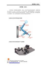
<str<strong>on</strong>g>adaptive</str<strong>on</strong>g> <str<strong>on</strong>g>optics</str<strong>on</strong>g> <str<strong>on</strong>g>system</str<strong>on</strong>g>. In this paper we discuss the performance of a <strong>LC</strong>-<strong>SLM</strong> in <str<strong>on</strong>g>open</str<strong>on</strong>g>-<str<strong>on</strong>g>loop</str<strong>on</strong>g>correcti<strong>on</strong>.2. Experimental setup and theoryUsually the residual wavefr<strong>on</strong>t error after correcti<strong>on</strong> is used to evaluate the correcti<strong>on</strong><str<strong>on</strong>g>precisi<strong>on</strong></str<strong>on</strong>g> for the closed-<str<strong>on</strong>g>loop</str<strong>on</strong>g> <str<strong>on</strong>g>adaptive</str<strong>on</strong>g> <str<strong>on</strong>g>optics</str<strong>on</strong>g> <str<strong>on</strong>g>system</str<strong>on</strong>g>. But the residual wavefr<strong>on</strong>t error couldnot be measured in the <str<strong>on</strong>g>open</str<strong>on</strong>g>-<str<strong>on</strong>g>loop</str<strong>on</strong>g> <str<strong>on</strong>g>adaptive</str<strong>on</strong>g> <str<strong>on</strong>g>system</str<strong>on</strong>g> [Fig. 1(b)], so we try to use the <str<strong>on</strong>g>open</str<strong>on</strong>g>-<str<strong>on</strong>g>loop</str<strong>on</strong>g>c<strong>on</strong>trol method <strong>on</strong> the closed-<str<strong>on</strong>g>loop</str<strong>on</strong>g> optical <str<strong>on</strong>g>system</str<strong>on</strong>g>. With this method, <str<strong>on</strong>g>open</str<strong>on</strong>g>-<str<strong>on</strong>g>loop</str<strong>on</strong>g> correcti<strong>on</strong> isprocessed, and the correcti<strong>on</strong> performance, especially the correcti<strong>on</strong> <str<strong>on</strong>g>precisi<strong>on</strong></str<strong>on</strong>g>, can also betested. The closed-<str<strong>on</strong>g>loop</str<strong>on</strong>g> optical c<strong>on</strong>figurati<strong>on</strong> is shown in Fig. 2.Fig. 2. Layout of the optical <str<strong>on</strong>g>system</str<strong>on</strong>g>.The <strong>LC</strong>-<strong>SLM</strong> used in the <str<strong>on</strong>g>system</str<strong>on</strong>g> is a liquid crystal <strong>on</strong> silic<strong>on</strong> (<strong>LC</strong>OS) device produced byBNS Company, and the wavefr<strong>on</strong>t sensor is the Shack-Hartmann wavefr<strong>on</strong>t sensor (WFS)HASO-32. The light source is a fiber bundle with white light output (MF). The bundle’sdiameter is 1 mm and its core diameter is 0.025 mm. Due to the chromatic dispersi<strong>on</strong> of liquidcrystal, the phase modulati<strong>on</strong> for different colors of light is different, so a color filter (CF,center wavelength of 633 nm and bandwidth of 10 nm) is used to make the light nearlym<strong>on</strong>ocolor. A rotatable polarizer (P) is used to polarize the light matching with the <strong>LC</strong>OS. Atthe positi<strong>on</strong> of Ab-L, which is c<strong>on</strong>jugated with the <strong>LC</strong>OS, several different aberrati<strong>on</strong> lensescan be inserted respectively to induce additi<strong>on</strong>al aberrati<strong>on</strong>. Behind the corrector <strong>LC</strong>OS anormal beam splitter is used to split the beam into two parts. One half goes into the imagingcamera to form the image, and the other half goes into the WFS (HASO) to measure theresidual error. The HASO is also c<strong>on</strong>jugated with the <strong>LC</strong>OS. The parameters of the HASOand <strong>LC</strong>OS are listed in Table 1, and the angle between the incident light and the reflectedlight from the <strong>LC</strong>OS is 5 deg, so the light is near-normally illuminated. What’s more, the halffield-of-view angel for the pupil image plane of the <strong>LC</strong>OS is 0.5 deg.Table. 1. Detailed parameters for the HASO-32 and BNS <strong>LC</strong>OSHASO-32BNS <strong>LC</strong>OSAperture dimensi<strong>on</strong> 4.9 x 4.9 mm Array size 7.68 x 7.68 mmSubaperture number 32 x 32 Active pixels 512 x 512Measurement accuracyin relative mode1/150 λ (RMS)Phase levels( resolvable )50 linear levels for 2πphase strokerepeatability
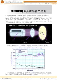
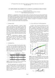
In the typical closed-<str<strong>on</strong>g>loop</str<strong>on</strong>g> c<strong>on</strong>trol <str<strong>on</strong>g>system</str<strong>on</strong>g>, the phase generated by the <strong>LC</strong>OS can beexpressed asΦ = Φ − k ⋅Φ ,i i−1i<strong>LC</strong>OS <strong>LC</strong>OS WFSwhere Ф WFS is the wavefr<strong>on</strong>t tested by the WFS, i is the number of iterati<strong>on</strong>s for theclosed-<str<strong>on</strong>g>loop</str<strong>on</strong>g>, and k is the closed-<str<strong>on</strong>g>loop</str<strong>on</strong>g> proporti<strong>on</strong> factor varying from 0 to 1. In order to process<str<strong>on</strong>g>open</str<strong>on</strong>g>-<str<strong>on</strong>g>loop</str<strong>on</strong>g> <str<strong>on</strong>g>adaptive</str<strong>on</strong>g> correcti<strong>on</strong> and measure the residual wavefr<strong>on</strong>t error after correcti<strong>on</strong>, weuse <str<strong>on</strong>g>open</str<strong>on</strong>g>-<str<strong>on</strong>g>loop</str<strong>on</strong>g> c<strong>on</strong>trol theory <strong>on</strong> the closed-<str<strong>on</strong>g>loop</str<strong>on</strong>g> optical setup as follows:StartMeasure the <str<strong>on</strong>g>system</str<strong>on</strong>g> wavefr<strong>on</strong>taberrati<strong>on</strong> Ф WFSSend gray map to <strong>LC</strong>OS to generatewavefr<strong>on</strong>t Ф <strong>LC</strong>OS =-Ф WFSClean the graymap <strong>on</strong> <strong>LC</strong>OSHold the gray map <strong>on</strong> <strong>LC</strong>OS and measurethe residual wavefr<strong>on</strong>t error σIt should be emphasized that the <str<strong>on</strong>g>system</str<strong>on</strong>g>atic wavefr<strong>on</strong>t aberrati<strong>on</strong> is almost static becausethe optical <str<strong>on</strong>g>system</str<strong>on</strong>g> is indoor and compact. Figure 3 shows the wavefr<strong>on</strong>t aberrati<strong>on</strong> with the<str<strong>on</strong>g>system</str<strong>on</strong>g> aberrati<strong>on</strong> (background) subtracted. The curve in Fig. 3 indicates that the fluctuati<strong>on</strong>of the aberrati<strong>on</strong> is smaller than 0.01λ (RMS) in 5 min; therefore the residual wavefr<strong>on</strong>t errorσ tested in the third step of the correcti<strong>on</strong> <str<strong>on</strong>g>loop</str<strong>on</strong>g> can be c<strong>on</strong>sidered as the correcti<strong>on</strong> error.Fig. 3. Wavefr<strong>on</strong>t error measured in relative mode for 5 min.3. Repeatability and linearity of the <strong>LC</strong>-<strong>SLM</strong>In the pure <str<strong>on</strong>g>open</str<strong>on</strong>g>-<str<strong>on</strong>g>loop</str<strong>on</strong>g> <str<strong>on</strong>g>adaptive</str<strong>on</strong>g> <str<strong>on</strong>g>optics</str<strong>on</strong>g> <str<strong>on</strong>g>system</str<strong>on</strong>g>, high <str<strong>on</strong>g>precisi<strong>on</strong></str<strong>on</strong>g> of <strong>on</strong>ly <strong>on</strong>e time correcti<strong>on</strong> isnecessary, because the residual error after correcti<strong>on</strong> cannot be detected and recorrected. As aresult high wavefr<strong>on</strong>t measurement <str<strong>on</strong>g>precisi<strong>on</strong></str<strong>on</strong>g> for the WFS and high wavefr<strong>on</strong>t rec<strong>on</strong>structi<strong>on</strong><str<strong>on</strong>g>precisi<strong>on</strong></str<strong>on</strong>g> for the corrector <strong>LC</strong>-<strong>SLM</strong> are necessary. Good repeatability and linearity of the<strong>LC</strong>-<strong>SLM</strong> are two key factors to achieve high wavefr<strong>on</strong>t rec<strong>on</strong>structi<strong>on</strong> <str<strong>on</strong>g>precisi<strong>on</strong></str<strong>on</strong>g>. Due to thehigh <str<strong>on</strong>g>precisi<strong>on</strong></str<strong>on</strong>g> of the WFS HASO-32 (1/150λ in relative mode), we use it to test the wavefr<strong>on</strong>trec<strong>on</strong>structi<strong>on</strong> <str<strong>on</strong>g>precisi<strong>on</strong></str<strong>on</strong>g> of the <strong>LC</strong>-<strong>SLM</strong> BNS <strong>LC</strong>OS first.The c<strong>on</strong>trol of the <strong>LC</strong>OS is <str<strong>on</strong>g>based</str<strong>on</strong>g> <strong>on</strong> Zernike polynomials [17], so the <str<strong>on</strong>g>precisi<strong>on</strong></str<strong>on</strong>g> ofwavefr<strong>on</strong>t generati<strong>on</strong> for <strong>on</strong>ly <strong>on</strong>e Zernike polynomial is tested at first. Figure 4 shows thegray map sent <strong>on</strong> the <strong>LC</strong>OS and the wavefr<strong>on</strong>t map measured by the WFS when Z 3 =1 (pist<strong>on</strong>is obviated; Z 0 , x-tilt; Z 1 , y-tilt; Z 2 , defocus, Z 3 , astigmatism; … Z 35 . Without remark, Z m =jmeans the mth Zernike coefficient is set to j and the other coefficients are set to 0). Figure 5#105446 - $15.00 USD Received 23 Dec 2008; revised 22 Mar 2009; accepted 24 Mar 2009; published 12 Jun 2009(C) 2009 OSA 22 June 2009 / Vol. 17, No. 13 / OPTICS EXPRESS 10777
shows the Zernike coefficients of the rec<strong>on</strong>structed wavefr<strong>on</strong>t measured by the WFS whenZ 2 =2, Z 3 =-2, and Z 5 =1. Many more test results are listed in Table 2. The maximum wavefr<strong>on</strong>trec<strong>on</strong>structi<strong>on</strong> error for the 24 Zernike modals is <strong>on</strong>ly 0.046λ RMS.(a) Gray map sent <strong>on</strong> <strong>LC</strong>OS(b) Wavefr<strong>on</strong>t measured by WFSFig. 4. Wavefr<strong>on</strong>t rec<strong>on</strong>structi<strong>on</strong> test for Z 3=1.ZernikeorderTable. 2. Wavefr<strong>on</strong>t rec<strong>on</strong>structi<strong>on</strong> error for Z 4 - Z 24Rec<strong>on</strong>structi<strong>on</strong>error (RMS)ZernikeorderRec<strong>on</strong>structi<strong>on</strong>error (RMS)ZernikeorderRec<strong>on</strong>structi<strong>on</strong>error (RMS)Z 4 =2 0.034λ Z 11 =1 0.033λ Z 18 =-2 0.042λZ 5 =1 0.028λ Z 12 =2 0.041λ Z 19 =1 0.031λZ 6 =-1 0.030λ Z 13 =2 0.037λ Z 20 =1 0.034λZ 7 =-2 0.041λ Z 14 =1 0.034λ Z 21 =2 0.038λZ 8 =2 0.035λ Z 15 =-1 0.029λ Z 22 =-1 0.031λZ 9 =2 0.046λ Z 16 =-1 0.032λ Z 23 =-1 0.035λZ 10 =1 0.038λ Z 17 =2 0.045λ Z 24 =2 0.043λFig. 5. Zernike coefficient tested by the WFS when the <strong>LC</strong>OS gray map is Z 2=2, Z n=0; Z 3= -2,Z n=0; and Z 5=1, Z n=0. The rec<strong>on</strong>structi<strong>on</strong> wavefr<strong>on</strong>t error (RMS) is 0.038λ, 0.031λ, and0.027λ, respectively.The linearity for <strong>LC</strong>OS wavefr<strong>on</strong>t generati<strong>on</strong> is tested for <strong>on</strong>ly Z 2 –Z 7 . Take Z 2 forexample; first Z n (n=0 … 35 and n≠2) is set to 0, then Z 2 is set from –3 to 3 in turn, and therec<strong>on</strong>structed wavefr<strong>on</strong>t is measured by the HASO. The results for the linearity test are shown#105446 - $15.00 USD Received 23 Dec 2008; revised 22 Mar 2009; accepted 24 Mar 2009; published 12 Jun 2009(C) 2009 OSA 22 June 2009 / Vol. 17, No. 13 / OPTICS EXPRESS 10778
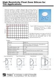
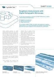
in Fig. 6(a). The maximum absolute deviati<strong>on</strong> between the measured Zernike coefficients andthe ideal is 0.072, and the maximum relative deviati<strong>on</strong> (normalized by the value of thecoefficient) is 5.1%.The repeatability of the <strong>LC</strong>OS is tested by this method: the gray map for Z m =j is sent to the<strong>LC</strong>OS and cleared repeatedly at 0.25 Hz; the wavefr<strong>on</strong>t is tested at 10 Hz simultaneously andthe Zernike coefficients of the wavefr<strong>on</strong>t are saved. The repeatability test results for Z 2 –Z 7 areshown in Fig. 6(b). The deviati<strong>on</strong>s for Z 2 –Z 7 are ±0.026, ±0.043, ±0.032, ±0.039, ±0.045, and±0.051. Thus the maximum repeatability error is 3.2% relatively.(a) Linearity test for <strong>LC</strong>OS.(b) Repeatability test for <strong>LC</strong>OS.Fig. 6. (a) Linearity and (b) repeatability tests for the <strong>LC</strong>OS.As the maximum relative errors for linearity and repeatability are 5.1% and 3.2%,respectively, the maximum possible residual error after correcti<strong>on</strong> will be 5%–8% comparedwith the initial wavefr<strong>on</strong>t error. If the initial wavefr<strong>on</strong>t error is 1.5λ (RMS), after <str<strong>on</strong>g>open</str<strong>on</strong>g>-<str<strong>on</strong>g>loop</str<strong>on</strong>g>correcti<strong>on</strong> there will be 0.075–0.12λ (RMS) residual error, which can improve the Strehl ratioto 0.57–0.8 at least.4. Open-<str<strong>on</strong>g>loop</str<strong>on</strong>g> correcti<strong>on</strong> resultThe initial <str<strong>on</strong>g>system</str<strong>on</strong>g> wavefr<strong>on</strong>t aberrati<strong>on</strong> without any aberrati<strong>on</strong> lens inserted at the positi<strong>on</strong>Ab-L is about 0.213λ (RMS), and the main comp<strong>on</strong>ent of the aberrati<strong>on</strong> is astigmatism, whichcan be seen from the wavefr<strong>on</strong>t map L0 in Fig. 7(a). After correcti<strong>on</strong> the residual wavefr<strong>on</strong>taberrati<strong>on</strong> is nearly 0.04λ (RMS). Then different eyepieces (myopia eyepiece and astigmatismeyepiece) used as the aberrati<strong>on</strong> lens are inserted into the positi<strong>on</strong> Ab-L to induce largeraberrati<strong>on</strong>. The wavefr<strong>on</strong>t maps after the aberrati<strong>on</strong> lens is inserted are shown in Fig. 7(a).Figure 7(b) shows the residual wavefr<strong>on</strong>t maps after <str<strong>on</strong>g>open</str<strong>on</strong>g>-<str<strong>on</strong>g>loop</str<strong>on</strong>g> correcti<strong>on</strong>. As the initialaberrati<strong>on</strong> increases, the residual aberrati<strong>on</strong> after correcti<strong>on</strong> increases too. But the residualwavefr<strong>on</strong>t error is still smaller than 0.08λ (RMS) even if the initial aberrati<strong>on</strong> is larger than2.5λ (RMS). The peak-to-valley (PV) values of the initial wavefr<strong>on</strong>t aberrati<strong>on</strong> with L3 andL4 inserted are 9.82λ and 10.13λ, respectively. Simultaneously the image of the fiber bundleis grabbed by the camera, so that we can judge the <str<strong>on</strong>g>open</str<strong>on</strong>g>-<str<strong>on</strong>g>loop</str<strong>on</strong>g> correcti<strong>on</strong> effect from the imageintuitively. It should be emphasized that the ideal resoluti<strong>on</strong> at the object space for this optical<str<strong>on</strong>g>system</str<strong>on</strong>g> is 21.5 µm, and the core diameter of the fiber bundle is 25 µm.#105446 - $15.00 USD Received 23 Dec 2008; revised 22 Mar 2009; accepted 24 Mar 2009; published 12 Jun 2009(C) 2009 OSA 22 June 2009 / Vol. 17, No. 13 / OPTICS EXPRESS 10779
L0:RMS 0.213λ L1:RMS 0.912λ L2:RMS 1.893λ L3:RMS 2.678λ L4: RMS 2.512λ(a) The initial wavefr<strong>on</strong>t mapL0:RMS 0.043λ L1:RMS 0.052λ L2:RMS 0.065λ L3:RMS 0.079λ L4: RMS 0.077λ(b) The residual wavefr<strong>on</strong>t aberrati<strong>on</strong> after <str<strong>on</strong>g>open</str<strong>on</strong>g>-<str<strong>on</strong>g>loop</str<strong>on</strong>g> correcti<strong>on</strong>Fig. 7. Wavefr<strong>on</strong>t map for different aberrati<strong>on</strong> lenses inserted. L0 means no lens inserted, L1means lens 1 inserted, L2 means lens 2 inserted, and so <strong>on</strong>. L1–L3 are myopia eyepieces andL4 is the astigmatism eyepiece.(a) The initial fiber images after aberrati<strong>on</strong> lens inserted(b) The fiber images after aberrati<strong>on</strong> correctedFig. 8. The fiber images before and after wavefr<strong>on</strong>t aberrati<strong>on</strong> is corrected. The order for theimages is the same as in Fig. 7: from left to right L0 (no lens inserted), L1, … , L4 in turn.In additi<strong>on</strong>, the stability is also very important for an <str<strong>on</strong>g>adaptive</str<strong>on</strong>g> <str<strong>on</strong>g>system</str<strong>on</strong>g>, so the <str<strong>on</strong>g>open</str<strong>on</strong>g>-<str<strong>on</strong>g>loop</str<strong>on</strong>g>correcti<strong>on</strong> is repeated for more than 100 cycles for every case (L0–L4) in order to test itsstability. The RMS value of the wavefr<strong>on</strong>t is calculated during the whole correcti<strong>on</strong> process.Figure 9 shows the RMS value of the wavefr<strong>on</strong>t for six cycles when lens 2 is inserted and lens4 is inserted. In each cycle, the wavefr<strong>on</strong>t is measured two times before correcti<strong>on</strong> and ninetimes after correcti<strong>on</strong> repeatedly. The residual errors after correcti<strong>on</strong> vary from 0.060λ to0.067λ (RMS) during the whole correcti<strong>on</strong> process for the case of lens 2 inserted, and theresidual errors after correcti<strong>on</strong> vary from 0.071λ to 0.079λ (RMS) for the case of lens 4inserted. It can be c<strong>on</strong>cluded from the experimental results that the repeatability <str<strong>on</strong>g>precisi<strong>on</strong></str<strong>on</strong>g> ofthe <str<strong>on</strong>g>open</str<strong>on</strong>g>-<str<strong>on</strong>g>loop</str<strong>on</strong>g> correcti<strong>on</strong> is 0.01λ (RMS).#105446 - $15.00 USD Received 23 Dec 2008; revised 22 Mar 2009; accepted 24 Mar 2009; published 12 Jun 2009(C) 2009 OSA 22 June 2009 / Vol. 17, No. 13 / OPTICS EXPRESS 10780
(a) Wavefr<strong>on</strong>t RMS with lens 2 inserted(b) Wavefr<strong>on</strong>t RMS with lens 4 inserted5. C<strong>on</strong>clusi<strong>on</strong>Fig. 9. Wavefr<strong>on</strong>t RMS during <str<strong>on</strong>g>open</str<strong>on</strong>g>-<str<strong>on</strong>g>loop</str<strong>on</strong>g> correcti<strong>on</strong> for about six cycles.A closed-<str<strong>on</strong>g>loop</str<strong>on</strong>g> <str<strong>on</strong>g>adaptive</str<strong>on</strong>g> optical <str<strong>on</strong>g>system</str<strong>on</strong>g> with a Shack-Hartmann wavefr<strong>on</strong>t sensor (HASO-32)and a <strong>LC</strong>-<strong>SLM</strong> (BNS <strong>LC</strong>OS) has been c<strong>on</strong>structed <str<strong>on</strong>g>based</str<strong>on</strong>g> <strong>on</strong> the theory of <str<strong>on</strong>g>open</str<strong>on</strong>g>-<str<strong>on</strong>g>loop</str<strong>on</strong>g>correcti<strong>on</strong>. With this method, <str<strong>on</strong>g>open</str<strong>on</strong>g>-<str<strong>on</strong>g>loop</str<strong>on</strong>g> correcti<strong>on</strong> was carried out and the correcti<strong>on</strong><str<strong>on</strong>g>precisi<strong>on</strong></str<strong>on</strong>g> was tested. The repeatability and linearity of the <strong>LC</strong>OS was tested first. Itsrepeatability error is 3.2% relatively and its linearity deviati<strong>on</strong> is about 5%. In the <str<strong>on</strong>g>open</str<strong>on</strong>g>-<str<strong>on</strong>g>loop</str<strong>on</strong>g>correcti<strong>on</strong> with the <strong>LC</strong>OS, the residual error after correcti<strong>on</strong> could reach 0.07λ (RMS) whenthe initial wavefr<strong>on</strong>t aberrati<strong>on</strong> was below 2λ (RMS), and even if the initial wavefr<strong>on</strong>taberrati<strong>on</strong> were larger than 2.5λ (RMS), the residual error after correcti<strong>on</strong> could reach 0.08λ(RMS). The repeatability <str<strong>on</strong>g>precisi<strong>on</strong></str<strong>on</strong>g> of the <str<strong>on</strong>g>open</str<strong>on</strong>g>-<str<strong>on</strong>g>loop</str<strong>on</strong>g> correcti<strong>on</strong> is 0.01λ (RMS) for the indooroptical <str<strong>on</strong>g>system</str<strong>on</strong>g>. Besides, by using an <str<strong>on</strong>g>open</str<strong>on</strong>g>-<str<strong>on</strong>g>loop</str<strong>on</strong>g> optical <str<strong>on</strong>g>system</str<strong>on</strong>g> the light energy efficiency forthe <strong>LC</strong>-<strong>SLM</strong> and the <str<strong>on</strong>g>system</str<strong>on</strong>g> bandwidth could be improved.Although a <strong>LC</strong>-<strong>SLM</strong> has been used for atmospheric turbulence compensati<strong>on</strong> [15,16], theloss of light energy due to the polarizati<strong>on</strong> requirement and the slow resp<strong>on</strong>se of liquid crystalare the two critical drawbacks. Thus it can be expected that <str<strong>on</strong>g>open</str<strong>on</strong>g>-<str<strong>on</strong>g>loop</str<strong>on</strong>g> correcti<strong>on</strong> can improvethe performance of a <strong>LC</strong>-<strong>SLM</strong> for atmospheric turbulence compensati<strong>on</strong> significantly.Besides, the increase of light efficiency will be very beneficial for using a <strong>LC</strong>-<strong>SLM</strong> in humaneye aberrati<strong>on</strong> correcti<strong>on</strong>. As the light efficiency increases, the light energy used to illuminatethe retina can be reduced, which is much safer for the human eye.AcknowledgmentsThis work was supported by Nati<strong>on</strong>al Natural Science Foundati<strong>on</strong> (No. 60578035, No.50473040, and No. 60736042) and the Science Foundati<strong>on</strong> of Jilin Province (No. 20050520and No. 20050321-2).#105446 - $15.00 USD Received 23 Dec 2008; revised 22 Mar 2009; accepted 24 Mar 2009; published 12 Jun 2009(C) 2009 OSA 22 June 2009 / Vol. 17, No. 13 / OPTICS EXPRESS 10781