A Tabu Search Heuristic Based on k-Diamonds for ... - ePrints Soton

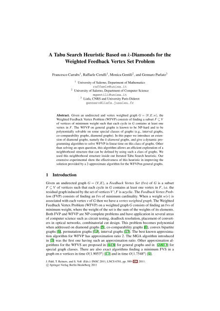
A <strong>Tabu</strong> <strong>Search</strong> <strong>Heuristic</strong> <strong>Based</strong> on k-Diamonds for theWeighted Feedback Vertex Set ProblemFrancesco Carrabs 1 , Raffaele Cerulli 1 , Monica Gentili 2 , and Gennaro Parlato 31 University of Salerno, Department of Mathematicsraffaele@unisa.it2 University of Salerno, Department of Computer Sciencemgentili@unisa.it3 Liafa, CNRS and University Paris Diderotgennaro@liafa.jussieu.frAbstract. Given an undirected and vertex weighted graph G =(V,E,w), theWeighted Feedback Vertex Problem (WFVP) consists of finding a subset F ⊆ Vof vertices of minimum weight such that each cycle in G contains at least onevertex in F. The WFVP on general graphs is known to be NP-hard and to bepolynomially solvable on some special classes of graphs (e.g., interval graphs,co-comparability graphs, diamond graphs). In this paper we introduce an extensionof diamond graphs, namely the k-diamond graphs, and give a dynamic programmingalgorithm to solve WFVP in linear time on this class of graphs. Otherthan solving an open question, this algorithm allows an efficient exploration of aneighborhood structure that can be defined by using such a class of graphs. Weused this neighborhood structure inside our Iterated <strong>Tabu</strong> <strong>Search</strong> heuristic. Ourextensive experimental show the effectiveness of this heuristic in improving thesolution provided by a 2-approximate algorithm for the WFVPon general graphs.1 IntroductionGiven an undirected graph G =(V,E), aFeedback Vertex Set (fvs) of G is a subsetF ⊆ V of vertices such that each cycle in G contains at least one vertex in F, i.e.theresidual graph induced by the set of vertices V \F is acyclic. The Feedback Vertex Problem(FVP) consists of finding an fvs of minimum cardinality. When a weight w(v) isassociated with each vertex v of G then we have a vertex weighted graph. The WeightedFeedback Vertex Problem (WFVP) on a weighted graph G consists of finding an fvs ofminimum weight, where the weight of the set is the sum of the weights of its elements.Both FVP and WFVP are NP-complete problems and have application in several areasof computer science such as circuit testing, deadlock resolution, placement of convertersin optical networks, combinatorial cut design. This problem becomes polynomialwhen addressed on diamond graphs [5], co-comparability graphs [6], convex bipartitegraphs [6], permutation graphs [14], interval graphs [15]. The best known approximationalgorithm for WFVP has approximation ratio 2. The MGA algorithm introducedin [3] was the first one having such an approximation ratio. Other approximation algorithmsfor the WFVS are proposed in [1,18] for general graphs and in [2,8,13] forspecial graph classes. There are also exact algorithms finding a minimum FVS in agraph on n vertices in time O(1.9053 n ) [17] and in time O(1.7548 n ) [9].J. Pahl, T. Reiners, and S. Voß (Eds.): INOC 2011, LNCS 6701, pp. 589–602, 2011.c○ Springer-Verlag Berlin Heidelberg 2011

590 F. Carrabs et al.In this paper we focus on the weighted feedback vertex set problem (WFVP). In particular,we introduce an extension of diamond graphs, namely the k-diamond graphs,and give a linear time algorithm to solve WFVP on it based on a dynamic programmingapproach. Moreover, we show how this new class of graphs can be used to definea neighborhood structure (namely, the k-diamond Neighborhood) of a given feasiblesolution and, successively, we show how to solve the problem on general graphs bymeans of a tabu search technique using the k-diamond neighborhood. Such a classof neighborhood was already introduced in [4], where, however, the computationalcomplexity of finding an optimum WFVP on a k-diamond graph was left open anda heuristic approach was used to solve the problem. We solve such an open problem(by giving a linear time algorithm) and also show the effectiveness of the chosen neighborhoodin improving a given initial feasible solution when explored by means of ourexploration strategy. In order to do this, experimental results are given to show howour Iterative <strong>Tabu</strong> <strong>Search</strong> can improve the initial feasible solution, returned by the 2-approximate MGA algorithm [3], when the k-diamond neighborhood is defined and efficientlyexplored.The sequel of the paper is organized as follows. Section 2 introduces the basic notation.Section 3 describes the class of k-diamond graphs and contains the main propertiesto solve WFVP in linear time on this class. The role of k-diamonds to define a neighborhoodstructure is described in Section 4, together with the proposed Iterated <strong>Tabu</strong><strong>Search</strong> heuristic. Computational results are reported in Section 5. Finally, concludingremarks are discussed in Section 6.2 Definitions and NotationLet G =(V,E,w) be an undirected and vertex weighted graph, where V is the set of nvertices, E is the set of m edges, and, w(v) is a positive weight associated with eachvertex v ∈ V. Given a subset X ⊆ V of vertices, let us define its weight W(X) as the sumof the weights of its elements, i.e. W(X)=∑ v∈X w(v) and ¯X = V \ X its complementaryset. If X = /0 thenW(X)=0. We denote by G[X] the subgraph of G induced by the setof vertices X ⊆ V . Formally, G[X]=(X,E [X] ,w) where E [X] = {(x,y) ∈ E : x,y ∈ X}.Atree T r rooted in r is an acyclic and connected graph. We define a forest F as a graphwhere any connected component is a tree. A subset of vertices X is a feedback vertexset of G if and only if G[ ¯X] is a forest. From now on we denote by F(G) and F ∗ (G),any feedback vertex set and the minimum weight feedback vertex set of G, respectively.When no confusion may arise we simply denote these sets by F and F ∗ respectively.Moreover, we define F¯v a feedback vertex set of G not containing vertex v. Avertexv ∈ F is redundant if and only if F \{v} is a feedback vertex set of G.Anyvertexv ∈ Vis said to be appended if it is not included in any cycle of G. Obviously, a set of verticesis an fvs of G if and only if it is an fvs of the graph G ′ obtained from G after deletingall the appended vertices. We say a graph is reduced if it does not contain any appendedvertex. The reduction operation of a graph can be performed in linear time. W.l.o.g.,from now on we suppose graph G to be a reduced graph. For any additional definitionand notation we refer to [7].

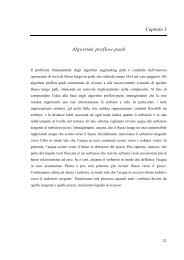
<strong>Tabu</strong> <strong>Search</strong> to Solve the Weighted Feedback Vertex Set Problem 59111814232 3 491015 1645 65 6 7 11 12 1317 187 8 91019(a)(b)Fig. 1. (a) A diamond with upper apex r = 1 and lower apex z = 10. (b)A3-diamond with upperapices R = {1,8,14} and lower apex z = 19. Note that, as stated by property 1, it is composed bythe three diamonds D 1 ,D 8 and D 14 .3 The Classofk-Diamond GraphsIn this section we first recall the definition of the class of diamond graphs introducedin [5], and successively we formally describe the extended class of k-diamond graphs.Then, we prove the basic properties that are useful to optimally solve WFVP on thisnew class in linear time.A weighted diamond D r,z =(V r ,E r ,w) is an undirected and vertex weighted graphwhere (i) each vertex v ∈ V r is included in at least one simple path between r and z and(ii) D r,z [¯z] is a tree. The two vertices r and z are called the upper and lower apex of adiamond D r,z , respectively, and, the subgraph D r,z [¯z] is referred to as the tree T r rooted inr associated with D r,z . In Figure 1(a) the diamond D 1,10 with upper apex r = 1andlowerapex z = 10 is shown. Note that by deleting vertex z we obtain the tree T 1 = D 1,10 [ 10]. ¯As shown in [5], WFVP can be solved in linear time on a diamond graph by a dynamicprogramming algorithm. Let us refer to such an algorithm as DP. In the sequelwe show how to use DP to solve WFVP in linear time on a k-diamond. A k-diamond isa generalization of a diamond where multiple upper apices are allowed, formally:Definition 1. A weighted k-diamond D R,z =(V R ,E R ,w), wherek≥ 1,R= {r 1 ,r 2 ,...,r k }⊆V R and z ∈ V R , is an undirected and vertex weighted graph where (i) each vertexv ∈ V R is included in a simple path between exactly one of the k apices r i ∈ R and z and(ii) D R,z [¯z] is a forest with k connected components.Following the definition introduced for diamond graphs, we refer to the set of vertices Rand to vertex z of D R,z as the set of upper apices and the lower apex of D R,z , respectively.The subgraph D R,z [¯z] is referred to as the forest F R , associated with D R,z , whose connectedcomponents are the k trees T ri rooted in r i ∈ R. Figure 1(b) shows a 3-diamond.The set of upper apices is composed of the three vertices R = {1,8,14}, while the lowerapex is vertex z = 19. The graph obtained from D R,z , after deleting the lower apex, is aforest with the three connected components T 1 , T 8 and T 14 . To keep notation simple, inthe sequel of the paper and when no confusion may arise, we denote a k-diamond D R,z ,

592 F. Carrabs et al.with R = {r 1 ,...,r k },justbyD R and a diamond graph D r,z by D r . Note that for k = 1ak-diamond is a diamond. Moreover, it is easy to see that the following property holds:Property 1 (Decomposition). Any k-diamond D R is composed by k distinct diamondsD ri , with r i ∈ R, having all the same lower apex z.For instance, the 3-diamond depicted in Figure 1(b) is composed by three diamondsD 1 , D 8 and D 14 . We will see in the following how to use the decomposition propertyto solve WFVP on D R . By definition of k-diamond, the following properties obviouslyhold.Property 2. The singleton {z} is an fvs of D R .Property 3. Every cycle of D R contains vertex z and vertices belonging to the sameconnected component of F R .Observe that, by property 2, a minimum weight feedback vertex set F ∗ (D R ) of D Reither contains vertex z or not. Therefore, to find F ∗ (D R ) we can proceed as follows:(i) compute the minimum weight feedback vertex set F ∗¯z (D R ) that does not containz; (ii) if W(F ∗¯z (D R)) < w(z) then set F ∗ (D R )=F ∗¯z (D R) otherwise set F ∗ (D R )={z}.The computation of F ∗¯z (D R) can be carried out by finding the fvs F ∗ (D Ri ) of minimumweight on each of the k diamonds D ri that compose D R as proven by the followinglemma:Lemma 1. Given the k-diamond D R ,letF ∗¯z (D ri ), ∀r i ∈ R, be a minimum weight feedbackvertex set of diamond D ri not containing vertex z. Then: F ∗¯z (D R)= ⋃F ∗¯z (D r i).Proof. Let X = ⋃ r i ∈R F ∗¯z (D r i). We need to prove that X is a minimum fvs of D R notcontaining z,i.e.X = F ∗¯z (D R ). From property 3 and by definition of F ∗¯z (D ri ), it is evidentthat X is an fvs of D R therefore we have only to prove that X is minimum. Let ussuppose, by contradiction, there exists another fvs, say Y, such that z /∈ Y and W(Y )

<strong>Tabu</strong> <strong>Search</strong> to Solve the Weighted Feedback Vertex Set Problem 593Procedure: DP multiStep 1. for all D ri compute Fz ∗(Dr i);Step 2. Set Fz ∗ (D R) ← ⋃Fz ∗ (D r i);r i ∈RStep 3. if W (Fz ∗(DR)) < w(z) then F ∗ (D R ) ← Fz ∗(DR) otherwise F ∗ (D R ) ←{z};Step 4. Return F ∗ (D R );Fig. 2. Pseudo code of algorithm DP multitotal cost of step 1 is equal to O(|V R |) time. The joining operation carried out at step 2requires O(k) time, while step 3 and step 4 require constant time. Consequently, DP multiruns in O(|V R |) time.⊓⊔The next sections contain a description of a general neighborhood structure based onthe class of k-diamonds and introduce an operator that, using DP multi , efficiently exploressuch a neighborhood. This operator will be later embedded into our Iterated<strong>Tabu</strong> <strong>Search</strong>.4 The Neighborhood Structures and the Iterative <strong>Tabu</strong> <strong>Search</strong>The basic paradigm of tabu search is to use information about the search history to guidelocal search approaches to overcome local optimality. <strong>Based</strong> on some sort of memorycertain moves may be forbidden, we say they are set tabu (and appropriate move attributesare put into a list, the so-called tabu list). The search may imply acceptancedeteriorating moves when no improving moves exist or all improving moves of thecurrent neighborhood are set tabu. We implemented an extension of the standard <strong>Tabu</strong><strong>Search</strong> [10,11,12] (TS), namely the Iterated <strong>Tabu</strong> <strong>Search</strong> [16] (ITS), whose central ideais based on the concept of intensification and diversification. The intensification phaseis focused in finding a better (locally optimal) solution in “surroundings”, i.e. neighborhood,of the current solution. The ITS method uses the classical TS to achieve such animprovement. The Diversification phase is used whenever the tabu memory indicatesthat one is trapped in a certain basin of attraction and then allows to escape from thecurrent local optimum and to move towards new regions in the solution space.In the following subsections the main components of the algorithm are described: (i)the neighborhood structures (namely, the k-diamond neighborhood and the 2-exchangeneighborhood),(ii) the corresponding exploration strategies (namely, the Single−Insertand the Double − Insert operators, respectively); (iii) the tabu list and (iv) the diversificationphase. The pseudo-code of our Iterative <strong>Tabu</strong> <strong>Search</strong> (ITS) is given in Fig. 5.4.1 The k-Diamond NeighborhoodGiven a graph G, letF be any not redundant fvs of G and F = G[ ¯F] the forest inducedby vertices not in F. By inserting a vertex z ∈ F in F a k-diamond D R is obtained. Let I z

594 F. Carrabs et al.be an fvs of D R not containing z, then the set F ′ = I z ∪{F \{z}} is a new fvs of G.Notethat, F ′ could contain redundant vertices. Let O z be the set of the redundant vertices ofF ′ . Note that, by construction of I z ,wehaveO z ⊆ F \{z}.Addz to O z and consider thevertex set F new = I z ∪{F \ O z }. F new is a not redundant fvs of G and: if W (I z ) < W (O z ),its weight is lower than the weight of F. Given a vertex z ∈ F, we define the couple(I z ,O z ) an exchange set of z, formally:Definition 2. Given a vertex z ∈ F, the couple (I z ,O z ),whereI z ⊆ V \ F, O z ⊆ F andz ∈ O z , is a exchange set of z if the set I z ∪{F \ O z } is a not redundant fvs of G.Let us denote by E (F,z) the collection of all the exchange sets associated with z ∈F, i.e.E (F,z) = { (I z ,O z ) : I z ∪{F \ O z } is a not reduntant fvs of G } .Thek-diamondneighborhood is defined as follows:Definition 3. Given a graph G and an fvs F, the k-diamond neighborhood N (F) isthe set of all not redundant fvs of G that can be obtained from F through the exchangesets associated with each vertex z ∈ F:{}N (F)= I z ∪{F \ O z } : (I z ,O z ) ∈ E (F,z),∀z ∈ FNote that, given a vertex z ∈ F, finding the minimum cost set I z associated with it correspondsto find the minimum weight feedback vertex set on the k-diamond associatedwith z. Hence, by applying the DP multi algorithm we can perform an implicit exhaustiveexploration on the neighborhood to find a local optimum in polynomial time. Thisexploration is carried out by our first operator Single − Insert that is described next.The Single − Insert Operator Given a not redundant fvs F of G and the incumbentsolution F ∗ ,theSingle − Insert operator builds, for each z ∈ F, thek-diamondD R by introducing z in F = G[ ¯F]. Successively, it computes an exchange set (I z ,O z )where I z = F ∗¯z (D R), i.eI z is the minimum feedback vertex set of D R not containingz. The operator selects the best exchange set (I ∗ z ,O∗ z ) such that W(I∗ z ) − W(O∗ z )=min (Iz ,O z ):z∈F{W(I z ) − W(O z )}. More in detail (see Fig. 3), the operator builds the k-diamond D R (step 1), finds the fvs F ∗¯z (D R) by applying algorithm DP multi and setsI z ← F ∗¯z (D R) (step 2). The operator (step 3) finds redundant vertices (if any) of thenew fvs F new = F \{z}∪{I z } to be inserted in O z (initially O z = {z}). To this end,Single − Insert builds the forest F ′ = G[ ¯F new ] and reintroduces, one by one, each vertexz ′ ∈ F \{z} to check whether z ′ is redundant or not. If z ′ is redundant then it ismoved from F new to O z .ThefinalfvsF new = I z ∪{F \ O z } is then obtained after all thevertices in F \{z} are checked for redundancy. Note that the pair (I z ,O z ) is the movecorresponding to the transition from solution F to its neighbor F new .The weight of the new set F new is then compared with the weight of the incumbentsolution F ∗ found so far. If W(F new ) < W(F ∗ ), then the operator sets the best move(I ∗ z ,O ∗ z ) equal to (I z ,O z ) even if this move is tabu (this represents the application ofan aspiration criterion [12]). Otherwise, if (I z ,O z ) is not tabu and the correspondingsolution is better than the solution associated with (I ∗ z ,O ∗ z ), the algorithm sets (I ∗ z ,O ∗ z )equal to (I z ,O z ). Finally, if both previous cases do not hold, (I z ,O z ) is neglected.

<strong>Tabu</strong> <strong>Search</strong> to Solve the Weighted Feedback Vertex Set Problem 595Procedure: Single − Insert(G,F, F ∗ )Set W (I ∗ z ) ← ∞, W (O∗ z ) ← 0for all z ∈ F doStep 1. Insertz in G[ ¯F] and reduce the obtained graph to produce the k-diamond D R ;Step 2. SetI z ← F ∗¯z (D R);Step 3. Find the set of redundant nodes O z ,addz to O z ,andsetF new ← I z ∪{F \ O z };Step 4. if W (F new ) < W (F ∗ ) do // aspiration criterion //I ∗ z ← I z ,O ∗ z ← O z ;else if W (I z ) −W (O z ) < W(I ∗ z ) −W (O ∗ z ) and (I z ,O z ) is not tabu doI ∗ z ← I z,O ∗ z ← O z;end forreturn (I ∗ z ∪{F \ O∗ z }); Fig. 3. Pseudo-code of operator Single − Insert4.2 The 2-Exchange Neighborhood and the Double − Insert OperatorAdditional neighborhoods similar to the k-diamond neighborhood above described canbe considered if more than one vertex of F is selected to be introduced in F = G[ ¯F].Indeed, a drawback of the Single − Insert operator concerns the diversification of theexplored solutions. In fact, when there are not redundant vertices, only one vertex (thelower apex z) is moved from F to F = G[ ¯F]. Hence, in the worst case, several applicationsof the operator Single − Insert are necessary to remove more than one vertexfrom F. In order to overcome this issue, we consider a new neighborhood, namely the2-exchange neighborhood, to diversify the explored solutions, that is, we considered thecase when two vertices {z i ,z j } are selected to be inserted in F . This neighborhood isexplored by the operator Double − Insert (see Fig. 4) that differs from Single − Insertsince it inserts two lower apices {z i ,z j } into F , and finds the fvs I zi ,z jby applying algorithmMGA. MGA is a greedy algorithm that selects at each iteration the vertex v suchthat the ratio w(v)/d(v) is minimum, where d(v) is the degree of the vertex. When avertex is selected, it is removed from G and G is then reduced to obtain the subgraph G ′ .The degree of each vertex v in G ′ is updated and for each edge (u,v) that was removedduring the reduction process, the weight of its endpoints is decreased by the quantityw(v)/d(v). The selection of a new vertex is then carried out on G ′ until it is not empty.For more details on MGA the reader can refer to [3].The Single − Insert operator and the Double − Insert operator will be used duringthe intensification phase of Iterative <strong>Tabu</strong> <strong>Search</strong> metaheuristic.4.3 The <strong>Tabu</strong> ListAt iteration t, after a relocation of vertices is carried out according to a resulting exchangeset (I z ,O z ), the inverse move (O z ,I z ) cannot be carried out for the next Δ iterations,where Δ is the tabu list size. To implement a fast way for storing each move(O z ,I z ) we use a bit mask and an hash-table. Since both I z and O z are vertex sets andeach vertex has a distinct ID, we allocate two bit-mask bl and br whose size is |V|. Weset the bits in bl and br corresponding to the vertices in O z and I z , respectively, equal to

596 F. Carrabs et al.Procedure: Double − Insert(G,F,F ∗ )Set W (I ∗ C ) ← ∞, W (O∗ C ) ← 0for all pair C =(z i ,z j ) with z i ,z j ∈ F doStep 1. Insertz i and z j in G[ ¯F] and reduce it to obtain G ′ ;Step 2. ApplyMGAtofindanfvsI C of G ′ ;Step 3. Find the set of redundant nodes O C ,addz i and z j to O C and set F new ← I C ∪{F \O C };Step 4. if W (F new ) < W (F ∗ ) do // aspiration criterion //I ∗ C ← I C, O ∗ C ← O C;else if W (I C ) −W (O C ) < W (I ∗ C ) −W (O∗ C ) and (I C,O C ) is not tabu doI ∗ C ← I C, O ∗ C ← O C;end forreturn I ∗ C ∪{F \ O∗ C }; Fig. 4. Pseudo-code of operator Double − Insert1. The two strings are then concatenated to generate the string of bits bl-br, that is thekey associated with the move. This key, that is unique for each move, is given to the hashfunction to save the move. To verify if a move is tabu it is sufficient to generate its keyand check whether it is inside the hash table. The key generation, the insertion into thehash table and the checking operations require O(|I z | + |O z |) time. The keys are savedinside a FIFO queue whose size is Δ, hence when the queue is full and a new key hasto be inserted, the key on the head is removed from the queue and from the hash table.This operation requires constant time. We used a reactive tabu list, that uses a list whosesize is dynamically updated during the computation according to the evolution of thesearch. The value of Δ ranges between a lower bound β − and an upper bound β + thatare fixed at the beginning of the computation and never change. Given an initial fvs F,}and Δ = β − + (β + −β − )2. After each iterationwe set β − = 5, β + = max { 3β − , |F|3 , | ¯F|3t, if the new solution F ′ found during the intensification phase (steps 4-17 in Fig. 5) isbetter than F ∗ ,thenΔ is increased by one. Otherwise, if F ′ is worse than F ∗ but betterthan the solution found at the previous iteration then Δ is not changed. Finally, if F ′ isworse than the previous one then Δ is decreased by one.4.4 The Diversification PhaseThe diversification phase is implemented using a modified version of the Double −Insert operator (namely the Multi−Insert operator). Given a solution F, Multi−Insertdiffers from Double − Insert since a subset of vertices P ⊂ F with |P| > 2isinsertedinto the forest F = G[ ¯F] to obtain a new graph G ′ . There are three main aspects totake into account in the diversification phase: (i) when to apply the diversification andon which solution, (ii) the cardinality of the set P, and, (iii) which vertices to introducein P. We apply the diversification either to the best solution F ∗ found so far (step 23in Fig. 5) or to the solution F ′ (step 25 in Fig. 5) computed during the intensificationphase. We keep a counter q that ranges from 1 to θ (that is the maximum number ofdiversification operations performed by the algorithm) and, as soon as this bound isreached, the ITS stops. The cardinality of P is computed according to the following

<strong>Tabu</strong> <strong>Search</strong> to Solve the Weighted Feedback Vertex Set Problem 597Procedure: ITS(G,θ,σ)1: F ← F ∗ ← MGA(G);2: for q = 1toθ do3: // Intensification Phase4: F ′ ← V ;5: for h = 1toσ do6: F 1 ←Single-Insert(G,F,F ∗ );7: F 2 ←Double-Insert(G,F,F ∗ );8: if W (F 1 ) < W (F 2 ) then9: F ← F 1 ;10: else11: F ← F 2 ;12: end if13: Save the inverse move into the tabu list.14: if W (F) < W(F ′ ) then15: F ′ ← F; h ← 1;16: end if17: end for18: if W (F ′ ) < W (F ∗ ) then19: F ∗ ← F ′ ;20: end if21: // Diversification Phase22: if q is even then23: F ← Diversi f ication(F ∗ );24: else25: F ← Diversi f ication(F ′ );26: end if27: end for28: return F ∗ ;Fig. 5. Pseudo-code of Iterated <strong>Tabu</strong> <strong>Search</strong>formula: max { 5, |F|×(20+5q) }100 . Finally, to remove vertices from F we consider the lastiteration it + (v) when v has been inserted in F: the vertices of F are sorted in increasingorder according to it + (v) and the first |P| vertices of F are selected.5 Computational ResultsThe ITS algorithm was coded in C and run on a 2.33 GHz Intel Core2 Q8200 processor.Since there are no available benchmark instances for the WFVP, we generated instancesfor the following class of graphs: random graphs, squared and not squared grids, taurusand hypercube. Each instance is characterized by the number of vertices, the numberof edges, a seed and a range of values for the weight of the vertices. The weight rangesare: 10-25, 10-50 and 10-75. For each combination of parameters we generated fiveinstances with the same characteristics except for the seed. The results reported in thetables are average values over these five instances. Small instances have 25, 50 and 75vertices. Large instances have 100, 200, 300, 400 and 500 vertices.

598 F. Carrabs et al.Tables 1-2-3 report the results of the MGA algorithm and of our ITS algorithm. Thefirst and second columns in each table report the id and characteristics of each instance,respectively. For random graphs (Table 1): number of vertices (n), number of edges (m),the lower (low) and upper (up) bounds for the weight of each vertex. For the hypercubegraphs (Table 2a and 3a) the number of edges is omitted because it depends on thenumber of vertices. For the remaining graph classes: x is the number of rows and y is thenumber of columns. The third column in each table reports the solution value returnedTable 1. (a) Test results on random graphs: (a) small instances and (b) large instances(a)RANDOM GRAPHS: Small InstancesID Instance MGA ITS GAPn m low up Value Value Time1 25 33 10 25 70.8 63.8 0.00 -9.89%2 25 33 10 50 105.4 99.8 0.00 -5.31%3 25 33 10 75 133.6 125.2 0.00 -6.29%4 25 69 10 25 166.8 157.6 0.00 -5.52%5 25 69 10 50 294.8 272.2 0.00 -7.67%6 25 69 10 75 455 409.4 0.00 -10.02%7 25 204 10 25 286.4 273.4 0.02 -4.54%8 25 204 10 50 527 507 0.01 -3.80%9 25 204 10 75 829.8 785.8 0.01 -5.30%10 50 85 10 25 191.4 175.4 0.03 -8.36%11 50 85 10 50 298.2 280.8 0.03 -5.84%12 50 85 10 75 377.2 348 0.02 -7.74%13 50 232 10 25 409 389.4 0.07 -4.79%14 50 232 10 50 746.8 708.6 0.06 -5.12%15 50 232 10 75 1018.4 951.6 0.04 -6.56%16 50 784 10 25 612.6 602.2 0.11 -1.70%17 50 784 10 50 1204.2 1172.2 0.15 -2.66%18 50 784 10 75 1685.2 1649.4 0.14 -2.12%19 75 157 10 25 347.2 321 0.13 -7.55%20 75 157 10 50 571.2 526.2 0.14 -7.88%21 75 157 10 75 815 757.2 0.11 -7.09%22 75 490 10 25 654.2 638.6 0.16 -2.38%23 75 490 10 50 1286.6 1230.6 0.27 -4.35%24 75 490 10 75 1870.8 1793.6 0.13 -4.13%25 75 1739 10 25 903.2 891 0.40 -1.35%26 75 1739 10 50 1681 1664.8 0.35 -0.96%27 75 1739 10 75 2479.8 2452.8 0.33 -1.09%AVG -5.18%(b)RANDOM GRAPHS: Large InstancesID Instance MGA ITS GAPn m low up Value Value Time1 100 247 10 25 536.4 501.4 0.33 -6.52%2 100 247 10 50 910.4 845.8 0.37 -7.10%3 100 247 10 75 1279.2 1223.8 0.28 -4.33%4 100 841 10 25 846 828.2 0.27 -2.10%5 100 841 10 50 1793.2 1729.6 0.60 -3.55%6 100 841 10 75 2512.2 2425.6 0.35 -3.45%7 100 3069 10 25 1151.2 1134 0.59 -1.49%8 100 3069 10 50 2218 2179 0.69 -1.76%9 100 3069 10 75 3284 3228.8 0.77 -1.68%10 200 796 10 25 1547.8 1488.4 3.48 -3.84%11 200 796 10 50 2544.2 2442.6 2.50 -3.99%12 200 796 10 75 3277.4 3157 2.78 -3.67%13 200 3184 10 25 2035.6 2003.6 2.78 -1.57%14 200 3184 10 50 3775.2 3683.6 2.67 -2.43%15 200 3184 10 75 5259 5158.6 2.76 -1.91%16 200 12139 10 25 2467.4 2450 11.31 -0.71%17 200 12139 10 50 4182.2 4149.4 8.91 -0.78%18 200 12139 10 75 5568.8 5531.4 6.98 -0.67%19 300 1644 10 25 2136.6 2072.6 10.19 -3.00%20 300 1644 10 50 4384.6 4239.4 9.12 -3.31%21 300 1644 10 75 6411.2 6154.4 11.09 -4.01%22 300 7026 10 25 3267.6 3231 19.59 -1.12%23 300 7026 10 50 6368.4 6261.4 21.12 -1.68%24 300 7026 10 75 8825.2 8660.6 17.21 -1.87%25 300 27209 10 25 3749.2 3729.2 44.74 -0.53%26 300 27209 10 50 5774.2 5738 29.26 -0.63%27 300 27209 10 75 10514 10469.6 50.88 -0.42%28 400 2793 10 25 3097 3015.2 29.99 -2.64%29 400 2793 10 50 6726.8 6528 35.82 -2.96%30 400 2793 10 75 9006.8 8730 35.36 -3.07%31 400 12369 10 25 4514.4 4451.8 55.14 -1.39%32 400 12369 10 50 6896 6837.4 35.88 -0.85%33 400 12369 10 75 10788.8 10661.8 48.12 -1.18%34 400 48279 10 25 5090 5060.8 123.27 -0.57%35 400 48279 10 50 7142.6 7109.2 85.15 -0.47%36 400 48279 10 75 15202.4 15114.6 127.31 -0.58%37 500 4241 10 25 4197.4 4102.8 68.35 -2.25%38 500 4241 10 50 7447.6 7285 70.14 -2.18%39 500 4241 10 75 11619.6 11285.6 63.93 -2.87%40 500 19211 10 25 5817.2 5745.8 99.12 -1.23%41 500 19211 10 50 7819.2 7725 89.63 -1.20%42 500 19211 10 75 14335.4 14167.8 80.09 -1.17%43 500 75349 10 25 6388.6 6366.4 181.71 -0.35%44 500 75349 10 50 8709 8671.2 155.18 -0.43%45 500 75349 10 75 16994.6 16939.2 201.96 -0.33%AVG -2.09%

<strong>Tabu</strong> <strong>Search</strong> to Solve the Weighted Feedback Vertex Set Problem 599Table 2. (a) Test results on small instances:(a) hypercube graphs, (b) taurus graphs, (c) squaredgrid graphs and (d) not squared grid graphs(a)HYPERCUBE GRAPHS: Small InstancesID Instance MGA ITS GAPnlowupValue Value Time1 16 10 25 77.4 72.2 0.00 -6.72%2 16 10 50 99.8 93.8 0.00 -6.01%3 16 10 75 99.8 97.4 0.00 -2.40%4 32 10 25 177.2 170 0.01 -4.06%5 32 10 50 249.4 241 0.00 -3.37%6 32 10 75 286.2 277.6 0.00 -3.00%7 64 10 25 377.6 354.6 0.13 -6.09%8 64 10 50 486.2 476 0.05 -2.10%9 64 10 75 514 503.8 0.05 -1.98%AVG -3.97%(c)SQUARED GRID GRAPHS: Small InstancesID Instance MGA ITS GAPxylowup Value Value Time1 5 5 10 25 122.4 114 0.00 -6.86%2 5 5 10 50 208.4 199.8 0.00 -4.13%3 5 5 10 75 335.2 312.6 0.00 -6.74%4 7 7 10 25 270.8 252.4 0.03 -6.79%5 7 7 10 50 464.6 439.8 0.03 -5.34%6 7 7 10 75 749.4 718.4 0.03 -4.14%7 9 9 10 25 466 444.2 0.22 -4.68%8 9 9 10 50 805.8 754.6 0.29 -6.35%9 9 9 10 75 1209.6 1138 0.13 -5.92%AVG -5.66%(b)TAURUS GRAPHS: Small InstancesID Instance MGA ITS GAPxylowupValue Value Time1 5 5 10 25 113.2 101.4 0.00 -10.42%2 5 5 10 50 135.2 124.4 0.00 -7.99%3 5 5 10 75 167.4 157.8 0.00 -5.73%4 7 7 10 25 206 197.4 0.03 -4.17%5 7 7 10 50 243.4 234.2 0.02 -3.78%6 7 7 10 75 282.6 269.6 0.02 -4.60%7 9 9 10 25 324.8 310.4 0.20 -4.43%8 9 9 10 50 388.4 370 0.17 -4.74%9 9 9 10 75 448.4 432.2 0.16 -3.61%AVG -5.50%(d)NOT SQUARED GRID GRAPHS: Small InstancesID Instance MGA ITS GAPxylowup Value Value Time1 8 3 10 25 104.8 96.8 0.00 -7.63%2 8 3 10 50 174.8 157.4 0.00 -9.95%3 8 3 10 75 246.6 220 0.00 -10.79%4 9 6 10 25 326.4 295.8 0.07 -9.37%5 9 6 10 50 512 489.4 0.04 -4.41%6 9 6 10 75 801 755 0.04 -5.74%7 12 6 10 25 431.6 399.8 0.15 -7.37%8 12 6 10 50 717.2 673.4 0.12 -6.11%9 12 6 10 75 1092.8 1017.4 0.10 -6.90%AVG -7.59%by MGA. We do not report the computational time of MGA since it is always negligible.Fourth and fifth columns in the tables report the solution value and the computationaltime (in seconds) of our ITS algorithm. Finally, last column reports the percentagegap between the solution values returned by the two algorithms. This gap is positive ifMGA finds a better solution than ITS and negative otherwise. The last line of the tablesreports the average value of this gap computed on all the instances of the table. On smallinstances of random graphs (Table 1) we can see from the gap column that ITS alwaysfinds a better solution than MGA and the CPU time is less than half of a second. Onthe 27 instances of Table 1a, this gap is greater than 5% for 15 instances and in onecase (instance 6) it is greater than 10%. On average, the improvement obtained by ITSis around 5%. It is interesting to observe that as the density of graph increases the gapdecreases. This reveals that the selection criterion applied by MGA (the ratio betweenweight and degree of node) is less effective on sparse graphs. This trend is evident onlarge instances (Table 1b) where (see for example instances with 500 vertices) the gapfor sparse instances is more that 2% and it is less that 0.4% on more dense instances.The computational time of ITS is less than 1 minute for the first 33 instances and is lessthat 4 minutes for the remaining large instances.Consider Table 2 (for small instances) and Table 3 (for large instances) to comparethe algorithms on the other types of graph. Let us analyze the small instances for thehypercube graphs. From the gap column, we can see that in three cases (instances 1,

600 F. Carrabs et al.Table 3. (a) Test results on large instances: (a) hypercube, (b) taurus, (c) squared grid and (d)not squared grid graphs(a)HYPERCUBE GRAPHS: Large InstancesID Instance MGA ITS GAPnlowup Value Value Time1 128 10 25 784.8 740 1.09 -5.71%2 128 10 50 1125.4 1071 0.40 -4.83%3 128 10 75 1196.4 1163.6 0.34 -2.74%4 256 10 25 1641.2 1542.6 9.41 -6.01%5 256 10 50 2429.4 2311.4 6.45 -4.86%6 256 10 75 2673.4 2590.8 3.94 -3.09%7 512 10 25 3416.4 3240.8 73.51 -5.14%8 512 10 50 5147.4 4921.8 67.58 -4.38%9 512 10 75 5789.2 5588.6 51.74 -3.47%AVG -4.47%(c)SQUARED GRID GRAPHS: Large InstancesID Instance MGA ITS GAPx y low up Value Value Time1 10 10 10 25 613 570.6 0.54 -6.92%2 10 10 10 50 1002 948.8 0.41 -5.31%3 10 10 10 75 1657.4 1566 0.51 -5.51%4 14 14 10 25 1273.6 1209.4 8.07 -5.04%5 14 14 10 50 2103 2008.6 8.06 -4.49%6 14 14 10 75 3618.6 3401.2 7.23 -6.01%7 17 17 10 25 1917 1834.2 42.63 -4.32%8 17 17 10 50 3231 3070.6 29.71 -4.96%9 17 17 10 75 5380.8 5089.8 29.68 -5.41%10 20 20 10 25 2781 2619.8 85.42 -5.80%11 20 20 10 50 4516.8 4321.2 103.84 -4.33%12 20 20 10 75 7650.4 7272.6 127.81 -4.94%13 23 23 10 25 3626.8 3462.8 371.23 -4.52%14 23 23 10 50 6171.4 5865.4 291.52 -4.96%15 23 23 10 75 10195.6 9723.4 240.50 -4.63%AVG -5.14%(b)TAURUS GRAPHS: Large InstancesID Instance MGA ITS GAPx y low up Value Value Time1 10 10 10 25 413 388.8 0.38 -5.86%2 10 10 10 50 476.4 458.6 0.37 -3.74%3 10 10 10 75 523 504.8 0.25 -3.48%4 14 14 10 25 793.8 750.8 5.96 -5.42%5 14 14 10 50 908.2 875.6 3.68 -3.59%6 14 14 10 75 1062.4 1017.2 3.59 -4.25%7 17 17 10 25 1167.4 1110.2 21.98 -4.90%8 17 17 10 50 1364.8 1307.6 20.93 -4.19%9 17 17 10 75 1551.4 1502.4 23.18 -3.16%10 20 20 10 25 1621.2 1548.6 88.75 -4.48%11 20 20 10 50 1867.2 1803.4 81.03 -3.42%12 20 20 10 75 2109.6 2042.6 55.19 -3.18%13 23 23 10 25 2136.4 2043.4 278.08 -4.35%14 23 23 10 50 2520 2412.2 177.53 -4.28%15 23 23 10 75 2818.8 2705.4 184.99 -4.02%AVG -4.15%(d)NOT SQUARED GRID GRAPHS: Large InstancesID Instance MGA ITS GAPx y low up Value Value Time1 13 7 10 25 552 513 0.36 -7.07%2 13 7 10 50 870 803.4 0.31 -7.66%3 13 7 10 75 1471 1390.8 0.34 -5.45%4 18 11 10 25 1284.6 1208 6.78 -5.96%5 18 11 10 50 2149.2 2049.8 8.77 -4.62%6 18 11 10 75 3643.6 3431 5.79 -5.83%7 23 13 10 25 2049.4 1930.6 42.54 -5.80%8 23 13 10 50 3366.2 3194.8 43.01 -5.09%9 23 13 10 75 5653 5286.6 34.27 -6.48%10 26 15 10 25 2690.6 2532.8 104.81 -5.86%11 26 15 10 50 4387.4 4164.8 82.30 -5.07%12 26 15 10 75 7427.6 7063.4 85.79 -4.90%13 29 17 10 25 3443.2 3270 236.94 -5.03%14 29 17 10 50 5716.6 5430.4 251.17 -5.01%15 29 17 10 75 9451.8 8993.2 196.66 -4.85%AVG -5.65%2 and 7) the gap is greater than 5% while on average it is around 4%. This differencebecomes more significant on the other three classes of graphs: for taurus graph theaverage gap is around 5.5%, for the squared grid graphs the average gap is 5.66% andon the not squared grid graphs it is 7.59% (and, except for instance 5, it is alwaysgreater than 5%). The CPU time of ITS on these four classes of graphs is negligiblebeing always less than half of a second. Note that, since in these graphs several verticeshave the same degree, the selection criterion applied by MGA is essentially led by theweight of the vertices and this probably causes its poor results.On large instances, there is a sensible reduction of the gap between ITS and MGAfor taurus, squared grid and not squared grid graphs, while this gap increases on hypercubegraphs. In detail, on the hypercube, the gap is greater than 3% for three instances(instances 1, 4 and 7) with an average value of 4.47%. The computational time of ITS

<strong>Tabu</strong> <strong>Search</strong> to Solve the Weighted Feedback Vertex Set Problem 601on this class of graphs is, in the worst case, slightly more that 1 minute. On taurusgraphs the average gap is equal to 4.15% and on two instances (1 and 4) it is greaterthan 5%. ITS computational time increases to 5 minutes in the worst case. For half ofthe squared grid instances, the gap is greater than 5% while the average gap is equalto 5.14%. These graphs ended to be more expensive for ITS in terms of computationaltime. Finally, as already observed for small instances, the not squared grid graphs arethe hardest instances for MGA. Indeed, only in 3 cases (instances 5, 12 and 15) the gapis less than 5% while the average gap is equal to 5.65%.6 ConclusionsWe addressed a well known NP-complete problem in the literature (the Weighted FeedbackVertex Set Problem) with application in several areas of computer science such ascircuit testing, deadlock resolution, placement of converters in optical networks, combinatorialcut design. In this paper we presented a polynomial time exact algorithm(the DP multi algorithm) to solve the problem on a special class of graphs, namely thek-diamond graphs. In addition, we proposed an Iterative <strong>Tabu</strong> <strong>Search</strong> algorithm consideringtwo different neighborhood structures one of which is based on the k-diamondgraphs where the DP multi algorithm was hugely used for a better exploration. We carriedout an extensive experimentation to show the effectiveness of our approach whencompared with the well known 2-approximation algorithm MGA. Our approach showsa very good trade-off between solution quality and computational time: our ITS solvesthe problem in less than 1 second for instances up to 100 vertices with an improvementof the quality of the solution when compared to those returned by MGA. This makesITS suitable to be embedded on an exact approach, that is object of our future research.References1. Bafna, V., Berman, P., Fujito, T.: A 2-Approximation Algorithm for the Undirected FeedbackVertex Set Problem. SIAM J. Discrete Math. 12(3), 289–297 (1999)2. Bar-Yehuda, R., Geiger, D., Naor, J., Roth, R.M.: Approximation Algorithms for the FeedbackVertex Set Problem with Applications to Constraint Satisfaction and Bayesian Inference.SIAM J. Comput. 27(4), 942–959 (1998)3. Becker, A., Geiger, D.: Approximation Algorithms for the Loop Cutset Problem. In: Proceedingsof the 10th Conference on Uncertainty in Articial Intelligence, pp. 60–68 (1994)4. Brunetta, L., Maffioli, F., Trubian, M.: Solving The Feedback Vertex Set Problem On UndirectedGraphs. Discrete Applied Mathematics 101, 37–51 (2000)5. Carrabs, F., Cerulli, R., Gentili, M., Parlato, G.: A Linear Time Algorithm for the MinimumWeighted Feedback Vertex Set on Diamonds. Information Processing Letters 94, 29–35(2005)6. Chang, M.S., Liang, Y.D.: Minimum feedback vertex sets in cocomparability graphs andconvex bipartite graphs. Acta Informatica 34, 337–346 (1997)7. Cormen, T.H., Leiserson, C.E., Rivest, R.L.: Introduction to Algorithms. MIT Press, Cambridge(2001)8. Even, G., Naor, J., Schieber, B., Zosin, L.: Approximating Minimum Subset Feedback Setsin Undirected Graphs with Applications. SIAM J. Discrete Math. 13(2), 255–267 (2000)

602 F. Carrabs et al.9. Fomin, F.V., Gaspers, S., Pyatkin, A.V.: Finding a minimum feedback vertex set in timeO(1.7548 n ). In: Bodlaender, H.L., Langston, M.A. (eds.) IWPEC 2006. LNCS, vol. 4169,pp. 184–191. Springer, Heidelberg (2006)10. Glover, F.: <strong>Tabu</strong> <strong>Search</strong>. ORSA Journal on Computing 1, 190–206 (1989)11. Glover, F., Laguna, M.: <strong>Tabu</strong> search. Kluwer, Dordrecht (1997)12. Glover, F.: <strong>Tabu</strong> <strong>Search</strong>: A Tutorial. Interfaces 20, 74–94 (1990)13. Kleinberg, J., Kumar, A.: Wavelength Conversion in Optical Networks. Journal of Algorithms,566–575 (1999)14. Liang, Y.D.: On the feedback vertex set problem in permutation graphs. Information ProcessingLetters 52, 123–129 (1994)15. Lu, C.L., Tang, C.Y.: A Linear-Time Algorithm for the Weighted Feedback Vertex Problemon Interval Graphs. Information Processing Letters 61, 107–111 (1997)16. Misevicius, A., Lenkevicius, A., Rubliauskas, D.: Iterated tabu search: an improvement tostandard tabu search. Information Technology and Control 35(3), 187–197 (2006)17. Razgon, I.: Exact computation of maximum induced forest. In: Arge, L., Freivalds, R. (eds.)SWAT 2006. LNCS, vol. 4059, pp. 160–171. Springer, Heidelberg (2006)18. Vazirani, V.V.: Approximation Algorithms. Springer, Heidelberg (2001)