inequality for geometric Brownian motion

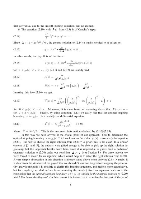
first derivative, due to the smooth pasting condition, has no atoms).6. The equation (2.10) with L X from (2.3) is of Cauchy’s type:(2.14) 22 x2 y 00 + xy 0 = c .Since 1 := 1 0 2= 2 6= 0 , the general solution to (2.14) is easily verified to be given by:(2.15) y = Ax 1 0 2c1 2 log(x) + B .In other words, the payoff is of the form:(2.16) V (x; s) = A(s)x 1 0 2c log(x) + B(s)12 for0 < g3(s) < x < s . By (2.11) and (2.12) we readily find:(2.17) A(s) =2c1 2 2 g3(s) 1(2.18) B(s) = s + 2c1 2 log g3(s)02c1 2 2 .Inserting this into (2.16) we get:(2.19) V (x; s) = 2c1 2 2 xg3(s)!10 logxg3(s)!10 1!for 0 < g3(s) < x < s . Moreover, it is clear from our reasoning above that V (x; s) = sfor 0 < x g3(s) . Finally, by using condition (2.13) we easily find that the optimal stoppingboundary s 7! g3(s) is to satisfy the differential equation:(2.20) g 0 (s) = K g(s)1+1s 1 0g(s) 1 (s > 0)where K = 1 2 =2c . This is the maximum information obtained by (2.10)-(2.13).7. In this way we have arrived at the crucial point of our approach: how to determine theoptimal stopping boundary s 7! g3(s) ? All we know so far is that g3(s) is to satisfy the equation(2.20). But how to choose the right solution from (2.20)? A priori this is not clear. In a similarcontext of [5] and [9], the authors were gifted enough to be able to pick up the right solution byguessing, but this approach breaks down here, since it is impossible to guess even a particular(nonzero) solution to (2.20) under our condition 1 > 1 ( see Section 3 ). For these reasons wewere forced to search for an argument which would help us to select the right solution from (2.20).A very simple observation in this direction is already stated above when deriving (2.8). Namely, itis clear from the structure of the payoff that we shouldn’t wait too long before stopping the process.(By analytic methods it is possible to clarify this intuitive argument, and make it more quantitative,but for simplicity we shall refrain from presenting the details.) Such an argument leads us to theconclusion that the optimal stopping boundary s 7! g3(s) should be the maximal solution to (2.20)which lies below the diagonal. (In this context it is instructive to examine the last part of the proof+ s5