inequality for geometric Brownian motion

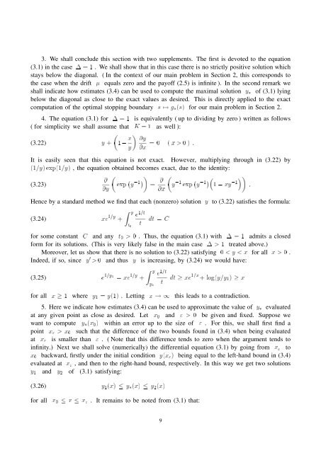
3. We shall conclude this section with two supplements. The first is devoted to the equation(3.1) in the case 1 = 1 . We shall show that in this case there is no strictly positive solution whichstays below the diagonal. ( In the context of our main problem in Section 2, this corresponds tothe case when the drift equals zero and the payoff (2.5) is infinite ). In the second remark weshall indicate how estimates (3.4) can be used to compute the maximal solution y3 of (3.1) lyingbelow the diagonal as close to the exact values as desired. This is directly applied to the exactcomputation of the optimal stopping boundary s 7! g3(s) for our main problem in Section 2.4. The equation (3.1) for 1 = 1 is equivalently ( up to dividing by zero ) written as follows( for simplicity we shall assume that K = 1 as well ):(3.22) y +10 x y @y@x = 0 ( x > 0 ) .It is easily seen that this equation is not exact. However, multiplying through in (3.22) by(1=y) exp(1=y) , the equation obtained becomes exact, due to the identity:@(3.23)@yexp0 011y = exp0 01@xy @ 01 y0111 0 xy .Hence by a standard method we find that each (nonzero) solution y to (3.22) satisfies the formula:(3.24) xe 1=y +Zye 1=tt 0tdt = Cfor some constant C and any t 0 > 0 . Thus, the equation (3.1) with 1 = 1 admits a closedform for its solutions. (This is very likely false in the main case 1 > 1 treated above.)Moreover, let us show that there is no solution to (3.22) satisfying 0 < y < x for all x > 0 .Indeed, if so, since y 0 > 0 and thus y is increasing, by (3.24) we would have:(3.25) e 1=y 1= xe 1=y +Zye 1=ty 1tdt xe 1=x + log(y=y 1 ) xfor all x 1 where y 1 = y(1) . Letting x ! 1 this leads to a contradiction.5. Here we indicate how estimates (3.4) can be used to approximate the value of y3 evaluatedat any given point as close as desired. Let x 0 and " > 0 be given and fixed. Suppose wewant to compute y3(x 0 ) within an error up to the size of " . For this, we shall first find apoint x " > x 0 such that the difference of the two bounds found in (3.4) when being evaluatedat x " is smaller than " . ( Note that this difference tends to zero when the argument tends toinfinity.) Next we shall solve (numerically) the differential equation (3.1) by going from x " tox 0 backward, firstly under the initial condition y(x " ) being equal to the left-hand bound in (3.4)evaluated at x " , and then to the right-hand bound, respectively. In this way we get two solutionsy 1 and y 2 of (3.1) satisfying:(3.26) y 1 (x) y3(x) y 2 (x)for allx 0 x x " . It remains to be noted from (3.1) that:9