Non-uniform sampling and spiral MRI reconstruction - Math ...

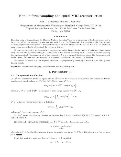
where |λ−γ| is the Euclidean distance between λ and γ. Fourier frames will be defined in Section 3, but a consequenceof their definition in the assertion of Beurling’s Theorem is that every finite energy signal f defined on E has therepresentationf(x) = ∑ λ∈Λa λ (f)e 2πi (1)in L 2 -norm on E, where ∑ λ∈Λ |a λ(f)| 2 < ∞. Beurling used the term “set of sampling” instead of “Fourier frame”.We shall reformulate Beurling’s Theorem in Theorem 7.2, in terms of a covering condition; and we shall referto Theorem 7.2 as the Beurling Covering Theorem. Beurling’s Theorem stated above becomes an obvious corollary.Our interest in this topic goes back to a problem about fast magnetic resonance imaging (MRI) posed to us by DennisHealy. Besides the present approach to non-uniform sampling using the power of Beurling’s results, there are otherapproaches 2 . 3In Section 2, we shall discuss the Classical Uniform Sampling Theorem for perspective with the result in Section 7and for ultimately comparing lattice and tiling ideas with analogous notions from non-uniform sampling. Fourierframes are introduced Section 3 in order to have a convenient structure in which to develop non-uniform samplingformulas. Section 4 is devoted to a discussion of density criteria in the setting of completeness results, and suchcriteria are essential for understanding effective signal reconstruction from non-uniformly spaced sampled values. Westate the fundamental characterization of Fourier frames in terms of density in Section 5.The notion of balayage is defined in Section 6; and Beurling’s theorem (1959), 4 describing the fundamentalrelationship between balayage and Fourier frames, is stated. This relationship is an essential component of theBeurling Covering Theorem in Section 7. We also take the opportunity to make some preliminary comments aboutrelated on-going work relating dimensionality, tilings, lattices, and coverings.In Section 8 we shall use the Beurling Covering Theorem to solve a mathematical version of the aforementionedproblem concerning fast MRI. 5 Basically, spectral (Fourier transform) data of an unknown signal f is given on adiscrete subset of finitely many interleaving spirals contained in ̂R 2 ; and the problem is to extract the original signalf ∈ L 2 (R 2 ) from this data whenever possible. Our solution is contained in Examples 2 and 3. In these examples, weshall provide a proof and algorithm for characterizing and constructing a uniformly discrete spectral subset Λ ⊆ ̂R 2on given interleaving spirals with the property that Λ is a Fourier frame in the sense of (1).Complete proofs of the aforementioned results, along with an analysis and history of the various relevant conceptsof density, will appear in a forthcoming research tutorial, 6 which also contains a complete bibliography.1.2. NotationWe shall use standard notation from harmonic analysis 7 . 8Further, M( ̂R d ) is the convolution algebra of bounded Radon measures on ̂R d ; and, if Λ ⊆ ̂R d is closed, thenM(Λ) denotes the closed subspace of M( ̂R) d consisting of those elements supported by Λ. Integration over Euclideanspace will be denoted by “ ∫ ”; and the Fourier transform ̂f of f defined on R d is formally given by∫ϕ(γ) = ̂f(γ) = f(x)e −2πi dx,where γ ∈ ̂R d . A(R d ) is the space of absolutely convergent inverse Fourier transforms on R d ,andA ′ (R d ), its dualspace when A(R d ) is normed by‖ϕ ∨ ‖ A(R d ) = ‖ϕ‖ L 1 (R d ),is the space of pseudo-measures on R d . B b (E) is the space of bounded continuous functions ϕ on ̂R d for whichsupp ϕ ∨ ⊆ E, where E is closed and ϕ ∨ is the distributional inverse Fourier transform of ϕ. Clearly, B b (E) ∧ ⊆ A ′ (R d ).Finally, we write e λ (x) =e 2πi for x ∈ R d and γ ∈ ̂R d .

Definition 3.3 (Fourier Frames).a. Let R>0, and assume that the sequence {e λ : λ ∈ Λ} is a frame for H = L 2 [−R, R]. This is clearly equivalentto the assertion that there exist A, B > 0 such that∀F ∈ PW R ,A‖F ‖ 2 L 2 (̂R) ≤ ∑ λ∈Λ|F (λ)| 2 ≤ B‖F ‖ 2 L 2 (̂R) . (6)As such we say that {e λ : λ ∈ Λ} is a Fourier frame for L 2 [−R, R], and by (5) we have∀f ∈ L 2 [−R, R], f = ∑ λ∈Λa λ (f)e λ in L 2 [−R, R]. (7)(7) is a non-harmonic Fourier series, see Chapter VII of Paley and Wiener. 10b. The frame radius R f (Λ) of Λ isR f (Λ) = sup{R ≥ 0:{e λ } is a Fourier frame for L 2 [−R, R]}.Example 1. Let us switch the notation R d and ̂R d in Theorem 2.3. We let Λ ⊆ ̂R d be a lattice, and we letE ⊆ R d be a unit cell of the reciprocal lattice. Then, if F ∈ L 2 ( ̂R d ) is a continuous function with the property thatf = F ∨ =0a.e. off of E, we have the sampling formulain L 2 (R). More generally, if Λ ⊆ ̂R d is a Fourier frame for PW E , then( )f(x) = 1 ∑F (λ)e 2πi 1 E (x) (8)|E|λ∈Λ∀f ∈ L 2 (E),f(x) = ∑ λ∈Λc λ e 2πiin L 2 (E), which can be compared with (8).4. DENSITY CRITERIA FOR COMPLETENESSIn order to gain insight into the structure of sets Λ ⊆ ̂R d for which {e λ : λ ∈ Λ} is a Fourier frame for PW E forsome E ⊆ R d , it is reasonable to consider first criteria for which {e λ : λ ∈ Λ} is complete in the case Λ ⊆ ̂R. Tobeprecise we let Λ = {λ k : k ∈ Z, λ −1 < 0 ≤ λ 0 , and lim k→±∞ λ k = ±∞} ⊆ ̂R be a strictly increasing sequence, whichis uniformly discrete or separated in the sense that∃r >0 such that ∀k ∈ Z, λ k+1 − λ k ≥ r.Further, for each R>0, we letX R = span {e λ : λ ∈ Λ}denote the closed linear span of {e λ : λ ∈ Λ} in L 2 [−R, R]. Paley and Wiener 10 (Chapter VI) refer to X R as the“closure” of the set {e λ : λ ∈ Λ} of complex exponential functions. If X R = L 2 [−R, R], then {e λ : λ ∈ Λ} is completein L 2 [−R, R].Definition 4.1 (The Closure of Sets of Complex Exponential Functions).a. The radius of completeness R c (Λ) of Λ isR c (Λ) = sup{R ≥ 0:X R = L 2 [−R, R]}.R c (Λ) is well-defined since it is clear that if R 1

R>R c (Λ). R c (Λ) is equal to the radii of completeness for the L p -spaces L p [−R, R], 1 ≤ p0 let n(γ) be the cardinalityof {λ k : k ≥ 1 and λ k ≤ γ}. Ifn(γ)lim > 2R, (9)γ→∞ γthen X R = L 2 [−R, R].Remark 2 (Completeness and Density).a. The “lim” on the left side of (9) is a density condition, and such conditions are essential hypotheses, notonly for completeness theorems such as Theorem 4.2 and Equation (15) below, but also for non-uniform samplingformulas.In engineering terms and in the context of non-uniform sampling, we can expect completeness if the number ofsamples per unit time exceeds on average twice the largest frequency in the given signal, i.e., if the average samplingrate exceeds the Nyquist rate. This sampling criteria is a density condition, and accurately quantifying the correctdensity to obtain completeness is difficult.Further, there are genuine engineering applications of some of these completeness theorems in uniquely determiningsignals from their non-uniformly spaced samples, e.g., Beutler’s work (1966) using results of Levinson.b. Paley and Wiener’s book (1934) 10 is the progenitor and driving force for an extensive and deep theory relatingrefinements of Theorem 4.2 with various notions of density, see Definition 4.3. Some of the many notable works sincethen are due to Levinson (1940), Duffin-Eachus (1942) and Duffin-Schaeffer 9 (1952), Kahane (1962), Beurling andLandau, e.g., Landau 11 (1967), and Beurling and Malliavin (1962 and 1967).There are also world class expositions due to Koosis (1970 and 1996) and Redheffer (1977) reflecting the authors’profound understanding of the problems and their own seminal contributions from the 1960s, cf., Boas’ book (1954)and a more recent and justly influential book due to Young (1980).This material is expanded as background in a forthcoming tutorial on multidimensional non-uniform sampling. 6Definition 4.3 (Density Criteria).Let Λ = {λ k : k ∈ Z, λ −1 < 0 ≤ λ 0 , and lim k→±∞ λ k = ±∞} ⊆ ̂R be a strictly increasing uniformly discretesequence, and define the functionn Λ = ∑ k1 [λk ,λ k+1 )whose distributional derivative is n ′ Λ = ∑ λ∈Λ δ λ. Clearly, if n :(0, ∞) →{0, 1,...} is defined by n(γ) =card{λ k :|λ k |≤γ}, where “card” is cardinality, then n(γ) =n Λ (γ) − n Λ (−γ).a. A reasonable definition of the density of Λ isn(γ)limγ→∞ 2γwhen this limit exists. As such, and since n Λ (γ k )=k, we shall define the natural density of Λ asD n (Λ) =lim|k|→∞kλ k(10)when the limit in (10) exists. Otherwise, we consider the upper, resp., lower, natural densitiesD + n (Λ) =b. Λ has uniform density D u (Λ) > 0iflim|k|→∞kλ k, resp., D − n (Λ) = lim|k|→∞kλ k.

Definition 6.2. Let E ⊆ R d be a symmetric body with polar set E ∗ . An entire function ϕ on C d is of exponentialtype E ∗ if∀ɛ >0, ∃A ɛ > 0such that∀z ∈ C d , |ϕ(z)| ≤A ɛ e 2π(1+ɛ)‖z‖E .The classical Plancherel-Pólya Theorem, originally proved on R, has the following formulation on R d , see pages108–114 of Stein and Weiss. 8Theorem 6.3. (Plancherel-Pólya Theorem) Let E be a symmetric body and let p>1. Ifϕ is an entire function ofexponential type E ∗ , then(∫) 1/p∀ξ ∈ ̂R d , |ϕ(γ + iξ)| p dγ ≤ e 2π‖ξ‖ E ∗ ‖ϕ‖Lp (̂R d ).̂R dThe Plancherel-Pólya Theorem can be used to prove the following Paley-Wiener Theorem. Generally, we shalluse the elementary sufficient conditions of the Paley-Wiener Theorem in order to obtain a function of exponentialtype; and then we use this property of a given function in order to invoke Plancherel-Pólya.Theorem 6.4. (Paley-Wiener Theorem) Let E ⊆ R d be a symmetric body, and let ϕ ∈ L 2 ( ̂R d ).Thensupp ϕ ∨ ⊆ Eif and only if ϕ is the restriction to ̂R d of an entire function of exponential type E ∗ .Definition 6.5. a. Let E ⊆ R d , and let μ, ν ∈ M( ̂R d ). The notation μ ∼ E ν denotes the property that μ ∨ = ν ∨on E.b. Let E ⊆ R d ,andletΛ⊆ ̂R d be a closed set. Balayage is possible for (E,Λ) if∀μ ∈ M( ̂R d ), ∃ν ∈ M(Λ) such that μ ∨ = ν ∨ on E,i.e., for each μ ∈ M( ̂R d ), there is a ν ∈ M(Λ) such that μ ∼ E ν.The following is a consequence of the Open Mapping Theorem.Let E ⊆ R d ,andletΛ⊆ ̂R d be a closed set. Assume balayage is possible for (E,Λ). There is K>0 such that∀μ ∈ M( ̂R d ),inf ‖ν‖ M(Λ) ≤ K‖μ‖ . (17)ν∈M(Λ),μ∼ M(̂R Eν d )The infimum of those K for which (17) holds is designated K(E,Λ).Beurling considered the following two properties on a closed set E ⊆ R d .(α) For each x 0 ∈ E and each ɛ>0, there is μ ɛ ∈ M(B(x 0 ,ɛ) ∩ E) such that lim |γ|→∞ ̂μ ɛ (γ) =0;(β) E is a set of spectral synthesis, i.e., T (f) = 0 for all f ∈ A(R d ) and all T ∈ A ′ (R d ) with the properties thatf =0onE and supp T ∈ A ′ (R d ).Clearly, if int E ≠ 0, then condition (α) is satisfied. There are other equivalent formulations of condition (β).For example, condition (β) is satisfied if and only if ∫ ϕ(γ) dμ(γ) = 0 for all ϕ ∈B b (E) and all μ ∈ M( ̂R d ) with theproperty that μ ∨ =0onE. We shall use the fact that closed, convex sets E ⊆ R d are sets of spectral synthesis.The following result was proved by Beurling. 4Lemma 6.6. Let E ⊆ R d be a compact set satisfying properties (α) and (β), andletE ɛ = {x : dist(x, E) ≤ ɛ}. IfK(E,Λ) < ∞, then there exists ɛ 0 such that∀ 0

and consequently the ordinary distance, from any point on the spiral A k to Λ k is less than δ. Finally, we setΛ R = ∪ M−1k=0 Λ k. Thus, by the triangle inequality,∀ξ ∈ ̂R 2 , dist(ξ,Λ R ) ≤ dist(ξ,B) + dist(B,Λ R ) ≤ c2M + δ = ρ.Hence, Rρ < 1/4 by our choice of M and δ; and so we can invoke Beurling’s Covering Theorem, Theorem 7.2, or theoriginal formulation state in the Introduction, to conclude that Λ R is a Fourier frame for PW B(0,R).Note that since we are reconstructing signals on a space domain having area about R 2 , we require essentially Rinterleaving spirals. On the other hand, if we are allowed to choose the spiral(s) after we are given PW B(0,R), thenwe can choose Λ R contained in a single spiral A c for c>0 small enough.REFERENCES1. A. Beurling, “Local harmonic analysis with some applications to differential operators,” in Proc. Annual ScienceConference, pp. 109–125, Belfer Graduate School of Science, 1966.2. J. J. Benedetto, “Irregular sampling and frames,” in Wavelets–A Tutorial in Theory and Applications, C.K.Chui, ed., pp. 445–507, Academic Press, Boston, 1992.3. K. Grochenig, “Non-uniform sampling in higher dimensions: from trigonometric polynomials to bandlimitedfunctions,” in Modern Sampling Theory: Mathematics and Applications, J. Benedetto and P. Ferreira, eds.,p. Chapter 7, Birkhauser, Boston, 2000.4. A. Beurling, “On balayage of measures in Fourier transforms (Seminar, Inst. for Advanced Studies, 1959–60,unpublished),” in Collected Works of Arne Beurling, L. Carleson, P. Malliavin, J. Neuberger, and J. Wermer,eds., Birkhauser, Boston, 1989.5. M. Bourgeois, F. T. A. W. Wajer, D. van Ormondt, and D. Graveron-Demilly, “Reconstruction of MRI imagesfrom non-uniform sampling, application to intrascan motion correction in functional MRI,” in Modern SamplingTheory: Mathematics and Applications, J. Benedetto and P. Ferreira, eds., p. Chapter 16, Birkhauser, Boston,2000.6. J. Benedetto and H.-C. Wu, “The Beurling-Landau theory of Fourier frames and applications,” J. FourierAnalysis and Applications 6, 2000.7. J. J. Benedetto, Harmonic Analysis and Applications, CRC Press, Inc., Boca Raton, FL, 1997.8. E. Stein and G. Weiss, An Introduction to Fourier Analysis on Euclidean Space, Princeton University Press,Princeton, NJ, 1971.9. R. J. Duffin and A. C. Schaeffer, “A class of nonharmonic Fourier series,” Trans. Amer. Math. Soc. 72, pp. 341–366, 1952.10. R. Paley and N. Wiener, Fourier transforms in the complex domain, Amer. Math. Soc. Colloquium Publ. 19,New York, 1934.11. H. J. Landau, “Necessary density conditions for sampling and interpolation of certain entire function,” ActaMath. 117, pp. 37–52, 1967.12. S. Jaffard, “A density criterion for frames of complex exponentials,” Michigan Math. J. 38, pp. 339–348, 1991.