Introduction to Shimura varieties with bad reduction of parahoric type

Clay Mathematics ProceedingsVolume 4, 2005Introduction to Shimura Varieties withBad Reduction of Parahoric TypeThomas J. HainesContents1. Introduction 5832. Notation 5843. Iwahori and parahoric subgroups 5874. Local models 5895. Some PEL Shimura varieties with parahoric level structure at p 5936. Relating Shimura varieties and their local models 6027. Flatness 6088. The Kottwitz-Rapoport stratification 6099. Langlands’ strategy for computing local L-factors 61410. Nearby cycles 61811. The semi-simple local zeta function for “fake” unitaryShimura varieties 62112. The Newton stratification on Shimura varieties over finite fields 62813. The number of irreducible components in Sh Fp63414. Appendix: Summary of Dieudonné theory and de Rham and crystallinecohomology for abelian varieties 636References 6401. IntroductionThis survey article is intended to introduce the reader to several importantconcepts relating to Shimura varieties with parahoric level structure at p. Themain tool is the Rapoport-Zink local model [RZ], which plays an important rolein several aspects of the theory. We discuss local models attached to general linearand symplectic groups, and we illustrate their relation to Shimura varieties intwo examples: the simple or “fake” unitary Shimura varieties with parahoric levelstructure, and the Siegel modular varieties with Γ 0 (p)-level structure. In addition,we present some applications of local models to questions of flatness, stratificationsResearch partially supported by NSF grant DMS 0303605.583c○ 2005 Clay Mathematics Institute

584 THOMAS J. HAINESof the special fiber, and the determination of the semi-simple local zeta functionsfor simple Shimura varieties.There are several good references for material of this sort that already exist inthe literature. This survey has a great deal of overlap with two articles of Rapoport:[R1] and [R2]. A main goal of this paper is simply to make more explicit someof the ideas expressed very abstractly in those papers. Hopefully it will shed somenew light on the earlier seminal works of Rapoport-Zink [RZ82], and Zink [Z].This article is also closely related to some recent work of H. Reimann [Re1], [Re2],[Re3].Good general introductions to aspects of the Langlands program which mightbe consulted while reading parts of this report are those of Blasius-Rogawski [BR],and T. Wedhorn [W2].Several very important developments have taken place in the theory of Shimuravarieties with bad reduction, which are completely ignored in this report. In particular,we mention the book of Harris-Taylor [HT] which uses bad reduction ofShimura varieties to prove the local Langlands conjecture for GL n (Q p ), and therecent work of L. Fargues and E. Mantovan [FM].Most of the results stated here are well-known by now (although scatteredaround the literature, with differing systems of conventions). However, the authortook this opportunity to present a few new results (and some new proofs of oldresults). For example, there is the proof of the non-emptiness of the Kottwitz-Rapoport strata in any connected component of the Siegel modular and “fake”unitary Shimura varieties with Iwahori-level structure (Lemmas 13.1, 13.2), somefoundational relations between Newton strata, Kottwitz-Rapoport strata, and affineDeligne-Lusztig varieties (Prop. 12.6), and the verification of the conjectural nonemptinessof the basic locus in the “fake” unitary case (Cor. 12.12). The main newproofs relate to topological flatness of local models attached to Iwahori subgroupsof unramified groups (see §7) and to the description of the nonsingular locus ofShimura varieties with Iwahori-level structure (see §8.4). Finally, some of the resultsexplained here (especially in §11) are background material necessary for the author’sas yet unpublished joint work with B.C. Ngô [HN3].I am grateful to U. Görtz, R. Kottwitz, B.C. Ngô, G. Pappas, and M. Rapoportfor all they have taught me about this subject over the years. I thank them for theirvarious comments and suggestions on an early version of this article. Also, I heartilythank U. Görtz for providing the figures. Finally, I thank the Clay MathematicsInstitute for sponsoring the June 2003 Summer School on Harmonic Analysis, theTrace Formula, and Shimura Varieties, which provided the opportunity for me towrite this survey article.2. Notation2.1. Some field-theoretic notation. Fix a rational prime p. We let F denotea non-Archimedean local field of residual characteristic p, with ring of integersO. Let p ⊂ O denote the maximal ideal, and fix a uniformizer π ∈ p. The residuefield O/p has cardinality q, a power of p.We will fix an algebraic closure k of the finite field F p . The Galois groupGal(k/F p ) has a canonical generator (the Frobenius automorphism), given by σ(x) =x p . For each positive integer r, we denote by k r the fixed field of σ r . Let W(k r )(resp. W(k)) denote the ring of Witt vectors of k r (resp. k), with fraction field L r

SHIMURA VARIETIES WITH PARAHORIC LEVEL STRUCTURE 585(resp. L). We also use the symbol σ to denote the Frobenius automorphism of Linduced by that on k.We fix throughout a rational prime l ≠ p, and a choice of algebraic closureQ l ⊂ Q l .2.2. Some group-theoretic notation. The symbol G will always denote aconnected reductive group over Q (sometimes defined over Z). Unless otherwiseindicated, G will denote the base-change G F , where F is a suitable local field(usually, G = G Qp ).Now let G denote a connected reductive F-group. Fix once and for all a Borelsubgroup B and a maximal torus T contained in B. We will usually assume G issplit over F, in which case we can even assume G, B and T are defined and splitover the ring O. For GL n or GSp 2n , T will denote the usual “diagonal” torus, andB will denote the “upper triangular” Borel subgroup.We will often refer to “standard” parahoric and “standard” Iwahori subgroups.For the group G = GL n (resp. G = GSp 2n ), the “standard” hyperspecial maximalcompact subgroup of G(F) will be the subgroup G(O). The “standard” Iwahorisubgroup will be inverse image of B(O/p) under the reduction modulo p homomorphismG(O) → G(O/p).A “standard” parahoric will be defined similarly as the inverse image of a standard(= upper triangular) parabolic subgroup.For GL n (F), the standard Iwahori is the subgroup stabilizing the standardlattice chain (defined in §3). The standard parahorics are stabilizers of standardpartial lattice chains. Similar remarks apply to the group GSp 2n (F). The symbolsI or I r or Kp a will always denote a standard Iwahori subgroup of G(F) defined interms of our fixed choices of B ⊃ T, and G(O) as above (for some local field F).Often (but not always) K or K r or Kp 0 will denote our fixed hyperspecial maximalcompact subgroup G(O).We have the associated spherical Hecke algebra H K := C c (K\G(F)/K), a convolutionalgebra of C-valued (or Q l -valued) functions on G(F) where convolutionis defined using the measure giving K volume 1. Similarly, H I := C c (I\G(F)/I)is a convolution algebra using the measure giving I volume 1. For a compact opensubset U ⊂ G(F), I U denotes the characteristic function of the set U.The extended affine Weyl group of G(F) is defined as the group˜W = N G(F) T/T(O). The map X ∗ (T) → T(F)/T(O) given by λ ↦→ λ(π) is anisomorphism of abelian groups. The finite Weyl group W 0 := N G(F) T/T(F) canbe identified with N G(O) T/T(O), by choosing representatives of N G(F) T/T(F) inG(O). Thus we have a canonical isomorphism˜W = X ∗ (T) ⋊ W 0 .We will denote elements in this group typically by the notation t ν w (for ν ∈ X ∗ (T)and w ∈ W 0 ).Our choice of B ⊃ T determines a unique opposite Borel subgroup ¯B such thatB∩ ¯B = T. We have a notion of B-positive (resp. ¯B-positive) root α and coroot α ∨ .Also, the group W 0 is a Coxeter group generated by the simple reflections s α in thevector space X ∗ (T) ⊗ R through the walls fixed by the B-positive (or ¯B-positive)simple roots α. Let w 0 denote the unique element of W 0 having greatest lengthwith respect to this Coxeter system.

586 THOMAS J. HAINESWe will often need to consider ˜W as a subset of G(F). We choose the followingconventions. For each w ∈ W 0 , we fix once and for all a lift in the group N G(O) T.We identify each ν ∈ X ∗ (T) with the element ν(π) ∈ T(F) ⊂ G(F).Let a denote the alcove in the building of G(F) which is fixed by the IwahoriI, or equivalently, the unique alcove in the apartment corresponding to T whichis contained in the ¯B-positive (i.e., the B-negative) Weyl chamber, whose closurecontains the origin (the vertex fixed by the maximal compact subgroup G(O)) 1 .The group ˜W permutes the set of affine roots α + k (α a root, k ∈ Z) (viewedas affine linear functions on X ∗ (T) ⊗ R), and hence permutes (transitively) the setof alcoves. Let Ω denote the subgroup which stabilizes the base alcove a. Then wehave a semi-direct product˜W = W aff ⋊ Ω,where W aff (the affine Weyl group) is the Coxeter group generated by the reflectionsS aff through the walls of a. In the case where G is an almost simple group of rank l,with simple B-positive roots α 1 , . . .,α l , then S aff consists of the l simple reflectionss i = s αi generating W 0 , along with one more simple affine reflection s 0 = t −eα ∨s eα ,where ˜α is the highest B-positive root.The Coxeter system (W aff , S aff ) determines a length function l and a Bruhatorder ≤ on W aff , which extend naturally to ˜W: for x i ∈ W aff and σ i ∈ Ω (i = 1, 2),we define x 1 σ 1 ≤ x 2 σ 2 in ˜W if and only if σ 1 = σ 2 and x 1 ≤ x 2 in W aff . Similarly,we set l(x 1 σ 1 ) = l(x 1 ).By the Bruhat-Tits decomposition, the inclusion ˜W ֒→ G(F) induces a bijection˜W = I\G(F)/I.In the function-field case (e.g., F = F p ((t))), the affine flag variety Fl = G(F)/Iis naturally an ind-scheme, and the closures of the I-orbits Fl w := IwI/I aredetermined by the Bruhat order on ˜W:Fl x ⊂ Fl y ⇐⇒ x ≤ y.Similar statements hold for the affine Grassmannian, Grass = G(F)/G(O).Now the G(O)-orbits Q λ := G(O)λG(O)/G(O) are given (using the Cartan decomposition)by the B-dominant coweights X + (T):X + (T) ↔ G(O)\G(F)/G(O).By definition, λ is B-dominant if 〈α, λ〉 ≥ 0 for all B-positive roots α. Here 〈·, ·〉 :X ∗ (T) × X ∗ (T) → Z is the canonical duality pairing.The closure relations in Grass are given by the partial order on B-dominantcoweights λ and µ:Q λ ⊂ Q µ ⇐⇒ λ ≼ µ,where λ ≺ µ means that µ − λ is a sum of B-positive coroots.Unless otherwise stated, a dominant coweight λ ∈ X ∗ (T) will always mean onethat is B-dominant.For the group G = GL n or GSp 2n , there is a Z p -ind-scheme M which is adeformation of the affine Grassmannian Grass Qp to the affine flag variety Fl Fpfor the underlying p-adic group G (see [HN1], and Remark 4.1). A very similar1 This choice of base alcove results from our convention of embedding X∗(T) ֒→ G(F) by therule λ ↦→ λ(π); to see this, consider how vectors spanning the standard periodic lattice chain in§3 are identified with vectors in X ∗(T) ⊗ R.

SHIMURA VARIETIES WITH PARAHORIC LEVEL STRUCTURE 587deformation Fl X over a smooth curve X (due to Beilinson) exists for any group Gin the function field setting, and has been extensively studied by Gaitsgory [Ga].For any dominant coweight λ ∈ X + (T), the symbol M λ will always denote theZ p -scheme which is the scheme-theoretic closure in M of Q λ ⊂ Grass Qp .2.3. Duality notation. If A is any abelian scheme over a scheme S, we denotethe dual abelian scheme by Â. The existence of  over an arbitrary base is a delicatematter; see [CF], §I.1.If M is a module over a ring R, we denote the dual module by M ∨ = Hom R (M,R).Similar notation applies to quasi-coherent O S -modules over a scheme S.If G is a connected reductive group over a local field F, then the Langlandsdual (over C or Q l ) will be denoted Ĝ. The Langlands L-group is the semi-directproduct L G = Ĝ ⋊ W F, where W F is the Weil-group of F.2.4. Miscellaneous notation. We will use the following abbreviation for elementsof R n (here R can be any set): let a 1 , . . . , a r be a sequence of positive integerswhose sum is n. A vector of the form (x 1 , . . . , x 1 , x 2 , . . . , x 2 , . . . , x r , . . . , x r ), wherefor i = 1, . . .,r, the element x i is repeated a i times, will be denoted by(x a11 , xa2 2 , . . . , xar r ).We will denote by A the adeles of Q, by A f the finite adeles, and by A p f thefinite adeles away from p (with the exception of two instances, where A denotesaffine space!).3. Iwahori and parahoric subgroups3.1. Stabilizers of periodic lattice chains. We discuss the definitions forthe groups GL n and GSp 2n .3.1.1. The linear case. For each i ∈ {1, . . ., n}, let e i denote the i-th standardvector (0 i−1 , 1, 0 n−i ) in F n , and let Λ i ⊂ F n denote the free O-module with basisπ −1 e 1 , . . . , π −1 e i , e i+1 , . . . , e n . We consider the diagramΛ • : Λ 0 −→ Λ 1 −→ · · · −→ Λ n−1 −→ π −1 Λ 0 ,where the morphisms are inclusions. The lattice chains π n Λ • (n ∈ Z) fit togetherto form an infinite complete lattice chain Λ i , (i ∈ Z). If we identify each Λ i withO n , then the diagram above becomesO n m 1 O n m2 · · · mn−1 O n m n O n ,where m i is the morphism given by the diagonal matrixm i = diag(1, . . . , π, . . . ,1),the element π appearing in the ith place. We define the (standard) Iwahori subgroupI of GL n (F) byI = ⋂ Stab GLn(F) (Λ i ).iSimilarly, for any non-empty subset J ⊂ {0, 1, . . ., n − 1}, we define the parahoricsubgroup of GL n (F) corresponding to the subset J byP J = ⋂ i∈JStab GLn(F) (Λ i ).

588 THOMAS J. HAINESNote that P J is a compact open subgroup of GL n (F), and that P {0} = GL n (O) isa hyperspecial maximal compact subgroup, in the terminology of Bruhat-Tits, cf.[T].3.1.2. The symplectic case. The definitions for the group of symplectic similitudesGSp 2n are similar. We define this group using the alternating matrixĨ =[0 Ĩn−Ĩn 0where Ĩn denotes the n × n matrix with 1 along the anti-diagonal and 0 elsewhere.Let (x, y) := x t Ĩy denote the corresponding alternating pairing on F 2n . For anO-lattice Λ ⊂ F 2n , we define Λ ⊥ := {x ∈ F 2n | (x, y) ∈ O for all y ∈ Λ}. Thelattice Λ 0 is self-dual (i.e., Λ ⊥ 0 = Λ 0). Consider the infinite lattice chain in F 2n· · · −→ Λ −2n = πΛ 0 −→ · · · −→ Λ −1 −→ Λ 0 −→ · · · −→ Λ 2n = π −1 Λ 0 −→ · · ·We have Λ ⊥ i = Λ −i for all i ∈ Z. Now we define the (standard) Iwahori subgroup Iof GSp 2n (F) byI = ⋂ i],Stab GSp2n (F) (Λ i ).For any non-empty subset J ⊂ {−n, . . ., −1, 0, 1, . . ., n} such that i ∈ J ⇔ −i ∈ J,we define the parahoric subgroup corresponding to J byP J = ⋂ i∈JStab GSp2n (F) (Λ i ).3.2. Bruhat-Tits group schemes. In Bruhat-Tits theory, parahoric groupsare defined as the groups G 0 ∆ J(O), where G 0 ∆ Jis the neutral component of a groupscheme G ∆J , defined and smooth over O, which has generic fiber the F-group G,and whose O-points are the subgroup of G(F) fixing the facet ∆ J of the Bruhat-Tits building corresponding to the set J; see [BT2], p. 356. By [T], 3.4.1 (see also[BT2], 1.7) we can characterize the group scheme G ∆J as follows: it is the uniqueO-group scheme P satisfying the following three properties:(1) P is smooth and affine over O;(2) The generic fiber P F is G F ;(3) For any unramified extension F ′ of F, letting O F ′ ⊂ F ′ denote ring ofintegers, the group P(O F ′) ⊂ G(F ′ ) is the subgroup of elements which fixthe facet ∆ J in the Bruhat-Tits building of G F ′.Let us show how automorphism groups of periodic lattice chains Λ • give aconcrete realization of the Bruhat-Tits parahoric group schemes, in the GL n andGSp 2n cases. We will discuss the Iwahori subgroups of GL n in some detail, leavingfor the reader the obvious generalizations to parahoric subgroups of GL n (andGSp 2n ).For any O-algebra R, we may consider the diagram Λ •,R = Λ • ⊗ O R, andwe may define the O-group scheme Aut whose R-points are the isomorphisms ofthe diagram Λ •,R . More precisely, an element of Aut(R) is an n-tuple of R-linearautomorphisms(g 0 , . . . , g n−1 ) ∈ Aut(Λ 0,R ) × · · · × Aut(Λ n−1,R )

SHIMURA VARIETIES WITH PARAHORIC LEVEL STRUCTURE 589such that the following diagram commutesΛ 0,R· · · Λ n−1,RΛ n,Rg 0g 0g n−1Λ 0,R · · · Λ n−1,R Λ n,R .The group functor Aut is obviously represented by an affine group scheme, alsodenoted Aut. Further, it is not hard to see that Aut is formally smooth, hencesmooth, over O. To show this, one has to check the lifting criterion for formalsmoothness: if R is an O-algebra containing a nilpotent ideal J ⊂ R, then anyautomorphism of Λ • ⊗ O R/J can be lifted to an automorphism of Λ • ⊗ O R. Thisis proved on page 135 of [RZ]. Thus Aut satisfies condition (1) above.Alcoves in the Bruhat-Tits building for GL n over F can be described as completeperiodic O-lattice chains in F n· · · −→ L 0 −→ L 1 −→ · · · −→ L n−1 −→ L n = π −1 L 0 −→ · · ·where the arrows are inclusions. We can regard Λ • as the base alcove in this building.It is clear that since π is invertible over the generic fiber F, the automorphismg 0 determines the other g i ’s over F and so Aut F = GL n . By construction we haveAut(O) = Stab GLn(F) (Λ • ). This is unchanged if we replace F by an unramifiedextension F ′ . It follows that Aut satisfies conditions (2) and (3) above. Thus, byuniqueness, Aut = G ∆J for J = {0, . . .,n − 1}.Further, one can check that the special fiber Aut k is an extension of the Borelsubgroup B k by a connected unipotent group over k; hence the special fiber isconnected. It follows that Aut is a connected group scheme (cf. [BT2], 1.2.12).So in this case Aut = G ∆J = G 0 ∆ J. We conclude that Aut(O) is the Bruhat-TitsIwahori subgroup fixing the base alcove Λ • .Exercise 3.1. 1) Check the lifting criterion which shows Aut is formallysmooth directly for the case n = 2, by explicit calculations with 2 × 2 matrices.2) By identifying Aut(O) with its image in GL n (F) under the inclusion g • ↦→g 0 , show that the Iwahori subgroup is the preimage of B(k) under the canonicalsurjection GL n (O) → GL n (k).3) Prove that Aut k → Aut(Λ 0,k ), g • ↦→ g 0 , has image B k , and kernel a connectedunipotent group.4. Local modelsGiven a certain triple (G, µ, K p ) consisting of a Z p -group G, a minusculecoweight µ for G, and a parahoric subgroup K p ⊂ G(Q p ), one may construct aprojective Z p -scheme M loc which (étale locally) models the singularities found inthe special fiber of a certain Shimura variety with parahoric-level structure at p.The advantage of M loc is that it is defined in terms of linear algebra and is thereforeeasier to study than the Shimura variety itself. These schemes are called “localmodels”, or sometimes “Rapoport-Zink local models”; the most general treatmentis given in [RZ], but in special cases they were also investigated in [DP] and [deJ].In this section we recall the definitions of local models associated to GL n andGSp 2n . For simplicity, we limit the discussion to models for Iwahori-level structure.In each case, the local model is naturally associated to a dominant minusculecoweight µ, which we shall always mention. In fact, it turns out that if the Shimura

590 THOMAS J. HAINESdata give rise to (G, µ), then the Rapoport-Zink local model M loc (for Iwahori-levelstructure) can be identified with the space M −w0µ mentioned in §2. See Remark4.1 below.4.1. Linear case. We use the notation Λ • from section 3 to denote the “standard”lattice chain over O = Z p here.Fix an integer d with 1 ≤ d ≤ n − 1. We define the scheme M loc by definingits R-points for any Z p -algebra R as the set of isomorphism classes of commutativediagramspΛ 0,R · · · Λ n−1,R Λ n,R Λ 0,RF 0 · · · F n−1 F np F 0where the vertical arrows are inclusions, and each F i is an R-submodule of Λ i,Rwhich is Zariski-locally on R a direct factor of corank d. It turns out that this isidentical to the space M −w0µ of §2, where µ = (0 n−d , (−1) d ). It is clear that M locis represented by a closed subscheme of a product of Grassmannians over Z p , henceit is a projective Z p -scheme. One can also formulate the moduli problem usingquotients of rank d instead of submodules of corank d.Another way to formulate the same moduli problem which is sometimes useful(see [HN1]) is given by adding an indeterminate t to the story (following a suggestionof G. Laumon). We replace the “standard” lattice chain term Λ i,R withV i,R := α −i R[t] n , where α is the n × n matrix⎛⎜⎝0 1. .. . ..0 1t + p 0⎞⎟⎠ ∈ GL n(R[t, t −1 , (t + p) −1 ]).One can identify M loc (R) with the set of chainsL • = (L 0 ⊂ L 1 ⊂ · · · ⊂ L n = (t + p) −1 L 0 )of R[t]-submodules of R[t, t −1 , (t + p) −1 ] n satisfying the following properties(1) for all i = 0, . . .,n − 1, we have tV i,R ⊂ L i ⊂ V i,R ;(2) as an R-module, L i /tV i,R is locally a direct factor of V i,R /tV i,R of corankd.Remark 4.1. With the second definition, it is easy to see that the geometricgeneric fiber M loc is contained in the affine Grassmannian GLQ n (Q p ((t)))/GL n (Q p [[t]]),pand the geometric special fiber M loc is contained in the affine flag varietyF pGL n (F p ((t)))/I Fp, where I Fp:= Aut(F p [[t]]) is the Iwahori subgroup of GL n (F p [[t]])corresponding to the upper triangular Borel subgroup B ⊂ GL n . Moreover, it ispossible to view M loc as a piece of a Z p -ind-scheme M which forms a deformationof the affine Grassmannian to the affine flag variety over the base Spec(Z p ), in analogywith Beilinson’s deformation Fl X over a smooth F p -curve X in the functionfield case (cf. [Ga], [HN1]). In fact, letting e 0 denote the base point in the affineGrassmannian GL n (Q p ((t)))/GL n (Q p [[t]]), and for λ ∈ X + (T), letting Q λ denotethe GL n (Q p [[t]])-orbit of the point λ(t)e 0 , it turns out that M loc coincides with

SHIMURA VARIETIES WITH PARAHORIC LEVEL STRUCTURE 591the scheme-theoretic closure M −w0µ of Q −w0µ taken in the model M. A similarstatement holds in the symplectic case.The identification M loc = M −w0µ is explained in §8. It is a consequence of thedeterminant condition and the “homology” definition of our local models; also theflatness of M loc (see §7) plays a role.4.2. The symplectic case. Recall that for our group GSp 2n = GSp(V, (·, ·)),we have an identification of X ∗ (T) with the lattice {(a 1 , . . . , a n , b n , . . . , b 1 ) ∈Z 2n | ∃ c ∈ Z, a i +b i = c, ∀i}. The Shimura coweight that arises here has the formµ = (0 n , (−1) n ).For the group GSp 2n , the symbol Λ • now denotes the self-dual Z p -lattice chainin Q 2np , discussed in section 3 in the context of GSp 2n . Let (·, ·) denote the alternatingpairing on Z 2np discussed in that section, and let the dual Λ ⊥ of a latticeΛ be defined using (·, ·). As above, there are (at least) two equivalent ways to defineM loc (R) for a Z p -algebra R. We define M loc (R) to be the set of isomorphismclasses of diagramsΛ 0,R · · · Λ n−1,R Λ n,RF 0 · · · F n−1 F nwhere the vertical arrows are inclusions of R-submodules with the following properties:(1) for i = 0, . . .,n, Zariski-locally on R the submodule F i is a direct factorof Λ i,R of corank n;(2) F 0 is isotropic with respect to (·, ·) and F n is isotropic with respect top(·, ·).As in the linear case, this can be described in a way more transparently connectedto affine flag varieties. In this case, V i,R has the same meaning as in thelinear case, except that the ambient space is now R[t, t −1 , (t + p) −1 ] 2n . We maydescribe M loc (R) as the set of chainsL • = (L 0 ⊂ L 1 ⊂ · · · ⊂ L n )of R[t]-submodules of R[t, t −1 , (t + p) −1 ] 2n satisfying the following properties(1) for i = 0, 1, . . ., n, tV i,R ⊂ L i ⊂ V i,R ;(2) as R-modules, L i /tV i,R is locally a direct factor of V i,R /tV i,R of corank n;(3) L 0 is self-dual with respect to t −1 (·, ·), and L n is self-dual with respect tot −1 (t + p)(·, ·).4.3. Generic and special fibers. In the linear case with µ = (0 n−d , (−1) d ),the generic fiber of M −w0µ is the Grassmannian Gr(d, n) of d-planes in Q n p. In thesymplectic case with µ = (0 n , (−1) n ), the generic fiber of M −w0µ is the Grassmannianof isotropic n-planes in Q 2np with respect to the alternating pairing (·, ·).In each case, the special fiber is a union of finitely many Iwahori-orbits IwI/Iin the affine flag variety, indexed by elements w in the extended affine Weyl group˜W for GL n (resp. GSp 2n ) ranging over the so-called −w 0 µ-admissible subsetAdm(−w 0 µ), [KR]. Let λ ∈ X + (T). Then by definitionAdm(λ) = {w ∈ ˜W | ∃ ν ∈ Wλ, such that w ≤ t ν }.

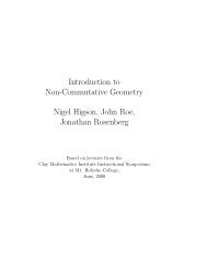
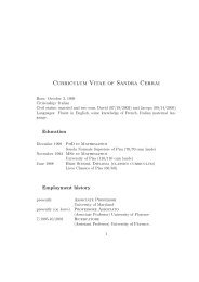
592 THOMAS J. HAINESHere, Wλ is the set of conjugates of λ under the action of the finite Weyl groupW 0 , and t ν ∈ ˜W is the translation element corresponding to ν, and ≤ denotes theBruhat order on ˜W. Actually (see §8.1), the set that arises naturally from themoduli problem is the −w 0 µ-permissible subset Perm(−w 0 µ) ⊂ ˜W from [KR]. Letus recall the definition of this set, following loc. cit. Let λ ∈ X + (T) and supposet λ ∈ W aff τ, for τ ∈ Ω. Then Perm(λ) consists of the elements x ∈ W aff τ such thatx(a) − a ∈ Conv(λ) for every vertex a ∈ a. Here Conv(λ) denotes the convex hullof Wλ in X ∗ (T) ⊗ R.The strata in the special fiber of M loc = M −w0µ are naturally indexed bythe set Perm(−w 0 µ), which agrees with Adm(−w 0 µ) by the following non-trivialcombinatorial theorem due to Kottwitz and Rapoport.Theorem 4.2 ([KR]; see also [HN2]). For every minuscule coweight λ ofeither GL n or GSp 2n , we have the equalityPerm(λ) = Adm(λ).Using the well-known correspondence between elements in the affine Weyl groupand the set of alcoves in the standard apartment of the Bruhat-Tits building, onecan “draw” pictures of Adm(µ) for low-rank groups. Figures 1 and 2 depict thisset for G = GL 3 , µ = (−1, 0, 0), and G = GSp 4 , µ = (−1, −1, 0, 0) 2 . Actually,we draw the image of Adm(µ) in the apartment for PGL 3 (resp. PGSp 4 ); the basealcove is labeled by τ.4.4. Computing the singularities in the special fiber of M loc . In certaincases, the singularities in M loc¯F pcan be analyzed directly by writing down equations.As the simplest example of how this is done, we analyze the local model for GL 2 ,µ = (0, −1). For a Z p -algebra R, we are looking at the set of pairs (F 0 , F 1 ) oflocally free rank 1 R-submodules of R 2 such that the following diagram commutes2643264p 01 077550 1 0 pR ⊕ R R ⊕ R R ⊕ R3F 0 F 1Obviously this functor is represented by a certain closed subscheme of P 1 Z p× P 1 Z p.Locally around a fixed point (F 0 , F 1 ) ∈ P 1 (R) × P 1 (R) we choose coordinates suchthat F 0 is represented by the homogeneous column vector [1 : x] t and F 1 by thevector [y : 1] t , for x, y ∈ R. We see that (F 0 , F 1 ) ∈ M loc (R) if and only ifxy = p,so M loc is locally the same as Spec(Z p [X, Y ]/(XY − p), the usual deformation ofA 1 Q pto a union of two A 1 F p’s which intersect transversally at a point. Indeed, M locis globally this kind of deformation:• In the generic fiber, the matrices are invertible and so F 0 uniquely determinesF 1 ; thus M locQ p∼ = P1Qp;2 Note that in Figure 2 there is an alcove of length one contained in the Bruhat-closure ofall four distinct translations. This already tells us something about the singularities: the specialfiber of the Siegel variety for GSp 4 is not a union of divisors with normal crossings; see §8. F 0

SHIMURA VARIETIES WITH PARAHORIC LEVEL STRUCTURE 593s 1s 0τs 1τs 0τ0τs 0s 2τ = t µs 2τs 2s 1τFigure 1. The admissible alcoves Adm(µ) for GL 3 , µ =(−1, 0, 0). The base alcove is labeled by τ.• In the special fiber, p = 0 and one can check that M locF pis the union of theclosures of two Iwahori-orbits in the affine flag variety GL 2 (F p ((t)))/I Fp ,each of dimension 1, which meet in a point. Thus M locF pis the union oftwo P 1 F p’s meeting in a point.We refer to the work of U. Görtz for many more complicated calculations ofthis kind: [Go1], [Go2], [Go3], [Go4].5. Some PEL Shimura varieties with parahoric level structure at p5.1. PEL-type data. Given a Shimura datum (G, {h},K) one can constructa Shimura variety Sh(G, h) K which has a canonical model over the reflex field E, anumber field determined by the datum. We write G for the p-adic group G Qp . Letus assume that the compact open subgroup K ⊂ G(A f ) is of the form K = K p K p ,where K p ⊂ G(A p f ) is a sufficiently small compact open subgroup, and K p ⊂ G(Q p )is a parahoric subgroup.Let us fix once and for all embeddings Q ֒→ C, and Q ֒→ Q p . We denote by pthe corresponding place of E over p and by E = E p the completion of E at p.If the Shimura datum comes from PEL-type data, then it is possible to definea moduli problem (in terms of chains of abelian varieties with additional structure)

594 THOMAS J. HAINESs 1s 0s 2τs 1s 0τs 0s 1s 0τ= t µs 1s 2τs 1τs 0s 1τ0τs 0τs 2τs 0s 2τs 2s 1s 2τs 2s 1τs 0s 2s 1τFigure 2. The admissible alcoves Adm(µ) for GSp 4 , µ = (−1, −1, 0, 0).over the ring O E . This moduli problem is representable by a quasi-projective O E -scheme whose generic fiber is the base-change to E of the initial Shimura varietySh(G, h) K (or at least a finite union of Shimura varieties, one of which is thecanonical model Sh(G, h) K ). This is done in great generality in Chapter 6 of [RZ].Our aim in this section is only to make somewhat more explicit the definitions inloc. cit., in two very special cases attached to the linear and symplectic groups.First, let us recall briefly PEL-type data. Let B denote a finite-dimensionalsemi-simple Q-algebra with positive involution ι. Let V ≠ 0 be a finitely-generatedleft B-module, and let (·, ·) be a non-degenerate alternating form V × V → Q onthe underlying Q-vector space, such that (bv, w) = (v, b ι w), for b ∈ B, v, w ∈ V .The form (·, ·) determines a “transpose” involution on End(V ), denoted by ∗ (soviewing the left-action of b as an element of End(V ), we have b ι = b ∗ ). We denoteby G the Q-group whose points in a Q-algebra R are{g ∈ GL B⊗R (V ⊗ R) | g ∗ g = c(g) ∈ R × }.We assume G is a connected reductive group; this means we are excluding theorthogonal case. Consider the R-algebra C := End B (V ) ⊗ R. We let h 0 : C → Cdenote an R-algebra homomorphism satisfying h 0 (z) = h 0 (z) ∗ , for z ∈ C. We fixa choice of i = √ −1 in C once and for all, and we assume the symmetric bilinearform (· , h 0 (i) ·) : V R × V R → R is positive definite. Let h denote the inverse of therestriction of h 0 to C × . Then h induces an algebraic homomorphismh : C × → G(R)

SHIMURA VARIETIES WITH PARAHORIC LEVEL STRUCTURE 595of real groups which defines on V R a Hodge structure of type (1, 0) + (0, 1) (in theterminology of [Del2], section 1) and which satisfies the usual Riemann conditionswith respect to (·, ·) (see [Ko92], Lemma 4.1). For any choice of (sufficientlysmall) compact open subgroup K, the data (G, h,K) determine a (smooth) Shimuravariety over a reflex field E; cf. [Del].We recall that h gives rise to a minuscule coweightµ := µ h : G m,C → G Cas follows: the complexification of the real group C × is the torus C × × C × , thefactors being indexed by the two R-algebra automorphisms of C; we assume the firstfactor corresponds to the identity and the second to complex conjugation. Thenwe defineµ(z) := h C (z, 1).By definition of Shimura data, the homomorphism h : C × → G R is only specified upto G(R)-conjugation, and therefore µ is only well-defined up to G(C)-conjugation.However, this conjugacy class is at least defined over the reflex field E (in fact wedefine E as the field of definition of the conjugacy class of µ). Via our choice offield embeddings C ←֓ Q ֒→ Q p , we get a well-defined conjugacy class of minusculecoweightsµ : G m,Qp→ G Qp,which is defined over E.The argument of [Ko84], Lemma (1.1.3) shows that E is contained in anysubfield of Q p which splits G. Therefore, when G is split over Q p (the case ofinterest in this report), it follows that E = Q p and the conjugacy class of µ containsa Q p -rational and B-dominant element, usually denoted also by the symbol µ. Itis this same µ which was mentioned in the definitions of local models in section 4.For use in the definition to follow, we decompose the B C -module V C as V C =V 1 ⊕ V 2 , where h 0 (z) acts by z on V 1 and by z on V 2 , for z ∈ C. Our conventionsimply that µ(z) acts by z −1 on V 1 and by 1 on V 2 (z ∈ C × ). We choose E ′ ⊂ Q p afinite extension field E ′ ⊃ E over which this decomposition is defined:V E ′ = V 1 ⊕ V 2 .(We are implicitly using the diagram C ←֓ Q ֒→ Q p to make sense of this.)Recall that we are interested in defining an O E -integral model for Sh(G, h) K inthe case where K p ⊂ G(Q p ) is a parahoric (more specifically, an Iwahori) subgroup.To define an integral model over O E , we need to specify certain additionaldata. We suppose O B is a Z (p) -order in B whose p-adic completion O B ⊗ Z p isa maximal order in B Qp , stable under the involution ι. Using the terminology of[RZ], 6.2, we assume we are given a self-dual multichain L of O B ⊗ Z p -lattices inV Qp (the notion of multichain L is a generalization of the lattice chain Λ • appearingin section 4; specifying L is equivalent to specifying a parahoric subgroup, namelyK p := Aut(L), of G(Q p )). We can then give the definition of a model Sh K p thatdepends on the above data and the choice of a small compact open subgroup K p 3 .3 In the sequel, we sometimes drop the subscript K p on Sh K p, or replace it with the subscriptK p, depending on whether K p , or K p (or both) is understood.

596 THOMAS J. HAINESDefinition 5.1. A point of the functor Sh K p with values in the O E -scheme Sis given by the following set of data up to isomorphism 4 .(1) An L-set of abelian S-schemes A = {A Λ }, Λ ∈ L, compatibly endowedwith an action of O B :i : O B ⊗ Z (p) → End(A) ⊗ Z (p) ;(2) A Q-homogeneous principal polarization λ of the L-set A;(3) A K p -level structure¯η : V ⊗ A p ∼ f = H 1 (A, A p f) mod Kpthat respects the bilinear forms on both sides up to a scalar in (A p f )× , andcommutes with the B = O B ⊗ Q-actions.We impose the condition that underi : O B ⊗ Z (p) → End(A) ⊗ Z (p) ,we have i(b ι ) = λ −1 ◦ (i(b)) ∨ ◦ λ; in other words, i intertwines ι and the Rosatiinvolution on End(A) ⊗Z (p) determined by λ. In addition, we impose the followingdeterminant condition: for each b ∈ O B and Λ ∈ L:det OS (b, Lie(A Λ )) = det E ′(b, V 1 ).We will not explain all the notions entering this definition; we refer to loc.cit., Chapter 6 as well as [Ko92], section 5, for complete details. However, in thesimple examples we make explicit below, these notions will be made concrete andtheir importance will be highlighted. For example, an L-set of abelian varieties{A Λ } comes with a family of “periodicity isomorphisms”θ a : A a Λ → A aΛ,see [RZ], Def. 6.5, and we will describe these explicitly in the examples to follow.Note that one can see from this definition why some of the conditions on PELdata are imposed. For example, since the Rosati involution is always positive (see[Mu], section 21), we see that the involution ι on B must be positive for the moduliproblem to be non-empty.5.2. Some “fake” unitary Shimura varieties. This section concerns theso-called “simple” or “fake unitary” Shimura varieties investigated by Kottwitz in[Ko92b]. They are indeed “simple” in the sense that they are compact Shimuravarieties for which there are no problems due to endoscopy (see loc. cit.).Kottwitz made assumptions ensuring that the local group G Qp be unramified,and that the level structure at p be given by a hyperspecial maximal compactsubgroup. Here we will work in a situation where G Qp is split, but we only imposeparahoric-level structure at p. For simplicity, we explain only the case F 0 = Q(notation of loc. cit.).4 We say {AΛ } is isomorphic to {A ′ Λ } if there is a compatible family of prime-to-p isogeniesA Λ → A ′ Λ which preserve all the structures.

SHIMURA VARIETIES WITH PARAHORIC LEVEL STRUCTURE 5975.2.1. The group-theoretic set-up. Let F be an imaginary quadratic extensionof Q, and let (D, ∗) be a division algebra with center F, of dimension n 2 overF, together with an involution ∗ which induces on F the non-trivial element ofGal(F/Q). Let G be the Q-group whose points in a commutative Q-algebra R are{x ∈ D ⊗ Q R | x ∗ x ∈ R × }.The map x ↦→ x ∗ x is a homomorphism of Q-groups G → G m whose kernel G 0 isan inner form of a unitary group over Q associated to F/Q. Let us suppose we aregiven an R-algebra homomorphismh 0 : C → D ⊗ Q Rsuch that h 0 (z) ∗ = h 0 (z) and the involution x ↦→ h 0 (i) −1 x ∗ h 0 (i) is positive.Given the data (D, ∗, h 0 ) above, we want to explain how to find the PEL-data(B, ι, V, (·, ·), h 0 ) used in the definition of the scheme Sh K p.Let B = D opp and let V = D be viewed as a left B-module, free of rank1, using right multiplications. Thus we can identify C := End B (V ) with D (leftmultiplications). For h 0 : C → C R we use the homomorphism h 0 : C → D ⊗ Q R weare given.Next, one can show that there exist elements ξ ∈ D × such that ξ ∗ = −ξ andthe involution x ↦→ ξx ∗ ξ −1 is positive. To see this, note that the Skolem-Noethertheorem implies that the involutions of the second type on D are precisely the mapsof the form x ↦→ bx ∗ b −1 , for b ∈ D × such that b(b ∗ ) −1 lies in the center F. Sincepositive involutions of the second kind exist (see [Mu], p. 201-2), for some such bthe involution x ↦→ bx ∗ b −1 is positive. We have N F/Q (b(b ∗ ) −1 ) = 1, so by Hilbert’sTheorem 90, we may alter any such b by an element in F × so that b ∗ = b. Thereexists ǫ ∈ F × such that ǫ ∗ = −ǫ. We then put ξ = ǫb.We define the positive involution ι by x ι := ξx ∗ ξ −1 , for x ∈ B = D opp .Now we define the non-degenerate alternating pairing (·, ·) : D × D → Q by(x, y) = tr D/Q (xξy ∗ ).It is clear that (bx, y) = (x, b ι y) for any b ∈ B = D opp , remembering that the leftaction of b is right multiplication by b. We also have (h 0 (z)x, y) = (x, h 0 (z)y),since h 0 (z) ∈ D acts by left multiplication on D.Finally, we claim that (· , h 0 (i) ·) is always positive or negative definite; thus wecan always arrange for it to be positive definite by replacing ξ with −ξ if necessary.To prove the definiteness, choose an isomorphismD ⊗ Q R ˜→ M n (C)such that the positive involution x ↦→ x ι goes over to the standard positive involutionX ↦→ X t on M n (C). Let H ∈ M n (C) be the image of ξh 0 (i) −1 under thisisomorphism, so that the symmetric pairing 〈x, y〉 = (x, h 0 (i)y) goes over to thepairing〈X, Y 〉 = tr Mn(C)/R(X Y t H).We conclude by invoking the following exercise for the reader.Exercise 5.2. The matrix H is Hermitian and either positive or negativedefinite. If positive definite, we then have tr(X X t H) > 0 whenever X ≠ 0.(Hint: use the argument of [Mu], p. 200.)

598 THOMAS J. HAINES5.2.2. The minuscule coweight µ. How is the minuscule coweight µ describedin terms of the above data? Recall our decompositionD C = V 1 ⊕ V 2 .The homomorphism h 0 makes D C into a C ⊗ R C-module. Of courseC ⊗ R C ˜→ C × Cz 1 ⊗ z 2 ↦→ (z 1 z 2 , z 1 z 2 ),which induces the above decomposition of D C (h 0 (z 1 ⊗ 1) acts by z 1 on V 1 and byz 1 on V 2 ).The factors V 1 , V 2 are stable under right multiplications ofD C = D ⊗ F,ν C × D ⊗ F,ν ∗ C,where ν, ν ∗ : F ֒→ C are the two embeddings. (We may assume our fixed choiceQ ֒→ C extends ν.) Also h 0 (z ⊗1) is the endomorphism given by left multiplicationby a certain element of D C . We can choose an isomorphismD ⊗ F,ν C × D ⊗ F,ν ∗ C ∼ = M n (C) × M n (C)such that h 0 (z ⊗ 1) can be written explicitly ash 0 (z ⊗ 1) = diag(z n−d , z d ) × diag(z n−d , z d ),for some integer d, 0 ≤ d ≤ n. (One can then identify V 1 resp. V 2 as the span ofcertain columns of the two matrices.) We know that µ(z) = h C (z, 1) acts by z −1on V 1 and by 1 on V 2 . Hence we can identify µ(z) asµ(z) = diag(1 n−d , (z −1 ) d ) × diag((z −1 ) n−d , 1 d ).We may label this by (0 n−d , (−1) d ) ∈ Z n , via the usual identification applied tothe first factor.Here is another way to interpret the number d. Let W (resp. W ∗ ) be the(unique up to isomorphism, n-dimensional) simple right-module for D ⊗ F,ν C (resp.D ⊗ F,ν ∗ C). Then as right D C -modules we haveV 1 = W d ⊕ (W ∗ ) n−d , resp. V 2 = W n−d ⊕ (W ∗ ) d .Finally, let us remark that if we choose the identification of D ⊗ Q R = D ⊗ F,ν Cwith M n (C) in such a way that the positive involution x ↦→ h 0 (i) −1 x ∗ h 0 (i) goesover to X ↦→ X t , then we get an isomorphismG(R) ∼ = GU(d, n − d).(See also [Ko92b], section 1.)In applications, it is sometimes necessary to prescribe the value of d ahead oftime (with the additional constraint that 1 ≤ d ≤ n − 1). However, it can be adelicate matter to arrange things so that a prescribed value of d is achieved. To seehow this is done for the case of d = 1, see [HT], Lemma I.7.1.

SHIMURA VARIETIES WITH PARAHORIC LEVEL STRUCTURE 5995.2.3. Assumptions on p and integral data. We first make some assumptionson the prime p 5 , and then we specify the integral data at p.First assumption on p: The prime p splits in F as a product of distinct prime ideals(p) = pp ∗ ,where p is the prime determined by our fixed choice of embedding Q ֒→ Q p , and p ∗is its image under the non-trivial element of Gal(F/Q).Under this assumption F p = F p ∗ = Q p . Further the algebra D Qp is a productD ⊗ Q p = D p × D p ∗where each factor is a central simple Q p -algebra. We have D p ˜→ D oppp∗ via ∗.Therefore for any Q p -algebra R we can identify the group G(R) with the group{(x 1 , x 2 ) ∈ (D p ⊗ R) × × (D p ∗ ⊗ R) × | x 1 = c(x ∗ 2) −1 , for some c ∈ R × }.Therefore there is an isomorphism of Q p -groups G ∼ = D × p ×G m given by (x 1 , x 2 ) ↦→(x 1 , c).Second assumption on p: The algebra D Qp splits: D p∼ = Mn (Q p ).In this case the involution ∗ becomes isomorphic to the involution on M n (Q p )×M n (Q p ) given by∗ : (X, Y ) ↦→ (Y t , X t ).Our assumptions imply that G = GL n × G m , a split p-adic group (and thusE := E p = Q p ). Why is this helpful? As we shall see, this allows us to use thelocal models for GL n described in section 4 to describe the reduction modulo p ofthe Shimura variety Sh K p, see §6.3.3. Also, we can use the description in [HN1]of nearby cycles on such models to compute the semi-simple local zeta function atp of Sh K p, see [HN3] and Theorem 11.7. One expects that this is still possible inthe general case (where D × p is not a split group), but there the crucial facts aboutnearby cycles on the corresponding local models are not yet established.Integral data. We need to specify a Z (p) -order O B ⊂ B and a self-dual multichainL = {Λ} of O B ⊗Z p -lattices. To give a multichain we need to specify first a (partial)Z p -lattice chain in V Qp = D p ×D p ∗. We do this one factor at a time. First, we mayfix an isomorphism(5.2.1) D Qp = D p × D p ∗∼ = Mn (Q p ) × M n (Q p )such that the involution x ↦→ x ι = ξx ∗ ξ −1 goes over to (X, Y ) ↦→ (Y t , X t ). So ξgets identified with an element of the form (χ t , −χ), for χ ∈ GL n (Q p ) 6 , and ourpairing (x, y) = tr D/Q (xξy ∗ ) = tr D/Q (xy ι ξ) goes over to〈(X 1 , X 2 ), (Y 1 , Y 2 )〉 = tr DQp /Q p(X 1 Y t2 χt , −X 2 Y t1 χ).Next we define a (partial) Z p -lattice chain Λ ∗ −n ⊂ · · · ⊂ Λ ∗ 0 = p −1 Λ ∗ −n in D p ∗by settingΛ ∗ −i = χ −1 diag(p i , 1 n−i )M n (Z p ),5 It would make sense to include in our discussion another case, where p remains inert inF, and where the group G Qp is a quasi-split unitary group associated to the extension F p/Q p.However, we shall postpone discussion of this case to a future occasion.6 For use in §11, note that if we multiply ξ by any integral power of p, we change neitherits properties nor the isomorphism class of the symplectic space V,(·, ·). Hence we may assumeχ −1 ∈ GL n(Q p) ∩ M n(Z p).

600 THOMAS J. HAINESfor i = 0, 1, . . ., n. We can then extend this by periodicity to define Λ ∗ i for all i ∈ Z.Similarly, we define the Z p -lattice chain Λ 0 ⊂ · · · ⊂ Λ n = p −1 Λ 0 in D p by settingΛ i = diag((p −1 ) i , 1 n−i )M n (Z p ),for i = 0, 1, · · · , n (and then extending by periodicity to define for all i). We notethat(Λ i ⊕ Λ ∗ i) ⊥ = Λ −i ⊕ Λ ∗ −i,where ⊥ is defined in the usual way using the pairing (·, ·). Setting O B ⊂ B tobe the unique maximal Z (p) -order such that under our fixed identification D Qp∼ =M n (Q p ) × M n (Q p ), we haveO B ⊗ Z p ˜→ M oppn(Z p) × M opp (Z p),one can now check that L := {Λ ⊕Λ ∗ } is a self-dual multichain of O B ⊗Z p -lattices.It is clear that (O B ⊗ Z p ) ι = O B ⊗ Z p .5.2.4. The moduli problem. We have now constructed all the data that entersinto the definition of Sh K p. By the determinant condition, the abelian varietieshave (relative) dimension dim(V 1 ) = n 2 . An S-point in our moduli space is a chainof abelian schemes over S of relative dimension n 2 , equipped with O B ⊗Z (p) -actions,indexed by L (we set A i = A Λi⊕Λ ∗ ifor all i ∈ Z)· · ·α A 0 α A 1 α · · ·nα A n α · · ·such that• each α is an isogeny of height 2n (i.e., of degree p 2n );• there is a “periodicity isomorphism” θ p : A i+n → A i such that for each ithe compositionA i α A i+1α · · ·α A i+nθ p A iis multiplication by p : A i → A i ;• the morphisms α commute with the O B ⊗ Z (p) -actions;• the determinant condition holds: for every i and b ∈ O B ,det OS (b, Lie(A i )) = det E ′(b, V 1 ).(See [RZ], Def. 6.5.)In addition, we have a principal polarization and a K p -level structure (see [RZ],Def. 6.9). Giving a polarization is equivalent to giving a commutative diagramwhose vertical arrows are isogenies· · ·α αA −1αA 0αA 1 · · ·ααA n · · ·· · ·α ∨ Â 1α ∨ Â 0α ∨ Â −1α ∨ · · ·α ∨ Â −nα ∨ · · ·such that for each i the quasi-isogenyA i → Â−i → Âiis a rational multiple of a polarization of A i . If up to a Q-multiple the verticalarrows are all isomorphisms, we say the polarization is principal.The fact that End B (V ) is a division algebra implies that the moduli spaceSh K p is proper over O E (Kottwitz verified the valuative criterion of properness in

SHIMURA VARIETIES WITH PARAHORIC LEVEL STRUCTURE 601the case of maximal hyperspecial level structure in [Ko92] p. 392, using the theoryof Néron models; the same proof applies here.)5.3. Siegel modular varieties with Γ 0 (p)-level structure. The set-up ismuch simpler here. The group G is GSp(V ) where V is the standard symplecticspace Q 2n with the alternating pairing (·, ·) given by the matrix Ĩ in 3.1.2. Wehave B = Q with involution ι = id, and h 0 : C → End(V R ) is defined as the uniqueR-algebra homomorphism such thath 0 (i) = Ĩ.For the multichain L we use the standard complete self-dual lattice chain Λ • in Q 2npthat appeared in section 4. We take O B = Z (p) .The group G = GSp 2n,Qp is split, so again we have E = Q p , so O E = Z p . Itturns out that the minuscule coweight µ isµ = (0 n , (−1) n ),in other words, the same that appeared in the definition of local models in thesymplectic case in section 4.The moduli problem over Z p can be expressed as follows. For a Z p -scheme S,an S-point is an element of the set of 4-tuples (taken up to isomorphism)consisting ofA K p(S) = {(A • , λ 0 , λ n , ¯η)}• a chain A • of (relative) n-dimensional abelian varieties A 0α→ A1α→ · · ·α→A n such that each morphism α : A i → A i+1 is an isogeny of degree p overS;• principal polarizations λ 0 : A 0 ˜→ Â0 and λ n : A n ˜→ Ân such that thecomposition ofλ −10A 0 α · · ·Â 0α ∨· · ·αα ∨ A nλ nstarting and ending at any A i or Âi is multiplication by p;• a level K p -structure ¯η on A 0 .Exercise 5.3. Show that the above description of A K p is equivalent to thedefinition given in Definition 6.9 of [RZ] (cf. our Def. 5.1) for the group-theoreticdata (B, ι, V, ...) we described above.Note that the only information imparted by the determinant condition in thiscase is that dim(A i ) = n for every i.There is another convenient description of the same moduli problem, used byde Jong [deJ]. We define another moduli problem A ′ Kp whose S-points is the setof 4-tuplesA ′ K p(S) = {(A 0, λ 0 , ¯η, H • )}consisting of• an n-dimensional abelian variety A 0 with principal polarization λ 0 andK p -level structure ¯η;Â n

602 THOMAS J. HAINES• a chain H • of finite flat group subschemes of A 0 [p] := ker(p : A 0 → A 0 )over S(0) = H 0 ⊂ H 1 ⊂ · · · ⊂ H n ⊂ A 0 [p]such that H i has rank p i over S and H n is totally isotropic with respectto the Riemann form e λ0 , defined by the diagramA 0 [p] × A 0 [p]e λ0µ pid×λ 0A 0 [p] × Â 0 [p]∼ =canA 0 [p] × Â0[p].Here Â0[p] = Hom(A 0 [p], G m ) denotes the Cartier dual of the finite group schemeA 0 [p] and can denotes the canonical pairing (which takes values in the p-th rootsof unity group subscheme µ p ⊂ G m ). (See [Mu], section 20, or [Mi], section 16.)The isomorphism A ˜→ A ′ is given by(A • , λ 0 , λ n , ¯η) ↦→ (A 0 , λ 0 , ¯η, H • ); H i := ker[α i : A 0 → A i ].The inverse map is given by setting A i = A 0 /H i (the condition on H n allows us todefine a principal polarization λ n : A 0 /H n ˜→ (A ̂ 0 /H n ) using λ 0 ).In [deJ], de Jong analyzed the singularities of A in the case n = 2, and deducedthat the model A is flat in that case (by passing from A to a local model M locaccording to the procedure of section 6 and then by writing down equations forM loc ).In the sequel, we will denote the model A (and A ′ ) by the symbol Sh, sometimesadding the subscript K p when the level-structure at p is not already understood.6. Relating Shimura varieties and their local models6.1. Local model diagrams. Here we describe the desiderata for local modelsof Shimura varieties. Quite generally, consider a diagram of finite-type O E -schemesMϕ˜Mψ M loc .Definition 6.1. We call such a diagram a local model diagram provided thefollowing conditions are satisfied:(1) the morphisms ϕ and ψ are smooth and ϕ is surjective;(2) étale locally M ∼ = M loc : there exists an étale covering V → M and asection s : V → ˜M of ϕ over V such that ψ ◦ s : V → M loc is étale.In practice M is the scheme we are interested in, and M loc is somehow simplerto study; ˜M is just some intermediate scheme used to link the other two. Everyproperty that is local for the étale topology is shared by M and M loc . For example,if M loc is flat over Spec(O E ), then so is M. The singularities in M and M loc arethe same.6.2. The general definition of local models. We briefly recall the generaldefinition of local models, following [RZ], Def. 3.27. We suppose we have dataG, µ, V, V 1 , . . . coming from a PEL-type data as in section 5.1. We assume µ andV 1 are defined over a finite extension E ′ ⊃ E. We suppose we are given a self-dualmultichain of O B ⊗ Z p -lattices L = {Λ}.

SHIMURA VARIETIES WITH PARAHORIC LEVEL STRUCTURE 603Definition 6.2 ([RZ], 3.27). A point of M loc with values in an O E -scheme Sis given by the following data.(1) A functor from the category L to the category of O B ⊗ Zp O S -modules onSΛ ↦→ t Λ , Λ ∈ L;(2) A morphism of functors ψ Λ : Λ ⊗ Zp O S → t Λ .We require the following conditions are satisfied:(i) t Λ is a locally free O S -module of finite rank. For the action of O B on t Λwe have the determinant conditiondet OS (a; t Λ ) = det E ′(a; V 1 ), a ∈ O B ;(ii) the morphisms ψ Λ are surjective;(iii) for each Λ the composition of the following map is zero:t ∨ Λψ ∨ Λ (Λ ⊗ O S ) ∨ ∼ =(·,·) Λ ⊥ ⊗ O Sψ Λ⊥ t Λ ⊥.It is clear that one can associate to any PEL-type Shimura variety Sh = Sh Kpa scheme M loc (just use the same PEL-type data and multichain L used to defineSh Kp ). It is less clear why the resulting scheme M loc really is a local model forSh Kp , in the sense described above. We shall see this below, thus justifying theterminology “local model”. Then we will show that in our two examples – the“fake” unitary and the Siegel cases – this definition agrees with the concrete onesdefined for GL n and GSp 2n in section 4.6.3. Constructing local model diagrams for Shimura varieties.6.3.1. The abstract construction. For one of our models Sh = Sh Kp from §5,we want to construct a local model diagramShϕ˜Shψ M loc .In the following we use freely the notation of the appendix, §14. For an abelianscheme a : A → S, let M(A) be the locally free O S -module dual to the de RhamcohomologyM ∨ (A) = H 1 DR (A/S) := R1 a ∗ (Ω • A/S ).This is a locally free O S -module of rank 2 dim(A/S). We have the Hodge filtration0 → Lie(Â)∨ → M(A) → Lie(A) → 0.This is dual to the usual Hodge filtration on de Rham cohomology0 ⊂ ω A/S := a ∗ Ω 1 A/S ⊂ H1 DR(A/S).We shall call M(A) the crystal associated to A/S (this is perhaps non-standardterminology). If A carries an action of O B , then by functoriality so does M(A).Note also that M(A) is covariant as a functor of A. So if L denotes a self-dualmultichain of O B ⊗ Z p -lattices, and {A Λ } denotes an L-set of abelian schemes overS with O B -action and polarization (as in Definition 5.1), then applying the functorM(·) gives us a polarized multichain {M(A Λ )} of O B ⊗ O S -modules of type (L),in the sense of [RZ], Def. 3.6, 3.10, 3.14.

604 THOMAS J. HAINESOne key consequence of the conditions imposed in loc. cit., Def. 3.6, is thatlocally on S there is an isomorphism of polarized multichains of O B ⊗ O S -modulesγ Λ : M(A Λ ) ˜→ Λ ⊗ Zp O S .In fact we have the following result which guarantees this.Theorem 6.3 ([RZ], Theorems 3.11, 3.16). Let L = {Λ} be a (self-dual) multichainof O B ⊗Z p -lattices in V . Let S be any Z p -scheme where p is locally nilpotent.Then any (polarized) multichain {M Λ } of O B ⊗ Zp O S -modules of type (L) is locally(for the étale topology on S) isomorphic to the (polarized) multichain {Λ ⊗ Zp O S }.Moreover, the functor IsomT ↦→ Isom({M Λ ⊗ O T }, {Λ ⊗ O T }),is represented by a smooth affine scheme over S.The analogous statements hold for any Z p -scheme S, see [P]. In particular forsuch S we have a smooth affine group scheme G over S given byG(T) = Aut({Λ ⊗ O T }),and the functor Isom is obviously a left-torsor under G. This generalizes the smoothnessof the groups Aut in section 3.2. Moreover, by the same arguments as in section3.2, for S = Spec(Z p ) the group G Zp is a Bruhat-Tits parahoric group schemecorresponding to the parahoric subgroup of G(Q p ) = G(Q p ) which stabilizes themultichain L 7 .In the special case of lattice chains for GSp 2n , the theorem was proved by deJong [deJ] (he calls what are “polarized (multi)chains” here by the name “systemsof O S -modules of type II”).Now we define the local model diagram for Sh. We assume O E = Z p forsimplicity. Let us define ˜Sh to be the Z p -scheme representing the functor whosepoints in a Z p -scheme S is the set of pairs({A Λ }, ¯λ, ¯η) ∈ Sh(S); γ Λ : M(A Λ ) ˜→ Λ ⊗ Zp O S ,where γ Λ is an isomorphism of polarized multichains of O B ⊗ O S -modules. Themorphismϕ : ˜Sh → Shis the obvious morphism which forgets γ Λ . By Theorem 6.3, ϕ is smooth (being atorsor for a smooth group scheme) and surjective. Now we want to defineψ : ˜Sh(S) → M loc (S).We define it to send an S-point ({A Λ }, ¯λ, ¯η, γ Λ ) to the morphism of functorsΛ ⊗ Zp O S → Lie(A Λ )induced by the composition γ −1Λ: Λ ⊗ Z pO S∼ = M(AΛ ) with the canonical surjectivemorphismM(A Λ ) → Lie(A Λ ).It is not completely obvious that the morphisms Λ ⊗ O S → Lie(A Λ ) satisfy thecondition (iii) of Definition 6.2. We will explain it in the Siegel case below, as a7 More precisely, the connected component of G is the Bruhat-Tits group scheme. As G.Pappas points out, in some cases (e.g. the unitary group for ramified quadratic extensions), thestabilizer group G is not connected.

SHIMURA VARIETIES WITH PARAHORIC LEVEL STRUCTURE 605consequence of Proposition 5.1.10 of [BBM] (our Prop. 14.1). We omit discussionof this point in other cases.The theory of Grothendieck-Messing ([Me]) shows that the morphism ψ isformally smooth. Since both schemes are of finite type over Z p , it is smooth. Insummary:Theorem 6.4 ([RZ], §3). The diagramShϕ˜ShψM locis a local model diagram. The morphism ϕ is a torsor for the smooth affine groupscheme G.Proof. We have indicated why condition (1) of Definition 6.1 is satisfied.Condition (2) is proved in [RZ], 3.30-3.35; see also [deJ], Cor. 4.6. □We will describe the local model diagrams more explicitly for each of our twomain examples next. Our goal is to show that their local models are none otherthan the ones defined in section 4.6.3.2. Symplectic case. Following [deJ]and [GN]we change conventions slightlyand replace the de Rham homology functor with the cohomology functorA/S ↦→ H 1 DR (A/S).What kind of data do we get by applying the de Rham cohomology functor toa point in our moduli problem Sh from section 5.3? For notational convenience,let us now number the chains of abelian varieties in the opposite order:{A Λ• } = A n → A n−1 → · · · → A 0 .Lemma 6.5. The result of applying H 1 DR to a point ({A Λ •}, λ 0 , λ n ) in Sh(S)is a datum of form (M 0α→ M1α→ · · ·α→ Mn , q 0 , q n ) satisfying• M i is a locally free O S -module of rank 2n;• Coker(M i−1 → M i ) is a locally free O S /pO S -module of rank 1;• for i = 0, n, q i : M i ⊗ M i → O S is a non-degenerate symplectic pairing;• for any i, the composition ofM 0α · · ·q 0M ∨ 0α ∨· · ·αα ∨ M nq nstarting and ending at M i or M ∨ i := Hom(M i , O S ) is multiplication by p.Proof. The pairings q 0 , q n come from the polarizations λ 0 , λ n . The variousproperties are easy to check, using the canonical natural isomorphism H 1 DR (Â/S) =(H 1 DR (A/S))∨ ; cf. Prop. 14.1. □Our next goal is to rephrase Definition 6.2 in terms of data similar to that inLemma 6.5, which will take us closer to the definition of M loc in §4.Let L = Λ • be the standard self-dual lattice chain in V = Q 2np , with respect tothe usual pairing (x, y) = x t Ĩy. Clearly we may rephrase Definition 6.2 using thesub-objects ω Λ ′ := ker(ψ Λ) of Λ ⊗ O S rather than the quotients t Λ . Then condition(iii) becomesM ∨ n

606 THOMAS J. HAINES(iii’) (ω ′ Λ )perp ⊂ ω ′ Λ ⊥ , which is equivalent to (ω ′ Λ )perp = ω ′ Λ ⊥ ,in other words, under the canonical pairing (·, ·) : Λ ⊗ O S × Λ ⊥ ⊗ O S → O S , thesubmodules ω Λ ′ and ω′ Λare perpendicular. If Λ = Λ ⊥ , this means⊥and if Λ ⊥ = pΛ, this means(·, ·)| ω ′Λ ×ω ′ Λ ≡ 0,p(·, ·)| ω ′Λ ×ω ′ Λ ≡ 0,since the pairing on Λ ⊗ O S ×Λ⊗O S is defined by composing the standard pairingon Λ ⊗ O S × Λ ⊥ ⊗ O S with the periodicity isomorphismp : Λ ˜→ Λ ⊥in the second variable. For the “standard system” (Λ 0 → Λ 1 → · · · → Λ n , q 0 , q n )as in Lemma 6.5, the (perfect) pairings are given byq 0 = (·, ·) : Λ 0 × Λ 0 → Z pq n = p(·, ·) : Λ n × Λ n → Z p .Note that if ω i ′ := ω′ Λ i, the identity (ω i ′)perp = ω −i ′ ((iii) of Def. 6.2) meansthat ω • ′ is uniquely determined by the elements ω′ 0 , . . .,ω′ n . Conversely, suppose weare given ω 0, ′ . . .,ω n ′ such that (ω 0) ′ perp = ω 0 ′ and (ω n) ′ perp = p ω n ′ =: ω −n. ′ Then wecan define ω −i ′ = (ω′ i )perp for i = 0, . . .,n, and then extend by periodicity to get aninfinite chain ω • ′ as in Definition 6.2 (condition (iii) being satisfied by fiat).We thus have the following reformulation of Definition 6.2, which shows thatthat definition agrees with the one in section 4 for GSp 2n .Lemma 6.6. In the Siegel case, an S-point of M loc (in the sense of Definition6.2) is a commutative diagramΛ 0 ⊗ O S Λ 1 ⊗ O S · · · Λ n ⊗ O Sω ′ 0 ω ′ 1 · · · ω ′ n,such that• for each i, ω i ′ is a locally free O S-submodule of Λ i ⊗ O S of rank n;• ω 0 ′ is totally isotropic for (·, ·) and ω′ n is totally isotropic for p(·, ·).Finally, we promised to explain why the morphism ψ : ˜Sh → M loc really takesvalues in M loc . We must also redefine it in terms of cohomology. Recall we nowhave the Hodge filtrationω AΛ/S ⊂ H 1 DR(A Λ /S).We define ψ to send ({A 0 ← · · · ← A n }, λ 0 , λ n , ¯η, γ Λ ) to the locally free, rank n,O S -submodulesγ Λ (ω AΛ ) ⊂ Λ ⊗ O S ,where now γ Λ is an isomorphism of polarized multichains of O S -modulesγ Λ : H 1 DR (A Λ/S) ˜→ Λ ⊗ O S .The following result ensures that this map really takes values in M loc .Lemma 6.7. The morphism ψ takes values in M loc , i.e., condition (iii’) holds.

SHIMURA VARIETIES WITH PARAHORIC LEVEL STRUCTURE 607Proof. Setting ω AΛi = ω i , we need to see that the Hodge filtration ω 0 resp. ω nis totally isotropic with respect to the pairing q 0 resp. q n induced by the polarizationλ 0 resp. λ n . But this is Proposition 5.1.10 of [BBM] (our Prop. 14.1). See also[deJ], Cor. 2.2.□Comparison of homology and cohomology local models. One further remark is inorder. Let us consider a pointA = (A 0 → · · · → A n , λ 0 , λ n , ¯η)in our moduli problem Sh. Note that this data gives us another point in Sh, namely = (Ân → · · · → Â0, λ −1n , λ −10 , ¯η).(We need to use the assumption that the polarizations λ i are required to be symmetricisogenies A i → Âi, in the sense that ̂λ i = λ i .)The moduli problem Sh is thus equipped with an automorphism of order 2,given by A ↦→ Â.This comes in handy in comparing the “homology” and “cohomology” constructionsof the local model diagram. Namely, since M(A i ) = H 1 DR (Âi) (Prop.14.1), an isomorphism γ • : M(A • ) ˜→ Λ • ⊗ O S is simultaneously an isomorphismγ • : H 1 DR (•) ˜→ Λ • ⊗ O S . In the “homology” version, ψ sends (A, γ • ) to thequotient chainΛ • ⊗ O S → Lie(A • ),defined using γ −1• . On the other hand, in the “cohomology” version, ψ sends (Â, γ •)to the sub-object chainω bA• ⊂ Λ • ⊗ O S(identifying ω • with γ • (ω • )). But the exact sequence0 → ω bA → M(A) → Lie(A) → 0(Prop. 14.1) means that the two chains correspond: they give exactly the sameelement of M loc . In summary, we have the following result relating the “homology”and “cohomology” constructions of the local model diagram.Proposition 6.8. There is a commutative diagramψhomhom ˜ShM loc=˜Sh coh ψcoh M loc ,where the left vertical arrow is the automorphism (A, γ • ) ↦→ (Â, γ •).6.3.3. “Fake” unitary case. Here the “standard” polarized multichain of O B ⊗Z p -lattices is given by {Λ i ⊕ Λ ∗ i }, in the notation of section 5.2.3. Recall thatO B ⊗ Z p∼ = Moppnaccording to the decomposition of B oppQ p(Z p) × M opp (Z p),= D QpD Qp = D p × D p ∗∼ = Mn (Q p ) × M n (Q p ).n

608 THOMAS J. HAINESLet W (resp. W ∗ ) be Z n p viewed as a left O B ⊗Z p -module, via right multiplicationsby elements of the first (resp. second) factor of M n (Z p ) × M n (Z p ). The ring B Qphas two simple left modules: W Qp and W ∗ Q p. We may writeV E ′ = V 1 ⊕ V 2as before. The determinant condition now implies (at least over E ′ ) thatV 1 = W d E ′ ⊕ (W ∗ E ′)n−d ;(comp. section 5.2.2). Using the “sub-object” variant of Definition 6.2, it followsthat an S-point of M loc is a commutative diagram (here Λ i being understood asΛ i ⊗ O S )Λ 0 ⊕ Λ ∗ 0 Λ 1 ⊕ Λ ∗ 1 · · · Λ n ⊕ Λ ∗ nF 0 ⊕ F0∗ F 1 ⊕ F1∗ · · · F n ⊕ Fn∗where F i ⊕ Fi ∗ is an O B ⊗ O S -submodule of Λ i ⊕Λ ∗ i which, locally on S, is a directfactor isomorphic to W n−dO S⊕ (WO ∗ S) d .The analogue of condition (iii’), which is imposed in Definition 6.2, is(F i ⊕ F ∗ i ) perp = F −i ⊕ F ∗ −i.On the other hand, from the definition of 〈·, ·〉 in section 5.2.3 it is immediate that(F i ⊕ F ∗ i )perp = F ∗,perpi⊕ F perpi .We see thus that the first factor F • uniquely determines the second factor F ∗ • (andvice-versa). Thus M loc is given by chains of right M n (O S ) = M n (Z p )⊗O S -moduleswhich are locally direct factors inF 0 → F 1 → · · · → F nM n (O S ) → diag(p −1 , 1 n−1 )M n (O S ) → · · · → p −1 M n (O S ),each term locally isomorphic to (O n S )n−d . By Morita equivalence, M loc is just givenby the definition in section 4 (for the integer d).7. FlatnessBecause of the local model diagram, the flatness of the moduli problem Sh canbe investigated by considering its local model. The following fundamental result isdue to U. Görtz. It applies to all parahoric subgroups.Theorem 7.1 ([Go1], [Go2]). Suppose M loc is a local model attached to agroup Res F/Qp (GL n ) or Res F/Qp (GSp 2n ), where F/Q p is an unramified extension.Then M loc is flat over O E . Moreover, its special fiber is reduced, and has rationalsingularities.We give the idea for the proof. One reduces to the case where F = Q p . Inorder to prove flatness over O E = Z p it is enough to prove the following facts (comp.[Ha], III.9.8):1) The special fiber is reduced, as a scheme over F p ;2) The model is topologically flat: every closed point in the special fiber is containedin the the scheme-theoretic closure of the generic fiber.

SHIMURA VARIETIES WITH PARAHORIC LEVEL STRUCTURE 609The innovation behind the proof of 1) is to embed the special fiber into the affineflag variety and then to make systematic use of the theory of Frobenius-splitting toprove affine Schubert varieties are compatibly Frobenius-split. See [Go1].To prove 2), suppose µ is such that M loc = M −w0µ. It is enough by a result ofKottwitz-Rapoport (Theorem 4.2) to prove that the generic element in a stratumof the special fiber indexed by a translation element in Adm(−w 0 µ) can be liftedto characteristic zero. This statement is checked by hand in [Go1].We will provide an alternative, calculation-free, proof by making use of nearbycycles 8 . We freely make use of material on nearby cycles from §10, 11.We fix an element λ ∈ W(−w 0 µ) and consider the stratum of M loc indexed byt λ . We want to show this stratum is in the closure of the generic fiber.The nearby cycles sheaf RΨ Mloc (Q l ) is supported only on this closure (Theorem10.1), and so it is enough to show thatBut it is clear thatTr ss (Φ r p , RΨMloc t λ(Q l )) ≠ 0.z −w0µ,r(t λ ) ≠ 0from the definition of Bernstein functions (see [Lu] or [HKP]), and we are doneby Theorem 11.3 (which also holds for the group GSp 2n , see [HN1]).As G. Pappas has observed [P], the local models attached (by [RZ]) to thegroups above can fail to be flat if F/Q p is ramified. In their joint works [PR1],[PR2], Pappas and Rapoport provide alternative definitions of local models in thatcase (in fact they treat nearly all the groups considered in [RZ]), and these newmodels are flat. However, these new models cannot always be described as thescheme representing a “concrete” moduli problem.8. The Kottwitz-Rapoport stratificationLet us assume Sh is the model over O E for one of the Shimura varietiesSh(G, h) K discussed in §5, i.e. a “fake” unitary or a Siegel modular variety. Weassume (for simplicity of statements) that K p is an Iwahori subgroup of G(Q p ).Let us summarize what we know so far.The group G Qp is either isomorphic to GL n,Qp × G m,Qp or GSp 2n,Qp . Thesegroups being split over Q p , we have E = Q p and O E = Z p .The Shimura datum h gives rise to a dominant minuscule cocharacter µ ofGL n,Qp or GSp 2n,Qp , respectively. The functorial description of the local modelM loc shows that it can be embedded into the deformation M from the affine GrassmannianGrass Qp to the affine flag variety Fl Fp associated to G, and has genericfibre Q −w0µ. Since the local model is flat with reduced special fiber [Go1], [Go2](see §7) and is closed in M, it coincides with the scheme-theoretic closure M −w0µof Q −w0µ in this deformation. We thus identify M loc = M −w0µ. (For all this, keepin mind we use the “homology” definition of the local model diagram.)The relation between the model of the Shimura variety over Z p and its localmodel is given by a diagramShϕ˜ShψM loc8 We emphasize that this proof is much less elementary than the original proof of Görtz [Go1],relying as it does on the full strength of [HN1].

610 THOMAS J. HAINESof Z p -schemes, where ϕ is a torsor under the smooth affine group scheme G of §6.3(also termed Aut in §4), and ψ is smooth. The fibres of ϕ are geometrically connected(more precisely, this holds for the restriction of ϕ to any geometric connectedcomponent of ˜Sh). One can show that étale-locally around each point of the specialfiber of Sh, the schemes Sh and M loc are isomorphic.The stratification of the special fibre of M loc (by Iwahori-orbits) induces stratificationsof the special fibers of ˜Sh and Sh (see below). The resulting stratificationof Sh Fp is called the Kottwitz-Rapoport (or KR-) stratification.8.1. Construction of the KR-stratification. Essentially following [GN],we will recall the construction and basic properties of the KR-stratification. Thedifference between their treatment and ours is that they construct local models interms of de Rham cohomology, whereas here they are constructed in terms of deRham homology. This is done for compatibility with the computations in §11.For later use in §11, we give a detailed treatment here for the case of “fake”unitary Shimura varieties.Let k denote the algebraic closure of the residue field of Z p , and let ˜Λ • = Λ • ⊕Λ ∗ •denote the self-dual multichain of O B ⊗ Z p -lattices from §5.2.3. Recall that a pointin M loc (k) is a “quotient chain” of k-vector spaces˜Λ • ⊗ k → t eΛ• ,self-dual in the sense of Definition 6.2 (iii), and such that each t eΛi satisfies thedeterminant condition, that is,t eΛi = W d k ⊕ (W ∗ ) n−dkas O B ⊗k-modules. We can identify this object with a lattice chain in the affine flagvariety for GL n (k((t))) as follows. Let V •,k denote the “standard” complete latticechain from §4.1. Using duality and Morita equivalence (see §6.3.3), the quotientt eΛ• can be identified with a quotient t Λ• of the standard lattice chain V •,k ⊂ k((t)) n .Then we may writet Λi = V i,k /L ifor a unique lattice chain L • = (L 0 ⊂ · · · ⊂ L n = t −1 L 0 ) consisting of k[[t]]-submodules of k((t)) n which satisfy for each i = 0, . . .,n,• tV i,k ⊂ L i ⊂ V i,k ;• the k-vector space V i,k /L i has dimension d (determinant condition).The set of such lattice chains L • is the special fiber of the model M −w0µ attachedto the dominant coweight −w 0 µ = (1 d , 0 n−d ) of GL n . Indeed, the twoconditions above mean that for each i,and thusinv K (L i , V i,k ) = µinv K (V i,k , L i ) = −w 0 µ.Here inv K is the standard notion of relative position of k[[t]]-lattices in k((t)) n , relativeto the base point V 0,k = k[[t]] n : we say inv K (gV 0,k , g ′ V 0,k ) = λ ∈ X + (T) ifg −1 g ′ ∈ KλK, where K = GL n (k[[t]]). Recall we have identified µ with (0 n−d , (−1) d )and have embedded coweights into the loop group by the rule λ ↦→ λ(t).If L • = x(V •,k ) for x ∈ ˜W(GL n ), this means that x ∈ Perm(−w 0 µ), which isalso the set Adm(−w 0 µ), see §4.

SHIMURA VARIETIES WITH PARAHORIC LEVEL STRUCTURE 611Recall that the Iwahori subgroup I = I k((t)) fixing V •,k preserves the subsetM −w0µ,k ⊂ Fl k and so via the identification M loc = M −w0µ, it also acts on thelocal model. The Iwahori-orbits give a cellular decompositionHere we define M locwor equivalentlyM lock =∐w∈Adm(µ)M locw .to be the set of L • above such thatinv I (V •,k , L • ) = w −1 ,inv I (L • , V •,k ) = w,for w −1 ∈ Adm(−w 0 µ) (which happens if and only if w ∈ Adm(µ)). Here we defineinv I (gV •,k , g ′ V •,k ) = w if g −1 g ′ ∈ IwI.Each stratum is smooth (in fact M locw = A l(w) ), and the closure relations aredetermined by the Bruhat order on ˜W; that is, M locw ⊂ Mloc w if and only if w ≤ ′ w′ .There is a surjective homomorphism I k((t)) → Aut k , where Aut is the groupscheme G of Theorem 6.3 which acts on the whole local model diagram. The actionof I k((t)) on M lockfactors through Aut k , so that the strata above can also be thoughtof as Aut k -orbits. The morphism ψ is clearly equivariant for Aut k , hence we havea stratification of ˜Sh k˜Shk =∐w∈Adm(µ)ψ −1 (M locw ),whose strata are non-empty (Lemma 13.1), smooth, and stable under the actionof Aut k . Since ϕ k is a torsor for the smooth group scheme Aut k , the stratificationdescends to Sh k :∐Sh k = Sh ww∈Adm(µ)such that ϕ −1 (Sh w ) = ψ −1 (M locw ). These strata are still smooth, non-empty, andsatisfy closure relations determined by the Bruhat order.All statements above remain true over the base field F p instead of its algebraicclosure k.8.2. Relating nearby cycles on local models and Shimura varieties.We will need in §11 the following result relating the nearby cycles on Sh, ˜Sh, andM loc , which follows immediately from the above remarks and Theorem 10.1 below(cf. [GN]):Lemma 8.1. There are canonical isomorphismsϕ ∗ RΨ Sh (Q l ) = RΨ f Sh (Q l ) = ψ ∗ RΨ Mloc (Q l ).Moreover, RΨ Sh (Q l ) is constant on each stratum Sh w , and if Φ p ∈ Gal(Q p /E)is a geometric Frobenius element, then for any elements x ∈ Sh w (k r ) and x 0 ∈M locw (k r ), we haveTr ss (Φ r p , RΨSh x (Q l)) = Tr ss (Φ r p , RΨMloc x 0(Q l )).Here we use the notion of semi-simple trace, which is explained below in §9.3.The above lemma plays a key role in the determination of the semi-simple localzeta function in §11.

612 THOMAS J. HAINES8.3. The Genestier-Ngô comparison with p-rank. We assume in thissection that Sh is the Siegel modular variety with Iwahori-level structure from§5.3.Recall that any n-dimensional abelian variety A over an algebraically closedfield k of characteristic p has#A[p](k) = p j ,for some integer 0 ≤ j ≤ n. The integer j is called the p-rank of A. Ordinaryabelian varieties are those whose p-rank is n, the largest possible. The p-rank isconstant on isogeny classes, and therefore it determines a well-defined function onthe set of geometric points Sh¯F p. The level sets determine the stratification byp-rank.It is natural to ask how this stratification relates to the KR-stratification. In[GN], Genestier and Ngô have very elegantly derived the relationship using localmodels and work of de Jong [deJ]. As they point out, their theorem yields interestingresults even in the case of Siegel modular varieties having good reduction atp: they derive a short and beautiful proof that the ordinary locus in such Shimuravarieties is open and dense in the special fiber (comp. [W1]).To state their result, we define for w ∈ ˜W(GSp 2n ) an integer r(w) as follows. Itsimage w in the finite Weyl group W(GSp 2n ) is a permutation of the set {1, · · · , 2n}commuting with the involution i ↦→ 2n+1−i. The set of fixed points of w is stableunder the involution, and therefore has even cardinality (the involution is withoutfixed-points). Define2r(w) = #{fixed points of w}.Theorem 8.2 (Genestier-Ngô [GN]). The p-rank is constant on each KRstratumSh w . More precisely, the p-rank of a point in Sh w is the integer r(w).Corollary 8.3 ([GN]). The ordinary locus in Sh Fp is precisely the union ofthe KR-strata indexed by the translation elements in Adm(µ), that is, the elementst λ , for λ ∈ Wµ. Moreover, the ordinary locus is dense and open in Sh Fp .Proof. By the theorem, the p-rank is n on Sh w if and only r(w) = n; writingw = t λ w, this is equivalent to w = 1. We conclude the first statement by notingthat w ∈ Adm(µ) ⇒ λ ∈ Wµ.M locF p.Finally, the union of the strata M loct λfor λ ∈ Wµ is clearly dense and open in□Remark 8.4. It should be noted that in [GN] the local model, and thus theKR-stratification, is defined in terms of the “cohomology” local model diagram,whereas here everything is stated using the “homology” version. Furthermore, in[GN] the “standard” lattice chain is “opposite” from ours, so that an elementw ∈ ˜W(GSp 2n ) is used to index a double coset ĪwĪ/Ī, where Ī is an “opposite”Iwahori subgroup. Nevertheless, our conventions and those of [GN] yield the sameanswer, that is, the p-rank on Sh w is given by r(w) is both cases. This may beseen by using the comparison between “homology” and “cohomology” local modeldiagrams in Prop. 6.8, and by imitating the proof of [GN] with our conventions inforce.8.4. The smooth locus of Sh Fp . Also, in [GN] one finds the proof of thefollowing related fact.

SHIMURA VARIETIES WITH PARAHORIC LEVEL STRUCTURE 613Proposition 8.5 (Genestier-Ngô [GN]). The smooth locus of Sh Fp is theunion of the KR-strata indexed by t λ , for λ ∈ Wµ (in particular the smooth locusagrees with the ordinary locus).8.4.1. The geometric proof of [GN]. The crucial observation is that any stratumSh w , where w is not a translation element, is contained in the singular locus.Genestier and Ngô deduce this by showing that for such w,(8.4.1) Tr ss (Φ r p, RΨ Shw (Q l )) ≠ 1,which by the general geometric principle explained below, shows that w is singular.Now (8.4.1) itself is proved by combining the main theorems of [HN1] and [H2],and by taking into account Lemma 8.1.Here is the geometric principle implicit in [GN] and a sketch of the proof from[GN]. We will use freely the material from sections 9.3 and 10 below.Lemma 8.6. Let S = (S, s, η) be a trait, with k(s) = F q a finite field. SupposeM → S is a finite type flat model with M η smooth. Then x ∈ M(F q r) is a smoothpoint of M¯s only if Tr ss (Φ r q, RΨ M x (Q l )) = 1.Proof. Let M ′ ⊂ M be the open subscheme obtained by removing the singularlocus of the special fiber of M. We see that M ′ → S is smooth (since M ′ → S is flatof finite-type, it suffices to check the smoothness fiber by fiber, and by constructionM η ′ = M η and M s ′ are both smooth). Now we invoke the general fact (Theorem10.1) that for smooth models M ′ , RΨ M ′ (Q l ) ∼ = Q l , the constant sheaf on thespecial fiber. This implies that the semi-simple trace of nearby cycles at x ∈ M s ′ is1. □Proof of Proposition 8.5. We consider the stratum Sh w , or equivalently, M locw , forw ∈ Adm(µ). We recall that M loc = M −w0µ and the stratum M locw is the Iwahoriorbitindexed by x := w −1 , contained in M −w0µ. For such an x, we have from[HN1], [H2], [HP] an explicit formula for the semi-simple trace of Frobenius onnearby cycles at xTr ss (Φ q , RΨxMloc(Q l )) = (−1) l(tµ)+l(x) R x,tλ(x) (q),where λ(x) is the translation part of x (x = t λ(x) w, for λ(x) ∈ X ∗ , and w ∈ W 0 ), andR x,y (q) is the Kazhdan-Lusztig R-polynomial. This polynomial can be computedexplicitly, but we need only the fact that it is always a polynomial in q of degreel(y) − l(x). It follows from this and the above lemma that whenever x correspondsto a stratum of codimension ≥ 1, every point of that stratum is singular.8.4.2. A combinatorial proof. There is however a more elementary way to proceed:we prove below that every codim ≥ 1 stratum in M locF pis contained at leasttwo irreducible components. The same goes for Sh Fp , proving the proposition.(There is even a third proof of the proposition, given in [GH].)Proposition 8.7. Let µ be minuscule. For any x ∈ Adm(µ) of codimension 1,there exist exactly two distinct translation elements λ 1 , λ 2 in Wµ such that x ≤ t λi(for i = 1, 2). Thus, any codimension 1 KR-stratum in the special fiber of a Shimuravariety Sh with Iwahori-level structure at p is contained in exactly two irreduciblecomponents.Proof. We give a purely combinatorial proof. Suppose x ∈ Adm(µ) hascodimension 1. We have x < t ν , for some ν ∈ Wµ. By properties of the Bruhat

614 THOMAS J. HAINESorder, there exists an affine reflection s β+k , where β is a B-positive root, such thatx = t ν s β+k . Since s β+k = t −kβ ∨s β , this means x = t ν−kβ ∨s β . The translationpart must lie in Perm(µ) ∩ X ∗ = Wµ, hence we have x = t λ s β , for λ ∈ Wµ. Bycomparing lengths, we have t λ s β < t λ and t λ s β < s β t λ s β = t sβ λ. We claim that〈β, λ〉 < 0. Indeed, writing ǫ β ∈ [−1, 0) for the infimum of the set β(a) (recallingthat our base alcove a is contained in the ¯B-positive chamber) , we havet λ s β < t λ ⇔ a and t −λ a are on opposite sides of the hyperplane β = 0⇔ β(−λ + a) ⊂ [0, ∞)⇔ −〈β, λ〉 + (ǫ β , 0) ⊂ [0, ∞)⇔ 〈β, λ〉 < 0.We see that s β λ ≠ λ, and so x precedes at least the two distinct translationelements t λ and t sβ λ in Adm(µ). It remains to prove that these are the onlysuch translation elements. So suppose now that t λ s β < t λ ′, where λ ′ ∈ Wµ; wewill show that λ ′ ∈ {λ, s β λ}. As above, there is an affine reflection s α+n suchthat t λ s β = t λ ′s α+n = t λ′ −nα ∨s α, where α is B-positive. We see that α = β,and λ ′ − nβ ∨ = λ. Thus, λ ′ , λ, and s β λ all lie on the line λ + Rβ ∨ . Since allelements in Wµ are vectors with the same Euclidean length, this can only occur ifλ ′ ∈ {λ, s β λ}.□9. Langlands’ strategy for computing local L-factorsThe well-known general strategy for computing the local L-factor at p of aShimura variety in terms of automorphic L-functions is due to the efforts of manypeople, beginning with Eichler, Shimura, Kuga, Sato, and Ihara, and reaching itsfinal conjectural form with Langlands, Rapoport, and Kottwitz.Let us fix a rational prime p, and a compact open subgroup K p ⊂ G(Q p ) at p;we consider the Shimura variety Sh(G, h) K as in §5.1.Roughly, the method of Langlands is to start with a cohomological definitionof the local factor of the Hasse-Weil zeta function for Sh(G, h) K , and expressits logarithm via the Grothendieck-Lefschetz trace formula as a certain sum oforbital integrals for the group G(A). This involves both a process of countingpoints (with “multiplicity” – the trace of the correspondence on the stalk of anappropriate sheaf), and then a “pseudo-stabilization” like that done to stabilize thegeometric side of the Arthur-Selberg trace formula (we are ignoring the appearanceof endoscopic groups other than G itself in this stage). At this point, we can applythe Arthur-Selberg stable trace formula and express the sum as a trace of a functionon automorphic representations appearing in the discrete part of L 2 (G(Q)\G(A)).This equality of traces implies a relation like that in Theorem 11.7 below.More details on the general strategy as well as the precise conjectural descriptionof IH i (Sh × E Q p , Q l ) in terms of automorphic representations of G can befound in [Ko90], [Ko92b], and [BR]. These sources discuss the case of goodreduction at p.Some details of the analogous strategy in case of bad reduction will be givenbelow in §11. Let us explain more carefully the relevant definitions.9.1. Definition of local factors of the Hasse-Weil Zeta function. Let pdenote a prime of a number field E, lying over p. Let X be a smooth d-dimensional

SHIMURA VARIETIES WITH PARAHORIC LEVEL STRUCTURE 615variety over E. We define the Hasse-Weil zeta function (of a complex variable s)as an Euler productZ(s, X) = ∏ Z p (s, X),pwhere the local factors are defined as follows.whereDefinition 9.1. The factor Z p (s, X) is defined to be2d∏det(1 − Np −s Φ p ; Hc(X i × E Q p , Q l ) Γ0 p )(−1) i+1 ,i=0• l is an auxiliary prime, l ≠ p;• Φ p is the inverse of an arithemetic Frobenius element for the extensionE p /Q p ;• Np = Norm Ep/Q pp;• Γ 0 p ⊂ Γ p := Gal(Q p /E p ) is the inertia subgroup.It is believed that Z(s, X) has good analytical properties (it should satisfy afunctional equation and have a meromorphic analytic continuation on C) and thatanalytical invariants (e.g. residues, special values, orders of zeros and poles) carryimportant arithmetic information about X. Moreover, it is believed that the localfactor is indeed independent of the choice of the auxiliary prime l. At presentthese remain only guiding principles, as very little has been actually proved. AsTaniyama originally proposed, a promising strategy for establishing the functionalequation is to express the zeta function as a product of automorphic L-functions,whose analytic properties are easier to approach. The hope that this can be doneis at the heart of the Langlands program.9.2. Definition of local factors of automorphic L-functions. Let π p bean irreducible admissible representation of G(Q p ). Let us assume that the localLanglands conjecture holds for the group G(Q p ). Then associated to π p is a localLanglands parameter, that is, a homomorphismϕ πp : W Qp × SL 2 (C) → L G,where W Qp is the Weil group for Q p and, letting Ĝ denote the Langlands dualgroup over C associated to G Qp , the L-group is defined to be L G = W Qp ⋉ Ĝ. Letr = (r, V ) be a rational representation of L G. The local L-function attached to π pis defined using ϕ πp and r as follows.whereDefinition 9.2. We define L(s, π p , r) to bedet(1 − p −s r ϕ πp (Φ p ×264p −1/2 300 p 1/2 75); (kerN) Γ0 p ) −1 ,• Φ p ∈ W Qp is the inverse of the arithmetic Frobenius for Q p ;• N is a nilpotent endomorphism on V coming from the action of sl 2 on the2 3representation rϕ πp , namely N := d(rϕ πp )(1 ×0 16 74 5); equivalently, N is0 02 3determined by rϕ πp (1 ×1 16 74 5) = exp(N);0 1

616 THOMAS J. HAINES• the action of inertia Γ 0 p ⊂ W Q pon ker(N) is the restriction of rϕ πp toΓ 0 p × id ⊂ W Qp × SL 2 (C).Remark 9.3. If π p is a spherical representation, then (kerN) Γ0 ptherefore in that case the local factor takes the more familiar formdet(1 − p −s r(Sat(π p )); V ) −1 ,where Sat(π p ) is the Satake parameter of π p ; see [Bo], [Ca].= V andAny irreducible admissible representation π of G(A) has a tensor factorizationπ = ⊗ v π v (v ranges over all places of Q) where π v is an admissible representationof the local group G(Q v ). If v = ∞, there is a suitable definition of L(s, π ∞ , r) (see[Ta]). We then define the automorphic L-functionL(s, π, r) = ∏ vL(s, π v , r).9.3. Problems in case of bad reduction, and definition of semi-simplelocal factors.9.3.1. Semi-simple zeta function. Let us fix p and set E = E p . In the casewhere X possesses an integral model over O E , one can study the local factor byreduction modulo p. In the case of good reduction (meaning this model is smoothover O E ), the inertia group acts trivially and the cohomology of X × E Q p can beidentified with that of the special fiber X × kE F p (k E being the residue field of E).By the Grothendieck-Lefschetz trace formula, the local zeta function then satisfiesthe familiar identitylog(Z p (s, X)) =∞∑r=1#X(k E,r ) Np−rs,rwhere k E,r is the degree r extension of k E in its algebraic closure k. In the case ofbad reduction, inertia can act non-trivially and the smooth base-change theorems ofl-adic cohomology no longer apply in such a simple way. Following Rapoport [R1],we bypass the first difficulty by working with the semi-simple local zeta function,defined below. The second difficulty forces us to work with nearby cycles (see §10):if X is a proper scheme over O E , then there is a Γ p -equivariant isomorphismH i (X × E Q p , Q l ) = H i (X × kE k E , RΨ(Q l )),so that the Grothendieck-Lefschetz trace formula gives rise to the problem of“counting counts x ∈ X(k E,r ) with multiplicity”, i.e., to computing the semi-simpletrace on the stalks of the complex of nearby cycles:Tr ss (Φ r p , RΨ(Q l) x ),in order to understand the semi-simple zeta function.How do we define semi-simple trace and semi-simple zeta functions? We recallthe discussion from [HN1]. Suppose V is a finite-dimensional continuous l-adicrepresentation of the Galois group Γ p . Grothendieck’s local monodromy theoremstates that this representation is necessarily quasi-unipotent: there exists a finiteindex subgroup Γ 1 ⊂ Γ 0 p such that Γ 1 acts unipotently on V . Hence there is a finiteincreasing Γ p -invariant filtration V • = (0 ⊂ V 1 ⊂ · · · ⊂ V m = V ) such that Γ 0 p acts

SHIMURA VARIETIES WITH PARAHORIC LEVEL STRUCTURE 617on ⊕ k gr k V • through a finite quotient. Such a filtration is called admissible. Thenwe defineTr ss (Φ p ; V ) = ∑ Tr(Φ p ; gr k (V • ) Γ0 p ).kThis is independent of the choice of admissible filtration. Moreover, the functionV ↦→ Tr ss (Φ p , V ) factors through the Grothendieck group of the category of l-adic representations V , and using this one proves that it extends naturally to givea “sheaf-function dictionary” à la Grothendieck: a complex F in the “derived”category Dc b(X × η s, Q l ), 9 gives rise to the Q l -valued functionx ↦→ Tr ss (Φ r p , F x)on X(k E,r ). Furthermore, the formation of this function is compatible with thepull-back and proper-push-forward operations on the derived catgegory, and aGrothendieck-Leftschetz trace formula holds. (For details, see [HN1].) We canthen define the semi-simple local zeta function Zp ss (s, X) by the identityDefinition 9.4.∞log(Zp ss (s, X)) = ∑ ( ∑(−1) i Tr ss (Φ r p ; Hi c (X × E Q p , Q l )) ) Np −rs.rr=1iRemark 9.5. Note that in the case where Γ 0 p acts unipotently (not just quasiunipotently)on the cohomology of the generic fiber, then we haveTr ss (Φ r p ; Hi c (X × E Q p , Q l )) = Tr(Φ r p ; Hi c (X × E Q p , Q l )).As we shall see below in §10.2, Γ 0 p does indeed act unipotently on the cohomologyof a proper Shimura variety with Iwahori-level structure at p. The definition of Z ssthus simplifies in that case.As before, the global semi-simple zeta function is defined to be an Euler productover all finite places of the local functions: Z ss (s, X) = ∏ p Zss p (s, X).9.3.2. Semi-simple local L-functions. Retain the notation of §9.2. The Langlandsparameters ϕ = ϕ πp being used here have the property that the representationrϕ on V arises from a representation (ρ, N) of the Weil-Deligne group WQ ′ pon V ,see [Ta]. In that case we have for w ∈ W Qpρ(w) = rϕ(w ×exp(N) = rϕ(1 ×264264‖w‖ 1/2 300 ‖w‖ −1/2 75)31 175),0 1where ‖w‖ is the power to which w raises elements in the residue field of Q p .Now suppose that via some choice of isomorphism Q l∼ = C, the pair (ρ, N)comes from an l-adic representation (ρ λ , V λ ) of W Qp , by the ruleρ λ (Φ n σ) = ρ(Φ n σ)exp(N t l (σ)),where n ∈ Z, σ ∈ Γ 0 p , and t l : Γ 0 p → Q l is a nonzero homomorphism (cf. [Ta], Thm4.2.1).9 This is the “derived category of Ql -sheaves” – although this is somewhat misleading terminology(see [KW] for a detailed account) – on X × kE k E equipped with a continuous action ofΓ p compatible with the action of its quotient Gal(k E /k E ) on X × k E . See §10.

618 THOMAS J. HAINESFor each σ ∈ Γ 0 p , ρ λ(σ) = ρ(σ)exp(Nt l (σ)) is the multiplicative Jordan decompositionof ρ λ (σ) into its semi-simple and unipotent parts, respectively. Therefore avector v ∈ V is fixed by ρ λ (σ) if and only if it is fixed by both ρ(σ) and exp(Nt l (σ)).Thus we have the following result.Lemma 9.6. If (ρ, N, V ) and (ρ λ , V λ ) are the two avatars above of a representationof the Weil-Deligne group W ′ Q p, then(kerN) Γ0 p = VΓ 0 pλ .Furthermore ρ is trivial on Γ 0 p if and only if ρ λ(Γ 0 p ) acts unipotently on V λ, and inthat case(kerN) Γ0 p = kerN = VΓ 0 pλ .Corollary 9.7. The local L-function can also be expressed asL(s, π p , r) = det(1 − p −s ρ λ (Φ p ); V Γ0 pλ )−1 .Note the similarity with Definition 9.1. The representation ρ λ (Γ 0 p) being quasiunipotent,we can define the semi-simple L-function as in Definition 9.4.Definition 9.8.log(L ss (s, π p , r)) =∞∑r=1Tr ss (ρ λ (Φ r p); V λ ) p−rsr .(The symbol r occurs with two different meanings here, but this should notcause confusion.)Remark 9.9. In analogy with Remark 9.5, in the case that (ρ, N, V ) hasρ(Γ 0 p ) = 1, in view of Lemma 9.6, we haveTr ss (ρ λ (Φ r p); V ) = Tr(ρ λ (Φ r p); V ),and the definition of L ss simplifies. The dictionary set-up by the local Langlandscorrespondence asserts that if π p has an Iwahori-fixed vector, then ρ(Γ 0 p ) is trivial(cf. [W2]). Moreover, in the situation of parahoric level structure at p, the onlyrepresentations π p which will arise necessarily have Iwahori-fixed vectors. Hencethe simplified definition of L ss will apply in our situation.Let π = ⊗ v π v be an irreducible admissible representation of G(A). It is to behoped that a reasonable definition of L ss (s, π v , r) exists for Archimedean places v,and if so we can then defineL ss (s, π, r) = ∏ vL ss (s, π v , r).10. Nearby cycles10.1. Definitions and general facts. Let X be a scheme of finite type overa finite (or algebraically closed) field k. (The following also works if we assume thatk is the fraction field of a discrete valuation ring R with finite residue field, andthat X is finite-type over R, cf. [Ma].) Denote by k an algebraic closure of k, andby X kthe base change X × k k.We denote by D b c(X, Q l ) the ’derived’ category of Q l -sheaves on X. Notethat this is not actually the derived category of the category of Q l -sheaves, but is

SHIMURA VARIETIES WITH PARAHORIC LEVEL STRUCTURE 619defined via a limit process. See [BBD] 2.2.14 or [Weil2] 1.1.2, or [KW] for moredetails. Nevertheless, D b c(X, Q l ) is a triangulated category which admits the usualfunctorial formalism, and which can be equipped with a ’natural’ t-structure havingas its core the category of Q l -sheaves. If f : X −→ Y is a morphism of schemesof finite type over k, we have the derived functors f ∗ , f ! : D b c (X, Q l) → D b c (Y, Q l)and f ∗ , f ! : D b c (Y, Q l) −→ D b c (X, Q l). Ocassionally we denote these same functorsusing the symbols Rf ∗ , etc.Let (S, s, η) denote an Henselian trait: S is the spectrum of a complete discretevaluation ring, with special point s and generic point η. The key examples forus are S = Spec(Z p ) (the p-adic setting) and S = Spec(F p [[t]]) (the function-fieldsetting). Let k(s) resp. k(η) denote the residue fields of s resp. η.We choose a separable closure ¯η of η and define the Galois group Γ = Gal(¯η/η)and the inertia subgroup Γ 0 = ker[Gal(¯η/η) → Gal(¯s/s)], where ¯s is the residuefield of the normalization ¯S of S in ¯η.Now let X denote a finite-type scheme over S. The category D b c(X × s η, Q l )is the category of sheaves F ∈ D b c(X¯s , Q l ) together with a continuous action ofGal(η/η) which is compatible with the action on X¯s . (Continuity is tested oncohomology sheaves.)For F ∈ D b c(X η , Q l ), we define the nearby cycles sheaf to be the object inD b c(X × s η, Q l ) given byRΨ X (F) = ī ∗ R¯j ∗ (F¯η ),where ī : X¯s ֒→ X ¯S and ¯j : X¯η ֒→ X ¯S are the closed and open immersions of thegeometric special and generic fibers of X/S, and F¯η is the pull-back of F to X¯η .Here we list the basic properties of RΨ X , extracted from the standard references:[BBD], [Il], [SGA7 I], [SGA7 XIII]. The final listed property has beenproved (in this generality) only recently, and is due to the author and U. Görtz[GH].Theorem 10.1. The following properties hold for the functorsRΨ : D b c(X η , Q l ) → D b c(X × s η, Q l ) :(a) RΨ commutes with proper-push-forward: if f : X → Y is a properS-morphism, then the canonical base-change morphism of functors toD b c(Y × s η, Q l ) is an isomorphism:RΨ f ∗ ˜→ f ∗ RΨ;In particular, if X → S is proper there is a Gal(¯η/η)-equivariant isomorphismH i (X¯η , Q l ) = H i (X¯s , RΨ(Q l )).(b) Suppose f : X → S is finite-type but not proper. Suppose that there isa compactification j : X ֒→ X over S such that the boundary X\X isa relative normal crossings divisor over S. Then there is a Gal(¯η/η)-equivariant isomorphismH i c (X¯η, Q l ) = H i c (X¯s, RΨ(Q l )).(c) RΨ commutes with smooth pull-back: if p : X → Y is a smooth S-morphism, then the base-change morphism is an isomorphism:p ∗ RΨ ˜→ RΨp ∗ .

620 THOMAS J. HAINES(d) If F ∈ D b c (X, Q l), we define RΦ(F) (the vanishing cycles) to be the coneof the canonical morphismthere is a distinguished triangleF¯s → RΨ(F η );F¯s → RΨ(F η ) → RΦ(F) → F¯s [1].If X → S is smooth, then RΦ(Q l ) = 0; in particular, Q l∼ = RΨ(Ql ) inthis case;(e) RΨ commutes with Verdier duality, and preserves perversity of sheaves(for the middle perversity);(f) For x ∈ X¯s , R i Ψ(Q l ) x = H i (X (¯x)¯η , Q l ), where X (¯x)¯η is the fiber over¯η of the strict henselization of X in a geometric point ¯x with center x.In particular, the support of RΨ(Q l ) is contained in the scheme-theoreticclosure of X η in X¯s ;(g) If the generic fiber X η is non-singular, then the complex RΨ X (Q l ) ismixed, in the sense of [Weil2].Remark 10.2. The “fake” unitary Shimura varieties Sh(G, h) K discussed in§5.2 are proper over O E and hence by (a) we can use nearby cycles to study theirsemi-simple local zeta functions. The Siegel modular schemes of §5.3 are not properover Z p , so (a) does not apply directly; in fact it is not a priori clear that there isa Galois equivariant isomorphism on cohomology with compact supports as in (b).In order to apply the method of nearby cycles to study the semi-simple local zetafunction, we need such an isomorphism.Conjecture 10.3. Let Sh Kp denote a model over O E for a PEL Shimuravariety with parahoric level structure K p , as in §5. Then the natural morphismis an isomorphism.H i c(Sh Kp × OE k E , RΨ(Q l )) → H i c(Sh Kp × OE Q p , Q l )In the Siegel case one should be able to prove this by finding a suitably nicecompactification, perhaps by adapting the methods of [CF].Such an isomorphism would allow us to study the semi-simple local zeta functionin the Siegel case by the same approach applied to the “fake” unitary casein §11. The local geometric problems involving nearby cycles have already beenresolved in [HN1], and Conjecture 10.3 encapsulates the remaining geometric difficulty(which is global in nature). There will be additional group-theoretic problemsin applying the Arthur-Selberg trace formula, however, due to endoscopy.10.2. Concerning the inertia action on certain nearby cycles. LetSh(G, h) K denote a “fake” unitary Shimura variety as in §5.2, where K p is anIwahori subgroup. Suppose Sh is its integral model over O E = Z p defined by themoduli problem in §5.2.4. Our goal in §11 is to explain how to identify its Zpsswith a product of semi-simple local L-functions (see Theorem 11.7). We first wantto justify our earlier claim that the simplified definitions of Z ss and L ss apply tothis case. The key ingredient is a theorem of D. Gaitsgory showing that the inertiaaction on certain nearby cycles is unipotent.

SHIMURA VARIETIES WITH PARAHORIC LEVEL STRUCTURE 621We first recall the theorem of Gaitsgory, which is contained in [Ga]. Let λdenote a dominant coweight of G Qpand consider the corresponding G(Q p [[t]])-orbit Q λ in the affine Grassmannian Grass Qp= G(Q p ((t)))/G(Q p [[t]]). Let M λdenote the scheme-theoretic closure of Q λ in the deformation M of Grass QptoFl Fp, from Remark 4.1. Let IC λ denote the intersection complex of the closureQ λ .Theorem 10.4 (Gaitsgory [Ga]). The inertia group Γ 0 p acts unipotently onRΨ M λ(IC λ ).See also [GH], §5, for a detailed proof of this theorem. We remark that Gaitsgoryproves this statement for nearby cycles taken with respect to Beilinson’s deformationof the affine Grassmannian of G(F p [[t]]) to its affine flag variety, but thesame proof applies in the present p-adic setting; see loc. cit.We can apply this to the local model M loc = M −w0µ. Because the morphismsin the local model diagram are smooth and surjective (Lemma 13.1), by taking[GH], Lemma 5.6 into account, we see that unipotence of nearby cycles on M locimplies unipotence of nearby cycles on Sh:Corollary 10.5. The inertia group Γ 0 p acts unipotently on RΨ Sh (Q l ). Consequently,by Theorem 10.1 (a), it also acts unipotently on H i (Sh × Qp Q p , Q l ).This justifies the assertion made in Remark 9.5. Together with Remark 9.9, wethus see that the simplified definitions of Z ss and L ss apply in this case, which willbe helpful in §11 below.11. The semi-simple local zeta function for “fake” unitaryShimura varietiesWe assume in this section that Sh is the model from §5.2: a “fake” unitaryShimura variety. We also assume that K p is the “standard” Iwahori subgroup ofG(Q p ), i.e., the subgroup stabilizing the “standard” self-dual multichain of O B ⊗Z p -lattices˜Λ • = Λ • ⊕ Λ ∗ •from §5.2.3.Following the strategy of Kottwitz [Ko92], [Ko92b], we will explain how toexpress Zp ss(s,Sh) in terms of the functions Lss (s, π p , r).There are two equations to be proved. The first equation is an expression forthe semi-simple Lefschetz number∑(11.0.1) Tr ss (Φ r p, RΨ x (Q l )) = ∑ ∑c(γ 0 ; γ, δ) O γ (f p ) TO δσ (φ r ).γ 0x∈Sh(k r)The left hand side is termed the semi-simple Lefschetz number Lef ss (Φ r p). Theright hand side has exactly the same form (with essentially the same notation, seebelow) as [Ko92], p. 442 10 . Recall that the twisted orbital integral is defined as∫TO δσ (φ r ) = φ r (x −1 δσ(x)),G δσ \G(L r)10 Note that the factor |ker 1 (Q,G)| = |ker 1 (Q, Z(G))| appearing in loc. cit. does not appearhere since our assumptions on G guarantee that this number is 1; see loc. cit. §7.(γ,δ)

622 THOMAS J. HAINESwith an appropriate choice of measures (and O γ (f p ) is similarly defined). Howeverin contrast to loc. cit., here the Haar measure on G(L r ) is the one giving thestandard Iwahori subgroup I r ⊂ G(L r ) volume 1.The second equation relates the sum of (twisted) orbital integrals on the rightto the spectral side of the Arthur-Selberg trace formula for G:(11.0.2)∑γ 0∑(γ,δ)c(γ 0 ; γ, δ) O γ (f p ) TO δσ (φ r ) = ∑ πm(π) Trπ(f p f p(r) f ∞).All notation on the right hand side is as in [Ko92b] (cf. §4) where the “fake” unitaryShimura varieties were analyzed in the case that K p is a hyperspecial maximalcompact subgroup rather than an Iwahori. In particular, π ranges overirreducible admissible representations of G(A) which occur in the discretepart of L 2 (G(Q)A G (R) 0 \G(A)), with multiplicity m(π). The function f p ∈Cc ∞(Kp \G(A p f )/Kp ) is just the characteristic function I K p of K p , whereas f ∞ isthe much more mysterious function from [Ko92b], §1 11 . The function f p(r) is akind of “base-change” of φ r and will be further explained below.The equality (11.0.2) comes from the “pseudo-stabilization” of its left hand side,similar to that done in [Ko92b], §4. One important ingredient in that is the “basechangefundamental lemma” between the test function φ r and its “base-change”f p(r) ; the novel feature here is that the function φ r is more complicated than whenK p is maximal compact: it is not a spherical function, but rather an element inthe center of an Iwahori-Hecke algebra (see below). The “base-change fundamentallemma” for such functions is proved in [HN3], and further discussion will be omittedhere. Finally, after pseudo-stablilization and the fundamental lemma, we apply asimple form of the Arthur-Selberg trace formula, which produces the right handside of (11.0.2). See [HN3] for details.Our object here is to explain (11.0.1), following the strategy of [Ko92] whichhandles the case where K p is maximal compact (the case of good reduction). Themain difficulty is to identify the test function φ r that appears in the right handside.11.1. Finding the test function φ r via the Kottwitz conjecture. Tounderstand the function φ r , we will use the full strength of our description of localmodels in §6.3, in particular §6.3.3, and also the material in the appendix §14.In (11.0.1), the index γ 0 roughly parametrizes polarized n 2 -dimensional B-abelian varieties over k r , up to Q-isogeny. The index (γ, δ) roughly parametrizesthose polarized n 2 -dimensional B-abelian varieties, up to Q-isogeny, which belong tothe Q-isogeny class indexed by γ 0 . (For precise statements, see [Ko92].) Therefore,the summand roughly counts (with “multiplicity”) the elements in Sh(k r ) whichbelong to a fixed Q-isogeny class. We will make this last statement precise, andalso explain the crucial meaning of “multiplicity” here.Let us fix a polarized n 2 -dimensional B-abelian variety over k r , up to isomorphism:(A ′ , λ ′ , i ′ ). We assume it possesses some K p -level structure ¯η ′ . We fix onceand for all an isomorphism of skew-Hermitian O B ⊗ A p f -modules(11.1.1) V ⊗ A p f = H 1(A ′ , A p f ),11 Up to the sign (−1) dim(Sh E ) , a pseudo-coefficient of a representation π 0 ∞ in the packet ofdiscrete series G(R)-representations having trivial central and infinitesimal characters.

SHIMURA VARIETIES WITH PARAHORIC LEVEL STRUCTURE 623(in the terminology of [Ko92], §4). Since it comes from a level-structure ¯η ′ , thisisomorphism is Galois-equivariant (with the trivial action on V ⊗ A p f ).Associated to (A ′ , λ ′ , i ′ ) is also an L r -isocrystal (H L ′ r, Φ) as in §14. In brief,H ′ = H(A ′ ) is the the W(k r )-dual of Hcrys(A 1 ′ /W(k r )), and Φ is the σ-linearbijection on H L ′ rsuch that p −1 H ′ ⊃ ΦH ′ ⊃ H ′ (i.e., Φ is V −1 , where V is theVerschiebung from Cor. 14.4). Because of (11.1.1) and the determinant condition,there is also an isomorphism of skew-Hermitian O B ⊗ L r -modules(11.1.2) V ⊗ Qp L r = H ′ L rwhich we also fix once and for all. (See [Ko92], p. 430.)From these isomorphisms we construct the elements (γ 0 ; γ, δ) that appear in(11.0.1). Namely, the absolute Frobenius π A ′ for A ′ /k r acting on H 1 (A ′ , A p f ) inducesthe automorphism γ −1 ∈ G(A p f ), and the σ-linear bijection Φ acting on H′ L rinducesthe element δσ, for δ ∈ G(L r ). The element γ 0 ∈ G(Q) is constructed from (γ, δ)as in [Ko92], §14. The existence of γ 0 is proved roughly as follows. By Cor. 14.4,we have Φ r = π −1A acting on ′ H′ L r. Hence the elements γ l ∈ G(Q l ) (for l ≠ p)and Nδ ∈ G(L r ) come from l-adic (resp. p-adic) realizations of the endomorphismπ −1A ′of A′ . Using Honda-Tate theory (and a bit more), one can view π −1A as a′semi-simple element γ 0 ∈ G(Q), which is well-defined up to stable conjugacy. Byits very construction, γ 0 is stably conjugate to γ, resp. Nδ.Let (A • , λ, i, ¯η) ∈ Sh(k r ) be a point in the moduli problem (§5.2.4). We wantto classify those such that (A 0 , λ, i) is Q-isogenous to (A ′ , λ ′ , i ′ ). Let us considerthe category{(A • , λ, i, ξ)}consisting of chains of polarized O B -abelian varieties over k r (up to Z (p) -isogeny),equipped with a Q-isogeny of polarized O B -abelian varieties ξ : A 0 → A ′ , definedover k r . Of course the integral “isocrystal” functor A ↦→ H(A) of §14 is acovariant functor from this category to the category of W(k r )-free O B ⊗ W(k r )-modules in H L ′ requipped with Frobenius and Verschiebung endomorphisms. Infact, (A • , λ, i, ξ) ↦→ ξ(H(A • )) gives an isomorphism{(A • , λ, i, ξ)} ˜→ Y p ,where Y p is the category consisting of all type (˜Λ • ) multichains of O B ⊗ W(k r )-lattices H • in H ′ L r= V ⊗ L r , self-dual up to a scalar in Q × 12 , such that for eachi, p −1 H i ⊃ ΦH i ⊃ H i , and σ −1 (ΦH i /H i ) satisfies the determinant condition.11.1.1. Interpreting the determinant condition. The final condition on H i comesfrom the determinant condition on Lie(A i ), and Cor. 14.4. Let us see what thismeans more concretely. By Morita equivalence (see §6.3.3), a type (˜Λ • ) multichainof O B ⊗ W(k r )-lattices H • , self-dual up to a scalar in Q × , inside H ′ L r= V ⊗ Qp L rcan be regarded as a complete W(k r )-lattice chain H 0 • in L n r. By working with H 0 iinstead of H i , we can work in L n r instead of V ⊗ Q pL r (which has dim Lr = 2n 2 ).Recall our minuscule coweight µ = (0 n−d , (−1) d ) of GL n (§5.2.2),and write Φ forthe Morita equivalent σ-linear bijection of L n r . The determinant condition nowreadsΦH 0 i /H 0 i ∼ = σ(k r ) d ,12 In particular, these multichains are polarized in the sense of [RZ], Def. 3.14.

624 THOMAS J. HAINESthat is, the relative position of the W(k r )-lattices H 0 i and ΦH 0 i in L n rinv K (Hi 0 , ΦH0 i ) = σ(µ(p)) = µ(p).is given by(We write µ(p) in place of µ to emphasize our convention that coweights λ areembedded in GL n (Q p ) by the rule λ ↦→ λ(p).) The same identity holds for H ireplacing H 0 i , when we interpret µ as a coweight for the group G(L r) ⊂ Aut B (V ⊗ QpL r ).By Theorem 6.3 (and the proof of [Ko92], Lemma 7.2), we may find x ∈ G(L r )such thatH • = x˜Λ •,W(kr),where ˜Λ •,W(kr) = ˜Λ • ⊗ Zp W(k r ) is the “standard” self-dual multichain of O B ⊗W(k r )-lattices in V ⊗ Qp L r .The determinant condition now reads: for every index i in the chain ˜Λ • ,(11.1.3) inv K (˜Λ i,W(kr), x −1 δσ(x)˜Λ i,W(kr)) = µ(p).Letting I r ⊂ G(L r ) denote the stabilizer of ˜Λ •,W(kr), we have the Bruhat-Titsdecomposition˜W(GL n × G m ) ∼ = ˜W(G) = I r \G(L r )/I r .Equation (11.1.3) recalls the definition of the µ-permissible set (§4.3). Thedeterminant condition can now be interpreted as:x −1 δσ(x) ∈ I r wI rfor some w ∈ Perm G (µ). The equality Adm G (µ) = Perm G (µ) holds (this translatesunder Morita equivalence to the analogous statement for GL n ), and therefore wehave proved that the determinant condition can now be interpreted as:x −1 δσ(x)˜Λ •,W(kr) ∈ M µ (k r ),where by definition M µ (k r ) is the set of type (˜Λ • ) multichains of O B ⊗ W(k r )-lattices in V ⊗ L r , self-dual up to a scalar in Q × , of formg˜Λ •,W(kr)for some g ∈ G(L r ) such that I r gI r = I r wI r for an element w ∈ Perm G (µ) =Adm G (µ).Now let I denote the Q-group of self-Q-isogenies of (A ′ , λ ′ , i ′ ). Our aboveremarks and the discussion in [Ko92], §16 show that there is a bijection from theset of points (A • , λ, i, ¯η) ∈ Sh(k r ) such that (A 0 , λ, i) is Q-isogenous to (A ′ , λ ′ , i ′ ),to the set I(Q)\(Y p × Y p ), whereY p = {y ∈ G(A p f )/Kp | y −1 γy ∈ K p },Y p = {x ∈ G(L r )/I r | I r x −1 δσ(x)˜Λ •,W(kr) ⊂ M µ (k r )}.11.1.2. Compatibility of “de Rham” and “crystalline” maps.Lemma 11.1. Fix w ∈ Adm(µ). Let A = (A • , λ, i, ¯η) ∈ Sh(k r ). Supposethat A is Q-isogenous to (A ′ , λ ′ , i ′ ) and that via a choice of ξ : A 0 → A ′ we haveξH(A • ) = x˜Λ •,W(kr) as above, for x ∈ G(L r )/I r 13 .13 Note that x ∈ G(Lr)/I r depends on ξ, but its image in I(Q)\G(L r)/I r is independent ofξ, and hence the double coset I rx −1 δσ(x)I r is well-defined.

SHIMURA VARIETIES WITH PARAHORIC LEVEL STRUCTURE 625Then A belongs to the KR-stratum Sh w if and only ifI r x −1 δσ(x)I r = I r wI r .Proof. Recall that the local model M loc is naturally identified with the modelM −w0µ and as such its special fiber carries an action of the standard Iwahorisubgroupof GL n (k r [[t]]); further the KR-stratum Sh w is the set of points whichgive rise to a point in the Iwahori-orbit indexed by w −1 under the “de Rham” mapψ : ˜Sh → M loc . Let us recall the definition of ψ. We choose any isomorphismγ • : M(A • ) ˜→ ˜Λ •,krof polarized O B ⊗k r -multichains. The quotient M(A • ) → Lie(A • ) then determinesvia Morita equivalence a quotientV •,krtV •,kr→ V •,k rL •for a uniquely determined k r [[t]]-lattice chain L • satisfying tV •,kr ⊂ L • ⊂ V •,kr (see§8.1). The “de Rham” map ψ sends the point (A, γ • ) ∈ ˜Sh(k r ) to L • . By definitionA ∈ Sh w if and only ifinv I (L • , V •,kr ) = w,where the invariant measures the relative position of complete k r [[t]]-lattice chainsin k r ((t)) n . (Note that w is independent of the choice of γ • .)In the previous paragraph the ambient group is GL n (k r ((t))), the function-fieldanalogue of GL n (L r ). But it is more natural to work directly with G(L r ). Given L •as above, there exists a unique type (˜Λ • ) polarized multichain of O B ⊗W(k r )-lattices˜L • in V ⊗ Qp L r such that p˜Λ •,W(kr) ⊂ ˜L • ⊂ ˜Λ •,W(kr) and the polarized O B ⊗ k r -multichain ˜Λ •,W(kr)/ ˜L • is Morita equivalent to the k r -lattice chain V •,kr /L • . Thuswe can think of ψ as the map(A, γ • ) ↦→ ˜L • .Thus, A ∈ Sh w if and only ifinv Ir ( ˜L • , ˜Λ •,W(kr)) = w.We have an isomorphism of polarized multichains of O B ⊗ k r -lattices( )˜Λ •,W(kr)x= Lie(A • ) = σ −1 −1 δσ(x)˜Λ •,w(kr).˜L •˜Λ •,W(kr)The second equality comes from Cor. 14.4; the map sending (A • , ξ) to the multichainx˜Λ •,W(kr) may be termed “crystalline” – it is defined using crystalline homology.This equality shows that the “de Rham” and “crystalline” maps are compatible(and ultimately rests on Theorem 14.2 of Oda).Putting these remarks together, we see that A ∈ Sh w if and only ifwhich completes the proof.inv Ir (˜Λ •,W(kr) , x −1 δσ(x)˜Λ •,W(kr)) = w,Remark 11.2. The crux of the above proof is the aforementioned compatibilitybetween the “de Rham” and “crystalline” maps. This compatibility can berephrased as the commutativity of the diagram at the end of §7 in [R2], when themorphisms there are suitably interpreted.□

626 THOMAS J. HAINES11.1.3. Identifying φ r . To find φ r we need to count the points in the setI(Q)\(Y p ×Y p ) with the correct “multiplicity”. The test function φ r in the twistedorbital integral must be such that(11.1.4) ∑ ∫Tr ss (Φ r p ; RΨSh A (Q l)) =f p (y −1 γy)φ r (x −1 δσ(x)),AI(Q)\(G(A p f )×G(Lr))where A ranges over points (A • , λ, i, ¯η) ∈ Sh(k r ) such that (A 0 , λ, i) is Q-isogenousto (A ′ , λ ′ , i ′ ) (other notation and measures as in [Ko92], §16, with the exceptionthat here the Haar measure on G(L r ) gives I r volume 1).Now by Lemma 11.1, equation (11.1.4) will hold if φ r is a function in theIwahori-Hecke algebra of Q l -valued functionsH Ir = C c (I r \G(L r )/I r )such thatφ r (I r wI r ) = Tr ss (Φ r p , RΨM−w 0 µw(Q −1 l )),for elements w ∈ Adm(µ), and zero elsewhere. Note that on the right hand side,w −1 really represents an Iwahori-orbit in the affine flag variety Fl Fp over the functionfield. The nearby cycles are equivariant for the Iwahori-action in a suitablesense, so that the semi-simple trace function is constant on these orbits. Hence theright hand side is a well-defined element of Q l .We can simply define the function φ r by this equality. But such a descriptionof φ r will not be useful unless we can identify it with an explicit function in theIwahori-Hecke algebra (we need to know its traces on representations with Iwahorifixedvectors, at least, if we want to make the spectral side of (11.0.2) explicit).This however is possible, due to the following theorem. This result was conjecturedby Kottwitz in a more general form, which inspired Beilinson to conjecture thatnearby cycles can be used to give a geometric construction of the center of theaffine Hecke algebra for any reductive group in the function-field setting. Thislatter conjecture was proved by Gaitsgory [Ga], whose ideas were adapted to provethe p-adic analogue in [HN1].Theorem 11.3 (The Kottwitz Conjecture;[Ga],[HN1]).Let G=GL n or GSp 2n .Let λ be a minuscule dominant coweight of G, with corresponding Z p -model M λ (cf.Remark 4.1).Let H kr((t)) denote the Iwahori-Hecke algebra C c (I r \G(k r ((t)))/I r ). Letz λ,r ∈ Z(H kr((t))) denote the Bernstein function in the center of the Iwahori-Heckealgebra which is associated to λ. ThenTr(Φ r p, RΨ M λ(Q l )) = p r dim(M λ)/2 z λ,r .Let K r be the stabilizer in G(L r ) of ˜Λ 0,W(kr); this is a hyperspecial maximalcompact subgroup of G(L r ) containing I r . The Bernstein function z λ,r is characterizedas the unique element in the center of H Ir such that the image of p r〈ρ,λ〉 z λ,runder the Bernstein isomorphism− ∗ I Kr : Z(H Ir ) ˜→ H Kr := C c (K r \G(L r )/K r )is the spherical function f λ,r := I KrλK r. Here, we have used the fact that λ isminuscule. Recall that ρ is the half-sum of the B-positive roots of G, and thatdim(M λ )/2 = 〈ρ, λ〉.The above theorem for λ = −w 0 µ implies thatφ r (w) = p r dim(Sh)/2 z −w0µ(w −1 ).

SHIMURA VARIETIES WITH PARAHORIC LEVEL STRUCTURE 627Now invoking the identity z µ (w) = z −w0µ(w −1 ) (see [HKP], §3.2), we haveproved the following result.Proposition 11.4. Let z µ,r denote the Bernstein function in the center of theIwahori-Hecke algebra H Lr = C c (I r \G(L r )/I r ) corresponding to µ. Then the testfunction is given byφ r = p r dim(Sh)/2 z µ,r .Remarks: 1) Because φ r is central we can define its “base-change” function b(φ r ) =:f p(r) , an element in the center of the Iwahori-Hecke algebra for G(Q p ). We definethe base-change homomorphism for centers of Iwahori-Hecke algebras as the uniquehomomorphism b : Z(H Ir ) → Z(H I ) which induces, via the Bernstein isomorphism,the usual base-change homomorphism for spherical Hecke algebras b : H Kr → H Kfor any special maximal compact K r containing I r (setting I = I r ∩ G(Q p ) andK = K r ∩ G(Q p )). This gives a well-defined homomorphism, independent of thechoice of K r . Moreover, the pair of functions φ r , f p(r) have matching (twisted)orbital integrals; see [HN3].2) We know how z µ,r (and hence how its base-change b(z µ,r )) acts on unramifiedprincipal series. This plays a key role in Theorem 11.7 below. In fact, we have thefollowing helpful lemma.Lemma 11.5. Let I denote our Iwahori subgroup K a p ⊂ G(Q p ), whose reductionmodulo p is B(F p ). Suppose π p is an irreducible admissible representation of G(Q p )with π I p ≠ 0. Let r µ be the irreducible representation of L G Qp having extreme weightµ. Let d = dim(Sh E ). ThenTr π p (p rd/2 b(z µ,r )) = dim(πp I ) prd/2 Tr ( 2(r µ ϕ πp Φ r ×p −r/2 30 ))640 p r/2 75Proof. Write G = G(Q p ) and B = B(Q p ) and suppose that π p is an irreduciblesubquotient of the normalized unramified principal series representationi G B (χ), for an unramified quasi-character χ : T(Q p) → C × . Suppose K r ⊃ I r (thusalso K ⊃ I) is a hyperspecial maximal compact, and suppose that π χ is the uniqueK-spherical subquotient of i G B (χ). Suppose ϕ : W Q p→ L G is the unramified parameterassociated to π χ . Our normalization of the correspondence π p ↦→ ϕ πp issuch that for all r ≥ 1, the element ϕ(Φ r ) ∈ Ĝ ⋊ W Q pcan be described as(11.1.5) ϕ(Φ r ) = ϕ πp(Φ r ×p −r/2 30 ) 0 p r/2 75 = (χ ⋊ Φ)r264where Φ is a geometric Frobenius element in W Qp , and where we identify χ withan element in the dual torus ̂T(C) ⊂ Ĝ(C) and take the product on the right inthe group L G. Note that our normalization of the local Langlands correspondenceis the one compatible with Deligne’s normalization of the reciprocity map in localclass field theory, where a uniformizer is sent to a geometric Frobenius element (see[W2]).Let f µ,r = I KrµK rin the spherical Hecke algebra H Kr ; it is the image ofp rd/2 z µ,r under the Bernstein isomorphismFurther, b(p rd/2 z µ,r ) ∗ I K = b(f µ,r ).− ∗ I Kr : Z(H Ir ) ˜→ H Kr ..

628 THOMAS J. HAINESNow by [Ko84], Thm (2.1.3), we know that under the usual left action of H K ,b(f µ,r ) acts on π K χ by the scalarp rd/2 Tr(r µ ϕ(Φ r )).Taking (11.1.5) into account along with the well-known fact that elements in Z(H I )act on the entire space i G B (χ)I by a scalar (see e.g. [HKP]), we are done. □Remark 11.6. For application in Theorem 11.7, we need the “l-adic” analogueof this lemma, i.e., we need to work with the dual group Ĝ(Q l) instead of Ĝ(C).For a discussion of how to do this, see [Ko92b], §1.11.2. The semi-simple local zeta function in terms of semi-simple L-functions. The foregoing discussion culminates in the following result from [HN3],to which we refer for details of the proof.Theorem 11.7 ([HN3]). Suppose Sh is a simple (“fake” unitary) Shimuravariety. Suppose K p is an Iwahori subgroup. Suppose r µ is the irreducible representationof L (G Ep ) with extreme weight µ, where µ is the minuscule coweightdetermined by the Shimura data. Then we haveZ ssp (s, Sh) = ∏ π fL ss (s − d 2 , π p, r µ ) a(π f) dim(π K f )where the product runs over all admissible representations π f of G(A f ), and theinteger number a(π f ) is given bya(π f ) =∑m(π f ⊗ π ∞ )Tr π ∞ (f ∞ ),π ∞∈Π ∞where m(π f ⊗π ∞ ) is the multiplicity of π f ⊗π ∞ in L 2 (G(Q)A G (R) 0 \G(A)). HereΠ ∞ is the set of admissible representations of G(R) whose central and infinitesimalcharacters are trivial. Also, d denotes the dimension of Sh E .Let us remark that it is our firm belief that this result continues to hold whenK p is a general parahoric subgroup of G(Q p ), but some details are more difficultthan the Iwahori case treated in [HN3], and remain to be worked out.Finally, recall our assumptions on p implied that E p = Q p and Np = (p). Inmore general circumstances one or both of these statements will fail to hold, andthe result will be a slightly more complicated expression for Zp ss (s, Sh).12. The Newton stratification on Shimura varieties over finite fields12.1. Review of the Kottwitz and Newton maps. As usual L denotesthe fraction field of the Witt vectors W(F p ), with Frobenius automorphism σ. LetG denote a connected reductive group over Q p . Then we have the pointed setB(G) = B(G) Qp consisting of σ-conjugacy classes in G(L). Let us also assume(only for simplicity) that the connected reductive Q p -group G is unramified. Wehave the Kottwitz mapκ G : B(G) → X ∗ ), (Z(Ĝ)Γpwhere Γ p = Gal(Q p /Q p ) (see [Ko97], §7) . We also have the Newton mapν : B(G) → U +

SHIMURA VARIETIES WITH PARAHORIC LEVEL STRUCTURE 629where the notation is as follows. We choose a Q p -rational Borel subgroup B ⊂ Gand a maximal Q p -torus T which is contained in B. Then U = X ∗ (T) ΓpR, and U+denotes the intersection of U with the cone of B-dominant elements in X ∗ (T) R . Wecall b ∈ B(G) basic if ν b is central, i.e., ν b ∈ X ∗ (Z) R .Suppose {λ} is a conjugacy class of one-parameter subgroups of G, defined overQ p . We may represent the class by a unique cocharacter λ ∈ X ∗ (T) = X ∗ (̂T) lyingin the B-positive Weyl chamber of X ∗ (T) R . The Weyl-orbit of λ is stabilized byΓ p . The notion of B-dominant being preserved by Γ p (since B is Q p -rational), wesee that λ is fixed by Γ p , hence it belongs to U + . Also, restricting {λ} to Z(Ĝ)determines a well-defined element λ ♮ ∈ X ∗ ). (Z(Ĝ)ΓpWe can now define the subset B(G, λ) ⊂ B(G) to be the set of classes [b] ∈ B(G)such thatκ G (b) = λ ♮ν b ≼ λ.Here ≼ denotes the usual partial order on U + for which ν ≼ ν ′ if ν ′ − ν is anonnegative linear combination of simple relative coroots.12.2. Definition of the Newton stratification. Suppose that the Shimuravariety Sh Kp = Sh(G, h) Kp K pis given by a moduli problem of abelian varieties,and that K p ⊂ G(Q p ) is a parahoric subgroup. Also, assume for simplicity thatE := E p = Q p . Let G = G Qp , which again for simplicity we assume is unramified.Let k denote as usual an algebraic closure of the residue field O E /p = F p , and letk r denote the unique subfield of k having cardinality p r . Let L r denote the fractionfield of the Witt vectors W(k r ).We denote by a the base alcove and suppose 0 ∈ a is a hyperspecial vertex. LetKp a (resp. K0 p ) denote the corresponding Iwahori (resp. hyperspecial maximal compact)subgroup of G(Q p ). We will let K p denote a “standard” parahoric subgroup,i.e., one such that Kp a ⊂ K p ⊂ Kp 0.We can define a mapδ Kp : Sh Kp (k) → B(G)as follows. A point A • = (A • , λ, i, ¯η) ∈ Sh Kp (k r ) gives rise to a c-polarized virtualB-abelian variety over k r up to prime-to-p isogeny (cf. [Ko92] §10), which wedenote by (A, λ, i). That in turn determines an L-isocystal (H(A) L , Φ) as in §14,cf. loc. cit. It is not hard to see that δ Kp takes values in the subset B(G, µ) ⊂ B(G).In fact, if we choose an isomorphism (H(A) L , Φ) = (V ⊗ L, δσ) of isocrystals forthe group G(L), then δ ∈ G(L) satisfiesκ G (δ) = µ ♮ ,as follows from the determinant condition σ(Lie(A 0 )) = ΦH(A 0 )/H(A 0 ), for anyA 0 in the chain A • (use the argument of [Ko92], p. 431). Furthermore, the Mazurinequalityν δ ≼ µcan be proved by reducing to the case where K p = K 0 p (which has been treated byRapoport-Richartz [RR] – see also [Ko03]) 14 .14 Note that our assumption that Kp be standard, i.e., K p ⊂ K 0 p , was used in the last step,because we want to invoke [RR]. The results of loc. cit. probably hold for nonspecial maximalcompact subgroups, so this assumption is probably unnecessary.

630 THOMAS J. HAINESDefinition 12.1. We call the fibers of δ Kp the Newton strata of Sh Kp . Theinverse image of the basic setis called the basic locus of Sh Kp .δ −1K p(B(G, µ) ∩ B(G)basic).We denote the Newton stratum δ −1K p([b]) by S Kp,[b], or if K p is understood,simply by S [b] .The following conjecture is fundamental to the subject. It asserts that all theNewton strata are nonempty.Conjecture 12.2 (Rapoport, Conj. 7.1 [R2]). The mapδ Kp : Sh Kp (k) → B(G, µ)is surjective. In particular, the basic locus is nonempty.Remark 12.3. Note that Im(δ K 0 p) can be interpreted purely in terms of grouptheory: [b] ∈ B(G, µ) lies in the image of δ K 0 pif and only if for one (equivalently,for all sufficiently divisible) r ≥ 1, [b] contains an element δ ∈ G(L r ) belongingto a triple (γ 0 ; γ, δ), which satisfies the conditions in [Ko90] §2 (except forthe following correction, noted at the end of [Ko92]: under the canonical mapB(G) Qp → X ∗ ), the σ-conjugacy class of δ goes to µ| (Z(Ĝ)Γp X ∗ (Z( G) b Γp )and notits negative), and for which the following four conditions also hold:(a) γ 0 γ ∗ 0 = c−1 0 p−r , where c 0 ∈ Q × is a p-adic unit;(b) the Kottwitz invariant α(γ 0 ; γ, δ) is trivial;(c) there exists a lattice Λ in V Lr such that δσΛ ⊃ Λ;(d) O γ (I K p)TO δσ (I KrµK r) ≠ 0.Here K r ⊂ G(L r ) is the hyperspecial maximal compact subgroup such that K r ∩G(Q p ) = Kp 0.To see this, use [Ko92], Lemmas 15.1, 18.1 to show that the first three conditionsensure the existence of a c 0 p r -polarized virtual B-abelian variety (A ′ , λ ′ , i ′ )over k r up to prime-to-p isogeny, giving rise to (γ 0 ; γ, δ). In the presence of the firstthree, the last condition shows that there exists a k r -rational point (A, λ, i, ¯η) ∈Sh K 0 psuch that (A, λ, i) is Q-isogenous to (A ′ , λ ′ , i ′ ). Hence δ K 0 p((A, λ, i, ¯η)) = [δ].Note that by counting fixed points of Φ r p ◦ f for any Hecke operator f awayfrom p as in [Ko92], §16, we may replace condition (d) with(d’) For some g ∈ G(A p f ), we have O γ(I K p g −1 K p)TO δσ(I KrµK r) ≠ 0.Since we may always choose g = γ −1 , we may also replace (d) or (d’) with(d”) TO δσ (I KrµK r) ≠ 0.In the Siegel case with K p hyperspecial, we have the following result of Oort[Oo] (comp. [R2], Thm. 7.4) which in particular proves Conjecture 12.2 in thatcase.Theorem 12.4 (Oort, [Oo]). Suppose Sh K 0pis a Siegel modular variety withmaximal hyperspecial level structure Kp 0 at p. Then the Newton strata are allnonempty and equidimensional (and the dimension is given by a simple formulain terms of the partially ordered set B(GSp 2n , µ)).

SHIMURA VARIETIES WITH PARAHORIC LEVEL STRUCTURE 631In Corollary 12.8 below, we shall generalize the part of Theorem 12.4 thatasserts the nonemptiness of the Newton strata: in the Siegel case, all Newton strataof Sh Kp are nonempty, when K p is an arbitrary standard parahoric subgroup. Inthe “fake” unitary case, we shall later prove in Cor. 12.12 only that the basic locusis nonempty (again for standard parahorics K p ).12.3. The relation between Newton strata, KR-strata, and affineDeligne-Lusztig varieties. Fix a σ-conjugacy class [b] ∈ B(G), and fix an elementw ∈ ˜W. Let ˜K a p ⊂ G(L) denote the Iwahori subgroup such that ˜K a p ∩G(Q p ) =K a p . Definition 12.5. We define the affine Deligne-Lusztig variety 15X w (b) eK a p= {x ∈ G(L)/ ˜K a p | x −1 bσ(x) ∈ ˜K a p w ˜K a p },and for any dominant coweight λ,X(λ, b) eK a p=⋃w∈Adm(λ)X w (b) eK a p.A similar definition can be made for a parahoric subgroup replacing Kp a (cf. [R2]).A fundamental problem is to determine the relations between the Kottwitz-Rapoport and Newton stratifications. The following shows how this problem isrelated to the nonemptiness of certain affine Deligne-Lusztig varieties.Proposition 12.6. Let µ be the minuscule coweight attached to the Shimuradata for Sh = Sh K a p. Suppose w ∈ Adm(µ). Then for every [b] ∈ Im(δ K 0 p), we haveX w (b) eK a p≠ ∅ ⇔ Sh w ∩ S [b] ≠ ∅.Proof. By Remark 12.3, for all sufficiently divisible r ≥ 1, [b] contains an elementδ ∈ G(L r ) which is part of a Kottwitz triple (γ 0 ; γ, δ) satisfying the conditions(a-d). We consider such a triple, up to equivalence (we say (γ ′ 0; γ ′ , δ ′ ) is equivalentto (γ 0 ; γ, δ) if γ ′ 0 and γ 0 are stably-conjugate, γ ′ and γ are conjugate, and δ ′ and δare σ-conjugate). Then by the arguments in §11 together with [Ko92], §18, 19, wehave the equality(12.3.1) #{A • ∈ Sh w (k r ) | A • (γ 0 ; γ, δ)} = (vol)O γ (I K p) #X w (δ) Ir .Let us explain the notation. The notation A • (γ 0 ; γ, δ) means that A • givesrise to the equivalence class of (γ 0 ; γ, δ); cf. [Ko92], §18, 19. The term vol denotesthe nonzero rational number |ker 1 (Q,G)|c(γ 0 ; γ, δ), where the second term is thenumber defined in loc. cit. Also I r = ˜K p a ∩ G(L r ).This equality would imply the proposition, if we knew that O γ (I K p) ≠ 0. Butthis follows from condition (d) in Remark 12.3.□The following result of Wintenberger [Wi] proves a conjecture of Kottwitz andRapoport in a suitably unramified case (cf. [R2], Conj. 5.2, and the notes at theend).15 Strictly speaking, this is only a set, not a variety. The sets are the affine analogues of theusual Deligne-Lusztig varieties in the theory of finite groups of Lie type.

632 THOMAS J. HAINESTheorem 12.7 (Wintenberger). Let G be any connected reductive group, definedand quasi-split over L. Suppose {λ} is a conjugacy class of 1-parameter subgroups,defined over L. Suppose [b] ∈ B(G) and let K be any standard parahoricsubgroup (that is, one contained in a special maximal parahoric subgroup). ThenX(λ, b) K ≠ ∅ ⇔ [b] ∈ B(G, λ).Corollary 12.8. Let Sh be either a “fake” unitary or a Siegel modular variety,as in §5.(a) In the “fake” unitary case, for any two standard parahoric sugroups K p ′ ⊂K p ′′,we have Im(δ K p ′ ) = Im(δ K p ′′).(b) In the Siegel case, we have Im(δ Kp ) = B(G, µ) for every standard parahoricsubgroup K p .Proof. Consider first (a). We need to prove Im(δ K ′p) ⊃ Im(δ K ′′). Clearly itpis enough to consider the case K p ′ = Kp a and K p ′′ = Kp. 0 The natural morphismSh K a p→ Sh K 0 pis proper, surjective on generic fibers (look at C-points), and the targetis flat (even smooth). Therefore in the special fiber the morphism is surjective.This completes the proof of (a).Consider now part (b). In the Siegel case the morphism Sh K a p→ Sh K 0pisstill projective with flat image, so the same argument combined with Theorem 12.4yields the stronger result of (b). Here is another argument using Theorem 12.4,Proposition 12.6 and Theorem 12.7. Let G = GSp 2n and µ = (0 n , (−1) n ). ByOort’s theorem, Im(δ K 0 p) = B(G, µ), so it is enough to prove B(G, µ) ⊂ Im(δ K ap).Let [b] ∈ B(G, µ). By Wintenberger’s theorem, there exists w ∈ Adm(µ) such thatX w (b) eK a ≠ ∅, which implies the result by Proposition 12.6.pNote that a similar argument provides an alternative proof for part (a).Remark 12.9. Let G = GSp 2n , and suppose µ is minuscule. We can givea proof of Theorem 12.7 in this case using Oort’s theorem, as follows. Let [b] ∈B(G, µ). By Corollary 12.8, there is a point A = (A • , λ, i, ¯η) such that δ eK ap(A) = [b].Now A belongs to some KR-stratum Sh w , so Sh w ∩ S [b] ≠ ∅. Now Proposition 12.6implies that X w ([b]) eK a ≠ ∅.12.4. The basic locus is nonempty in the “fake” unitary case. 16First consider a “fake” unitary variety Sh with µ = (0 n−d , (−1) d ). We shallconsider both hyperspecial and Iwahori level structures.Recall that the subset Adm(µ) ⊂ ˜W(GL n ) contains a unique minimal element.To find this element, we consider first the elementτ 1 = t (−1,0 n−1 )(12 · · ·n) ∈ ˜W(GL n ),where the cycle (12 · · ·n) acts on a vector (x 1 , x 2 . . . , x n ) ∈ X ∗ (T) ⊗ R by sendingit to (x n , x 1 , . . .,x n−1 ). Note that this element preserves our base alcovea = {(x 1 , . . . , x n ) ∈ X ∗ (T) ⊗ R | x n − 1 < x 1 < · · · < x n−1 < x n }.Hence its d-th powerτ = t ((−1)d ,0 n−d )(12 · · ·n) d ∈ ˜W(GL n ),□16 This non-emptiness is implicit in both articles of [FM], and can be justified (indirectly)from their main theorems. Our object here is only to give a simple direct proof.

SHIMURA VARIETIES WITH PARAHORIC LEVEL STRUCTURE 633is the unique element of Ω which is congruent modulo W aff to t µ , so is the desiredelement. This element is identified with an element in GL n (L) using our usualconvention (the vector part is sent to diag((p −1 ) d , 1 n−d )). Via Morita equivalence,we can view it as an element of G(L). In fact, via (5.2.1), τ becomes the elementτ = (X, p −1 χ −1 (X t ) −1 χ),where by definition X = diag((p −1 ) d , 1 n−d )(12 · · ·n) d .Next consider the Siegel case, where µ = (0 n , (−1) n ). The unique elementτ ∈ Ω which is congruent to t µ modulo W aff is given byτ = t ((−1) n ,0 n )(12 · · ·2n) n ∈ ˜W(GSp 2n ).We will show that either case, τ ∈ G(L) is basic. We will also show that [τ]belongs to the image of δ K 0 p. By virtue of Corollary 12.8, this will show that thebasic locus of Sh Kp is nonempty for every standard parahoric K p .Let us handle the second statement first.Lemma 12.10. Let δ = τ ∈ G(L). Then there exists a Kottwitz triple (γ 0 ; γ, δ)satisfying the conditions in Remark 12.3. Hence [τ] ∈ Im(δ K 0 p).Proof. Consider the “fake” unitary case. Note that δ ∈ G(L n ) is clearly fixedby σ, so that(12.4.1) Nδ = δ n = diag((p −d ) n ) × diag((p d−n ) n ),where the first factor is the diagonal matrix with the entry p −d repeated n times(similarly for the second factor). This is the image of a unique element γ 0 ∈G(Q) under the composition of the inclusion G(Q) ֒→ G(Q p ) and the isomorphism(5.2.1). In fact γ 0 belongs to the center of G, and thus is clearly an elliptic elementin G(R). Moreover, γ 0 γ0 ∗ = p−n . For all primes l ≠ p, we define γ l to the image of γ 0under the inclusion G(Q) ֒→ G(Q l ). We set γ = (γ l ) l ∈ G(A p f). The resulting triple(γ 0 ; γ, δ) is clearly a Kottwitz triple satisfying the conditions (a-c,d”) of Remark12.3 (with r = n). One can check that α(γ 0 ; γ, δ) = 1 from the definitions, but infact this is not necessary, as the group to which α(γ 0 ; γ, δ) belongs is itself trivial inthe “fake” unitary case (see [Ko92b], Lemma 2). Hence by Remark 12.3, δ arisesfrom a point in Sh K 0 p(k n ), i.e., [τ] is in the image of δ K 0 p.In the Siegel case, the same argument works, if we let δ = τ ∈ GL n (L 2 ) andnote(12.4.2) Nδ = δ 2 = diag((p −1 ) 2n ).Lemma 12.11. The element τ ∈ G(L) is basic.Proof. We want to use the following special case of the characterization of¯ν b , for certain b ∈ G(L): suppose we are given an element b ∈ G(L) such that forsufficiently divisible s ∈ N, we may write in the semidirect product G(L) ⋊ 〈σ〉 theidentity(bσ) s = (sν)(p) σ sfor a rational B-dominant cocharacter sν : G m → Z(G) defined over Q p . Then inthat case, b is basic andν b = 1 s (sν) ∈ X ∗(T) ΓpQ .□

634 THOMAS J. HAINESThis follows immediately from the general characterization of ¯ν b given in [Ko85],§4.3.This characterization applies to the element τ because of the identities (12.4.1)and (12.4.2). In fact we see that, in GL n , the Newton point of τ isν τ = (( −dn )n ) ∈ X ∗ (T(GL n )) ΓpQ ,which clearly factors through the center of G. In the Siegel case,ν τ = (( −12 )2n ) ∈ X ∗ (T(GSp 2n )) ΓpQ .Thus τ is basic in each case.We get the following, which of course we already knew in the Siegel case, byTheorem 12.4.Corollary 12.12. Let Sh be a “fake” unitary or Siegel modular Shimuravariety with level structure given by a standard parahoric subgroup K p . Then thebasic locus of Sh is nonempty.For (more detailed) information concerning the Newton stratification on someother Shimura varieties, the reader might consult the work of Andreatta-Goren[AG] and Goren-Oort [GOo].□13. The number of irreducible components in Sh FpLet Sh be a “fake” unitary or a Siegel modular variety with Iwahori-level structureas in §5. Recall that M locF pis a connected variety with an Iwahori-orbit stratificationindexed by the finite subset Adm(µ) ⊂ ˜W, where µ = (0 n−d , (−1) d ), resp.(0 n , (−1) n ). Its irreducible components are indexed by the maximal elements inthis set, namely by the translation elements t λ for λ belonging to the Weyl-orbitWµ of the coweight µ.It is natural to hope that similar statements apply in some sense to Sh. Thevarieties Sh Fp and ˜Sh Fp are not geometrically connected (the number of connectedcomponents of Sh Fpdepends on the choice of subgroup K p ⊂ G(A p f); see below).Nevertheless the following two Lemmas (13.1 and 13.2) show that in every connectedcomponent of Sh, all the KR-strata are nonempty.Lemma 13.1 ([Ge], Prop. 1.3.2, in the Siegel case). If Sh is either a “fake”unitary or a Siegel modular Shimura variety, and K p is any standard parahoricsubgroup, then the morphism ψ : ˜Sh → M locK pis surjective.Proof. First we claim that it suffices to prove the lemma for Kp a , our standardIwahori subgroup. Indeed, it is enough to observe that the following diagramcommutes˜Sh K a pψM locp˜Sh Kp ψ M locK p,

SHIMURA VARIETIES WITH PARAHORIC LEVEL STRUCTURE 635and that the right vertical arrow p is surjective on the level of KR-strata: everyAut Kp -orbit in M locK pcontains an element in the image of p; this follows from [KR],Prop. 9.3, 10.6. See also [Go3].Next consider the Siegel case with Iwahori level structure, where this result isdue to Genestier, loc. cit. We briefly recall his argument. It is easy to see that ψis surjective on generic fibers, because it is Aut-equivariant, and the generic fiberof M loc is a single orbit under Aut. Because ψ is smooth, the complement of itsimage is an Aut-invariant, Zariski-closed subset of the special fiber of M loc . On theother hand, there is a unique closed (zero-dimensional) Aut-orbit (denoted here byτ −1 ) in that fiber which belongs to the Zariski-closure of every other Aut-orbit, andone can show (by writing down an explicit chain of supersingular abelian varieties)that the point τ −1 belongs to the image of ψ. It follows that ψ is surjective.In the “fake” unitary case with Iwahori-level structure, consider the elementτ from §12.4 above. Then the element τ −1 indexes the unique zero-dimensionalAut-orbit in M loc = M −w0µ. By Genestier’s argument, it is enough to prove thatτ −1 belongs to the image of ψ, or equivalently, the stratum Sh τ is nonempty. Butwe have proved in §12.4 that [δ] = [τ] belongs to the image of δ K 0p. Furthermore,it is obvious that X τ (τ) eK a ≠ ∅, and hence by Proposition 12.6, we conclude thatpSh τ ∩ S [τ] ≠ ∅. (Note: Using the element τ ∈ ˜W(GSp 2n ), this argument appliesjust as well to the Siegel case, thus providing an alternative to Genestier’s step offinding an explicit chain of abelian varieties in the moduli problem which maps toτ −1 .)□Recall that Sh is not a connected scheme. In fact, for our two examples, theset of connected components of the geometric generic fiber Sh Qpcarries a simplytransitive action by the finite abelian groupπ 0 = Z + (p) \(Ap f )× /c(K p ) = Q + \A × f /c(Kp )Z × p = Q × \A × /c(KK ∞ ),where c : G → G m is the similitude homomorphism, K ∞ denotes the centralizer ofh 0 in G(R), and the superscript + designates the positive elements of the set; cf.[Del]. To see the groups above are actually isomorphic, use the fact that c(K ∞ ) ⊃R + and c(K p ) = Z × p , as one can easily check for each of our two examples. Fixingisomorphisms A p f (1) = Ap f and Q p = C once and for all, an element (A • , λ, i, ¯η) ∈Sh(Q p ) belongs to the connected component indexed by a ∈ π 0 if and only if theWeil-pairing (·, ·) λ on H 1 (A, A p f ) pulls-back via ¯η to the pairing a(·, ·) on V ⊗ Ap f ;see [H3] §2.Let Z p ⊂ Q p denote the subring of elements integral over Z p , and fix a ∈ π 0 .Let Sh 0 denote the moduli space (over e.g. Z p ) of points (A • , λ, i, ¯η) ∈ Sh suchthat¯η ∗ (·, ·) λ = a(·, ·).Lemma 13.2. Suppose K p is any standard parahoric subgroup. Then the fibersof Sh 0 → Spec(Z p ) are connected. Furthermore, the morphism ψ : ˜Sh 0 → M locK pissurjective.Proof. By [Del], the generic fiber Sh 0 Q pis connected. In the “fake” unitarycase, Sh 0 → Spec(Z p ) is proper and flat, and hence by the Zariski connectednessprinciple (comp. [Ha], Ex. III.11.4), the special fiber is also connected. In the

636 THOMAS J. HAINESSiegel case Sh 0 → Spec(Z p ) is flat but not proper, so the same argument doesnot apply (but see [CF] IV.5.10 when K p is maximal hyperspecial). However, theconnectedness of the special fiber still holds and can be proved in an indirect wayfrom the p-adic monodromy theorem of [CF]; for details see [Yu].The statement regarding surjectivity follows from the proof of Lemma 13.1:the local model diagram does not “see” ¯η, and so we can arrange matters so thatall constructions occur within Sh 0 and ˜Sh 0 .□From now on we assume K p = Kp a . The above lemma proves that in anyconnected component Sh 0 , all KR-strata Sh 0 w are nonempty.In fact, because the KR-stratum Sh τ is zero-dimensional, the nonemptinessof Sh 0 τ ∩ S [τ] proves slightly more. The following statement is in some sense theopposite extreme of the result of Genestier-Ngô in Corollary 8.3.Corollary 13.3. In the “fake” unitary or the Siegel case with K p = K a p , letSh 0 τ denote the the zero-dimensional KR-stratum in a connected component Sh0 .Then Sh 0 τ is nonempty and is contained in the basic locus of Sh K a p.How can we describe the irreducible components in Sh 0 F p? These are clearlyjust the closures of the irreducible components of the KR-strata Sh 0 t λ, as λ rangesover the Weyl-orbit Wµ. A priori, each of these maximal KR-strata might be the(disjoint) union of several irreducible components, all having the same dimension.Corollary 13.4. In the Siegel or “fake” unitary case, Sh 0 is equidimensional,and the number of irreducible components is at leastF p#Wµ.In the Siegel case, a much more precise statement has been established by C.-F.Yu [Yu], answering in the affirmative a question raised in [deJ].Theorem 13.5 ([Yu]). In the Siegel case with K p = Kp a , each maximal KRstratumSh 0 t λis irreducible. Hence Sh 0 has exactly 2 n irreducible components. AnF panalogous statement holds for any standard parahoric subgroup K p .It is reasonable to expect that similar methods will apply to the “fake” unitarycase to prove that the number of irreducible components in Sh 0 F pis exactly #Wµ.In fact, it would be interesting to determine whether this last statement remainstrue for any PEL Shimura variety attached to a group whose p-adic completion isunramified.14. Appendix: Summary of Dieudonné theory and de Rham andcrystalline cohomology for abelian varietiesThis summary is extracted from some standard references – [BBM], [Dem],[Fon], [Il], [MaMe], [Me], and [O] – as well as from [deJ].14.1. de Rham cohomology and the Hodge filtration. To an abelianscheme a : A → S of relative dimension g is associated the de Rham complex Ω • A/Sof O A -modules. We define the de Rham cohomology sheavesThe first de Rham cohomology sheafR i a ∗ (Ω • A/S ).R 1 a ∗ (Ω • A/S )

SHIMURA VARIETIES WITH PARAHORIC LEVEL STRUCTURE 637is a locally free O S -module of rank 2g. If S is the spectrum of a Noetherian ringR, thenH 1 DR (A/S) := H1 (A, Ω • A/S ) = Γ(S, R1 a ∗ (Ω • A/S ))is a locally free R-module of rank 2g.The Hodge-de Rham spectral sequence degenerates at E 1 ([BBM], §2.5), yieldingthe exact sequence0 → R 0 a ∗ (Ω 1 A/S ) → R1 a ∗ (Ω • A/S ) → R1 a ∗ (O A ) → 0.We define ω A := R 0 a ∗ (Ω 1 A/S ), a locally free sub-O S-module of rank g. The termR 1 a ∗ (O A ) may be identified with Lie(Â), the Lie algebra of the dual abelian schemeÂ/S. It is also locally free of rank g. Thus we have the Hodge filtration on de Rhamcohomology0 → ω A → R 1 a ∗ (Ω • A/S ) → Lie(Â) → 0.Recall that in our formulation of the moduli problem defining Sh(G, h) Kp , theimportant determinant condition refers to the Lie algebra Lie(A), and not to Lie(Â).Because of this it is convenient (although not, strictly-speaking, necessary) to workwith the covariant analogue M(A) of R 1 a ∗ (Ω • A/S). To define it, recall that for anyO S -module N, we define the dual O S -module N ∨ byN ∨ := Hom OS (N, O S ).Let M(A) := (R 1 a ∗ (Ω • A/S ))∨ be the dual of de Rham cohomology. This is a locallyfree O S -module of rank 2g. By the proposition below, we can identify ω ∨ A = Lie(A)and so the Hodge filtration on M(A) takes the form0 → Lie(Â)∨ → M(A) → Lie(A) → 0.It is sometimes convenient to denote D(A) S := R 1 a ∗ (Ω A/S ) (this notation refersto crystalline cohomology, see [BBM], [Il]).Proposition 14.1 ([BBM], Prop. 5.1.10). There is a commutative diagramwhose vertical arrows are isomorphisms0 Lie(Â)∨ D(A) ∨ Sω ∨ A0∼ =∼ =0 ω bA D(Â) S∼ = Lie(A) 0.14.2. Crystalline cohomology. Let k r = F p r be a finite field with ring ofWitt vectors W(k r ). The fraction field L r of W(k r ) is an unramified extension ofQ p and its Galois group is the cyclic group of order r generated by the Frobeniuselement σ : x ↦→ x p ; note also that σ acts on Witt vectors by the rule σ(a 0 , a 1 , . . .) =(a p 0 , ap 1 , . . . ).Let A be an abelian variety over k r of dimension g. We have the integralisocrystal associated to A/k r , given by the dataD(A) = (H 1 crys(A/W(k r )), F, V ).Here the crystalline cohomology group Hcrys(A/W(k 1 r )) is a free W(k r )-moduleof rank 2g, equipped with a σ-linear endomorphism F (“Frobenius”) and theσ −1 -linear endomorphism V (“Verschiebung”) which induce bijections on

638 THOMAS J. HAINESH 1 crys (A/W(k r)) ⊗ W(kr) L r . We have the identity FV = V F = p (by definition ofV ), hence the inclusions of W(k r )-latticesH 1 crys (A/W(k r)) ⊃ FH 1 crys (A/W(k r)) ⊃ pH 1 crys (A/W(k r))(as well as the analogous inclusions for V replacing F).The endomorphism F has the property that F r = π A on H 1 crys , where π Adenotes the absolute Frobenius morphism of A relative to the field of definition k r(on projective coordinates x i for A, π A induces the map x i ↦→ x pri ).14.3. Relation with Dieudonné theory. The crystalline cohomology ofA/k r is intimately connected to the (contravariant) Dieudonné module of the p-divisible group A[p ∞ ] := lim A[p n ], the union of the sub-groupschemes A[p n ] =−→ker(p n : A → A). Recall that the classical contravariant Dieudonné functor G ↦→D(G) establishes an exact anti-equivalence between the categories{}p-divisible groups G = lim G −→ n over k rand{free W(k r )-modules M = lim ←−M/p n M, equipped with operators F, V };see [Dem], [Fon]. Here F and V are σ- resp. σ −1 -linear, inducing bijections onM ⊗ W(kr) L r .The crystalline cohomology of A/k r , together with the operators F and V , isthe same as the Dieudonné module of the p-divisible group A[p ∞ ], in the sense thatthere is a canonical isomorphism(14.3.1) H 1 crys(A/W(k r )) ∼ = D(A[p ∞ ])which respects the endomorphisms F and V on both sides, cf. [BBM]. Moreover,we have the following identifications(14.3.2) D(A) kr := H 1 crys (A/W(k r)) ⊗ W(kr) k r∼ = H1DR (A/k r ) ∼ = D(A[p]).The second isomorphism is due to Oda [O]; see below. The first isomorphism is astandard fact ([BBM]), but can also be deduced via Oda’s theorem by reducingequation (14.3.1) modulo p: the exactness of the functor D implies that D(A[p]) =D(A[p ∞ ])/pD(A[p ∞ ]) = D(A[p ∞ ]) ⊗ W(kr) k r . In particular, the k r -vector spaceH 1 DR (A/k r) inherits endomorphisms F and V (σ- resp. σ −1 -linear).The theorem of Oda [O] includes as well the relation between the Hodge filtrationon the de Rham cohomology of A and a suitable filtration on the isocrystalD(A).Theorem 14.2 ([O], Cor. 5.11). There is a natural isomorphism ψ : D(A) kr ˜→HDR 1 (A/k r), and under this isomorphism, V D(A) kr is taken to ω A . In particularthere is an exact sequence0 → V D(A) → D(A) → Lie(Â) → 0.

SHIMURA VARIETIES WITH PARAHORIC LEVEL STRUCTURE 63914.4. Remarks on duality. We actually make use of this in a dual formulation.Define H = H(A) to be the W(k r )-linear dual of the isocrystal D(A)(14.4.1) H(A) = Hom W(kr)(D(A), W(k r )),and define H Lr = H(A) Lr = H(A) ⊗ W(kr) L r . Letting 〈 , 〉 : H × D(A) → W(k r )denote the canonical pairing, we define σ- resp. σ −1 -linear injections F resp. V onH (they are bijective on H Lr ) by the formulae(14.4.2)(14.4.3)〈Fu, a〉 = σ〈u, V a〉〈V u, a〉 = σ −1 〈u, Fa〉for u ∈ H and a ∈ D(A) = H 1 crys (A/W(k r)).Of course H(A) kr := H ⊗ W(kr) k r is the k r -linear dual of D(A) kr , henceH(A) kr = M(A/k r ).Lemma 14.3. Let S = Spec(k r ). Equip H = D(A) ∨ with operators F, V as in(14.4.2). Then the isomorphismD(A) ∨ k r ˜→ D(Â) k rof Proposition 14.1 is an isomorphism of W(k r )[F, V ]-modules.Proof. From [Dem], Theorem 8 (p. 71), for a p-divisible group G with Serredual G ′ (loc. cit., p. 46) there is a duality pairing in the category of W(k r )[F, V ]-modules〈 , 〉 : D(G ′ ) × D(G) → W(k r )(−1)where W(k r )(−1) is the isocrystal with underlying space W(k r ) and σ-linear endomorphismpσ. That is, we have the identityor〈F G ′x, F G y〉 = pσ〈x, y〉,〈F G ′x, y〉 = σ〈x, pF −1G y〉 = σ〈x, V Gy〉.There is a canonical identification(A[p ∞ ]) ′ = Â[p∞ ].Now from the above pairing with G = A[p ∞ ] and (14.3.1) we deduce a dualitypairing of W(k r )[F, V ]-modulesD(Â) × D(A) → W(k r)(−1),which induces the isomorphism of Proposition 14.1. The lemma follows from theseremarks.□Applying Oda’s theorem (14.2) to  and invoking the above lemma givesLie(Â)∨ = V M(A/k r ), thus there is an exact sequenceThus, we have0 → V H(A) → H(A) → Lie(A) → 0.Corollary 14.4. Let F, V be the σ- resp. σ −1 -linear endomorphisms of H =H(A) defined in (14.4.2). There is a natural isomorphismV −1 HH= σ(Lie(A)).Moreover, on H Lr we have the identity V −r = π −1A. (Comp. [Ko92], §10, 16.)

640 THOMAS J. HAINESReferences[AG] F. Andreatta, E.Z. Goren, Geometry of Hilbert modular varieties over totally ramifiedprimes, IMRN 33, (2003), 1785-1835.[BBD] A. Beilinson, I.N. Bernstein, P. Deligne, Faisceaux Pervers, Astérisque 100, (1981).[BBM] P. Berthelot, L. Breen, W. Messing, Théorie de Dieudonné cristalline, vol. 2, LNM 930,Springer 1982.[BR] D. Blasius, J.D. Rogawski, Zeta functions of Shimura varieties, in: Motives, vol. 2, Proc.Symp. Pure Math. 55.2 (1994), 525-571.[Bo] A. Borel, Automorphic L-functions, In: Automorphic Forms, Representations and L-functions, Proc. Sympos. Pure Math., vol. 33, part 2, Amer. Math. Soc., Providence, RI,1979, pp. 27–61.[BT1] F. Bruhat and J. Tits, Groupes réductifs sur un corps local. I, Inst. Hautes Études Sci.Publ. Math. 41 (1972), 5–251.[BT2] F. Bruhat and J. Tits, Groupes réductifs sur un corps local. II, Inst. Hautes Études Sci.Publ. Math. 60 (1984), 5-184.[Ca] P. Cartier, Representations of p-adic groups: a survey In: Automorphic Forms, Representationsand L-functions, Proc. Sympos. Pure Math., vol. 33, part 1, Amer. Math. Soc.,Providence, RI, 1979, pp. 111–155.[CF] C.-L. Chai, G. Faltings, Degeneration of abelian varieties, Ergebnisse der Mathematik undihrer Grenzgebiete, 3. Folge, Band 22, Springer-Verlag (1990).[deJ] A.J. de Jong, The moduli spaces of principally polarized abelian varieties with Γ 0 (p)-levelstructure, J. Alg. Geom. 2 (1993), 667-688.[SGA7 XIII] P. Deligne, Le formalisme des cycles évanescents, SGA7, Exp. XIII.[Del] P. Deligne, Travaux de Shimura, Sem. Bourbaki 389. LNM 244, Springer 1971.[Del2] P. Deligne, Variétés de Shimura: Interprétation modulaire, et techniques de constructionde modèles canoniques, Proc. Symp. Pure Math. 33 (1979), part 2, 247-290.[Weil2] P. Deligne, La conjecture de Weil II, Publ. Math. IHES 52, 137–252 (1980)[Dem] M. Demazure, Lectures on p-divisible groups, Springer LNM 302 (1972), 98 pp.[DP] P. Deligne, G. Pappas, Singularities des espaces de modules de Hilbert, en les caractéristiquesdivisant le discriminant, Composition Math. 90 (1994), 59-79.[FM] L. Fargues, E. Mantovan Variétés de Shimura, espaces de Rapoport-Zink et correspondancesde Langlands locales, Astérisque 291 (2004), 331 pp.[Fon] J.-M. Fontaine, Groupes p-divisibles sur les corps locaux, Astérisque 47-48, (1977), 262 pp.[Ga] D. Gaitsgory. Construction of central elements in the affine Hecke algebra via nearby cycles,Invent. Math. 144 (2001), 253-280.[Ge] A. Genestier, Un modèle semi-stable de la variété de Siegel de genre 3 avec structures deniveau de type Γ 0 (p), Compositio Math. 123 (2000), no. 3, 303-328.[GN] A. Genestier, B.C. Ngô, Alcoves et p-rang des variétés abéliennes, Ann. Inst. Fourier 52(2002), 1665-1680.[GOo] E.Z. Goren, F. Oort, Stratifications of Hilbert modular varieties, J. Alg. Geom. 9, (2000),no. 1, 111-154.[Go1] U. Görtz, On the flatness of models of certain Shimura varieties of PEL-type, Math. Ann.321 (2001), no. 3, 689-727.[Go2] U. Görtz, On the flatness of local models for the symplectic group, Adv. Math. 176, (2003),no.1, 89-115.[Go3] U. Görtz, Topological flatness of local models in the ramified case, math.AG/0205050.[Go4] U. Görtz, Computing the alternating trace of Frobenius on the sheaves of nearby cycles onlocal models for GL 4 and GL 5 , J. of Algebra 278 (2004), no.1 , 148-172.[GH] U. Görtz, T. Haines, The Jordan-Hölder series for nearby cycles on some Shimura varietiesand affine flag varieties, preprint (2003). math.AG/0402143.[SGA7 I] A. Grothendieck, Groupes de monodromie en géométrie algébrique, Exp. I, (rédigé parP. Deligne), Springer LNM 288 (1972), 1-24.[H1] T. Haines, The combinatorics of Bernstein functions, Trans. Amer. Math. Soc. 353 (2001),1251–1278.[H2] T. Haines, Test functions for Shimura varieties: the Drinfeld case, Duke Math. J. 106(2001), no. 1, 19–40.

SHIMURA VARIETIES WITH PARAHORIC LEVEL STRUCTURE 641[H3] T. Haines, On connected components of Shimura varieties, Canad. J. Math., vol. 54 (2),2002, pp. 352-395.[HKP] T. Haines, R. Kottwitz, and A. Prasad, Iwahori-Hecke Algebras, math.RT/0309168.[HN1] T. Haines, B.C. Ngô, Nearby cycles for local models of some Shimura varieties, CompositioMath. 133 (2002), no. 2, 117–150.[HN2] T. Haines, B.C. Ngô, Alcoves associated to special fibers of local models, Amer. J. Math.124 (2002), no. 6, 1125–1152.[HN3] T. Haines, B.C. Ngô, On the semi-simple local L-factors for some simple Shimura varieties,in preparation.[HP] T. Haines, A. Pettet, Formulae relating the Bernstein and Iwahori-Matsumoto presentationsof an affine Hecke algebra, J. Algebra 252 (2002), no. 1, 127–149.[HT] M. Harris, R. Taylor, The geometry and cohomology of some simple Shimura varieties,Annals of Math. Studies, Princeton Univ. Press, 276 pp + vi, 2001.[Ha] R. Hartshorne, Algebraic Geometry, GTM 52, Springer-Verlag, 1977.[Il] L. Illusie, Report on crystalline cohomology, Proc. Symp. Pure Math. 29 (1975), 459-478.[Ko84] R. Kottwitz, Shimura varieties and twisted orbital integrals, Math. Ann. 269 (1984), 287-300.[Ko85] R. Kottwitz, Isocrystals with additional structure, Compositio Math. 56 (1985), 201-220.[Ko90] R. Kottwitz, Shimura varieties and λ-adic representations, In: Automorphic Forms,Shimura Varieties and L-functions, part 1. Perspectives in Mathematics 10. Academic Press,1990, pp. 161-209.[Ko92] R. Kottwitz, Points on some Shimura varieties over finite fields, J. Amer. Math. Soc. 5(1992), 373-444.[Ko92b] R. Kottwitz, On the λ-adic representations associated to some simple Shimura varieties,Invent. Math. 108 (1992), 653-665.[Ko97] R. Kottwitz, Isocrystals with additional structure. II, Compositio Math. 109, (1997), 255-339.[Ko03] R. Kottwitz, On the Hodge-Newton decomposition for split groups, IMRN 26 (2003),1433-1447.[KR] R. Kottwitz, M. Rapoport, Minuscule alcoves for GL n and GSp 2n , Manuscripta Math. 102(2000), no. 4, 403–428.[KW] R. Kiehl, R. Weissauer, Weil conjectures, Perverse sheaves, and l-adic Fourier transform,Springer Erg. Math. 3 Folg., 42 (2001).[Lu] G. Lusztig, Affine Hecke algebras and their graded versions, J. Amer. Math. Soc.2 (1989),599–635.[Ma] B. Mazur, Notes on étale cohomology of number fields, Ann. Sci. Ecole Norm. Sup. 6 (1973),521-556.[MaMe] B. Mazur, W. Messing, Universal extensions and one dimensional crystalline cohomology,Springer LNM 370 (1974), 134 pp.[Me] W. Messing, The crystals associated to Barsotti-Tate groups, LNM 264, Springer 1962.[Mi] J.S. Milne, Abelian Varieties, p. 103-150, In: Arithmetic Geometry, ed. G. Cornell, J.H.Silverman, Springer-Verlag, 1986.[Mu] D. Mumford, Abelian varieties, Oxford University Press, 1974.[O] T. Oda, The first de Rham cohomology group and Dieudonné modules, Ann. Scient. ÉcoleNorm. Sup., 4 ser., t. 2, (1969), 63-135.[Oo] F. Oort, Newton polygon strata in the moduli space of abelian varieties, In: Moduli of abelianvarieties (Texel Island, 1999), 417-440, Progr. Math., 195, Birkhäuser, Basel, 2001.[P] G. Pappas, On the arithmetic moduli schemes of PEL Shimura varieties, J. Alg. Geom. 9(2000), 577-605.[PR1] G. Pappas, M. Rapoport, Local models in the ramified case I. The EL-case, J. Alg. Geom.12 (2003), 107-145.[PR2] G. Pappas, M. Rapoport, Local models in the ramified case II. Splitting models, DukeMath. J. 127 (2005), no. 2, 193-250.[R1] M. Rapoport, On the bad reduction of Shimura varieties. Automorphic Forms, Shimura Varieties,and L-functions, Vol. II, (Ann Arbor, MI, 1988), 253-321, Perspec. Math 11, AcademicPress, Boston, MA, 1990.[R2] M. Rapoport, A Guide to the reduction modulo p of Shimura varieties, preprint (2002).math.AG/0205022.

642 THOMAS J. HAINES[RR] M. Rapoport, M. Richartz, On the classification and specialization of F-isocrystals withadditional structure, Compositio Math. 103 (1996), 153-181.[RZ82] M. Rapoport, Th. Zink, Über die lokale Zetafunktion von Shimuravarietäten. Monodromiefiltrationund verschwindende Zyklen in ungleicher Charakteristik, Invent. Math. 68(1982), no.1, 21-101.[RZ] M. Rapoport, T. Zink, Period domains for p-divisible groups, Ann. of Math. Stud. 141,Princeton University Press (1996).[Re1] H. Reimann, The semi-simple zeta function of quaternionic Shimura varieties, LectureNotes in Mathematics 1657, Springer-Verlag, Berlin, 1997, viii + 143 pp.[Re2] H. Reimann, Reduction of quaternionic Shimura varieties at parahoric levels, ManuscriptaMath. 107, (2002), no. 3, 355-390.[Re3] H. Reimann, Cohomology of quaternionic Shimura varieties at parahoric levels,Manuscripta Math. 107, (2002), no. 3, 391-407.[Ta] J. Tate, Number theoretic background, In: Automorphic Forms, Representations and L-functions, Proc. Sympos. Pure Math., vol. 33, part 2, Amer. Math. Soc., Providence, RI,1979, pp. 3 –26.[T] J. Tits, Reductive groups over local fields, In: Automorphic Forms, Representations, andL-finctions, ed. A. Borel, W. Casselman, Proc. Symp. Pure Math. 33 (1979), Part I, 29-69.[W1] T. Wedhorn, Ordinariness in good reductions of Shimura varieties of PEL-type, Ann. Sci.École Norm. Sup. (IV), 32, (1999), no. 5, 575-618.[W2] T. Wedhorn, The local Langlands correspondence for GL(n) over p-adic fields,math.AG/0011210 v2.[Wi] J.-P. Wintenberger, Existence de F-cristaux avec structures supplementaires, Adv. Math.190 (2005), no. 1, 196-224.[Yu] C.-F. Yu, Irreducibility of the Siegel moduli spaces with parahoric level structure, IMRN, 48(2004), 2593-2597.[Z] Th. Zink, Über die schlechte Reducktion einiger Shimuramannigfaltigkeiten, CompositioMath. 45 (1981), 15-107.Mathematics Department, University of Maryland, College Park, MD 20742-4015E-mail address: tjh@math.umd.edu