Procedures for forest experiments and demonstration plots - Valbro
Procedures for forest experiments and demonstration plots - Valbro
Procedures for forest experiments and demonstration plots - Valbro
You also want an ePaper? Increase the reach of your titles
YUMPU automatically turns print PDFs into web optimized ePapers that Google loves.
10<br />
20<br />
30<br />
40<br />
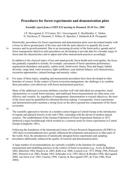
<strong>Procedures</strong> <strong>for</strong> <strong>for</strong>est <strong>experiments</strong> <strong>and</strong> <strong>demonstration</strong> <strong>plots</strong><br />
Scientific report from a COST E42 meeting in Denmark 28-30 Nov. 2006<br />
J.P. Skovsgaard, E. O’Connor, H.C. Graversgaard, E. Hochbichler, C. Mohni,<br />
N. Nicolescu, P. Niemistö, F. Pelleri, H. Spiecker, I. Stefancik & R. Övergaard<br />
Historically, procedures <strong>for</strong> <strong>for</strong>est <strong>experiments</strong> <strong>and</strong> <strong>demonstration</strong> <strong>plots</strong> were developed mainly with<br />
a focus on above-ground parts of the trees <strong>and</strong> with the main objective to quantify the wood<br />
resource <strong>and</strong> its growth potential. Due to an increasing diversity of the <strong>for</strong>est policy agenda <strong>and</strong> of<br />
<strong>for</strong>est management objectives plot procedures are developing to provide data <strong>for</strong> a broader range of<br />
<strong>for</strong>est <strong>and</strong> site characteristics <strong>and</strong> to adjust <strong>and</strong> refine measurement practices accordingly.<br />
In addition to the classical topics of tree <strong>and</strong> st<strong>and</strong> growth, <strong>for</strong>est health <strong>and</strong> wood quality, the focus<br />
has gradually exp<strong>and</strong>ed to include, <strong>for</strong> example, assessment of <strong>for</strong>est operations per<strong>for</strong>mance,<br />
regeneration abundance <strong>and</strong> quality, carbon stock, biodiversity (fauna, flora <strong>and</strong> fungi), habitat<br />
diversity, range l<strong>and</strong>, water resources, light conditions, crop nutrient balance, soil characteristics,<br />
recreation opportunities, cultural heritage <strong>and</strong> amenity values.<br />
For many of these topics, sampling <strong>and</strong> measurement procedures have been developed in other<br />
branches of science. In the context of <strong>for</strong>est ecosystem management, the challenge is to combine<br />
these procedures cost-effectively with <strong>for</strong>est measurement practices.<br />
Many of the additional ecosystem attributes correlate well with individual tree properties, st<strong>and</strong><br />
characteristics or overall <strong>for</strong>est structure, <strong>and</strong> traditional <strong>for</strong>est measurements are often more costeffective<br />
<strong>and</strong> versatile. So, regardless of management, <strong>demonstration</strong> or reseach objectives, the trees<br />
of the <strong>for</strong>est must be quantified <strong>for</strong> in<strong>for</strong>med decision making. Consequently, <strong>for</strong>est <strong>experiments</strong><br />
<strong>and</strong> <strong>demonstration</strong> <strong>plots</strong> maintain a strong focus on the above-ground tree components of the <strong>for</strong>est<br />
ecosystem.<br />
The scientific approach to <strong>for</strong>estry in a modern context began in Central Europe at the introduction<br />
of regular <strong>and</strong> planned <strong>for</strong>estry in the mid-1700s, coinciding with the advent of modern natural<br />
sciences. The establishment of the German Federation of Forest Experiment Stations in 1872<br />
furthered a major breakthrough which resulted in a common norm <strong>for</strong> <strong>for</strong>est <strong>experiments</strong> in Central<br />
Europe (Ganghofer 1881).<br />
Following the foundation of the International Union of Forest Research Organizations (IUFRO) in<br />
1892 these recommendations have greatly influenced developments <strong>and</strong> practices in other parts of<br />
the world. Next, the introduction of statistically-designed <strong>for</strong>est <strong>experiments</strong> <strong>and</strong> sampling<br />
procedures additionally enhanced the quality of research <strong>and</strong> <strong>demonstration</strong> <strong>plots</strong>.<br />
A large number of recommendations are currently available in the literature <strong>for</strong> sampling,<br />
measurement <strong>and</strong> modelling practices in the context of <strong>for</strong>est ecosystems (e.g., Avery & Burkhart<br />
2002, Bitterlich 1984, Husch et al. 2003, Köhl et al. 2006, Loetsch et al. 1973, Philip 1994, Pretzsch<br />
2001, Pretzsch et al. 2002, Prodan 1965, Schreuder et al. 1993, Shiver & Borders 1996, Skovsgaard<br />
2004, van Soest et al. 1965, Vanclay 1994, Vanclay & Skovsgaard 1997, de Vries 1986, West<br />
2004).
50<br />
60<br />
70<br />
80<br />
90<br />
<strong>Procedures</strong> <strong>for</strong> <strong>for</strong>est <strong>experiments</strong> <strong>and</strong> <strong>demonstration</strong> <strong>plots</strong> have received less comprehensive<br />
attention, <strong>and</strong> generally with little concern <strong>for</strong> practical matters which may influence the<br />
interpretation of observations (e.g., Alder & Synnott 1992, Condit 1998, Fabricius et al. 1936,<br />
Jeffers 1959, Johann 1993, Pretzsch 2002 – Henriksen 1961, + Res. Inst. Baden-Württemberg).<br />
The following recommendations <strong>for</strong> plot procedures summarise decades of practical experience in<br />
experimental silviculture. More attention is given to pragmatic solutions rather than <strong>for</strong>mal or<br />
statistical rigour. However, this should not detract from the fact that all experimentation in <strong>for</strong>estry<br />
should be basically be based on statistically-designed lay-out <strong>and</strong> sampling procedures.<br />
Considering the relevant research or demostration objectives, the intention throughout is to<br />
minimize costs relative to the expected output. To ensure that the initial investment of establishing<br />
research <strong>and</strong> <strong>demonstration</strong> <strong>plots</strong> is not lost, things which may go wrong during the investigation is<br />
given special attention.<br />
Research <strong>and</strong> <strong>demonstration</strong> objectives<br />
All <strong>experiments</strong> <strong>and</strong> <strong>demonstration</strong> <strong>plots</strong> should have a defined objective.<br />
The objective(s) should be associated with one or more testable hypotheses.<br />
Hypotheses should preferably relate to the underst<strong>and</strong>ing of cause-effect relationships.<br />
Decide on test criteria (test accuracy) as early as possible. Obviously, this relates to choice of<br />
variables, sampling intensity <strong>and</strong> measurement procedures.<br />
Consider the longeviety of the investigation.<br />
Often research or <strong>demonstration</strong> objectives may be viewed under different time constraints, <strong>for</strong><br />
example including short-, medium- <strong>and</strong> long-term objectives.<br />
Disregarding the type of research objective, all <strong>experiments</strong> should include <strong>demonstration</strong> options.<br />
Often, <strong>demonstration</strong> <strong>plots</strong> are directly oriented towards <strong>for</strong>estry practice <strong>and</strong> with the aim of<br />
demonstrating effects of two or more contrasting management practices within a relatively short<br />
period of time.<br />
Disregaring <strong>demonstration</strong> objective, all <strong>demonstration</strong> <strong>plots</strong> should include the option of<br />
statistically-based analyses.<br />
Treatments<br />
Experiments <strong>and</strong> <strong>demonstration</strong> <strong>plots</strong> should include contrasting treatments.<br />
Treatments should be objectively defined <strong>and</strong> preferably specified on a numerical basis.<br />
Avoid treatment specifications which are highly subjective or depending specifically on the<br />
personal view of one or more scientists, <strong>for</strong>est managers or l<strong>and</strong> owners.<br />
Simple specifications should be preferred over more complex treatments which, with the passage of<br />
time, may be difficult to repeat or interpret.<br />
Treatments should range beyond, but include, the range of contemporary, recommended (or<br />
prescribed) <strong>for</strong>estry practices, <strong>and</strong> preferably include one or more treatments which, at the time of<br />
establishement, are considered extreme compared to contemporary management practices.<br />
There are several objectives of including extreme treatments. One is provide a suitable basis <strong>for</strong><br />
interpolation (as it is undesirable to do extrapolation <strong>for</strong> treatments which, now or in the future, may<br />
be used in <strong>for</strong>estry practice). Another is that management practices may change considerably over<br />
time, thus changing the perception or relevance of extremes.<br />
2
100<br />
110<br />
120<br />
130<br />
140<br />
Statistical design<br />
In a designed experiment, all the variables are supposedly held constant except those varied<br />
according to the design. Hence, all variables are accounted <strong>for</strong>. Data collected without the aid of an<br />
experimental design may be suspect <strong>for</strong> a variety of reasons.<br />
Factorial design:<br />
One-factor <strong>experiments</strong><br />
R<strong>and</strong>omized block design<br />
Latin square design<br />
Factorial design<br />
Split-plot design<br />
Balanced <strong>and</strong> unbalanced incomplete block design<br />
Combination of <strong>experiments</strong> carried out on several sites <strong>and</strong> in different years<br />
Special designs (Nelder, CCT, Scots plaid, clinal) – those might be difficult to evaluate / interprete<br />
Mention advantages <strong>and</strong> drawbacks of each design. – See Marks Nester’s book on design etc.<br />
Placement of <strong>plots</strong><br />
Ideally, experimental <strong>plots</strong> should sample the geographic range over which results will be used, <strong>and</strong><br />
encompass the full range of <strong>for</strong>est types, site productivity <strong>and</strong> topography, which is considered to be<br />
relevant <strong>for</strong> the issue in question.<br />
Number of <strong>plots</strong><br />
The number of <strong>plots</strong> depends on the research objective <strong>and</strong> acceptable error of key variables, but is<br />
in practice often dictated by available l<strong>and</strong> area <strong>for</strong> each site <strong>and</strong> by the resources available. There is<br />
little point establishing more <strong>plots</strong> than can be maintained. It is better to have a few <strong>plots</strong> providing<br />
reliable data, than many <strong>plots</strong> with inadequate management. The number of <strong>plots</strong> should also be<br />
determined by the variability of the <strong>for</strong>est <strong>and</strong> the need to sample the full range of <strong>for</strong>est conditions.<br />
– Design the experiment in a cost-effective way.<br />
A database comprising a few <strong>plots</strong> each with many remeasurements violates statistical assumptions<br />
of independence, <strong>and</strong> may require special analyses (West et al. 1984, 1986, West 1994). This<br />
violation becomes significant when the number of remeasures is large relative to the number of<br />
<strong>plots</strong>. However, <strong>plots</strong> must be retained <strong>for</strong> extended periods with many remeasures to allow<br />
convincing tests <strong>and</strong> confidence in possible extrapolations.<br />
Within-site replicates<br />
Between-site replicates<br />
International cooperation<br />
Single-tree <strong>plots</strong><br />
The issue of co-variates – promote the use co-variates<br />
Genuine vs. pseudo-replications. For example, the potential of enlarging <strong>plots</strong> may be desirable if<br />
the experiment should continue longer than originally planned: This can be achieved if some<br />
neighbouring <strong>plots</strong> are treated identically or similarly according to one or more criteria. Again, the<br />
use of co-variates is important, - vs. r<strong>and</strong>omization.<br />
3
150<br />
160<br />
170<br />
180<br />
For area-based variables: Number of replicates should also depend on production risk. There should<br />
always be a minimum of two replicates, at least <strong>for</strong> the extreme treatments.<br />
The number of treatments should be balanced with the number of replications.<br />
For variables based on individual trees (or parts of trees): Use statistical <strong>for</strong>mulas.<br />
Within-site replication of treatments should be preferred over additional variations of treatments.<br />
If such additional variations are desired, <strong>for</strong> whatever reason, <strong>and</strong> the l<strong>and</strong> area available is<br />
insufficient, a compromise may be made by replicating a combination of highly relevant treatments<br />
<strong>and</strong> extreme treatments with unreplicated <strong>plots</strong> of treatment variations.<br />
Size <strong>and</strong> shape of <strong>plots</strong><br />
Size of <strong>plots</strong><br />
Minimum number of trees = 10 in final sample<br />
log Area = 5 - log N + 'research intensity factor' (red = 1, black = 3, blue = 5)<br />
Can we identify a 'universal' CV <strong>for</strong> important variables?<br />
What is the propability of (not) detecting a treatment effect if CV = 10% <strong>and</strong> N = 10?<br />
Shape of <strong>plots</strong>: Circular (small demo-<strong>plots</strong>), otherwise close to a square.<br />
Explain the idea of a modular approach. Start with full plot, but sample sub-<strong>plots</strong> within the full<br />
plot, subsequently exp<strong>and</strong> sample size or size of sample units.<br />
Buffer zone <strong>and</strong> plot surrounds<br />
Edge effects. - There must be a minimum size (relative to shape), considering edge effects. This<br />
must relate to tree height (equals ½-one tree height) - but a buffer zone of one tree height would<br />
dem<strong>and</strong> too large areas. – Find a compromise between replications, nett plot size <strong>and</strong> available l<strong>and</strong><br />
area. – The more serious the edge effect is expected to be, the wider the buffer zone.<br />
Include something on the single tree approach.<br />
Plot subdivisions<br />
Often stem mapping is not possible because of budget constraints.<br />
In this situation, plot subdivisions may provide an indication of spatial within-plot variations.<br />
Plot subdivisions can be established based on permanent plot demarcations.<br />
Plot subdivisions may be marked in the field at regular intervals by short pegs, nails or similar.<br />
4
Temporary markings (which may last <strong>for</strong> years) by nylon str<strong>and</strong>s (?).<br />
Planted st<strong>and</strong>s vs. naturally regenerated st<strong>and</strong>s.<br />
1<br />
10001<br />
Row -2<br />
Row 2<br />
Row 4<br />
Row 0<br />
Row 6<br />
1<br />
Row 9<br />
Row 11<br />
Row 13<br />
Row 16<br />
Row 18<br />
Row 20<br />
5<br />
400<br />
Field 1<br />
Field 2<br />
Field 3<br />
Field 4<br />
Field 5<br />
Figure<br />
Two examples showing plot subdivisions <strong>for</strong> a young planted st<strong>and</strong>.<br />
Above: nett plot. Below: gross plot, including buffer zone.<br />
Row 15<br />
Row 17<br />
Field 0<br />
Field 1<br />
Field 2<br />
Field 3<br />
Field 100
190<br />
200<br />
210<br />
Trns 1 Trns 2 Trns 3<br />
s - d - h - llb s - d - h - llb<br />
10 m<br />
6<br />
d<br />
+ (x,y,z)<br />
1.5 m<br />
Figure<br />
Example showing plot subdivision <strong>for</strong> a young naturally regenerated st<strong>and</strong> with four different<br />
measurement intensities. Red dots: permanently marked corner posts. Bold black dots: trees which<br />
are measured <strong>for</strong> status (dead/alive), diameter, height to lower live branch <strong>and</strong> total height. Bold<br />
gray dots: trees which are measured <strong>for</strong> status (dead/alive) <strong>and</strong> diameter.Thin black dots: trees<br />
which are not measured.<br />
A third alternative is, <strong>for</strong> example, circular <strong>plots</strong> within a full <strong>and</strong> fully treated plot.<br />
Plot demarcation <strong>and</strong> surveying<br />
GPS<br />
Mapping of the location.<br />
INKA-TINKA <strong>plots</strong>, mention those as an example.<br />
Permanent demarcation of plot corners <strong>and</strong> other permanent research areas (<strong>for</strong> biodiversity,<br />
photograpy, soil condition etc.). – Galvanized iron pipe.<br />
Trenches? - Do we still recommend trenches at plot corners? No, but the practice should be<br />
mentioned. – Plast markers agricultural cerials.<br />
Concrete corner beacons? - Can anybody af<strong>for</strong>d this?<br />
Identification <strong>and</strong> numbering of marker posts<br />
Visibility of markings (including plastic rods).<br />
Mapping of plot <strong>and</strong> tree locations.<br />
Marking of <strong>plots</strong>:<br />
Permanent markings cost little more than temporary markings.<br />
Corners or centre?<br />
Visible or invisible?
220<br />
230<br />
Invisible: There should be permanent markings in the field anyway, to be located based on mapped<br />
in<strong>for</strong>mation or gps <strong>and</strong> possibly metal detector.<br />
Visible: Always map the plot boundaries <strong>and</strong> plot surroundings, in case a machine, a log, a tourist<br />
(or otherwise) damages plot markings.<br />
20 m<br />
Trns 1 Trns 2 Trns 3<br />
+ ext. wood quality<br />
s -d -h -llb<br />
10 m<br />
Photo point<br />
40 m<br />
7<br />
d<br />
s -d -h -llb<br />
+ (x,y,z)<br />
Bio point<br />
1.5 m<br />
d + (x,y,z)<br />
Nett plot<br />
Gross plot<br />
Figure<br />
Example of fully marked, but yet extensively monitored young naturally regenerated st<strong>and</strong>.<br />
Figure<br />
Example of an intensively measured section of a stem mapped transsect in a young naturally<br />
regenerated st<strong>and</strong> of beech (cf. above).<br />
General visibility<br />
Marking of buffer zone
240<br />
250<br />
260<br />
270<br />
280<br />
Site assessment<br />
Including soil <strong>and</strong> other indicators (flora, fauna, fungi ?).<br />
L<strong>and</strong>-use history<br />
Site mapping (elevation, exposure, drainage etc).<br />
Soil pit combined with “stik” – <strong>for</strong> example 10 x 10 m<br />
Sampling procedures<br />
Define the statistical population<br />
Sampling methods:<br />
Unrestricted r<strong>and</strong>om sampling<br />
Stratified r<strong>and</strong>om sampling<br />
Subjective sampling<br />
Sequential sampling<br />
Point sampling<br />
Sampling <strong>for</strong> rare objects<br />
Shape <strong>and</strong> size of sampling unit<br />
Selection of sampling units<br />
Number of sample units required<br />
Uni<strong>for</strong>mity trials <strong>and</strong> pilot surveys<br />
The sampling scheme should consider the options <strong>for</strong> statistical analyses<br />
Measurement procedures<br />
Measurement intensity (<strong>and</strong> accuracy) should relate to research objective (<strong>for</strong> example, growth<br />
responses to st<strong>and</strong> treatment practices vs. variations in relative provenance per<strong>for</strong>mance). The<br />
expected response surface have implications <strong>for</strong> sampling <strong>and</strong> measurement procedures.<br />
Investigations which involve per area estimates vs. individual trees (<strong>for</strong> example, 'rare' admixed,<br />
valuable broadleaved tree species).<br />
Disragarding scale, admixed tree or individual tree management approaches should always be<br />
considered an integral part of st<strong>and</strong> management or the silvicultural system.<br />
What to measure - at initial measurement, on re-measurement occassions, at final measurement<br />
What to measure depending on budget. As annual budgets may vary considerably all measurement<br />
procedures <strong>for</strong> <strong>experiments</strong> <strong>and</strong> <strong>demonstration</strong> <strong>plots</strong> should include three levels of measurement<br />
intensity depending on available funds.<br />
Measurement size thresholds<br />
Tree numbering <strong>and</strong> marking:<br />
Paint<br />
Metal numbers<br />
Plastic numbers - two different types<br />
Electronic chips<br />
Numbering <strong>and</strong> marking of other measurement items<br />
Stem mapping<br />
Marking of potential crop trees<br />
8
290<br />
300<br />
Variables to measure<br />
Number of observations needed on each variable <strong>for</strong> the cv to stabilize<br />
Consider measurement error relative to rate of change to decide on when to remeasure<br />
Measurement scales:<br />
Nominal (categorical)<br />
Ordinal (rank)<br />
Interval (numerical without zero)<br />
Relative (numerical with zero)<br />
Stem mapping procedures – do a special discussion<br />
Instruments<br />
Regular checking of instruments<br />
Regular trainíng of staff <strong>and</strong> quality control<br />
We want consistent measurement st<strong>and</strong>ards.<br />
Refer to st<strong>and</strong>ard texts regarding classical <strong>for</strong>est mensuration, - but should we do something special<br />
<strong>for</strong> 'other' variables? - wood quality? - recreation? - where is the limit, <strong>and</strong> how do we strike a<br />
balance.<br />
Measuring exterior wood quality - an example<br />
Exterior wood quality variables<br />
Epicormics count<br />
Bend at 1.3 m<br />
Bend at 3.0 m<br />
Tilt at 6.0 m<br />
1.3 m<br />
6.0 m<br />
3.0 m<br />
9<br />
Lower live branch<br />
+ direction<br />
Forking height<br />
Transverse bending
320<br />
330<br />
340<br />
Exterior wood quality: the positives<br />
• No <strong>for</strong>king < 6 metres<br />
• High natural pruning<br />
• Vertical (no tilting)<br />
• Straight (no bending)<br />
• No epicormics<br />
• No or little transverse bending<br />
(sinousity)<br />
• No or little spiral grain<br />
• Regular spatial distribution<br />
310<br />
10<br />
Eight exterior wood quality variables<br />
• Vertical (no tilt)<br />
• Straight (no bend)<br />
• No <strong>for</strong>king < 6 metres<br />
• High natural pruning<br />
• No epicormics<br />
• No or little transverse<br />
bending (sinousity)<br />
• No or little spiral grain<br />
Data recording <strong>and</strong> processing<br />
Notebook<br />
Loose paper sheets – minimum requirements, provide examples<br />
Electronic data recording by entering data manually to field pc<br />
Direct electronic data recording to field pc<br />
Keeping track of individual instruments in case of errors relating to these<br />
Data quality control, in the field <strong>and</strong> subsequently<br />
Note the name of measuring crew<br />
When to measure <strong>and</strong> remeasure<br />
-<br />
Tilt at 6.0 m + direction<br />
Bend: 1.3 + 3.0 m + (0,1,2)<br />
Height to lowest <strong>for</strong>k<br />
Height to lower live branch<br />
No of epicormics < 6 m<br />
Present = 1, Absent = 0<br />
+ OS tree: dist + dir<br />
Establishment report<br />
Always make an establishment report including relevant in<strong>for</strong>mation on research or <strong>demonstration</strong><br />
objectives, location of experiment, statistical design, plot lay-out, plot demarcations, site conditions<br />
(climate, topography, soil), initial st<strong>and</strong> conditions, treatment specifications, measurement<br />
programme (three levels, depending on funding), status of experiment depending on funding,<br />
agreement on conditions <strong>for</strong> conduct of experiment signed by all partners involved (research<br />
institution, l<strong>and</strong> owner, <strong>for</strong>est authority <strong>and</strong> other relevant partners). – Including photographs.<br />
Administration<br />
Databases of <strong>for</strong>estry <strong>experiments</strong> (example: NOLTFOX, http://noltfox.metla.fi/).<br />
Priorities of <strong>experiments</strong> (institutional or otherwise)<br />
Searchable database of <strong>experiments</strong> <strong>and</strong> demo-<strong>plots</strong> at regional, national or super-national level, <strong>for</strong><br />
example in the context of a <strong>for</strong>est owners' association, a regional <strong>for</strong>est authority, a national <strong>for</strong>est<br />
service or a group of countries.<br />
Costs<br />
Generally, initial costs <strong>for</strong> planning <strong>and</strong> establishing an experiment are considerably higher than<br />
costs of remeasurement <strong>and</strong> maintenance.<br />
Overview of costs on a relative scale (rule-of-thumb, excluding travelling cost):<br />
Plot installment costs 100 Once<br />
Initial meauserement 100 Once
350<br />
360<br />
370<br />
380<br />
390<br />
Re-measurement 50 At regular, short intervals<br />
Plot maintenance 50 At regular, long intervals<br />
Final measurement 75 Once<br />
Plot maintenance<br />
Here we need lots of paint <strong>and</strong> students<br />
Regular reappraisal of <strong>experiments</strong> <strong>and</strong> <strong>demonstration</strong> <strong>plots</strong><br />
Research priorities<br />
Experiment priorities<br />
Measurement programmes depending on funding<br />
Special considerations depending on research or <strong>demonstration</strong> objective<br />
What do we do about valuable broadleaves?<br />
Can we define a st<strong>and</strong>ardized procedure <strong>for</strong> sparsely admixed trees, <strong>for</strong> example based on circular<br />
<strong>plots</strong> with a size depending on the size of the target tree? – Single-tree <strong>plots</strong>.<br />
Chronosequences <strong>and</strong> growth series (Wuchsreihe – Assmann; single-tree gowth series - Spiecker).<br />
In<strong>for</strong>mation to the public<br />
?<br />
Intellectual property rights<br />
Continuity – in funding (diferent funding scenarios), in objectives, in working methods,<br />
experimental infrastucture (who is doing what) ----- etc.<br />
Replicability – persuading, but all <strong>for</strong>estry acitivities will be (more or less) situational<br />
The notion of covariates vs. replicability<br />
Catalogue of irregularities<br />
Other items<br />
Can we make a simple check-list <strong>for</strong> general use? This would be very valuable.<br />
We should make a brief guideline, including site assessment <strong>and</strong> spread-sheet <strong>for</strong> measurements, <strong>for</strong><br />
use by <strong>for</strong>estry practice, simple research <strong>plots</strong> <strong>and</strong> inexperienced scientists.<br />
Publish interesting results<br />
Literature:<br />
Alder, D. & T.J. Synnott 1992: Permanent sample plot techniques <strong>for</strong> mixed tropical <strong>for</strong>est. Ox<strong>for</strong>d<br />
Forestry Institute, Tropical Forestry Papers, vol. 25. XI + 124 pp.<br />
Avery, T.E. & H.E. Burkhart 2002: Forest Measurements. McGrawHill. 5th ed. XXIII + 456 pp.<br />
Bitterlich, W. 1984: The Relascope Idea. Commonwealth Agricultural Bureau. XIV + 242 pp.<br />
Condit, R. 1998: Tropical <strong>for</strong>est census <strong>plots</strong>. Spinger. 211 pp.<br />
Fabricius, L., A. Oudin & W.H. Guillebaud 1936: Outlines <strong>for</strong> permanent sample plot<br />
investigations. International Union of Forest Research Organizations. Ox<strong>for</strong>d University<br />
Press. 32 pp.<br />
Ganghofer, A. (ed.) 1881: Das Forstliche Versuchswesen, Vol. 1. Augsburg. 504 pp.<br />
Husch, B., T.W. Beers & J.A. Kershaw 2003: Forest Mensuration. Wiley. 4th ed. 456 pp.<br />
11
400<br />
410<br />
420<br />
430<br />
Jeffers, J.N.R. 1959: Experimental design <strong>and</strong> analysis in <strong>for</strong>est research. Almqvist & Wiksell,<br />
Stockholm. 172 pp.<br />
Johann, K. 1993: DESER-Norm 1993. Normen der Sektion Ertragskunde im Deutschen Verb<strong>and</strong><br />
Forstlicher Forschungsanstalten zur Aufbearbeitung von waldwachstumskundlichen<br />
Dauerversuchen. Tagungsbericht von der Jahrestagung 1993 der Sektion Ertragskunde im<br />
Deutschen Verb<strong>and</strong> Forstlicher Forschungsanstalten in Unterreichenbach-Kapfenhardt, pp.<br />
96-104.<br />
Köhl, M., S.S. Magnussen & M. Marchetti 2006: Sampling methods, remote sensing <strong>and</strong> GIS<br />
multiresource <strong>for</strong>est inventory. Spinger. XIX+ 373 pp.<br />
Loetsch, F., F. Zöhrer & K.E. Haller 1973: Forest Inventory. Vol 2. BLV Verlagsgesellschaft,<br />
München, Bern, Wien. XXIV + 469 pp.<br />
Philip, M.S. 1994: Measuring Trees <strong>and</strong> Forests. CAB International. 2nd ed. XIV + 310 pp.<br />
Pretzsch, H. 2001: Modellierung des Waldwachstums. Parey (Blackwell), Berlin. XVI + 341 pp.<br />
Pretzsch, H. 2002: Grundlagen der Waldwachstums<strong>for</strong>schung. Parey (Blackwell), Berlin. XIV +<br />
414 pp.<br />
Pretzsch, H., P. Biber, J. Dursky, K. von Gadow, H. Hasenauer, G. Kändler, G. Kenk, E. Kublin, J.<br />
Nagel, T. Pukkala, J.P. Skovsgaard, R. Sodtke & H. Sterba 2002: Recommendations <strong>for</strong> the<br />
st<strong>and</strong>ardized documentation <strong>and</strong> further development of <strong>for</strong>est growth simulators.<br />
Forstwissenschaftliches Centralblatt 121: 138-151.<br />
Prodan, M. 1965: Holzmesslehre. J.D. Sauerländer's Verlag, Frankfurt am Main. XV + 644 pp.<br />
Schreuder, H.T., T.G. Gregoire & G.B. Wood 1993: Sampling Methods <strong>for</strong> Multiresource Forest<br />
Inventory. Wiley. XV + 446 pp.<br />
Shiver, B.D. & B.E. Borders 1996: Sampling techniques <strong>for</strong> <strong>for</strong>est resource inventory. Wiley. XII +<br />
356 pp.<br />
Skovsgaard, J.P. 2004: Forest measurements. Encyclopedia of Forest Sciences 3: 550-566.<br />
Skovsgaard, J.P., V.K. Johannsen & J.K. Vanclay 1998: Accuracy <strong>and</strong> precision of two laser<br />
dendrometers. Forestry 71: 131-139.<br />
van Soest, J., P. Ayral, R. Schober & F.C. Hummel 1965: The st<strong>and</strong>ardization of symbols in <strong>for</strong>est<br />
mensuration. International Union of Forestry Research Organizations. Approved by IUFRO<br />
1956, originally published 1959, <strong>and</strong> reprinted 1965 by University of Maine as Technical<br />
Bulletin no. 15 of Maine Agricultural Experiment Station. 32 pp.<br />
Vanclay, J.K. 1994: Modelling <strong>for</strong>est growth <strong>and</strong> yield. CAB International. XVII + 312 pp.<br />
Vanclay, J.K. & J.P. Skovsgaard 1997: Evaluating <strong>for</strong>est growth models. Ecological Modelling 98:<br />
1-12.<br />
Vanclay, J.K., J.P. Skovsgaard & C.P. Hansen 1995: Assessing the quality of permanent sample<br />
plot databases <strong>for</strong> growth <strong>and</strong> yield modelling in <strong>for</strong>est plantations. Forest Ecology <strong>and</strong><br />
Management 71: 177-186.<br />
de Vries, P.G. 1986: Sampling theory <strong>for</strong> <strong>for</strong>est inventory. Springer-Verlag. X + 399 pp.<br />
West, P.W. 2004: Tree <strong>and</strong> <strong>for</strong>est measurement. Springer. XII + 167 pp.<br />
Bannwaldaufnahme<br />
12


