Marriage and Money: Variations across the Earnings ... - UQ eSpace

Perry Australian & Wilson: Journal of The Labour Accord Economics, and Strikes Vol. 8, No. 2, June 2005, pp 163 - 179163Marriage and Money: Variationsacross the Earnings DistributionMark WesternUniversity of Queensland Social Research Centre &Sociology, School of Social ScienceThe University of QueenslandBelinda HewittSociology, School of Social ScienceThe University of QueenslandJaneen BaxterSociology, School of Social ScienceThe University of QueenslandAbstractThis paper uses Australian data from the Negotiating the Life Course Project 1997to investigate the impact of marriage on men’s and women’s earnings. We extendearlier earnings research and investigate whether the effect of marriage is constantfor men and women at different points on the conditional earnings distribution byusing robust and quantile regression techniques. We find no association betweenmarriage and wages for women, but for men a large and significant premium existswith married men earning around $5,700 per annum more than their unmarriedcounterparts, after adjusting for human capital, job and family characteristics.Overall, there are very few differences in the association between marriage andearnings for men and women across the wage distribution. Although, importantly,we find that the returns to marriage tend to be smaller and non-significant formen at the top of the distribution than for men in the middle of the distribution.1. IntroductionPrevious research has consistently found that married men earn more thansingle men (Gray, 1997; Korenman and Neumark, 1991; Loh, 1996; Blackburnand Korenman, 1994; Chalmers, 2002; Hill, 1979). Moreover, the higherearnings of married men persist even when differences in education, labourmarket experience, occupational and demographic characteristics arecontrolled. The general consensus is that, controlling for observablecharacteristics, married men are more productive than unmarried men(Chalmers, 2002; Daniel, 1995; Gray, 1997).Two main explanations for the productivity of married men have emerged.The specialisation argument is that married men are more productive inAddress for correspondence: Associate Professor Mark Western, UQSRC and TheSchool of Social Science, The University of Queensland, St Lucia Qld 4072 Australia.Email: m.western@uq.edu.auWe would like to thank members of the Negotiating the Life Course project, JennyChesters and anonymous reviewers for comments on earlier versions of this paper.© Centre for Labour Market Research, 2005

164Australian Journal of Labour Economics, June 2005the labour market due to role specialisation in households. In marriedhouseholds women specialize in domestic duties and men specialize in thelabour market, enabling married men to be more productive at work thanunmarried men. The second explanation is that there are selection effectswhereby the unobservable characteristics of men that are valued in themarriage market are also valued in the labour market. Under this scenariomen who are successful in the labour market are also more likely to marry.While evidence has been found for both explanations, on balance, theavailable research tends to favour specialisation with the gender divisionof labour in the household allowing a married man the time and energy topursue labour market goals (Becker, 1985; Blackburn and Korenman, 1994;Chalmers, 2002; Gray, 1997; Korenman and Neumark, 1991; Loh, 1996).For women, the relationship between marriage and earnings is morecomplex. The findings of previous studies have been mixed, and sometimescontradictory (Budig and England, 2001; Dolton and Makepeace, 1987;Goldin and Polachek, 1987; Gray, 1997; Hill, 1979; Waldfogel, 1997). Earlyresearch investigating the relationship between marriage and women’searnings found little or no association (Dolton and Makepeace, 1987; Goldinand Polachek, 1987; Hill, 1979), whereas more recent studies, usinglongitudinal data, have found significant positive associations (Budig andEngland, 2001; Waldfogel, 1997). Moreover, studies investigating thedeterminants of women’s earnings tend to find a significant wage penaltyfor motherhood, where mothers earn less than non-mothers, rather than astrong association between marriage and earnings (Budig and England,2001; Harkness and Waldfogel, 1999; Korenman and Neumark, 1992;Waldfogel, 1997). The evidence suggests then that marriage may increasewomen’s earnings, but this pattern is strongly counter-balanced by thenegative impact of motherhood.Despite the burgeoning literature examining the association betweenmarriage and earnings, especially for men, very little is known about theassociation between marriage and earnings at varying points on thedistribution. In this study we investigate the relationship between marriageand earnings for both men and women. We extend earlier research bycomparing the effect of marriage at different points on the earningsdistribution using quantile regression methods. This is important becauseboth the specialisation and selection hypotheses can be qualified to implydifferent marriage premiums depending on where on the incomedistribution we examine the relationship.2. The Marriage Premium for MenThere are several reasons to believe that the association between earningsand marriage for men may differ depending on where they are situatedwithin the earnings distribution. For instance, if specialisation benefits arethe primary mechanism for the association between marriage and earningsfor men one might expect similar returns to marriage for men at all pointson the distribution. Feminist research has long recognised the‘incorporation’ of wives into husbands’ work and the importance of theirrole as providers of domestic labour, emotional support and in some cases,

Western, Hewitt & Baxter: Marriage and Money: Variations across theEarnings Distribution165a direct contribution to the husbands job through a range of essential, butunpaid activities, such as entertaining clients, secretarial work and accountkeeping(Finch, 1983; Delphy and Leonard, 1992). In Married to the Job Finchargues that this kind of incorporation is not restricted to wives ofprofessional workers, but rather extends across the occupational structureto include wives of those employed in services, trades and manual work.In arguing for specialisation effects associated with marriage, Daniel (1995)came up with the term augmentation capital to describe the ability of a wifeto enhance her husband’s productivity in the work place by providing aflow of services ranging from organising activities, running errands,performing housework, and other household chores. He argues that evenwhen a woman marries a man with lower earnings, she is still likely tohave augmentation capital and provide her husband with a marriagepremium (Daniel, 1995: 119). Under this scenario returns to marriage wouldbe expected to differ depending on the degree of specialisation within thehousehold. However, since augmentation capital contributes directly tomen’s productivity we can also qualify the standard specialisation argumentto anticipate larger premiums at the top of the earnings distribution than atthe middle or bottom. If, as human capital theory argues, earnings reflectmarginal productivity, we can think about augmentation capital asenhancing the marginal productivity of the ‘last’ married employee, relativeto the ‘last’ nonmarried employee. Enhanced marginal productivityassociated with augmentation capital may arise because married men havemore time to devote to paid work than single men, are able to commit morefully to it in other ways (such as psychologically or emotionally), or havegreater flexibility with respect to paid work than single men, so that theyare better able to adjust to changing work demands. In all these cases though,we might expect that the additional ‘effort’ married men are able to makein paid work by comparison to single men translates into a larger premiumat the top of the earnings distribution, either because it does genuinelyimply a greater difference in the marginal productivity of married and singlemen in highly paid jobs, compared to those in lower paid jobs, or because itis associated with employers’ perceptions of greater productivitydifferences. Differences in effort between those in highly paid jobs are likelyto be associated with larger earnings differentials than similar differencesin effort among those in lower paid jobs because productivity differences(real or perceived) are larger in the former case. We refer to this as theearnings enhanced specialisation argument, in contrast to the standardspecialisation argument, which implies a constant premium across theearnings distribution.If selection factors are the primary force underlying the marriage premium,one might also expect that men at the top of the earnings distribution wouldhave a larger premium than men at the lower end because men who earnmore money are more likely to be married (Becker, 1981). Prior studiesprovide evidence for this scenario. For example, Nakosteen and Zimmer(1997), using the 1979, 1982 and 1984 waves of the Panel Study on IncomeDynamics investigated the probability of marriage for single men who hadabove average earnings and found that those with higher than expected

166Australian Journal of Labour Economics, June 2005earnings were significantly more likely to marry within the study timeframe. Selectivity implies that unmeasured characteristics that are valuablefor both marriage and employment explain the marriage premium for men.The likely mechanism here is that employers use marriage as an indicatorof other desirable characteristics that employees possess. In highly paidjobs, being unmarried may therefore carry a greater ‘penalty’ since it signalsthe absence of such characteristics more strongly in a pool where a higherproportion of men are married. We describe this as the earnings enhancedselection effect to contrast it against the standard selection argument of aconstant marriage premium.3. Marriage and Women’s EarningsEarly research examining the determinants of women’s earnings found thatmarriage had little or no association once adjustments were made for humancapital (education, work experience, tenure), job characteristics (hoursworked, occupation, employment conditions), and family status (thepresence or number of children). For example, Hill (1979) using data fromthe 1976 Panel Study of Income Dynamics found no significant associationbetween marriage and wages. Controlling for education, work experienceand number of children, her results show that married, white women earnmore than unmarried women, but less than divorced, separated or widowedwomen. Dolton and Makepeace (1987) also found no association betweenmarriage and wages among female college graduates. Goldin and Polachek(1987), on the other hand, using 1980 U.S. Census data found that singlewomen had a wage advantage over married women, but these differenceswere small once adjustments were made for variability in expected levelsof accumulated human capital.More recent investigations have focused specifically on the wage penaltyfor motherhood. Budig and England (2001) used the National LongitudinalSurvey for Youth, 1982-1993, and adjusting for a wide range of humancapital, family, and job characteristics, found a marriage premium forwomen of around 4 per cent. They also found that being divorced, separated,and widowed had a large positive effect on women’s earnings comparedto being married or never married. Waldfogel (1997) also found a marriagepremium for women, but found that divorced, separated and widowedwomen had higher earnings than both married and never married women.A possible explanation for the consistent finding across both studies thatwomen who are divorced, separated, and widowed usually have higherwages than married women is that previously married women move intothe workforce out of economic necessity when they experience the loss oftheir partner, whereas they otherwise may not (Waldfogel, 1997).Taken together this evidence suggests that the relationship betweenmarriage and women’s earnings appears to be changing. While earlierresearch found little, or no, association between marriage and earnings,recent studies have found significant positive associations. There are severalpossible explanations for this shift. First, there have been major socialchanges for women since the 1970s, such as increased participation in highereducation and employment, which may have led to a shift in thedeterminants of female earnings. Secondly, studies show that male earnings

Western, Hewitt & Baxter: Marriage and Money: Variations across theEarnings Distribution167have declined over the last few decades, whereas female earnings haveincreased (England, 2001; Oppenheimer, 1997). This reduction in maleearnings relative to female earnings may encourage men to select partnerswho are able to make economic contributions to the family, therebygenerating a selection effect for women who have earnings potential intomarriage. On the other hand, the observed change in the relationshipbetween marriage and wages for women could be attributable to differencesin statistical methods. Korenman and Neumark (1992) criticized the use ofcross-sectional techniques in examining the relationships between marriage,motherhood and wages for women for underestimating the effects of thesedeterminants on wages.In addition to expecting an association between marriage and earnings forwomen, there are several scenarios under which one might expect theassociation between women’s earnings and marriage to differ dependingon where they are situated within the earnings distribution. Under thespecialisation argument women would be expected to experience a negativereturn to marriage across all levels of the earnings distribution due to thenegative impact of housework duties on women’s wages. While recentresearch into household specialisation indicates that in households wherewomen work full-time the division of household labour is more egalitarian(Bianchi et al., 2000), women still do more domestic labour overall and aremore likely to adjust their working arrangements to accommodate demandsfrom home (Western and Baxter, 2001). Therefore, women who work parttimeare more likely to spend more time and energy on domestic tasks(Baxter, 1991) and face a wage penalty from marriage. On the other hand,women who are employed full-time may have a smaller marriage penaltybecause they are more likely to be in households where the division of labouris more equal, and they are better able to pursue labour market goals. Underthe standard specialisation argument, we would expect the marriage penaltyto be consistent across the earnings distribution for both full and part-timeemployed women, but smaller for full-time women than part-time women.Unlike for men, there is no earnings-enhanced specialisation effect.With regard to selectivity, the increase in women’s labour force involvementand earnings potential, relative to men’s reduced earnings potential(Oppenheimer, 1997; England, 2001), may predispose men to select wiveswho have high earnings, or potential for high earnings as marriage partners.South (1991) has found that men take into consideration their prospectivepartner’s employment potential when deciding whether to marry. Underan earnings-enhanced selection scenario the marriage premium would workin the same way for women as for men, with women at the top end of theearnings distribution experiencing a larger marriage premium than womenat the lower end of the distribution. Further this would apply irrespectiveof whether the woman works full or part-time, because even if a woman isworking part-time she may make a more attractive spouse if she can earn ahigher income in the time she works.The above arguments suggest that effects of specialisation and selectionare much more complex for women than for men. As indicated earlierspecialisation acts primarily to men’s advantage and to women’sdisadvantage in relation to earnings. Therefore, the act of specialisation

168Australian Journal of Labour Economics, June 2005operates to limit women’s earnings potential. Given this, women selectedinto marriage on their earnings potential will also have a reduced likelihoodof realising that potential, compared to women who do not marry, becauseof the disadvantages associated with specialisation within marriage. Forexample, for women, unlike men, the potential marriage premium due toselection may be counter-balanced by the overall negative impact ofdomestic work and motherhood resulting in a small or zero return tomarriage for women at the upper ends of the earnings distribution and apenalty for women at the lower ends if they have children. Some evidenceexists for this possibility in the research literature. Budig and England (2001)found an interaction effect between marriage and children, with the size ofthe marriage premium declining as the number of children in the householdincreased so that by three children, there was actually a wage penalty formarriage.In summary, research examining the association between marriage andearnings focuses on the selection or specialisation debate for men, and thewage penalty to motherhood for women. Within these literatures no studiesto date have investigated the association between marriage and earningsacross the distribution, even though there are clear theoretical reasons fordoing so. We develop the earnings enhanced selection and specialisationarguments for men, and the earnings enhanced selection argument forwomen to take account of these possibilities. We examine these ideasempirically using the Negotiating the Life Course survey 1997. First weexamine the nature and extent of the effects of marriage on earnings,emphasising differences both between the sexes, and between individualsaccording to marital status. Second we investigate the relationship betweenmarriage and earnings at different points on the conditional distribution,rather than simply focusing on the mean.4. MethodsAnalytical SampleThe data used in this paper come from the Negotiating the Life Course1997, Version 1 (McDonald et al., 2000). For the current analyses we restrictthe sample to men and women who were employed at the time of survey.Respondents who are on paid maternity or ‘other’ leave, such as sick orlong service leave, are included. The self-employed are excluded. Therewere 1298 respondents in the final analytic sample.VariablesThe dependent and independent variables are described in Appendix 1.Summary statistics for all variables are shown in Table 1. The dependentvariable is gross (i.e. before tax) annual earnings. While a measure of hourlywage rates may be preferable for testing the effect of marriage on earnings,we are restricted here to examining annual earnings because data were notcollected on number of weeks worked each year. We are therefore unableto accurately estimate hourly wage rates for respondents. We focus on rawearnings rather than logged earnings because the arguments about thedifferent size of the marriage premium at different points on the earningdistribution relate to absolute differences rather than percentage differences.

Western, Hewitt & Baxter: Marriage and Money: Variations across theEarnings Distribution169The primary independent variable, marital status, consists of a series ofdummy variables for never married, previously married (divorced,separated, and widowed) and currently married or cohabiting, 1 with nevermarried as the reference group.Table 1 Means and Standard Deviations for all VariablesMen Full-time Women Full-time Women Part-time(N=583) (N=422) (N=293)Mean SD Mean SD Mean SDAnnual Earnings 45535.81 35816 33509.73 15148 13848.01 8909Married .65 .57 .66Ever Married .09 .16 .14Never Married .26 .27 .20Age 36.50 9.0 35.86 9.8 36.40 9.9Years of Education 14.98 3.3 14.93 3.2 13.88 3.2Degree or better (1=yes) .25 .30 .16Missing education (1=yes) .02 .02 .05Years of Work Experience a 18.86 9.2 14.96 8.0 11.17 6.4Pre-school child (1=yes) .21 .09 .23No Children .50 .61 .28One Child .15 .16 .23Two Children .23 .18 .31Three, or more Children .12 .05 .18Private Sector .73 .61 .71Government Sector .27 .39 .29Managerial Occupation .12 .04 .01Professional Occupation .34 .47 .29White Collar Occupation .14 .39 .54Blue Collar Occupation .38 .08 .15Missing Occupation .02 .02 .01a. Because age and work experience are highly correlated we orthogonalised themby using residualised experience from an OLS regression of experience on age forinclusion in the models.Human capital is measured by variables for age, education and workexperience. We fit linear and quadratic terms for age. We use two educationmeasures, a continuous variable for years of education constructed usingretrospective education life history data from the age of 15, and a level ofeducation variable to estimate years of schooling before the age of 15. Wealso include dummy variables for university bachelor degree or higher andmissing values for education in some models. We construct a measure foractual years of work experience using retrospective life history data collectedfrom the age of 15, and incorporating years of part-time and full-timeexperience, with years of part-time experience weighted to 0.5.This study uses two measures of family status: a series of dummy variablesfor number of children in the household including, no children, one child,1Cohabiting unmarried couples are included with married couples in this analysisas we were interested in the presence, or not, of a partner within the household.There are studies that have found qualitative differences between registeredmarriages and defacto unions in relation to the marriage premium (i.e. Brown andBooth, 1996; Nock, 1995). Further, there is some evidence that there is an associationbetween cohabitation and a decline in the marriage premium for men (Cohen, 2002).However, we did not have an adequate sample size to address differences betweenmarried and cohabiting respondents here.

170Australian Journal of Labour Economics, June 2005two children, and three or more children, with no children as the referencegroup; and a dummy variable for whether or not a pre-school child is presentin the household, because the presence of younger children in the householdhas been found to influence women’s earnings (Harkness and Waldfogel,1999).Finally we include measures of job characteristics. We include a measurefor occupation based on major occupational categories 2 of the AustralianStandard Classification of Occupations (ASCO), second edition (AustralianBureau of Statistics, 1997). We collapse these into four categories: (1)managers and administrators, (2) professionals, (3) white collar employees,(4) and blue collar workers. Managers and administrators are the referencecategory. We also include a dummy variable for missing responses onoccupation, and a dummy variable for whether or not the respondent wasa government employee.AnalysesTo examine the marriage premium we fit five robust regression and quantileregression models to separate samples of full-time male and femaleemployees and part-time female employees. We pursue separate analysesbecause earnings determination processes differ across the three groups(Harkness and Waldfogel, 1999; Waldfogel, 1997). We use robust regressionbased on iterative reweighted least squares to model the conditional meanearnings in each group, and simultaneous bootstrapped quantile regressionsof the deciles (10 th , 20 th , 30 th etc. to 90 th percentiles) to model other points onthe distribution. The five analytic models include a baseline modelincorporating marital status only, a second model that adds the humancapital variables (age, education and experience), and a third model thatadds job characteristics. Model 4 is the second model plus family variables(numbers of children and the presence/absence of preschool children), andModel 5 includes all variables (marital status, human capital, family, andjob characteristics). This staged procedure allows us to examine how themarriage premium changes as we introduce human capital and othervariables that previous research has found to be differentially related tothe earnings of women and men (Hill, 1979).We use a robust estimator for the mean, rather than conventional OLSbecause preliminary analyses using OLS revealed the presence of variousinfluential data points and outliers. 3 The IRLS estimator starts with an OLSfit and uses Cook’s distances to identify extreme observations. It then runsiterative reweighted least squares, initially weighting observations using aHuber function and then Tukey’s biweight until convergence (Hamilton,2002; Stata Corporation, 2001:152-157). The bootstrapped quantile regressionestimator minimises a sum of weighted absolute deviations based on the2The Australian Standard Classification of Occupations (ASCO) is a skill-basedmeasure that groups together occupations requiring similar levels of education,knowledge, responsibility, and on-the-job training and experience. The occupationalgroupings are hierarchically ordered based on their relative skill-levels, with thoseoccupations having the most extensive skill requirements located at the top of thehierarchy (ABS, 1997). The nine-level ASCO classification comprises Managers andAdministrators, Professionals, Associate Professionals, Trades and Related, AdvancedClerical, Intermediate Clerical, Intermediate Production and Transport, ElementaryClerical, and labour and Related.3Influential observations were identified by looking at leverage values, Cook’sdistances, studentised residuals and DFBETAs from OLS runs.

Western, Hewitt & Baxter: Marriage and Money: Variations across theEarnings Distribution171relevant quantile, while bootstrap resampling (Davison and Hinkley, 1997)is used to generate the estimated variance-covariance matrix of parameterestimates (Stata Corporation, 2001:11-27). The analyses are based on 1000bootstrap resamples.5. ResultsTable 2 presents results of the robust regression models. For ease ofpresentation we only show coefficients for the marital status dummyvariables. The baseline model shows that full-time employed men has asignificant marriage premium of around $12,800 per annum, compared tonever married men, and that men who were previously married earn justover $6,000 per annum more than never married men. Adding human capitalvariables, as shown in Model 2, attenuates the return to marriage for menby around half to just over $7,000 per annum. The association betweenpreviously (ever) married men and earnings becomes smaller and nonsignificantwith the introduction of human capital factors, and remains nonsignificantfor all other models. The R-squared also increases substantially(from 0.10 to 0.27) with the introduction of human capital factors andincreases marginally again with the introduction of the job variables. 4Adjusting for job characteristics (Model 3) and family status (Model 4), inaddition to human capital factors does not have a significant effect on wagesfor married men. The final model includes human capital, job characteristicsand family status variables; after adjusting for all variables married menearn around $5,700 per annum more than single men. Thus, about 55 percent of the male full-time marriage premium is accounted for by controllingfor human capital, family and job variables ((12779-5701)/12779 * 100 = 55.4).Table 2 Marital Status Dummy Coefficients for Robust Regression ModelsM3: M4:Baseline, Baseline,M2: Human HumanM1: Baseline Capital & Capital & M5:Baseline & Human Job Charact- Family AllModel Capital eristics Status VariablesFull-time Employed MenMarried 12779.32 ** 7215.79 ** 5888.90 ** 7498.08 ** 5701.94 **Ever Married 6337.75 * 2465.68 2232.53 2505.25 2152.30Never Married - - - - -Observations 583 583 583 583 583R-squared .10 .25 .34 .26 .34Full-time Employed WomenMarried 2750.29 * 439.27 -238.63 850.53 156.80Ever Married 4264.65 * 2128.05 1543.90 2638.72 2190.75Never Married - - - - -Observations 422 422 422 422 422R-squared .01 .34 .39 .34 .39Part-time Employed WomenMarried 3378.77 * 240.63 -1489.21 1150.61 -304.64Ever Married 4430.12 * 1090.76 713.72 1898.35 1744.66Never Married - - - - -Observations 293 293 293 293 293R-squared .03 .10 .19 .12 .20*P

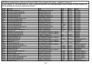
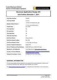
172Australian Journal of Labour Economics, June 2005In contrast to results for men, there is generally no significant associationbetween marriage and the earnings of women employed full-time. Thisfinding supports earlier research using cross sectional data (Dolton andMakepeace, 1987; Hill, 1979; Korenman and Neumark, 1992). A smallpremium for previously (ever) married women disappears once humancapital differences are controlled. For women employed part-time, however,the baseline model (Model 1) indicates a large significant associationbetween marriage and earnings, where both currently and ever marriedwomen have higher earnings per annum than never married women. Again,however, these differences are fully accounted for by human capitaldifferences in married and single women. After controlling for age,education and experience, there are no significant associations betweenmarriage and wages for part-time employed women in the remaining fourmodels (Models 2-5).Consistent with earlier studies, our results thus show a significant positiveassociation between marriage and men’s average earnings. For women therelationship between marriage and earnings tends to be small and nonsignificantafter adjusting for compositional differences in human capital.This is again consistent with previous cross-sectional studies using OLS(Dolton and Makepeace, 1987; Hill, 1979; Korenman and Neumark, 1992).Studies examining the determinants of women’s earnings more often findthat motherhood, has a stronger influence on women’s earnings thanmarriage, being associated with a substantial wage penalty (Budig andEngland, 2001; Waldfogel, 1997). Models 4 and 5 include dummy variablesfor the number of children, and presence of a pre-school child, but our results(not shown) do not provide support for a wage penalty for motherhood foreither full-time or part-time women. As expected none of the family statusvariables were significantly associated with men’s wages either.To further investigate the relationship between marriage and earnings wenext estimate quantile regression models for the conditional deciles. Figures1-3 present graphs of the quantile regression coefficients for the final modelsseparately for each of the three subsamples. In each figure, the first graphshows the conditional quantile regression coefficients for marriedrespondents compared to never married ones, and the next graph showsthe coefficients for those ‘ever previously married’ (separated, divorced,widowed) compared to never married. For brevity we only present resultsfrom the final model. For all graphs, the solid line represents the robustregression estimate (i.e. the relevant dummy variable coefficient from therobust regression model), the dotted line is the conditional quantileregression coefficient at each of the nine deciles, and the dashed lines arethe upper and lower pointwise confidence limits for the quantile coefficients.Where the confidence band incorporates zero the relationship betweenmarriage and earnings are not statistically significant. The figures also enableus to see how closely the robust coefficient tracks the quantile coefficientsalong the earning distribution.

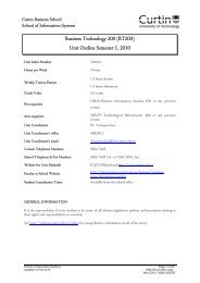
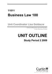
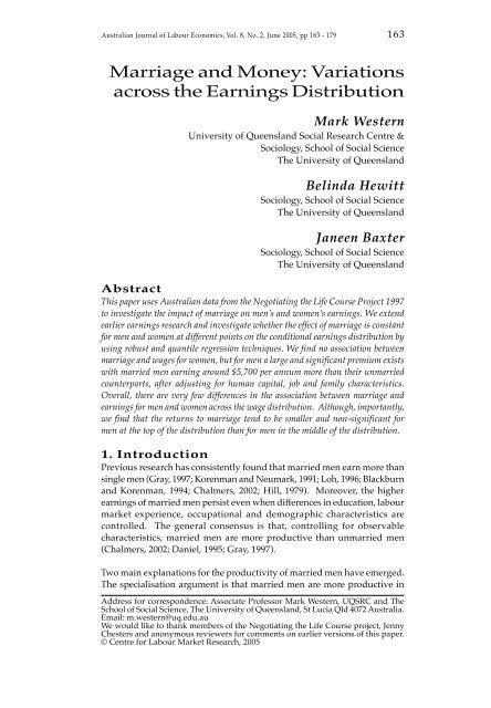
174Australian Journal of Labour Economics, June 2005Figure 2 Final Model Full-time Employed WomenFigure 3 presents results for women employed part-time. The robustregression is also a good predictor of the relationship between marriageand earnings for part-time employed women of different income levels.These results further suggest that part-time women tend to have a largerearnings return to marriage than full-time women, but generally therelationship is not significant. Overall, the quantile regressions support thefindings of the robust regressions, showing virtually no association betweenmarriage and earnings for women irrespective of the amount they earned.Figure 3 Final Model Part-time Employed Women

Western, Hewitt & Baxter: Marriage and Money: Variations across theEarnings Distribution1756. DiscussionOur examination of the relationship between earnings and marriage showa large and significant marriage premium for men, but little or no associationbetween marriage and earnings for women. Adjusting for a range of humancapital, job, and family characteristics married men in our study earn around$5700 more per annum, on average, than unmarried men. These findingssupport the findings of previous studies examining the determinants ofearnings for men, and other cross-sectional studies on the determinants ofwomen’s earnings (Blackburn and Korenman, 1994; Dolton and Makepeace,1987; Gray, 1997; Hill, 1979; Korenman and Neumark, 1991; Korenman andNeumark, 1992). One possible explanation for the lack of associationbetween marriage, family and earnings for women in our study is our useof cross-sectional data. Other studies have found some limitations withusing cross-sectional data to examine determinants of women’s earnings,because they tend to under-estimate the effects of marriage and family(Korenman and Neumark, 1992). Previous studies that found significantassociations between marriage and women’s incomes tended to belongitudinal (Budig and England, 2001; Korenman and Neumark, 1992;Walfogel, 1997). Alternatively our lack of findings of any effects for marriagefor women could be attributable to joint processes of selection andspecialisation whereby women’s earnings are limited by specialisation evenif they are selected into marriage because of their earnings potential, therebycancelling out any differences at the mean.Most significantly, our study extends the existing literature to examine therelationship between marriage and earnings for men and women situatedat different levels on the earnings distribution. Overall, we found that theeffects of marriage are similar for men and women irrespective of wherethey are situated on the wage distribution, however, the quantile regressionresults do provide additional insight into the relationship.For men, the effect of marriage on earnings is different at the extreme endsof the distribution but not in the manner predicted by either the earningsenhanced specialisation or selection hypotheses. In contrast to predictions,men who are at the higher end of the earnings distribution do not have thesame large and significant benefits associated with marriage as men in themiddle of the wage distribution. For men at the lower end of the distributionthe effects are of a similar magnitude as middle-income men, but theassociation is not significant. These findings do not provide unequivocalsupport for a selection or specialisation argument. Having said that,however, the full model for married men (Figure 1) shows a pattern ofassociation across the distribution that is fairly consistent with a standardspecialisation argument. Here the returns to marriage are virtually the samefor men at the second to eighth deciles. The standard and modifiedspecialisation arguments, however, do not hold for married men at theextreme high-end of the earnings distribution, those around the 9 th decile,who have small and non-significant returns to marriage compared to menin the middle of the distribution. This finding is also in contrast to theexpected association between marriage and earnings for a selectionargument, where high earnings men should have a larger return to marriage.This finding is consistent with other theories, such as economic rent theory.An economic rent exists where payment is made for access to economic

176Australian Journal of Labour Economics, June 2005resources in fixed supply, and persons with ownership of, or effective controlover the economic resource have possession of the right to the payment(Sorensen, 1996; Sorensen, 2000). Two kinds of employment rents arerelevant to our findings. First, monopoly rents exist where employees areable to demand, and/or employers are willing to pay salaries above thecompetitive wage rate for certain skills, talents or abilities possessed byindividuals that are in short supply (Sorensen, 1996). Monopoly rents applyparticularly to professional occupations that are credentialised so that onlyworkers with specialized knowledge and formal qualifications can accessthe occupation. This creates scarcity that drives up the price of professionallabour. Second, loyalty rents, or efficiency wages, may also be paid to thosein administrative and managerial positions. Management andadministration positions are difficult for employers to regulate so a wageabove the competitive wage rate is offered to buy loyalty, and increaseincentives to perform (Bowles and Gintis, 1990). A substantial componentof the earnings of men with high earnings may reflect these types of rentswhich are associated with the nature of the job position, rather thancharacteristics of the individual such as marital status, and human capital.Under this scenario one would expect that the returns to marriage wouldbe lower for men as they move up the earnings distribution, because otherwage determinants become more important.There is some indication of employment rent processes in our results. Inthe final, full regression model we find that none of the human capitalcharacteristics (i.e. education, work experience) are significant for men atthe 9 th decile, whereas human capital is associated with earnings for men atall other deciles. Other than age the only significant factors for men in the9 th decile are job characteristics; the dummy for white collar employee (-0.40), and the dummy for public sector employment (-0.17), both had largenegative coefficients (results not shown). These results are consistent withthe existence of employment rents in highly paid managerial and privatesector jobs for full-time male employees. Alternatively, for men at the topof the earnings distribution, earnings may less adequately represent thebenefits associated with work. This may be because we do not use a morecomprehensive measure of compensation, including performance pay,allowances and the like, might have shown a premium for this group ofmen.For women, in general, the relationship between earnings and marriagewas small and non-significant. Contrary to our expectations, there is noassociation between marriage and earnings for women irrespective ofwhether they have children, or work full or part-time.In addition to the substantive issues above, the quantile regressions enabledus to compare the effectiveness of using a statistical technique that uses theconditional mean function of the wage distribution with one that examinesthe relationship at several points on the conditional distribution. In mostcases we find that the robust regressions adequately predict the effects ofmarriage on wages across the entire earnings distribution.More broadly our results also offer some insight into the continuing gendergap in earnings (Cotter et al., 1995; Le and Miller, 2001; Wellington, 1994).While there is no evidence here to suggest that being married is necessarily

Western, Hewitt & Baxter: Marriage and Money: Variations across theEarnings Distribution177a disadvantage for women’s earnings, they certainly do not receive thepremium for marriage that men do. It is therefore not unreasonable toconclude that the persistence of the gender wage gap is due at least in part,to differential returns to marriage for men and women. Additionally, ourfindings indicate that men situated at the upper end of the earningsdistribution have diminished returns to marriage than men lower in thedistribution, and may therefore have different earnings mechanismsoperating. This result indicates that further research is required thatexamines the determinants of earnings for men at different levels of income,rather than simply focusing on the mean, to develop our understanding ofthe relationship between marriage and earnings for men. Given our results,selection and specialisation effects for men are not enhanced at the top ofthe distribution, as we expected. Rather, the implication is that the selectionand specialisation mechanisms associated with marriage are offset by otherfactors that determine the earnings of highly paid men. This suggests thatwe need to think further about appropriately qualified variants of thespecialisation and selection hypotheses when examining the male marriagepremium.Appendix 1 Description of VariablesVariablesDependent:Annual EarningsPrimary Independent:MarriedEver MarriedNever MarriedHuman Capital:AgeAge#2Years of EducationDegree or betterYears Work ExperienceYears Work Experience#2Family Status:Pre-school childNo ChildrenOne ChildTwo ChildrenThree, or more ChildrenJob Characteristics:Government SectorManagerial OccupationProfessional OccupationWhite Collar OccupationBlue Collar OccupationDefinition of VariableGross annual income, loggedDummy variable for people in married or defacto relationships(1=Married, defacto)Dummy variable for people who were previously married(1=Divorced, Separated or Widowed)Dummy for people who have never been married (ReferenceCategory)Age of respondentAge of respondent centred and squared to adjust for non-linearrelationship with wagesContinuous measure of years of education of respondent,incorporates level of education measure and retrospective datafrom age of 15 years, retrospective component includes years offull-time and part-time study weighted by 0.5.Dummy for if respondent has bachelor degree or higher(1=Bachelor degree)Continuous measure of years of work experience, includes fulltime years of work, and part-time years of work weighted by0.5. Residualized with age so work experience is net of theinfluence of age.Yrs Work Experience residualized, centred and squared.Dummy for the presence of a preschool aged child in house(1=preschool child present)Dummy for No children in Household (Reference Group)Dummy for One child in Household (1=1 Child)Dummy for Two children in Household (1=2 Children)Dummy for Three or more children in Household(1=3 or more Children)Dummy for Government or Private sector (1=Government)(Reference group)Dummy for professional occupation (1=Professional, associateprofessional)Dummy for White collar employee (1=Sales, Service, Clerical)Dummy for Blue Collar employee (1=Trades, Labourer)

178Australian Journal of Labour Economics, June 2005ReferencesAustralian Bureau of Statistics (ABS), 1997, Australian Standard Classificationof Occupations, Cat No. 1220.0.Baxter, J. (1991), Work at Home: The Domestic Division of Labour, Universitof Queensland Press.Becker, G.S. (1981), A Treatise on the Family, Cambridge, MA, HarvardUniversity Press.Becker, G.S. (1985), ‘Human Capital Effort, and the Sexual Division ofLabour’, Journal of Labour Economics, 3, S33-S58.Bianchi, S., Milkie, M., Sayer, L. and Robinson, J. (2000), ‘Is Anyone Doingthe Housework? Trends in the Gender Division of HouseholdLabour’, Social Forces, 79, 191-228.Blackburn, M. and Korenman, S. (1994), ‘The Declining Marital-statusEarnings Differential’, Journal of Population Economics, 7, 247-270.Bowles, S and Gintis, H. (1990), ‘Contested Exchange: NewMicrofoundations for the Political Economy of Capitalism’, Politicsand Society, 18, 165-222.Brown, S.L and Booth, A. (1996), ‘Cohabiting Versus Marriage: AComparison of Relationship Quality’, Journal of Marriage and theFamily, 58, 668-678.Budig, M.J. and England, P. (2001), ‘The Wage Penalty for Motherhood’,American Sociological Review, 66, 204-225.Chalmers, J. (2002), Why Marry? An Economic Analysis of the Male MarriagePremium, Unpublished PhD Thesis, Australian National University.Cohen, P.N. (2002), ‘Cohabitation and the Declining Marriage Premiumfor Men’, Work and Occupations, 29, 346-363.Cotter, D.A., DeFiore, J.M., Hermsen, J.M., Kowalewski, B.M., anVanneman, R. (1995), ‘Occupational Gender Segregation and theEarnings Gap: Changes in the 1980s’, Social Science Research, 24, 439-454.Daniel, K. (1995), ‘The Marriage Premium’, in Tommasi, M. and Ierulli, K.(ed.), The New Economics of Human Behaviour, 13-125,CambridgeUniversity Press.Davison, A.C. and Hinkley, D.V. (1997), Bootstrap Methods and theirApplication, Cambridge: Cambridge University Press.Delphy, C. and Leonard, D. (1992), Familiar Exploitation, A New Analysis ofMarriage in Contemporary Western Societies, London, Polity.Dolton, P.J. and Makepeace, G.H. (1987), ‘Marital Status, Child Rearing andEarnings Differentials in the Graduate Labour Market’, The EconomicJournal, 97, 987-922.England, P. (2001), ‘Gender and Access to Money: What do Trends inEarnings and Household Poverty Tell Us?’, 131-153, in Baxter, J. andWestern, M. (eds), Reconfigurations of Class and Gender, StanfordUniversity Press.Finch, J. (1983), Married to the Job. Wives’ Incorporation in Men’s Work, London,Allen and Unwin.Goldin, C. and Polachek, S. (1987), ‘Residual Differences by Sex: Perspectiveon the Gender Gap in Earnings’, The American Economic Review, 77,143-151.Gray, J.S. (1997), ‘The Fall in Men’s Return to Marriage’, The Journal of HumanResources, 32, 481-504.

Western, Hewitt & Baxter: Marriage and Money: Variations across theEarnings Distribution179Harkness, S. and Waldfogel, J. (1999), The Family Gap in Pay: Evidence fromSeven Industrialised Countries, Luxemburg Income Study, WorkingPaper No. 219.Hill, Martha S. (1979), ‘The Wage Effects of Marital Status and Children’,The Journal of Human Resources, 14, 579-594.Hamilton, L.C. (2002), Statistics with Stata: Updated for Version 7, Duxbury.Korenman, S. and Neumark, D. (1991), ‘Does Marriage Really MakeMen More Productive?’ The Journal of Human Resources, 26, 282-307.Korenman, S. and Neumark, D. (1992), ‘Marriage, Motherhood, and Wages’,The Journal of Human Resources, 27, 233-255.Le, A.T. and Miller, P.W. (2002), ‘The Persistence of the Female WageDisadvantage’, The Australian Economic Review, 34, 33-52.Loh, E.S. (1996), ‘Productivity Differences and the Marriage Wage Premiumfor White Males’, The Journal of Human Resources, 31, 566-589.McDonald, P., Jones, F., Mitchell, D. and Baxter, J. (2000a), Negotiating theLife Course, 1997 [computer file]. Canberra: Social Science DataArchives (SSDA), The Australian National University.McDonald, P., Evans, A., Baxter, J. and Gray, E. (2000b), ‘The Negotiating theLifecourse Survey Experience: implications for HILDA’, Unpublishedpaper presented at the Panel Data and Policy Conference, Australia,Canberra 1-3 May.Nakosteen, R. and Zimmer, M. (1997), ‘Men, Money and Marriage: Are HighEarners More Prone Than Low Earners to Marry?’, Social ScienceQuarterly, 78, 66-82.Nock, S.L. (1995), ‘A Comparison of Marriages and CohabitingRelationships’, Journal of Family Issues, 16, 53-76.Oppenheimer, V.K. (1997), ‘Women’s Employment and the Gain to Marriage:The Specialization and Trading Model’, Annual Review of Sociology,23, 431-453.Sorensen, A. (1996), ‘The Structural Basis of Social Inequality’, AmericanJournal of Sociology, 101, 1333-65.Sorensen, A. (2000), ‘Toward a Sounder Basis for Class Analysis’, AmericanJournal of Sociology, 105, 1523-58.South, S.J. (1991), ‘Sociodemographic Differentials in Mate SelectionPreferences’, Journal of Marriage and the Family, 53, 928-940.Stata Corporation, (2001), Stata Statistical Data Analysis, Version 7, 3, CollegeStation TX, Stata Corporation.Waldfogel, J. (1997), ‘The Effect of Children on Women’s Wages’, AmericanSociological Review, 62, 209-217.Wellington, A.J. (1994), ‘Accounting for the Male/Female Wage Gap AmoWhites: 1976 and 1985’, American Sociological Review, 59, 839-848.Western, M. and Baxter, J. (2001), ‘The Links between Paid and UnpaidWork: Australia and Sweden in the 1980s and 1990s’, 81-104 in Baxter,J. and Western, M. (eds), Reconfigurations of Class and Gender, StanfordUniversity Press.