graphics with PSTric..

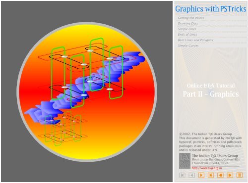
Graphics with PSTricksGetting the pointsDrawing DotsSimple LinesEnds of LinesBent Lines and PolygonsT T T E T E T X E E X E X E X X and and and and and and GraphicsGraphicsGraphicsGraphicsGraphicsSimple CurvesOnline L A T E X TutorialPart II – Graphicsc○2002, The Indian T E X Users GroupThis document is generated by PDFT E X withhyperref, pstricks, pdftricks and pdfscreenpackages in an intel PC running GNU/LINUXand is released under LPPLThe Indian T E X Users GroupFloor iii, sjp Buildings, Cotton HillsTrivandrum 695014, indiahttp://www.tug.org.in

Getting the pointsDrawing DotsSimple LinesEnds of Lines1. Graphics with PSTricksBent Lines and PolygonsSimple CurvesL A T E X has only limited drawing capabilities, while PostScript is a page descriptionlanguage which has a rich set of drawing commands; and thereare programs (such as dvips) which translate the dvi output to PostScript.So, the natural question is whether one can include PostScript code in a T E Xsource file itself for programs such as dvips to process after the T E X compilation?This is the idea behind the PSTricks package of Timothy van Zandt.The beauty of it is one need not know PostScript to use it—the necessaryPostScript code can be generated by T E X macros defined in the package.Online L A T E X TutorialPart II – Graphicsc○2002, The Indian T E X Users GroupThis document is generated by PDFT E X withhyperref, pstricks, pdftricks and pdfscreenpackages in an intel PC running GNU/LINUXand is released under LPPLThe Indian T E X Users GroupFloor iii, sjp Buildings, Cotton HillsTrivandrum 695014, indiahttp://www.tug.org.in

1.1. Getting the pointsAny picture is drawn by stringing together appropriate points. How do wespecify the points we need? We’ve a method of specifying each point ina plane using a pair of numbers, thanks to the 17 th century French mathematiciansPierre de Fermat and René Descartes. The method is to fix apair of perpendicular lines (called axes) and label each point with the numbersrepresenting its distance from these two points (called coordinates) asshown in the figure below:Graphics with PSTricksGetting the pointsDrawing DotsSimple LinesEnds of LinesBent Lines and PolygonsSimple Curves(0,0)3 unit(1.5,0.5)(3,2)2 unitOnline L A T E X TutorialPart II – GraphicsNote that the meeting point of the axes (called the origin) has coordinates(0,0). In order to associate each pair of numbers with a unique point, wemake the convention that horizontal distances to the left of the origin andvertical distances below the origin are negative as illustrated below:c○2002, The Indian T E X Users GroupThis document is generated by PDFT E X withhyperref, pstricks, pdftricks and pdfscreenpackages in an intel PC running GNU/LINUXand is released under LPPLThe Indian T E X Users GroupFloor iii, sjp Buildings, Cotton HillsTrivandrum 695014, indiahttp://www.tug.org.in

(-2,1)(-1,-1)(0,0)(2,-2)(3,2)Graphics with PSTricksGetting the pointsDrawing DotsSimple LinesEnds of LinesBent Lines and PolygonsSimple CurvesAnother fact to note is that the coordinates of points depend on theposition of the axes chosen, so that the same point has different pairs ofcoordinates with respect to different set of axes. This is illustrated in thefigure below, where the point which originally had coordinates (3,2) withrespect to the axes shown in gray has new coordinates (1,1) with respect tonew axes shown in black.Online L A T E X TutorialPart II – Graphics(0,0)(0,0)(1,1)(3,2)c○2002, The Indian T E X Users GroupThis document is generated by PDFT E X withhyperref, pstricks, pdftricks and pdfscreenpackages in an intel PC running GNU/LINUXand is released under LPPLThe Indian T E X Users GroupFloor iii, sjp Buildings, Cotton HillsTrivandrum 695014, indiahttp://www.tug.org.in

Graphics with PSTricksThe PSTricks package uses coordinates to specify points to plot and thenvarious other commands to join them.Getting the pointsDrawing DotsSimple LinesEnds of LinesBent Lines and PolygonsSimple CurvesOnline L A T E X TutorialPart II – Graphicsc○2002, The Indian T E X Users GroupThis document is generated by PDFT E X withhyperref, pstricks, pdftricks and pdfscreenpackages in an intel PC running GNU/LINUXand is released under LPPLThe Indian T E X Users GroupFloor iii, sjp Buildings, Cotton HillsTrivandrum 695014, indiahttp://www.tug.org.in

1.2. Drawing DotsNow let’s see how to draw pictures with PSTricks. The basic package touse is pstricks and so we assume in all the codes given below that thispackage has been loaded with the command \usepackage{pstricks} inthe document preamble.Let’s start with the simplest of graphical objects—a single dot. Type inthe code below in your document:Graphics with PSTricksGetting the pointsDrawing DotsSimple LinesEnds of LinesBent Lines and PolygonsSimple CurvesLook at this dot \psdots(1,0)and T E X compile the document. To produce the PostScript, you’ll have touse the dvips program or any other dvi to PostScript translator available inyour system. With dvips, this done by the commanddvips filename -owhere filename is the name of your file without any extension (or with theextension .dvi). This creates a PostScript file of the same name but withthe extension .ps which you can view using a PostScript previewer, such asghostview. It looks like this:Online L A T E X TutorialPart II – GraphicsLook at this dotSome explanations are in order. Evidently the command to draw a dotis \psdots followed by the coordinates of the point where the dot is to beplaced. But we know that the assignment of coordinates to points (and viceversa) makes sense only after fixing the axes. So when we specify coordinatessuch as (0,1) as above, what are the axes used? By default, PSTricksuses the current point in T E X as the origin and horizontal and vertical linesthrough this point as the axes. Again, the default unit is 1 cm. Thus in theabove example, a point is drawn 1 cm. away from the letter t in dot. This isc○2002, The Indian T E X Users GroupThis document is generated by PDFT E X withhyperref, pstricks, pdftricks and pdfscreenpackages in an intel PC running GNU/LINUXand is released under LPPLThe Indian T E X Users GroupFloor iii, sjp Buildings, Cotton HillsTrivandrum 695014, indiahttp://www.tug.org.in

Graphics with PSTricksillustrated in the figure below, where the (invisible) axes are shown in gray.Look at this dot 1 cm.(0,0)¡(1,0)Getting the pointsDrawing DotsSimple LinesEnds of LinesBent Lines and PolygonsSimple CurvesA single \psdots command can be used to plot any number of points.For example, the inputLook at these dots \psdots(0,0)(2,0)(1,1)produce the (PostScript) outputLook at these dotsOnline L A T E X TutorialPart II – GraphicsNow suppose we tryLook at these dots \psdots(0,0)(2,0)(1,1) forming the vertices(corners) of a triangle.the output produced isLook at these dots forming the vertexes (corners) of a triangle.What happened? Why were the dots overwritten? What happened actuallyis that T E X did not reserve any space for the picture (recall that thec○2002, The Indian T E X Users GroupThis document is generated by PDFT E X withhyperref, pstricks, pdftricks and pdfscreenpackages in an intel PC running GNU/LINUXand is released under LPPLThe Indian T E X Users GroupFloor iii, sjp Buildings, Cotton HillsTrivandrum 695014, indiahttp://www.tug.org.in

picture is drawn after the T E X compilation) and so the dots were drawn overthe text. (if you look closely, you can see that the dots are over the letters).This brings up an important point to be kept in mind: most of the PSTrickscommands produce 0-dimensional boxes in T E X. So, we must ensure that T E Xleaves enough space for the pictures to be drawn, by enclosing the picturein a T E X box of suitable size. PSTricks itself provides a convenient methodof doing this, in the form of the pspicture environment. See how we canmodify the previous example:Graphics with PSTricksGetting the pointsDrawing DotsSimple LinesEnds of LinesBent Lines and PolygonsSimple Curves\begin{pspicture}(-0.5,0)(2.5,1)\psdots(0,0)(2,0)(1,1)\end{pspicture}This gives the outputOnline L A T E X TutorialPart II – GraphicsHere the pairs (-0.5,0) and (2.5,1) are the coordinates of the bottom-leftand top-right corners of a box which encloses the picture as shown in thefigure below:Look at these dots(2.5,1)(–0.5,0)¡¡forming the vertexes of a triangle.In fact, the first pair of coordinates is optional and defaults to (0,0). Thusfor example,...c○2002, The Indian T E X Users GroupThis document is generated by PDFT E X withhyperref, pstricks, pdftricks and pdfscreenpackages in an intel PC running GNU/LINUXand is released under LPPLThe Indian T E X Users GroupFloor iii, sjp Buildings, Cotton HillsTrivandrum 695014, indiahttp://www.tug.org.in

Graphics with PSTricks\begin{pspicture}(1,2)...\end{pspicture}is equivalent to\begin{pspicture}(0,0)(1,2) ... \end{pspicture}Getting the pointsDrawing DotsSimple LinesEnds of LinesBent Lines and PolygonsSimple CurvesWe can also ‘display’ the picture by\begin{pspicture}(-0.5,-0.5)(2.5,1.5)\psdots(0,0)(2,0)(1,1)\end{pspicture}This producesCan you see why the second coordinate of the ‘box’ is changed to -0.5and 1.5 from its values 0 and 1 in the previous example?The dots we’ve been drawing so far are all circular and black. How aboutsquare and white dots? Change the input of the previous example as follows:Look at these dots\begin{center}\begin{pspicture}(-0.5,-0.5)(2.5,1.5)\psdots[dotstyle=square](0,0)(2,0)(1,1)\end{pspicture}\end{center}forming the vertices of a triangle.Online L A T E X TutorialPart II – Graphicsc○2002, The Indian T E X Users GroupThis document is generated by PDFT E X withhyperref, pstricks, pdftricks and pdfscreenpackages in an intel PC running GNU/LINUXand is released under LPPLThe Indian T E X Users GroupFloor iii, sjp Buildings, Cotton HillsTrivandrum 695014, indiahttp://www.tug.org.in

We then get the output shown below:Look at these dots¡forming the vertexes of a triangle.Thus the shape of the dots is controlled by the parameter dotstyle andit’s to be specified within square brackets after the \psdots command. Thevarious possible values of this parameter and the corresponding shape ofthe dots is shown in the table below:¡style example style example* o+ + + + x × × ×oplus ⊕ ⊕ ⊕ otimes ⊗ ⊗ ⊗asterisk* * *triangle£¤£¤£¤triangle*| | | |Graphics with PSTricksGetting the pointsDrawing DotsSimple LinesEnds of LinesBent Lines and PolygonsSimple CurvesOnline L A T E X TutorialPart II – Graphicssquare¦§¦§¦§square*¨diamond ♦ ♦ ♦ diamond* ◊ ◊ ◊pentagon©©©pentagon*Also, dots can be scaled using the parameter dotscale and rotated usingthe parameter dotangle. For example¥ ¡¢¡¢¡¢c○2002, The Indian T E X Users GroupThis document is generated by PDFT E X withhyperref, pstricks, pdftricks and pdfscreenpackages in an intel PC running GNU/LINUXand is released under LPPLThe Indian T E X Users GroupFloor iii, sjp Buildings, Cotton HillsTrivandrum 695014, indiahttp://www.tug.org.in

Graphics with PSTricks\begin{pspicture}(-0.5,-0.5)(2.5,2.5)\psdots[dotstyle=+,dotangle=45](0,0)\psdots[dotstyle=+,dotscale=1.5,dotangle=45](0.5,0.5)\psdots[dotstyle=+,dotscale=2,dotangle=45](1,1)\psdots[dotstyle=+,dotscale=2.5,dotangle=45](1.5,1.5)\psdots[dotstyle=+,dotscale=3,dotangle=45](2,2)\end{pspicture}Getting the pointsDrawing DotsSimple LinesEnds of LinesBent Lines and PolygonsSimple Curvesgives+ + +++Instead of scaling, we can explicitly specify the size of dots. But this we’lldiscuss in the next section (with a reason, of course).Online L A T E X TutorialPart II – Graphicsc○2002, The Indian T E X Users GroupThis document is generated by PDFT E X withhyperref, pstricks, pdftricks and pdfscreenpackages in an intel PC running GNU/LINUXand is released under LPPLThe Indian T E X Users GroupFloor iii, sjp Buildings, Cotton HillsTrivandrum 695014, indiahttp://www.tug.org.in

1.3. Simple LinesLet’s see how we draw lines next. The command is \psline with the coordinatesof the points to be joined. For exampleLook at the line segment below\begin{center}\begin{pspicture}(0,0)(3.5,2.5)\psline(2,1)(3,2)\end{pspicture}\end{center}equally slanted to the horizontal and the vertical.Graphics with PSTricksGetting the pointsDrawing DotsSimple LinesEnds of LinesBent Lines and PolygonsSimple CurvesgivesLook at the line segment belowOnline L A T E X TutorialPart II – Graphicsequally slanted to the horizontal and the vertical.We can draw dashed or dotted lines using the linestyle parameter.Thus\begin{pspicture}(0,0)(2,1)\psline(0,0)(2,0)\psline[linestyle=dashed](2,0)(1,1)\psline[linestyle=dotted](1,1)(0,0)\end{pspicture}givesc○2002, The Indian T E X Users GroupThis document is generated by PDFT E X withhyperref, pstricks, pdftricks and pdfscreenpackages in an intel PC running GNU/LINUXand is released under LPPLThe Indian T E X Users GroupFloor iii, sjp Buildings, Cotton HillsTrivandrum 695014, indiahttp://www.tug.org.in

Graphics with PSTricks100 1 2In this and many of the pictures below, we include a “coordinate grid” forconvenience of reference. It is not produced by the code given alongside.In the dashed style, the length of the black and white segments is controlledby the parameter dash Thus dash=3pt 2pt produces dashed linewith black segments of length 3 pt. and white segments of length 2 pt. Thus\begin{center}\begin{pspicture}(-0.5,-0.5)(2.5,1.5)\psline[linestyle=dashed,dash=2pt 2pt](0,0)(2,0)\psline[linestyle=dashed,dash=2pt 5pt](2,0)(1,1)\psline[linestyle=dashed,dash=5pt 5pt](1,1)(0,0)\end{pspicture}\end{center}Getting the pointsDrawing DotsSimple LinesEnds of LinesBent Lines and PolygonsSimple CurvesOnline L A T E X TutorialPart II – Graphicsgives100 1 2The default value of dash is 5 pt 3 pt. Again, in the dotted style, thedistance between dots is controlled by the parameter dotsep whose defaultvalue is 3 pt.We can also alter the thickness of the lines by changing the value ofthe parameter linewidth which has a default value of 0.8 pt. Look at theexample below:c○2002, The Indian T E X Users GroupThis document is generated by PDFT E X withhyperref, pstricks, pdftricks and pdfscreenpackages in an intel PC running GNU/LINUXand is released under LPPLThe Indian T E X Users GroupFloor iii, sjp Buildings, Cotton HillsTrivandrum 695014, indiahttp://www.tug.org.in

Graphics with PSTricks\begin{center}\begin{pspicture}(0,-0.5)(2.5,4.5)\psline[linewidth=0.2pt](0,0)(0,2)\psline[linewidth=0.4pt](0.5,0)(0.5,2)\psline[linewidth=0.6pt](1,0)(1,2)\psline[linewidth=0.8pt](1.5,0)(1.5,2)\psline[linewidth=1pt](2,0)(2,2)\psline[linewidth=1.2pt](2.5,0)(2.5,2)\psline[linewidth=1.4pt](3,0)(3,2)\psline[linewidth=1.6pt](3.5,0)(3.5,2)\psline[linewidth=1.8pt](4,0)(4,2)\psline[linewidth=2pt](4.5,0)(4.5,2)\end{pspicture}\end{center}Getting the pointsDrawing DotsSimple LinesEnds of LinesBent Lines and PolygonsSimple CurvesproducesOnline L A T E X TutorialPart II – Graphicsc○2002, The Indian T E X Users GroupThis document is generated by PDFT E X withhyperref, pstricks, pdftricks and pdfscreenpackages in an intel PC running GNU/LINUXand is released under LPPLThe Indian T E X Users GroupFloor iii, sjp Buildings, Cotton HillsTrivandrum 695014, indiahttp://www.tug.org.in

1.4. Ends of LinesLines can be provided with arrowheads. This is done by the arrows parameter\begin{center}\begin{pspicture}(0,-0.5)(2,2.5)\psline[arrows=->](0,0)(1,2)\psline[arrows=](1,1)(2,1)\end{pspicture}\end{center}Graphics with PSTricksGetting the pointsDrawing DotsSimple LinesEnds of LinesBent Lines and PolygonsSimple CurvesproducesInstead of arrowheads, lines can be made to terminate with circles, T-barsand so on, using the parameter arrows. The available values of this parameterand the corresponding line terminators are given in the Table 1.1. Wecan mix and match these terminators as values for the arrows parametersuch as *-> or |-

Graphics with PSTricksvalue example name- none arrowheads>-< reverse arrowheads double arrowheads>>-

Graphics with PSTricks\begin{pspicture}(-0.5,-0.5)(3.5,2.5)\psline[linewidth=0.5cm](0,0)(0,2)\psline[linewidth=0.5cm,arrows=c-c](1,0)(1,2)\psline[linewidth=0.5cm,arrows=cc-cc](2,0)(2,2)\psline[linewidth=0.5cm,arrows=C-C](3,0)(3,2)\end{pspicture}Getting the pointsDrawing DotsSimple LinesEnds of LinesBent Lines and PolygonsSimple CurvesgivesThe arrows parameter can also be specified as an optional argumentwithin braces after the other options (in square brackets). Thus instead ofOnline L A T E X TutorialPart II – Graphics\psline[linestyle=dotted,arrows=](0,0)(2,0)we can also write\psline[linestyle=dotted]{}(0,0)(2,0)Now is the time to talk of (no, not cabbages and kings) the size of dots.The diameter of a circular dot is 2.5 times the current linewidth plus .5 pt.This can be changed by the parameter dotsize. Thus for examplec○2002, The Indian T E X Users GroupThis document is generated by PDFT E X withhyperref, pstricks, pdftricks and pdfscreenpackages in an intel PC running GNU/LINUXand is released under LPPLThe Indian T E X Users GroupFloor iii, sjp Buildings, Cotton HillsTrivandrum 695014, indiahttp://www.tug.org.in

Graphics with PSTricks\begin{center}\begin{pspicture}(0,0)(2,2)\psdot[linewidth=0.1cm,dotsize=1cm 10](1,1)\end{pspicture}\end{center}Getting the pointsDrawing DotsSimple LinesEnds of LinesBent Lines and PolygonsSimple Curvesgiveswhich is a circular disk of diameters 10 × 0.1 + 1 = 2 centimeters. (We’llsoon see better method of drawing such disks). The polygonal dots aresized to have the same area as circles. The dotsize is made to depend onlinewidth since dots are often used in conjunction with lines as in arrows(and showpoints which we will discuss later). Note that the dotsize can beset to any absolute value independent of the linewidth by setting the secondnumber of the dotsize parameter to 0.There are parameters determining the dimensions of the other types ofline terminators also, which are given in Table 1.2. In this, width refers to adimension perpendicular to the line and length refers to a dimension in thedirection of the line.The example below illustrates the use of some of these parametersOnline L A T E X TutorialPart II – Graphicsc○2002, The Indian T E X Users GroupThis document is generated by PDFT E X withhyperref, pstricks, pdftricks and pdfscreenpackages in an intel PC running GNU/LINUXand is released under LPPLThe Indian T E X Users GroupFloor iii, sjp Buildings, Cotton HillsTrivandrum 695014, indiahttp://www.tug.org.in

parameter value descriptiondotsize = dim numtbarsize = dim numbracketlength = numrbracketlength = numnum × linewidth + dimnum × linewidth + dimnumber × widthnumber × widththe diameterof a circle ordiscthe width of aT-bar, squarebracket orround bracketthe lengthof a squarebracketthe length of around bracketTable 1.2: Parameters for line terminators\begin{center}\begin{pspicture}(-1,-1)(9,4)\psline[tbarsize=1cm 0,bracketlength=0.5]{[-|}(0,0)(3,0)\psline[tbarsize=1cm 0]{[-|}(0,3)(3,3)\psline[tbarsize=1cm 0,rbracketlength=0.5]{(-|}(5,0)(8,0)\psline[tbarsize=1cm 0]{(-|}(5,3)(8,3)\end{pspicture}\end{center}defaultvalue0.5 pt 52 pt 50.150.15Graphics with PSTricksGetting the pointsDrawing DotsSimple LinesEnds of LinesBent Lines and PolygonsSimple CurvesOnline L A T E X TutorialPart II – Graphicswhich produces the output below.c○2002, The Indian T E X Users GroupThis document is generated by PDFT E X withhyperref, pstricks, pdftricks and pdfscreenpackages in an intel PC running GNU/LINUXand is released under LPPLThe Indian T E X Users GroupFloor iii, sjp Buildings, Cotton HillsTrivandrum 695014, indiahttp://www.tug.org.in

Graphics with PSTricks4321Getting the pointsDrawing DotsSimple LinesEnds of LinesBent Lines and PolygonsSimple Curves0-1-1 0 1 2 3 4 5 6 7 8 9Note that the coordinate grid in the picture above is not produced by thegiven code.The shape of arrowheads is determined by its length, width and insetand the parameters controlling them are arrowsize, arrowlength andarrowinset as shown in the figure below:Online L A T E X TutorialPart II – Graphicslengthwidthinsetarrowsize = dim numwidth = num × linewidth + dimlength = arrowlength × widthinset = arrowinset × lengthc○2002, The Indian T E X Users GroupThis document is generated by PDFT E X withhyperref, pstricks, pdftricks and pdfscreenpackages in an intel PC running GNU/LINUXand is released under LPPLThe Indian T E X Users GroupFloor iii, sjp Buildings, Cotton HillsTrivandrum 695014, indiahttp://www.tug.org.in

Graphics with PSTricksThe default values of the parameters arearrowsize = 2 pt 3 arrowlength = 1.4 arrowinset = 0.4The example below illustrates the effect of changing these parameters.\begin{center}\begin{pspicture}(0.5,0.5)(5.5,4.5)\psline[linewidth=2pt,arrowsize=2pt 2,arrowlength=5,arrowinset=0.1]{->}(1,1)(4,4)\psline[linewidth=2pt]{->}(2,1)(5,4)\end{pspicture}\end{center}Getting the pointsDrawing DotsSimple LinesEnds of LinesBent Lines and PolygonsSimple CurvesOnline L A T E X TutorialPart II – GraphicsWe can also draw “double lines” by setting the parameter doubleline totrue (by default, it’s false). For example\begin{center}\begin{pspicture}(-0.5,-0.5)(2.5,2.5)\psline[linewidth=0.06,doubleline=true,doublesep=0.05,(0,0)(2,2)\end{pspicture}\end{center}c○2002, The Indian T E X Users GroupThis document is generated by PDFT E X withhyperref, pstricks, pdftricks and pdfscreenpackages in an intel PC running GNU/LINUXand is released under LPPLThe Indian T E X Users GroupFloor iii, sjp Buildings, Cotton HillsTrivandrum 695014, indiahttp://www.tug.org.in

Graphics with PSTricksgivesGetting the pointsDrawing DotsSimple LinesEnds of LinesBent Lines and PolygonsSimple CurvesOnline L A T E X TutorialPart II – Graphicsc○2002, The Indian T E X Users GroupThis document is generated by PDFT E X withhyperref, pstricks, pdftricks and pdfscreenpackages in an intel PC running GNU/LINUXand is released under LPPLThe Indian T E X Users GroupFloor iii, sjp Buildings, Cotton HillsTrivandrum 695014, indiahttp://www.tug.org.in

1.5. Bent Lines and PolygonsAs in the case of \psdots we can draw multiple lines with a single \pslinecommand. For example,\begin{center}\begin{pspicture}(0,0)(5,2)\psline(1,1)(2,2)(3,1)(4,2)(5,1)\end{pspicture}\end{center}Graphics with PSTricksGetting the pointsDrawing DotsSimple LinesEnds of LinesBent Lines and PolygonsSimple Curvesgives2100 1 2 3 4 5Note that the coordinate grid is not produced by the code given alongside.The corners in the above picture can be rounded by giving a positivevalue to the linearc parameter which has default value 0 pt. It is actuallythe radius of the arc drawn at the corners. Thus\begin{center}\begin{pspicture}(0,0)(5,2)\psline[linearc=0.25]%(1,1)(2,2)(3,1)(4,2)(5,1)\end{pspicture}\end{center}givesOnline L A T E X TutorialPart II – Graphicsc○2002, The Indian T E X Users GroupThis document is generated by PDFT E X withhyperref, pstricks, pdftricks and pdfscreenpackages in an intel PC running GNU/LINUXand is released under LPPLThe Indian T E X Users GroupFloor iii, sjp Buildings, Cotton HillsTrivandrum 695014, indiahttp://www.tug.org.in

Graphics with PSTricks2100 1 2 3 4 5Now change the value of linearc to 0.5 in the above code and see whathappens.Polygons can be drawn with \psline by taking the first and the lastpoints same. For example\begin{center}\begin{pspicture}(0,0)(5,3)\psline(1,1)(2,2)(5,2)(4,1)(1,1)\end{pspicture}\end{center}givesGetting the pointsDrawing DotsSimple LinesEnds of LinesBent Lines and PolygonsSimple CurvesOnline L A T E X TutorialPart II – Graphics2100 1 2 3 4 5We can also use the command \pspolygon to draw polygons. Here, weneed not repeat the starting point as in \psline. Thus in the last exampleabove, the parallelogram could also be drawn by the command\pspolygon(1,1)(2,2)(5,2)(4,1)instead of the command\psline(1,1)(2,2)(5,2)(4,1)(1,1)The \pspolygon command also has a “starred” version which draws ac○2002, The Indian T E X Users GroupThis document is generated by PDFT E X withhyperref, pstricks, pdftricks and pdfscreenpackages in an intel PC running GNU/LINUXand is released under LPPLThe Indian T E X Users GroupFloor iii, sjp Buildings, Cotton HillsTrivandrum 695014, indiahttp://www.tug.org.in

“filled up” polygon. For example\begin{center}\begin{pspicture}(0,0)(5,3)\pspolygon*(1,1)(2,2)(5,2)(4,1)\end{pspicture}\end{center}Graphics with PSTricksGetting the pointsDrawing DotsSimple LinesEnds of LinesBent Lines and PolygonsSimple CurvesgivesFor drawing rectangles, there’s a simpler command \psframe in whichwe need only specify the bottom-left and top-right coordinates. There’s alsoa \psframe* command for a filled-up version. For example,\begin{center}\begin{pspicture}(0,0)(6,4)\psframe(1,1)(3,3)\psframe*(1,1)(2,2)\psframe*(2,2)(3,3)\end{pspicture}\end{center}Online L A T E X TutorialPart II – GraphicsgivesThe corners of a frame can also be rounded. The parameter to set isframearc. If we set framearc=number, then the radius of the rounded cornersis half the number times the width or height of the frame, whicheverc○2002, The Indian T E X Users GroupThis document is generated by PDFT E X withhyperref, pstricks, pdftricks and pdfscreenpackages in an intel PC running GNU/LINUXand is released under LPPLThe Indian T E X Users GroupFloor iii, sjp Buildings, Cotton HillsTrivandrum 695014, indiahttp://www.tug.org.in

Graphics with PSTricksis less. Thus\begin{center}\begin{pspicture}(-0.5,0.5)(5.5,3.5)\psframe[framearc=0.5](0,0)(5,3)\psframe[framearc=0.5](1,1)(4,2)\end{pspicture}\end{center}Getting the pointsDrawing DotsSimple LinesEnds of LinesBent Lines and PolygonsSimple CurvesgivesNote that the corners of the larger rectangle are more rounded, as shouldbe obvious from the definition of the framearc parameter. The radius ofthe corners can be made he same by setting the parameter cornersize toabsolute (its default setting is relative) and then setting the radius usingthe linearc parameter as in the example below:Online L A T E X TutorialPart II – Graphics\begin{center}\begin{pspicture}(-0.5,-0.5)(5.5,3.5)\psframe[cornersize=absolute,%linearc=0.5](0,0)(5,3)\psframe[cornersize=absolute,%linearc=0.5](1,1)(4,2)\end{pspicture}\end{center}c○2002, The Indian T E X Users GroupThis document is generated by PDFT E X withhyperref, pstricks, pdftricks and pdfscreenpackages in an intel PC running GNU/LINUXand is released under LPPLThe Indian T E X Users GroupFloor iii, sjp Buildings, Cotton HillsTrivandrum 695014, indiahttp://www.tug.org.in

Graphics with PSTricksGetting the pointsDrawing DotsSimple LinesEnds of LinesThere are also commands to draw isoceles triangles (that is, triangles inwhich two sides are equal) and rhombuses (diamonds). The commandBent Lines and PolygonsSimple Curves\pstriangle((x, y)(b, h))draws an isoceles triangle with its base horizontal, the mid-point of its baseat (x, y), length of base b and height h while the command\psdiamond((x, y)(d 1 , d 2 ))draws a rhombus with its diagonals along the horizontal and the vertical,which meet (x, y) and have lengths 2d 1 and 2d 2 . Thus\begin{center}\begin{pspicture}(0,0)(5,5)\pstriangle(1,0)(2,3)\pstriangle*(4,1)(2,1.732)\psdiamond(3,4)(2,1)\end{pspicture}\end{center}givesOnline L A T E X TutorialPart II – Graphicsc○2002, The Indian T E X Users GroupThis document is generated by PDFT E X withhyperref, pstricks, pdftricks and pdfscreenpackages in an intel PC running GNU/LINUXand is released under LPPLThe Indian T E X Users GroupFloor iii, sjp Buildings, Cotton HillsTrivandrum 695014, indiahttp://www.tug.org.in

Graphics with PSTricks5432Getting the pointsDrawing DotsSimple LinesEnds of LinesBent Lines and PolygonsSimple Curves100 1 2 3 4 5So far we’ve been drawing only straight lines (except for smoothing somecorners). We’ll discuss curves in the next few sections.Online L A T E X TutorialPart II – Graphicsc○2002, The Indian T E X Users GroupThis document is generated by PDFT E X withhyperref, pstricks, pdftricks and pdfscreenpackages in an intel PC running GNU/LINUXand is released under LPPLThe Indian T E X Users GroupFloor iii, sjp Buildings, Cotton HillsTrivandrum 695014, indiahttp://www.tug.org.in

1.6. Simple CurvesCircles, ellipses, circular arcs and so on can be easily drawn in PSTricks, usingpreset commands. Let’s start with circles. The command is \pscircle(what else?) and we’ve to specify the coordinates of the center and thelength of the radius. Recall that the default unit is centimeter, so that toproduce a circle of radius 0.5 cm centered at (2,1), we writeGraphics with PSTricksGetting the pointsDrawing DotsSimple LinesEnds of LinesBent Lines and PolygonsSimple Curves\pscircle(2,1){0.5}Since a circle is only a curved “line”, various line parameters discussedearlier can also be used. There is also a starred version \pscircle* whichgives a “solid” circle. See the example below:\begin{center}\begin{pspicture}(-1,-1)(3,8)\pscircle*(1,0.25){0.25}\pscircle[linewidth=0.33]%(1,1){0.5}\pscircle[linewidth=0.25]%(1,2.25){0.75}\pscircle(1,4){1}\pscircle[linestyle=dotted]%(1,6.25){1.25}\end{pspicture}\end{center}Online L A T E X TutorialPart II – Graphicsc○2002, The Indian T E X Users GroupThis document is generated by PDFT E X withhyperref, pstricks, pdftricks and pdfscreenpackages in an intel PC running GNU/LINUXand is released under LPPLThe Indian T E X Users GroupFloor iii, sjp Buildings, Cotton HillsTrivandrum 695014, indiahttp://www.tug.org.in

Graphics with PSTricksGetting the pointsDrawing DotsSimple LinesEnds of LinesBent Lines and PolygonsSimple CurvesPieces of circles can also be easily drawn. For example, the command\psarc draws a circular arc of specified center and radius from a givenangle to another going counterclockwise. Note that the angles are measuredfrom the horizontal. In the example below, we show the radii and the anglesin gray along with the grid. (note that these are not produced by the givencode).Online L A T E X TutorialPart II – Graphics\begin{center}\begin{pspicture}(-1,-1)(3,3)\psarc(0,0){3}{30}{60}\end{pspicture}\end{center}c○2002, The Indian T E X Users GroupThis document is generated by PDFT E X withhyperref, pstricks, pdftricks and pdfscreenpackages in an intel PC running GNU/LINUXand is released under LPPLThe Indian T E X Users GroupFloor iii, sjp Buildings, Cotton HillsTrivandrum 695014, indiahttp://www.tug.org.in

321030 ◦ 60 ◦Graphics with PSTricksGetting the pointsDrawing DotsSimple LinesEnds of LinesBent Lines and PolygonsSimple Curves-1-1 0 1 2 3There’s also a starred version \psarc* which draws a solid “segment” ofa circle. For example,\begin{center}\begin{pspicture}(-2,-2)(2,2)\psframe(-1,-1)(1,1)\psarc*(-1,-1){1}{0}{90}\psarc*(1,-1){1}{90}{180}\psarc*(1,1){1}{180}{270}\psarc*(-1,1){1}{270}{360}\end{pspicture}\end{center}Online L A T E X TutorialPart II – Graphicsgives210-1-2-2 -1 0 1 2c○2002, The Indian T E X Users GroupThis document is generated by PDFT E X withhyperref, pstricks, pdftricks and pdfscreenpackages in an intel PC running GNU/LINUXand is released under LPPLThe Indian T E X Users GroupFloor iii, sjp Buildings, Cotton HillsTrivandrum 695014, indiahttp://www.tug.org.in

Graphics with PSTricksWhile making a picture containing circular arcs, it may sometimes be convenientto “see” the center and radii. If the parameter showpoints is set totrue (its default value is false), then the command \psarc (or \psarc)draws dashed lines from the center to the extremities of the arc. (This settingcan be used with other commands also, where it will draw appropriatecontrol points or lines). See the example below:Getting the pointsDrawing DotsSimple LinesEnds of LinesBent Lines and PolygonsSimple Curves\begin{center}\begin{pspicture}(0,0)(3,3)\psarc[showpoints=true]%(1,1){2}{30}{60}\end{pspicture}\end{center}32Online L A T E X TutorialPart II – Graphics100 1 2 3If we want to draw an arc with its bounding radii, we can use the\pswedge command. The starred version \pswedge* draws a solid sectoras shown in the example below:\begin{center}\begin{pspicture}(-1.5,-1.5)(1.5,1.5)\pswedge(0,0){1}{90}{360}\pswedge*(0.1,0.1){1}{0}{90}\end{pspicture}\end{center}c○2002, The Indian T E X Users GroupThis document is generated by PDFT E X withhyperref, pstricks, pdftricks and pdfscreenpackages in an intel PC running GNU/LINUXand is released under LPPLThe Indian T E X Users GroupFloor iii, sjp Buildings, Cotton HillsTrivandrum 695014, indiahttp://www.tug.org.in

Graphics with PSTricksGetting the pointsDrawing DotsSimple LinesEnds of LinesThe line terminators discussed earlier can be used with arcs also. If wewant to show the angle between two (thick) intersecting lines using an arcwith an arrowhead, we’d like to have the tip of the arrow would just touchthe line. For this, we can use the parameters arcsepA and arcsepB. If weset arcsepA=dim, then the first angle in the \psarc command would beadjusted so that the arc would just touch a line of width dim from thecenter of the arc in the direction of this angle. The parameter arcsepBmakes a similar adjustment in the second angle. The parameter arcsepadjusts both the angles. The example below illustrates this.\begin{center}\begin{pspicture}(-2,0)(2,2)\psline[linewidth=2pt]%(2,2)(0,0)(-2,2)\psarc[arcsepB=2pt]{->}%(0,0){1}{45}{135}\end{pspicture}\end{center}Bent Lines and PolygonsSimple CurvesOnline L A T E X TutorialPart II – Graphics210-2 -1 0 1 2To see the difference, try the same code without the setting of arcsepB.An ellipse is a sort of a stretched circle and can be drawn much thec○2002, The Indian T E X Users GroupThis document is generated by PDFT E X withhyperref, pstricks, pdftricks and pdfscreenpackages in an intel PC running GNU/LINUXand is released under LPPLThe Indian T E X Users GroupFloor iii, sjp Buildings, Cotton HillsTrivandrum 695014, indiahttp://www.tug.org.in

Graphics with PSTrickssame way as s circle. The command is \psellipse and we have to specifythe center and half the width and height (technically, the “semi-major” and“semi-minor” axes). Thus to draw an ellipse centered at (1,1) with widthwidth 4 cm and height 2 cm, we type\begin{center}\begin{pspicture}(-1,0)(3,2)\psellipse(1,1)(2,1)\end{pspicture}\end{center}Getting the pointsDrawing DotsSimple LinesEnds of LinesBent Lines and PolygonsSimple Curveswhich gives210-1 0 1 2 3There’s also a \psellipse* which, as you’ve probably guessed, draws asolid black ellipse.\begin{center}\begin{pspicture}(-2,-1)(2,1)\psellipse(0,0)(2,1)\psellipse*(0,0)(0.5,1)\end{pspicture}\end{center}10-1-2 -1 0 1 2Online L A T E X TutorialPart II – Graphicsc○2002, The Indian T E X Users GroupThis document is generated by PDFT E X withhyperref, pstricks, pdftricks and pdfscreenpackages in an intel PC running GNU/LINUXand is released under LPPLThe Indian T E X Users GroupFloor iii, sjp Buildings, Cotton HillsTrivandrum 695014, indiahttp://www.tug.org.in

Graphics with PSTricksAnother curve for which a preset command is available is a parabola(the path of a stone thrown at an angle, for example). It is drawn by thecommand \parabola (surprise!). We must specify the starting point andthe maximum or minimum. As usual, we have a \parabola* also. Thus\begin{center}\begin{pspicture}(0,0)(4,2)\parabola(0,0)(2,2)\parabola*(1,1.5)(2,0)\end{pspicture}\end{center}Getting the pointsDrawing DotsSimple LinesEnds of LinesBent Lines and PolygonsSimple Curvesgives2100 1 2 3 4Online L A T E X TutorialPart II – Graphicsc○2002, The Indian T E X Users GroupThis document is generated by PDFT E X withhyperref, pstricks, pdftricks and pdfscreenpackages in an intel PC running GNU/LINUXand is released under LPPLThe Indian T E X Users GroupFloor iii, sjp Buildings, Cotton HillsTrivandrum 695014, indiahttp://www.tug.org.in

Colorful TricksOrdinary colorsMore colorsFill—in styleCustom colorsFrom one color to anotherT T T E T E T X E E X E X E X X and and and and and and GraphicsGraphicsGraphicsGraphicsGraphicsOnline L A T E X TutorialPart II – GraphicsPSTricksc○2002, 2003, The Indian T E X Users GroupThis document is generated by PDFT E X withhyperref, pstricks, pdftricks and pdfscreenpackages on an intel PC running GNU/LINUXand is released under LPPLThe Indian T E X Users GroupFloor iii, sjp Buildings, Cotton HillsTrivandrum 695014, indiahttp://www.tug.org.in£ ¡ ¢ ¤ ¥ ¦ © 1/19

Ordinary colorsMore colorsFill—in styleCustom colorsFrom one color to another2. Colorful TricksSeeing the (ps)tricks so far, at least some of you may be wishing for a bitof color in the graphics. Here’s good news for such people: you can haveyour wish! PSTricks comes with a set of macros that provide a basic set ofcolors and lets you define your own colors. However, it has some incompatibilitywith the L A T E X package color. However, David Carlisle has writtena package pstcol which modifies the PSTricks color interface to work withL A T E X colors. All of our examples in this chapter assumes that this package isloaded, using the command \usepackage{pstcol} in the preamble. Notethat this loads the pstricks package also, so that it need not be separatelyloaded.Online L A T E X TutorialPart II – GraphicsPSTricksc○2002, 2003, The Indian T E X Users GroupThis document is generated by PDFT E X withhyperref, pstricks, pdftricks and pdfscreenpackages on an intel PC running GNU/LINUXand is released under LPPLThe Indian T E X Users GroupFloor iii, sjp Buildings, Cotton HillsTrivandrum 695014, indiahttp://www.tug.org.in£ ¡ ¢ ¤ ¥ ¦ © 2/19

2.1. Ordinary colorsThe colors red, green, blue, cyan, magenta, yellow, black, white arepredefined in pstcol and various parts of a picture can be colored with theseby assigning these values to the various “color” parameters.Lines are colored by setting the parameter linecolor. Thus we can colorfullydistinguish the effect of linearc (do you remember this parameter?)as in the example below:Colorful TricksOrdinary colorsMore colorsFill—in styleCustom colorsFrom one color to another\begin{pspicture}(0,0)(5,2)\psline[linecolor=blue](1,1)(2,2)(3,1)(4,2)(5,1)\psline[linearc=0.5,linecolor=red](1,1)(2,2)(3,1)(4,2)(5,1)\end{pspicture}Online L A T E X TutorialPart II – GraphicsPSTricksThe same parameter linecolor can also be used to color “solid” objectsmade with “starred” commands as in the next example:\begin{pspicture}(0,0)(3,3)\psframe*[linecolor=yellow](0,0)(3,3)\pscircle*[linecolor=green](1.5,1.5){1.5}\end{pspicture}c○2002, 2003, The Indian T E X Users GroupThis document is generated by PDFT E X withhyperref, pstricks, pdftricks and pdfscreenpackages on an intel PC running GNU/LINUXand is released under LPPLThe Indian T E X Users GroupFloor iii, sjp Buildings, Cotton HillsTrivandrum 695014, indiahttp://www.tug.org.in£ ¡ ¢ ¤ ¥ ¦ © 3/19

Colorful TricksOrdinary colorsMore colorsFill—in styleCustom colorsFrom one color to anotherAnother way of coloring closed regions is to use the fillstyle andfillcolor parameters. For example\begin{pspicture}(0,0)(3,3)\psframe[fillstyle=solid, fillcolor=yellow](0,0)(3,3)\pscircle[fillstyle=solid, fillcolor=green](1.5,1.5){1.5}\end{pspicture}Online L A T E X TutorialPart II – GraphicsPSTricksDo you see any difference? Yes, the black outlines. Note that with a“solid” object made with the starred commands and linecolor, you’re sortof painting the entire object—and this includes the boundary—line by line,c○2002, 2003, The Indian T E X Users GroupThis document is generated by PDFT E X withhyperref, pstricks, pdftricks and pdfscreenpackages on an intel PC running GNU/LINUXand is released under LPPLThe Indian T E X Users GroupFloor iii, sjp Buildings, Cotton HillsTrivandrum 695014, indiahttp://www.tug.org.in£ ¡ ¢ ¤ ¥ ¦ © 4/19

while in the case of a “closed” region and fillcolor, you’re painting onlythe region enclosed by the boundary after drawing the boundary in thedefault linecolor, which is black.We can get rid of the “boundaries” in this example by setting thelinestyle parameter to none. (Do you remember other possible valuesof this parameter?)\begin{pspicture}(0,0)(3,3)\psframe[linestyle=none,fillstyle=solid,fillcolor=yellow](0,0)(3,3)\pscircle[linestyle=none,fillstyle=solid,fillcolor=green](1.5,1.5){1.5}\end{pspicture}Colorful TricksOrdinary colorsMore colorsFill—in styleCustom colorsFrom one color to anotherOnline L A T E X TutorialPart II – GraphicsPSTrickswhich is exactly the same output of the second example. (In fact what thestarred versions of the commands do is to set linewidth to 0, linestyleto none, fillcolor to linecolor and fillstyle to solid.)On the other hand, to put a boundary around a “solid” object coloredwith “linecolor”, just redraw the boundary, and you can do this with anycolor:c○2002, 2003, The Indian T E X Users GroupThis document is generated by PDFT E X withhyperref, pstricks, pdftricks and pdfscreenpackages on an intel PC running GNU/LINUXand is released under LPPLThe Indian T E X Users GroupFloor iii, sjp Buildings, Cotton HillsTrivandrum 695014, indiahttp://www.tug.org.in£ ¡ ¢ ¤ ¥ ¦ © 5/19

\begin{pspicture}(0,0)(3,3)\psframe*[linecolor=yellow](0,0)(3,3)\pscircle*[linecolor=green](1.5,1.5){1.5}\psframe[linecolor=blue](0,0)(3,3)\pscircle[linecolor=red](1.5,1.5){1.5}\end{pspicture}Colorful TricksOrdinary colorsMore colorsFill—in styleCustom colorsFrom one color to anotherOnline L A T E X TutorialPart II – GraphicsPSTricksc○2002, 2003, The Indian T E X Users GroupThis document is generated by PDFT E X withhyperref, pstricks, pdftricks and pdfscreenpackages on an intel PC running GNU/LINUXand is released under LPPLThe Indian T E X Users GroupFloor iii, sjp Buildings, Cotton HillsTrivandrum 695014, indiahttp://www.tug.org.in£ ¡ ¢ ¤ ¥ ¦ © 6/19

2.2. More colorsSome dvi drivers support a named color model, which means in practicalterms that you can use the names of a certain set of predefined colors. Forexample, the dvips offers 64 colors as listed in the Figure 2.1. To use thesecolors, load the package pstcol with the option usenames asColorful TricksOrdinary colorsMore colorsFill—in styleCustom colorsFrom one color to another\usepackage[usenames]{pstcol}Then for example, with the code given below, you can produce the pictureshown alongside:\begin{pspicture}(0,0)(3,3)\psframe[linestyle=none, fillstyle=solid,fillcolor=Apricot](0,0)(2,2)\pspolygon[linestyle=none,fillstyle=solid,fillcolor=Tan](0,2)(2,2)(3,3)(1,3)\pspolygon[linestyle=none,fillstyle=solid,fillcolor=Mahogany](2,0)(3,1)(3,3)(2,2)\end{pspicture}Online L A T E X TutorialPart II – GraphicsPSTricksc○2002, 2003, The Indian T E X Users GroupThis document is generated by PDFT E X withhyperref, pstricks, pdftricks and pdfscreenpackages on an intel PC running GNU/LINUXand is released under LPPLThe Indian T E X Users GroupFloor iii, sjp Buildings, Cotton HillsTrivandrum 695014, indiahttp://www.tug.org.in£ ¡ ¢ ¤ ¥ ¦ © 7/19

NAME CMYK COLOR NAME CMYK COLORGreenYellow 0.15,0,0.69,0 RoyalPurple 0.75,0.90,0,0Yellow 0,0,1,0 BlueViolet 0.86,0.91,0,0.04Goldenrod 0,0.10,0.84,0 Periwinkle 0.57,0.55,0,0Dandelion 0,0.29,0.84,0 CadetBlue 0.62,0.57,0.23,0Apricot 0,0.32,0.52,0 CornflowerBlue 0.65,0.13,0,0Peach 0,0.50,0.70,0 MidnightBlue 0.98,0.13,0,0.43Melon 0,0.46,0.50 NavyBlue 0.94,0.54,0,0YellowOrange 0,0.42,1,0 RoyalBlue 1,0.50,0,0Orange 0,0.61,0.87,0 Blue 1,1,0,0BurntOrange 0,0.51,1,0 Cerulean 0.94,0.11,0,0Bittersweet 0,0.75,1,0.24 Cyan 1,0,0,0RedOrange 0,0.77,0.87,0 ProcessBlue 0.96,0,0,0Mahogany 0,0.85,0.87,0.35 SkyBlue 0.62,0,0.12,0Maroon 0,0.87,0.68,0.32 Turquoise 0.85,0,0.20,0BrickRed 0,0.89,0.94,0.28 TealBlue 0.86,0,0.34,0.02Red 0,1,1,0 Aquamarine 0.82,0,0.30,0OrangeRed 0,1,0.50,0 BlueGreen 0.85,0,0.33,0RubineRed 0,1,0.13,0 Emerald 1,0,0.50,0WildStrawberry 0,0.96,0.39,0 JungleGreen 0.99,0,0.52,0Salmon 0,0.53,0.38,0 SeaGreen 0.69,0,0.50,0CarnationPink 0,0.63,0,0 Green 1,0,1,0Magenta 0,1,0,0 ForestGreen 0.91,0,0.88,0.12VioletRed 0,0.81,0,0 PineGreen 0.92,0,0.59,0.25Rhodamine 0,0.82,0,0 LimeGreen 0.50,0,1,0Mulberry 0.34,0.90,0,0.02 YellowGreen 0.44,0,0.74,0RedViolet 0.07,0.90,0,0.34 SpringGreen 0.26,0,0.76,0Fuchsia 0.47,0.91,0,0.08 OliveGreen 0.64,0,0.95,0.40Lavender 0,0.48,0,0 RawSienna 0,0.72,1,0.45Thistle 0.12,0.59,0,0 Sepia 0,0.83,1,0.70Orchid 0.32,0.64,0,0 Brown 0,0.81,1,0.60DarkOrchid 0.40,0.80,0.20,0 Tan 0.14,0.42,0.56,0Purple 0.45,0.86,0,0 Gray 0,0,0,0.50Plum 0.50,1,0,0 Black 0,0,0,1Violet 0.79,0.88,0,0 White 0,0,0,0Figure 2.1: Named colors in dvipsColorful TricksOrdinary colorsMore colorsFill—in styleCustom colorsFrom one color to anotherOnline L A T E X TutorialPart II – GraphicsPSTricksc○2002, 2003, The Indian T E X Users GroupThis document is generated by PDFT E X withhyperref, pstricks, pdftricks and pdfscreenpackages on an intel PC running GNU/LINUXand is released under LPPLThe Indian T E X Users GroupFloor iii, sjp Buildings, Cotton HillsTrivandrum 695014, indiahttp://www.tug.org.in£ ¡ ¢ ¤ ¥ ¦ © 8/19

2.3. Fill—in styleWe’ve often used the setting fillstyle=solid in the examples above.There are various other ways of filling up closed regions, by assigning differentvalues to the parameter fillstyle. The values vlines, hlines andcrosshatch fill the region with vertical lines, horizontal lines and crisscrosslines, as shown in the example below:Colorful TricksOrdinary colorsMore colorsFill—in styleCustom colorsFrom one color to another\begin{pspicture}(0,0)(3,3)\psframe[fillstyle=crosshatch,hatchcolor=Apricot](0,0)(2,2)\pspolygon[fillstyle=hlines,hatchcolor=Tan](0,2)(2,2)(3,3)(1,3)\pspolygon[fillstyle=vlines,hatchcolor=Mahogany](2,0)(3,1)(3,3)(2,2)\end{pspicture}Online L A T E X TutorialPart II – GraphicsPSTricksAs can be seen from this example, the color of the lines making up thefill-pattern is set by the parameter hatchcolor. We can also set the backgroundcolor using the parameter fillcolor, if we use the starred form ofthe values for the fillstyle. The example below illustrates this. Note alsothe use of the parameter hatchwidth which controls the width of the linesmaking up the pattern. Its default value is 0.8pt.c○2002, 2003, The Indian T E X Users GroupThis document is generated by PDFT E X withhyperref, pstricks, pdftricks and pdfscreenpackages on an intel PC running GNU/LINUXand is released under LPPLThe Indian T E X Users GroupFloor iii, sjp Buildings, Cotton HillsTrivandrum 695014, indiahttp://www.tug.org.in£ ¡ ¢ ¤ ¥ ¦ © 9/19

\begin{pspicture}(0,0)(4,4)\psframe[linestyle=none,fillstyle=crosshatch*,hatchcolor=Tan,%hatchwidth=1pt,fillcolor=Apricot](0,0)(2,2)\pspolygon[linestyle=none,fillstyle=hlines*,hatchcolor=Mahogany,%hatchwidth=1pt,fillcolor=Tan](0,2)(2,2)(3,3)(1,3)\pspolygon[linestyle=none,fillstyle=vlines*,hatchcolor=Apricot,%hatchwidth=1pt,fillcolor=Mahogany](2,0)(3,1)(3,3)(2,2)\end{pspicture}Colorful TricksOrdinary colorsMore colorsFill—in styleCustom colorsFrom one color to anotherOnline L A T E X TutorialPart II – GraphicsPSTricksThe slant of the lines in the pattern is controlled by the hatchangleparameter and its default value is 45 (degrees). The next example showsthe effect of changing it.\begin{pspicture}(0,0)(3,3)\psframe[linestyle=none,%fillstyle=crosshatch*,%hatchcolor=Tan,%hatchwidth=1pt,%hatchangle=90,%fillcolor=Apricot]%(0,0)(2,2)\pspolygon[linestyle=none,%fillstyle=hlines*,%c○2002, 2003, The Indian T E X Users GroupThis document is generated by PDFT E X withhyperref, pstricks, pdftricks and pdfscreenpackages on an intel PC running GNU/LINUXand is released under LPPLThe Indian T E X Users GroupFloor iii, sjp Buildings, Cotton HillsTrivandrum 695014, indiahttp://www.tug.org.in£ ¡ ¢ ¤ ¥ ¦ © 10/19

hatchcolor=Mahogany,%hatchwidth=1pt,%fillcolor=Tan]%(0,2)(2,2)(3,3)(1,3)\pspolygon[linestyle=none,%fillstyle=vlines*,%hatchcolor=Apricot,%hatchwidth=1pt,%hatchangle=180,%fillcolor=Mahogany]%(2,0)(3,1)(3,3)(2,2)\end{pspicture}Colorful TricksOrdinary colorsMore colorsFill—in styleCustom colorsFrom one color to anotherOnline L A T E X TutorialPart II – GraphicsPSTricksc○2002, 2003, The Indian T E X Users GroupThis document is generated by PDFT E X withhyperref, pstricks, pdftricks and pdfscreenpackages on an intel PC running GNU/LINUXand is released under LPPLThe Indian T E X Users GroupFloor iii, sjp Buildings, Cotton HillsTrivandrum 695014, indiahttp://www.tug.org.in£ ¡ ¢ ¤ ¥ ¦ © 11/19

2.4. Custom colorsIf you are not satisfied with any of the sixty four named colors, you candefine your own colors using the \definecolor command. The syntax forthis command isColorful TricksOrdinary colorsMore colorsFill—in styleCustom colorsFrom one color to another\definecolor{name}{model}{spec}where name is the name of the color you want to create, model is the schemeof specifying the color such as rgb, cmyk, gray or named. For example, seehow the colors myblue, mygreen and mygray are used in the code below.Note especially the definition of mygray: different shades of gray fromwhite to black can be created by using the gray model and specifying anumber between 0 and 1; the larger the number, the lighter the shade with0 giving black and 1, white.Online L A T E X TutorialPart II – GraphicsPSTricks\definecolor{myblue}{rgb}{0.66,0.78,1.00}\definecolor{mygreen}{rgb}{0.49,0.52,0.23}\definecolor{mygray}{gray}{0.4}\begin{pspicture}(0,0)(9,5)\psframe[fillstyle=solid,%fillcolor=myblue]%(0,2)(9,5)\pscircle[fillstyle=solid,%fillcolor=RedOrange]%(3,2.3){0.5}\pspolygon[fillstyle=solid,%fillcolor=mygray]%(0,2)(1,2.2)(2,2.5)%(3,2.2)(4,2.4)(5,2.5)%(6,2.2)(7,2.2)(8,2.4)(9,2)c○2002, 2003, The Indian T E X Users GroupThis document is generated by PDFT E X withhyperref, pstricks, pdftricks and pdfscreenpackages on an intel PC running GNU/LINUXand is released under LPPLThe Indian T E X Users GroupFloor iii, sjp Buildings, Cotton HillsTrivandrum 695014, indiahttp://www.tug.org.in£ ¡ ¢ ¤ ¥ ¦ © 12/19

\psframe[fillstyle=solid,%fillcolor=mygreen]%(0,0)(9,2)\end{pspicture}Colorful TricksOrdinary colorsMore colorsFill—in styleCustom colorsFrom one color to anotherOnline L A T E X TutorialPart II – GraphicsPSTricksc○2002, 2003, The Indian T E X Users GroupThis document is generated by PDFT E X withhyperref, pstricks, pdftricks and pdfscreenpackages on an intel PC running GNU/LINUXand is released under LPPLThe Indian T E X Users GroupFloor iii, sjp Buildings, Cotton HillsTrivandrum 695014, indiahttp://www.tug.org.in£ ¡ ¢ ¤ ¥ ¦ © 13/19

2.5. From one color to anotherThere’s yet another fillstyle which is available, if we use the package pstgrad.This style is called gradient and it allows us to fill a closed regionusing two colors, the color gradually shifting from one to the other. We dothis by setting color names to the parameters gradbegin and gradend. Theexample below shows how we can add more “effects” to the landscape we’ddrawn earlier:Colorful TricksOrdinary colorsMore colorsFill—in styleCustom colorsFrom one color to another\definecolor{myblue}{rgb}{0.66,0.78,1.00}\definecolor{mypink}{rgb}{1.00,0.70,0.72}\definecolor{mygreen}{rgb}{0.49,0.52,0.23}\begin{pspicture}(0,0)(9,5)\psframe[linestyle=none,%linewidth=0pt,%fillstyle=gradient,%gradbegin=myblue,%gradend=mypink]%(0,2)(9,5)\pscircle[linestyle=none,%linewidth=0pt,%fillstyle=gradient,%gradbegin=YellowOrange,%gradend=RedOrange]%(3,2.3){0.5}\pspolygon[linestyle=none,%linewidth=0pt,%fillstyle=gradient,%gradbegin=Melon,%gradend=Gray]%(0,2)(1,2.2)(2,2.5)(3,2.2)(4,2.4)%(5,2.5)(6,2.2)(7,2.2)(8,2.4)(9,2)\psframe[linestyle=none,linewidth=0pt,fillstyle=gradient,Online L A T E X TutorialPart II – GraphicsPSTricksc○2002, 2003, The Indian T E X Users GroupThis document is generated by PDFT E X withhyperref, pstricks, pdftricks and pdfscreenpackages on an intel PC running GNU/LINUXand is released under LPPLThe Indian T E X Users GroupFloor iii, sjp Buildings, Cotton HillsTrivandrum 695014, indiahttp://www.tug.org.in£ ¡ ¢ ¤ ¥ ¦ © 14/19

gradbegin=Tan,gradend=mygreen](0,0)(9,2)\end{pspicture}Colorful TricksOrdinary colorsMore colorsFill—in styleCustom colorsFrom one color to anotherOnline L A T E X TutorialPart II – GraphicsPSTricksBy default, this style of filling starts with the gradbegin color from thetop, gets to the gradend color near the bottom and again starts with thegradbegin color. (If you look at the picture above closely, you can seethat the sky goes from blue to pink and there’s a small strip of blue againafter the pink. The same thing can be seen in the grass also.) Just wherethe gradend color appears is controlled by the gradmidpoint parameter,which can take a number between 0 and 1 as its value. The default value is0.9. See the effect of setting this to 1 in the picture above:c○2002, 2003, The Indian T E X Users GroupThis document is generated by PDFT E X withhyperref, pstricks, pdftricks and pdfscreenpackages on an intel PC running GNU/LINUXand is released under LPPLThe Indian T E X Users GroupFloor iii, sjp Buildings, Cotton HillsTrivandrum 695014, indiahttp://www.tug.org.in£ ¡ ¢ ¤ ¥ ¦ © 15/19

\begin{center}\definecolor{myblue}{rgb}{0.66,0.78,1.00}\definecolor{mypink}{rgb}{1.00,0.70,0.72}\definecolor{mygreen}{rgb}{0.49,0.52,0.23}\begin{pspicture}(0,0)(9,5)\psframe[linestyle=none,linewidth=0pt,%fillstyle=gradient,gradbegin=myblue,%gradend=mypink,gradmidpoint=1]%(0,2)(9,5)\pscircle[linestyle=none,%linewidth=0pt,%fillstyle=gradient,%gradangle=0,%gradbegin=YellowOrange,%gradend=RedOrange]%(3,2.3){0.5}\pspolygon[linestyle=none,%linewidth=0pt,%fillstyle=gradient,%gradbegin=Melon,%gradend=Gray,%gradmidpoint=1]%(0,2)(1,2.2)(2,2.5)(3,2.2)(4,2.4)%(5,2.5)(6,2.2)(7,2.2)(8,2.4)(9,2)\psframe[linestyle=none,%linewidth=0pt,%fillstyle=gradient,%gradbegin=Tan,%gradend=mygreen,%gradmidpoint=1]%(0,0)(9,2)\psline[linecolor=Tan](0,2)(9,2)\end{pspicture}\end{center}Colorful TricksOrdinary colorsMore colorsFill—in styleCustom colorsFrom one color to anotherOnline L A T E X TutorialPart II – GraphicsPSTricksc○2002, 2003, The Indian T E X Users GroupThis document is generated by PDFT E X withhyperref, pstricks, pdftricks and pdfscreenpackages on an intel PC running GNU/LINUXand is released under LPPLThe Indian T E X Users GroupFloor iii, sjp Buildings, Cotton HillsTrivandrum 695014, indiahttp://www.tug.org.in£ ¡ ¢ ¤ ¥ ¦ © 16/19

Colorful TricksOrdinary colorsMore colorsFill—in styleCustom colorsFrom one color to anotherThe angle of color transition is set by the parameter gradengle withdefault value 0. The example below shows our landscape with differentvalues for this parameter:Online L A T E X TutorialPart II – GraphicsPSTricks\begin{center}\definecolor{myblue}{rgb}{0.66,0.78,1.00}\definecolor{mypink}{rgb}{1.00,0.70,0.72}\definecolor{mygreen}{rgb}{0.49,0.52,0.23}\begin{pspicture}(0,0)(9,5)\psframe[linestyle=none,%linewidth=0pt,%fillstyle=gradient,%gradangle=350,%gradbegin=myblue,%gradend=mypink,%gradmidpoint=1]%(0,2)(9,5)c○2002, 2003, The Indian T E X Users GroupThis document is generated by PDFT E X withhyperref, pstricks, pdftricks and pdfscreenpackages on an intel PC running GNU/LINUXand is released under LPPLThe Indian T E X Users GroupFloor iii, sjp Buildings, Cotton HillsTrivandrum 695014, indiahttp://www.tug.org.in£ ¡ ¢ ¤ ¥ ¦ © 17/19

\pscircle[linestyle=none,%linewidth=0pt,%fillstyle=gradient,%gradangle=0,%gradbegin=YellowOrange,%gradend=RedOrange]%(3,2.3){0.5}\pspolygon[linestyle=none,%linewidth=0pt,%fillstyle=gradient,%gradangle=90,%gradbegin=Melon,%gradend=Gray,%gradmidpoint=1]%(0,2)(1,2.2)(2,2.5)(3,2.2)(4,2.4)%(5,2.5)(6,2.2)(7,2.2)(8,2.4)(9,2)\psframe[linestyle=none,%linewidth=0pt,%fillstyle=gradient,%gradangle=10,%gradbegin=Tan,%gradend=mygreen,%gradmidpoint=1]%(0,0)(9,2)\psline[linecolor=Tan](0,2)(9,2)\end{pspicture}\end{center}Colorful TricksOrdinary colorsMore colorsFill—in styleCustom colorsFrom one color to anotherOnline L A T E X TutorialPart II – GraphicsPSTricksc○2002, 2003, The Indian T E X Users GroupThis document is generated by PDFT E X withhyperref, pstricks, pdftricks and pdfscreenpackages on an intel PC running GNU/LINUXand is released under LPPLThe Indian T E X Users GroupFloor iii, sjp Buildings, Cotton HillsTrivandrum 695014, indiahttp://www.tug.org.in£ ¡ ¢ ¤ ¥ ¦ © 18/19

Colorful TricksOrdinary colorsMore colorsFill—in styleCustom colorsFrom one color to anotherWith this, we close our discussion on colors. But the general discussionon PSTricks is far from over.Online L A T E X TutorialPart II – GraphicsPSTricksc○2002, 2003, The Indian T E X Users GroupThis document is generated by PDFT E X withhyperref, pstricks, pdftricks and pdfscreenpackages on an intel PC running GNU/LINUXand is released under LPPLThe Indian T E X Users GroupFloor iii, sjp Buildings, Cotton HillsTrivandrum 695014, indiahttp://www.tug.org.in£ ¡ ¢ ¤ ¥ ¦ © 19/19

Borderline TricksDouble boundaryInside, outside or in the middle?Borders—visible or invisibleShadowsT T T E T E T X E E X E X E X X and and and and and and GraphicsGraphicsGraphicsGraphicsGraphicsOnline L A T E X TutorialPart II – GraphicsPSTricksc○2002, 2003, The Indian T E X Users GroupThis document is generated by PDFT E X withhyperref, pstricks, pdftricks and pdfscreenpackages on an intel PC running GNU/LINUXand is released under LPPLThe Indian T E X Users GroupFloor iii, sjp Buildings, Cotton HillsTrivandrum 695014, indiahttp://www.tug.org.in£ ¡ ¢ ¤ ¥ ¦ © 1/19

Double boundaryInside, outside or in the middle?Borders—visible or invisibleShadows3. Borderline TricksIn the first chapter we’ve seen how we can draw various graphic objectswith PSTricks and in the next, we saw how we can add a bit of color to theproceedings. In all these, we’ve been mostly interested in the interior ofthese objects. In this chapter, we’ll see how we can decorate the boundary.Online L A T E X TutorialPart II – GraphicsPSTricksc○2002, 2003, The Indian T E X Users GroupThis document is generated by PDFT E X withhyperref, pstricks, pdftricks and pdfscreenpackages on an intel PC running GNU/LINUXand is released under LPPLThe Indian T E X Users GroupFloor iii, sjp Buildings, Cotton HillsTrivandrum 695014, indiahttp://www.tug.org.in£ ¡ ¢ ¤ ¥ ¦ © 2/19

3.1. Double boundaryIn the first chapter, we saw that “double lines” could be drawn by settingthe parameter doubleline to true. This setting also draws the boundaryof other graphic objects in double. For exampleBorderline TricksDouble boundaryInside, outside or in the middle?Borders—visible or invisibleShadows\begin{pspicture}(0,0)(2,2)\psframe[doubleline=true]%(0,0)(2,2)\end{pspicture}\hspace{0.5cm}\begin{pspicture}(0,0)(2,2)\pscircle[doubleline=true,%doublesep=5pt]%(1,1){1}\end{pspicture}Online L A T E X TutorialPart II – GraphicsPSTricksNote that the parameter doublesep is used to set the distance betweenthe two lines. Its default value is 1.25 × linewidth (remember the parameterlinewidth?)The double line can be colored using the linecolor parameter as in theexample below:c○2002, 2003, The Indian T E X Users GroupThis document is generated by PDFT E X withhyperref, pstricks, pdftricks and pdfscreenpackages on an intel PC running GNU/LINUXand is released under LPPLThe Indian T E X Users GroupFloor iii, sjp Buildings, Cotton HillsTrivandrum 695014, indiahttp://www.tug.org.in£ ¡ ¢ ¤ ¥ ¦ © 3/19

\begin{pspicture}(0,0)(2,2)\psframe[doubleline=true,%linecolor=Red]%(0,0)(2,2)\end{pspicture}\hspace{0.5cm}\begin{pspicture}(0,0)(2,2)\pscircle[doubleline=true,%doublesep=5pt,%linecolor=Blue]%(1,1){1}\end{pspicture}Borderline TricksDouble boundaryInside, outside or in the middle?Borders—visible or invisibleShadowsOnline L A T E X TutorialPart II – GraphicsPSTricksThe gap between the two lines of the boundary can be filled with colorusing the parameter doublecolor as in the next example:\begin{pspicture}(0,0)(2,2)\psframe[doubleline=true,%doublecolor=Red]%(0,0)(2,2)\end{pspicture}\hspace{0.5cm}\begin{pspicture}(0,0)(2,2)\pscircle[doubleline=true,%c○2002, 2003, The Indian T E X Users GroupThis document is generated by PDFT E X withhyperref, pstricks, pdftricks and pdfscreenpackages on an intel PC running GNU/LINUXand is released under LPPLThe Indian T E X Users GroupFloor iii, sjp Buildings, Cotton HillsTrivandrum 695014, indiahttp://www.tug.org.in£ ¡ ¢ ¤ ¥ ¦ © 4/19

doublesep=5pt,%doublecolor=Blue]%(1,1){1}\end{pspicture}Borderline TricksDouble boundaryInside, outside or in the middle?Borders—visible or invisibleShadowsNow something funny happens, if you combine doubleline=true withlinestyle=dotted. Look at the example below:Online L A T E X TutorialPart II – GraphicsPSTricks\begin{pspicture}(0,0)(4,0)\psline[linestyle=dotted,%linewidth=2pt,%doubleline=true]%(0,0)(4,0)\end{pspicture}If you look closely, you can see that, instead of two lines of dots aswe would expect, we get one line of large dots split down the middle. Tounderstand what really happened, let’s consider a larger version of thispicture, with a grid beneath for easy measurement:c○2002, 2003, The Indian T E X Users GroupThis document is generated by PDFT E X withhyperref, pstricks, pdftricks and pdfscreenpackages on an intel PC running GNU/LINUXand is released under LPPLThe Indian T E X Users GroupFloor iii, sjp Buildings, Cotton HillsTrivandrum 695014, indiahttp://www.tug.org.in£ ¡ ¢ ¤ ¥ ¦ © 5/19

2Borderline TricksDouble boundaryInside, outside or in the middle?Borders—visible or invisibleShadows100 1 2 3 4Here, the line is drawn by the command:\psline[linestyle=dotted,%linewidth=2mm,%doubleline=true,%doublesep=4mm]%(0,1)(4,1)Online L A T E X TutorialPart II – GraphicsPSTricksand the grid is made up of 2 mm squares (we’ll talk about such gridslater).. Now we can see that each of the circular segments making up thetwo lines is 2 mm high (the linewidth) and the gap separating them is4 mm (the doublesep). Thus in this case, PSTricks creates a row of dots,each of diameter 8 mm (2 + 4 + 2) and splits them down the middle bya cut 4 mm wide. (Now try to work out the diameter of the dots—beforethey were split—in our first picture, remembering the default doublesep is1.25 × \linewidth.)We can now use this feature to produce some pretty pictures likec○2002, 2003, The Indian T E X Users GroupThis document is generated by PDFT E X withhyperref, pstricks, pdftricks and pdfscreenpackages on an intel PC running GNU/LINUXand is released under LPPLThe Indian T E X Users GroupFloor iii, sjp Buildings, Cotton HillsTrivandrum 695014, indiahttp://www.tug.org.in£ ¡ ¢ ¤ ¥ ¦ © 6/19

\begin{pspicture}(0,0)(4,2)\psframe[fillstyle=solid,%fillcolor=Green,%linestyle=dotted,%linewidth=3pt,%linecolor=Red,%doubleline=true,%doublecolor=Yellow]%(0,0)(4,2)\end{pspicture}Borderline TricksDouble boundaryInside, outside or in the middle?Borders—visible or invisibleShadowsOnline L A T E X TutorialPart II – GraphicsPSTricksc○2002, 2003, The Indian T E X Users GroupThis document is generated by PDFT E X withhyperref, pstricks, pdftricks and pdfscreenpackages on an intel PC running GNU/LINUXand is released under LPPLThe Indian T E X Users GroupFloor iii, sjp Buildings, Cotton HillsTrivandrum 695014, indiahttp://www.tug.org.in£ ¡ ¢ ¤ ¥ ¦ © 7/19

3.2. Inside, outside or in the middle?When we draw a double boundary for an object, one natural question iswhether the dimensions of the object are with reference to the outer orinner boundary. For example, if we specify the radius of a circle as 1 cmand give it a double border, is it the inner circle or the outer circle that hasradius 1 cm? By default, it’s the outer circle, but it can be changed with thehelp of the dimen parameter. Its possible values are inner, middle andouter and the default value is outer. The example below illustrates this:\begin{pspicture}(0,0)(2,2)\pscircle[doubleline=true,%doublesep=5pt,%dimen=outer]%(1,1){1}\end{pspicture}\hspace{.5cm}\begin{pspicture}(0,0)(2,2)\pscircle[doubleline=true,%doublesep=5pt,%dimen=middle]%(1,1){1}\end{pspicture}\hspace{.5cm}\begin{pspicture}(0,0)(2,2)\pscircle[doubleline=true,%doublesep=5pt,%dimen=inner]%(1,1){1}\end{pspicture}givesBorderline TricksDouble boundaryInside, outside or in the middle?Borders—visible or invisibleShadowsOnline L A T E X TutorialPart II – GraphicsPSTricksc○2002, 2003, The Indian T E X Users GroupThis document is generated by PDFT E X withhyperref, pstricks, pdftricks and pdfscreenpackages on an intel PC running GNU/LINUXand is released under LPPLThe Indian T E X Users GroupFloor iii, sjp Buildings, Cotton HillsTrivandrum 695014, indiahttp://www.tug.org.in£ ¡ ¢ ¤ ¥ ¦ © 8/19

Borderline TricksDouble boundaryInside, outside or in the middle?Borders—visible or invisibleShadows(The value dimen=outer for the first circle is actually redundant, sinceby default, the parameter dimen is set to outer). Perhaps the difference willbe better seen if each figure is provided with a coordinate grid underneathas shown below:21210000 1 2 0 1 2 0 1 221Online L A T E X TutorialPart II – GraphicsPSTricksThe dimen parameter can be applied to such closed graphic objects as\psframe, \pscircle, \psellipse and \pswedge, even when doublelinesis not in effect. It then determines whether the measurements refer to theoutside, inside or the middle of the boundary. The difference however isnoticeable, only for large linewidth. The example below illustrates this.\begin{pspicture}(0,0)(5,5)\psframe[linewidth=2mm,%linecolor=Red,%dimen=outer]%(1,1)(2,2)\psframe[linewidth=2mm,%linecolor=Blue,%c○2002, 2003, The Indian T E X Users GroupThis document is generated by PDFT E X withhyperref, pstricks, pdftricks and pdfscreenpackages on an intel PC running GNU/LINUXand is released under LPPLThe Indian T E X Users GroupFloor iii, sjp Buildings, Cotton HillsTrivandrum 695014, indiahttp://www.tug.org.in£ ¡ ¢ ¤ ¥ ¦ © 9/19

dimen=middle]%(2,3)(3,4)\psframe[linewidth=2mm,%linecolor=Green,%dimen=inner]%(3,1)(4,2)\end{pspicture}Borderline TricksDouble boundaryInside, outside or in the middle?Borders—visible or invisibleShadows5432Online L A T E X TutorialPart II – GraphicsPSTricks100 1 2 3 4 5c○2002, 2003, The Indian T E X Users GroupThis document is generated by PDFT E X withhyperref, pstricks, pdftricks and pdfscreenpackages on an intel PC running GNU/LINUXand is released under LPPLThe Indian T E X Users GroupFloor iii, sjp Buildings, Cotton HillsTrivandrum 695014, indiahttp://www.tug.org.in£ ¡ ¢ ¤ ¥ ¦ © 10/19

3.3. Borders—visible or invisibleWe can put a border around the edge of an object by setting the borderparameter (default value 0pt) to a positive length. The color of the borderis set by the parameter bordercolor, whose default value is white. Forexample,\begin{pspicture}(2,0)(3,2)\pscircle[border=3pt,%bordercolor=Yellow]%(2,1){1}\end{pspicture}Borderline TricksDouble boundaryInside, outside or in the middle?Borders—visible or invisibleShadowsOnline L A T E X TutorialPart II – GraphicsPSTricksc○2002, 2003, The Indian T E X Users GroupThis document is generated by PDFT E X withhyperref, pstricks, pdftricks and pdfscreenpackages on an intel PC running GNU/LINUXand is released under LPPLPerhaps the edges of a border will be seen better, if its set in a dark backgroundas inThe Indian T E X Users GroupFloor iii, sjp Buildings, Cotton HillsTrivandrum 695014, indiahttp://www.tug.org.in£ ¡ ¢ ¤ ¥ ¦ © 11/19

\begin{pspicture}(0,0)(3,3)\psframe*[linecolor=Red]%(0,0)(3,3)\pscircle[linewidth=2pt,%linecolor=Blue,%border=3pt,%bordercolor=Yellow](1.5,1.5){1}\end{pspicture}Borderline TricksDouble boundaryInside, outside or in the middle?Borders—visible or invisibleShadowsOnline L A T E X TutorialPart II – GraphicsPSTricksAn interesting possibility is to make the border color the same as thebackground color, which makes the border invisible to us, but “seen” by thegraphic objects drawn before it. This can be used to create the effect of aline passing over another, for example. This is illustrated below:c○2002, 2003, The Indian T E X Users GroupThis document is generated by PDFT E X withhyperref, pstricks, pdftricks and pdfscreenpackages on an intel PC running GNU/LINUXand is released under LPPLThe Indian T E X Users GroupFloor iii, sjp Buildings, Cotton HillsTrivandrum 695014, indiahttp://www.tug.org.in£ ¡ ¢ ¤ ¥ ¦ © 12/19

\begin{pspicture}(0,0)(3,3)\psframe*[linecolor=Red]%(0,0)(3,3)\psline[linecolor=Yellow,%linewidth=2pt]%(0.5,0.5)(2.5,2.5)\pscircle[linewidth=2pt,%linecolor=Yellow,%border=2pt,%bordercolor=Red](1.5,1.5){1}\end{pspicture}Borderline TricksDouble boundaryInside, outside or in the middle?Borders—visible or invisibleShadowsOnline L A T E X TutorialPart II – GraphicsPSTricksNote that the circle with the border is placed over the line and the red borderblots out pieces of the line. We can reverse this effect by first drawingthe circle without border and then the line with borderc○2002, 2003, The Indian T E X Users GroupThis document is generated by PDFT E X withhyperref, pstricks, pdftricks and pdfscreenpackages on an intel PC running GNU/LINUXand is released under LPPLThe Indian T E X Users GroupFloor iii, sjp Buildings, Cotton HillsTrivandrum 695014, indiahttp://www.tug.org.in£ ¡ ¢ ¤ ¥ ¦ © 13/19

\begin{pspicture}(0,0)(3,3)\psframe*[linecolor=Red]%(0,0)(3,3)\pscircle[linewidth=2pt,%linecolor=Yellow](1.5,1.5){1}\psline[linecolor=Yellow,%linewidth=2pt,%border=2pt,%bordercolor=Red]%(0.5,0.5)(2.5,2.5)\end{pspicture}Borderline TricksDouble boundaryInside, outside or in the middle?Borders—visible or invisibleShadowsOnline L A T E X TutorialPart II – GraphicsPSTricksc○2002, 2003, The Indian T E X Users GroupThis document is generated by PDFT E X withhyperref, pstricks, pdftricks and pdfscreenpackages on an intel PC running GNU/LINUXand is released under LPPLThe Indian T E X Users GroupFloor iii, sjp Buildings, Cotton HillsTrivandrum 695014, indiahttp://www.tug.org.in£ ¡ ¢ ¤ ¥ ¦ © 14/19

3.4. ShadowsAn object can be given a shadow, by setting the shadow parameter to true.(Its default value is false.) Look at the example below:Borderline TricksDouble boundaryInside, outside or in the middle?Borders—visible or invisibleShadows\begin{pspicture}(0,0)(3,3)\pspolygon[shadow=true]%(1,1)(1,0)(2,0)(2,1)(3,1)(3,2)(2,2)(2,3)(1,3)(1,2)(0,2)(0,1)\end{pspicture}Online L A T E X TutorialPart II – GraphicsPSTricksThe color of the shadow is set by the parameter shadowcolor, whose defaultvalue is darkgray.c○2002, 2003, The Indian T E X Users GroupThis document is generated by PDFT E X withhyperref, pstricks, pdftricks and pdfscreenpackages on an intel PC running GNU/LINUXand is released under LPPLThe Indian T E X Users GroupFloor iii, sjp Buildings, Cotton HillsTrivandrum 695014, indiahttp://www.tug.org.in£ ¡ ¢ ¤ ¥ ¦ © 15/19

\begin{pspicture}(0,0)(3,3)\pspolygon[fillstyle=solid,%fillcolor=Cyan,%shadow=true,%shadowcolor=Blue]%(1,1)(1,0)(2,0)(2,1)(3,1)(3,2)(2,2)(2,3)(1,3)(1,2)(0,2)(0,1)\end{pspicture}Borderline TricksDouble boundaryInside, outside or in the middle?Borders—visible or invisibleShadowsOnline L A T E X TutorialPart II – GraphicsPSTricksThe size of the shadow is specified by shadowsize (with default value3 pt). Also, the position of the shadow is determined by shadowangle whichis to be specified as an angle. (The default value is -45). These are illustratedin the example below (where we have embellished the original object alsowith gradient colors and double borders).c○2002, 2003, The Indian T E X Users GroupThis document is generated by PDFT E X withhyperref, pstricks, pdftricks and pdfscreenpackages on an intel PC running GNU/LINUXand is released under LPPLThe Indian T E X Users GroupFloor iii, sjp Buildings, Cotton HillsTrivandrum 695014, indiahttp://www.tug.org.in£ ¡ ¢ ¤ ¥ ¦ © 16/19

\begin{pspicture}(0,0)(3.5,3.5)\pspolygon[fillstyle=gradient,%gradbegin=Yellow,%gradend=Cyan,%gradangle=45,%gradmidpoint=1,%shadow=true,%shadowsize=10pt,%shadowangle=45,%shadowcolor=CadetBlue,%doubleline=true]%(1,1)(1,0)(2,0)(2,1)(3,1)(3,2)(2,2)(2,3)(1,3)(1,2)(0,2)(0,1)\end{pspicture}Borderline TricksDouble boundaryInside, outside or in the middle?Borders—visible or invisibleShadowsOnline L A T E X TutorialPart II – GraphicsPSTricksc○2002, 2003, The Indian T E X Users GroupThis document is generated by PDFT E X withhyperref, pstricks, pdftricks and pdfscreenpackages on an intel PC running GNU/LINUXand is released under LPPLThe Indian T E X Users GroupFloor iii, sjp Buildings, Cotton HillsTrivandrum 695014, indiahttp://www.tug.org.in£ ¡ ¢ ¤ ¥ ¦ © 17/19

Curvy Tricks4.1. Open and closed curvesTo produce an “open” curve joining specified points (analogous to \psline),we use the \pscurve command. Look at the example below:Open and closed curvesInvisible endsCurve tweakingA new curve54\begin{pspicture}(0,0)(5,5)\pscurve[linecolor=Blue]%(2,1)(1,2)(2,4)%(2.5,2)(4,4)(3.5,2.5)\end{pspicture}32100 1 2 3 4 5Online L A T E X TutorialPart II – GraphicsPSTricksAs in the earlier examples, the grid is not drawn by the code shown here.The points specified can be shown in the picture by setting the parametershowpoints to true as shown below:\begin{pspicture}(0,0)(5,5)\pscurve[linecolor=Blue,%showpoints=true]%(2,1)(1,2)(2,4)%(2.5,2)(4,4)(3.5,2.5)\end{pspicture}5432100 1 2 3 4 5E Krishnan, CV Radhakrishnan and AJ Alexconstitute the graphics tutorial team.Comments and suggestions may be mailed totutorialteam@tug.org.inc○2002, 2003, The Indian T E X Users GroupThis document is generated by PDFT E X withhyperref, pstricks, pdftricks and pdfscreenpackages in an intel PC running GNU/LINUXand is released under LPPLThe Indian T E X Users GroupFloor iii, sjp Buildings, Cotton HillsTrivandrum 695014, indiahttp://www.tug.org.in 3/16

A “closed” curve joining specified points is produced by the \psccurve.(Note the extra c in the middle. It stands for “closed”). The same points inthe above example are used to form a closed curve in the next example:Curvy TricksOpen and closed curvesInvisible endsCurve tweakingA new curve54\begin{pspicture}(0,0)(5,5)\psccurve[linecolor=Blue]%(2,1)(1,2)(2,4)%(2.5,2)(4,4)(3.5,2.5)\end{pspicture}32100 1 2 3 4 5Online L A T E X TutorialPart II – GraphicsPSTricksAs we know, we can draw infinitely many curves through a set of specifiedpoints. So, what’s the peculiarity of the curve that \pscurve (or\psccurve) produces? Well, it’s like this: if A, B, C are three consecutivepoints of the specified set, then the curve is drawn such that at B (themiddle point), the curve (or more precisely, the tangent to the curve) is perpendicularto the bisector of angle ABC. Perhaps this is better describedby a picture. The picture is a magnified version of the open curve we’vedrawn above with the first three points marked as A, B, C and showing thebisector of angle ABC and its perpendicular at B (which you can see is thetangent to the curve at C).E Krishnan, CV Radhakrishnan and AJ Alexconstitute the graphics tutorial team.Comments and suggestions may be mailed totutorialteam@tug.org.inc○2002, 2003, The Indian T E X Users GroupThis document is generated by PDFT E X withhyperref, pstricks, pdftricks and pdfscreenpackages in an intel PC running GNU/LINUXand is released under LPPLThe Indian T E X Users GroupFloor iii, sjp Buildings, Cotton HillsTrivandrum 695014, indiahttp://www.tug.org.in 4/16

Curvy TricksCOpen and closed curvesInvisible endsCurve tweakingA new curveBAOnline L A T E X TutorialPart II – GraphicsPSTricksE Krishnan, CV Radhakrishnan and AJ Alexconstitute the graphics tutorial team.Comments and suggestions may be mailed totutorialteam@tug.org.inc○2002, 2003, The Indian T E X Users GroupThis document is generated by PDFT E X withhyperref, pstricks, pdftricks and pdfscreenpackages in an intel PC running GNU/LINUXand is released under LPPLThe Indian T E X Users GroupFloor iii, sjp Buildings, Cotton HillsTrivandrum 695014, indiahttp://www.tug.org.in 5/16

4.2. Invisible endsthere’s a third command to form a curve, namely, \psecurve, which drawsa curve through the specified points excluding the first and the last (The ein the middle suggests “endpoints” . Thus the same set of points we usedabove joined using this command gives the picture below:Curvy TricksOpen and closed curvesInvisible endsCurve tweakingA new curve5\begin{pspicture}(0,0)(5,5)\psecurve[linecolor=Blue]%(2,1)(1,2)(2,4)%(2.5,2)(4,4)(3.5,2.5)\end{pspicture}4321Online L A T E X TutorialPart II – GraphicsPSTricks00 1 2 3 4 5Now what’s the use of specifying some points, if you are not using themin the picture? The fact is, though \psecurve does not draw the curvethrough the endpoints, it does see them. The invisible end points determinethe shape of the curve at the visible extremities. Look at the example below:E Krishnan, CV Radhakrishnan and AJ Alexconstitute the graphics tutorial team.Comments and suggestions may be mailed totutorialteam@tug.org.inc○2002, 2003, The Indian T E X Users GroupThis document is generated by PDFT E X withhyperref, pstricks, pdftricks and pdfscreenpackages in an intel PC running GNU/LINUXand is released under LPPLThe Indian T E X Users GroupFloor iii, sjp Buildings, Cotton HillsTrivandrum 695014, indiahttp://www.tug.org.in 6/16

Curvy Tricks54Open and closed curvesInvisible endsCurve tweakingA new curve\begin{pspicture}(0,0)(5,5)\psecurve[linecolor=Blue]%(2,1)(1,2)(2,4)%(2.5,2)(4,4)(3.5,2.5)\end{pspicture}321\begin{pspicture}(0,0)(5,5)\psecurve[linecolor=Blue]%(0.5,1)(1,2)(2,4)%(2.5,2)(4,4)(4.5,4.5)\end{pspicture}0543210 1 2 3 4 5Online L A T E X TutorialPart II – GraphicsPSTricks00 1 2 3 4 5Perhaps the influence of the invisible endpoints is better illustrated, if wedraw both the \pscurve and \psecurve together. The next picture doesthis for the two sets of points in the above example, where the the portionof the \pscurve not drawn by \psecurve is shown in a lighter color.E Krishnan, CV Radhakrishnan and AJ Alexconstitute the graphics tutorial team.Comments and suggestions may be mailed totutorialteam@tug.org.inc○2002, 2003, The Indian T E X Users GroupThis document is generated by PDFT E X withhyperref, pstricks, pdftricks and pdfscreenpackages in an intel PC running GNU/LINUXand is released under LPPLThe Indian T E X Users GroupFloor iii, sjp Buildings, Cotton HillsTrivandrum 695014, indiahttp://www.tug.org.in 7/16

Curvy Tricks543543Open and closed curvesInvisible endsCurve tweakingA new curve221100 1 2 3 4 52 3 4 5 ££ ¢¢Online L A T E X TutorialPart II – GraphicsPSTricks¡¡0 10E Krishnan, CV Radhakrishnan and AJ Alexconstitute the graphics tutorial team.Comments and suggestions may be mailed totutorialteam@tug.org.inc○2002, 2003, The Indian T E X Users GroupThis document is generated by PDFT E X withhyperref, pstricks, pdftricks and pdfscreenpackages in an intel PC running GNU/LINUXand is released under LPPLThe Indian T E X Users GroupFloor iii, sjp Buildings, Cotton HillsTrivandrum 695014, indiahttp://www.tug.org.in 8/16

4.3. Curve tweakingThe \psecurve is one way of changing the default shape of the curve that\pscurve produces. There are also ways to change the “tautness” of thecurve and also its “slope”. This is done by changing the values of thecurvature parameter. Its value is a triplet of numbers, with the “useful”values of each ranging from −1 to 2. We specify the values by settingCurvy TricksOpen and closed curvesInvisible endsCurve tweakingA new curvecurvature=number1 number2 number3The default set of values for these three numbers are 1, 0.1 and 0. We’lllook at each of these values separately to see what each signifies.The first number of curvature determines the tautness of the curve.As mentioned above, its default value is 1. Lower values make the curvetighter and higher values makes it looser. The pictures below, with thevalues of the curvature given underneath, illustrates this. The first picturefor example is produced by\pscurve[linecolor=Blue,%showpoints=true,%curvature=2 0.1 0]%(2,1)(1,2)(2,4)%(2.5,2)(4,4)(3.5,2.5)Note that only the first number in the curvature is changed in these fourcurves, the others retaining their default values. The value 0 for this numbermakes \pscurve join every pair of points with straight lines (so thatit becomes \psline) and further tightening through higher values bents itout of shape.Online L A T E X TutorialPart II – GraphicsPSTricksE Krishnan, CV Radhakrishnan and AJ Alexconstitute the graphics tutorial team.Comments and suggestions may be mailed totutorialteam@tug.org.inc○2002, 2003, The Indian T E X Users GroupThis document is generated by PDFT E X withhyperref, pstricks, pdftricks and pdfscreenpackages in an intel PC running GNU/LINUXand is released under LPPLThe Indian T E X Users GroupFloor iii, sjp Buildings, Cotton HillsTrivandrum 695014, indiahttp://www.tug.org.in 9/16

Curvy Tricks55Open and closed curves44Invisible endsCurve tweaking33A new curve221105430 1 2 3 4 5curvature = 2 0.1 005430 1 2 3 4 5curvature = 1 0.1 0 (Default)Online L A T E X TutorialPart II – GraphicsPSTricks221100 1 2 3 4 5curvature = 0 0.1 000 1 2 3 4 5curvature = –1 0.1 0The second number of curvature is again for tightening or looseningthe curve, but only the portions between certain pairs of points. SupposeA, B, C are three consecutive points specified. If angle ABC is less than 45degrees, then lower values for this second number makes the curve tighteraround B, and higher values makes it looser around B. If the angle is greaterthan 45 degrees, it does the reverse. The next four pictures illustrate thisbehavior for the set of points we have been using in all our examples. Notethat for these points the angle described above is greater than 45 degreesE Krishnan, CV Radhakrishnan and AJ Alexconstitute the graphics tutorial team.Comments and suggestions may be mailed totutorialteam@tug.org.inc○2002, 2003, The Indian T E X Users GroupThis document is generated by PDFT E X withhyperref, pstricks, pdftricks and pdfscreenpackages in an intel PC running GNU/LINUXand is released under LPPLThe Indian T E X Users GroupFloor iii, sjp Buildings, Cotton HillsTrivandrum 695014, indiahttp://www.tug.org.in 10/16

only at the second point.5454Curvy TricksOpen and closed curvesInvisible endsCurve tweakingA new curve3322110540 1 2 3 4 5curvature = 1 2 00540 1 2 3 4 5curvature = 1 1 0Online L A T E X TutorialPart II – GraphicsPSTricks33221100 1 2 3 4 5curvature = 1 0.1 0 (Default)00 1 2 3 4 5curvature = 1 –1 0E Krishnan, CV Radhakrishnan and AJ Alexconstitute the graphics tutorial team.Comments and suggestions may be mailed totutorialteam@tug.org.inNote how the curve becomes increasingly taut at the second point and increasinglyslack elsewhere as the second number decreases.The third value of curvature controls the “slope” of the curve at eachpoint—that is, the angle the tangent at each point makes with the horizontal.We had mentioned earlier that for the curve produced by \pscurve, ifA, B, C are three consecutive points, then the tangent at B is perpendicularto the bisector of angle ABC. Actually, this is true only for the defaultc○2002, 2003, The Indian T E X Users GroupThis document is generated by PDFT E X withhyperref, pstricks, pdftricks and pdfscreenpackages in an intel PC running GNU/LINUXand is released under LPPLThe Indian T E X Users GroupFloor iii, sjp Buildings, Cotton HillsTrivandrum 695014, indiahttp://www.tug.org.in 11/16

value of 0 for the third number in curvature. The value −1, for example,makes the tangent at B parallel to the line AC. The pictures below show thechanges in the curve produced by varying this number.55Curvy TricksOpen and closed curvesInvisible endsCurve tweakingA new curve443321050 1 2 3 4 5curvature = 1 0.1 221050 1 2 3 4 5curvature = 1 0.1 1Online L A T E X TutorialPart II – GraphicsPSTricks44332211000 1 2 3 4 5 0 1 2 3 4 5curvature = 1 0.1 0 (Default)curvature = 1 0.1 –1Perhaps, the effect will be better seen, if we draw the tangents also atsome point. We do this in the next four pictures, taking the last threepoints as a sample:E Krishnan, CV Radhakrishnan and AJ Alexconstitute the graphics tutorial team.Comments and suggestions may be mailed totutorialteam@tug.org.inc○2002, 2003, The Indian T E X Users GroupThis document is generated by PDFT E X withhyperref, pstricks, pdftricks and pdfscreenpackages in an intel PC running GNU/LINUXand is released under LPPLThe Indian T E X Users GroupFloor iii, sjp Buildings, Cotton HillsTrivandrum 695014, indiahttp://www.tug.org.in 12/16

BBCurvy TricksOpen and closed curvesInvisible endsCurve tweakingA new curveACACcurvature = 1 0.1 2BCAcurvature = 1 0.1 1BCAOnline L A T E X TutorialPart II – GraphicsPSTrickscurvature = 1 0.1 0 (Default)curvature = 1 0.1 –1Note how decreasing the third number rotates the tangent at B counterclockwise.E Krishnan, CV Radhakrishnan and AJ Alexconstitute the graphics tutorial team.Comments and suggestions may be mailed totutorialteam@tug.org.inc○2002, 2003, The Indian T E X Users GroupThis document is generated by PDFT E X withhyperref, pstricks, pdftricks and pdfscreenpackages in an intel PC running GNU/LINUXand is released under LPPLThe Indian T E X Users GroupFloor iii, sjp Buildings, Cotton HillsTrivandrum 695014, indiahttp://www.tug.org.in 13/16

Curvy Tricks4.4. A new curveAnother type of curve we can draw with PSTricks is the so called Béziercurve (named after Pierre Bézier, who realized their importance in computeraideddesign). This is done by the command \psbezier command and wemust specify four “control” points. Look at the example below:Open and closed curvesInvisible endsCurve tweakingA new curve5\begin{pspicture}(0,-1)(5,6)\psbezier[linecolor=Blue]%(1,2.5)(2,3.5)%(3,0.5)(4,4)\end{pspicture}4321Online L A T E X TutorialPart II – GraphicsPSTricks00 1 2 3 4 5Let’s try showpoints=true on this.\begin{pspicture}(0,-1)(5,6)\psbezier[linecolor=Blue,%showpoints=true]%(1,2.5)(2,3.5)%(3,0.5)(4,4)\end{pspicture}5432100 1 2 3 4 5E Krishnan, CV Radhakrishnan and AJ Alexconstitute the graphics tutorial team.Comments and suggestions may be mailed totutorialteam@tug.org.inc○2002, 2003, The Indian T E X Users GroupThis document is generated by PDFT E X withhyperref, pstricks, pdftricks and pdfscreenpackages in an intel PC running GNU/LINUXand is released under LPPLThe Indian T E X Users GroupFloor iii, sjp Buildings, Cotton HillsTrivandrum 695014, indiahttp://www.tug.org.in 14/16

You can see that the curve starts at the first point specified, tangent to theline joining this point to the second and ends at the last point, tangent tothe the line joining this point and the third. The second and third points, inaddition to determining the tangency at the endpoints, also exert a “pull”on the curve. Let’s see in detail how the curve is actually drawn.Suppose the control points are z 1 , z 2 , z 3 , z 4 . First they are joined bystraight lines and the midpoints of each segment is found. Let’s call themz 12 , z 23 and z 34z 12z 23z 34z 1z 2z 3z 4z 1z 2z 3z 4¡Curvy TricksOpen and closed curvesInvisible endsCurve tweakingA new curveOnline L A T E X TutorialPart II – GraphicsPSTricksThese three points are again joined by straight lines and then the midpointsof the two line segments are found. Let them be z 123 and z 234 . These twopoints are joined by a straight line and the mid point of this line segmentis found.E Krishnan, CV Radhakrishnan and AJ Alexconstitute the graphics tutorial team.Comments and suggestions may be mailed totutorialteam@tug.org.inz 123z 234z 123z 234£z 1234c○2002, 2003, The Indian T E X Users GroupThis document is generated by PDFT E X withhyperref, pstricks, pdftricks and pdfscreenpackages in an intel PC running GNU/LINUXand is released under LPPLz 12z 23z 34¢z 1z 2z 3z 4¡z 12z 23z 34¢z 1z 2z 3z 4¡The Indian T E X Users GroupFloor iii, sjp Buildings, Cotton HillsTrivandrum 695014, indiahttp://www.tug.org.in 15/16

This point, which we denote by z 1234 is a point on the curve as can be seenin the next (enlarged) picture.z 12z 1z 2z 123z1234z 34z 234£z z 3z 4Curvy TricksOpen and closed curvesInvisible endsCurve tweakingA new curveOnline L A T E X TutorialPart II – GraphicsPSTricksHow about the other points of the curve? Well, the process we’ve describedabove is repeated with the new control points z 1 , z 12 , z 123 , z 1234 andz 1234 , z 234 , z 34 , z 4 to get another point and so on ad infinitum. This processconverges rather quickly and the scaffolding is finally removed. 1¢¢ ¡¡¡1 For the mathematically inclined, it may be interesting to note that the curve can be algebraicallydescribed by the equationa Bernshteĭn polynomial of degree 3.z(t) = (1 − t) 3 z 1 + 3(1 − t) 2 tz 2 + 3(1 − t)t 2 z 3 + t 3 z 4E Krishnan, CV Radhakrishnan and AJ Alexconstitute the graphics tutorial team.Comments and suggestions may be mailed totutorialteam@tug.org.inc○2002, 2003, The Indian T E X Users GroupThis document is generated by PDFT E X withhyperref, pstricks, pdftricks and pdfscreenpackages in an intel PC running GNU/LINUXand is released under LPPLThe Indian T E X Users GroupFloor iii, sjp Buildings, Cotton HillsTrivandrum 695014, indiahttp://www.tug.org.in 16/16

More on CoordinatesCoordinate gridsChanging sizeAnother type of coordinatesMore special coordinatesChanging the systemSetting parametersT T T E T E T X E E X E X E X X and and and and and and GraphicsGraphicsGraphicsGraphicsGraphicsOnline L A T E X TutorialPart II – GraphicsPSTricksE Krishnan, CV Radhakrishnan and AJ Alexconstitute the graphics tutorial team.Comments and suggestions may be mailed totutorialteam@tug.org.inc○2002, 2003, The Indian T E X Users GroupThis document is generated by PDFT E X withhyperref, pstricks, pdftricks and pdfscreenpackages in an intel PC running GNU/LINUXand is released under LPPLThe Indian T E X Users GroupFloor iii, sjp Buildings, Cotton HillsTrivandrum 695014, indiahttp://www.tug.org.in£ ¡ ¢ ¤ ¥ ¦ © 1/23

5. More on CoordinatesCoordinate gridsChanging sizeAnother type of coordinatesMore special coordinatesChanging the systemSetting parametersWe have seen that in PSTricks, everything is done with coordinates. Wenow take a closer look at coordinates and see how we can track and manipulatethem. It maybe a good idea to glance back at the first chapter, wherewe’ve discussed coordinates in some detail.Online L A T E X TutorialPart II – GraphicsPSTricksE Krishnan, CV Radhakrishnan and AJ Alexconstitute the graphics tutorial team.Comments and suggestions may be mailed totutorialteam@tug.org.inc○2002, 2003, The Indian T E X Users GroupThis document is generated by PDFT E X withhyperref, pstricks, pdftricks and pdfscreenpackages in an intel PC running GNU/LINUXand is released under LPPLThe Indian T E X Users GroupFloor iii, sjp Buildings, Cotton HillsTrivandrum 695014, indiahttp://www.tug.org.in£ ¡ ¢ ¤ ¥ ¦ © 2/23

5.1. Coordinate gridsTo position objects where we want in a picture, we must specify the coordinates.Thus we must imagine an invisible “coordinate grid” (that is, a “graphpaper”) underlying our picture. But it’d be nice to have the coordinate gridvisible, when we first draw a picture. The command \psgrid draws such agrid for us; by default, this command draws a 10 × 10 grid as shown below:More on CoordinatesCoordinate gridsChanging sizeAnother type of coordinatesMore special coordinatesChanging the systemSetting parameters10987654Online L A T E X TutorialPart II – GraphicsPSTricks32100 1 2 3 4 5 6 7 8 9 10The dimensions of the grid and the positioning of the numbers denotingthe intervals can be controlled by specifying coordinates: thus\psgrid(x 0 , y 0 )(x 1 , y 1 )(x 2 , y 2 )produces a grid with (x 1 , y 1 ) and (x 2 , y 2 ) as opposing corners, andthe numbers denoting the x-coordinates running along the line with y-coordinate y 0 and the numbers denoting the y-coordinates running alongthe line with x-coordinate x 0 . Maybe the idea is better understood by anE Krishnan, CV Radhakrishnan and AJ Alexconstitute the graphics tutorial team.Comments and suggestions may be mailed totutorialteam@tug.org.inc○2002, 2003, The Indian T E X Users GroupThis document is generated by PDFT E X withhyperref, pstricks, pdftricks and pdfscreenpackages in an intel PC running GNU/LINUXand is released under LPPLThe Indian T E X Users GroupFloor iii, sjp Buildings, Cotton HillsTrivandrum 695014, indiahttp://www.tug.org.in£ ¡ ¢ ¤ ¥ ¦ © 3/23

example:\psgrid(2,3)(1,2)(5,4)431 2 3 4 52More on CoordinatesCoordinate gridsChanging sizeAnother type of coordinatesMore special coordinatesChanging the systemSetting parametersIf we specify only two pairs of coordinates in a \psgrid command, thenthese are used for opposing corners of the grid and the first pair is used forpositioning the numbers, as can be seen from the next example:\psgrid(1,2)(5,4)4321 2 3 4 5Online L A T E X TutorialPart II – GraphicsPSTricksNote also that the position of the labels with respect to the reference lines(left/right, above/below) is determined by the order of specifying the corners.Compare the above example with the one below:\psgrid(5,4)(1,2)Within a pspicture environment, the command \psgrid without any coordinatesspecified, uses the coordinates of the pspicture, as shown below:12345432E Krishnan, CV Radhakrishnan and AJ Alexconstitute the graphics tutorial team.Comments and suggestions may be mailed totutorialteam@tug.org.inc○2002, 2003, The Indian T E X Users GroupThis document is generated by PDFT E X withhyperref, pstricks, pdftricks and pdfscreenpackages in an intel PC running GNU/LINUXand is released under LPPLThe Indian T E X Users GroupFloor iii, sjp Buildings, Cotton HillsTrivandrum 695014, indiahttp://www.tug.org.in£ ¡ ¢ ¤ ¥ ¦ © 4/23

More on Coordinates2Coordinate gridsChanging size\begin{pspicture}(-2,-1)(3,2)\psgrid\end{pspicture}10-1-2 -1 0 1 2 3Another type of coordinatesMore special coordinatesChanging the systemSetting parametersThere are various parameters which control the look of the grid which canbe tweaked to produce custom grids. See the table below:parameter meaning default examplesubgriddivThe number ofsubdivisions of themain grid5\psgrid[subgriddiv=1]%(0,0)(2,1)100 1 2Online L A T E X TutorialPart II – GraphicsPSTricks1gridwidthThe width of lines inthe main grid0.8 pt\psgrid[gridwidth=2pt]%(0,0)(2,1)00 1 21subgridwidthgriddotssubgriddotsThe width of lines inthe subgridIf this number ispositive, then themain grid lines aredotted, with thatmany dots perdivisionIf this number ispositive, then thesubgrid lines aredotted, with thatmany dots perdivision0.4 pt00\psgrid[gridwidth=2pt,%subgridwidth=1pt]%(0,0)(2,1)\psgrid[griddots=10,%subgriddiv=1]%(0,0)(2,1)\psgrid[subgriddots=10]%(0,0)(2,1)00 1 2100 1 2100 1 2E Krishnan, CV Radhakrishnan and AJ Alexconstitute the graphics tutorial team.Comments and suggestions may be mailed totutorialteam@tug.org.inc○2002, 2003, The Indian T E X Users GroupThis document is generated by PDFT E X withhyperref, pstricks, pdftricks and pdfscreenpackages in an intel PC running GNU/LINUXand is released under LPPLThe Indian T E X Users GroupFloor iii, sjp Buildings, Cotton HillsTrivandrum 695014, indiahttp://www.tug.org.in£ ¡ ¢ ¤ ¥ ¦ © 5/23

More on Coordinatesparameter meaning default examplegridlabelsFont size of thenumbers used tomark the grid10 pt\psgrid[gridlabels=8pt]%(0,0)(2,1)100 1 2Coordinate gridsChanging sizeAnother type of coordinatesMore special coordinatesChanging the system1Setting parametersgridcolorThe color of the maingrid linesblack\psgrid[gridcolor=Peach]%(0,0)(2,1)00 1 21subgridcolorgridlabelcolorThe color of thesubgrid linesThe color of thenumbers used tomark the gridblackblack\psgrid[gridcolor=Peach,%subgridcolor=Apricot]%(0,0)(2,1)\psgrid[gridcolor=Peach,%subgridcolor=Apricot,%gridlabelcolor=Red]%(0,0)(2,1)0100 1 20 1 2Online L A T E X TutorialPart II – GraphicsPSTricksAnother important parameter for \psgrid is unit. Since this parameteraffects not only psgrid, but the entire picture, we’ll consider it separately.E Krishnan, CV Radhakrishnan and AJ Alexconstitute the graphics tutorial team.Comments and suggestions may be mailed totutorialteam@tug.org.inc○2002, 2003, The Indian T E X Users GroupThis document is generated by PDFT E X withhyperref, pstricks, pdftricks and pdfscreenpackages in an intel PC running GNU/LINUXand is released under LPPLThe Indian T E X Users GroupFloor iii, sjp Buildings, Cotton HillsTrivandrum 695014, indiahttp://www.tug.org.in£ ¡ ¢ ¤ ¥ ¦ © 6/23

5.2. Changing sizeWe’ve mentioned somewhere in the first chapter that the default unit inPSTricks is 1 cm, so that a point specified by (2, 3) is 2 centimeters awayfrom the y-axis and 3 centimeters away from the x-axis. This can bechanged by setting the unit parameter as in the example below:More on CoordinatesCoordinate gridsChanging sizeAnother type of coordinatesMore special coordinatesChanging the systemSetting parameters\begin{pspicture}(0,0)(2,1)\psgrid[gridcolor=Blue,%subgridcolor=Blue,%gridlabelcolor=Blue]\end{pspicture}\hspace{2cm}\begin{pspicture}(0,0)(2,1)\psgrid[unit=2cm,%gridcolor=Red,%subgridcolor=Red,%gridlabelcolor=Red]\end{pspicture}100 1 2100 1 2Online L A T E X TutorialPart II – GraphicsPSTricksThis can be used to “scale” a picture as illustrated in the next example:\begin{pspicture}(0,0)(3,2)\pspolygon[linecolor=Blue]%(0,0)(2,0)(1,1)\end{pspicture}\hspace{2cm}\begin{pspicture}(0,0)(3,2)\pspolygon[unit=1.5cm,%linecolor=Red]%(0,0)(2,0)(1,1)\end{pspicture}E Krishnan, CV Radhakrishnan and AJ Alexconstitute the graphics tutorial team.Comments and suggestions may be mailed totutorialteam@tug.org.inc○2002, 2003, The Indian T E X Users GroupThis document is generated by PDFT E X withhyperref, pstricks, pdftricks and pdfscreenpackages in an intel PC running GNU/LINUXand is released under LPPLThe Indian T E X Users GroupFloor iii, sjp Buildings, Cotton HillsTrivandrum 695014, indiahttp://www.tug.org.in£ ¡ ¢ ¤ ¥ ¦ © 7/23

Instead of scaling by the same amount horizontally and vertically, we canhave unequal scaling by setting the xunit and yunit separately, as shownbelow:\begin{pspicture}(0,0)(3,2)\pspolygon[linecolor=Blue]%(0,0)(2,0)(1,1)\end{pspicture}\hspace{2cm}\begin{pspicture}(0,0)(3,2)\pspolygon[xunit=1.5cm,%yunit=0.5cm,%linecolor=Red]%(0,0)(2,0)(1,1)\end{pspicture}Note that the xunit and yunit settings do not affect the radius of circles(but they do affect the center) as illustrated below:More on CoordinatesCoordinate gridsChanging sizeAnother type of coordinatesMore special coordinatesChanging the systemSetting parametersOnline L A T E X TutorialPart II – GraphicsPSTricks\begin{pspicture}(0,0)(4,2)\psgrid{gridcolor=Apricot,%gridlabelcolor=Mahogany,%subgridcolor=Apricot}\pscircle[linecolor=Blue](1,1){0.5}\pscircle[xunit=1.5cm,%yunit=0.5cm,%linecolor=Red]%(2,2){0.5}\end{pspicture}0 1 2 3 4The radius can also be scaled by setting the “runit” parameter as in the nextexample:210E Krishnan, CV Radhakrishnan and AJ Alexconstitute the graphics tutorial team.Comments and suggestions may be mailed totutorialteam@tug.org.inc○2002, 2003, The Indian T E X Users GroupThis document is generated by PDFT E X withhyperref, pstricks, pdftricks and pdfscreenpackages in an intel PC running GNU/LINUXand is released under LPPLThe Indian T E X Users GroupFloor iii, sjp Buildings, Cotton HillsTrivandrum 695014, indiahttp://www.tug.org.in£ ¡ ¢ ¤ ¥ ¦ © 8/23

\begin{pspicture}(0,0)(4,2)\psgrid{gridcolor=Apricot,%gridlabelcolor=Mahogany,%subgridcolor=Apricot}\pscircle[linecolor=Blue](1,1){0.5}\pscircle[xunit=1.5cm,%yunit=0.5cm,%runit=2cm,%linecolor=Red]%(2,2){0.5}\end{pspicture}0 1 2 3 4Note that the parameter unit controls xunit, yunit and runit.210More on CoordinatesCoordinate gridsChanging sizeAnother type of coordinatesMore special coordinatesChanging the systemSetting parametersOnline L A T E X TutorialPart II – GraphicsPSTricksE Krishnan, CV Radhakrishnan and AJ Alexconstitute the graphics tutorial team.Comments and suggestions may be mailed totutorialteam@tug.org.inc○2002, 2003, The Indian T E X Users GroupThis document is generated by PDFT E X withhyperref, pstricks, pdftricks and pdfscreenpackages in an intel PC running GNU/LINUXand is released under LPPLThe Indian T E X Users GroupFloor iii, sjp Buildings, Cotton HillsTrivandrum 695014, indiahttp://www.tug.org.in£ ¡ ¢ ¤ ¥ ¦ © 9/23

5.3. Another type of coordinatesThe Cartesian (or is it Fermatian?) method of using distances from tworeference lines is not the only way of labeling points in a plane. Anotherdevice mathematicians use is to fix a a point O and a line OA throughit and then label each point P by the distance OP and the angle AOP asshown below:2unitP 2;45More on CoordinatesCoordinate gridsChanging sizeAnother type of coordinatesMore special coordinatesChanging the systemSetting parametersO3unit45 60 ¡Q 3; 45AOnline L A T E X TutorialPart II – GraphicsPSTricksIf the distance OP is equal to r and ∠AOP is equal to θ, then r and θ aresaid to be the polar coordinates of P and P is labeled (r , θ). Thus in thepicture above, P has polar coordinates (2, 45) and Q has polar coordinates(3, −60). Note that Q can also be represented as (3, 300) (and P as (2; 405),for that matter).We can specify points using polar coordinates in PSTricks, by invokingthe command\SpecialCoorPolar coordinates are specified as (r;a) where r is the distance and a isthe angle. (Note that the separator is a semicolon and not a comma as inCartesian coordinates.)Polar coordinates are very convenient in certain contexts. Look at theexample below:E Krishnan, CV Radhakrishnan and AJ Alexconstitute the graphics tutorial team.Comments and suggestions may be mailed totutorialteam@tug.org.inc○2002, 2003, The Indian T E X Users GroupThis document is generated by PDFT E X withhyperref, pstricks, pdftricks and pdfscreenpackages in an intel PC running GNU/LINUXand is released under LPPLThe Indian T E X Users GroupFloor iii, sjp Buildings, Cotton HillsTrivandrum 695014, indiahttp://www.tug.org.in£ ¡ ¢ ¤ ¥ ¦ © 10/23

\begin{pspicture}(-2,-2)(2,2)\pscircle*[linecolor=Lavender](0,0){2}\SpecialCoor\pspolygon*[linecolor=CornflowerBlue]%(2;234)(2;90)(2;306)(2;162)(2;18)\end{pspicture}More on CoordinatesCoordinate gridsChanging sizeAnother type of coordinatesMore special coordinatesChanging the systemSetting parametersBy default, angles in polar coordinates are to be specified in degrees; butthis can be changed by the command\degrees[number]where number is the number of parts into which the circle is divided. Thusfor example, a regular heptagon can be easily drawn (without calculatingthe actual angles), by specifying \degrees[7], as in the example below:Online L A T E X TutorialPart II – GraphicsPSTricks\begin{pspicture}(-2,-2)(2,2)\pscircle*[linecolor=Orange](0,0){2}\SpecialCoor\degrees[7]\pspolygon*[linecolor=GreenYellow]%(2;1)(2;2)(2;3)(2;4)(2;5)(2;6)(2;7)\end{pspicture}The command \degrees can be used even without invoking the \SpecialCoor.Thus \degrees[100] is a great help in drawing pie charts, where the datais given in percents, as in the example below:E Krishnan, CV Radhakrishnan and AJ Alexconstitute the graphics tutorial team.Comments and suggestions may be mailed totutorialteam@tug.org.inc○2002, 2003, The Indian T E X Users GroupThis document is generated by PDFT E X withhyperref, pstricks, pdftricks and pdfscreenpackages in an intel PC running GNU/LINUXand is released under LPPLThe Indian T E X Users GroupFloor iii, sjp Buildings, Cotton HillsTrivandrum 695014, indiahttp://www.tug.org.in£ ¡ ¢ ¤ ¥ ¦ © 11/23

\definecolor{PaleApricot}{cmyk}{0,0.12,0.32,0}\begin{pspicture}(-2,-2)(2,2)\degrees[100]\pswedge*[linecolor=PaleApricot](0,0){2}{0}{40.2}\pswedge*[linecolor=Apricot](0,0){2}{40.2}{67.6}\pswedge*[linecolor=Tan](0,0){2}{67.6}{87.9}\pswedge*[linecolor=Mahogany](0,0){2}{87.9}{100}\end{pspicture}Angles can be specified in radians by using the command \radians. It isequivalent to \degrees[6.28319]. (Remember that Ȧ radians = 180 ◦ andthat Ȧ is approximately equal to 3.141592.)Again in \SpecialCoor, angles can be specified in some other ways. Wecan specify a pair of coordinates indicating the direction of the angle asillustrated in the example below. (Note in particular the braces { } surroundingthe coordinate pair.)\begin{pspicture}(0,0)(4,3)\psline[linecolor=Blue](4,1)(0,0)(3,3)\SpecialCoor\psarc[linecolor=Red](0,0){1}{(4,1)}{(3,3)}\end{pspicture}Another way of specifying an angle is to use raw PostScript code whichevaluates a number. The code should be preceded by !. For example, sup-More on CoordinatesCoordinate gridsChanging sizeAnother type of coordinatesMore special coordinatesChanging the systemSetting parametersOnline L A T E X TutorialPart II – GraphicsPSTricksE Krishnan, CV Radhakrishnan and AJ Alexconstitute the graphics tutorial team.Comments and suggestions may be mailed totutorialteam@tug.org.inc○2002, 2003, The Indian T E X Users GroupThis document is generated by PDFT E X withhyperref, pstricks, pdftricks and pdfscreenpackages in an intel PC running GNU/LINUXand is released under LPPLThe Indian T E X Users GroupFloor iii, sjp Buildings, Cotton HillsTrivandrum 695014, indiahttp://www.tug.org.in£ ¡ ¢ ¤ ¥ ¦ © 12/23

pose we want to draw a triangle with sides 2 cm, 3 cm and 4 cm as shownbelow:5cmC4cmMore on CoordinatesCoordinate gridsChanging sizeAnother type of coordinatesMore special coordinatesChanging the systemSetting parametersA6cmBWe can specify A as (0, 0) and B as (6, 0), but what about C? If ∠A = θ,then C has polar coordinates (5, θ). Now from elementary trigonometry, wehave√A = 2 tan −1 (s − b)(s − c)s(s − a)in any triangle ABC with BC = a, CA = b and AB = c, where s = 1 2 (a+b+c).For our triangle above, this works out to be√A = 2 tan −1 2.5 × 1.57.5 × 3.5This computation can be done by PostScript and in the syntax of this language,it is written2.5 1.5 mul sqrt 7.5 3.5 mul sqrt atan 2 mul(We will explain this a bit in the appendix to this chapter.) Now by thedevice of including PostScript code in an angle specification using !, we canproduce the above triangle byOnline L A T E X TutorialPart II – GraphicsPSTricksE Krishnan, CV Radhakrishnan and AJ Alexconstitute the graphics tutorial team.Comments and suggestions may be mailed totutorialteam@tug.org.inc○2002, 2003, The Indian T E X Users GroupThis document is generated by PDFT E X withhyperref, pstricks, pdftricks and pdfscreenpackages in an intel PC running GNU/LINUXand is released under LPPLThe Indian T E X Users GroupFloor iii, sjp Buildings, Cotton HillsTrivandrum 695014, indiahttp://www.tug.org.in£ ¡ ¢ ¤ ¥ ¦ © 13/23

\begin{pspicture}(0,-0.5)(6,3.5)\SpecialCoor\pspolygon[linecolor=Blue]%(0,0)(6,0)%(5;!2.5 1.5 mul sqrt7.5 3.5 mul sqrt atan 2 mul)\end{pspicture}More on CoordinatesCoordinate gridsChanging sizeAnother type of coordinatesMore special coordinatesChanging the systemSetting parameters(What about the “labels” for the vertexes and the sides?, Well, that’s anotherstory, better told in a separate chapter.)Perhaps it is better to have a L A T E X macro to draw a triangle with specifiedsides. Here’s one:\newcommand{\pstrilateral}[4][]{%\SpecialCoor\pspolygon[#1](0,0)(#4,0)%(#3;!#2 #3 add #4 sub #2 #3 sub #4 add mul sqrt#2 #3 add #4 add #3 #4 add #2 sub mul sqrt atan 2 mul)}Online L A T E X TutorialPart II – GraphicsPSTricksThe command \pstrilateral can then be used to draw for example, a“solid” cyan colored triangle of sides 3 cm, 4 cm and 5 cm as shown below:\begin{pspicture}(0,-0.5)(5,2.5)\pstrilateral[fillstyle=solid,%fillcolor=Cyan,%linestyle=none]%{3}{4}{5}\end{pspicture}E Krishnan, CV Radhakrishnan and AJ Alexconstitute the graphics tutorial team.Comments and suggestions may be mailed totutorialteam@tug.org.inc○2002, 2003, The Indian T E X Users GroupThis document is generated by PDFT E X withhyperref, pstricks, pdftricks and pdfscreenpackages in an intel PC running GNU/LINUXand is released under LPPLThe Indian T E X Users GroupFloor iii, sjp Buildings, Cotton HillsTrivandrum 695014, indiahttp://www.tug.org.in£ ¡ ¢ ¤ ¥ ¦ © 14/23

5.4. More special coordinatesUnder \SpecialCoor, not only angles, but the entire pair of coordinates canbe specified using raw PostScript code using the ! signifier. For example,suppose we want to draw a right angled triangle of hypotenuse 4 cm andone angle equal to 50 ◦ , as shown below:A4cm50 It can be easily seen that B has coordinates (4 cos 50 ◦ , 0) and C has coordinates(4 cos 50 ◦ , 4 sin 50 ◦ ). The triangle (sans the labels) can be drawn bywriting these coordinates in PostScript as below:CBMore on CoordinatesCoordinate gridsChanging sizeAnother type of coordinatesMore special coordinatesChanging the systemSetting parametersOnline L A T E X TutorialPart II – GraphicsPSTricks\begin{pspicture}(0,-0.5)(3,3.5)\SpecialCoor\pspolygon[linecolor=Blue]%(0,0)%(!50 cos 4 mul 0)%(!50 cos 4 mul 50 sin 4 mul)\end{pspicture}Here, the top vertex (C in the first figure) can also be specified moresimply in polar coordinates as (4;50). There’s a simpler way to specifyB also. Note that the x-coordinate of B is the same as that of C and itsy-coordinate is 0. Under \SpecialCoor, we can specify the coordinates ofa point by referring to these coordinates (in any form) of two other pointsE Krishnan, CV Radhakrishnan and AJ Alexconstitute the graphics tutorial team.Comments and suggestions may be mailed totutorialteam@tug.org.inc○2002, 2003, The Indian T E X Users GroupThis document is generated by PDFT E X withhyperref, pstricks, pdftricks and pdfscreenpackages in an intel PC running GNU/LINUXand is released under LPPLThe Indian T E X Users GroupFloor iii, sjp Buildings, Cotton HillsTrivandrum 695014, indiahttp://www.tug.org.in£ ¡ ¢ ¤ ¥ ¦ © 15/23

such that the required point has x-coordinate equal to that of the first pointand y-coordinate equal to the y-coordinate of the second point. The generalsyntax is(coordinates1|coordinates2)Thus in our example, the point B can be specified asMore on CoordinatesCoordinate gridsChanging sizeAnother type of coordinatesMore special coordinatesChanging the systemSetting parameters(4;50|0,0)(Note that the coordinates of the two reference points are given without enclosingparentheses and a vertical bar | separates these coordinates.) Thusanother way of drawing the above triangle is by\begin{pspicture}(0,-1)(3,4)\SpecialCoor\pspolygon[linecolor=Blue](0,0)(4;50)(4;50|0,0)\end{pspicture}Online L A T E X TutorialPart II – GraphicsPSTricksAs an another illustration of this technique, consider the figure below:EDA40 4cmTaking A as (0, 0), we can specify C and D by polar coordinates as (4;40)and (6;40). Using the technique just described, B can be specified as(4;40|0,0) and E as (4;40|6;40). Thus this figure (without the labels,of course) can be produced as shown below:CB2cmE Krishnan, CV Radhakrishnan and AJ Alexconstitute the graphics tutorial team.Comments and suggestions may be mailed totutorialteam@tug.org.inc○2002, 2003, The Indian T E X Users GroupThis document is generated by PDFT E X withhyperref, pstricks, pdftricks and pdfscreenpackages in an intel PC running GNU/LINUXand is released under LPPLThe Indian T E X Users GroupFloor iii, sjp Buildings, Cotton HillsTrivandrum 695014, indiahttp://www.tug.org.in£ ¡ ¢ ¤ ¥ ¦ © 16/23

\begin{pspicture}(0,-0.5)(5,4.5)\SpecialCoor\pspolygon[linecolor=Blue]%(0,0)(6;40)(4;40|6;40)(4;40|0,0)\end{pspicture}More on CoordinatesCoordinate gridsChanging sizeAnother type of coordinatesMore special coordinatesChanging the systemSetting parametersThere are somewhere ways of specifying coordinates under \SpecialCoor,using “nodes” and these will be described in another chapter which dealswith nodes and their connections using the pst-node package.Online L A T E X TutorialPart II – GraphicsPSTricksE Krishnan, CV Radhakrishnan and AJ Alexconstitute the graphics tutorial team.Comments and suggestions may be mailed totutorialteam@tug.org.inc○2002, 2003, The Indian T E X Users GroupThis document is generated by PDFT E X withhyperref, pstricks, pdftricks and pdfscreenpackages in an intel PC running GNU/LINUXand is released under LPPLThe Indian T E X Users GroupFloor iii, sjp Buildings, Cotton HillsTrivandrum 695014, indiahttp://www.tug.org.in£ ¡ ¢ ¤ ¥ ¦ © 17/23

5.5. Changing the systemIn drawing pictures, it is sometimes convenient to make some changes tothe system of coordinates in the middle. For example, consider the picturebelow:C 0More on CoordinatesCoordinate gridsChanging sizeAnother type of coordinatesMore special coordinatesChanging the systemSetting parametersCAA 0 B 0The bold triangle A ′ B ′ C ′ is an exact replica of the dotted triangle ABC, onlyshifted to the right a little. Having drawn ABC, if we can shift the coordinatesystem to have the origin at A ′ , then the same code could be used to drawA ′ B ′ C ′ also. This can be done by (re)setting the parameter origin in thecode for drawing A ′ B ′ C ′ . Thus the above picture (without the labels, asusual) can be drawn as shown below:\begin{pspicture}(0,0)(6,4)\pspolygon[linestyle=dotted,%dotsep=1pt,%linecolor=Blue]%(0,0)(4,0)(1,3)\pspolygon[origin={-2,-1},%linecolor=Blue]%(0,0)(4,0)(1,3)\end{pspicture}In the second \pspolygon, the setting origin={-2,-1} translates the co-BOnline L A T E X TutorialPart II – GraphicsPSTricksE Krishnan, CV Radhakrishnan and AJ Alexconstitute the graphics tutorial team.Comments and suggestions may be mailed totutorialteam@tug.org.inc○2002, 2003, The Indian T E X Users GroupThis document is generated by PDFT E X withhyperref, pstricks, pdftricks and pdfscreenpackages in an intel PC running GNU/LINUXand is released under LPPLThe Indian T E X Users GroupFloor iii, sjp Buildings, Cotton HillsTrivandrum 695014, indiahttp://www.tug.org.in£ ¡ ¢ ¤ ¥ ¦ © 18/23

ordinate axes to a new position such that the original origin has coordinates(−2, −1) with respect to this new system ¿This is better illustrated in thepicture below, which shows the triangles together with the two coordinatesystems.3More on CoordinatesCoordinate gridsChanging sizeAnother type of coordinatesMore special coordinatesChanging the systemSetting parameters32211 00 1 2 3 400 1 2 3 4Note that, the origin of the original system (shown by the pale grid) is(−2, −1) with respect to the new system (shown by the darker grid). Ingeneral, the settingOnline L A T E X TutorialPart II – GraphicsPSTricksorigin={x,y}translates the coordinate axes such that the origin of the original system is(x, y) with respect to the new system. In practical terms, this means, if wewant the new origin to be at (x, y), set origin={-x,-y}. Note also the useof the curly braces { } to enclose the coordinates, instead of the customaryparentheses ( ) in this setting.We can also interchange the x and y axes by setting the parameter\swapaxes to true. (Its default value is false.) This is helpful in changingthe orientation of a picture. Look at the example below:E Krishnan, CV Radhakrishnan and AJ Alexconstitute the graphics tutorial team.Comments and suggestions may be mailed totutorialteam@tug.org.inc○2002, 2003, The Indian T E X Users GroupThis document is generated by PDFT E X withhyperref, pstricks, pdftricks and pdfscreenpackages in an intel PC running GNU/LINUXand is released under LPPLThe Indian T E X Users GroupFloor iii, sjp Buildings, Cotton HillsTrivandrum 695014, indiahttp://www.tug.org.in£ ¡ ¢ ¤ ¥ ¦ © 19/23

\begin{pspicture}(0,0)(4,4)\pspolygon[linecolor=Red]%(0,0)(4,0)(0,2)\end{pspicture}\hspace{1cm}\begin{pspicture}(0,0)(4,4)\pspolygon[linecolor=Blue,%swapaxes=true]%(0,0)(4,0)(0,2)\end{pspicture}Note that with \swapaxes=true in effect, a point with coordinates specifiedas (a, b) is plotted with x-coordinate b and y-coordinate a. The figuresabove with the coordinate grids used to draw them makes this clear.4343More on CoordinatesCoordinate gridsChanging sizeAnother type of coordinatesMore special coordinatesChanging the systemSetting parametersOnline L A T E X TutorialPart II – GraphicsPSTricks221100 1 2 3 400 1 2 3 4E Krishnan, CV Radhakrishnan and AJ Alexconstitute the graphics tutorial team.Comments and suggestions may be mailed totutorialteam@tug.org.inc○2002, 2003, The Indian T E X Users GroupThis document is generated by PDFT E X withhyperref, pstricks, pdftricks and pdfscreenpackages in an intel PC running GNU/LINUXand is released under LPPLThe Indian T E X Users GroupFloor iii, sjp Buildings, Cotton HillsTrivandrum 695014, indiahttp://www.tug.org.in£ ¡ ¢ ¤ ¥ ¦ © 20/23

5.6. Setting parametersInstead of setting the parameters origin and \swapaxes locally for eachobject for which we need such effects, we can set them globally with the\psset command. This is true for the other graphics parameters such aslinewidth, linecolor, linestyle and so on, which we have discussedearlier. The general syntax isMore on CoordinatesCoordinate gridsChanging sizeAnother type of coordinatesMore special coordinatesChanging the systemSetting parameters\psset{parameter1=value1,parameter2=value2,...}The example below illustrates this:\psset{linecolor=Blue,unit=1.5}\begin{pspicture}(-1,0)(1,4)\parabola(1,1)(0,0)\parabola(-1,-1)(0,0)\psset{swapaxes=true}\parabola(1,1)(0,0)\parabola(-1,-1)(0,0)\psset{origin={0,2},linecolor=Red}\parabola(1,1)(0,0)\parabola(-1,-1)(0,0)\psset{swapaxes=false}\parabola(1,1)(0,0)\parabola(-1,-1)(0,0)\end{pspicture}Online L A T E X TutorialPart II – GraphicsPSTricksE Krishnan, CV Radhakrishnan and AJ Alexconstitute the graphics tutorial team.Comments and suggestions may be mailed totutorialteam@tug.org.inc○2002, 2003, The Indian T E X Users GroupThis document is generated by PDFT E X withhyperref, pstricks, pdftricks and pdfscreenpackages in an intel PC running GNU/LINUXand is released under LPPLThe Indian T E X Users GroupFloor iii, sjp Buildings, Cotton HillsTrivandrum 695014, indiahttp://www.tug.org.in£ ¡ ¢ ¤ ¥ ¦ © 21/23

Appendix—Math in PostScriptWe’ve given a few examples of specifying coordinates using raw PostScriptcode in the section on “Special Coordinates”. Here we give a list of mathematicaloperators available in this language and their syntax.More on CoordinatesCoordinate gridsChanging sizeAnother type of coordinatesMore special coordinatesChanging the systemSetting parametersoperator meaning syntaxexamplePostScript codevalueadd sum of two numbers number1 number2 add 7 2 add 9submuldivdifference of twonumbersproduct of twonumbersquotient of twonumbersnumber1 number2 sub 7 2 sub 5number1 number2 mul 7 2 mul 14number1 number2 sub 7 2 div 3.5Online L A T E X TutorialPart II – GraphicsPSTricksexp power of a number number1 number2 exp 7 2 exp 49idivintegral part of thequotient of twointegersnumber1 number2 idiv 7 2 idiv 3modsqrtreminder obtainedon dividing aninteger by an integersquare root of anumbernumber1 number2 mod 7 2 mod 1number sqrt 16 sqrt 4neg negative of a number number neg 7 neg −7absceilingabsolute value of anumbersmallest integergreater than or equalto a numbernumber abs -7 abs 7number ceiling 7.6 ceiling 8E Krishnan, CV Radhakrishnan and AJ Alexconstitute the graphics tutorial team.Comments and suggestions may be mailed totutorialteam@tug.org.inc○2002, 2003, The Indian T E X Users GroupThis document is generated by PDFT E X withhyperref, pstricks, pdftricks and pdfscreenpackages in an intel PC running GNU/LINUXand is released under LPPLThe Indian T E X Users GroupFloor iii, sjp Buildings, Cotton HillsTrivandrum 695014, indiahttp://www.tug.org.in£ ¡ ¢ ¤ ¥ ¦ © 22/23

operator meaning syntaxfloorroundlargest integer lessthan or equal to anumberround a number tothe nearest integerexamplePostScript codevaluenumber floor 7.6 floor 7numberround7.6 round7.2 round87More on CoordinatesCoordinate gridsChanging sizeAnother type of coordinatesMore special coordinatesChanging the systemSetting parameterssinsine of number indegreesnumber sin 30 sin 0.5cosatanlnlogcosine of number indegreesinverse tangent ofnumber in degreesnatural logarithm(base e) of numberlogarithm of numberto base 10number cos 60 cos 0.5number atan 1 atan 45number ln 2.71828182 ln 1number log 100 log 2Online L A T E X TutorialPart II – GraphicsPSTricksE Krishnan, CV Radhakrishnan and AJ Alexconstitute the graphics tutorial team.Comments and suggestions may be mailed totutorialteam@tug.org.inc○2002, 2003, The Indian T E X Users GroupThis document is generated by PDFT E X withhyperref, pstricks, pdftricks and pdfscreenpackages in an intel PC running GNU/LINUXand is released under LPPLThe Indian T E X Users GroupFloor iii, sjp Buildings, Cotton HillsTrivandrum 695014, indiahttp://www.tug.org.in£ ¡ ¢ ¤ ¥ ¦ © 23/23

Placing ThingsPlacing and rotating PSTricks objectsPlacing and rotating T E X objectsPutting labelsT T T E T E T X E E X E X E X X and and and and and and GraphicsGraphicsGraphicsGraphicsGraphicsOnline L A T E X TutorialPart II – GraphicsPSTricksE Krishnan, CV Radhakrishnan and AJ Alexconstitute the graphics tutorial team.Comments and suggestions may be mailed totutorialteam@tug.org.inc○2002, 2003, The Indian T E X Users GroupThis document is generated by PDFT E X withhyperref, pstricks, pdftricks and pdfscreenpackages in an intel PC running GNU/LINUXand is released under LPPLThe Indian T E X Users GroupFloor iii, sjp Buildings, Cotton HillsTrivandrum 695014, indiahttp://www.tug.org.in£ ¡ ¢ ¤ ¥ ¦ © 1/22

Placing and rotating PSTricks objectsPlacing and rotating T E X objectsPutting labels6. Placing ThingsPSTricks have several commands to place graphics objects and normalL A T E X material where you want and rotate them, if need be. We discuss someof these in this chapter. Other such commands will be described in thechapter on nodes and connections.Online L A T E X TutorialPart II – GraphicsPSTricksE Krishnan, CV Radhakrishnan and AJ Alexconstitute the graphics tutorial team.Comments and suggestions may be mailed totutorialteam@tug.org.inc○2002, 2003, The Indian T E X Users GroupThis document is generated by PDFT E X withhyperref, pstricks, pdftricks and pdfscreenpackages in an intel PC running GNU/LINUXand is released under LPPLThe Indian T E X Users GroupFloor iii, sjp Buildings, Cotton HillsTrivandrum 695014, indiahttp://www.tug.org.in£ ¡ ¢ ¤ ¥ ¦ © 2/22

Placing Things6.1. Placing and rotating PSTricks objectsSuppose we want to draw a picture like the one given below usingPSTricks:Placing and rotating PSTricks objectsPlacing and rotating T E X objectsPutting labelsCD3 cmA60 ◦ 5 cmTaking A as (0, 0), we can easily specify B as (5, 0) and C as (3; 60). (Remember\SpecialCoor of the last chapter?). Again, by shifting the originto B, by setting origin={-5,0}, we can specify D as (3; 60). And then AB,AC and BD can be drawn with \psline. But how do we draw CD? Recallthat C and D are specified using different coordinate systems.One way out of this difficulty is, instead of trying to join C and D, to shiftthe line AB to the position of BD. The \rput command in PSTricks fills thebill here. Thus the above figure (without the labels) can be drawn thus:\begin{pspicture}(0,0)(6,2.5)\psset{linecolor=Blue}\psline(0,0)(5,0)\SpecialCoor\psline(0,0)(3;60)\rput(3;60){\psline(0,0)(5,0)}\psline[origin={-5,0}](0,0)(3;60)\end{pspicture}Look at the way the \rput command is used. The \psline(0,0)(5,0) isBOnline L A T E X TutorialPart II – GraphicsPSTricksE Krishnan, CV Radhakrishnan and AJ Alexconstitute the graphics tutorial team.Comments and suggestions may be mailed totutorialteam@tug.org.inc○2002, 2003, The Indian T E X Users GroupThis document is generated by PDFT E X withhyperref, pstricks, pdftricks and pdfscreenpackages in an intel PC running GNU/LINUXand is released under LPPLThe Indian T E X Users GroupFloor iii, sjp Buildings, Cotton HillsTrivandrum 695014, indiahttp://www.tug.org.in£ ¡ ¢ ¤ ¥ ¦ © 3/22

Placing Thingsthe object to place and the coordinates (3;60) is position to place the point(0, 0) of the line (that is the object).As another example, let’s draw a figure we did in the last chapter byshifting the origin this time using the \rput command:Placing and rotating PSTricks objectsPlacing and rotating T E X objectsPutting labels\begin{pspicture}(0,-0.5)(6,4.5)\begin{pspicture}(0,0)(6,4)\pspolygon[linestyle=dotted,%dotsep=1pt,%linecolor=Blue]%(0,0)(4,0)(1,3)\rput(2,1){%\pspolygon[linecolor=Blue]%(0,0)(4,0)(1,3)}\end{pspicture}\end{pspicture}Online L A T E X TutorialPart II – GraphicsPSTricksIt must be carefully noted that within a command \rput(coordinates), anew coordinate system is used, with origin at the point with the specified coordinates.In other words, what the command \rput(coordinates){object}does is to draw the object with reference to a new coordinate system withthe axes translated to the point with coordinates as the origin. The examplebelow illustrates this:E Krishnan, CV Radhakrishnan and AJ Alexconstitute the graphics tutorial team.Comments and suggestions may be mailed totutorialteam@tug.org.inc○2002, 2003, The Indian T E X Users GroupThis document is generated by PDFT E X withhyperref, pstricks, pdftricks and pdfscreenpackages in an intel PC running GNU/LINUXand is released under LPPLThe Indian T E X Users GroupFloor iii, sjp Buildings, Cotton HillsTrivandrum 695014, indiahttp://www.tug.org.in£ ¡ ¢ ¤ ¥ ¦ © 4/22

Placing Things\begin{pspicture}(0,1)(6,6)\pspolygon[linecolor=Blue,%linestyle=dotted,%dotsep=1pt]%(1,1)(2,4)(3,2)\rput(3,2){%\pspolygon[linecolor=Blue]%(1,1)(2,4)(3,2)}\end{pspicture}The same picture is shown below with the original coordinate system in alighter shade and that within the \rput(3,2) in a darker shade, to clarifythis idea:75Placing and rotating PSTricks objectsPlacing and rotating T E X objectsPutting labelsOnline L A T E X TutorialPart II – GraphicsPSTricks65443231200 1 2 3 4100 1 2 3 4 5 6 7Another interesting feature of the \rput command is that it can begiven an optional argument to rotate the object it puts in place. Thus\rput{angle}(coordinates){object}. draws the object with reference toE Krishnan, CV Radhakrishnan and AJ Alexconstitute the graphics tutorial team.Comments and suggestions may be mailed totutorialteam@tug.org.inc○2002, 2003, The Indian T E X Users GroupThis document is generated by PDFT E X withhyperref, pstricks, pdftricks and pdfscreenpackages in an intel PC running GNU/LINUXand is released under LPPLThe Indian T E X Users GroupFloor iii, sjp Buildings, Cotton HillsTrivandrum 695014, indiahttp://www.tug.org.in£ ¡ ¢ ¤ ¥ ¦ © 5/22

Placing Thingsa new system of axes obtained by first translating the original axes to thepoint with coordinates as origin and then rotating them through angle. Lookat the next example:Placing and rotating PSTricks objectsPlacing and rotating T E X objectsPutting labels\begin{pspicture}(-1,0)(7,9)\pspolygon[linecolor=Blue,%linestyle=dotted,%dotsep=2pt]%(1,1)(2,4)(3,2)\rput(3,2){%\pspolygon[linecolor=Blue,%linestyle=dotted,%dotsep=0.5pt]%(1,1)(2,4)(3,2)}\rput{45}(3,2){%\pspolygon[linecolor=Blue](1,1)(2,4)(3,2)}\end{pspicture}Online L A T E X TutorialPart II – GraphicsPSTricksThe picture below, which shows the picture above with the different coordinatesystems shown in different colors, will make this clear.E Krishnan, CV Radhakrishnan and AJ Alexconstitute the graphics tutorial team.Comments and suggestions may be mailed totutorialteam@tug.org.inc○2002, 2003, The Indian T E X Users GroupThis document is generated by PDFT E X withhyperref, pstricks, pdftricks and pdfscreenpackages in an intel PC running GNU/LINUXand is released under LPPLThe Indian T E X Users GroupFloor iii, sjp Buildings, Cotton HillsTrivandrum 695014, indiahttp://www.tug.org.in£ ¡ ¢ ¤ ¥ ¦ © 6/22

Placing Things98Placing and rotating PSTricks objectsPlacing and rotating T E X objectsPutting labels76545543214321032100 1 2 3 40 1 2 3 4Online L A T E X TutorialPart II – GraphicsPSTricks00 1 2 3 4 5 6 7E Krishnan, CV Radhakrishnan and AJ Alexconstitute the graphics tutorial team.Comments and suggestions may be mailed totutorialteam@tug.org.inc○2002, 2003, The Indian T E X Users GroupThis document is generated by PDFT E X withhyperref, pstricks, pdftricks and pdfscreenpackages in an intel PC running GNU/LINUXand is released under LPPLThe Indian T E X Users GroupFloor iii, sjp Buildings, Cotton HillsTrivandrum 695014, indiahttp://www.tug.org.in£ ¡ ¢ ¤ ¥ ¦ © 7/22

6.2. Placing and rotating T E X objectsThe \rput command can also be used for placing and rotating T E X material,which is usually text of some sort. Before giving examples of this, somethingmust be said about the way T E X does its typesetting job. Internally,T E X does this with boxes. For example, when you type {\Large boy} in yourdocument, you get boy after T E X has complied it and the printer driver hasprocessed it, but what T E X produces internally is something like b o y ormore precisely, with instructions on what to put in each box. In otherwords, individual characters are put in character boxes which are stringedtogether horizontally to form line boxes which again are packed verticallyinto paragraph boxes and so on.Note that in typesetting, the bottom of the letters without descenders(such as for example, a, b, c, d, e but not f and g) are aligned along a line.This is called the baseline. In T E X every box has a width (no explanationneeded), height (which is its height above the baseline) and depth (which isthe distance it extends below the baseline) as shown below for two characterboxes:widthbywidthheightheightBASELINEBASELINEThus the “b” box has 0 depth, while the “y” box a positive depth. Note thatwhen these are joined to form the word “by”, the resulting box has positivedepth, equal to the depth of “y”depthPlacing ThingsPlacing and rotating PSTricks objectsPlacing and rotating T E X objectsPutting labelsOnline L A T E X TutorialPart II – GraphicsPSTricksE Krishnan, CV Radhakrishnan and AJ Alexconstitute the graphics tutorial team.Comments and suggestions may be mailed totutorialteam@tug.org.inc○2002, 2003, The Indian T E X Users GroupThis document is generated by PDFT E X withhyperref, pstricks, pdftricks and pdfscreenpackages in an intel PC running GNU/LINUXand is released under LPPLThe Indian T E X Users GroupFloor iii, sjp Buildings, Cotton HillsTrivandrum 695014, indiahttp://www.tug.org.in£ ¡ ¢ ¤ ¥ ¦ © 8/22

BASELINEheightwidthbydepthBASELINEPlacing ThingsPlacing and rotating PSTricks objectsPlacing and rotating T E X objectsPutting labelsNow when we give a command \rput(coordinate){text}, T E X makes abox to fit text and \rput places the center of the box at the point withspecified coordinates. Also, any rotation specified in the \rput command isabout this point, as shown below:\psdots[linecolor=Red,dotsize=0 5](2,1)\rput(2,1){\Large\color{Blue} point}210point0 1 2 3 4Online L A T E X TutorialPart II – GraphicsPSTricks\psdots[linecolor=Red,dotsize=0 5](2,1)\rput{45}(2,1){\Large\color{Blue} point}0 1 2 3 4The textbox can be placed with the the midpoint of its left or right edge onthe specified point (and then rotated about this point, if desired) using theoptional arguments l or r immediately after \rput as shown below:210pointE Krishnan, CV Radhakrishnan and AJ Alexconstitute the graphics tutorial team.Comments and suggestions may be mailed totutorialteam@tug.org.inc○2002, 2003, The Indian T E X Users GroupThis document is generated by PDFT E X withhyperref, pstricks, pdftricks and pdfscreenpackages in an intel PC running GNU/LINUXand is released under LPPLThe Indian T E X Users GroupFloor iii, sjp Buildings, Cotton HillsTrivandrum 695014, indiahttp://www.tug.org.in£ ¡ ¢ ¤ ¥ ¦ © 9/22

Placing ThingsPlacing and rotating PSTricks objects\psdots[linecolor=Red,dotsize=0 5](2,1)\rput[l](2,){\Large\color{Green}point}\rput[r](2,1){\Large\color{Blue}point}210pointpoint0 1 2 3 4Placing and rotating T E X objectsPutting labels\psdots[linecolor=Red,dotsize=0 5](2,1)\rput[l]{45}(2,){\Large\color{Green}point}\rput[r]{45}(2,1){\Large\color{Blue}point}210pointpoint0 1 2 3 4On the other hand, the textbox can be placed with the midpoint of its topor bottom edge at the specified point (and rotated about this point) usingthe t or b option.Online L A T E X TutorialPart II – GraphicsPSTricks\psdots[linecolor=Red,dotsize=0 5](2,1)\rput[t](2,){\Large\color{Green}point}\rput[b](2,1){\Large\color{Blue}point}\psdots[linecolor=Red,dotsize=0 5](2,1)\rput[t]{45}(2,){\Large\color{Green}point}\rput[b]{45}(2,1){\Large\color{Blue}point}2102100 1 2 3 4pointpointpointpoint0 1 2 3 4E Krishnan, CV Radhakrishnan and AJ Alexconstitute the graphics tutorial team.Comments and suggestions may be mailed totutorialteam@tug.org.inc○2002, 2003, The Indian T E X Users GroupThis document is generated by PDFT E X withhyperref, pstricks, pdftricks and pdfscreenpackages in an intel PC running GNU/LINUXand is released under LPPLThe Indian T E X Users GroupFloor iii, sjp Buildings, Cotton HillsTrivandrum 695014, indiahttp://www.tug.org.in£ ¡ ¢ ¤ ¥ ¦ © 10/22

Placing ThingsFor vertically shifting a textbox from its default placement, there is anotheroption B, which places the box with the midpoint of the baseline at thespecified point as in the picture below:Placing and rotating PSTricks objectsPlacing and rotating T E X objectsPutting labels2\psdots[linecolor=Red,dotsize=0 5](2,1)\rput[B](2,){\Large\color{Blue}point}\psdots[linecolor=Red,dotsize=0 5](2,1)\rput[B]{45}(2,){\Large\color{Blue}point}00 1 2 3 4211pointpoint00 1 2 3 4Online L A T E X TutorialPart II – GraphicsPSTricksUsing the combinations bl, br, tl, tr, the textbox can also be placed withany of its corners at the specified point (and rotated too).E Krishnan, CV Radhakrishnan and AJ Alexconstitute the graphics tutorial team.Comments and suggestions may be mailed totutorialteam@tug.org.inc○2002, 2003, The Indian T E X Users GroupThis document is generated by PDFT E X withhyperref, pstricks, pdftricks and pdfscreenpackages in an intel PC running GNU/LINUXand is released under LPPLThe Indian T E X Users GroupFloor iii, sjp Buildings, Cotton HillsTrivandrum 695014, indiahttp://www.tug.org.in£ ¡ ¢ ¤ ¥ ¦ © 11/22

Placing ThingsPlacing and rotating PSTricks objects\psdots[linecolor=red,dotsize=0 5](2,1)\rput[bl](2,1){\Large\color{Blue} point}\rput[br](2,1){\Large\color{Green} point}\rput[tl](2,1){\Large\color{Cyan} point}\rput[tr](2,1){\Large\color{Magenta} point}210point pointpoint point0 1 2 3 4Placing and rotating T E X objectsPutting labels\psdots[linecolor=red,dotsize=0 5](2,1)\rput[bl]{45}(2,1){\Large\color{Blue} point}\rput[br]{45}(2,1){\Large\color{Green} point}\rput[tl]{45}(2,1){\Large\color{Cyan} point}\rput[tr]{45}(2,1){\Large\color{Magenta} point}210point pointpoint point0 1 2 3 4The combinations Br and Bl can also be used. (Try them!)The picture below shows those points on the textbox placed at the specifiedpoint for various positional arguments to the \rput command:pointttltrlrBlBrThus the full syntax of the command isblBb\rput[boxpoint]{angle}{coordinates}{text}Since the pure graphic objects produced by PSTricks are zero-dimensionalT E X boxes, the boxpoint argument is redundant for placing such objects.As an example, let’s see how we can put labels on the pie-chart drawn inthe last chapter:brOnline L A T E X TutorialPart II – GraphicsPSTricksE Krishnan, CV Radhakrishnan and AJ Alexconstitute the graphics tutorial team.Comments and suggestions may be mailed totutorialteam@tug.org.inc○2002, 2003, The Indian T E X Users GroupThis document is generated by PDFT E X withhyperref, pstricks, pdftricks and pdfscreenpackages in an intel PC running GNU/LINUXand is released under LPPLThe Indian T E X Users GroupFloor iii, sjp Buildings, Cotton HillsTrivandrum 695014, indiahttp://www.tug.org.in£ ¡ ¢ ¤ ¥ ¦ © 12/22

Placing Things\definecolor{PaleApricot}{cmyk}{0,0.12,0.32,0}\begin{pspicture}(-2,-2)(2,2)\degrees[100]\SpecialCoor\pswedge*[linecolor=PaleApricot](0,0){2}{0}{40.2}\pswedge*[linecolor=Apricot](0,0){2}{40.2}{67.6}\pswedge*[linecolor=Tan](0,0){2}{67.6}{87.9}\pswedge*[linecolor=Mahogany](0,0){2}{87.9}{100}\rput{20.1}(1;20.2){40.2\%}\rput{3.7}(1;53.7){27.4\%}\rput{27.15}(1;77.15){20.3\%}\rput{-5.55}(1;-5.55){\color{White} 11.1\%}\end{pspicture}27.4%The \rput has also a starred form, in which the text is first put intoa white box (actually a \psframebox*, but that can wait) and then placedin the required point, blotting out whatever is behind. For example, thepie-chart above can be labeled differently as below:20.3%40.2%11.1%Placing and rotating PSTricks objectsPlacing and rotating T E X objectsPutting labelsOnline L A T E X TutorialPart II – GraphicsPSTricks\definecolor{PaleApricot}{cmyk}{0,0.12,0.32,0}\begin{pspicture}(-2,-2)(2,2)\degrees[100]\SpecialCoor\pswedge*[linecolor=PaleApricot](0,0){2}{0}{40.2}\pswedge*[linecolor=Apricot](0,0){2}{40.2}{67.6}\pswedge*[linecolor=Tan](0,0){2}{67.6}{87.9}\pswedge*[linecolor=Mahogany](0,0){2}{87.9}{100}\rput*{20.1}(1;20.2){40.2\%}\rput*{3.7}(1;53.7){27.4\%}\rput*{27.15}(1;77.15){20.3\%}\rput*{-5.55}(1;-5.55){11.1\%}\end{pspicture}27.4%The \rput commands can be nested. Look at this example:20.3%40.2%11.1%E Krishnan, CV Radhakrishnan and AJ Alexconstitute the graphics tutorial team.Comments and suggestions may be mailed totutorialteam@tug.org.inc○2002, 2003, The Indian T E X Users GroupThis document is generated by PDFT E X withhyperref, pstricks, pdftricks and pdfscreenpackages in an intel PC running GNU/LINUXand is released under LPPLThe Indian T E X Users GroupFloor iii, sjp Buildings, Cotton HillsTrivandrum 695014, indiahttp://www.tug.org.in£ ¡ ¢ ¤ ¥ ¦ © 13/22

\definecolor{PaleApricot}{cmyk}{0,0.12,0.32,0}\begin{pspicture}(0,0)(4,4)\rput[bl]{45}(0,0){%\psframe[linecolor=Blue](0,0)(3,2)\rput(1.5,1){\color{Red}\Huge box}\rput[b](3,2){\color{Red}top right}}\end{pspicture}top rightboxPlacing ThingsPlacing and rotating PSTricks objectsPlacing and rotating T E X objectsPutting labelsThe above picture will look better with the text “top right” set horizontally(that is, without the rotation through 45 ◦ . For this, the rotation due to theouter \rput has to be reset. This can be done by giving the angle argument*0 to the inner \rput, where the * option resets the previous rotation.Online L A T E X TutorialPart II – GraphicsPSTricks\definecolor{PaleApricot}{cmyk}{0,0.12,0.32,0}\begin{pspicture}(0,0)(4,4)\rput[bl]{45}(0,0){%\psframe[linecolor=Blue](0,0)(3,2)\rput(1.5,1){\color{Red}\Huge box}\rput[b]{*0}(3,2){\color{Red}top right}}\end{pspicture}top rightboxE Krishnan, CV Radhakrishnan and AJ Alexconstitute the graphics tutorial team.Comments and suggestions may be mailed totutorialteam@tug.org.inSome of the frequently required angles for rotation have shorter representationas letters, listed in the table below:c○2002, 2003, The Indian T E X Users GroupThis document is generated by PDFT E X withhyperref, pstricks, pdftricks and pdfscreenpackages in an intel PC running GNU/LINUXand is released under LPPLThe Indian T E X Users GroupFloor iii, sjp Buildings, Cotton HillsTrivandrum 695014, indiahttp://www.tug.org.in£ ¡ ¢ ¤ ¥ ¦ © 14/22

Placing Thingsangle letter meaning angle letter meaning0 U Up ∗ 0 N NorthPlacing and rotating PSTricks objectsPlacing and rotating T E X objectsPutting labels90 L Left ∗ 90 W West180 D Down ∗ 180 S South270 R Right ∗ 270 E EastThus for example, instead of \rput[90], we can also say \rput[L}.Online L A T E X TutorialPart II – GraphicsPSTricksE Krishnan, CV Radhakrishnan and AJ Alexconstitute the graphics tutorial team.Comments and suggestions may be mailed totutorialteam@tug.org.inc○2002, 2003, The Indian T E X Users GroupThis document is generated by PDFT E X withhyperref, pstricks, pdftricks and pdfscreenpackages in an intel PC running GNU/LINUXand is released under LPPLThe Indian T E X Users GroupFloor iii, sjp Buildings, Cotton HillsTrivandrum 695014, indiahttp://www.tug.org.in£ ¡ ¢ ¤ ¥ ¦ © 15/22

6.3. Putting labelsOne of the frequent needs for placing objects in specific locations is in affixinglabels to parts of technical (especially mathematical) drawings. Considerthe simple example shown below:CPlacing ThingsPlacing and rotating PSTricks objectsPlacing and rotating T E X objectsPutting labelsA45 ◦If we try to get this with something like\begin{pspicture}(0,-1)(6,5)\psset{linecolor=Blue}\psline(0,0)(5,0)\SpecialCoor\psline(0,0)(5;45)\rput[r](0,0){\color{Red} $A$}\rput[l](5,0){\color{Red} $B$}\rput[b](5;45){\color{Red} $C$}\psarc[linecolor=Red](0,0){0.6}{0}{45}\rput[bl](0.6;22.5){\color{Red} $45ˆ\circ$}\end{pspicture}we getBOnline L A T E X TutorialPart II – GraphicsPSTricksE Krishnan, CV Radhakrishnan and AJ Alexconstitute the graphics tutorial team.Comments and suggestions may be mailed totutorialteam@tug.org.inc○2002, 2003, The Indian T E X Users GroupThis document is generated by PDFT E X withhyperref, pstricks, pdftricks and pdfscreenpackages in an intel PC running GNU/LINUXand is released under LPPLThe Indian T E X Users GroupFloor iii, sjp Buildings, Cotton HillsTrivandrum 695014, indiahttp://www.tug.org.in£ ¡ ¢ ¤ ¥ ¦ © 16/22

Placing ThingsCPlacing and rotating PSTricks objectsPlacing and rotating T E X objectsPutting labelsA45 ◦Bwhere the labels sort of stick to the points referred to. So, to \rput labels,we have to compute the coordinates of points a little away from the pointsreferred to. The command \uput saves us this trouble. Thus the command\uput[dirangle](coordinates){label}puts label at a distance of 5 pt away from the point with the specified coordinatesin the direction specified by dirangle. thus the first figure above isproduced byOnline L A T E X TutorialPart II – GraphicsPSTricks\begin{center}\begin{pspicture}(0,-1)(6,3.5)\psset{linecolor=Blue}\psline(0,0)(5,0)\SpecialCoor\psline(0,0)(5;45)\uput[180](0,0){\color{Red} $A$}\uput[0](5,0){\color{Red} $B$}\uput[45](5;45){\color{Red} $C$}\psarc[linecolor=Red](0,0){0.6}{0}{45}\uput[30](0.6;22.5){\color{Red} $45ˆ\circ$}\end{pspicture}\end{center}The distance between the point and the label is controlled by the parameterlabelsep. We can change its default value (5 pt) by using psset. We canE Krishnan, CV Radhakrishnan and AJ Alexconstitute the graphics tutorial team.Comments and suggestions may be mailed totutorialteam@tug.org.inc○2002, 2003, The Indian T E X Users GroupThis document is generated by PDFT E X withhyperref, pstricks, pdftricks and pdfscreenpackages in an intel PC running GNU/LINUXand is released under LPPLThe Indian T E X Users GroupFloor iii, sjp Buildings, Cotton HillsTrivandrum 695014, indiahttp://www.tug.org.in£ ¡ ¢ ¤ ¥ ¦ © 17/22

Placing Thingsalso include this value as the first argument to \uput itself. Thus in theabove picture, if we want the label 45 ◦ to be a little closer to the arc, thenwe change the last line in the above code asPlacing and rotating PSTricks objectsPlacing and rotating T E X objectsPutting labels\uput{3pt}[30](0.6;30){\color{Red} $45ˆ\circ$}(Try it!) Not that the value of labelsep is to be given within curly braces{ }.As in the case of rotation angles in \rput, the frequently used directionangles in \uput also has letter abbreviations.angle letter meaning angle letter meaning0 r right 45 ur up-right90 u up 135 ul up-leftOnline L A T E X TutorialPart II – GraphicsPSTricks180 l left 225 dl down-left270 d down 315 dr down-rightThus the code for the first picture above can also be written\begin{center}\begin{pspicture}(0,-1)(6,3.5)\psset{linecolor=Blue}\psline(0,0)(5,0)\SpecialCoor\psline(0,0)(5;45)\uput[l](0,0){\color{Red} $A$}\uput[r](5,0){\color{Red} $B$}\uput[ur](5;45){\color{Red} $C$}\psarc[linecolor=Red](0,0){0.6}{0}{45}\uput[22.5](0.6;22.5){\color{Red} $45ˆ\circ$}\end{pspicture}\end{center}E Krishnan, CV Radhakrishnan and AJ Alexconstitute the graphics tutorial team.Comments and suggestions may be mailed totutorialteam@tug.org.inc○2002, 2003, The Indian T E X Users GroupThis document is generated by PDFT E X withhyperref, pstricks, pdftricks and pdfscreenpackages in an intel PC running GNU/LINUXand is released under LPPLThe Indian T E X Users GroupFloor iii, sjp Buildings, Cotton HillsTrivandrum 695014, indiahttp://www.tug.org.in£ ¡ ¢ ¤ ¥ ¦ © 18/22

We show below The positions of the label boxes with direction specifiedby all these letters relative to a specified point, both in actual size andmagnified four-fold (using the \tiny font for labels):ul u url rdl d dr×4 ¡ul u url rdl d drThe \uput command also has an argument to rotate the object placedand this argument is to be included in curly braces { }, between the dirangleand coordinate specifications. Thus the full form of the command\uput is\uput{labelsep}[dirangle]{rotangle}(coordinates){label}Placing ThingsPlacing and rotating PSTricks objectsPlacing and rotating T E X objectsPutting labelsOnline L A T E X TutorialPart II – GraphicsPSTricksThe example below shows the use of rotated labels with \uputE Krishnan, CV Radhakrishnan and AJ Alexconstitute the graphics tutorial team.Comments and suggestions may be mailed totutorialteam@tug.org.inc○2002, 2003, The Indian T E X Users GroupThis document is generated by PDFT E X withhyperref, pstricks, pdftricks and pdfscreenpackages in an intel PC running GNU/LINUXand is released under LPPLThe Indian T E X Users GroupFloor iii, sjp Buildings, Cotton HillsTrivandrum 695014, indiahttp://www.tug.org.in£ ¡ ¢ ¤ ¥ ¦ © 19/22

Placing ThingsPlacing and rotating PSTricks objects\begin{pspicture}(-4,0)(4,5)\SpecialCoor\psline[linecolor=Tan,%linewidth=2pt]%(-4,0)(4,0)\psline[linecolor=Blue,%linewidth=0.4pt,%arrowsize=3pt 4]{->}%(3;120)(0,0)\psline[linecolor=Blue,%linewidth=0.4pt,%arrowsize=3pt 4]{->}%(0,0)(3;60)\psline[linecolor=Tan,%linewidth=2pt,%linestyle=dotted]%(0,0)(0,4)\uput[120]{300}(3;120){%\color{Red}\textit{incident ray}}\uput[60]{60}(3;60){%\color{Red}\textit{reflected ray}}\end{pspicture}incident rayreflected rayPlacing and rotating T E X objectsPutting labelsOnline L A T E X TutorialPart II – GraphicsPSTricksSometimes for the correct placement of labels, a combination of \rput and\uput maybe the easiest solution, as in the next example:E Krishnan, CV Radhakrishnan and AJ Alexconstitute the graphics tutorial team.Comments and suggestions may be mailed totutorialteam@tug.org.inc○2002, 2003, The Indian T E X Users GroupThis document is generated by PDFT E X withhyperref, pstricks, pdftricks and pdfscreenpackages in an intel PC running GNU/LINUXand is released under LPPLThe Indian T E X Users GroupFloor iii, sjp Buildings, Cotton HillsTrivandrum 695014, indiahttp://www.tug.org.in£ ¡ ¢ ¤ ¥ ¦ © 20/22

Placing Things\begin{pspicture}(-4,0)(4,3)\SpecialCoor\psline[linecolor=Tan,%linewidth=2pt]%(-4,0)(4,0)\psline[linecolor=Blue,%linewidth=0.4pt,%arrowsize=3pt 4]{->}%(3;120)(0,0)\psline[linecolor=Blue,%linewidth=0.4pt,%arrowsize=3pt 4]{->}%(0,0)(3;60)\psline[linecolor=Tan,%linewidth=2pt,%linestyle=dotted]%(0,0)(0,4)\rput[b]{300}(1.5;120){%\uput[d](0,0){\color{Red}%\textit{incident ray}}}\rput[b]{60}(1.5;60){%\uput[d](0,0){\color{Red}%\textit{reflected ray}}}\end{pspicture}incident rayreflected rayNow we can give the complete code for the first picture of this chapter,labels and all:Placing and rotating PSTricks objectsPlacing and rotating T E X objectsPutting labelsOnline L A T E X TutorialPart II – GraphicsPSTricksE Krishnan, CV Radhakrishnan and AJ Alexconstitute the graphics tutorial team.Comments and suggestions may be mailed totutorialteam@tug.org.inc○2002, 2003, The Indian T E X Users GroupThis document is generated by PDFT E X withhyperref, pstricks, pdftricks and pdfscreenpackages in an intel PC running GNU/LINUXand is released under LPPLThe Indian T E X Users GroupFloor iii, sjp Buildings, Cotton HillsTrivandrum 695014, indiahttp://www.tug.org.in£ ¡ ¢ ¤ ¥ ¦ © 21/22

Placing ThingsPlacing and rotating PSTricks objects\begin{pspicture}(0,-1)(6,3.5)\psset{linecolor=Blue}\psline(0,0)(5,0)\SpecialCoor\psline(0,0)(3;60)\rput(3;60){%\psline(0,0)(5,0)\uput[ur](5,0){%\color{Red} $D$}}\psline[origin={-5,0}]%(0,0)(3;60)\psarc[linecolor=Red]%(0,0){0.5}{0}{60}\uput{0.6}[30](0,0){%\color{Red} $60ˆ\circ$}\uput[d](2.5,0){%\color{Red} 5\,cm}\rput[b]{60}(1.5;60){%\uput[u](0,0){%\color{Red} 3\,cm}}\uput[d](0,0){\color{Red} $A$}\uput[d](5,0){\color{Red} $B$}\uput[ul](3;60){\color{Red} $C$}\end{pspicture}3 cmC60 ◦A5 cmBDPlacing and rotating T E X objectsPutting labelsOnline L A T E X TutorialPart II – GraphicsPSTricksE Krishnan, CV Radhakrishnan and AJ Alexconstitute the graphics tutorial team.Comments and suggestions may be mailed totutorialteam@tug.org.inc○2002, 2003, The Indian T E X Users GroupThis document is generated by PDFT E X withhyperref, pstricks, pdftricks and pdfscreenpackages in an intel PC running GNU/LINUXand is released under LPPLThe Indian T E X Users GroupFloor iii, sjp Buildings, Cotton HillsTrivandrum 695014, indiahttp://www.tug.org.in£ ¡ ¢ ¤ ¥ ¦ © 22/22

Plotting TricksFunction plottingAxes of coordinatesData plottingT T T E T E T X E E X E X E X X and and and and and and GraphicsGraphicsGraphicsGraphicsGraphicsOnline L A TEX TutorialPart II – GraphicsPSTricksE Krishnan, CV Radhakrishnan and AJ Alexconstitute the graphics tutorial team. Commentsand suggestions may be mailed totutorialteam@tug.org.inc○2002, 2003, The Indian TEX Users GroupThis document is generated by PDFTEX withhyperref, pstricks, pdftricks and pdfscreenpackages in an intel PC running GNU/LINUXand is released under LPPLThe Indian TEX Users GroupFloor III, SJP Buildings, Cotton HillsTrivandrum 695014, INDIAhttp://www.tug.org.in£ ¡ ¢ ¤ ¥ ¦ © 1/31

Function plottingAxes of coordinatesData plotting7. Plotting TricksWe have seen how we can join points to produce curves (for a mathematician,a line is also a curve!) with PSTricks, using such commands as \psline,\pspolygon, \pscurve, \psccurve and \psecurve. In all these commands,we’ll have to explicitly provide the coordinates of the points joined to make thecurve within the command itself. There are other methods of specifying thecoordinates, either implicitly as a mathematical equation or as data piped infrom another source. We discuss such tricks in this chapter.Online L A TEX TutorialPart II – GraphicsPSTricksE Krishnan, CV Radhakrishnan and AJ Alexconstitute the graphics tutorial team. Commentsand suggestions may be mailed totutorialteam@tug.org.inc○2002, 2003, The Indian TEX Users GroupThis document is generated by PDFTEX withhyperref, pstricks, pdftricks and pdfscreenpackages in an intel PC running GNU/LINUXand is released under LPPLThe Indian TEX Users GroupFloor III, SJP Buildings, Cotton HillsTrivandrum 695014, INDIAhttp://www.tug.org.in£ ¡ ¢ ¤ ¥ ¦ © 2/31

7.1. Function plottingFor a mathematician, analytical geometry serves as a means of translationbetween algebra and geometry: an algebraic equation can be geometricallyrepresented as the curve joining the points with coordinates satisfying theequation (called the graph of the equation) (and on the other hand, a curve canbe algebraically represented as an equation specifying the relation betweenthe coordinates of the points on it).Thus for example, the graph of the equation y = x 3 − x for −1.5 ≤ x ≤ 1.5is as shown below:210Plotting TricksFunction plottingAxes of coordinatesData plottingOnline L A TEX TutorialPart II – GraphicsPSTricks-1-2-2 -1 0 1 2The package pst-plot contains the command \psplot to draw curves specifiedby such equations. (Throughout the following, we assume that thepackage pst-plot is loaded by the command \usepackage{pst-plot} in thepreamble.) The equation must be written in the PostScript Language. Thusthe above equation is produced byE Krishnan, CV Radhakrishnan and AJ Alexconstitute the graphics tutorial team. Commentsand suggestions may be mailed totutorialteam@tug.org.inc○2002, 2003, The Indian TEX Users GroupThis document is generated by PDFTEX withhyperref, pstricks, pdftricks and pdfscreenpackages in an intel PC running GNU/LINUXand is released under LPPLThe Indian TEX Users GroupFloor III, SJP Buildings, Cotton HillsTrivandrum 695014, INDIAhttp://www.tug.org.in£ ¡ ¢ ¤ ¥ ¦ © 3/31

Plotting Tricks\begin{pspicture}(-2,-3)(2,3)\psgrid[gridcolor=Apricot,%gridlabelcolor=Mahogany,%subgridcolor=Apricot]\psplot[plotstyle=curve,%linecolor=Blue]%{-1.5}{1.5}{x 3 exp x sub}\end{pspicture}Function plottingAxes of coordinatesData plottingThe first command \psgrid just draws the coordinate grid, as we haveseen earlier. The actual curve is drawn by the \psplot command. Let’slook at this a bit more closely. The expression x 3 exp x sub is just thePostScirpt way of saying x 3 − x. In general, we must specify the equationwhich gives the y-coordinate of each point of the curve in terms of the x-coordinate.(or as mathematicians prefer to say, y should be given as a function of x).The numbers -1.5 and 1.5 give respectively the minimum and maximumvalue of the x-coordinate in the curve to be drawn. Thus the basic drawingcommand is\psplot{min x}{man x}{equation}Looking back at our example, we see that here, the command \psplot alsoincludes some parameters. The setting linecolor=Blue just makes the curveblue. What about plotstyle=curve? This makes \psplot draw a \pscurvethrough a certain number of points with coordinates computed from theequation. The number of points used is by default 50, but it can be controlledby the parameter plotpoints. This is illustrated in the next example:Online L A TEX TutorialPart II – GraphicsPSTricksE Krishnan, CV Radhakrishnan and AJ Alexconstitute the graphics tutorial team. Commentsand suggestions may be mailed totutorialteam@tug.org.inc○2002, 2003, The Indian TEX Users GroupThis document is generated by PDFTEX withhyperref, pstricks, pdftricks and pdfscreenpackages in an intel PC running GNU/LINUXand is released under LPPLThe Indian TEX Users GroupFloor III, SJP Buildings, Cotton HillsTrivandrum 695014, INDIAhttp://www.tug.org.in£ ¡ ¢ ¤ ¥ ¦ © 4/31

Plotting Tricks\begin{pspicture}(-2,-2)(2,2)2•\psgrid[gridcolor=Apricot,%gridlabelcolor=Mahogany,%1subgridcolor=Apricot]•\psplot[plotstyle=curve,%0•linecolor=Blue,%•plotpoints=5,%-1showpoints=true]%{-1.5}{1.5}{x 3 exp x sub}-2 •\end{pspicture} -2 -1 0 1 2The curve is not at all an accurate picture of the equation. In general, increasingthe plotpoints increases the accuracy of the curve, but also increases theimaging time.Coming back to the plotstyle parameter, we can also set it to ccurve orecurve which draw a \psccurve (closed curve) or a \psecurve (suppressingthe end-points in the picture). Other values are line and polygon which drawa \psline and a \pspolygon respectively. For example, with plotstyle=linethe above graph is as shown below:Function plottingAxes of coordinatesData plottingOnline L A TEX TutorialPart II – GraphicsPSTricks\begin{pspicture}(-2,-2)(2,2)\psgrid[gridcolor=Apricot,%gridlabelcolor=Mahogany,%subgridcolor=Apricot]\psplot[plotstyle=line,%linecolor=Blue,%plotpoints=10]%{-1.5}{1.5}{x 3 exp x sub}\end{pspicture}210-1-2-2 -1 0 1 2E Krishnan, CV Radhakrishnan and AJ Alexconstitute the graphics tutorial team. Commentsand suggestions may be mailed totutorialteam@tug.org.inc○2002, 2003, The Indian TEX Users GroupThis document is generated by PDFTEX withhyperref, pstricks, pdftricks and pdfscreenpackages in an intel PC running GNU/LINUXand is released under LPPLThe Indian TEX Users GroupFloor III, SJP Buildings, Cotton HillsTrivandrum 695014, INDIAhttp://www.tug.org.in£ ¡ ¢ ¤ ¥ ¦ © 5/31

Note that with sufficiently many points specified in plotpoints, we getthe same curve with plotsyle=curve and plotstyle=line, since PostScriptdraws any curve by joining short enough line segments).There’s one more value plotstye=dots, which draws only the dots usedto draw the curve, without joining them. here, we can also use the variousdotstyle values described in the first chapter. This is shown in the nextexample:Plotting TricksFunction plottingAxes of coordinatesData plotting\begin{pspicture}(-2,-2)(2,2)\psgrid[gridcolor=Apricot,%gridlabelcolor=Mahogany,%subgridcolor=Apricot]\psplot[plotstyle=dots,%dotstyle=asterisk,%linecolor=Blue,%plotpoints=20]%{-1.5}{1.5}{x 3 exp x sub}\end{pspicture}210-1-2** *** ********** ***-2 -1 0 1 2**Online L A TEX TutorialPart II – GraphicsPSTricksOther relevant parameters can also be set for the \psplot command. Thusif we want to plot the function f (x) = sin x with x measured in radians (recallthat PostScript computes sin x for x measured in degrees), we will have toAscale down the x coordinates by˙180= 0.0174. This can be done as shownbelow:E Krishnan, CV Radhakrishnan and AJ Alexconstitute the graphics tutorial team. Commentsand suggestions may be mailed totutorialteam@tug.org.inc○2002, 2003, The Indian TEX Users GroupThis document is generated by PDFTEX withhyperref, pstricks, pdftricks and pdfscreenpackages in an intel PC running GNU/LINUXand is released under LPPLThe Indian TEX Users GroupFloor III, SJP Buildings, Cotton HillsTrivandrum 695014, INDIAhttp://www.tug.org.in£ ¡ ¢ ¤ ¥ ¦ © 6/31

Plotting Tricks\psset{unit=0.5}\begin{pspicture}(-7,-2)(7,2)\psgrid[gridcolor=Apricot,%gridlabelcolor=Mahogany,%subgridcolor=Apricot,%gridlabels=8pt]\psplot[xunit=0.0174,%plotstyle=curve,%linecolor=Blue]%{-360}{360}{x sin}\end{pspicture}-7 -6 -5 -4 -3 -2 -1 0 1 2 3 4 5 6 7Sometimes, the relation between the x and y coordinates of points ona curve are not specified directly as an equation connecting x and y, butinstead as an a pair of equations giving x and y in terms of a third parametert. For example,x =y =210-1-2t1 + t 2t31 + t 2The graph of this function for −3 ≤ t ≤ 3 can be drawn as shown below:Function plottingAxes of coordinatesData plottingOnline L A TEX TutorialPart II – GraphicsPSTricksE Krishnan, CV Radhakrishnan and AJ Alexconstitute the graphics tutorial team. Commentsand suggestions may be mailed totutorialteam@tug.org.inc○2002, 2003, The Indian TEX Users GroupThis document is generated by PDFTEX withhyperref, pstricks, pdftricks and pdfscreenpackages in an intel PC running GNU/LINUXand is released under LPPLThe Indian TEX Users GroupFloor III, SJP Buildings, Cotton HillsTrivandrum 695014, INDIAhttp://www.tug.org.in£ ¡ ¢ ¤ ¥ ¦ © 7/31

Plotting Tricks\begin{pspicture}(-2,-2)(2,2)\psgrid[gridcolor=Apricot,%gridlabelcolor=Mahogany,%subgridcolor=Apricot]%(-2,-2)(2,2)\parametricplot[plotstyle=curve,%linecolor=Blue]%{-2}{2}%210-1{t t 2 exp 1 add div t 3 expt 2 exp 1 add div}-2\end{pspicture} -2 -1 0 1 2The parametric plot provides an easy method to draw inverse functions.The example below shows how we can plot the inverse sine function:Function plottingAxes of coordinatesData plottingOnline L A TEX TutorialPart II – GraphicsPSTricks2\begin{pspicture}(-2,-2)(2,2)\colgrid\parametricplot[linecolor=Blue]%{-1.5708}{1.5708}%{57.2958 t mul sin t}\end{pspicture}Note the multiplication by 57.2958 = 180˙ A-1-2-2 -1 0 1 2for conversion to radians.10E Krishnan, CV Radhakrishnan and AJ Alexconstitute the graphics tutorial team. Commentsand suggestions may be mailed totutorialteam@tug.org.inc○2002, 2003, The Indian TEX Users GroupThis document is generated by PDFTEX withhyperref, pstricks, pdftricks and pdfscreenpackages in an intel PC running GNU/LINUXand is released under LPPLThe Indian TEX Users GroupFloor III, SJP Buildings, Cotton HillsTrivandrum 695014, INDIAhttp://www.tug.org.in£ ¡ ¢ ¤ ¥ ¦ © 8/31

7.2. Axes of coordinatesOften in mathematical documents, graphs of equations are shown, not withthe complete coordinate grid, but only with the x and y axes as shown below:Plotting TricksFunction plottingAxes of coordinatesData plotting2-2-11-1-21 2Online L A TEX TutorialPart II – GraphicsPSTricksWe can draw such axes using \psline, but pst-plot also includes the command\psaxes to draw such axes more conveniently.7.2.1. Drawing the axesThe command\psaxes(x 0 , y 0 )(x 1 , y 1 )(x 2 , y 2 )draws x and y axes with the x-axis from x 1 to x 2 and the y-axis from y 1 to y 2with the origin (for the axes) at (x 0 , y 0 ); that is, the axes are enclosed in an(imaginary) rectangle with opposite corners at (x 1 , y 1 ) and (x 2 , y 2 ) and the axesintersect at (x 0 , y 0 ). This is illustrated in the picture below, where we haveE Krishnan, CV Radhakrishnan and AJ Alexconstitute the graphics tutorial team. Commentsand suggestions may be mailed totutorialteam@tug.org.inc○2002, 2003, The Indian TEX Users GroupThis document is generated by PDFTEX withhyperref, pstricks, pdftricks and pdfscreenpackages in an intel PC running GNU/LINUXand is released under LPPLThe Indian TEX Users GroupFloor III, SJP Buildings, Cotton HillsTrivandrum 695014, INDIAhttp://www.tug.org.in£ ¡ ¢ ¤ ¥ ¦ © 9/31

shown the bounding rectangle in Cyan and the coordinates of the relevantpoints with respect to the current coordinate system in red:3Plotting TricksFunction plottingAxes of coordinatesData plotting21(3,2)•10-1-2−1−1•−2(−2,−1)(−1,1)•1 2 3 4-3 -2 -1 0 1 2 3 4\psaxes(-1,1)(-2,-1)(3,2)Online L A TEX TutorialPart II – GraphicsPSTricksIf the origin for the axes is to be the same as one of the corners of thebounding rectangle, we need not repeat it in the command: thus if we say\psaxes(x 1 , y 1 )(x 2 , y 2 )then the origin and one corner of the bounding rectangle will be at (x 1 , y 1 )(and of course, the other corner will be at (x 2 , y 2 )), as shown below:E Krishnan, CV Radhakrishnan and AJ Alexconstitute the graphics tutorial team. Commentsand suggestions may be mailed totutorialteam@tug.org.inc○2002, 2003, The Indian TEX Users GroupThis document is generated by PDFTEX withhyperref, pstricks, pdftricks and pdfscreenpackages in an intel PC running GNU/LINUXand is released under LPPLThe Indian TEX Users GroupFloor III, SJP Buildings, Cotton HillsTrivandrum 695014, INDIAhttp://www.tug.org.in£ ¡ ¢ ¤ ¥ ¦ © 10/31

Plotting Tricks323(3,2)•Function plottingAxes of coordinatesData plotting1201-1-20(−2,−1)•0 1 2 3 4 5-3 -2 -1 0 1 2 3 4\psaxes(-2,-1)(3,2)Thus \psaxes(x 1 , y 1 )(x 2 , y 2 ) is equivalent to \psaxes(x 1 , y 1 )(x 1 , y 1 )(x 2 , y 2 ).Again, if the origin for the axes is to be the same as one of the corners of thebounding rectangle and if this point is to be the same as the origin of thecurrent coordinate system, then we need only specify only the other cornerof the rectangle; that is,\psaxes(x, y)draws axes with the origin (of the axes) and one corner of the boundingrectangle at the origin of the coordinate system currently in effect, and theother corner of the rectangle at (x, y), as shown below:Online L A TEX TutorialPart II – GraphicsPSTricksE Krishnan, CV Radhakrishnan and AJ Alexconstitute the graphics tutorial team. Commentsand suggestions may be mailed totutorialteam@tug.org.inc○2002, 2003, The Indian TEX Users GroupThis document is generated by PDFTEX withhyperref, pstricks, pdftricks and pdfscreenpackages in an intel PC running GNU/LINUXand is released under LPPLThe Indian TEX Users GroupFloor III, SJP Buildings, Cotton HillsTrivandrum 695014, INDIAhttp://www.tug.org.in£ ¡ ¢ ¤ ¥ ¦ © 11/31

Plotting Tricks322(3,2)•Function plottingAxes of coordinatesData plotting110-1-20(0,0)•0 1 2 3-3 -2 -1 0 1 2 3 4\psaxes(3,2)Thus \psaxes(x, y) is equivalent to \psaxes(0,0)(0,0)(x, y).We can set various parameters such as linecolor within the \psaxescommand and also specify arrow terminations. The example below illustratessome of these.Online L A TEX TutorialPart II – GraphicsPSTricks\begin{pspicture}(-2,-3)(3,4)\psaxes[linecolor=Blue,%linestyle=dotted,dotsep=1pt]%{*->}%(-1,0)(-4,-2)(3,3)\end{pspicture}3210-1-221−2 −1 1 2 3−1-4 -3 -2 -1 0 1 2 3E Krishnan, CV Radhakrishnan and AJ Alexconstitute the graphics tutorial team. Commentsand suggestions may be mailed totutorialteam@tug.org.inc○2002, 2003, The Indian TEX Users GroupThis document is generated by PDFTEX withhyperref, pstricks, pdftricks and pdfscreenpackages in an intel PC running GNU/LINUXand is released under LPPLThe Indian TEX Users GroupFloor III, SJP Buildings, Cotton HillsTrivandrum 695014, INDIAhttp://www.tug.org.in£ ¡ ¢ ¤ ¥ ¦ © 12/31

We have included a background grid for reference and it is not produced bythe code given. Note that the first arrowhead * is used for the tips at (−4, 0)and (0, −2) and the second arrowhead > is used at (3, 0) and (0, 3).Plotting TricksFunction plottingAxes of coordinatesData plotting7.2.2. Marking the axesThe \psaxes command not only draws the axes, but puts equally spacedmarks on the axes and names them. This is controlled by the parametersticks and labels. Each of these has four possible values, all (which putsticks or labels on both the axes, and is the default value), x (ticks or labelson the x-axes alone, y (on y-axis alone) and none (on neither axes). This isillustrated in the example below:Online L A TEX TutorialPart II – GraphicsPSTricks\begin{pspicture}(-4,-2)(3,3)\psaxes[linecolor=Blue,%ticks=x,%labels=y]%{}%(-1,0)(-4,-2)(3,3)\end{pspicture}The position and size of the ticks can also be adjusted. Whether the ticksextend to either side of the origin or only to one side is determined by theparameter tickstyle. Its possible values are full (ticks extending to eitherside, which is the default), top (ticks extending only to the opposite side ofthe labels) and bottom (ticks on same side as the labels). The length of the21−1E Krishnan, CV Radhakrishnan and AJ Alexconstitute the graphics tutorial team. Commentsand suggestions may be mailed totutorialteam@tug.org.inc○2002, 2003, The Indian TEX Users GroupThis document is generated by PDFTEX withhyperref, pstricks, pdftricks and pdfscreenpackages in an intel PC running GNU/LINUXand is released under LPPLThe Indian TEX Users GroupFloor III, SJP Buildings, Cotton HillsTrivandrum 695014, INDIAhttp://www.tug.org.in£ ¡ ¢ ¤ ¥ ¦ © 13/31

ticks is controlled by the ticksize parameter with default value 3 pt. Theseare illustrated in the next two examples:Plotting TricksFunction plottingAxes of coordinatesData plotting\begin{pspicture}(-4,-2)(3,3)2\psaxes[linecolor=Blue,%tickstyle=top]%1{}%(-1,0)(-4,-2)(3,3)\end{pspicture} −2 −1 1 2 3−1Online L A TEX TutorialPart II – GraphicsPSTricks\begin{pspicture}(-2,-3)(3,4)\psaxes[linecolor=Blue,%tickstyle=bottom,%ticksize=5pt]%{}%(-1,0)(-4,-2)(3,3)\end{pspicture}1 2 3In some of our examples above, the origin is labeled (of course as (0, 0)), butin some others, it is not. The default behavior is to label the origin, unless thelabel will fall on any of the axes. We can turn off the labeling of origin (evenin those cases, where it would be otherwise done), by setting the parametershoworigin to false. (By default it is true). Look at the example below:−2−121−1E Krishnan, CV Radhakrishnan and AJ Alexconstitute the graphics tutorial team. Commentsand suggestions may be mailed totutorialteam@tug.org.inc○2002, 2003, The Indian TEX Users GroupThis document is generated by PDFTEX withhyperref, pstricks, pdftricks and pdfscreenpackages in an intel PC running GNU/LINUXand is released under LPPLThe Indian TEX Users GroupFloor III, SJP Buildings, Cotton HillsTrivandrum 695014, INDIAhttp://www.tug.org.in£ ¡ ¢ ¤ ¥ ¦ © 14/31

Plotting Tricks\begin{pspicture}(-2,-2)(3,2)\psaxes[linecolor=Blue]%{}%(-2,-1)(3,2)\end{pspicture}2100 1 2 3 4Function plottingAxes of coordinatesData plotting\begin{pspicture}(-2,-2)(3,2)\psaxes[linecolor=Blue,%showorigin=false]%{}%(-2,-1)(3,2)\end{pspicture}21Online L A TEX TutorialPart II – GraphicsPSTricks1 2 3 4When the axes enclose a single quadrant of the plane, the labels are, bydefault, placed outside the quadrant (so as not to obstruct the graph within)as shown in the pictures below:E Krishnan, CV Radhakrishnan and AJ Alexconstitute the graphics tutorial team. Commentsand suggestions may be mailed totutorialteam@tug.org.inc○2002, 2003, The Indian TEX Users GroupThis document is generated by PDFTEX withhyperref, pstricks, pdftricks and pdfscreenpackages in an intel PC running GNU/LINUXand is released under LPPLThe Indian TEX Users GroupFloor III, SJP Buildings, Cotton HillsTrivandrum 695014, INDIAhttp://www.tug.org.in£ ¡ ¢ ¤ ¥ ¦ © 15/31

Plotting Tricks\begin{pspicture}(0,0)(3,3)\psaxes[linecolor=Apricot]%{}%(3,3)2\psplot[plotstyle=curve,%linecolor=Blue]%1{0}{1.5}%{x 3 exp x sub abs}0\end{pspicture} 0 1 2\begin{pspicture}(0,0)(-3,-3)\psaxes[linecolor=Apricot]%{}%(-3,-3)\psplot[plotstyle=curve,%linecolor=Blue]%{-1.5}{0}%{x 3 exp x sub abs neg}\end{pspicture}If the axes are specified by two corners lying in two different quadrants,the labels are marked inside the quadrant of the first corner specified. Theexamples below will make this clear:−2−100−1−2Function plottingAxes of coordinatesData plottingOnline L A TEX TutorialPart II – GraphicsPSTricksE Krishnan, CV Radhakrishnan and AJ Alexconstitute the graphics tutorial team. Commentsand suggestions may be mailed totutorialteam@tug.org.inc○2002, 2003, The Indian TEX Users GroupThis document is generated by PDFTEX withhyperref, pstricks, pdftricks and pdfscreenpackages in an intel PC running GNU/LINUXand is released under LPPLThe Indian TEX Users GroupFloor III, SJP Buildings, Cotton HillsTrivandrum 695014, INDIAhttp://www.tug.org.in£ ¡ ¢ ¤ ¥ ¦ © 16/31

\begin{pspicture}(-3,-3)(3,3)\psaxes[linecolor=Apricot]%{}%(0,0)(-3.5,-2.5)(3.5,2.5)\psplot[plotstyle=curve,%linecolor=Blue]%{-1.5}{1.5}%{x 2 exp}\end{pspicture}\begin{pspicture}(-3,-3)(3,3)\psaxes[linecolor=Apricot]%{}%(0,0)(3.5,2.5)(-3.5,-2.5)\psplot[plotstyle=curve,%linecolor=Blue]%{-1.5}{1.5}%{x 2 exp neg}\end{pspicture}21−3 −2 −1 1 2 3−1−221−3 −2 −1 1 2 3−1−2Plotting TricksFunction plottingAxes of coordinatesData plottingOnline L A TEX TutorialPart II – GraphicsPSTricksE Krishnan, CV Radhakrishnan and AJ Alexconstitute the graphics tutorial team. Commentsand suggestions may be mailed totutorialteam@tug.org.inc○2002, 2003, The Indian TEX Users GroupThis document is generated by PDFTEX withhyperref, pstricks, pdftricks and pdfscreenpackages in an intel PC running GNU/LINUXand is released under LPPLThe Indian TEX Users GroupFloor III, SJP Buildings, Cotton HillsTrivandrum 695014, INDIAhttp://www.tug.org.in£ ¡ ¢ ¤ ¥ ¦ © 17/31

Plotting Tricks\begin{pspicture}(-3,-3)(3,3)\psaxes[linecolor=Apricot]%{}%(0,0)(-3.5,2.5)(3.5,-2.5)\parametricplot[plotstyle=curve,%linecolor=Blue]%{-1.5}{1.5}%{t 2 exp t}\end{pspicture}\begin{pspicture}(-3,-3)(3,3)\psaxes[linecolor=Apricot]%{}%(0,0)(3.5,-2.5)(-3.5,2.5)\parametricplot[plotstyle=curve,%linecolor=Blue]%{-1.5}{1.5}%{t 2 exp neg t}\end{pspicture}−3−2−121−1−21 2 3−3 −2 −1 1 2 3The distance between labels and axes can be controlled by the labelsepparameter. The style of the labels (such as font, color and so on) is controlledby the command \pshlabel, for horizontal (that is, along the x-axis) and\psvlabel, for the vertical (that is, along the y-axis). The complete code forthe picture at the beginning of this section can be now given:21−1−2Function plottingAxes of coordinatesData plottingOnline L A TEX TutorialPart II – GraphicsPSTricksE Krishnan, CV Radhakrishnan and AJ Alexconstitute the graphics tutorial team. Commentsand suggestions may be mailed totutorialteam@tug.org.inc○2002, 2003, The Indian TEX Users GroupThis document is generated by PDFTEX withhyperref, pstricks, pdftricks and pdfscreenpackages in an intel PC running GNU/LINUXand is released under LPPLThe Indian TEX Users GroupFloor III, SJP Buildings, Cotton HillsTrivandrum 695014, INDIAhttp://www.tug.org.in£ ¡ ¢ ¤ ¥ ¦ © 18/31

Plotting Tricks\begin{pspicture}(-3,-3)(3,3)\renewcommand{%\pshlabel}[1]{%\color{Mahogany}#1}\renewcommand{%\psvlabel}[1]{%\color{Mahogany}#1}\psaxes[linecolor=Apricot]%{}%(0,0)(-3,-3)(3,3)\psplot[plotstyle=curve,%linecolor=Blue]%{-1.5}{1.5}%{x 3 exp x sub}\end{pspicture}1 2The command \psaxes, by default, produces equally spaced ticks on eachaxes at either side of the origin and labels them with consecutive integers. Butsometimes, we do need axes marked differently as in the picture below:-2-121-1-2Function plottingAxes of coordinatesData plottingOnline L A TEX TutorialPart II – GraphicsPSTricksE Krishnan, CV Radhakrishnan and AJ Alexconstitute the graphics tutorial team. Commentsand suggestions may be mailed totutorialteam@tug.org.inc○2002, 2003, The Indian TEX Users GroupThis document is generated by PDFTEX withhyperref, pstricks, pdftricks and pdfscreenpackages in an intel PC running GNU/LINUXand is released under LPPLThe Indian TEX Users GroupFloor III, SJP Buildings, Cotton HillsTrivandrum 695014, INDIAhttp://www.tug.org.in£ ¡ ¢ ¤ ¥ ¦ © 19/31

Plotting TricksPrice per kilogram (in rupees)7060504030201001994 1995 1996 1997 1998 1999YearFunction plottingAxes of coordinatesData plottingOnline L A TEX TutorialPart II – GraphicsPSTricksHere, we need the origin to be marked with the numbers 1994 (on the x-axis)and 0 (on the y-axis), the x-axis to be marked with the numbers 1994, 1995, . . .spaced at 2 cm and the y-axis marked with 0, 10, 20, . . . spaced at 1 cm. Allthese can be done automatically, by setting certain parameters of the \psaxescommand. These are shown in the table below:parameter meaning defaultOx Label at the origin on the x-axis 0Oy Label at the origin on the y-axis 0Dx increment in labels for the x-axis 1Dy increment in labels for the y-axis 1dx distance between ticks along the x-axis Dx×\psxunitdy distance between ticks along the y-axis Dy×\psyunitE Krishnan, CV Radhakrishnan and AJ Alexconstitute the graphics tutorial team. Commentsand suggestions may be mailed totutorialteam@tug.org.inc○2002, 2003, The Indian TEX Users GroupThis document is generated by PDFTEX withhyperref, pstricks, pdftricks and pdfscreenpackages in an intel PC running GNU/LINUXand is released under LPPLThe Indian TEX Users GroupFloor III, SJP Buildings, Cotton HillsTrivandrum 695014, INDIAhttp://www.tug.org.in£ ¡ ¢ ¤ ¥ ¦ © 20/31

Note that the entries in the first column of the first row are “oh” (uppercase)and not zero. Also, \psxunit and \psyunit (in the last row) are TEXdimensions specifying the units along the x-axis and the y-axis.Thus the picture above (actually, a scaled down version—to get the pictureitself, simply remove the \psset command and all the \scrtiptsizecommands) is produced as shown below:\psset{unit=0.66}\renewcommand{%\pshlabel}[1]{%\scriptsize\color{Mahogany}#1}\renewcommand{%\psvlabel}[1]{%\scriptsize\color{Mahogany}#1}\begin{pspicture}(0,0)(10,7)\psaxes[linecolor=Apricot,%Ox=1994,Oy=0,%Dx=1,Dy=10,%dx=2,dy=1]%(10.5,7.5)\psline[linecolor=Blue]%(0,6.5)(2,6)(4,5.2)%(6,3)(8,2.8)(10,2.4)\uput[d](5.25,-1.5){%\scriptsize\color{Red} Year}\uput[l](-1.5,3.75){%\rput{90}{%\scriptsize\color{Red}%Price per kilogram (in rupees)}}\end{pspicture}Price per kilogram (in rupees)1994 1995 1996 1997 1998 1999These parameters can be set to non-integer values also. Thus the plot off (x) = sin x with x measured in radians can be drawn as below:706050403020100YearPlotting TricksFunction plottingAxes of coordinatesData plottingOnline L A TEX TutorialPart II – GraphicsPSTricksE Krishnan, CV Radhakrishnan and AJ Alexconstitute the graphics tutorial team. Commentsand suggestions may be mailed totutorialteam@tug.org.inc○2002, 2003, The Indian TEX Users GroupThis document is generated by PDFTEX withhyperref, pstricks, pdftricks and pdfscreenpackages in an intel PC running GNU/LINUXand is released under LPPLThe Indian TEX Users GroupFloor III, SJP Buildings, Cotton HillsTrivandrum 695014, INDIAhttp://www.tug.org.in£ ¡ ¢ ¤ ¥ ¦ © 21/31

Plotting Tricks\psset{unit=0.66}\renewcommand{%\pshlabel}[1]{%\scriptsize\color{Mahogany}#1}renewcommand{%\psvlabel}[1]{%\scriptsize\color{Mahogany}#1}\begin{pspicture}(-7,-2)(7,2)\psaxes[linecolor=Apricot,%Dx=1.57,dx=1.57]%{}%(0,0)(-7,-2.5)(7,2.5)\psplot[plotstyle=curve,%linecolor=Blue]%{-6.2832}{6.2832}%{57.2958 x mul sin}\end{pspicture}-6.28-4.71-3.14-1.5721-1-21.57 3.14 4.71 6.28Function plottingAxes of coordinatesData plottingOnline L A TEX TutorialPart II – GraphicsPSTricksIn using such non-integer values for these parameters, we must keep in mindthat Ox and Dx or Oy and Dy must have the same number of digits to the rightof the decimal point. However, even if Dx and Dy are not integers, Ox and Oycan be so.Finally, using the axesstyle parameter, we can choose to have a frameinstead of axes (if the axes enclose a single quadrant) or no axes at all (butwith ticks and labels). The possible values of this parameter are axes (which isthe default), frame or none. These possibilities are illustrated in the examplesbelow:E Krishnan, CV Radhakrishnan and AJ Alexconstitute the graphics tutorial team. Commentsand suggestions may be mailed totutorialteam@tug.org.inc○2002, 2003, The Indian TEX Users GroupThis document is generated by PDFTEX withhyperref, pstricks, pdftricks and pdfscreenpackages in an intel PC running GNU/LINUXand is released under LPPLThe Indian TEX Users GroupFloor III, SJP Buildings, Cotton HillsTrivandrum 695014, INDIAhttp://www.tug.org.in£ ¡ ¢ ¤ ¥ ¦ © 22/31

Plotting Tricks\psset{unit=0.66}\renewcommand{%\pshlabel}[1]{%\scriptsize\color{Mahogany}#1}\renewcommand{%\psvlabel}[1]{%\scriptsize\color{Mahogany}#1}\definecolor{LightApricot}%{cmyk}{0,0.27,0.47,0}\begin{pspicture}(0,0)(10,7)\psaxes[axesstyle=frame,%fillstyle=solid,%fillcolor=PaleApricot,%linecolor=Apricot,%Ox=1994,Oy=0,%Dx=1,Dy=10,%dx=2,dy=1,tickstyle=bottom]%(10.5,7.5)\psline[linecolor=Blue]%(0,6.5)(2,6)(4,5.2)%(6,3)(8,2.8)(10,2.4)\uput[d](5.25,-1.5){%\scriptsize\color{Red} Year}\uput[l](-1.5,3.75){%\rput{90}{%\scriptsize\color{Red}%Price per kilogram (in rupees)}}\end{pspicture}Price per kilogram (in rupees)7060504030201001994 1995 1996 1997 1998 1999YearFunction plottingAxes of coordinatesData plottingOnline L A TEX TutorialPart II – GraphicsPSTricksE Krishnan, CV Radhakrishnan and AJ Alexconstitute the graphics tutorial team. Commentsand suggestions may be mailed totutorialteam@tug.org.inc○2002, 2003, The Indian TEX Users GroupThis document is generated by PDFTEX withhyperref, pstricks, pdftricks and pdfscreenpackages in an intel PC running GNU/LINUXand is released under LPPLThe Indian TEX Users GroupFloor III, SJP Buildings, Cotton HillsTrivandrum 695014, INDIAhttp://www.tug.org.in£ ¡ ¢ ¤ ¥ ¦ © 23/31

Plotting Tricks\psset{unit=0.66}\renewcommand{%\pshlabel}[1]{%\scriptsize\color{Mahogany}#1}\renewcommand{%\psvlabel}[1]{%\scriptsize\color{Mahogany}#1}\begin{pspicture}(0,0)(10,7)\psaxes[axesstyle=none,%linecolor=Apricot,%Ox=1994,Oy=0,%Dx=1,Dy=10,%dx=2,dy=1]%(10.5,7.5)\psline[linecolor=Blue]%(0,6.5)(2,6)(4,5.2)%(6,3)(8,2.8)(10,2.4)\uput[d](5.25,-1.5){%\scriptsize\color{Red} Year}\uput[l](-1.5,3.75){%\rput{90}{%\scriptsize\color{Red}%Price per kilogram (in rupees)}}\end{pspicture}Price per kilogram (in rupees)7060504030201001994 1995 1996 1997 1998 1999YearFunction plottingAxes of coordinatesData plottingOnline L A TEX TutorialPart II – GraphicsPSTricksE Krishnan, CV Radhakrishnan and AJ Alexconstitute the graphics tutorial team. Commentsand suggestions may be mailed totutorialteam@tug.org.inc○2002, 2003, The Indian TEX Users GroupThis document is generated by PDFTEX withhyperref, pstricks, pdftricks and pdfscreenpackages in an intel PC running GNU/LINUXand is released under LPPLThe Indian TEX Users GroupFloor III, SJP Buildings, Cotton HillsTrivandrum 695014, INDIAhttp://www.tug.org.in£ ¡ ¢ ¤ ¥ ¦ © 24/31

7.3. Data plottingThe command \psplot is used to plot a curve from its algebraic equation.As mentioned above, the coordinates of points to be plotted is computed byPostScript and a curve (depending on the plotstyle parameter) connectingthese is drawn. If instead, the coordinates of the points are to be explicitlyspecified, we use the \pscurve or \psline command. But, if the set ofcoordinates is large or is generated by some other program, then it’s tedious(and inelegant) to include all these in the TEX code. The pst-plot packagehas some plotting commands by which a list of coordinates contained in anexternal file can be piped into TEX code.For example, consider the file data1.csv with contents as shown below,exported from the gnumeric spreadsheet program:1,3.751.5,32,4.52.5,1.53,4.53.5,34,4.1254.5,35,4.55.5,2.256,4.125To plot a line graph of this data, we can use the command \fileplot asshown below:Plotting TricksFunction plottingAxes of coordinatesData plottingOnline L A TEX TutorialPart II – GraphicsPSTricksE Krishnan, CV Radhakrishnan and AJ Alexconstitute the graphics tutorial team. Commentsand suggestions may be mailed totutorialteam@tug.org.inc○2002, 2003, The Indian TEX Users GroupThis document is generated by PDFTEX withhyperref, pstricks, pdftricks and pdfscreenpackages in an intel PC running GNU/LINUXand is released under LPPLThe Indian TEX Users GroupFloor III, SJP Buildings, Cotton HillsTrivandrum 695014, INDIAhttp://www.tug.org.in£ ¡ ¢ ¤ ¥ ¦ © 25/31

Plotting Tricks\begin{pspicture}(0,0)(6.5,5)\renewcommand{%\pshlabel}[1]{%\color{Mahogany} #1}\renewcommand{%\psvlabel}[1]{%\color{Mahogany} #1}\psaxes[linecolor=Apricot]%(6.5,5)\fileplot[linecolor=Blue]%{data1.csv}\end{pspicture}In general, the command\fileplot[parameters]{filename}5432100 1 2 3 4 5 6can be used to plot the graph connecting the points with coordinates listed inthe file with name \textit{filename}, contained in the working directory.The file should only contain the coordinates and perhaps comments markedwith % and nothing else. The numbers can be delimited by white space,commas, parentheses ( ) or curly braces, { }. (In the example above, bothwhite spaces and commas are used).The \fileplot command recognizes only the line, polygon and dotsstyles of plotting. Also, it ignores the parameters arrows, linearc andshowpoints parameters. However , we can display the points plotted byincluding a second \fileplot with plotstyle=dots as shown below:Function plottingAxes of coordinatesData plottingOnline L A TEX TutorialPart II – GraphicsPSTricksE Krishnan, CV Radhakrishnan and AJ Alexconstitute the graphics tutorial team. Commentsand suggestions may be mailed totutorialteam@tug.org.inc○2002, 2003, The Indian TEX Users GroupThis document is generated by PDFTEX withhyperref, pstricks, pdftricks and pdfscreenpackages in an intel PC running GNU/LINUXand is released under LPPLThe Indian TEX Users GroupFloor III, SJP Buildings, Cotton HillsTrivandrum 695014, INDIAhttp://www.tug.org.in£ ¡ ¢ ¤ ¥ ¦ © 26/31

Plotting Tricks\begin{pspicture}(0,0)(6.5,5)\renewcommand{%\pshlabel}[1]{%\color{Mahogany} #1}\renewcommand{%\psvlabel}[1]{%\color{Mahogany} #1}\psaxes[linecolor=Apricot]%(6.5,5)\fileplot[linecolor=Blue]%{data1.csv}\fileplot[plotstyle=dots,%linecolor=Red]%{data1.csv}\end{pspicture}0 1 2 3 4 5 6This example also illustrates an advantage of using external files to hold listsof coordinates, namely the re-usability of such lists.Another command available for plotting data from external files is\dataplot. To use this, we must first name a command to read the datafrom the external file using the command \readdata and then use this newcommand as an argument to \dataplot. This is illustrated in the examplebelow:543210•••••••••••Function plottingAxes of coordinatesData plottingOnline L A TEX TutorialPart II – GraphicsPSTricksE Krishnan, CV Radhakrishnan and AJ Alexconstitute the graphics tutorial team. Commentsand suggestions may be mailed totutorialteam@tug.org.inc○2002, 2003, The Indian TEX Users GroupThis document is generated by PDFTEX withhyperref, pstricks, pdftricks and pdfscreenpackages in an intel PC running GNU/LINUXand is released under LPPLThe Indian TEX Users GroupFloor III, SJP Buildings, Cotton HillsTrivandrum 695014, INDIAhttp://www.tug.org.in£ ¡ ¢ ¤ ¥ ¦ © 27/31

Plotting Tricks\begin{pspicture}(0,0)(6.5,5)\renewcommand{%\pshlabel}[1]{%\color{Mahogany} #1}\renewcommand{%\psvlabel}[1]{%\color{Mahogany} #1}\psaxes[linecolor=Apricot]%(6.5,5)\readdata{\picdata}{data1.csv}\dataplot[plotstyle=curve,%showpoints=true,%linecolor=Blue]%{\picdata}\end{pspicture}0 1 2 3 4 5 6Note that the \dataplot command can accepts the curve style of plottingand also the showpoints parameter.This command also has a facility to include coordinates directly (and thenperhaps re-used) using the command \savedata. Thus in the last example,instead of \readdata...\dataplot, the code\savedata{\grphdata}[%{1,3.75 1.5,3 2,4.5 2.5,1.53,4.5 3.5,3 4,4.125 4.5,35,4.5 5.5,2.25 6,4.125}]\dataplot[plotstyle=curve,%showpoints=true,%linecolor=Blue]%{\grphdata}can also be used to produce the same picture.543210•••••••••••Function plottingAxes of coordinatesData plottingOnline L A TEX TutorialPart II – GraphicsPSTricksE Krishnan, CV Radhakrishnan and AJ Alexconstitute the graphics tutorial team. Commentsand suggestions may be mailed totutorialteam@tug.org.inc○2002, 2003, The Indian TEX Users GroupThis document is generated by PDFTEX withhyperref, pstricks, pdftricks and pdfscreenpackages in an intel PC running GNU/LINUXand is released under LPPLThe Indian TEX Users GroupFloor III, SJP Buildings, Cotton HillsTrivandrum 695014, INDIAhttp://www.tug.org.in£ ¡ ¢ ¤ ¥ ¦ © 28/31

The last command we describe for data plotting is \listplot. Here, wecan give the data as coordinate pairs, separated only by spaces, as an argumentto the command itself as in the example below:\begin{pspicture}(0,0)(5,6)\renewcommand{%\pshlabel}[1]{%\color{Mahogany} #1}\renewcommand{%\psvlabel}[1]{%\color{Mahogany} #1}\psaxes[linecolor=Apricot]%(6,6)\listplot[plotstyle=curve,%showpoints=true,%linecolor=Blue]%{1 11.5 1.22 1.62.5 2.33 3.23.5 44 4.54.5 4.85 55.5 5}\end{pspicture}0 1 2 3 4 5 6Here the data list is first expanded by TEX and then by PostScript. So, we canuse PostScript commands to manipulate the data within this command. Forexample, we can draw the “inverse” graph of the above graph by interchangingthe coordinates of each points using the exch command of PostScript.6543210••••••••• •Plotting TricksFunction plottingAxes of coordinatesData plottingOnline L A TEX TutorialPart II – GraphicsPSTricksE Krishnan, CV Radhakrishnan and AJ Alexconstitute the graphics tutorial team. Commentsand suggestions may be mailed totutorialteam@tug.org.inc○2002, 2003, The Indian TEX Users GroupThis document is generated by PDFTEX withhyperref, pstricks, pdftricks and pdfscreenpackages in an intel PC running GNU/LINUXand is released under LPPLThe Indian TEX Users GroupFloor III, SJP Buildings, Cotton HillsTrivandrum 695014, INDIAhttp://www.tug.org.in£ ¡ ¢ ¤ ¥ ¦ © 29/31

Plotting Tricks\begin{pspicture}(0,0)(5,6)\renewcommand{%\pshlabel}[1]{%\color{Mahogany} #1}\renewcommand{%\psvlabel}[1]{%\color{Mahogany} #1}\psaxes[linecolor=Apricot]%(6,6)\listplot[plotstyle=curve,%showpoints=true,%linecolor=Blue]%{1 1 exch1.5 1.2 exch2 1.6 exch2.5 2.3 exch3 3.2 exch3.5 4 exch4 4.5 exch4.5 4.8 exch5 5 exch5.5 5 exch}\end{pspicture}6543210••••••••••0 1 2 3 4 5 6Function plottingAxes of coordinatesData plottingOnline L A TEX TutorialPart II – GraphicsPSTricksIn fact, the “list” given as an argument to \listplot may even be a PostScriptprogram which generates a sequence of coordinate pairs. Again, as in thecase of \dataplot, we can use the commands \savedata or \readdata with\listplot also, as illustrated below:E Krishnan, CV Radhakrishnan and AJ Alexconstitute the graphics tutorial team. Commentsand suggestions may be mailed totutorialteam@tug.org.inc○2002, 2003, The Indian TEX Users GroupThis document is generated by PDFTEX withhyperref, pstricks, pdftricks and pdfscreenpackages in an intel PC running GNU/LINUXand is released under LPPLThe Indian TEX Users GroupFloor III, SJP Buildings, Cotton HillsTrivandrum 695014, INDIAhttp://www.tug.org.in£ ¡ ¢ ¤ ¥ ¦ © 30/31

Plotting Tricks\savedata{\dirdata}[1 1 1.5 1.2 2 1.6 2.5 2.33 3.2 3.5 4 4 4.5 4.5 4.85 5 5.5 5]\savedata{\invdata}[1 1 exch 1.5 1.2 exch2 1.6 exch 2.5 2.3 exch3 3.2 exch 3.5 4 exch4 4.5 exch 4.5 4.8 exch5 5 exch 5.5 5 exch]\begin{pspicture}(0,0)(5,6.5)6\renewcommand{%\pshlabel}[1]{%5\color{Mahogany} #1}\renewcommand{%4\psvlabel}[1]{%\color{Mahogany} #1}3\psaxes[linecolor=Apricot]%(6,6)2\psline[linestyle=dotted,%dotsep=2pt,%1linecolor=Red](0,0)(5.5,5.5)0\listplot[plotstyle=curve,%showpoints=true,%linecolor=Blue]%{\dirdata}\listplot[plotstyle=curve,%showpoints=true,%linecolor=Cyan]%{\invdata}\end{pspicture}•••••••••••••••• ••0 1 2 3 4 5 6Function plottingAxes of coordinatesData plottingOnline L A TEX TutorialPart II – GraphicsPSTricksE Krishnan, CV Radhakrishnan and AJ Alexconstitute the graphics tutorial team. Commentsand suggestions may be mailed totutorialteam@tug.org.inc○2002, 2003, The Indian TEX Users GroupThis document is generated by PDFTEX withhyperref, pstricks, pdftricks and pdfscreenpackages in an intel PC running GNU/LINUXand is released under LPPLThe Indian TEX Users GroupFloor III, SJP Buildings, Cotton HillsTrivandrum 695014, INDIAhttp://www.tug.org.in£ ¡ ¢ ¤ ¥ ¦ © 31/31

Custom GraphicsSimple customizationHigher level customizationT T T E T E T X E E X E X E X X and and and and and and GraphicsGraphicsGraphicsGraphicsGraphicsOnline L A TEX TutorialPart II – GraphicsPSTricksE Krishnan, CV Radhakrishnan and AJ Alexconstitute the graphics tutorial team. Commentsand suggestions may be mailed totutorialteam@tug.org.inc○2004, The Indian TEX Users GroupThis document is generated by PDFTEX withhyperref, pstricks, pdftricks and pdfscreenpackages in an intel PC running GNU/LINUXand is released under LPPLThe Indian TEX Users GroupFloor III, SJP Buildings, Cotton HillsTrivandrum 695014, INDIAhttp://www.tug.org.in 1/23

Simple customizationHigher level customization8. Custom GraphicsWe’ve seen in previous chapters the wide array of graphics objects availableoff-the-shelf in PSTricks. In this chapter we’ll take a look at some methodsof creating our own graphics objects. We’ve also seen how we canproduce variants of such predefined objects by tweaking their default parametersettings. The first level of customization is to save such variants asnew objects and then reuse them.Online L A TEX TutorialPart II – GraphicsPSTricksE Krishnan, CV Radhakrishnan and AJ Alexconstitute the graphics tutorial team. Commentsand suggestions may be mailed totutorialteam@tug.org.inc○2004, The Indian TEX Users GroupThis document is generated by PDFTEX withhyperref, pstricks, pdftricks and pdfscreenpackages in an intel PC running GNU/LINUXand is released under LPPLThe Indian TEX Users GroupFloor III, SJP Buildings, Cotton HillsTrivandrum 695014, INDIAhttp://www.tug.org.in 2/23

8.1. Simple customizationIf a certain graphics object in PSTricks is repeatedly used with some customparameter settings, we can save the tedium in typing in these values bysaving it under a new name. (This also comes in handy to make changes ina consistent manner, if we happen to change our mind later).8.1.1. New objectsYou may have noticed that many of our examples contain a colored grid likethe one below:\begin{pspicture}(-2,-2)(2,2)\psgrid[gridcolor=Apricot,%gridlabelcolor=Mahogany,%subgridcolor=Apricot]\psplot[plotstyle=curve,%linecolor=Blue]%{-1.5}{1.5}{x 3 exp x sub}\end{pspicture}-2 -1 0 1 2Since the same grid is used in all the examples, it’d be nice if we can avoid thetedium of typing all the parameter settings again and again; and its wherethe command \newpsobject comes in handy. Thus by defining\newpsobject{colgrid}%{psgrid}%{gridcolor=Apricot,%gridlabelcolor=Mahogany,%subgridcolor=Apricot}210-1-2Custom GraphicsSimple customizationHigher level customizationOnline L A TEX TutorialPart II – GraphicsPSTricksE Krishnan, CV Radhakrishnan and AJ Alexconstitute the graphics tutorial team. Commentsand suggestions may be mailed totutorialteam@tug.org.inc○2004, The Indian TEX Users GroupThis document is generated by PDFTEX withhyperref, pstricks, pdftricks and pdfscreenpackages in an intel PC running GNU/LINUXand is released under LPPLThe Indian TEX Users GroupFloor III, SJP Buildings, Cotton HillsTrivandrum 695014, INDIAhttp://www.tug.org.in 3/23

we can use \colgrid every time we need the grid of these specifications.The syntax of the general command is:Custom GraphicsSimple customizationHigher level customization\newpsobject{name}%{object}%{parameter1=value1}%parameter1=value1. . . . . . . . . . . . }Where name is the name we give to the variant object (such as colgrid inthe example above), object is the name of the graphics object predefinedin PSTricks that we want to tweak (such as psgrid in the example) andParameter1, parameter2 are the parameters whose values we set by assigningvalues value1, value2 and so on.Once an object is defined using \newpsobject, we can change its parametersthe usual way by enclosing the new values within square brackets. Theexamples below illustrates this:Online L A TEX TutorialPart II – GraphicsPSTricks\newpsobject{bigdots}%{psdots}%{dotsize=1 0,%linecolor=Red}\begin{pspicture}(-0.5,-0.5)(1.5,1.37)\bigdots(0,0)(1,0)(0.5,0.866)\end{pspicture}\vspace{1cm}\begin{pspicture}(-0.5,-0.5)(1.5,1.37)\bigdots[linecolor=Green](0,0)\bigdots[linecolor=Blue](1,0)\bigdots(0.5,0.866)\end{pspicture}••••••E Krishnan, CV Radhakrishnan and AJ Alexconstitute the graphics tutorial team. Commentsand suggestions may be mailed totutorialteam@tug.org.inc○2004, The Indian TEX Users GroupThis document is generated by PDFTEX withhyperref, pstricks, pdftricks and pdfscreenpackages in an intel PC running GNU/LINUXand is released under LPPLThe Indian TEX Users GroupFloor III, SJP Buildings, Cotton HillsTrivandrum 695014, INDIAhttp://www.tug.org.in 4/23

8.1.2. New stylesWe can also freeze certain parameter values under a new name using thecommand \newpsstyle and then use it with various graphics objects, as inthe example below:\newpsstyle{newdots}%{linestyle=dotted,%dotsep=1pt,%linecolor=Green}\psset{unit=0.5cm}\begin{pspicture}(0,-0.5)(8.33,4.5)\pspolygon[linecolor=Blue](0,0)(8.33,0)(3,4)\psline[style=newdots](0,0)(3.33,1.67)(8.33,0)\psline[style=newdots](3.33,1.67)(3.33,0)\pscircle[style=newdots,linecolor=Red](3.33,1.67){1.67}\end{pspicture}Custom GraphicsSimple customizationHigher level customizationOnline L A TEX TutorialPart II – GraphicsPSTricksThe syntax of the general command is\newpsstyle{name}%{parameter1=value1}%parameter1=value1. . . . . . . . . . . . }Note that any parameter value set in \newpsstyle can be changed the usualway, as seen in the \pscircle of the above example.E Krishnan, CV Radhakrishnan and AJ Alexconstitute the graphics tutorial team. Commentsand suggestions may be mailed totutorialteam@tug.org.inc○2004, The Indian TEX Users GroupThis document is generated by PDFTEX withhyperref, pstricks, pdftricks and pdfscreenpackages in an intel PC running GNU/LINUXand is released under LPPLThe Indian TEX Users GroupFloor III, SJP Buildings, Cotton HillsTrivandrum 695014, INDIAhttp://www.tug.org.in 5/23

8.2. Higher level customizationApart from creating variant objects by merely tweaking the parameter settingsof predefined objects, PSTricks also allows us to create our own graphicsobjects by combining predefined objects in various ways, using the command\pscustom. Let’s look at an example to see this command in action. Suppose(for whatever reason), we want to draw a red club suit shown below:•• •Drawing the top part is easy, using our \bigdots, of the first section.Custom GraphicsSimple customizationHigher level customizationOnline L A TEX TutorialPart II – GraphicsPSTricks\psset{unit=1.5cm}\begin{pspicture}(-1,-1)(2,1.5)\bigdots(0,0)(0.8,0)(0.4,0.75)\end{pspicture}•• •Next we draw the stem. The shape of the stem—it can be scaled to the neededsize later—can be drawn using two parabolic arcs and a line segment as shownbelow:We’ve included the arrows to show the direction of drawing. The code forproducing this (without the arrows) is shown below:E Krishnan, CV Radhakrishnan and AJ Alexconstitute the graphics tutorial team. Commentsand suggestions may be mailed totutorialteam@tug.org.inc○2004, The Indian TEX Users GroupThis document is generated by PDFTEX withhyperref, pstricks, pdftricks and pdfscreenpackages in an intel PC running GNU/LINUXand is released under LPPLThe Indian TEX Users GroupFloor III, SJP Buildings, Cotton HillsTrivandrum 695014, INDIAhttp://www.tug.org.in 6/23

Custom Graphics\begin{pspicture}(-1,-1)(1,0)\psplot{-1}{0}{x 1 add 2 exp 1 sub}\psplot{0}{1}{x 1 sub 2 exp 1 sub}\psline(1,-1)(-1,-1)\end{pspicture}Simple customizationHigher level customizationSo far, so good; but how do we color this? This is where \pscustom steps in.Look at the code and the output shown below:\begin{pspicture}(-1,-1)(1,0)\pscustom[fillstyle=solid,%fillcolor=Red,%linestyle=none]{%\psplot{-1}{0}{x 1 add 2 exp 1 sub}\psplot{0}{1}{x 1 sub 2 exp 1 sub}\psline(1,-1)(-1,-1)}\end{pspicture}Online L A TEX TutorialPart II – GraphicsPSTricksNow it’s only a question of scaling the stem we’ve created and pasting at thebottom of the circles, to make our picture:\psset{unit=1.5cm}\begin{pspicture}(-1,-1)(2,2)\bigdots(0,0)(0.8,0)(0.4,0.75)\rput(0.4,-0.3){%\pscustom[xunit=0.25cm,%yunit=0.75cm,%linestyle=none,%fillstyle=solid,%fillcolor=Red]{%\psplot{-1}{0}{x 1 add 2 exp 1 sub}\psplot{0}{1}{x 1 sub 2 exp 1 sub}\psline(1,-1)(-1,-1)}}\end{pspicture}•• •E Krishnan, CV Radhakrishnan and AJ Alexconstitute the graphics tutorial team. Commentsand suggestions may be mailed totutorialteam@tug.org.inc○2004, The Indian TEX Users GroupThis document is generated by PDFTEX withhyperref, pstricks, pdftricks and pdfscreenpackages in an intel PC running GNU/LINUXand is released under LPPLThe Indian TEX Users GroupFloor III, SJP Buildings, Cotton HillsTrivandrum 695014, INDIAhttp://www.tug.org.in 7/23

Let’s now take a closer look at the \pscustom command. In the aboveexample, this command helped us to create our “stem” as a new graphicsobject, which could be subjected to the various parameter settings, as witha regular PSTricks object. This is highly useful in highlighting the regionbetween two curves as in the example below:Custom GraphicsSimple customizationHigher level customization\renewcommand{\pshlabel}[1]{\small\color{Mahogany}#1}\renewcommand{\psvlabel}[1]{\small\color{Mahogany}#1}\begin{pspicture}(-3,-3)(3,3)\colaxes(0,0)(-3,-3)(3,3)\pscustom[fillstyle=solid,fillcolor=Cyan]{%\psplot{0}{1}{x 2 exp}\psplot{1}{0}{x sqrt}}\psset{linecolor=Blue}\psplot{-1.5}{1.5}{x 2 exp}\psplot{0}{2.25}{x sqrt}\psplot{0}{2.25}{x sqrt neg}\end{pspicture}-2-121-1-21 2Online L A TEX TutorialPart II – GraphicsPSTricksNote that \colaxes is not a native PSTricks command but is set by\newpsobject{colaxes}{psaxes}{linecolor=Apricot,arrows=}8.2.1. Of paths and pointsAs another example, suppose we want to draw a crescent like the one below:E Krishnan, CV Radhakrishnan and AJ Alexconstitute the graphics tutorial team. Commentsand suggestions may be mailed totutorialteam@tug.org.inc○2004, The Indian TEX Users GroupThis document is generated by PDFTEX withhyperref, pstricks, pdftricks and pdfscreenpackages in an intel PC running GNU/LINUXand is released under LPPLThe Indian TEX Users GroupFloor III, SJP Buildings, Cotton HillsTrivandrum 695014, INDIAhttp://www.tug.org.in 8/23

Armed with our (little) knowledge of the \pscustom, suppose we try\begin{pspicture}(-1.5,-1.5)(1.5,1.5)\pscustom[fillstyle=solid,%fillcolor=Lavender,%linecolor=Red]{%\psarc(0,0){1.5}{150}{30}\psarc(0,1.5){1.5}{210}{330}}\end{pspicture}We getCustom GraphicsSimple customizationHigher level customizationOnline L A TEX TutorialPart II – GraphicsPSTricksTo analyze this seemingly strange behavior, we must look at the way PSTricks(more precisely, POSTSCRIPT) draws pictures. First recall that the command\psarc draws an arc of a circle in the counter-clockwise direction, so that ourcode above give instructions to draw curves as shown below:starting point• •second curvefirst curveend pointIn POSTSCRIPT parlance, a curve is called a path and once a path is instructedto be drawn, the point where the path ends is called current point. So, whenwe say\psarc(0,0){1.5}{150}{30}E Krishnan, CV Radhakrishnan and AJ Alexconstitute the graphics tutorial team. Commentsand suggestions may be mailed totutorialteam@tug.org.inc○2004, The Indian TEX Users GroupThis document is generated by PDFTEX withhyperref, pstricks, pdftricks and pdfscreenpackages in an intel PC running GNU/LINUXand is released under LPPLThe Indian TEX Users GroupFloor III, SJP Buildings, Cotton HillsTrivandrum 695014, INDIAhttp://www.tug.org.in 9/23

this is the state we are in:Custom GraphicsSimple customizationHigher level customizationcurrent point•pathThe starting point of the second path to be drawn by \psarc(0,1.5){1.5}{210}{330}is the beginning of the first path:starting pointof new path•current point•Online L A TEX TutorialPart II – GraphicsPSTricksThe point to note (no pun!) is that here, the beginning of the new path is notthe current point. Now comes the rub: by default, \pscustom joins the currentpoint with the beginning of a new path. So\begin{pspicture}(-1.5,-1.5)(1.5,1.5)\pscustom[linecolor=Blue]{%\psarc(0,0){1.5}{150}{30}\psarc(0,1.5){1.5}{210}{330}}\end{pspicture}produces (without the arrows)E Krishnan, CV Radhakrishnan and AJ Alexconstitute the graphics tutorial team. Commentsand suggestions may be mailed totutorialteam@tug.org.inc○2004, The Indian TEX Users GroupThis document is generated by PDFTEX withhyperref, pstricks, pdftricks and pdfscreenpackages in an intel PC running GNU/LINUXand is released under LPPLThe Indian TEX Users GroupFloor III, SJP Buildings, Cotton HillsTrivandrum 695014, INDIAhttp://www.tug.org.in 10/23

Custom Graphics••Simple customizationHigher level customization(Do you see why our earlier construction with \pscustom worked? There wehad three paths, with the beginning of each path the same as the current point).So, what’s the way out? PSTricks also has a command \psarcn (“n”for negative) which draws the arc of a circle in the clockwise direction.Thus \psarc(0,0){1.5}{210}{330} and \psarcn(0,0){1.5}{330}{210}produce the same curve, but drawn in opposite directions:Online L A TEX TutorialPart II – GraphicsPSTricks\psarc(0,0){1.5}{210}{330}\psarcn(0,0){1.5}{330}{210}Now we can easily draw the crescent:\begin{pspicture}(-1.5,-2)(1.5,0.5)\pscustom[fillstyle=solid,%fillcolor=Lavender,%linecolor=Red]{%\psarc(0,0){1.5}{150}{30}\psarcn(0,1.5){1.5}{330}{210}}\end{pspicture}Here’s another example, using \psarcnE Krishnan, CV Radhakrishnan and AJ Alexconstitute the graphics tutorial team. Commentsand suggestions may be mailed totutorialteam@tug.org.inc○2004, The Indian TEX Users GroupThis document is generated by PDFTEX withhyperref, pstricks, pdftricks and pdfscreenpackages in an intel PC running GNU/LINUXand is released under LPPLThe Indian TEX Users GroupFloor III, SJP Buildings, Cotton HillsTrivandrum 695014, INDIAhttp://www.tug.org.in 11/23

Custom Graphics\psset{unit=1.5cm}\begin{pspicture}(0,-1)(3,1)\psset{linestyle=none,fillstyle=solid}\pscustom[fillcolor=Yellow]{%\psarc(1,0){1}{60}{-60}\psarcn(2,0){1}{240}{120}}\pscustom[fillcolor=Blue]{%\psarc(2,0){1}{240}{120}\psarcn(1,0){1}{60}{-60}}\pscustom[fillcolor=Green]{%\psarc(1,0){1}{-60}{60}\psarc(2,0){1}{120}{240}}\end{pspicture}The (default) behavior of PSTricks in joining the current point to the beginningof the new path can sometimes be of advantage. For example, in ourconstruction of a “stem” earlier, we need not explicitly mention the “base”,using\psline, if the two curves are specified to be drawn in suitable directions:\begin{pspicture}(-1,-1)(1,0)\pscustom[linestyle=none,%fillstyle=solid,%fillcolor=Red]{%\psplot{0}{-1}{x 1 add 2 exp 1 sub}\psplot{1}{0}{x 1 sub 2 exp 1 sub}}\end{pspicture}8.2.2. Current point againAnother feature to note is that the paths drawn by \psline and \pscurvemake use of the current point as the first point; so also does \psplot withSimple customizationHigher level customizationOnline L A TEX TutorialPart II – GraphicsPSTricksE Krishnan, CV Radhakrishnan and AJ Alexconstitute the graphics tutorial team. Commentsand suggestions may be mailed totutorialteam@tug.org.inc○2004, The Indian TEX Users GroupThis document is generated by PDFTEX withhyperref, pstricks, pdftricks and pdfscreenpackages in an intel PC running GNU/LINUXand is released under LPPLThe Indian TEX Users GroupFloor III, SJP Buildings, Cotton HillsTrivandrum 695014, INDIAhttp://www.tug.org.in 12/23

plotstyle=curve and \psbezier with only three points specified. Look atthese examples:Custom GraphicsSimple customizationHigher level customization\psset{unit=0.75cm}\begin{pspicture}(-1,-1.5)(4,4.5)\colgrid(-1,-1)(4,4)\pscustom[linecolor=Green,%fillstyle=gradient,%gradbegin=OliveGreen,%gradend=GreenYellow,%gradmidpoint=1]{%\psline(0,0)(2,4)\psplot[plotstyle=curve]{0}{2}{x 2 exp}}\end{pspicture}43210-1-1 0 1 2 3 4Online L A TEX TutorialPart II – GraphicsPSTricks\begin{pspicture}(0,-0.5)(4,3.5)\colgrid(0,0)(4,3)\pscustom[linecolor=Blue]{%\pscurve(0.5,2)(1,1.75)(1.5,2)(2,2.5)%(2.5,2.75)(3,2.6)(3.5,2.25)\pscurve(3.5,0.75)(3,0.4)(2.5,0.25)%(2,0.5)(1.5,1)(1,1.25)(0.5,1)}\end{pspicture}8.2.3. Lifting the pen0 1 2 3 4The behavior of the commands such as \psline toward the current point canbe modified by setting the parameter liftpen, which can take values 0, 1 or2. The default value is 0 and this corresponds to the (default) behavior of3210E Krishnan, CV Radhakrishnan and AJ Alexconstitute the graphics tutorial team. Commentsand suggestions may be mailed totutorialteam@tug.org.inc○2004, The Indian TEX Users GroupThis document is generated by PDFTEX withhyperref, pstricks, pdftricks and pdfscreenpackages in an intel PC running GNU/LINUXand is released under LPPLThe Indian TEX Users GroupFloor III, SJP Buildings, Cotton HillsTrivandrum 695014, INDIAhttp://www.tug.org.in 13/23

treating the current point as the first point. With liftpen=1, the current pointis not treated as the first point, but a line is drawn from the current point tothe first point of the path, as with the other path drawing commands:\begin{pspicture}(0,-0.5)(4,3.5)\colgrid(0,0)(4,3)\pscustom[linecolor=Blue]{%\pscurve(0.5,2)(1,1.75)(1.5,2)(2,2.5)%(2.5,2.75)(3,2.6)(3.5,2.25)\pscurve[liftpen=1]%(3.5,0.75)(3,0.4)(2.5,0.25)%(2,0.5)(1.5,1)(1,1.25)(0.5,1)}\end{pspicture}0 1 2 3 4With liftpen=2, the current point is not taken as the first point, nor is a linedrawn from the current point to the first point of the path:\begin{pspicture}(0,-0.5)(4,3.5)\colgrid(0,0)(4,3)\pscustom[linecolor=Blue]{%\pscurve(0.5,2)(1,1.75)(1.5,2)(2,2.5)%(2.5,2.75)(3,2.6)(3.5,2.25)\pscurve[liftpen=2]%(3.5,0.75)(3,0.4)(2.5,0.25)%(2,0.5)(1.5,1)(1,1.25)(0.5,1)}\end{pspicture}32100 1 2 3 4The pictures below show the last three pictures above with the parameter settings\fillstyle=solid and \fillcolor=Cyan for the \pscustom command:3210Custom GraphicsSimple customizationHigher level customizationOnline L A TEX TutorialPart II – GraphicsPSTricksE Krishnan, CV Radhakrishnan and AJ Alexconstitute the graphics tutorial team. Commentsand suggestions may be mailed totutorialteam@tug.org.inc○2004, The Indian TEX Users GroupThis document is generated by PDFTEX withhyperref, pstricks, pdftricks and pdfscreenpackages in an intel PC running GNU/LINUXand is released under LPPLThe Indian TEX Users GroupFloor III, SJP Buildings, Cotton HillsTrivandrum 695014, INDIAhttp://www.tug.org.in 14/23

Custom Graphics333Simple customizationHigher level customization22211100 1 2 3 400 1 2 3 400 1 2 3 4liftpen=0liftpen=1liftpen=2The last picture may need some explanation; note that when we instruct an“open” curve to be “filled”, then the first and the last points are joined tomake a closed region, which is then filled.8.2.4. Other tricksBefore discussing some other techniques, we must take a closer look at theway POSTSCRIPT handles graphics. When we give instructions to draw apath in POSTSCRIPT, it is not immediately drawn; we will also have to giveinstructions to draw it, or stroke it in POSTSCRIPT terminology. Again, we willhave to give explicit commands to fill a region. The command \pscustomautomatically does the stroking and filling at the end, subject to the variouslinestyle and fillstyle options. But within \pscustom we ourselves canstroke or fill using the commands \stroke or \fill. We can also use thecommand \newpath to clear the current path and current point. Look at theexample below:Online L A TEX TutorialPart II – GraphicsPSTricksE Krishnan, CV Radhakrishnan and AJ Alexconstitute the graphics tutorial team. Commentsand suggestions may be mailed totutorialteam@tug.org.inc○2004, The Indian TEX Users GroupThis document is generated by PDFTEX withhyperref, pstricks, pdftricks and pdfscreenpackages in an intel PC running GNU/LINUXand is released under LPPLThe Indian TEX Users GroupFloor III, SJP Buildings, Cotton HillsTrivandrum 695014, INDIAhttp://www.tug.org.in 15/23

Custom Graphics\begin{pspicture}(-2,-2)(2,2)\pscustom[linestyle=none]{%\psarcn(0.865,-0.5){1}{330}{210}\psarcn(-0.865,-0.5){1}{330}{210}\psarc(0,0){2}{210}{330}\fill[fillstyle=solid,fillcolor=SpringGreen]\stroke[linestyle=solid,linecolor=OliveGreen]\newpath\psarc(1.73,0){2}{150}{210}\psarc(-1.73,0){2}{-30}{30}\fill[fillstyle=solid,fillcolor=Goldenrod]\stroke[linestyle=solid,linecolor=Red]}\end{pspicture}Here’s one of our earlier examples, coded using a single \pscustom insteadof the three used earlier:\psset{unit=1.5cm}\begin{pspicture}(0,-1)(3,1)\pscustom[linestyle=none]{%\psarc(1,0){1}{60}{-60}\psarcn(2,0){1}{240}{120}\fill[fillstyle=solid,fillcolor=Yellow]\newpath\psarc(1,0){1}{-60}{60}\psarc(2,0){1}{120}{240}\fill[fillstyle=solid,fillcolor=Green]\newpath\psarc(2,0){1}{240}{120}\psarcn(1,0){1}{60}{-60}\fill[fillstyle=solid,fillcolor=Blue]}\end{pspicture}Now suppose we want to produce something like this:Simple customizationHigher level customizationOnline L A TEX TutorialPart II – GraphicsPSTricksE Krishnan, CV Radhakrishnan and AJ Alexconstitute the graphics tutorial team. Commentsand suggestions may be mailed totutorialteam@tug.org.inc○2004, The Indian TEX Users GroupThis document is generated by PDFTEX withhyperref, pstricks, pdftricks and pdfscreenpackages in an intel PC running GNU/LINUXand is released under LPPLThe Indian TEX Users GroupFloor III, SJP Buildings, Cotton HillsTrivandrum 695014, INDIAhttp://www.tug.org.in 16/23

Custom Graphics32Simple customizationHigher level customization100 1 2 3 4As the previous examples show, tweaking the liftpen values is of no usehere, since in all these the curves are connected, one way or the other. Let’sfirst list what we want to do:1. Draw the first curve2. Give instructions to draw thesecond curve, with liftpen=1,without actually stroking it,and instructions to fill the regionbetween the curves3. Draw the the second curvewith liftpen=2, but no filling.We know how to do Steps 1 and 3 above; it’s Step 2 that is tricky; we usethe pair of commands \gsave...\grestore to do the job. Let’s see them inaction:Online L A TEX TutorialPart II – GraphicsPSTricksE Krishnan, CV Radhakrishnan and AJ Alexconstitute the graphics tutorial team. Commentsand suggestions may be mailed totutorialteam@tug.org.inc○2004, The Indian TEX Users GroupThis document is generated by PDFTEX withhyperref, pstricks, pdftricks and pdfscreenpackages in an intel PC running GNU/LINUXand is released under LPPLThe Indian TEX Users GroupFloor III, SJP Buildings, Cotton HillsTrivandrum 695014, INDIAhttp://www.tug.org.in 17/23

Custom Graphics\begin{pspicture}(0,-1)(4,3)\colgrid(0,0)(4,3)\pscustom[linecolor=Blue]{%\pscurve(0.5,2)(1,1.75)(1.5,2)(2,2.5)%(2.5,2.75)(3,2.6)(3.5,2.25)\gsave\pscurve[liftpen=1]%(3.5,0.75)(3,0.4)(2.5,0.25)%(2,0.5)(1.5,1)(1,1.25)(0.5,1)\fill[fillstyle=solid,%fillcolor=Cyan]\grestore\pscurve[liftpen=2]%(3.5,0.75)(3,0.4)(2.5,0.25)%(2,0.5)(1.5,1)(1,1.25)(0.5,1)}\end{pspicture}32100 1 2 3 4Simple customizationHigher level customizationOnline L A TEX TutorialPart II – GraphicsPSTricksAs can be seen from this code, the implementation of Step 2 is done withinthe \gsave...\grestore command. We’ve noted that POSTSCRIPT strokes orfills a path only on explicit instructions to do so and \pscustom automaticallystrokes or fills a path at the end. Within the commands \gsave...\grestorehowever, \pscustom does not stroke or fill a path, unless told. (In POSTSCRIPT,the command gsave saves the current graphics state, such as the current path,current point, color, linewidth and so on to a stack and grestore restores thesaved state.) Thus in the example above, the code within this command pairdoes exactly what we want to do in Step 2 above.Here’s another example using \gsave...\grestoreE Krishnan, CV Radhakrishnan and AJ Alexconstitute the graphics tutorial team. Commentsand suggestions may be mailed totutorialteam@tug.org.inc○2004, The Indian TEX Users GroupThis document is generated by PDFTEX withhyperref, pstricks, pdftricks and pdfscreenpackages in an intel PC running GNU/LINUXand is released under LPPLThe Indian TEX Users GroupFloor III, SJP Buildings, Cotton HillsTrivandrum 695014, INDIAhttp://www.tug.org.in 18/23

Custom Graphics\renewcommand{\pshlabel}[1]{\small\color{Mahogany}#1}\renewcommand{\psvlabel}[1]{\small\color{Mahogany}#1}\begin{pspicture}(0,0)(4.5,4.5)\colaxes(4.5,4.5)\pscustom[linecolor=Blue,%linestyle=dashed]{%\psline(0,0)(4,4)\stroke\gsave\psplot[liftpen=1]%{0.25}{1}{1 x div}\fill[fillstyle=solid,%fillcolor=Goldenrod]\grestore\gsave\psplot[liftpen=1]%{4}{1}{1 x div}\fill[fillstyle=solid,%fillcolor=Dandelion]\grestore}\psplot[linecolor=Blue]%{0.25}{4}{1 x div}\end{pspicture}432100 1 2 3 4Simple customizationHigher level customizationOnline L A TEX TutorialPart II – GraphicsPSTricksWithin \pscustom we can also use the command \moveto to move the currentpoint to a point with specified coordinates.E Krishnan, CV Radhakrishnan and AJ Alexconstitute the graphics tutorial team. Commentsand suggestions may be mailed totutorialteam@tug.org.inc○2004, The Indian TEX Users GroupThis document is generated by PDFTEX withhyperref, pstricks, pdftricks and pdfscreenpackages in an intel PC running GNU/LINUXand is released under LPPLThe Indian TEX Users GroupFloor III, SJP Buildings, Cotton HillsTrivandrum 695014, INDIAhttp://www.tug.org.in 19/23

Custom Graphics\renewcommand{\pshlabel}[1]{\small\color{Mahogany}#1}\renewcommand{\psvlabel}[1]{\small\color{Mahogany}#1}\begin{pspicture}(0,0)(4.5,4.5)\colaxes(4.5,4.5)\pscustom[linecolor=Blue]{%\psplot{0}{1.5}{x 2 exp}\gsave\psline(0,2.25)\fill[fillstyle=solid,%fillcolor=Goldenrod]\grestore\gsave\psline(1.5,0)\fill[fillstyle=solid,%fillcolor=Dandelion]\grestore\moveto(1.5,2.25)\psplot{1.5}{2}{x 2 exp}}\end{pspicture}432100 1 2 3 4Simple customizationHigher level customizationOnline L A TEX TutorialPart II – GraphicsPSTricksWithin \pscustom, we can also transform the coordinate system in certainways. For example, the command \translate can be used to shift thecoordinate axes (parallel to themselves) to a new point, as in the examplebelow:E Krishnan, CV Radhakrishnan and AJ Alexconstitute the graphics tutorial team. Commentsand suggestions may be mailed totutorialteam@tug.org.inc○2004, The Indian TEX Users GroupThis document is generated by PDFTEX withhyperref, pstricks, pdftricks and pdfscreenpackages in an intel PC running GNU/LINUXand is released under LPPLThe Indian TEX Users GroupFloor III, SJP Buildings, Cotton HillsTrivandrum 695014, INDIAhttp://www.tug.org.in 20/23

Custom Graphics\begin{pspicture}(0,-1.5)(5,4.5)4\pscustom[style=mystyle]{%\pscurve(0.5,2)(1,1.75)(1.5,2)(2,2.5)%(2.5,2.75)(3,2.6)(3.5,2.25)\translate(1,-1)\pscurve[liftpen=1]%(3.5,2.25)(3,2.6)(2.5,2.75)%(2,2.5)(1.5,2)(1,1.75)(0.5,2)\closepath}32104321\end{pspicture} 0 1 2 3 4Here, the style named mystyle is set as\newpsstyle{mystyle}%{linestyle=solid,%linewidth=2pt,%linecolor=Yellow,%fillstyle=gradient,%gradbegin=Yellow,%gradend=Red,%gradangle=10,%gradmidpoint=1}0 1 2 3 4We have also drawn two coordinate grids, the lighter one showing the originalsystem and the darker one showing the changed system, the codes of whichare not shown in the example.We can also use (within \pscustom) the command \scale to scale thecoordinate axes. It takes two numbers as arguments, the x-axis scaled by thefirst number and the y-axis scaled by the second number, as in this example:0Simple customizationHigher level customizationOnline L A TEX TutorialPart II – GraphicsPSTricksE Krishnan, CV Radhakrishnan and AJ Alexconstitute the graphics tutorial team. Commentsand suggestions may be mailed totutorialteam@tug.org.inc○2004, The Indian TEX Users GroupThis document is generated by PDFTEX withhyperref, pstricks, pdftricks and pdfscreenpackages in an intel PC running GNU/LINUXand is released under LPPLThe Indian TEX Users GroupFloor III, SJP Buildings, Cotton HillsTrivandrum 695014, INDIAhttp://www.tug.org.in 21/23

Custom Graphics\begin{pspicture}(0,-1)(4,4.5)\pscustom[style=mystyle]{%\pscurve(0.5,2)(1,1.75)(1.5,2)(2,2.5)%(2.5,2.75)(3,2.6)(3.5,2.25)\scale{0.75 0.5}\pscurve[liftpen=1]%(3.5,2.25)(3,2.6) (2.5,2.75)%(2,2.5)(1.5,2)(1,1.75)(0.5,2)\closepath}\end{pspicture}00 1 2 3 41 2 3 4If both axes are to be scaled by the same factor, we need only specify thisnumber only once within the \scale command.The command \rotate (surprise!) rotates the axes by the angle specifiedin degrees, as in the example below:43243121Simple customizationHigher level customizationOnline L A TEX TutorialPart II – GraphicsPSTricks\begin{pspicture}(-2,-1)(4,5)\pscustom[style=mystyle]{%\pscurve(0.5,2)(1,1.75)(1.5,2)(2,2.5)%(2.5,2.75)(3,2.6)(3.5,2.25)\rotate{15}\pscurve[liftpen=1]%(3.5,2.25)(3,2.6) (2.5,2.75)%(2,2.5)(1.5,2)(1,1.75)(0.5,2)\closepath}\end{pspicture}432100 1 2 3 40 1 2 3 4The coordinate axes can be interchanged with the \swapaxes command.43210E Krishnan, CV Radhakrishnan and AJ Alexconstitute the graphics tutorial team. Commentsand suggestions may be mailed totutorialteam@tug.org.inc○2004, The Indian TEX Users GroupThis document is generated by PDFTEX withhyperref, pstricks, pdftricks and pdfscreenpackages in an intel PC running GNU/LINUXand is released under LPPLThe Indian TEX Users GroupFloor III, SJP Buildings, Cotton HillsTrivandrum 695014, INDIAhttp://www.tug.org.in 22/23

Custom Graphics\begin{pspicture}(0,-1)(4,4.5)\palecolgrid(0,0)(4,4)\rput{-90}{\colgrid[xunit=-1cm,yunit=1cm](0,0)(4,4)}4\pscustom[style=mystyle]{%\pscurve(0.5,2)(1,1.75)(1.5,2)(2,2.5)%3(2.5,2.75)(3,2.6)(3.5,2.25)\swapaxes2\pscurve[liftpen=1]%(3.5,2.25)(3,2.6) (2.5,2.75)%1(2,2.5)(1.5,2)(1,1.75)(0.5,2)\closepath}0\end{pspicture} 0 1 2 3 44321001234Simple customizationHigher level customizationOnline L A TEX TutorialPart II – GraphicsPSTricksE Krishnan, CV Radhakrishnan and AJ Alexconstitute the graphics tutorial team. Commentsand suggestions may be mailed totutorialteam@tug.org.inc○2004, The Indian TEX Users GroupThis document is generated by PDFTEX withhyperref, pstricks, pdftricks and pdfscreenpackages in an intel PC running GNU/LINUXand is released under LPPLThe Indian TEX Users GroupFloor III, SJP Buildings, Cotton HillsTrivandrum 695014, INDIAhttp://www.tug.org.in 23/23