Multilevel Graph Clustering with Density-Based Quality Measures

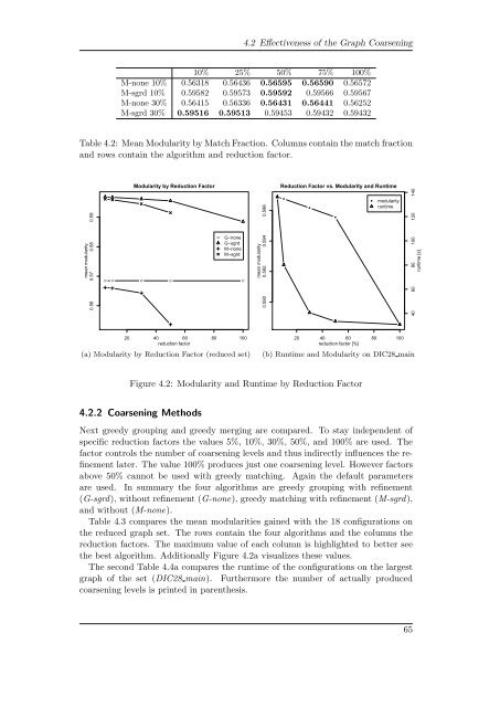
4.2 Effectiveness of the Graph Coarsening10% 25% 50% 75% 100%M-none 10% 0.56318 0.56436 0.56595 0.56590 0.56572M-sgrd 10% 0.59582 0.59573 0.59592 0.59566 0.59567M-none 30% 0.56415 0.56336 0.56431 0.56441 0.56252M-sgrd 30% 0.59516 0.59513 0.59453 0.59432 0.59432Table 4.2: Mean Modularity by Match Fraction. Columns contain the match fractionand rows contain the algorithm and reduction factor.mean modularity0.56 0.57 0.58 0.59Modularity by Reduction Factor● ● ● ● ●●G−noneG−sgrdM−noneM−sgrdmean modularity0.590 0.592 0.594 0.596●Reduction Factor vs. Modularity and Runtime●●●●modularityruntime40 60 80 100 120 140runtime [s]●20 40 60 80 100reduction factor(a) Modularity by Reduction Factor (reduced set)20 40 60 80 100reduction factor [%](b) Runtime and Modularity on DIC28 mainFigure 4.2: Modularity and Runtime by Reduction Factor4.2.2 Coarsening MethodsNext greedy grouping and greedy merging are compared. To stay independent ofspecific reduction factors the values 5%, 10%, 30%, 50%, and 100% are used. Thefactor controls the number of coarsening levels and thus indirectly influences the refinementlater. The value 100% produces just one coarsening level. However factorsabove 50% cannot be used with greedy matching. Again the default parametersare used. In summary the four algorithms are greedy grouping with refinement(G-sgrd), without refinement (G-none), greedy matching with refinement (M-sgrd),and without (M-none).Table 4.3 compares the mean modularities gained with the 18 configurations onthe reduced graph set. The rows contain the four algorithms and the columns thereduction factors. The maximum value of each column is highlighted to better seethe best algorithm. Additionally Figure 4.2a visualizes these values.The second Table 4.4a compares the runtime of the configurations on the largestgraph of the set (DIC28 main). Furthermore the number of actually producedcoarsening levels is printed in parenthesis.65