Meta-analysis of individual patient data versus aggregate data from ...

IPD versus aggregate data in the meta-analysis of longitudinal trials 17IntroductionThe assessment of a patient who has a chroniccondition, for example cystic fibrosis or a neurodegenerativedisorder, often involves taking measurementsof an outcome at a number of timepoints throughout the course of a trial. Such dataare referred to as longitudinal data or repeatedmeasures data, and allow one to assess the changein an outcome over a period of time [1]. Whenmultiple trials of the same longitudinal outcomeexist, it is clearly important to synthesize the dataacross trials to facilitate evidence-based conclusions.However, the longitudinal nature of thedata creates added complexity for those performingmeta-analysis. For example, it is common tofind that the timing of the repeated measurementsvaries across trials. In this situation,a standard meta-analysis conducted at a specifictime point will usually be based on only asubset of the trials. Further, meta-analyzing eachtime-point independently may be inappropriate,as correlation exists between time-points. Thus amore complex meta-analysis that synthesizes alltrials and all time-points simultaneously, whilstaccounting for correlation, is potentially superior.Several authors have considered the metaanalysisof longitudinal data [2–4]. Most recently,Ishak et al. consider when only aggregate dataare available from each study [4], such as themean treatment difference and its standard error ateach time-point. They propose models that accountfor the correlation between the multiple timepoints,and suggest the approach ‘may providebetter fit and possibly more precise summary effectestimates’ than approaches that ignore correlation.However, the authors note that they ‘encountereddifficulties in estimating the correlationparameters’, even when very simple correlationstructures were assumed, and could not confirm thebenefits of the proposed models since in theirexample ‘the true values of the parameters ofthe model were not known’. This highlightssome of the disadvantages of having onlyaggregate data, with the unavailability of withinstudycorrelations a major concern and limitation[5,6].In this article we consider the meta-analysis oflongitudinal data using individual patient data(IPD) [7], where the original data from allparticipants in each trial are obtained and thensynthesized. We show that availability of IPDallows the correlation between multiple timepointsto be calculated directly in each study,thus overcoming the aforementioned problemshown in Ishak et al. [4] when the correlationsare unknown. We describe how to appropriatelymeta-analyze IPD by: (i) using models that directlysynthesize the IPD in a one-step approach,or (ii) first reducing the IPD to aggregate data ineach study, and then synthesizing the aggregatedata across studies using a multivariate metaanalysismodel. This allows us to show therelationship between IPD and aggregate datamodels, and thus recommend how best to proceedwith aggregate data models when IPD are notavailable.The outline of the article is as follows. In section‘A review of current practice’ we summarizea review of practice for meta-analyzing longitudinalstudies in the Cochrane Library [8]. In section‘Methods for meta-analysis of longitudinal data’we describe methods for IPD and aggregate metaanalysisof longitudinal data, and in section‘Illustration of the meta-analysis methods’ theseare applied to an example where IPD are availablefor five Alzheimer trials, which enables us tocompare IPD and aggregate data approachesdirectly. Finally, in section ‘Discussion’ we criticallydiscuss our work and make recommendations forpractice and further research.A review of current practiceTo investigate current practice for meta-analyzinglongitudinal data we searched Issue 3 2005 ofthe Cochrane Library [8], which contained 2435completed reviews. We searched using the threeterms ‘longitudinal*’, ‘repeated NEXT measure*’and ‘serial NEXT measure*’, and reviews neededto contain one or all of these search terms tobe identified. The term ‘longitudinal*’ was foundin 289 reviews (12%), the term ‘repeated NEXTmeasure*’ in 70 (3%) and ‘serial NEXT measure*’in 6 (0.25%). These results related to 345 independentreviews, but after further investigationonly 113 reviews related to a longitudinal datameta-analysis.In 85 of these 113 reviews the Methods sectioncontained no information regarding the analysisof longitudinal data; however in 22 of thesethe Results section indicated that a separatemeta-analysis had been carried out at each of anumber of time points, with the correlationbetween time points not taken into account.Indeed, the issue of correlated data was notdiscussed in the Results or Discussion sectionof any of these reviews. The remaining 28 reviewsdid discuss the analysis of longitudinal data inthe Methods section, as follows: (i) in 15 reviewsit was stated that an analysis at separate time pointswould be conducted, although this was ultimatelyonly possible in 10 due to the lack of data; (ii) inhttp://ctj.sagepub.com Clinical Trials 2009; 6: 16–27Downloaded from http://ctj.sagepub.com at University of British Columbia Library on June 15, 2009

18 AP Jones et al.six reviews authors stated that they would choosedata from one of the time points from each of thetrials (four of these reviews pre-specified that theywould analyze data from the final time pointreported in the trials and two stated that theywould analyze the data reported at the time pointnearest to the one pre-specified in their protocol);(iii) in five reviews it was mentioned that the lengthof follow up was a possible source of heterogeneityacross trials (two of these studies ultimatelyused single time point analysis and three did nothave any data to perform a meta-analysis); (iv) inone review the authors stated that the statisticalpackage used within Cochrane reviews was notappropriate for analyzing longitudinal data andso they just reported the results from the originaltrials in a table; and (v) in the remaining reviewincidence rates based on person time were reported.It is thus clear from this review that practitionersare undecided on how to appropriately metaanalyzelongitudinal studies, and it seems thatonly simple meta-analysis methods are used.In particular, ignoring correlation between timepoints and undertaking a meta-analysis at eachof the several time points separately was the mostfrequently used method in practice.Since this review of the literature was conducted,there has been limited research into the analysisof data of this form [4] and we therefore feel thatthe situation has not changed a great deal andreview authors are still not analyzing this formof data using the most appropriate methods. Ourarticle gives a number of methods that could beused depending on the information that is availableto the review author.Methods for meta-analysis oflongitudinal dataIn this section, appropriate methods for an IPDanalysis of longitudinal continuous outcome dataare described, first for a single study and then fora meta-analysis of several studies. Models arepresented both for time as a factor and asa continuous variable, and they assume fixedtreatment effects across studies. We then consideraggregate data meta-analysis of longitudinal data,and describe the aggregate data required to producesimilar results to the IPD meta-analysis. Extensionto random treatment effects is considered in thediscussion.Across the studies in the meta-analysis, observationsmay have been recorded at differenttime points post-treatment. Our notation belowregarding time points assumes that all of thetime points which have occurred in any of thestudies have been ordered and are referred to ast k (k ¼ 1, ..., b). Thus any one trial may only provideobservations for some of the b time points. Also, fora particular study an assessment may have beenperformed prior to any study treatment (baseline).Our models below assume that there areonly post-treatment assessments. However, modificationsto the models to include baseline measurementsin the response variable as an additionalassessment time will be discussed briefly whererelevant.IPD from a single studyTreating time as a factor, a model for a single study(study i) which includes treatment, time andtreatment by time interaction terms is given byy hijk ¼ ik þ hik þ " hijk ;ð1Þwhere y hijk is the observation in study i from patientj (j ¼ 1, ..., n hi ) on treatment h (h ¼ 1, ..., a) attime t k , and " hijk is the residual error. In thisarticle we take treatment a to be the referencetreatment, so that hik represents the effect oftreatment h minus the effect of treatment a attime t k , and aik ¼ 0. The parameter ik is the effectof treatment a at time t k . If required, baselineobservations can be included as observations y hij0and model (1) defined for k ¼ 0, 1, ..., b. Usuallyin randomized controlled trials the parameters hi0 ,h ¼ 1, ..., a, would be set equal to zero as nodifferences due to treatment are expected atbaseline.Alternatively, treating time as a continuousvariable with a linear effect the model can bewritten asy hijk ¼ i þ hi þ i t k þ hi t k þ " hijk ;ð2Þwhere i is the intercept for treatment a, hi isthe difference in the intercepts between treatmenth and treatment a ( ai ¼ 0), i is the time slope fortreatment a, and hi is the difference in the timeslopes between treatment h and treatment a( ai ¼ 0).Model (2) incorporates separate intercepts foreach treatment, thus only making the assumptionof a linear trend with time over the time pointsincluded in the model. If the baseline observationsare to be included or a linear trend from time ¼ 0is to be fitted, then hi would be removed from themodel.In both models (1) and (2), the " hijk are assumedto be normally distributed with zero meanand a covariance structure that allows for thecorrelation between repeated observations on theClinical Trials 2009; 6: 16–27http://ctj.sagepub.comDownloaded from http://ctj.sagepub.com at University of British Columbia Library on June 15, 2009

IPD versus aggregate data in the meta-analysis of longitudinal trials 19same patient. There are various possible structuresone could use [9]: for example, a fully unstructuredcovariance matrix would allow a separate varianceparameter for each time point within eachtreatment group, and a separate covarianceparameter for each pair of time points (k and m,say) in each treatment group, so thatandV " hijk¼ 2hikð3ÞCov " hijk , " hijm¼ hikm hik him for k 6¼ m, ð4Þwhere hikm is the correlation between observationsfrom the same patient in treatment group h at timepoints k and m. Simpler specifications are alsopossible; for instance, we could assume commonvariances and correlation coefficients across alltimes and treatment groups. However, in thisarticle we use the fully unstructured covariancematrix above in all of our analyses. The majoradvantage of this is that it allows the correlationbetween time points close together to be largerthan the correlation between time points which arefarther apart. The disadvantage is that it requires alarge number of parameters to be estimated [10].In some situations, the autoregressive covariancestructure might be used as an acceptable compromise.Equations (1) and (2), and all subsequentmodels in this article, can be fitted using softwarefor repeated measurements analysis, for exampleSAS PROC MIXED [11] (model codes are availableon request).IPD meta-analysis of several studiesWhen IPD are available from each of the studies,the meta-analysis can proceed in a one-step ora two-step framework [7]. The one-step approachsimultaneously models the IPD from all of thestudies. The two-step approach first fits a model tothe IPD from each study separately, and thenthe study parameter estimates are combined in ameta-analysis. We discuss both approaches in thissection: it is the second approach which linksdirectly with an aggregate data approach when IPDare unavailable.One-step IPD meta-analysis of several studiesAssume that IPD are available from r independentstudies (i ¼ 1, ..., r) and let us extend Equation (1)assuming that the true underlying treatment effectat each time-point is fixed across studies. In thissituation the interaction terms study by treatmentand study by treatment by time can be excludedfrom the model. For time as a factor, the model canbe writteny hijk ¼ ik þ hk þ " hijk ;ð5Þwhere ik is the effect of treatment a at timet k in study i, and hk represents the effectof treatment h minus the effect of treatment a attime t k , which is common across all studies( ak ¼ 0). If required, baseline assessments can beincluded as observations y hij0 , and model (5)defined for k ¼ 0, 1, ..., b. Usually the parameters h0 , h ¼ 1, ..., a, would be set equal to zero asno differences due to treatment are expected atbaseline.For time as a continuous covariate, Equation (2)can be extended to becomey hijk ¼ i þ h þ i t k þ h t k þ " hijkð6Þwhere i is the intercept for treatment a in studyi thus allowing for different prognostic groupsentered across the trials, h is the intercept fortreatment h minus the intercept for treatment a,which is common to all studies ( a ¼ 0).The parameter i is the time slope for treatmenta in study i, and h is the difference in the timeslopes between treatment h and treatment a, whichis common to all studies ( a ¼ 0). If the baselineobservations are to be included or a linear trendfrom time ¼ 0 is to be fitted, then h would beremoved from the model.In Equations (5) and (6), using the fullyunstructured covariance matrix each study has aseparate variance parameter for each time pointwithin each treatment group, and a separatecovariance parameter for each pair of time pointswithin each treatment group (as in Equations (3)and (4)). Overall estimates of the mean treatmentdifference at each time point can be obtained: thesewould be ^ hk if using Model (5), and ^ h þ ^ h t kif using Model (6). T-tests and confidence intervalsbased on the t-distribution can be calculated.SAS PROC MIXED allows the option to inflatethe estimated variance of the mean treatmentdifference to allow for the estimation ofthe variance and covariance components and toestimate the degrees of freedom for the t-test usingSatterthwaite’s procedure [12,13].Two-step IPD meta-analysis of several studiesIn the first step of the two-step IPD meta-analysisapproach, each study is analyzed separately. Whentime is to be treated as a factor, Model (1) is fitted tohttp://ctj.sagepub.com Clinical Trials 2009; 6: 16–27Downloaded from http://ctj.sagepub.com at University of British Columbia Library on June 15, 2009

20 AP Jones et al.each study to produce estimates, variances, andcovariances of the mean difference between treatmenth and treatment a (h ¼ 1, ..., a 1) at eachrecorded time point. Let d hik (h ¼ 1, ..., a 1) be theestimate of the mean difference between treatmentsh and a at time t k in study i, that is d hik ¼ ^ hik .When time is to be treated as a continuous variable,Model (2) is fitted to each study to produceestimates, variances and covariances of the differencesin the intercepts and time slopes betweentreatment h and treatment a (h ¼ 1, ..., a 1). Let f hi(h ¼ 1, . . . , a 1) be the estimate of the difference inintercepts, that is f hi ¼ ^ hi , and g hi (h ¼ 1, ..., a 1) bethe estimate of the difference in time slopes, that isg hi ¼ ^ hi .The second step requires a multivariate metaanalysisframework [14], which allows the jointsynthesis of the d hik (or f hi and g hi ) values acrossstudies. The weighting for each d hik (or f hi and g hi ) isa function of its variance and covariance with otherestimates from the same study. For time as a factor,the model is given byd hik ¼ hk þ hik ;ð7Þwhere hik is the residual error, and the hik from thesame study are correlated.When time is a continuous variable, there aretwo model options. The first uses the studyestimates of the differences in intercepts and thedifferences in slopes as the responses and fits themodel given byf hi ¼ h þ hig hi ¼ h þ hið8aÞwhere hi and hi are residual errors, which arecorrelated within a study. A second option usesthe estimates of the mean difference betweentreatments h and a at time t k in each study as theresponses and fits the model given byd hik ¼ h þ h t k þ hikð8bÞwhere hik is the residual error, and the hik from thesame study are correlated. In both cases, the effectof treatment h minus the effect of treatment a attime t k is given by h þ h t k .In common practice in the meta-analysis field,the variance and covariance terms for the d hik (or f hiand g hi ) calculated in the first step are used inthe second step as the variance and covariance ofthe residual errors, and treated as if they were thetrue variances and covariances. The multivariatemeta-analysis in the second step may befitted using SAS PROC MIXED [11], as describedelsewhere [15], in which the d hik (or f hi and g hi )values are the observations in the dataset. Whenusing the f hi and g hi values a study must have datafor at least two time points to be included in theanalysis: if there is only one time point f hi and g hicannot be calculated.Overall estimates of the mean treatmentdifference at each time point can be obtained:these would be ^ hk if using Model (7), and ^ h þ ^ h t kif using Models (8a) or (8b). Assuming thatthe variances are known, hypothesis tests andconfidence intervals may be based on the normaldistribution.One-step versus two-step approachAlthough the two IPD approaches should providesimilar results, they will not be identical for severalreasons. First, the two-step approach allows for thepossibility of study by treatment and study bytreatment by time interactions when calculatingthe variance and covariance terms of the d hik(or f hi and g hi ), although the actual model fitted tothe d hik (or f hi and g hi ) does not. The one-stepmethod based on Models (5) or (6) does not includethese interaction terms at all. The effect that thishas on the results depends on the magnitude ofthese interaction terms.A second factor which may produce a differencebetween the two IPD approaches is the amountof missing data at the patient-level within a study[16]. Under a missing at random assumption,Equations (1), (2), (5), and (6) can accommodatepatients, who do not supply data at each time pointin the study. Indeed, under this assumption thecorrelation between time points is used to improvethe estimation of the parameters and this results in‘model-based’ estimates (section ‘Meta-analysisof aggregate data’). As parameter estimates andvariances are dependent on the model terms as wellas the structure of the covariance matrix, this maylead to differences in the estimates between the twoIPD approaches. This factor is also important whenwe consider the aggregate data methods in section‘Meta-analysis of aggregate data’.Meta-analysis of aggregate dataAn aggregate data meta-analysis of longitudinaldata clearly depends on the aggregate data availablefrom trials [17]. If the estimates d hik (or f hi and g hi )and their variances and covariances are available,then the second part of the two-step IPD analysesdescribed in section ‘Two-step IPD meta-analysis ofseveral studies’ can be undertaken directly.However, often trials only report means andstandard deviations for each treatment groupat each time point. In this section we thus describeClinical Trials 2009; 6: 16–27http://ctj.sagepub.comDownloaded from http://ctj.sagepub.com at University of British Columbia Library on June 15, 2009

IPD versus aggregate data in the meta-analysis of longitudinal trials 21methods which are based only on these summarystatistics, and discuss the implications that this hasfor the validity of the meta-analysis.Let y hi:k be the mean of the n hik observationsfrom treatment h at time t k in study i, and z hik ¼y hi:k y ai:k . Then z hik is an estimate of the effect oftreatment h minus the effect of treatment a at timet k , and the model for the z hik based on Model (1) isgiven by" ai:kz hik ¼ hik þ ð" hi:k Þ ð9ÞWe refer to z hik as a raw estimate of the meantreatment difference as it is based on raw means(this is in contrast to the model-based estimates oftreatment difference discussed in section ‘One-stepversus two-step approach’, which may be subtlydifferent). Assuming that the treatment groupscontain independent sets of patients, the varianceof z hik is given byhave the covariance structure given by Equations(10) and (11). However, in the case when there aremissing data at the patient-level, d hik and z hikmay be subtly different; the d hik are model-basedestimates, which adjust for the missing patient dataacross time points, unlike the z hik , and so the d hikand their covariance structure will be a modificationof Equations (10) and (11) [14]. Consequently,if there are any missing patient-level data thetwo-step IPD approach will use model-based estimates,of treatment difference, and their variancesand covariances, whilst the aggregate dataapproach will only use raw estimates, and theirvariances and covariances. The magnitude of thedifferences between the model-based and raw meantreatment differences will depend on the patternand amount of missing data. Large differences maysubsequently cause a discrepancy in the resultsfrom the two-step IPD meta-analysis and theaggregate data meta-analysis of raw means.Vz hikð Þ ¼ Vð" hi:k " ai:k Þ ¼ 2 hikþ 2 aikn hikn aikð10ÞAlso, for k 6¼ m, the covariance between theobserved mean difference at time point k andthe observed mean difference at time point m isgiven byCovðz hik , z himÞ ¼ Covð" hi:k , " hi:m¼ q hikm hihm hik himn hik n himþ q aikm aihm aik aimn aik n aimÞ þ Covð" ai:k , " ai:m Þð11Þwhere q hikm is the number of patients contributingto both time points k and m in treatment group h.Meta-analysis of aggregate data – time as a factorTo perform a meta-analysis of the aggregate datawhich is close to the two-step IPD meta-analysisdescribed in section ‘Two-step IPD meta-analysis ofseveral studies’, the z hik values and estimatesof their variances and covariances based onEquations (10) and (11) need to be calculatedfor each study. These are used in the second stepof the two-step IPD meta-analysis, so that model (7)is replaced by" ai:kz hik ¼ hk þ ð" hi:k Þ: ð12ÞIf all patients provide data at all time pointsin trial i, the d hik values from the IPD analysis oftrial i, based on the fully unstructured covariancematrix, are equal to the raw z hik values and theyMeta-analysis of aggregate data – time as a continuousvariableTo perform a meta-analysis of the aggregate datawith time treated as a continuous variable, the z hikvalues and estimates of their variances and covariancesbased on Equations (10) and (11) could beused in the second step of the two-step IPD metaanalysis,with model (8b) replaced by" ai:kz hik ¼ h þ h t k þ ð" hi:k Þ: ð13ÞThe effect of treatment h minus the effectof treatment a at time t k is given by h þ h t k .Estimates of the mean treatment differencesfrom the aggregate data approach may be similar,but not identical to those from the two-stepIPD approach. When time is considered as acontinuous variable, deviations from the fittedstraight line with time are not incorporated inthe variance and covariance terms for theaggregate data approach, whereas they are inthe first step of the two-step IPD approach.Further, as discussed in section ‘Meta-analysis ofaggregate data – time as a factor’, when thereare missing patient data the model-based estimatesfrom the IPD may differ subtly from the raw z hikestimates.Unavailable aggregate dataA major issue for the meta-analysis of raw meansis that the covariance defined by Equation (11)cannot often be calculated, as hik , q hikm , and hikmhttp://ctj.sagepub.com Clinical Trials 2009; 6: 16–27Downloaded from http://ctj.sagepub.com at University of British Columbia Library on June 15, 2009

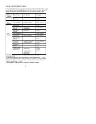
22 AP Jones et al.will rarely be available from publications, andso approximations are necessary. If s hik denotesthe standard deviation for treatment grouph at time point k in study i, then this can be usedas an estimate of hik . The q hikm values mightbe approximated by the minimum of n hik andn him . The hikm values could be approximated byone of two approaches. One could take a simplisticapproach and assume one common correlationacross all studies, treatments and time points.More appropriately, one could perform a sensitivityanalysis to ascertain if and how the meta-analysisresults change with the value of the correlationcoefficient imputed [14]. In some situations itmay also be more appropriate to assume differentimputed correlations for each pair of time points,though this approach will become increasinglycomplicated as the number of time pointsincreases. Note that setting the hikm equal tozero leads to a standard meta-analysis conductedat each time point separately. This is the commonmethod in practice (section ‘A review of currentpractice’), but it is a strong assumption to makeas longitudinal data are often highly correlated [1].It leads to an estimate of the mean differencebetween treatment h and treatment a at time pointk given byX rw hik z hik1with variance Pw rhiki¼1 w ,hik1:where w hij ¼ s 2 hik =n hik þ s 2 aik =n aiki¼1Hypothesis tests and confidence intervals maybe based on the normal distribution [18].Illustration of the meta-analysismethodsTo illustrate and compare the IPD and aggregatedata meta-analysis methods, we now considera systematic review of trials investigatingthe effects of selegiline versus placebo for thetreatment of Alzheimer’s disease [19]. Five trialsprovided IPD for the mini-mental state examination(MMSE), a measure of cognitive function,and in this article we focus on just these fivestudies as they allow us to empirically compareIPD and aggregate data approaches. In eachof the trials the dosing schedule was thesame (10 mg/day) and they all had a differentlength of treatment with no common time point.The MMSE can take values from between 0 and30, with higher values being regarded as good,and is considered in our analyses to be approximatelynormally distributed.To illustrate the methods presented in thisarticle, the results have been grouped to createcommon time points. That is: month 1 ¼ weeks4 and 5; month 2 ¼ weeks 8 and 9; month 4 ¼ week17; month 6 ¼ weeks 24, 25, and 30; month9 ¼ week 35 and 43; month 12 ¼ weeks 56 and 65.Some patients withdrew before the completionof all of the assessments and no single studygave results for each time-point; thus thereare missing data in at the patient-level andalso at the study-level. Table 1 taken fromTable 9.6 of Whitehead [18] shows the rawmeans and standard deviations for eachtreatment at each time point in each study.From these values the raw mean differences andTable 1Raw summary statistics for MMSE dataMonthStudyPlaceboSelegilineTreatment effect(Selegiline – placebo)Number ofsubjectsMeanStandarddeviationNumber ofsubjectsMeanStandarddeviationMean, z hik Variance, V(z hik )1 3 24 17.08 4.33 22 17.73 6.78 0.65 64.724 166 12.33 5.61 165 13.07 5.40 0.74 60.635 25 19.88 6.27 25 17.72 5.67 2.16 71.462 1 20 18.30 4.40 18 18.78 6.28 0.48 58.803 23 18.04 5.00 23 17.43 6.71 0.61 70.025 24 19.33 6.35 25 17.56 4.93 1.77 64.634 3 20 17.20 4.49 23 18.00 6.28 0.80 59.604 151 11.84 5.57 156 12.28 5.47 0.44 60.956 2 68 20.32 5.16 64 19.80 5.46 0.52 56.443 18 16.33 5.40 23 17.74 6.24 1.41 68.104 139 11.14 5.95 144 11.23 5.68 0.09 67.669 1 18 16.17 6.22 17 17.12 6.38 0.95 79.394 125 9.94 6.01 134 10.45 5.74 0.51 69.0712 1 17 15.47 6.34 15 13.07 7.41 2.40 95.104 112 9.59 6.01 121 9.79 6.05 0.20 72.72Clinical Trials 2009; 6: 16–27http://ctj.sagepub.comDownloaded from http://ctj.sagepub.com at University of British Columbia Library on June 15, 2009

IPD versus aggregate data in the meta-analysis of longitudinal trials 23their variances (i.e., the z hik and V(z hik ) values) canbe calculated.The meta-analysis models described in section‘Methods for meta-analysis of longitudinal data’were applied to the MMSE data to compareresults from the one-step IPD analysis withthe two-step IPD analysis of model-basedestimates, and also the aggregate data metaanalysisof raw estimates. For illustrative purposesboth time as a factor and time as a continuousvariable were considered. However, it should benoted that the continuous model is perhaps notentirely appropriate for this data set. Figure 1shows a plot of the differences between selegilineand placebo across time.Time as a factorIPD meta-analyses: one-step versus two-step usingcorrect covariancesThere are no statistically significant differencesbetween the two treatments at any of the timepoints when time is treated as a factor (Table 2).As discussed in section ‘One-step versus two-stepapproach’ the results from the one-step (Equation(5)) and the two-step IPD meta-analysis (model (1)in each study followed by model (7) using thecorrect covariance estimates) can differ, but for thisexample the results are very similar.IPD meta-analyses: one-step versus two-step imputingcovariancesAs part of our analyses, we considered how thetwo-step meta-analysis results would change if theMean difference in MMSE−2 −1 0 1 20 20 40 60WeekStudy1Study3Study5Study2Study4Figure 1 Plot of raw mean differences in MMSE (selegeline –placebo) against timeTable 2 Meta-analysis of MMSE data treating time as a factor: estimates (standard error) of difference between Selegiline and PlaceboAggregate data Equation (12), covarianceestimates from Equation (11) with hik ¼ s hikTwo-step IPD Equation (1) in each study,followed by Equation (7)Time point One-step IPDEquation (5) hikm ¼ 0.8 hikm ¼ 0.4 hikm ¼ 0Correlations of0 between dhikCorrelations of0.4 between dhikCorrelations of0.8 between dhikCorrect covarianceestimates for dhik1 month 0.31 (0.47) 0.30 (0.47) 0.30 (0.48) 0.34 (0.52) 0.43 (0.54) 0.40 (0.48) 0.39 (0.53) 0.44 (0.54)2 months 0.48 (0.62) 0.47 (0.59) 0.37 (0.65) 0.58 (0.88) 0.84 (0.97) 0.22 (0.69) 0.42 (0.91) 0.70 (0.99)4 months 0.34 (0.48) 0.33 (0.47) 0.39 (0.49) 0.52 (0.55) 0.75 (0.57) 0.19 (0.51) 0.29 (0.57) 0.49 (0.59)6 months 0.20 (0.49) 0.19 (0.48) 0.22 (0.48) 0.23 (0.50) 0.31 (0.50) 0.10 (0.51) 0.08 (0.52) 0.00 (0.53)9 months 0.35 (0.53) 0.34 (0.52) 0.33 (0.53) 0.47 (0.60) 0.69 (0.63) 0.31 (0.60) 0.39 (0.67) 0.56 (0.69)12 months 0.02 (0.56) 0.03 (0.55) 0.10 (0.56) 0.05 (0.63) 0.29 (0.66) 0.30 (0.66) 0.21 (0.73) 0.04 (0.75)http://ctj.sagepub.com Clinical Trials 2009; 6: 16–27Downloaded from http://ctj.sagepub.com at University of British Columbia Library on June 15, 2009

24 AP Jones et al.model-based mean differences and their varianceswere available from each study, but without theircovariances, as this situation may occur in practice.We thus fitted Equation (7) to the model-basedestimates for each of correlations 0.8, 0.4, and0 (Table 2). It can be seen that the pooled treatmentdifference estimates when the correlation is 0.8are similar to those using the correct covarianceestimates. This is not surprising as the actualcorrelations between time point estimateswere of a similar magnitude. As the correlationcoefficient becomes smaller, the treatmentdifference estimates move further away fromthose based on the correct covariance estimates.Indeed the assumption of zero correlation, asis usual in practice, produces estimates, andstandard errors that are very different from thosebased on the correct covariance estimates. Forexample, assuming zero correlation gives a pooledtreatment difference at 9 months of 0.69,with standard error of 0.63, compared to the trueanswer of 0.34, with standard error of 0.52.Importantly, though, the standard errors areconservative in this situation, a finding consistentwith analytical assessment of longitudinal data ina non meta-analysis setting when time is taken as afactor [20].Aggregate data meta-analysesWe now assume that trials only provide their rawmeans and standard deviations, and not their IPD.As discussed in section ‘Unavailable aggregate data’,to perform the aggregate data meta-analysis in thissituation we needed to approximate hik and q hikm ,and we then fitted meta-analysis model (12)for each of hikm equal to 0, 0.4, and 0.8 (Table 2).There is a considerable amount of missing patientdata in the MMSE studies and thus the rawestimates of treatment difference differ considerablyfrom the model-based estimates derived fromIPD, as discussed in section ‘Meta-analysisof aggregate data – time as a factor’. This leadsto differences between the aggregate data metaanalysisresults and those from the one-stepand two-step IPD analyses (Table 2). For example,in the analyses assuming a correlation of 0.8, at12 months the aggregate data meta-analysis givesa pooled treatment difference of 0.30, withstandard error of 0.66, compared to the trueanswer of 0.03, with standard error of 0.55.However, importantly the standard error of theaggregate data meta-analysis results is again alwaysconservative and, in this particular example, theconclusions from the aggregate data meta-analysisare the same as those from the IPD analyses,Table 3 Meta-analysis of MMSE data treating time as a continuous variable: estimates (standard error) of difference between Selegiline and Placebo (Study 2 excluded*)Aggregate data Equation (13),covariance estimates fromEquation (11) with hik ¼ s hikTwo-step IPD Equation (1) in eachstudy, followed byEquation (8b)Two-step IPD Equation (2)in each study, followed byEquation (8a)One step IPDEquation (6) hikm ¼ 0.8 hikm ¼ 0.4 hikm ¼ 0correlations of0 betweencorrelations of0.4 betweencorrelations of0.8 betweencorrect covarianceestimates forCorrect covarianceestimates forfhi and ghidhikdhikdhikdhikIntercept estimate 0.38 (0.53) 0.37 (0.52) 0.45 (0.51) 0.52 (0.49) 0.43 (0.48) 0.38 (0.46) 0.47 (0.51) 0.41 (0.49) 0.36 (0.47)Slope estimate 0.005 (0.036) 0.005 (0.036) 0.015 (0.035) 0.020 (0.033) 0.007 (0.055) 0.017 (0.067) 0.018 (0.047) 0.005 (0.063) 0.019 (0.073)Time point1 month 0.37 (0.52) 0.37 (0.51) 0.43 (0.50) 0.50 (0.49) 0.42 (0.45) 0.40 (0.40) 0.45 (0.50) 0.40 (0.46) 0.38 (0.41)2 months 0.37 (0.52) 0.36 (0.51) 0.42 (0.50) 0.48 (0.49) 0.41 (0.43) 0.41 (0.35) 0.43 (0.49) 0.40 (0.43) 0.40 (0.36)4 months 0.36 (0.52) 0.35 (0.51) 0.39 (0.50) 0.44 (0.49) 0.40 (0.40) 0.45 (0.28) 0.40 (0.50) 0.39 (0.41) 0.44 (0.29)6 months 0.35 (0.53) 0.34 (0.52) 0.36 (0.51) 0.40 (0.50) 0.39 (0.40) 0.48 (0.26) 0.36 (0.52) 0.38 (0.42) 0.48 (0.28)9 months 0.33 (0.56) 0.32 (0.55) 0.31 (0.54) 0.34 (0.53) 0.37 (0.45) 0.53 (0.34) 0.31 (0.58) 0.36 (0.50) 0.53 (0.38)12 months 0.32 (0.61) 0.31 (0.60) 0.26 (0.59) 0.28 (0.57) 0.35 (0.55) 0.58 (0.50) 0.25 (0.67) 0.35 (0.63) 0.59 (0.56)*Study 2 had to be excluded from the analysis using Equation (8a) as it had only one time point result and thus did not provide an intercept and slope estimate. Study 2 could havebeen included in the other analyzes presented, but to ensure comparability it was also removed from these.Clinical Trials 2009; 6: 16–27http://ctj.sagepub.comDownloaded from http://ctj.sagepub.com at University of British Columbia Library on June 15, 2009

IPD versus aggregate data in the meta-analysis of longitudinal trials 25namely that there is no evidence that selegilineis beneficial.Time as a continuous variableOne-step IPD analysis versus two-step IPD analysis ofintercept and slopeThe results from the IPD meta- analyses when timeis treated as a continuous variable and a linearregression is fitted are shown in Table 3. As a linearregression model could not be fitted to study 2,because it only provides data at one post-treatmenttime point, the two-step meta-analysis of intercepts,and slopes had to exclude this study. Forcomparability study 2 has also been excluded fromall meta-analyses treating time as a continuousvariable.The one-step IPD meta-analysis gives resultsthat are almost identical to the two-step analysisof model-based intercept and slope estimates (usingthe correct covariances). There is no evidence thatthe difference between selegiline and placebofollows a linear trend over time or that selegilineis better than placebo.four and seven in ‘9 months’ row in Table 3). Thisis important, as practitioners may place anoverconfidence in their results in this situation.Furthermore, assuming zero correlation changesthe slope of the fitted regression line from negative( 0.015) to positive (0.017), although there isstill no evidence of a linear trend over time orthat selegiline is beneficial.The two-step meta-analysis using the raw treatmentdifference produces results that differ slightlyto those from the meta-analysis of model-basedestimates. The key observation again, though,is that assuming zero correlation seriously underestimatesthe standard error of pooled estimates.For example, at six months the true result (i.e., thatfrom using the model-based estimates with correctcovariances) is a pooled treatment difference of0.36, with standard error of 0.51, but the analysisof raw means assuming zero correlation givesa pooled estimate of 0.48, with standard error0.28. Thus, for time as continuous, it is clear thattreating the correlation as zero does not lead toconservative standard errors, a finding consistentwith analytical assessment of longitudinal data ina non meta-analysis setting when time is taken ascontinuous [20].Two-step analysis of model-based or raw time pointestimatesThe two step method in section ‘One-step IPDanalysis versus two-step IPD analysis of interceptand slope’ assumes that the slope and interceptterms are available from each study. Theseestimates are very rarely reported by trial authorsand so, if the IPD are not available, the only optionmay be to fit a regression line to either themodel-based or raw estimates of treatment differenceat each time point (see Equations (8b) and(13), respectively). We thus fitted a regression lineto both the model-based and raw time pointestimates for the MMSE data (Table 3).The two-step analysis using the model-basedtime point and correct covariance estimates givesa negative slope estimate of 0.015, slightly largerthan the negative slope estimate of 0.005 fromthan the two-step analysis based on model-basedintercept, slope, and correct covariance estimates.If we also assume that the covariance estimates areunavailable, as likely in practice, the assumption ofzero correlation between the model-based timepoint estimates causes the standard error of thepooled estimates of treatment difference to be toosmall (Table 3). For example, assuming zerocorrelation gives the standard error of the pooledtreatment difference at 9 months to be 0.34,whereas the true answer is 0.54 (compare columnsDiscussionWhen conducting a meta-analysis of longitudinaldata, it is preferable to obtain the IPD from allof the studies that were identified from thesystematic review. This facilitates meta-analysismodels that correctly account for the correlationbetween repeated observations for the same patientin each trial. In this article we have presentedsuch IPD meta-analysis models, which use either aone-step or a two-step approach. Application to theAlzheimer’s data set confirms that these approachesare preferable to an analysis that assumesno correlation between repeated observations, fora number of reasons. First, the pooled estimateswhen assuming zero correlation can differ considerablyfrom the correct answers, although in ourparticular example clinical conclusions wereunaffected. Second, when time is treated as afactor, the analyses including correlation weremore efficient, with the standard error of pooledestimates much smaller than in analyses assumingzero correlation. Third, when time is treated ascontinuous, the analyses assuming zero correlationseverely underestimate the standard error of estimates,which in practice may lead to wrongconclusions. These findings are consistent withthose regarding ignoring correlation in the analysisof single studies [20], and are especially importanthttp://ctj.sagepub.com Clinical Trials 2009; 6: 16–27Downloaded from http://ctj.sagepub.com at University of British Columbia Library on June 15, 2009

26 AP Jones et al.given that our review of current practice (section ‘Areview of current practice’) identified that the mostcommon method for meta-analyzing longitudinaldata is to synthesize each time-point independently.We thus strongly recommend that, whereverpossible, practitioners should obtain IPD andthen perform a meta-analysis that accordinglyaccounts for correlation.We are aware, though, that it may not always bepossible to obtain IPD from trialists, and so we havealso presented possible methods for an aggregatedata meta-analysis in this situation. The idealaggregate data to obtain are the model-basedstudy estimates, and their variance and covarianceestimates, as these allow the IPD meta-analysisresults to be closely replicated (Tables 2 and 3) evenwhen there is a considerable amount of missingpatient data. Model-based estimates may be availablebut without their relevant covariances (e.g.,the covariance of treatment difference estimatesbetween time points), so we have shown how toperform sensitivity analyses to investigate therobustness of meta-analysis conclusions to differentvalues of imputed correlation. In doing so, we haveassumed that the imputed correlation is the samefor each pair of time points, which is simplistic.One could impute different correlations for eachtime-point, but this greatly increases the number ofparameters to be imputed. As an aid, data fromexternal studies in the same or similar indicationscould be used to inform the choice of values for thecorrelations and the extent of the variation acrossdifferent pairs of time-points.Though an aggregate data meta-analysis ofmodel-based estimates is the ideal aggregatedata approach, the model-based estimates maythemselves be unavailable, and indeed often onlytreatment means and standard deviations at eachtime point are available in our experience.We have shown how these can be used to calculateraw mean differences and their variances, whichcan be considered as an approximation to themodel-based estimates and their variances. Thenessentially the same modeling framework can beused as we described for model-based estimates andtheir variances. Again, a range of correlationcoefficients should be investigated in a sensitivityanalysis. It is inadvisable to ignore the correlationbetween repeated observations and it should not betreated as zero without good reason. In ourexamples the assumption of zero correlation didnot change the clinical conclusions and that initself is an important finding, but it is notinconceivable that in other situations clinicalconclusions may differ depending on thecorrelation.Regardless of whether IPD are available, reviewauthors need to consider carefully whether to fittime as a factor or a continuous variable within thelongitudinal models. We have considered bothapproaches in this model. However, the modelspresented for time as a continuous variable assumea linear effect of time. If this is an inappropriateassumption, then treating time as a factor willbe preferable. Alternatively, other models could beconsidered, but as they become more complicatedthis will necessitate IPD.When a meta-analysis of longitudinal datais carried out, it would be preferable if all thestudies were of the same duration and each studymeasured and reported results at the same timepoints. In reality this is unlikely to happen, and soto use the models presented in this article the timepoints need to be grouped together, preferablybased on clinical judgment and prespecified in thereview protocol. If analyses are done post-hoc, thenthis should be reported as such with sensitivityanalyses to the choice of groupings. Furthermore,when assessing multiple longitudinal data studies,it is perhaps inevitable that missing data will bean issue. The models presented assume thatany missing data is missing at random, both atthe patient-level and the study-level. It isclearly important for practitioners to clarify thetype and amount of missing data in their studies,and consider the potential impact of missingdata on their conclusions. For example, theyshould be aware that trials may only presenttime points showing a significant treatmentdifference, a problem known as within-studyselective reporting [21].All the models in this article assume fixedtreatment effects across studies, and we foundno evidence of between-study heterogeneity intreatment effect across the five trials in theAlzheimer’s example. This assumption may notalways be appropriate, but there are a number ofimportant issues to consider before extension torandom treatment effects. For example, shouldthere be a between-study heterogeneity parameterat each time-point, and should there be a separatebetween-study correlation between each pairof time-points? Estimation of the between-studycorrelation may also be difficult in some situations[22]. Ishak et al. propose aggregate data modelsfor meta-analysis of longitudinal data includingrandom-effects, but note that correlationparameters were difficult to estimate [4]. Thismay in part be due to unavailable within-studycorrelations in their example. Future work shouldthus extend our IPD and aggregate data methodsto include a random treatment effect across studies[23], and indeed develop meta-regression modelsto assess the impact of study-level covariates [24].A Bayesian approach to our models is alsopossible [25] and would allow prior informationClinical Trials 2009; 6: 16–27http://ctj.sagepub.comDownloaded from http://ctj.sagepub.com at University of British Columbia Library on June 15, 2009

IPD versus aggregate data in the meta-analysis of longitudinal trials 27about the correlation coefficients to be included[26]. A further issue, which has not been consideredin this article is how to perform a meta-analysiswhen some studies provide IPD and others onlyprovide aggregate data [27]. Goldstein et al suggestusing a multi-level approach to this problem [28],and this approach has recently been extendedto multiple outcomes [29].AcknowledgmentsWe thank the trialists of the selegiline studies whokindly provided the MMSE individual patient data.Whilst undertaking this work Richard Riley wasfunded by the UK Department of Health as aResearch Scientist in Evidence Synthesis.References1. Diggle PJ. (ed). Analysis of Longitudinal Data (2nd edn).Oxford University Press, Oxford, 2002.2. DuMouchel W. Repeated measures meta-analysis.Bulletin of the International Statistical Institute Session 51,Tome LVII 1997; Book 1: 285–88.3. Pham B, Chin W, Miller B, Rocchi A. Repeatedmeasures meta-analysis of clinical trials. Poster A10 6thInternational Cochrane Colloquium 1998.4. Ishak KJ, Platt RW, Joseph L et al. Meta-analysis ofLongitudinal Studies. Clinical Trials 2007; 4: 525–39.5. Riley RD, Abrams KR, Lambert PC et al. An evaluationof bivariate random-effects meta-analysis for the jointsynthesis of two correlated outcomes. Statistics inMedicine 2007; 26: 78–97.6. Ishak KJ, Platt RW, Joseph L, Hanley JA. Impact ofapproximating or ignoring within-study covariances inmultivariate meta- analyses. Statistics in Medicine 2008;27: 670–86.7. Simmonds MC, Higgins JPT, Stewart LA et al. Metaanalysisof individual patient data from randomizedtrials: a review of methods used in practice. Clinical Trials2005; 2: 209–17.8. The Cochrane Library. Wiley, Chichester, Vol. 3, 2005.9. Wolfinger R. Covariance structure selection in generalmixed models. Communications in Statistics, Simulation,and Computation 1993; 22(4): 1079–106.10. Littell RC, Prendergast J, Natarajan R. Modellingcovariance structure in the analysis of repeated measuresdata. Statistics in Medicine 2000; 19: 1793–819.11. SAS. Version 9.1 for Windows. SAS Institute Inc, Cary, NC,2002–2003. p. 29.12. Satterthwaite FF. Synthesis of variance. Psychometrika1941; 6: 309–16.13. Kenward MG, Roger JH. Small sample inference forfixed effects from restricted maximum likelihood.Biometrics 1997; 53: 983–97.14. Berkey CS, Anderson JJ, Hoaglin DC. Multiple-outcomemeta-analysis of clinical trials. Statistics in Medicine 1996;15: 537–57.15. Van Houwelingen HC, Arends LR, Stijnen T.Advanced methods in metaanalysis: multivariateapproach and meta-regression. Statistics in Medicine2002; 21: 589–624.16. Patel HI. Analysis of incomplete data from a clinical trialwith repeated measurements. Biometrika 1991; 78:609–19.17. Dear KB. Iterative generalized least squares for metaanalysisof survival data at multiple times. Biometrics1994; 50: 989–1002.18. Whitehead A. Meta-Analysis of Controlled Clinical Trials.Wiley, Chichester, 2002.19. Wilcock GK, Birks J, Whitehead A, Evans JG. The effectof selegiline in the treatment of people with Alzheimers’sdisease: a meta-analysis of published trials. InternationalJournal of Geriatric Psychiatry 2002; 17: 175–83.20. Dunlop DD. Regression for longitudinal data: A bridgefrom least squares. The American Statistician 1994; 48(4):299–303.21. Hutton JL, Williamson PR. Bias in meta-analysis due tooutcome variable selection within studies. AppliedStatistics 2000; 49: 359–70.22. Riley RD, Abrams KR, Sutton AJ et al. Bivariate randomeffectsmeta-analysis and the estimation of betweenstudycorrelation. BMC Methodology Research 2007; 7: 3.23. Lopes HF, Muller P, Rosner GL. Bayesian meta-analysisfor longitudinal data models using multivariate mixturepriors. Biometrics 2003; 59: 66–75.24. Berkey CS, Hoaglin DC, Antczak-Bouckoms A et al.Metaanalysis of multiple outcomes by regression withrandom effects. Statistics in Medicine 1998; 17: 2537–50.25. Riley RD, Abrams KR, Lambert PC et al. An evaluationof bivariate random-effects meta-analysis for the jointsynthesis of two correlated outcomes. Statistics inMedicine 2007; 26: 78–97.26. Nam IS, Mengersen K, Garthwaite P. Multivariate metaanalysis.Statistics in Medicine 22(14): 2309–33.27. Riley RD, Look MP, Simmonds MC. Combiningindividual patient data and aggregate data in evidencesynthesis: a systematic review identified current practiceand possible methods. Journal of Clinical Epidemiology2007; 60(5): 431–9.28. Goldstein H, Yang M, Omar RZ et al. Meta-analysisusing multilevel models with an application to the studyof class size effects. Applied Statistics 2000; 49: 399–412.29. Riley RD, Lambert PC, Staessen JA et al. Meta-analysisof continuous outcomes combining individual patientdata and aggregate data. Statistics in Medicine 2008;27(11): 1870–93.http://ctj.sagepub.com Clinical Trials 2009; 6: 16–27Downloaded from http://ctj.sagepub.com at University of British Columbia Library on June 15, 2009