Simulation of heat and momentum flow in a quartz mercury ... - Comsol

More documents

Recommendations

Info

Excerpt from the Proceedings of the COMSOL Multiphysics User's Conference 2005 BostonThe domain includes two electrodes withproperties of tungsten, an arc tube with properties ofquartz, and an enclosed gas with properties ofmercury vapor.A mesh of 2484 first-order Lagrangian elementsis used and shown in Figure 2. Refinement aroundthe electrodes is needed to help assure convergence,as the spatial temperature gradients are steepest there.Figure 2: Mesh for the gas, electrodes, and arctubeSome approximations are used here to simplifythe problem:• Although HID lamps run on alternatingcurrent, the FEMLAB model isconstructed for direct current so that asteady simulation can be performed.• Radiation is characterized as a localtemperature-dependent loss term in theElenbaas-Heller (energy) equation. Thenon-local effect of absorption isneglected in the model.• Heat transfer between the gas and theelectrodes is mischaracterized in themodel as pure heat conduction. In HIDlamps, there is a non-neutral plasmasheath near each electrode in whichmany more processes govern the heattransfer – all of these additionalprocesses are neglected in the model.• Spatial pressure variation is incorporatedfor buoyancy, but neglected in the idealgas law.• Although compressibility is included inthe mass continuity equation, it isneglected in the viscous stress terms ofthe momentum equations. We assumethat stresses associated with dilitation aresmall compared with stresses associatedwith shear.The main aspects of the mathematical formulationof the problem are as follows: The governingequations are those of natural convection coupledwith heat transfer and electrical current continuity 2,3,4 .For velocity vector u r , gas density ρ , and pressurep , the steady momentum equations in the radial ( r )and vertical ( z ) directions are expressed in vectorform asr r r r r r r rρu ∇ u =− ∇{p −{ρg +∇ ( μ∇u).123 14243 (1)convectionpressuregradientbuoyancyviscous stressThe steady, compressible mass continuity equation isr r∇ ( ρu ) = 0.(2)Velocity boundary conditions are no-slip andimpermiability at all solid surfaces, and naturalsymmetry conditions along the axis. Because thespatial pressure variation is smaller than the lamppressure by 5 orders of magnitude, pressure isassumed to be contant in the ideal gas law which thenpecomesρ T = constant.(3)For electrical potential φ and temperature T , theenergy balance in the gas is expressed by theElenbaas-Heller equation:r r r r rρcu∇ T=∇ κ∇ T + σ ∇φ− q2( ) {radp14243 14243 123convection conduction electricalheat sourceradiationheat sink(4)Heat also conducts through the arc tube andelectrodes with the steady heat-condcution equation,using thermal conductivities that are appropriate toquartz and tungsten respectively. Heat leaves thesystem with the Stefan-Boltzmann law as theboundary condition on the outer arc-tube surface. Asmall amount of heat also conducts away from theouter electrode ends, using a semi-empirical mixedboundary condition. The source and sink terms ofEq. (4) are very strong functions of temperature,because of the temperature dependence of electricalconductivity σ and volumetric radiation qrad. For apure mercury lamp running at 3.78 atm of pressure,these terms are approximated in the model with thefollowing semi-empirical expressions: 50.75 −55820/Tσ = 1070 T e ,142.69×10(5)−86000/Tq = e .radTThe electrical potential φ (which is also voltage) isdetermined from the current continuity equation
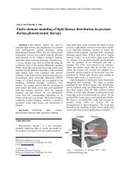
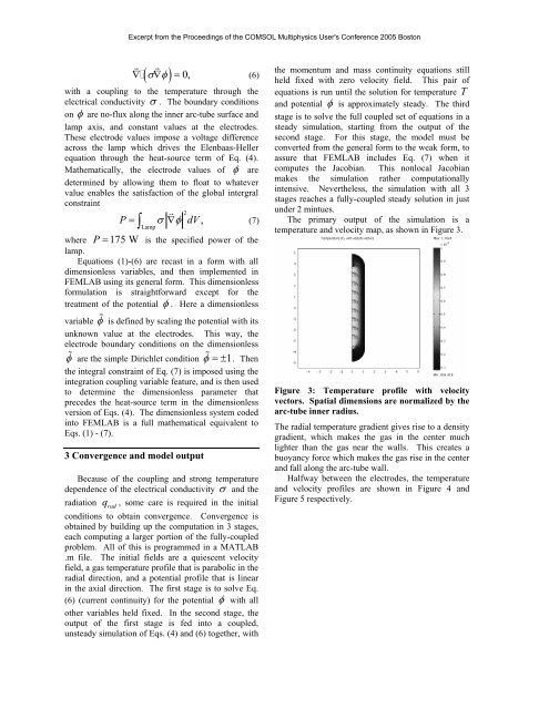
Excerpt from the Proceedings of the COMSOL Multiphysics User's Conference 2005 Bostonr r∇ ∇ =( σ φ) 0,(6)with a coupling to the temperature through theelectrical conductivity σ . The boundary conditionson φ are no-flux along the inner arc-tube surface andlamp axis, and constant values at the electrodes.These electrode values impose a voltage differenceacross the lamp which drives the Elenbaas-Hellerequation through the heat-source term of Eq. (4).Mathematically, the electrode values of φ aredetermined by allowing them to float to whatevervalue enables the satisfaction of the global intergralconstraintr 2P= σ ∇φdV,∫Lamp(7)where P = 175 W is the specified power of thelamp.Equations (1)-(6) are recast in a form with alldimensionless variables, and then implemented inFEMLAB using its general form. This dimensionlessformulation is straightforward except for thetreatment of the potential φ . Here a dimensionlessvariable φ % is defined by scaling the potential with itsunknown value at the electrodes. This way, theelectrode boundary conditions on the dimensionless% . Then% φ are the simple Dirichlet condition φ =± 1the integral constraint of Eq. (7) is imposed using theintegration coupling variable feature, and is then usedto determine the dimensionless parameter thatprecedes the heat-source term in the dimensionlessversion of Eqs. (4). The dimensionless system codedinto FEMLAB is a full mathematical equivalent toEqs. (1) - (7).3 Convergence and model outputBecause of the coupling and strong temperaturedependence of the electrical conductivity σ and theradiation qrad, some care is required in the initialconditions to obtain convergence. Convergence isobtained by building up the computation in 3 stages,each computing a larger portion of the fully-coupledproblem. All of this is programmed in a MATLAB.m file. The initial fields are a quiescent velocityfield, a gas temperature profile that is parabolic in theradial direction, and a potential profile that is linearin the axial direction. The first stage is to solve Eq.(6) (current continuity) for the potential φ with allother variables held fixed. In the second stage, theoutput of the first stage is fed into a coupled,unsteady simulation of Eqs. (4) and (6) together, withthe momentum and mass continuity equations stillheld fixed with zero velocity field. This pair ofequations is run until the solution for temperature Tand potential φ is approximately steady. The thirdstage is to solve the full coupled set of equations in asteady simulation, starting from the output of thesecond stage. For this stage, the model must beconverted from the general form to the weak form, toassure that FEMLAB includes Eq. (7) when itcomputes the Jacobian. This nonlocal Jacobianmakes the simulation rather computationallyintensive. Nevertheless, the simulation with all 3stages reaches a fully-coupled steady solution in justunder 2 mintues.The primary output of the simulation is atemperature and velocity map, as shown in Figure 3.Figure 3: Temperature profile with velocityvectors. Spatial dimensions are normalized by thearc-tube inner radius.The radial temperature gradient gives rise to a densitygradient, which makes the gas in the center muchlighter than the gas near the walls. This creates abuoyancy force which makes the gas rise in the centerand fall along the arc-tube wall.Halfway between the electrodes, the temperatureand velocity profiles are shown in Figure 4 andFigure 5 respectively.
Page 1: Excerpt from the Proceedings of the
Page 5: Excerpt from the Proceedings of the

Simulation of heat and momentum flow in a quartz mercury ... - Comsol

Create successful ePaper yourself

Delete template?

Save as template?