Linear Regression With One Predictor Variable - Jonathan Templin's ...

Chapter 1 : Linear Regression With OnePredictor VariableLecture 13October 24, 2006Psychology 790Lecture 13 Psychology 790

Today’s Lecture● Where we are going for the rest of the semester.➤ Today’s Lecture➤ ScheduleRegressionConceptsSimple LinearRegression● Simple linear regression.✦ Chapter 1 of Kutner.● Regression concepts.Wrapping UpLecture 13 Psychology 790

Our New ScheduleLecture 13 Psychology 790

Regression ConceptsLecture 13 Psychology 790

Linear Regression➤ Today’s Lecture➤ ScheduleRegressionConcepts➤ LinearRegression➤ Basic Concepts inRegression➤ Other Forms ofRegressionSimple LinearRegressionWrapping Up● We use regression analysis when we want to predict onevariable from another.● The most basic form of regression is called simpleregression:✦ We have 1 independent variable and 1 dependentvariable.✦ We are predicting a linear trend (both are continuousvariables).Y i = β 0 + β 1 X i + ǫ i● In regression, we attempt to determine the magnitude of the(typically imperfect) relationship between a set ofindependent variables and the dependent variable.Lecture 13 Psychology 790

Linear Regression➤ Today’s Lecture➤ ScheduleRegressionConcepts➤ LinearRegression➤ Basic Concepts inRegression➤ Other Forms ofRegressionSimple LinearRegression● Independent variable(s) (X): Also called the predictorvariable. The variable that we believe influences ourdependent variable.✦ Independent variables are on the right side of theequation, dependent variables are on the left side of theequation.● Dependent variable(s) (Y): Also called the response variable.The variable of interest that we want to predict.Wrapping UpLecture 13 Psychology 790

Basic Concepts in Regression➤ Today’s Lecture➤ ScheduleRegressionConcepts➤ LinearRegression➤ Basic Concepts inRegression➤ Other Forms ofRegressionSimple LinearRegressionWrapping Up● A regression model is a formal way of stating both of thefollowing:1. A tendency of the response variable (dependent) Y tovary with the predictor variable (independent) X.2. A scattering of points around some statistical relationship(in our case a line).● The two following characteristics of a regression model are:1. There is a probability distribution of Y for each level of X.2. The means of these probability distributions vary is somesystematic fashion with X.Lecture 13 Psychology 790

Other Forms of Regression➤ Today’s Lecture➤ ScheduleRegressionConcepts➤ LinearRegression➤ Basic Concepts inRegression➤ Other Forms ofRegressionSimple LinearRegressionWrapping Up● As we will see later, regression can take on many differentforms.● We can alter our simple regression in the following ways:✦ Add more than 1 independent variable.✦ Add more than 1 dependent variable.✦ Study a non-linear relationship.✦ Study relationship with categorical independent variables(ANOVA).● What if we wanted to linearly predict Y given a value of asingle variable X?✦ We use Simple Linear Regression.Lecture 13 Psychology 790

Simple Linear RegressionLecture 13 Psychology 790

Simple Linear Regression➤ Today’s Lecture➤ ScheduleRegressionConceptsSimple LinearRegression➤ The Basics➤ ImportantFeatures➤ Estimation➤ Example➤ Point Estimation➤ VarianceEstimationWrapping Up● Assume (for now) X is fixed at pre-determined levels in anexperiment - independent variable.✦ For example, we have an experiment where subjects aregiven X cups of coffee.✦ Subjects should be randomly assigned to a group drinkingeither 1, 2, 3, 4,or 5 cups of coffee.● Then we want to estimate the linear effect of theindependent variable X on the dependent variable Y .✦ For our example, we want to see how coffee drinkingaffects blood pressure.✦ Blood pressure = Y = dependent variable.Lecture 13 Psychology 790

The Basics● The linear regression model (for observation i = 1, . . .,N):➤ Today’s Lecture➤ ScheduleRegressionConceptsSimple LinearRegression➤ The Basics➤ ImportantFeatures➤ Estimation➤ Example➤ Point Estimation➤ VarianceEstimationWrapping UpY i = β 0 + β 1 X i + ε i● Don’t be confused by the Greek alphabet, this is simply theequation for a line (y = mx + b).● β 0 is the mean of the population when X is zero...the Yintercept.● β 1 is the slope of the line, the amount of increase in Ybrought about by a unit increase (X ′ = X + 1) in X.● ε i is the random error, specific to each observation.Lecture 13 Psychology 790

Important Features1. The response Y i is a random variable.➤ Today’s Lecture➤ ScheduleRegressionConceptsSimple LinearRegression➤ The Basics➤ ImportantFeatures➤ Estimation➤ Example➤ Point Estimation➤ VarianceEstimationWrapping Up2. E(ε i ) = 0 therefore E(Y i ) = β 0 + β 1 X i .3. The response term Y i varies by the error term ε i .4. σ 2 (ε i ) = σ 2 (Y i ) = σ 2 - Each probability distribution of Y hasthe same variance σ 2 .5. All error terms are uncorrelated.● Each response Y i comes from a probability distribution with:Mean:E(Y i ) = β 0 + β 1 X iVariance: Var(Y i ) = σ 2 (Y i ) = σ 2 (β 0 + β 1 X i + ǫ i ) = σ 2 (ǫ i ) ≡ σ 2● Any two responses are uncorrelated.Lecture 13 Psychology 790

Parameter Estimates● The simple linear regression model is parameterized as:➤ Today’s Lecture➤ ScheduleRegressionConceptsSimple LinearRegression➤ The Basics➤ ImportantFeatures➤ Estimation➤ Example➤ Point Estimation➤ VarianceEstimationWrapping UpY i = β 0 + β 1 X i + ǫ i● To find estimates for β 0 and β 1 there are quite a few choices:✦ So thatN∑ǫ 2 i is minimized.i✦ By making distributional assumptions about ǫ i and usingmaximum likelihood estimators.✦ So thatN∑|ǫ i | is minimized.i✦ From some guy in the hallway, or Bob Henson’s(http://www.uncg.edu/ rahenson/) Dad.Lecture 13 Psychology 790

And The Winner Is...● Finding β 0 and β 1 that minimize:➤ Today’s Lecture➤ ScheduleRegressionConceptsSimple LinearRegression➤ The Basics➤ ImportantFeatures➤ Estimation➤ Example➤ Point Estimation➤ VarianceEstimationWrapping UpN∑● Using calculus, these happen to be:∑ (Xi − ¯X)(Y i − Ȳ ) sβ 1 = ∑ y(Xi − ¯X) = r 2 xy =s x● And:iǫ 2 iβ 0 = Ȳ − β 1 ¯X∑ xy∑ x2● LS estimates are considered BLUE: Best Linear UnbiasedEstimators.● You are in luck: the LS estimators for β 0 and β 1 are also theMLEs for β 0 and β 1 when error terms are N(0, σ 2 ).Lecture 13 Psychology 790

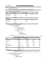
An Example of Simple Linear Regression● The following is data from an experiment where X was the number of hoursgiven for study, and Y is the score on a test.Lecture 13 Psychology 790

15-1

Example (continued)➤ Today’s Lecture➤ ScheduleRegressionConceptsSimple LinearRegression➤ The Basics➤ ImportantFeatures➤ Estimation➤ Example➤ Point Estimation➤ VarianceEstimationWrapping Up● We can tell that:✦ ∑ (X i − ¯X) 2 = ∑ X 2 i = 40✦ ∑ (X i − ¯X)(Y i − Ȳ ) = ∑ X i Y i = 30✦ ¯X = 3.0✦ Ȳ = 7.3● So:β 1 =∑Xi Y i∑ X2i= 3040 = 0.75β 0 = Ȳ − β 1 ¯X = 7.3 − (0.75 × 3.0) = 5.05● Given these estimates, the linear regression line is given by:Ŷ = 5.05 + 0.75XLecture 13 Psychology 790

Example (continued)Lecture 13 Psychology 790

Example (continued)➤ Today’s Lecture➤ ScheduleRegressionConcepts12.0010.00Test Score = 5.05 + 0.75 * XR−Square = 0.17WWWWWWWTest ScoreSimple LinearRegression➤ The Basics➤ ImportantFeatures➤ Estimation➤ Example➤ Point Estimation➤ VarianceEstimation8.006.004.00WWWWWWWWWWWWWrapping UpW1.00 2.00 3.00 4.00 5.00Hours of StudyLecture 13 Psychology 790

Example SAS Codelibname ex1 ’C:\Documents and Settings\Jonathan Templin\Desktop\Psych 790\Lectures\10_24\data’;proc gplot data=ex1.sasex1;plot y*x;run;ods html style=journal;ods graphics on;proc print data=ex1.sasex1;run;proc glm data=ex1.sasex1;model y=x /solution;run;ods graphics off;ods html close;18-1

Example (continued)➤ Today’s Lecture➤ ScheduleRegressionConceptsSimple LinearRegression➤ The Basics➤ ImportantFeatures➤ Estimation➤ Example➤ Point Estimation➤ VarianceEstimation● Ok, so now you have the parameter estimates, so what dothey mean?● Meaning of β 0Ŷ i = 5.05 + 0.75X i✦ In general, it is mean of Y when X = 0.✦ For this example, it is the mean test score when studentsdo not study for the test.✦ So, students score a 5.05 on average when they did notstudy.Wrapping UpLecture 13 Psychology 790

Example (continued)Ŷ = 5.05 + 0.75X➤ Today’s Lecture➤ ScheduleRegressionConceptsSimple LinearRegression➤ The Basics➤ ImportantFeatures➤ Estimation➤ Example➤ Point Estimation➤ VarianceEstimation● Meaning of β 1✦ In general, increase in Y for each unit increase in X.✦ For this example, the mean test score for studentsincreases by .75 for each additional hour they study.✦ So, adding an additional hour to your study time will resultin an average score of .75 points higher, two hours equal1.5 points higher, etc.Wrapping UpLecture 13 Psychology 790

Point Estimation➤ Today’s Lecture➤ ScheduleRegressionConceptsSimple LinearRegression➤ The Basics➤ ImportantFeatures➤ Estimation➤ Example➤ Point Estimation➤ VarianceEstimation● How do we estimate or predict the value of Y given a certainvalue of X.● With any probability distribution, our best estimate is themean.● How do we find the mean at a given point?● Well, E(Y i ) = β 0 + β 1 X i (use the regression equation andplug in your value of X).Wrapping UpLecture 13 Psychology 790

Point Estimation➤ Today’s Lecture➤ ScheduleRegressionConceptsSimple LinearRegression➤ The Basics➤ ImportantFeatures➤ Estimation➤ Example➤ Point Estimation➤ VarianceEstimation● Back to our example, what is the expected value on theexam for a person that studies for 4 hours?E(Y ) = 5.05 + 0.75 · 4E(Y ) = 8.05● For a person studying 4 hours, the expected score on theexam is Ŷ = 8.05.Wrapping UpLecture 13 Psychology 790

Variance Estimation➤ Today’s Lecture➤ ScheduleRegressionConceptsSimple LinearRegression➤ The Basics➤ ImportantFeatures➤ Estimation➤ Example➤ Point Estimation➤ VarianceEstimationWrapping Up● As an added note, we can also estimate the variance of Y ,σ 2 .● The long way is to compute it is by:ˆσ 2 =∑ (Yi − Ŷi) 2● The shortcut way is to use the SAS output we have (see nextslide).● You will notice on your output that you have an ANOVA table- SSE (Sum of Squares Error) is an estimate of your varianceσ 2nLecture 13 Psychology 790

Variance EstimationLecture 13 Psychology 790

Final Thought➤ Today’s Lecture➤ ScheduleRegressionConceptsSimple LinearRegressionWrapping Up➤ Final Thought➤ Next Class● Today we introducedregression - a topic we willcover for the rest of thesemester.✦ We will come to see howwe can use regression(as part of the generallinear model) toaccomplish most of ourstatistical tasks.● The simple linear regression model is easily extendable tomore complicated regression models.● We will see the types of hypothesis tests we can use forregression next time.Lecture 13 Psychology 790

Next Time● Kutner Chapter 2 (please read before class).➤ Today’s Lecture➤ ScheduleRegressionConceptsSimple LinearRegression● Inferences in Regression and Correlation.✦ Testing the regression parameters.✦ Intervals for ŶWrapping Up➤ Final Thought➤ Next ClassLecture 13 Psychology 790