Maximum Likelihood Estimation Covered This Session

Maximum Likelihood EstimationAdvanced Multivariate StatisticalMethods WorkshopUniversity of Georgia:Institute for Interdisciplinary Research inEducation and Human Development06 ‐ Maximum Likelihood EstimationCovered This Session• The basics of maximum likelihood estimation‣ The engine that drives most modern statistical methods• Additional information from MLEs‣ Likelihood ratio tests‣ Information criteria• Useful properties of maximum likelihood estimates (MLEs)‣ Missing data with ML• Adjusting MLEs for violations of assumptions06 ‐ Maximum Likelihood Estimation

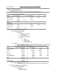
Example Data• We return to the data given in Enders (2010)‣ Imagine an employer is looking to hire employees for a jobwhere IQ is important‣ Two variables:• IQ scores• Job performance (which potentially is missing)• We will use three forms of the data:‣ Complete‣ Performance with MCAR missing‣ Performance with MAR missing06 ‐ Maximum Likelihood EstimationIQPerformance:CompletePerformance:MCARPerformance:MAR78 9 ‐ ‐84 13 13 ‐84 10 ‐ ‐85 8 8 ‐87 7 7 ‐91 7 7 792 9 9 994 9 9 994 11 11 1196 7 ‐ 799 7 7 7105 10 10 10105 11 11 11106 15 15 15108 10 10 10112 10 ‐ 10113 12 12 12115 14 14 14118 16 16 16134 12 ‐ 1206 ‐ Maximum Likelihood EstimationDescriptive StatisticsVariable Mean SDIQ 100 14.13Perf‐C 10.35 2.68Perf‐MCAR 10.60 2.92Perf‐MAR 10.67 2.79Covariance Matrix (denom = N)Complete DataIQ 189.6 19.5Performance 19.5 6.8MCAR Data (Pairwise Deletion)IQ 115.6 19.4Performance 19.4 8.0MAR Data (Pairwise DeletionIQ 130.2 19.5Performance 19.5 7.3

AN INTRODUCTION TO MAXIMUMLIKELIHOOD ESTIMATION06 ‐ Maximum Likelihood EstimationWhy Estimation is Important• In “applied” statistics courses, estimation is not discussedvery frequently‣ Can be very technical…very intimidating• Estimation is of critical importance‣ Quality and validity of estimates (and of inferences made fromthem) depends on how they were obtained• Consider an absurd example:‣ I say the mean for IQ should be 20 –just from what I feel‣ Do you believe me? Do you feel like reporting this result?• Estimators need a basis in reality (in statistical theory)06 ‐ Maximum Likelihood Estimation

Properties ofMaximum Likelihood Estimators• Provided several assumptions (“regularity conditions”) are met,maximum likelihood estimators have several goodstatistical properties:1. Consistency: the estimator converges in probability to the valuebeing estimated2. Asymptotic Normality: as the sample size increases, thedistribution of the estimator is normal (with variance given by“information” matrix)3. Efficiency: No other estimator will have a smaller standard error• Because they have such nice properties, MLEs are commonly usedin statistical estimation06 ‐ Maximum Likelihood EstimationMaximum Likelihood: Estimates Based onStatistical Distributions• Maximum likelihood estimates come from statisticaldistributions – assumed distributions of data‣ In our class, the most frequently used distribution is the multivariatenormal• We will begin our discussion with the univariate normaldistribution and expand to the multivariate normal• For a single random variable , the univariate normaldistribution is ‣ Provides the height of the curve for a value of , , and 06 ‐ Maximum Likelihood Estimation

Univariate Normal DistributionFor any value of , gives the height of the curve (relative frequency)06 ‐ Maximum Likelihood EstimationExample Distribution Values• Let’s examine the distribution values for the IQ variable‣ We assume that we know 100 and 189.6• Later we will not know what these values happen to beFor 100, 100 0.0290For 80, 80 0.010106 ‐ Maximum Likelihood Estimation

From One Observation…To The Sample• The distribution function shown on the last slide was forone observation, but we will be working with a sample‣ Assuming the sample are independent and identicallydistributed, we can form the joint distribution of the sample ,…, ⋯ 12 exp 2 2 exp 2 06 ‐ Maximum Likelihood EstimationThe Sample Likelihood Function• From the previous slide: • For this function, there is one mean ( ), one variance ( ),and all of the data • If we observe the data but do not know the mean and/orvariance, then we call this the sample likelihood function• Rather than provide the height of the curve of any value of ,it provides the likelihood for any values of and ‣ Goal of Maximum Likelihood is to find values of and thatmaximize this function06 ‐ Maximum Likelihood Estimation

Likelihood Function In Use• Imagine we know that but we do not know • The likelihood function will give us the likelihood of arange of values of • The value of whereL is the maximum isthe MLE for :• •06 ‐ Maximum Likelihood EstimationThe Log‐Likelihood Function• The likelihood function is more commonly re‐expressed asthe log‐likelihood:‣ The natural log of log log 2 exp 2 log 2 2 log 2 2 • The log‐likelihood and the likelihood have a maximum atthe same location of and 06 ‐ Maximum Likelihood Estimation

Log‐Likelihood Function In Use• Imagine we know that but we do not know • The log‐likelihood function will give us the likelihood of arange of values of • The value of whereis the maximumis the MLE for :• •06 ‐ Maximum Likelihood EstimationMaximizing the Log Likelihood Function• The process of finding the values of and thatmaximize the likelihood function is complicated‣ What was shown was a grid search: trial‐and‐error process• For relatively simple functions, we can use calculus to findthe maximum of a function mathematically‣ Problem: not all functions can give closed‐form solutions (i.e.,one solvable equation) for location of the maximum‣ Solution: use efficient methods of searching for parameter (i.e.,Newton‐Raphson)06 ‐ Maximum Likelihood Estimation

Using Calculus: The First Derivative• The calculus method to findthe maximum of a functionmakes use of thefirst derivative‣ Slope of line that is tangentto a point on the curve• When the first derivative iszero (slope is flat), themaximum of the functionis found‣ Could be a minimum – butour functions will be convex06 ‐ Maximum Likelihood EstimationFirst Derivative = Tangent LineFrom:Wikipedia06 ‐ Maximum Likelihood Estimation

The First Derivative for the Sample Mean• Using calculus, we can find the first derivative for themean (the slope of the tangent line for any value of ): • To find where the maximum is, we set this equal to zeroand solve for (giving us an ML estimate ): 06 ‐ Maximum Likelihood EstimationThe First Derivative for the Sample Variance• Using calculus, we can find the first derivative for thevariance (slope of the tangent line for any value of ): • To find where the maximum is, we set this equal to zeroand solve for (giving us an ML estimate ): 06 ‐ Maximum Likelihood Estimation

Standard Errors: Using the Second Derivative• Although the estimated values of the sample mean andvariance are needed, we also need the standard errors• For MLEs, the standard errors come from the informationmatrix, which is found from the square root of ‐1 timesthe inverse matrix of second derivatives (only one valuefor one parameter)‣ Second derivative gives curvature of log‐likelihood function• Variance of the sample mean: 06 ‐ Maximum Likelihood EstimationMAXIMUM LIKELIHOOD WITH THEMULTIVARIATE NORMAL DISTRIBUTION06 ‐ Maximum Likelihood Estimation

Maximum Likelihood for the MultivariateNormal Distribution• The example from the first part of class focused on asingle variable from a univariate normal distribution‣ We typically have multiple variables from a multivariatenormal distribution 06 ‐ Maximum Likelihood EstimationThe Multivariate Normal Distribution • The mean vector is • The covariance matrix is ‣ The covariance matrix must be non‐singular (invertable)06 ‐ Maximum Likelihood Estimation

Multivariate Normal Plot Density Surface (3D)Density Surface (2D):Contour Plot06 ‐ Maximum Likelihood EstimationExample Distribution Values• Let’s examine the distribution values for the bothvariables‣ We assume that we know 10010.35and 189.6 19.519.5 6.8• We will not know what these values happen to be in practice• The MVN distribution function gives the height of thecurve for values of both variables: IQ and Performance‣ 100 10.35 0.0052• This is an observation exactly at the mean vector –highest likelihood‣ 130 13 0.0004• This observation is distant from the mean vector –lower likelihood06 ‐ Maximum Likelihood Estimation

From One Observation…To The Sample• The distribution function shown on the last slide was forone observation, but we will be working with a sample‣ Assuming the sample are independent and identicallydistributed, we can form the joint distribution of the sample ,…, ⋯ 12 2 exp 2 exp 206 ‐ Maximum Likelihood EstimationThe Sample MVN Likelihood Function• From the previous slide: , 2 exp 2• For this function, there is one mean vector (), one covariancematrix (), and all of the data • If we observe the data but do not know the mean vector and/orcovariance matrix, then we call this the sample likelihood function• Rather than provide the height of the curve of any value of , itprovides the likelihood for any values of and ‣ Goal of Maximum Likelihood is to find values of and thatmaximize this function06 ‐ Maximum Likelihood Estimation

Likelihood Function In Use• Imagine we know that but not• The likelihood function will give us the likelihood of a range ofvalues of• The value of whereL is the maximum isthe MLE for :••06 ‐ Maximum Likelihood EstimationThe Log‐Likelihood Function• The likelihood function is more commonly re‐expressed as thelog‐likelihood:‣ The natural log of log log 2 exp 2 2 log 2 2 log 2• The log‐likelihood and the likelihood have a maximum at thesame location of and06 ‐ Maximum Likelihood Estimation

Log‐Likelihood Function In Use• Imagine we know that but not• The log‐likelihood function will give us the likelihood of a rangeof values of• The value of whereis the maximum isthe MLE for :•• 124.938506 ‐ Maximum Likelihood EstimationFinding MLEs In Practice• Most likelihood functions do not have closed form estimates‣ Iterative algorithms must be used to find estimates• Iterative algorithms begin at a location of the log‐likelihood surfaceand then work to find the peak‣ Each iteration brings estimates closer to the maximum‣ Change in log‐likelihood from one iteration to the next should be small• If models have random components (discussed later), then thesecomponents are “marginalized” – removed from equation‣ Called Marginal Maximum Likelihood• Once the algorithm finds the peak, then the estimates used to findthe peak are called the MLEs‣ And the information matrix is obtained providing standard errors for each06 ‐ Maximum Likelihood Estimation

MAXIMUM LIKELIHOOD BY MVN:SAS PROC MIXED06 ‐ Maximum Likelihood EstimationUsing MVN Likelihoods in SAS PROC MIXED• In SAS, the PROC MIXED procedure is a linear (mixed)models procedure that uses (full information) ML with themultivariate normal distribution‣ Full Information = All Data Contribute• We will come to use PROC MIXED to do multivariateanalyses for all sorts of linear models‣ MANOVA‣ Repeated Measures ANOVA‣ Multilevel models/Hierarchical Linear Models‣ (Some) Factor Models06 ‐ Maximum Likelihood Estimation

PROC MIXED: Data Setup• Data must be “stacked” or “long” formatted‣ Each measured dependent variable has its own row:06 ‐ Maximum Likelihood EstimationAn Unconditional Model In PROC MIXED• The unconditional model (where no predictors are used) willgive us ML estimates of the mean vector and covariancematrix when using PROC MIXED• The REPEATED line tells SAS that data with the same IDvariable should be treated as coming from a MVN‣ Here, there will be two variables• The CLASS line tells SAS we want to estimate a mean vector(for each ID)‣ This mean vector will be dummy coded by variable (IQ/Performance)06 ‐ Maximum Likelihood Estimation

PROC MIXED Output: Model InformationCheck # of SubjectsCheck Max #Observations per SubjectCheck # of CovarianceParameters (UniqueElements in )06 ‐ Maximum Likelihood EstimationPROC MIXED Output: Iteration History• PROC MIXED uses an iterative algorithm to find MLEs:‣ First iteration (note: uses identity covariance matrix)‣ Final iteration (note: value of ‐2*log‐likelihood = ‐2*MVN loglikelihoodvalue from slide 31)‣ Important message (if not shown, don’t trust output –not atpeak of log‐likelihood function):06 ‐ Maximum Likelihood Estimation

PROC MIXED Output:Covariance Parameters• Covariance Parameter Estimates w/SEs‣ More on the Z‐value and Pr Z later (hint: Wald Test)• SAS calls the error (residual) covariance matrixthe R matrix (in empty model ; see slide 4):06 ‐ Maximum Likelihood EstimationPROC MIXED Output: Fixed Effects• The linear model regression coefficients are called fixedeffects in the mixed models literature• Mean Performance = 10.35; Mean IQ = 10.35+89.65=10006 ‐ Maximum Likelihood Estimation

PROC MIXED Output: Type 3 Tests• Type 3 Tests of Fixed Effects is F‐ratio‣ Here is within subjects test using MANOVA unstructuredcovariance matrix assumption‣ From test: mean of IQ and Performance is significantly different• Should be! Different scales!06 ‐ Maximum Likelihood EstimationUSEFUL PROPERTIES OF MAXIMUMLIKELIHOOD ESTIMATES06 ‐ Maximum Likelihood Estimation

Likelihood Ratio (Deviance) Tests• The likelihood value from MLEs can help to statisticallytest competing models‣ Assuming none of the parameters are at their boundary• Boundary issues happen when testing some covariance parameters asa variance cannot be less than zero• Likelihood ratio tests take the ratio of the likelihood fortwo models and use it as a test statistic• Using log‐likelihoods, the ratio becomes a difference‣ The test is sometimes called a deviance testΔ2log2log log ‣ is tested against a Chi‐Square distribution with degrees offreedom equal to the difference in number of parameters06 ‐ Maximum Likelihood EstimationDeviance Test Example• Imagine we wanted to test the hypothesis that theunstructured covariance matrix in our empty model wasdifferent from what we would have if the data were fromindependent observations• Null Model: • Alternative Model:• The difference between the two models is two parameters‣ Null model: one variance estimated = 1 parameter‣ Alternative model: two variances and one covariance estimated =2 parameters06 ‐ Maximum Likelihood Estimation

Deviance Test Procedure• Step #1: estimate null model (get ‐2*log likelihood)• Step #2: estimate alternative model (get ‐2*log likelihood)06 ‐ Maximum Likelihood EstimationDeviance Test Procedure• Step #3: compute test statistic2 log log 297.0 249.9 47.1‣ Note, this is actually output in PROC MIXED• Step #4: calculate p‐value from Chi‐Square Distribution with 2degrees of freedom (I used =chidist() from Excel)‣ p‐value < 0.0001• Inference: the two parameters were significantly differentfrom zero ‐‐ we prefer our alternative model to the null model• Interpretation: the unstructured covariance matrix fits betterthan the independence model06 ‐ Maximum Likelihood Estimation

Wald Tests• For each parameter , we can form the Wald statistic:‣ (typically 0)• As N gets large (goes to infinity), the Wald statisticconverges to a standard normal distribution‣ Gives us a hypothesis test of : 0• If we divide each parameter by its standard error, we cancompute the two‐tailed p‐value from the standardnormal distribution‣ Exception: bounded parameters can have issues (variances)06 ‐ Maximum Likelihood EstimationWald Test Example• Although the Wald tests for the variance parametersshouldn’t be used, PROC MIXED computes them:• Similarly, we could test whether the mean jobperformance was equal to zero using 10.35 17.7; 0.00010.584306 ‐ Maximum Likelihood Estimation

Information Criteria• Information criteria are statistics that help determine the relative fitof a model‣ Comparison is fit‐versus‐parsimony‣ Often used to compare non‐nested models• PROC MIXED reports a set of criteria (from unstructured model)‣ Each uses ‐2*log‐likelihood as a base• Choice of statistic is very arbitrary and depends on field (I use BIC)• Best model is one with smallest value‣ Information criteria from independence model (unstructured wins):06 ‐ Maximum Likelihood EstimationMISSING DATA WITHMAXIMUM LIKELIHOOD06 ‐ Maximum Likelihood Estimation

Missing Data with Maximum Likelihood• Handling missing data in maximum likelihood is muchmore straightforward due to the calculation of the loglikelihoodfunction‣ Each subject contributes a portion due to their observations• If some of the data are missing, the log‐likelihood functionuses a reduced form of the MVN distribution‣ Capitalizing on the property of the MVN that subsets ofvariables from an MVN distribution are also MVN• The total log‐likelihood is then maximized‣ Missing data just are “skipped” –they do not contribute06 ‐ Maximum Likelihood EstimationEach Subject’s Contributionto the Log‐Likelihood• For a subject , the MVN log‐likelihood can be written:log 2 log 2 1 2 log 2‣ From our examples with missing data, subjects could either have allof their data…so their input into log uses: , , ; ; , , ‣ …or could be missing the performance variable, yielding: , ; ; 06 ‐ Maximum Likelihood Estimation

Evaluation of Missing Data inPROC MIXED• If the dependent variables are missing, PROC MIXEDautomatically skips those variables in the likelihood‣ The REPEATED statement specifies observations with the samesubject ID –and uses the non‐missing observations from thatsubject only• If independent variables are missing, however, PROCMIXED uses listwise deletion‣ If you have missing IVs, this is a potential problem‣ You can sometimes phrase IVs as DVs, though06 ‐ Maximum Likelihood EstimationAnalysis of MCAR Data with PROC MIXED• Covariance matrices from slide #4 (MIXED is closer to complete):MCAR Data (Pairwise Deletion)IQ 115.6 19.4Performance 19.4 8.0• Estimated matrix from PROC MIXED:Complete DataIQ 189.6 19.5Performance 19.5 6.8• Output for each observation (obs #1 = missing, obs #2 = complete):06 ‐ Maximum Likelihood Estimation

MCAR Analysis: Estimated Fixed Effects• Estimated mean vectors:VariableMCAR Data Complete Data(pairwise deletion)IQ 93.73 100Performance 10.6 10.35• Estimated fixed effects:• Means –IQ = 89.36+10.64 = 100; Performance = 10.6406 ‐ Maximum Likelihood EstimationAnalysis of MAR Data with PROC MIXED• Covariance matrices from slide #4 (MIXED is closer to complete):MAR Data (Pairwise DeletionComplete DataIQ 130.2 19.5IQ 189.6 19.5Performance 19.5 7.3Performance 19.5 6.8• Estimated matrix from PROC MIXED:• Output for each observation (obs #1 = missing, obs #10 = complete):06 ‐ Maximum Likelihood Estimation

MAR Analysis: Estimated Fixed Effects• Estimated mean vectors:VariableMCAR Data Complete Data(pairwise deletion)IQ 105.4 100Performance 10.7 10.35• Estimated fixed effects:• Means –IQ = 90.15+9.85 = 100; Performance = 9.8506 ‐ Maximum Likelihood EstimationAdditional Issues withMissing Data and Maximum Likelihood• Given the structure of the missing data, the standard errors ofthe estimated parameters may be computed differently‣ Standard errors come from ‐1*inverse information matrix• Information matrix = matrix of second derivatives = hessian• Several versions of this matrix exist‣ Some based on what is expected under the model• The default in SAS – good only for MCAR data‣ Some based on what is observed from the data• Empirical option in SAS –works for MAR data (only for fixed effects)• Implication: some SEs may be biased if data are MAR‣ May lead to incorrect hypothesis test results‣ Correction needed for likelihood ratio/deviance test statistics• Not available in SAS; available for some models in Mplus06 ‐ Maximum Likelihood Estimation

MAXIMUM LIKELIHOOD ESTIMATEASSUMPTIONS AND CONDITIONS06 ‐ Maximum Likelihood EstimationMaximum Likelihood Estimates: RegularityConditions• From the beginning of the lecture you may recall‣ Provided several assumptions (“regularity conditions”) are met,maximum likelihood estimators have several goodstatistical properties• Asymptotic normality of MLEs/consistency (with SEs from‐1*inverse information matrix) may not hold if some ofthe following conditions occur‣ Some parameters are on boundaries• Makes likelihood ratio/deviance test not truly Chi‐Square (instead amixture of Chi‐Squares)‣ Nuisance parameters do not increase with sample size‣ Increasing information as sample size increases06 ‐ Maximum Likelihood Estimation

Additional Assumptions• Additionally, the assumed distribution of the data must beapproximately correct• This section we discussed maximum likelihood withMVN distributions‣ If data do not follow MVN:• Estimates may be biased• Standard errors will be biased (can be adjusted to be approximate)• Other distributions can be used for maximum likelihood:‣ Binary data? Bernoulli distribution‣ Count data? Poisson distribution06 ‐ Maximum Likelihood EstimationWRAPPING UP06 ‐ Maximum Likelihood Estimation

Concluding Remarks• In this section we scratched the surface ofmaximum likelihood estimation‣ Entire courses are taught on the topic• Maximum likelihood is the most powerful and most frequentlyused estimation technique used in statistics‣ Handling missing data (MCAR or MAR) by maximum likelihood is thecurrent state‐of‐the‐art• The rest of the workshop will be devoted to statistical methodsthat use maximum likelihood• Up Next: General Linear Mixed Models andMANOVA using Mixed Models (with ML)06 ‐ Maximum Likelihood Estimation