chapter 1 general introduction - Phycology Research Group, Ghent ...

GIS-BASED ENVIRONMENTALANALYSIS,REMOTESENSING AND NICHEMODELING OFSEAWEEDCOMMUNITIESKlaasPauly

“Such was the region the Nautilus was now visiting, a perfect meadow, a close carpet of seaweed,fucus, and tropical berries, so thick and so compact that the stem of a vessel could hardly tear itsway through it.” – Jules Verne, Twenty Thousand Leagues under the Sea“What a magnificent spectacle was then outspread beneath the gaze of the travellers! The island ofZanzibar could be seen in its entire extent, marked out by its deeper color upon a vast planisphere;the fields had the appearance of patterns of different colors, and thick clumps of green indicated thegroves and thickets.” – Jules Verne, Five Weeks in a BalloonTwo quotes from a great visionary, perfectly illustrating my two passions:the biology of the seas, and looking at this from a bird’s eye perspective. I’vebeen lucky enough to combine these two passions into one study during thepast 6 years, and obviously this could not have been possible without thesupport from many, many people.A complete stranger to seaweeds prior to college, I developed akeen interest in these often disregarded organisms during my first year inBiology, unmistakably initiated by Eric. Later, the predominantly marineorientatedcourses convinced me to study zoology. However, Eric and Tommade me enthusiastic for the marine biogeographical and ecologicalresearch they were doing, and, although rather unheard of at that time in thebotany department, welcomed me as a zoologist for my master’s thesis inthe Phycology Research Group. And it didn’t stop there – thanking themfor their open-minded research vision and giving me plenty of time todevelop my own “niche” in seaweed research thereafter by hybridizing withgeography would be an understatement anyhow. Likewise, Oliviersupported me in every possible way when he took over as my supervisor,and, probably even more importantly, kept me focused and on track!Moreover, the opportunity they gave me to go on many a sampling trip andcongress is simply invaluable. And speaking of invaluable, Christelle alwaysbrilliantly solved any administrative obstacles to these trips with a big smile!The Phycology group wouldn’t be complete without the technical help andcountless fruitful and animated discussions (not just on phycology!) with myoffice buddies Heroen and first Tom, later Lennert (with our differentbackgrounds and interests we made for a very productive team I might say!),as well as Frederik, Ellen, Kenny, Aga, Ana, Frederique, Dioli, Sofie andCaroline, occasionally expanded during meetings, symposiums and the likes.I’d also like to thank the members of my PhD committee as well asanonymous article reviewers for their constructive remarks.Our research group may have been small, the many less phycologyrelateddiscussions were cheerfully joined by the protistologists Bart,Katrijn, Lander, Griet, Jeroen, Pieter, Annick, Dagmar, Annelies, Ines,Caroline, Nicolas, Els, Evelien, Jeroen, Elie, Koen, Wim, and so on, sharingour corridor.Down the corridor and downstairs, I found priceless technicaladvice to kick-start the geographical part of my research provided by Rudi,

Tony and Peter, and lately also by Geert from the Archaeology Department.Together with the people from the ground floor marine lab, I kept a broadlook on the coastal environment and enjoyed many trips to Wimereux withJoke, Jelle, Jan, Karen, Katja, Nele, Marijn, Ulrike and Ann. Many peoplealso greatly helped me out with advice, among others Bea, Dirk and Jürgen.As I spent about a year combined abroad on sampling trips andfield courses, many people were indispensible for assistance, support, helpand entertainment, among which fellow students from Roscoff andVillefranche and the students who volunteered, or sacrificed, for a master’sthesis under my auspices. My elite field crew was further populated by Yoshiin Japan and the Omani buddies: Five Oceans’ Simon, Rob, Kris, Iain andOli, as well as Barry and Ligaya who made Oman almost a second home forme, “Toxic” Tom and Else, Pieter, Michel, Ali, Mussallem and Toyota LandCruiser 4500.Throughout the years, fellow students and colleagues becamefriends, and living in a joyful city as Ghent is also guaranteed to get yousurrounded by friends who made work and life a pure pleasure. Next topeople I have already mentioned stand, in no particular order, Wolf, Pieter,Griet, Mieke, Wouter, Matthias, Maureen, Martine, Sarah, Eva, ..., theunderwater hockey gang and every single Intimate Voice, as well as theDidakites and Antwerp Flyer crew who cheered up the coastal life.Like I said in the beginning, many, many people contributed to thiswork one way or another. Not being mentioned in name here is a merehonor because you have made my life and work so much better without meeven realizing how!On top of that, next to all the years of unconditional support, mytwin-brother-lifeguard-musician Koen and brother-expert-on-road-tripmusicJan did an amazing job as field biologists in Oman after a heroic crashcourse in snorkeling, unauthorized diving, make-do Arabic, better-than-me-4WD-driving and, indeed, phycology. Eternal Respect to you, and Soetkinand Delfine whom I made temporarily husbandless! I can guarantee you avery important role in Peetje’s tough stories to your lovely kids(-to-be)!Het mag duidelijk zijn dat niets van dit hele werk mogelijk geweestzou zijn zonder de immer liefdevolle steun van Moeke, Moem en Vake, netals die van Jef en Gerda. Niemand van jullie spaarde ooit kost of moeite,bloed, zweet of tranen om mij te laten verwezenlijken waarin ik geloofde.Een warm nest in de zeebries, en een warm nest in de kempen, wie zou zichmeer kunnen wensen...An, she-who-had-to-share-her-boyfriend-with-his-“mistress”/PhD,to you I dedicate this work. You made me enjoy all-things-non-biology,laugh and dance, while enjoying yourself all-things-biology I did all along.And as if that wouldn’t do, without you both this classy book and itspredecessor would look like crappy street paper! I couldn’t dream of better!

TABLE OF CONTENTSAcronyms 1Summary 3Samenvatting 7Chapter 113General IntroductionGIS and remote sensing in a nori wrap 14Introduction 14The (r)evolution of spatial information 14Spatial data types 17GIS and remote sensing: phycological applications 18Georeferencing specimens 18Remote sensing 20Distribution and niche modeling 26Future directions and research priorities 33The quest for spatial data in seaweed biology 33Georeferencing specimens 35Remote sensing 36Distribution and niche modeling 38Aims and outline 41Author contributions 46Chapter 247Modeling the distribution and ecology of Trichosolen bloomson coral reefs worldwideAbstract 48Introduction 49Materials and methods 51Species occurrence data 51Environmental data 52ENM 53Model evaluation 55Results 56Trichosolen potential distribution 56Environmental response curves for Trichosolen on coral 57Discussion 59Supplementary material 64

Chapter 3Macroecology meets macroevolution: Evolutionary nichedynamics in the seaweed HalimedaAbstract 68IntroductionMaterials and methods6971Species identification 71Preprocessing observation data 72Species phylogeny 72Macroecological data 73Evolutionary analysis of niche characteristics 74Niche modeling procedure 76Results 77Species delimitation and phylogeny 77Evolution of niche characteristics 78Niche models at the global scale 80Niche models at the regional scale 82Discussion 83Modeling seaweed distributions 83Niche modeling vs. previous approaches 83Taxonomic caveat 83Macroevolution of the macroecological niche 84Historical perspective 84Niche conservatism 84Sources of uncertainty 85Paleobiological perspective 86Global biogeography 87Dispersal limitation 87Vicariance patterns 88Regional biogeography of tropical America 89Supplementary material 9167

Chapter 497Bio-ORACLE: a global environmental dataset for marinespecies distribution modelingAbstract 98Introduction 99Materials and methods 100Remotely sensed data 100In situ measured oceanographic data 102Pre-processing and multivariate analysis of Bio-ORACLE 103rastersCase study: Codium fragile ssp. fragile 104Results 105Case study: Codium fragile ssp. fragile 105Discussion 107Data quality 107Utility for marine SDM 109Using Bio-ORACLE for marine SDM 110Comparison to other marine environmental datasets 111Conclusions and perspectives 113Supplementary material 115Chapter 5125Spatial scale-dependent prediction in marine distributionmodeling: a case studyAbstract 126Introduction 127Material and methods 129Biotic data 129Environmental data 129Landsat data 129Bio-ORACLE data 132Distribution modeling 133Data exploration & model analysis 134Results 134Discussion 138Evaluation of Landsat-based SDM 138Technical issues relating to Landsat-based SDM 141Influence of scale on marine SDM 143Supplementary material 145

Chapter 6Mapping coral-algal dynamics in a seasonal upwelling areausing spaceborne high resolution sensorsAbstract 150Introduction 151Material and methods 153Study Area and Field Work 153Remote Sensing Datasets 153Image Preprocessing 154PROBA/CHRIS 154Landsat 7 ETM+ 155Image Processing 156Supervised bottom-type classification 156Spectral indices 157Maxent sub-pixel modeling 158Results and discussion 160Supervised bottom-type classification 160Spectral index maps 163Maxent sub-pixel modeling 166Conclusion 168149Chapter 7169Low-cost very high resolution intertidal vegetation monitoringenabled by near-infrared kite aerial photographyAbstract 170Introduction 171Material and methods 172Study area 172Kite aerial photography 173Ground truthing 174Image mosaicing and processing 175Results 178Ground truthing 178RGB image classification 178NDVI 179False-color and NIR-enhanced classifications (2011 only) 182Discussion 183Quality of the presented data 183Utility of KAP in monitoring and best practice 184

Chapter 8187General discussionSpatial information in GIS-based macroalgal studies 188General aspects of modeling macroalgal distributions 189Investigating environmental data integration and effects on 195modelingMulti-sensor mapping 197Conclusion and perspectives 199References 201Curriculum Vitae 219

ACRONYMSAUCArea Under the CurveAVHRR Advanced Very High Resolution RadiometerBEM Bioclimate Envelope ModelingBio-ORACLE Ocean Rasters for Analysis of Climate and EnvironmentBNDVI Blue-substituted Normalized Difference Vegetation IndexBRTBoosted Regression TreesCALCalciteCCDCharge-Coupled DeviceCHDK Canon Hacker Development KitCHL(-a) Chlorophyll(-a)CHRIS Compact High Resolution Imaging SpectrometerDADiffuse AttenuationDIVA Data Interpolating Variational AnalysisDNDigital NumberDOM Dissolved Organic MatterEEZExclusive Economic ZoneEGNOS European Geostationary Navigation OverlayENFA Ecological Niche Factor AnalysisENM Ecological Niche ModelingETM+ Enhanced Thematic Mapper +FAIFloating Algae IndexGAD Generalized Additive ModelsGARP Genetic Algorithm for Rule set PredictionGCPGround Control PointGEBCO GEneral Bathymetric Chart of the OceansGISGeographic Information System(s)GLM Generalized Linear ModelsGPSGlobal Positioning SystemGSDGround Sampling DistanceHSM Habitat Suitability ModelingIPCC Intergovernmental Panel on Climate ChangeITSInternal Transcribed SpacerKAPKite Aerial PhotographyKIAKappa Index of AgreementLIDAR LIght Detection And Ranging orLaser Imaging Detection And RangingMaxent Maximum entropyMCMC Markov Chain Monte CarloMERIS MEdium Resolution Imaging SpectrometerMLMaximum LikelihoodMODIS MODerate resolution Imaging SpectroradiometerMPBMicroPhytoBenthosNDVI Normalized Difference Vegetation IndexNIRNear-InfraRedNOAA National Oceanic and Atmospheric AdministrationOBIS Ocean Biogeographic Information System1

PARPCAPICPOCPROBARGBRMS(E)ROCROISALSDSDMSFMSeaWiFSSLCSMOSSSTSSUSWIRTIRTOAUAVUTMVIMVNIRWAASWOAWODWOODPhotosynthetically Available Radiation orPhotosynthetically Active RadiationPrincipal Component AnalysisParticulate Inorganic CarbonParticulate Organic CarbonPRoject for OnBoard AutonomyRed Green Blue (also used separately)Root Mean Square (Error)Receiver Operating CharacteristicRegion Of InterestSalinityStandard DeviationSpecies Distribution ModelingStructure From MotionSea-viewing Wide Field-of-view SensorScan Line CorrectorSoil Moisture and Ocean SalinitySea Surface TemperatureSmall SubUnitShort-Wave InfraRedThermal InfraRedTop Of AtmosphereUnmanned Aerial VehicleUniversal Transverse MercatorVariational Inverse MethodVisible and Near-InfraRedWide Area Augmentation SystemWorld Ocean AtlasWorld Ocean DatabaseWorldwide Ocean Optics Database2

SUMMARYSummaryMarine habitats and environments are under increasing pressure worldwide.While human activities have long been demonstrated to impact coastal andpelagic communities, these effects will probably be aggravated by globalchange. It is therefore important to gain insight in spatial and temporaldynamics and patterns of primary producers such as macroalgae. However,spatial data suitable for seaweed research have only recently becomeavailable, and marine applications in general and phycological in particularhave lagged behind on terrestrial applications in spatially explicit dataacquisition and processing. This thesis aims at presenting case studies toidentify current issues in GIS-based analysis, remote sensing anddistribution modeling of algae, while suggesting workarounds, adaptationsor solutions to these specific techniques to help answering biologicalquestions.In chapter 1, the concepts of GIS and remote sensing are introduced to thephycological community, and the current state of spatial data integration inphycological research is reviewed. The storage and dissemination of spatialmetadata is of particular concern, while this can be remedied with minimaleffort to reveal valuable information for distribution modeling studies.Promising satellite sensors have been launched or are planned to revealcoarse scale environmental information which can be used as input indistribution modeling, but satellites suitable for high resolution seaweedmapping remain underrepresented.In chapter 2, following four ephemeral monotypic green algal Trichosolenblooms on catastrophically impacted coral reefs, from which the species waspreviously unknown, we use the records together with few other occurrencedata in a niche modeling study. We aim to derive ecological anddistributional information and delineate future bloom risk areas byoverlaying the suitability map with a GIS coral reef database. A pantropicaldistribution was modeled, with several reef areas where the alga has not yetbeen recorded from delineated as bloom risk area. Response curves forchlorophyll differed markedly between blooms and non-blooms. While bothblooms and non-bloom occurrences showed a strong preference for high3

Summarytemperatures, blooms responded better to broader nutrient ranges thannon-blooms.In chapter 3, we use occurrence records and their associated sea surfacetemperature and nutrient (chlorophyll) values of extant Halimeda spp. asinput in ancestral state reconstruction techniques to infer their ancestralniche and the degree of niche conservatism. We also perform nichemodeling to compare the potential niche to the known distributions. Resultsshowed that the niche of Halimeda is conserved for tropical, nutrientdepletedhabitats, while one section of the genus invaded colder watersseveral times independently. Since known distribution ranges areconsiderably smaller than modeled potential ranges, we conclude thatrestricted geographical ranges are likely the result of dispersal limitation. Wepropose suitability hotspots in adjacent ocean basins to be targeted forfieldwork to discover sibling species.Chapter 4 aims to boost marine distribution modeling applications byproviding Bio-ORACLE, the first global marine pre-packaged uniform setof environmental variables at 9km resolution, representing differentdimensions in environmental space, freely available for download. Twentythreeraster layers were constructed based on remote sensing data productsand interpolation of in situ measurements, for which a uniform landmaskwas applied. We performed a modeling test on the invasive green algaCodium fragile subsp. fragile study which shows the predictive performance ofthe dataset by correctly predicting the current distribution.In chapter 5, a high-resolution environmental dataset for regionaldistribution modeling is assembled using Landsat 7 ETM+ imagery. Habitatlayers relating to sea surface temperature, nutrient availability and turbidityas well as a substrate layer were based on 10 mosaiced scenes to cover a2000km stretch along the coast of Oman at 60m resolution. Niche modelsfor 3 species occurring in the Arabian Sea, Gulf of Oman or both weremodeled based on Landsat-derived variables as well as cropped Bio-ORACLE variables equivalent to the Landsat information. It emerged thatfor all three species, Bio-ORACLE and Landsat-based predictions weresimilar for the Gulf of Oman with relatively little environmental variability.4

SummaryBy contrast, Bio-ORACLE showed overprediction for all three species inthe more heterogeneous Arabian Sea, with Landsat models closely reflectingpreviously known distributions for the three species in the latter region.Hence, we conclude that spatial scale effects in heterogeneous marineenvironments should be considered when designing regional distributionmodeling studies.In chapter 6, multispectral Landsat 7 ETM+ and superspectralPROBA/CHRIS imagery, both high resolution at 30m and 18mrespectively, are used in a seasonal mapping effort focusing on macroalgalstands in an upwelling-exposed area in the south of Oman. While Landsat 7benefits from a SWIR band in a vegetation index to detect surfacing,floating and intertidal algae, classification accuracy was better forPROBA/CHRIS. Classification accuracy was also generally higher in thewinter compared to the summer monsoon season, where turbid waters anddense algal stands cause bottom types to be very heterogeneous.Nonetheless, an important turnover between coral dominance in winter andalgal dominance in summer was detected. Maxent models for brown algaeand coral in the summer monsoon revealed extensive sub-pixel overgrowthof algae on coral, dominating the spectral signature of these mixed pixels.Chapter 7 presents a near-infrared enabled consumer-grade digital compactcamera mounted on a kite as an effective low-cost monitoring tool forintertidal habitats, with a focus on seaweed mapping. Using computer visionsoftware, photos were automatically aligned and a 3D terrain reconstructionwas done in order to generate an orthophotomosaic. By using a redblockingfilter in front of the lens, the camera captured blue, green and nearinfraredlight only, and these band mosaics were used to create asegmentation image. The latter was used to aid pixel training for maximumlikelihood classification. A modified normalized difference vegetation indexwas also calculated, substituting red by blue. We showed that a combinationof blue, green, near-infrared and vegetation layers as input for theclassification yielded superior results to true-color image processing. Whilenot equaling the quality of professional UAV system-based aerialphotography, this monitoring tool seems ideally suited for use in remoteareas, adverse physical conditions and developing countries.5

SummaryBased on these case studies, we presented several tools and techniques thatenhance distribution modeling and mapping power for seaweedapplications. This makes a growing body of spatially explicit informationand processing algorithms suited for the marine environment available toanswer biological questions on seaweed patterns in time and space.However, some issues would benefit from further research, such as morewidely accepted model selection and evaluation tools and knowledge onmodel parameter settings.6

SAMENVATTINGSamenvattingMariene habitats en milieus staan wereldwijd onder toenemende druk. Vanmenselijke activeiten is reeds lang aangetoond dat ze een impact hebben opkust- en zeegemeenschappen, en deze effecten zullen waarschijnlijk nogversterkt worden door global change. Om hierop in te spelen is hetbelangrijk een inzicht te verwerven in de dynamiek en patronen in ruimte entijd van primaire producenten zoals zeewieren. Ruimtelijke gegevens diegeschikt zijn voor onderzoek naar zeewieren zijn echter nog maar sinds kortbeschikbaar, en mariene toepassingen in het algemeen en op wieren in hetbijzonder hinken achterop in vergelijking met terrestrische toepassingen inruimtelijke dataverwerving en –verwerking. Deze thesis heeft tot doelcasestudies naar voor te brengen om de huidige moeilijkheden in GISgebaseerdeanalyses, teledetectie en verspreidingsmodellering van wieren aante tonen, om dan aanpassingen en oplossingen voor deze technieken aan tereiken en om biologische vraagstukken te helpen beantwoorden.In hoofdstuk 1 worden de concepten van geografische informatiesystemen(GIS) en teledetectie voorgesteld aan de algologische gemeenschap, enwordt de huidige staat van ruimtelijke data-integratie in algologischonderzoek nagegaan. Vooral de opslag en verspreiding van ruimtelijkemetadata van waarnemingen van zeewieren lijkt een probleem te vormen,terwijl daar voor de hand liggende oplossingen voor uitgewerkt kunnenworden zodat deze kostbare informatie kan aangewend worden in studiesnaar verspreidingsmodellering. Een aantal van de net gelanceerde ofgeplande satellieten zijn veelbelovend omwille van de omgevingsinformatieop globale schaal die ze beschikbaar gaan stellen, hetgeen gebruikt kanworden voor verspreidingsmodellering, maar satellieten die geschikt zijn omzeewieren in kaart te brengen met een hoge resolutie zijn nog steeds schaars.In hoofdstuk 2 gebruiken we de weinige beschikbare gegevens over hetvoorkomen van het groenwier Trichosolen om de niche ervan te modelleren,nadat het in vier gevallen een snelle, kortstondige bloei had gevormd opkoraalriffen die net beschadigd waren. We willen hiermee de ecologischekarakteristieken en de verspreiding van het wier achterhalen, enrisicogebieden voor toekomstige bloeien gaan afbakenen door de7

Samenvattingresulterende geschiktheidswaarden in een GIS over een ruimtelijke databasevan koraalriffen te leggen. Het model toonde dat het zeewier eenverspreiding over de volledige tropen kent, waarbinnen verschillendekoraalriffen van waar het wier nog niet gerapporteerd werd alsbloeirisicogebied afgelijnd werden. De gemodelleerde responscurven vanTrichosolen waren vooral verschillend voor wat betreft chlorofylconcentraties(en dus organische nutriënten) in de waterkolom. Waarnemingen van zowelbloeigevallen als niet-bloeiende populaties toonden een sterke voorkeurvoor hoge temperaturen, maar het is waarschijnlijker bloeien aan te treffenin gebieden met ver uiteenlopende nutriëntenconcentraties.In hoofdstuk 3 gebruiken we gegevens over het voorkomen en degeassocieerde oppervlaktetemperatuur van het zeewater en denutriëntentoestand (a.d.h. van chlorofyl) van de huidige soorten binnen hetgroenwiergenus Halimeda om als input te dienen voor de reconstructie vande toestand in het verleden. Zo kan de ancestrale niche bepaald worden ennagegaan worden of deze niche constant bleef in de tijd(nicheconservatisme) of niet. We maken ook nichemodellen om depotentiële niche van de huidige soorten te vergelijken met hun werkelijke(gekende) verspreiding. De resultaten toonden aan dat de niche vanHalimeda beperkt is tot tropisch, nutriëntenarm water, maar dat binnen éénsectie van het genus enkele soorten verschillende malen onafhankelijk vanelkaar zich in koude wateren zijn gaan verspreiden. Omdat de gekendeverspreidingspatronen aanzienlijk kleiner zijn dan de gemodelleerdepotentiële verspreiding, besluiten we dat de beperkte geografischeverspreiding van de huidige soorten vooral het gevolg is vandispersiebeperkingen, eerder dan aan een gebrek aan geschikte milieus. Westellen voor dat de hotspots van nichegeschiktheid die in de naburigeoceanen te vinden zijn voorrang moeten krijgen om bemonsterd te wordenmet als doel nieuwe zustersoorten te ontdekken.Hoofstuk 4 heeft tot doel mariene verspreidingsmodellering tevergemakkelijken door Bio-ORACLE voor te stellen: de eerste globale,uniform gebundelde dataset van omgevingsvariabelen op 9km resolutie, diegratis online ter beschikking staat. Deze gegevens omvatten verschillendedimensies in de omgevingsruimte en bestaan uit 23 rasterkaartlagen die8

Samenvattingsamengesteld zijn op basis van teledetectieproducten en interpolaties van insitu metingen, om daar dan op een uniforme manier landpixels in temaskeren. We hebben de dataset getest op de modellering van deverspreiding van Codium fragile subsp. fragile, een goed bestudeerde invasievegroenwiersoort. De resultaten hiervan toonden de kracht van de dataset aandoor het huidige verspreidingsgebied correct te voorspellen.In hoofdstuk 5 wordt op basis van beelden van Landsat 7 ETM+ eenhoge-resolutie dataset van omgevingsvariabelen samengesteld voor hetmaken van regionale verspreidingsmodellen. Habitatkaartlagen die verbandhouden met de oppervlaktetemperatuur van het zeewater, beschikbaarheidvan nutriënten, turbiditeit en het substraat werden samengesteld op basisvan 10 satellietbeelden die een strook van 2000km langs de kust van Omandekken met een resolutie van 60m. Nichemodellen voor drie soorten dievoorkomen in de Arabische Zee, de Golf van Oman of beide werdenopgesteld op basis van zowel de Landsatkaartlagen als gegevens uit de Bio-ORACLE dataset die verkleind werden tot het studiegebied, en waaruit diegegevens gehaald werden die equivalent zijn met de kaartlagen op basis vanLandsat. Het bleek dat de verspreiding van de drie soorten even goedgemodelleerd werden op basis van zowel Bio-ORACLE als Landsat in deGolf van Oman die gekenmerkt wordt door een lagere variabiliteit.Anderzijds vertoonden de modellen op basis van Bio-ORACLE voor allesoorten een overpredictie in de meer heterogene Arabische Zee, terwijl opLandsat-gebaseerde modellen daar net wel de gekendeverspreidingspatronen goed weergaven. We besluiten daaruit dat de resolutievan omgevingsvariabelen waarmee gewerkt wordt in de modellering een rolspeelt waarmee met name in heterogene milieus rekening gehouden moetworden bij het opzetten van modelleringsstudies.In hoofdstuk 6 worden hoge-resolutie multispectrale Landsat 7 ETM+(30m resolutie) en superspectrale PROBA/CHRIS (18m resolutie) beeldengebruikt in een poging zeewiergemeenschappen seizoenaal in kaart tebrengen in een gebied dat gekenmerkt wordt door intense opwelling, in hetzuiden van Oman. Ondanks het voordeel van de korte-golf infrarood(SWIR) band van Landsat 7 voor gebruik in vegetatie-indices ombovendrijvende en intertidale wieren te herkennen, waren de9

Samenvattingclassificatieresultaten die behaald werden met PROBA/CHRIS beeldenbeter. De nauwkeurigheid van classificaties was ook beter in de winter danin de zomer, wanneer een troebele waterkolom en dichte begroeiing doorwieren ervoor zorgen dat de bodembedekking heel heterogeen wordt.Ondanks deze moeilijkheden werd een grote omschakeling gevonden vankoraaldominantie in de winter naar zeewierdominantie in de zomer.Verspreidingsmodellen voor bruinwieren en koralen in de zomer maaktenduidelijk dat er een uitgebreide overgroei van wieren op koralen plaatsvindtop een schaal kleiner dan de resolutie van de pixels; op deze manierdomineren wieren het spectrale signaal dat van deze gemengde pixelsuitgaat.Hoofdstuk 7 stelt een eenvoudige nabij-infrarood-geconverteerde digitalecompactcamera, opgehangen aan een windvlieger, voor als een efficiëntemanier om intertidale habitats op een goedkope manier te monitoren, metde nadruk op zeewiergemeenschappen. Met behulp vancomputervisiesoftware werden de foto’s automatisch gealigneerd en werdeen 3D-reconstructie van het terrein gemaakt, wat vervolgens toeliet eenorthofotomozaïek aan te maken. Door een rood-blokkerende filter voor delens te gebruiken ontving de camera enkel blauw, groen en nabij-infraroodlicht, en deze bandmozaïeken werden dan gebruikt om een beeldsegmentatieuit te voeren waarna de hele mozaïek geclassificeerd kon worden. Eenaangepaste NDVI vegetatie-index kon ook berekend worden door de rodeband te vervangen door de blauwe. We tonen aan dat de combinatie vanblauw, groen, nabij-infrarood en de vegetatie-index betere resultatenopleverde voor classificatie in vergelijking met echte kleurenbeelden (blauw,groen, rood). Dit systeem haalt weliswaar niet de kwaliteit van camera’s aanboord van professionele onbemande vliegtuigen, maar het is wel geschiktvoor zeer afgelegen gebieden, voor gebruik in barre omstandigheden en inontwikkelingslanden.Op basis van deze casestudies hebben we verschillende methodes entechnieken aangereikt die de verspreidingsmodellering en kartering vanzeewieren op punt stellen. Daardoor komt een steeds groeiend deel vanruimtelijk expliciete informatie en verwerkingsmethodes binnen handbereikvoor gebruik in het mariene milieu en om biologische vragen over10

Samenvattingzeewierverspreidingspatronen in ruimte en tijd te beantwoorden. Hoe danook, sommige problemen blijven onopgelost; zo is er meer onderzoek nodignaar een algemeen aanvaarde vorm van modelselectie en –evaluatie en is eenbeter begrip van het aanpassen van bepaalde instellingen in hetmodelleringsproces noodzakelijk.11

Samenvatting12

CHAPTER 1GENERAL INTRODUCTIONGIS-based environmental analysis, remote sensing andniche modeling of seaweed communitiesKlaas Pauly & Olivier De ClerckAdapted from the published book chapter: Pauly K & De Clerck O (2010) GISbasedenvironmental analysis, remote sensing and niche modeling of seaweedcommunities. In: A Israel, R Einav & J Seckbach (Eds) Seaweeds and their Role inGlobally Changing Environments. Cellular Origin, Life in Extreme Habitats andAstrobiology 15, Springer Science & Business Media BV, pp 95-114

Chapter 1GIS AND REMOTE SENSING IN A NORI WRAPINTRODUCTIONIn the face of global change, spatially explicit studies or meta-analyses ofpublished species data are much needed to understand the impact of thechanging environment on living organisms, for instance by modeling andmapping species’ distributional shifts. A Nature Editorial (2008) recentlydiscussed the need for spatially explicit biological data, stating that theabsence or inaccuracy of geographical coordinates associated to every singlesample prohibits, or at least jeopardizes, such studies in any research field.In this chapter, we show how geographic techniques such as remote sensingand applications based on geographic information systems (GIS) are the keyto document changes in marine benthic macroalgal communities.Our aim is to introduce the evolution and basic principles of GIS andremote sensing to the phycological community and demonstrate theirapplication in studies of marine macroalgae. Next, we review currentgeographical methods and techniques showing specific advantages anddifficulties in spatial seaweed analyses. We conclude by demonstrating aremarkable lack of spatial data in seaweed studies to date and hencesuggesting research priorities and new applications to gain more insight inglobal change-related seaweed issues.THE (R)EVOLUTION OF SPATIAL INFORMATIONThe need to share spatial information in a visual framework resulted in thecreation of maps as early as many thousands of years ago. For instance, anapproximately 6200 year old fresco map covering the city and a nearbyerupting volcano was found in Çatal Höyük, Anatolia (Turkey). Dating backeven further, the animals, dots and lines on the Lascaux cave walls (France)are thought to represent animal migration routes and star groups, some15000 years ago. Throughout written history, there has been a steadyincrease in both demand for and quality (i.e., the extent and amount ofdetail) of maps, concurrent with the ability to travel and observe one’sposition on earth. Like many aspects in written and graphic history,however, a revolutionary expansion took place with the introduction of(personal) computers. This new technology allowed to store maps (or any14

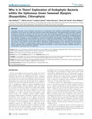
General Introductiongraphics) and additional information on certain map features in a digitalformat using an associated relational database (attribute information). It isimportant to note that the creation of GIS is not a goal in itself; instead,GIS are tools that facilitate spatial data management and analysis. Forinstance, a Nori farmer may wonder how to quantify the influence of waterquality and boat traffic on the yields (the defined goals), and use GIS astools to create and store maps and (remotely-sensed) images, and performspatial analyses to achieve these goals (figure 1).At least 30000 1 publications dating back to 1972 involve GIS(Amsterdam et al., 1972), according to ISI Web of Knowledge 2 . However,twelve years went by before the first use of GIS in the coastal or marinerealm was published (Ader, 1982), and since then only a meager 2257 havefollowed.Parallel to the evolution of mapping and GIS, the need to observeobjects without being in physical contact with the target, remote sensing,has played an important role in spatial information throughout history. In itsearliest forms, it might have involved looking from a cliff to gain anoverview of migration routes or cities. However, three revolutions haveshaped the modern concept of remote sensing. Halfway the 19 th century, thedevelopment of (balloon) flight and photography allowed to makepermanent images at a higher altitude (with the scale depending on thealtitude and zoom lens) and at many more times or places than werepreviously feasible, making remote sensing a valuable data acquisitiontechnique in mapping. Halfway the 20 th century, satellites were developedfor Earth observation, allowing to expand ground coverage. At the end ofthe 20 th century, the ability to digitally record images through the use of(multiple) CCD and CMOS sensors quickly enhanced the abilities to importand edit remote sensing data in GIS.Two kinds of remote sensing have been developed. Active remotesensing involves the emission of signals with known properties, in order toanalyze the reflection and backscatter, with RADAR (RAdio Detecting AndRanging) as the most wide-spread and best known application.1 This number is based on the search term ‘”geographic* information system*”’. The search term‘GIS’ yielded 32706 records, but an unknown number of these, including the records prior to 1972,concern other meanings of the same acronym.2 All online database counts and records mentioned throughout this chapter, including ISI Web ofKnowledge, OBIS and Algaebase records, refer to the status on July 1 st , 2008.15

Chapter 1Figure 1. Schematic overview of GIS data file types and remote sensing of a Nori farm inTokyo Bay, Japan.Passive remote sensing means recording radiation emitted or reflected bydistant objects, and most often the reflection of sunlight by objects isinvestigated. This chapter will only cover passive remote sensing and laserinducedactive remote sensing, as sound-based active sensing (RADAR,SONAR) is limited to (3D) geomorphological and topographical studies,rather than distinguishing benthic communities and their relevantoceanographic variables.The first remote sensing applications are almost a decade older thanthe first GIS publications (Bailey, 1963), and the first coastal or marine useof remote sensing appeared only few years later, starting withoceanographical applications (Polcyn & Sattinger, 1969; Stang, 1969) andfollowed by mapping efforts (Egan & Hair, 1971). Out of roughly 98500remote sensing records in ISI Web of Knowledge, however, little less than8500 cover coastal or marine topics.16

General IntroductionSPATIAL DATA TYPESAnalogous to manually drawn hard-copy maps, digitized maps (hard-copiestransferred to computers) or computer-designed maps most often consist ofthree types of geometrical features expressed as vectors (figure 1): zerodimensionalpoints, one-dimensional lines and two-dimensional polygons.For instance, a point could represent a tethered Nori platform in a bay,linked to a database containing quantitative fields (temperature, nutrients,salinity, biomass, number of active harvesting boats), Boolean fields(presence/absence of several species) and categorical fields (owner’s name,quality level label). In turn, polygons encompassing several of these pointsmay depict farms, regions or jurisdictions. Lines could either intersect thesepolygons (in case of isobaths) or border them (in case of coastal structures).Vector maps and associated databases are easy to edit, scale, re-project andquery while maintaining a limited file size.The raster data type (figure 1), also called grid or image data in whichall remote sensing data come, differs greatly from vector map data. Eachimage (whether analogously acquired and subsequently scanned, directlydigitally acquired, or computer-generated) is composed of x columns times yrows with square pixels (or cells) as the smallest unit. Each pixel ischaracterized by a certain spatial resolution (the spatial extent of a pixelside), typically ranging from 1m to 1000m, and an intensity (z-value). Theradiometric resolution refers to the number of different intensitiesdistinguished by a sensor, typically ranging from 8 bits (256) to 32 bits(4.3x10 9 ). In modern remote sensing platforms, different parts (calledbands) of the incident electromagnetic spectrum are often recorded bydifferent sensors in an array. In this case, a given scene (an image with agiven length and width, the latter also termed swath, determined by the focallength and flight altitude) consists of several raster layers with the sameresolution and extent, each resulting from a different sensor. The amount ofsensors thus determines the spectral resolution. A “vertical” profile of apixel or group of pixels through the different bands superimposed as layers,results in a spectral signature for the given pixel(s). The spectral signaturecan thus be visualized as a graph plotting radiometric intensity or pixel valueagainst band number (figure 1). The term multispectral is used for up to tensensors (bands), while hyperspectral means the presence of ten to hundreds17

Chapter 1of sensors. Some authors propose the term superspectral, referring to thepresence of 10 to 100 sensors, and reserve hyperspectral for more than 100sensors. Temporal resolution indicates the coverage of a given site by asatellite in time, i.e. the time between two overpasses. In the Nori farmexample, one or more satellite images might be used as background layers inGIS (figure 1) to digitize farms and the surroundings (based on large-scaleimagery in a geographic sense, i.e. with a high spatial resolution) or to detectcorrelations with sites and oceanographical conditions (based on small-scaleimagery in a geographic sense, i.e. with a low spatial resolution).An important aspect in GIS and remote sensing is georeferencing. Byindicating a limited number of tie points or ground control points (GCPs)for which geographical coordinates have been measured in the field or forwhich coordinates are known by the use of maps, coordinates for anylocation on a computer-loaded map can be calculated in seconds andsubsequently instantly displayed. Almost coincidentally with GIS evolution,portable satellite-based navigation devices (Global Positioning System, GPS)have greatly facilitated accurate measurements and storage of geographicalcoordinates of points of interest. In the current example, a nautical chartoverlaid with the satellite images covering the Nori farms might be used asthe source to select GCPs (master-slave georeferencing), or alternatively,field-measured coordinates of rocky outcrops, roads and humanconstructions along the coast, serving as GCPs recognizable on the (largescale)satellite images, might be used for direct georeferencing (figure 1).GIS AND REMOTE SENSING: PHYCOLOGICALAPPLICATIONSGEOREFERENCING SPECIMENSAcquiring GPS coordinates has become self-evident, with handheld GPSdevices nowadays fitting within any budget, provided that accuracyrequirements are not smaller than 10-15m. Devices capable of handlingpublicly available differential correction signals like Wide AreaAugmentation System (WAAS, covering North America), EuropeanGeostationary Navigation Overlay Service (EGNOS, covering Europe) andequivalent systems in Japan and India are slightly more expensive but offer18

General Introductionaccuracies between 1 and 10m. However, contrary to terrestrial studies(Dodd, 2011), accuracies are almost always found to be better in coastal andmarine practice, where the device would mostly be used in areas with a clearline of sight with the sky. Hence, field workers can accurately log shallowdives and snorkel tracks and revisit sampling points using consumer-gradeGPS devices mounted on buoys that are dragged along. Accuracies within1m can be obtained with commercial differential GPS systems, although thisincreases the cost and reduces mobility of field workers as a large portablestation needs to be carried along, hence restricting use on water to boats orrelatively accessible intertidal terrain. Logging GPS coordinates doeshowever not eliminate the need for textual location information, preferablyusing official names or transcriptions as featured on maps, and using ahierarchical format going from more to less inclusive entities (cf. GenBanklocality information; NCBI, 2008). This is vital to allow for error checking(see further). Several authors have recently independently andunambiguously stated that a lack of geographic coordinates linked to eachrecently and future sampled specimen can no longer be excused (NatureEditorial, 2008; Kidd & Ritchie, 2006; Kozak et al., 2008). Moreover,recommendations were made to require a standardized and publiclyavailable deposition of spatial meta-information on all used samplesaccompanying each publication, including non-spatially oriented studies.This idea is analogous to most journals requiring gene sequences to bedeposited in GenBank, whenever they are mentioned in a publication(Nature Editorial, 2008). For instance, the Barcode of Life project, aiming atthe collection and use of short, standardized gene regions in speciesidentifications, already requires specimen coordinates to be deposited foreach sequence in its online workbench (Ratnasingham & Hebert, 2007).Adding coordinates to existing collection databases can be a lot morechallenging and time-consuming. At best, a locality description string in acertain format is already provided. In that case, gazetteers can be used toretrieve geographic coordinates. However, many coastal collections aremade on remote localities without specific names, such as a series of smallbays between two distant cities. Efforts have been made to develop software(e.g. GEOLocate; Rios & Bart, 1997) combining the use of gazetteers andcivilian GPS databases to cope with information such as road names anddistances from cities. Unfortunately, most of the existing automation efforts19

Chapter 1are specifically designed for terrestrial collection databases, lacking propermaritime names, boundaries and functions. For instance, the softwareshould allow specimens to be located at a certain distance from theshoreline. For relatively small collections, coordinates can also be manuallyobtained by identifying landmarks described in the locality fields or knownby experienced field workers using Google Earth, a free GIS visualizationtool with high to very high resolution satellite coverage of the entire globe(available online at http://earth.google.com). Manually adding specimencoordinates to database records does however increase the chance of errorsin the coordinates, compared to automatically retrieving and addingcoordinates.Quality control of specimen coordinates is crucial. GIS allow foroverlaying collection data with administrative boundary maps such asExclusive Economic Zone (EEZ) boundaries, and comparing respectiveattribute tables to check for implausible locations. A common error, forinstance, involves an erroneous positive or negative sign to a coordinatepair, resulting in locations on the wrong hemisphere, on land, or in openocean. Additionally, when used in niche modeling studies, sample localitiesshould be overlaid with raster environmental variable maps, to check ifsamples are not located on masked-out land due to the often coarse rasterresolution.REMOTE SENSINGIn documenting the consequences of global change, it is crucial torepeatedly and automatically obtain baseline thematic and change detectionmaps of (commercially or ecologically critical) seaweed beds. While not ableto replace field work in detecting moderate changes in quantitativeparameters and diversity, it has long been acknowledged that remote sensingis a powerful technique to overcome numerous problems in mapping andmonitoring seaweed assemblages (Belsher et al., 1985). Accessibility ofseaweed-dominated areas can be an issue if the location is remote, and theexploration of rocky intertidal shores can be hard or even hazardous. Moreimportantly, most benthic marine macroalgal assemblages are permanentlysubmerged, restricting their exploration to SCUBA techniques. Thus,mapping and monitoring extensive stretches on a regular basis is very time20

General Introductionand resource consuming when using in situ techniques only. This sectionprovides an overview of different remote sensing approaches, withoutproviding procedural information. For hands-on information on imageprocessing techniques, see Green et al. (2000).From a technical point of view, airborne remote sensing would seemmost appropriate for seaweed mapping (Theriault et al., 2006; Gagnon et al.,2008). Light fixed-wing aircrafts are relatively easy to deploy, and sensorsmounted on a light aircraft flying at low to moderate altitudes (1000m to4000m) will typically yield datasets with a very high spatial and spectralresolution. For instance, the Compact Airborne Spectrographic Imager canresolve features measuring only 0.25m x 0.25m in up to 288 bandsprogrammable between 400nm and 1050nm in the visible and near-infrared(VNIR) light depending on the study object characteristics. Additionally, thelow acquisition altitude can result in a negligible atmospheric influence.However, light aircraft are generally not equipped with advanced autopilotcapabilities and are sensitive to winds and turbulence. It takes considerabletime and effort to geometrically correct images acquired from such anunstable platform. Altitude differences combined with roll and pitch(aircraft rotations around its 2 horizontal axes) all result in different groundpixel dimensions. Moreover, low altitude acquisitions result in a limitedswath, increasing both acquisition time (and hence expense) through the useof multiple flight transects and processing time to geometrically correct andconcatenate the different scenes. Chapter 7 in this thesis presents a tetheredlow-altitude aerial photography-based mapping of the intertidal using novelsoftware that copes with these conditions. Alternatively, a more advanced(and hence again, more expensive) and stable aircraft can acquire imagery athigher altitudes covering larger areas, but this is at the cost of spatialresolution and atmospheric influence.Overall, atmospheric and weather conditions play an important rolein aerial seaweed studies, as the aircraft and the airborne and ground crewmust be financed over an entire stand-by period in areas with unstableweather conditions (quite typical for coastal areas), as the weatherconditions at the exact moment of acquisition cannot be forecasted longenough in advance during the planning stage of the campaign.By contrast, satellites are more stable platforms that can cover muchlarger areas in one scene daily to biweekly, making these ideal monitoring21

Chapter 1resources (table 1a and 1b). However, satellite-based studies of seaweedassemblages were suffering from a lack of spatial resolution until the latenineties. Typically, seaweed assemblages are very heterogeneous due to themorphology of rocky substrates, characterized by many differences inexposure to light, temperature fluctuations, waves, grazers and nutrients ona small area. These differences result in many microclimates and –niches,creating patchy assemblages in the scale of several meters to less than ameter, while no satellite sensor resolved features less than 15m until 2000.From that year onwards, very high resolution sensors were developed andmade commercially available (table 1a), allowing for detailed subtidalseaweed mapping and quantification studies in clear coastal waters (e.g.Andréfouët et al., 2004).With the availability of more advanced sensors in the 21 st century, atrade-off between spatial and spectral resolution became apparent (figure 2)– an issue of particular relevance to seaweed studies. The trade-off situationevolved due to computer processing power and data storage capacitylimitations at the time of sensor development - often 5 years prior to launchfollowed by another 5 years of operation. This is a long time in terms ofMoore’s law (Moore, 1965), describing the pace at which computerprocessing power doubles. These historical limitations dictated a choicebetween a high spatial resolution or a high spectral resolution in currentsensors, but not both, while seaweed studies would arguably benefit fromboth. While the main macroalgal classes (red, green and brown seaweeds)are theoretically spectrally separable from each other as well as from coraland seagrass in 3 bands, this is not the case on a generic level. Additionally,information from seaweeds at below 5-10m depth can only be retrievedfrom blue and green bands due to attenuation of red and NIR in the watercolumn. Hence, the availability of several blue and green bands can increasethematic resolution and the resulting classification accuracies, and this is ofparticular value in turbid waters, characteristic of many coastal stretches. Bycontrast, the absence of a blue band combined with only one green band(see several sensors in table 1a and 1b) prevents spectral discrimination ofsubmerged seaweeds altogether and confined early remote sensing studieson seaweeds to the intertidal range (Guillaumont et al., 1993).22

General IntroductionTable 1a. Current and future spaceborne passive remote sensors apt for seaweed mapping and monitoring: technical features. Sensors are sorted ondecreasing resolution of the multispectral bands.Platform Sensor Scene Spatial Resolution Spectral ResolutionLandsat 7 ETM+ 185km x 170km 30m (60m TIR, 15m pan) 0.45-12.5µm, 6 bands + 1 thermal + 1 panEO-1 Hyperion 7.5km x 42-185km 30m 0.4-2.5µm, 220 bandsEO-1 ALI 37km x 42-185km 30m (10m pan) 0.433-2.35µm, 9 bands + 1 panPROBA CHRIS 14km x 14km 18m (36m) 0.40-1.05µm, 18 bands (63 bands), programmableTERRA ASTER 60km x 60km 15m (30m SWIR, 90m TIR) 0.52-11.65µm, 9 bands + 5 thermalSPOT 5 HRG 60km x 60km 10m (2.5m pan) 0.5-1.75µm, 4 bands + 1 panALOS AVNIR-2 70km x 70km 10m (2.5m pan) 0.42-0.89, 4 bands + 1 panFORMOSAT-2 24km x 24km 8m (2m pan) 0.45-0.9µm, 4 bands + 1 panIRS-P6 (ResourceSat-1) LISS 3-4 23.9km x 23.9km 5.8m (23.5 SWIR) 0.52-1.7, 4 bandsRapidEye (5 identical satellites) JSS 56 25km x 25km 5m 0.44-0.88µm, 5 bandsKOMPSAT-2 (=Arirang-2) 15km x 15km 4m (1m pan) 0.45-0.9µm, 4 bands + 1 panIKONOS 11.3km x 11.3km 3.28m (0.82m pan) 0.445-0.853µm, 4 bands + 1 panQuickbird 16.5km x 16.5km 2.4m (0.6m pan) 0.45-0.9µm, 4 bands + 1 panGeoEye-1 15.2km x 15.2km 1.64m (0.41m pan) 0.45-0.92µm, 4 bands + 1 panWorldView-2 16.4km x 16.4km 1.84m (0.46m pan) 0.4-1.04µm, 8 bands + 1 panPLEIADES-HR1/2 20km x 20km 2.8m (0.6m pan) 0.43-0.95µm, 4 bands + 1 panLDCM OLI 185km x 185km 30m (100m TIR, 15m pan) 0.43-12.5µm, 8 bands + 1 thermal + 1 pan23

Chapter 1Table 1b. Current and future spaceborne passive remote sensors apt for seaweed mapping and monitoring: availability, operational and quality remarks.Platform Sensor Temporal Resolution Availability Cost RemarksLandsat 7 ETM+ 16 days 1999-… Free-$ High quality earth observation data: calibration within 5%. Since the 2003 SLC failure,EO-1 Hyperion 16 days 2000-… Free-$$EO-1 ALI 16 days 2000-… Free-$$scenes are flawed with 25% gapsEO-1 flies in formation with Landsat 7’s (trailing by 1 min) to benefit from its high qualitycalibration. EO-1 has cross-track off-nadir capability. ALI is a technology verificationinstrumentPROBA CHRIS 7 days 2001-… Free Technology verification instrument; Along track +/- 55° off-nadir capability for stereo 3DimagingTERRA ASTER 16 days 2000-… $ Lack of blue band limits use to intertidal and surfacing/floating seaweeds; VNIR crosstrack 24° off-nadir and NIR backward looking capability for stereo 3D imagingSPOT 5 HRG 1-3 days 2002-… $$-$$$ Lack of blue band limits use to intertidal and surfacing/floating seaweedsALOS AVNIR-2 2 days 2006-… $ 44° off-nadir capability; Panchromatic stereo 3D imagingFORMOSAT-2 1 day 2004-… $$-$$$ Cross and along-track 45° off-nadir capability for stereo 3D imagingIRS-P6 (ResourceSat-1) LISS 3-4 5 days 2003-… $$-$$$ Lack of blue band cf. SPOT 5; 26° off-nadir capability for stereo 3D imagingRapidEye (5 identical satellites) JSS 56 1 day (combined) 2008-... $$$ Red edge band improves vegetation monitoringKOMPSAT-2 (=Arirang-2) 3 days off-nadir 2006-… $-$$ Cross-track 30° off-nadir capabilityIKONOS 3-5 days off-nadir 1999-… $$-$$$ Cross track 60° and along-track off-nadir capability for stereo 3D imagingQuickbird 1-3.5 days off-nadir 2001-… $$-$$$ Cross and along-track 30° off-nadir capability for stereo 3D imagingGeoEye-1 3-5 days off-nadir 2008-… $$$ Cross track 60° and along-track off-nadir capability for stereo 3D imagingWorldView-2 1.1-3.7 days 2009-… $$-$$$ Cross-track 40° off-nadir capability. Red edge band improves vegetation monitoring;coastal blue band improves water penetration and oceanographic observationsPLEIADES-HR1/2 1 day off-nadir (combined) 2012-… $? Planned successor in SPOT series. Capable of steering 30° off-track and viewing 43° off-nadirLDCM OLI 16 days 2013-… $? Planned successor in Landsat series. Successor of EO-1 ALI technology. coastal blue band improves waterpenetration and oceanographic observationsNote: table 1 represents the situation as of June 2011. $ = less than $500; $$ = $500-2500; $$$ = more than $2500 per 50 km² or per scene. Prices may vary according toarchived imagery or new acquisition tasks.24

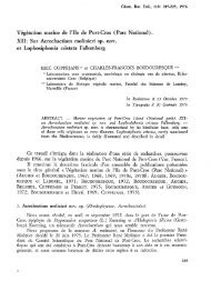
General IntroductionFigure 2. Trade-off between Log spectral resolution plotted against Log VNIR spatialresolution in current and future satellite sensors. All sensors are spaceborne, except for theairborne CASI sensor, shown here for comparison. In order to demonstrate the trade-offextremes, the panchromatic-only missions Worldview-1 and GeoEye-2 are added in thefigure but not further discussed for seaweed mapping. Likewise, the ocean color sensorsMODIS and MERIS are displayed for illustrative purposes. We consider sensors featuring aspatial resolution between 0 and 30m and a spectral resolution above 15 bands in the visibleand NIR spectrum of high value for seaweed mapping and monitoring (upper rightquadrant). We therefore recommend future satellite sensor developments towards the CASIposition, but note the position of the planned earth observation missions LDCM/OLI andPleiades along the current trade-off situation. ♦ current sensors (on which the trade-off lineis based); ■ future sensors; ▲ current sensors forming an exception to the general trade-offsituation between spectral and spatial resolution in satellite sensors.Besides the intertidal, NIR bands are useful (in combination with red) todiscriminate surfacing or floating seaweeds, and allow to discerndecomposing macroalgae, as NIR reflection decreases with decreasingchlorophyll densities (Guillaumont et al., 1997). From figure 2, it should benoted that two high spatial resolution spectral imaging sensors have beendeveloped recently, Hyperion (onboard EO-1) and CHRIS (onboardPROBA), with a spectral resolution approaching that of airborne sensors,hence forming an exception on the historical trade-off. Research by the firstauthor of this chapter suggested that CHRIS imagery can be used to mapand monitor benthic communities in turbid waters at the south coast of25

Chapter 1Oman (Arabian Sea). Intertidal green, brown and red seaweeds as well assubmerged mixed seaweed beds, coral and drifting decomposing seaweedswere discerned with reasonable accuracy during both monsoon seasons, asreported in Chapter 6 of this thesis.DISTRIBUTION AND NICHE MODELINGFor centuries, biogeographical patterns have been studied in a descriptiveway by delineating provinces and regions based on observed speciespresences and degrees of endemism, rather than quantifying and explainingthese patterns based on environmental variables (Adey & Steneck, 2001).The question as to which environmental variables best explain seaweedspecies’ niches and distributions, is however one of the most important inglobal change research. Biogeographical models based on these variablescould allow for predicting range shifts and directing field work to discoverunknown seaweed species and communities.It is widely recognized that temperature is a major forcingenvironmental variable for coastal macrobenthic communities in general andseaweeds in particular. Temperature plays a significant role in biochemicalprocesses, and generally species have evolved to tolerate only a (small)portion of the entire range of temperatures in coastal waters. Thus, it isevident that sea surface temperature (SST, often used as a proxy for watercolumn temperature in shallow coastal waters) plays a prominent role inseaweed niche distribution models. Furthermore, while temperature is oftenmeasured in a time-averaged manner (daily, monthly, yearly), it is importantto note that the timing of seasons differs globally (even within hemispheresdue to seasonal upwelling phenomena). As some seaweed species or specificlife cycles are limited by maximum and others by minimum temperatures, itis obviously essential to base models on biologically more relevantmaximum, minimum and related derived variables rather than on raw timeaveragedmeasurements.van den Hoek et al. (1990) gave an overview of how generalized orannual temperature isotherm maps could be used to explain the geographicdistribution of seaweed species in the context of global change.Adey & Steneck (2001) later described a quantitative model based onmaximum and minimum temperatures as the main variables, combined with26

General Introductionarea and isolation, to explain coastal benthic macroalgal speciesdistributions. Additionally, their thermogeographic model was integratedover time as they incorporated temperatures from glacial maxima, allowingbiogeographical regions to dynamically shift in response to two historicalstable states of temperature regimes (glacial maxima and interglacials). Inthis respect, their study is of significant value in global change research,although their graphic model outputs were not based on GIS and notstraight-forward to interpret. Moreover, using analogous or vectorisothermal SST maps, both studies suffered from a lack of resolution in SSTinput data, consequently compromising the resolution and accuracy of themodel outputs.Recently, two major studies demonstrated how seaweed distributionmodels can benefit greatly from the extensive and free availability ofenvironmental variables on a global scale through the use of satellite data.These data are not only geographically explicit and readily usable in GIS, butalso provide much more accuracy than isotherm maps due to theircontinuity. Schils & Wilson (2006) used Aqua/MODIS three-monthlyaveraged SST data in an effort to explain an abrupt macroalgal turnoveraround the Arabian Peninsula. Their results pointed to a threshold of 28°C,defined by the average of the three warmest seasons, explaining diversitypatterns of the seaweed floras across the entire Indian Ocean. They stressedthat a single environmental factor can thus dominate the effect of other,potentially interacting and complex variables. On the other hand, Graham etal. (2007) took several other variables in consideration to build a globalmodel predicting the distribution of deep-water kelps. Their study wasessentially a 3D mapping effort to translate the fundamental niche of kelpspecies, as determined by ecophysiological experiments, from environmentalspace into geographical space, based on global bathymetry,photosynthetically active radiation (PAR), optical depth and thermoclinedepth stored in GIS. The latter was based on the interpolation of verticalprofiles, while the former three variables were derived from satellite datasets(table 2).The latest advance in distribution modeling approaches concernsseveral Species’ Distribution Modeling (SDM) algorithms, also termedEcological Niche Modeling (ENM), Bioclimatic Envelope Modeling (BEM)or Habitat Suitability Mapping (HSM). While the names are often mixed in27

Chapter 1the same context, a slight difference in meaning exists (see box 1 foradditional background). Many different algorithms and softwareimplementations exist [Maxent (see box 2), GARP, ENFA, BioClim, GLM,GAD, BRT, but see Elith et al. (2006) for a review], but two fundamentalproperties are combined in these techniques, clearly separating them fromthe studies described in the previous paragraphs, which showed at most oneof these properties. Firstly, input data are a combination of a vector pointfile, representing georeferenced field observations of a species (as opposedto ecophysiological experimental data) on the one hand, and climaticvariables stored in a raster GIS on the other hand. The modeling algorithmsthen read the data out of GIS and use statistical functions to calculate therealized niche (as opposed to the fundamental niche; Hutchinson, 1957) inenvironmental space, subsequently projecting the niche back intogeographical space in GIS. Secondly, instead of a binary identification ofsuitable and unsuitable areas, ENM output is a continuous probabilitydistribution, which makes more sense from a biological point of view.Table 2. Current environmental variables retrievable from selected satellite data on a globalscale.Variable Source Resolution (level 3) AvailableSea Surface Temperature (SST) NOAA/AVHRR/1-3 4-9km (2-5arcmin) 1985-…Terra/MODIS 4km (2arcmin) 2000-…Aqua/MODIS 4km (2arcmin) 2002-…Chlorophyll-a concentration (CHL) SeaWiFS 9km (5arcmin) 1997-2011Envisat/MERIS 9km (5arcmin) 2002-…Terra or Aqua/MODIS 4km (2arcmin) 2000-…Photosynthetically active Radiation (PAR) SeaWiFS 9km (5arcmin) 1997-2011Terra or Aqua/MODIS 4km (2arcmin) 2000-…Diffuse Attenuation (DA) SeaWiFS 9km (5arcmin) 1997-2011Terra or Aqua/MODIS 4km (2arcmin) 2000-…Dissolved Organic Matter (DOM) SeaWiFS 9km (5arcmin) 1997-2011Terra or Aqua/MODIS 4km (2arcmin) 2000-…Particulate Organic Carbon (POC) SeaWiFS 9km (5arcmin) 1997-2011Terra or Aqua/MODIS 4km (2arcmin) 2000-…Particulate Inorganic Carbon (PIC) SeaWiFS 9km (5arcmin) 1997-2011Terra or Aqua/MODIS 4km (2arcmin) 2000-…Surface winds QuikSCAT/SeaWinds 25-110km 1999-2009MetOp-A/ASCAT 12.5-25km 2006-…SAC-D/Aquarius 110km (1arcdegree) 2011-…Salinity SAC-D/Aquarius 110km (1arcdegree) 2011-…28

General IntroductionBox 1. Niches and niche modeling(after Peterson, 2006; Pearson, 2007; Soberón, 2007 and Colwell & Rangel, 2009)Species’ niches have been described in various ways since Grinnell’s first definition.The Grinnellian niche can be defined by fundamentally non-interacting habitatvariables and abiotic environmental conditions on broad scales (so-calledscenopoetic variables), relevant to understanding coarse-scale ecological andgeographic properties of species. The Eltonian niche focuses on biotic interactionsand resource-consumer dynamics essentially acting at local scales (so-calledbionomic variables). Grinnell and Elton viewed these niche concepts as an abstractset of characteristics belonging to a certain place in geographical space. Bycontrast, the Hutchinsonian niche is viewed as a multidimensional volume inhyperspace defined by axes consisting of conditions and resources, attributed to aspecies or population. The fundamental niche is then the full set of conditionsunder which a species can exist, while this is often constrained by speciesinteractions and/or dispersal limitations to the realized niche. In this concept, aspecies’ niche defined in environmental space can hence be translated togeographical space and vice versa. This duality forms the basis for ecological nichemodeling, as shown below.The diagram above illustrates how a hypothetical species distribution model maybe fitted to observed species occurrence records (Pearson, 2007). A modelingtechnique is used to characterize the species’ niche in environmental space by29

Chapter 1relating observed occurrence localities to a suite of environmental variables.Notice that, in environmental space, the model may not identify either the species’occupied niche or fundamental niche; rather, the model identifies only that part ofthe niche defined by the observed records. When projected back into geographicalspace, the model will identify parts of the actual distribution and potentialdistribution. For example, the model projection labeled 1 identifies the knowndistributional area. Projected area 2 identifies part of the actual distribution that iscurrently unknown; however, a portion of the actual distribution is not predictedbecause the observed occurrence records do not identify the full extent of theoccupied niche (i.e. there is incomplete sampling). Similarly, modeled area 3identifies an area of potential distribution that is not inhabited (the full extent ofthe potential distribution is not identified because the observed occurrence recordsdo not identify the full extent of the fundamental niche due to, for example,incomplete sampling, biotic interactions, or constraints on species dispersal).Inherently, biotic samples from the physical world yield occurrence records in therealized part of a species' niche, as opposed to its fundamental niche, sinceknowledge on all species interactions cannot be obtained in regular samplingcampaigns and absence of interactions cannot be assumed. Moreover, it is veryhard to generate raster layers accounting for biotic interactions such as grazing,which would reflect a species' Eltonian niche. Hence, all the modeling case studiesin this thesis are exclusively based on abiotic (so-called scenopoetic) variables,defining the (realized) Grinnellian niche (Colwell & Rangel, 2009; Rödder &Engler, 2011). It is important to note that although Eltonian niche factors areresponsible for confining a species to its realized niche within its fundamental(Grinnellian) niche and that although exactly those Eltonian variables are notincluded in most niche modeling approaches, the modeled niche is still part of therealized niche because of the inherent input sample characteristics. This concept isespecially important for macroalgae, because in many cases (for instance, on coralreefs), the only responsible factor for local absences (or lack of occurrence data)may be grazing pressure.In the literature, the terms niche modeling, bioclimate envelope modeling, habitatsuitability modeling and species distribution modeling are often mixed or useddifferently in a range of contexts and goals. One distinction is sometimes madebetween presence-only modeling techniques, which have been referred to as nicheor envelope modeling, and modeling techniques using actual presence and absencedata, often termed distribution or suitability modeling. In the framework of thisthesis, a scale- and purpose-related definition would be more appropriate. Whenmodeling in a broad biogeographic context where environmental variables on aglobal scale are considered and issues of dispersal capacity play a role, ecologicalniche modeling would be the more appropriate term. By contrast, distribution orsuitability modeling focuses on a much finer scale, where dispersal is not thelimiting factor and species interactions would be more important. As such,Chapters 2 and 3 would be niche modeling studies, with Chapter 4 expanding thedimensions of variables that can be included, while Chapters 5 and 6 would bemore concerned with actual distribution and suitability modeling (although asexplained earlier, bionomic variables are not included). However, when relating toother studies, a strict distinction cannot be maintained.30

General IntroductionContinuous probability maps may then be converted to binary maps usingarbitrary thresholds. Additionally, ENM algorithms typically use severalstatistics to pinpoint the most important environmental variable in terms ofmodel explanation, giving its percent contribution to the model output.Also, response curves can be calculated for the different variables, definingthe niche optima.However, care must be taken to restrict model input to uncorrelatedenvironmental variables to obtain valid results. With a growing availability of(global, gridded) environmental datasets which are often correlated orredundant, a data reduction strategy should be considered. One mayperform a species-environment correlation analysis or ordination to make afirst selection of relevant variables and perform a subsequent Pearsoncorrelation test between environmental variables to get rid of redundantinformation. Alternatively, spatial principal component analysis (PCA, seebox 2) may be performed to obtain uncorrelated variables, using PCAcomponents as input variables (Verbruggen et al., 2009), although resultingvariable contributions and response curves might be hard to calculate backto original variables.Box 2. Spatial techniquesMaxent distribution modeling algorithm (after Pearson, 2007)Maxent is a general-purpose method for characterizing probability distributionsfrom incomplete information. In estimating the probability distribution defining aspecies’ distribution across a study area, Maxent formalizes the principle that theestimated distribution must agree with everything that is known (or inferred fromthe environmental conditions where the species has been observed) but shouldavoid making any assumptions that are not supported by the data. The approach isthus to find the unique probability distribution P(x) of maximum entropy (thedistribution that is most spread-out, or closest to uniform) subject to constraintsimposed by the information available regarding the observed distribution of thespecies and environmental conditions across the study area.i ⋅ fiieP x = = 1)Zn∑ c( x)( , with c = scaling constants and Z = regularization parameterIn the above equation, f i (x) denote functions of environmental variables and theirinteractions terms (so-called features). Features can take several forms, allowing tofit more or less complex models by combining features as exemplified in the figurebelow. More occurrence records are needed to fit increasingly complex functions.31

Chapter 1The Maxent method does not require absence data for the species being modeled;instead it uses background environmental data for the entire study area. Themethod can utilize both continuous and categorical variables and the output is acontinuous prediction (most commonly depicted as logistically scaled relativesuitability from 0 to 1). The freely available software implementation developed byPhillips et al. (2006, 2008, 2009, to which the reader is referred for furthermathematical details) also calculates a number of alternative thresholds to convertthe continuous probability distribution to discrete maps, computes modelvalidation statistics, and enables the user to run a jackknife procedure to determinewhich environmental variables contribute most to the model prediction. Maxenthas been shown to perform well in comparison with alternative methods (Elith etal., 2006). One drawback of the Maxent approach is that it uses an exponentialmodel that can predict high suitability for environmental conditions that areoutside the range present in the study area (i.e. extrapolation). To alleviate thisproblem, when predicting for variable values that are outside the range found inthe study area, these values can be set (or ‘clamped’) to match the upper or lowervalues found in the study area. Alternatively, extrapolation can be used to identifypotential suitable areas under new climate scenarios.Spatial PCA (after Clark Labs IDRISI manual)Principal Component Analysis (PCA) is a linear transformation technique relatedto Factor Analysis. Given a set of image bands, PCA produces a new set of images,known as components that are uncorrelated with each other and explainprogressively less of the variance found in the original set of bands. Bothstandardized and unstandardized principal component analyses can be performed.In the standardized case, the correlation matrix is used for input rather than theusual variance/covariance matrix.PCA has traditionally been used in remote sensing as a means of data compaction.For a typical set of raster layers covering the same area, it is common to find thatthe first two or three components are able to explain virtually all of the originalvariability in the pixel values. Later components thus tend to be dominated bynoise effects. By rejecting these later components, the volume of data is reducedwith no appreciable loss of information.DIVA interpolation (after Troupin et al., 2010)Data-Interpolation Variational Analysis (DIVA) is an implementation of theVariational Inverse Method (VIM). It is a geostatistical approach to theinterpolation of point data to gridded climatological fields, allowing theconsideration of coastlines and bottom topography without additionalparameterization, and has a numerical cost almost independent on the number of32

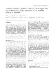
General Introductionobservations. Moreover, only a few parameters need to be determined, which isdone in an objective way. The algorithm is able to deal with a great number ofindividual data, without needing to work with averaged values or data bins. It alsogenerates coherent error maps, while the computational time required for bothclimatological and error maps is kept to a reasonable level, allowing routine runson several depth levels. For elaborate mathematical details, the reader is referred toTroupin et al. (2010).Pauly et al. (2009) applied preliminary ENM using Maxent (Phillips etal., 2006; see box 2) to gain insight in worldwide blooms of the siphonousgreen alga Trichosolen growing on physically damaged coral (figure 3). Acorrelation analysis was applied to identify the two least correlatedbiologically meaningful variables derived from SST and CHL (based onmonthly datasets), adequately describing the position and extent of thedistribution in environmental space. The model delineated the potentialglobal distribution of Trichosolen occurring on coral based on a 95% trainingconfidence threshold, including areas where the bloom had previouslyoccurred. This allowed identifying areas with a high potential risk for futureblooms based on environmental response curves. For instance, the responsecurve for the average of the three warmest months [included as a variablebased on the conclusions of Schils & Wilson (2006)] shows that Trichosolenpopulations are only viable above 22°C, but only environments above 28°Care likely to sustain blooms. Chapter 2 of this thesis presents this approachmore elaborately.FUTURE DIRECTIONS AND RESEARCH PRIORITIESTHE QUEST FOR SPATIAL DATA IN SEAWEED BIOLOGYIn its simplest form, “spatially explicit” seaweed data would refer to theavailability of georeferenced species occurrences. While we discussed thepractice of georeferencing and dissemination of spatially explicit seaweeddata in depth in the second section of this chapter, we briefly show a coupleof examples to demonstrate the dramatic state of the current availability ofthis information. For instance, looking at a random Nori species, Porphyrayezoensis Ueda, AlgaeBase (Guiry & Guiry, 2008) mentions 13 references tooccurrence records throughout the northern hemisphere.33

Chapter 1Figure 3. (a) A Pseudobryopsis/Trichosolen (PT) bloom on physically damaged coral. (b)Worldwide occurrence points of PT on coral. (c) Environmental grids used for modeltraining in Maxent. (d) Relative importance of each variable in the model as identified by thealgorithm. (e) Response curve of PT to the average of the three warmest months. (f) Binaryhabitat suitability map for PT. The grey (blue) shade represents suitable environment, whilethe dark (red) shade along the coast delineates bloom risk areas.By contrast, the Ocean Biogeographic Information System (OBIS, an onlineintegration of marine systematic and ecological information systems;Costello et al., 2007) contains no P. yezoensis records. Another randomexample, the siphonous (sub)tropical green alga Codium arabicum Kützingillustrates this further: out of 55 direct or indirect occurrence references inAlgaebase, 17 are georeferenced in OBIS. However, two of the specimenswrongly have zero longitudes, hence locating the records some 400kminland from the coast of Ghana, instead of at the Indian coast. Five out ofthe 17 are recorded to no better than 0.1 degree in both longitude andlatitude, making their position uncertain within up to 120km². Fifteen out ofthe 17 make no mention of the collector’s name or publication, preventingto check the integrity of the identification. Eleven lack sub-country levellocality name information, and none mention sub-state locality names,making it impossible to verify geographical coordinates through the use ofgazetteers.34

General IntroductionIf the amount of coastal or marine publications using GIS, mappingor remote sensing can be called minimal, averaging 8% of the totalpublications using these geographic techniques as previously shown, theproportion of these records mentioning seaweeds or macroalgae isstatistically speaking barely existing, attaining 0.5-1% of the spatial marinestudies. Studies investigating the other two best-known benthic marinecommunities, coral (reefs) and seagrasses, constitute up to 10%, while theremainder covers (in no particular order) mangroves and other supratidalcoastal communities and structures, coastal or marine topography andgeomorphology or nautical issues. Some of the reasons accounting for thisdisproportion are obvious: for a start, relatively few investigate seaweeds.However, out of 12074 studies mentioning seaweeds or macroalgae in ISIWeb of Knowledge, a potential 7279 in the fields of ecology, biogeography,phylogeography or ecophysiology could benefit from some sort of spatialexplicit information, while only 177 (2.5%) actually mention to do so intheir title, abstract or keywords. Other problems concern the nature ofseaweed communities: while coral reefs and seagrass meadows usually formlarge and relatively homogenous assemblages, seaweeds are spatially andspectrally very heterogeneous. This is particularly difficult to cope with inremote sensing studies, already challenged by the properties of the watercolumn in comparison to terrestrial vegetation studies.GEOREFERENCING SPECIMENSPrevious sections of this chapter demonstrate the need to prioritize thestandardization of disseminating and linking geographical seaweed specimeninformation. Investigating the consequences of global change requires theavailability of correct and complete global datasets. Therefore, we supportthe requirement of the dissemination of sample coordinates not only fromgeographically oriented studies, but from every study using in situ sampledseaweeds, to allow for informative and accurate meta-analyses. Coordinatepairs should be deposited in already existing global biodiversity databasessuch as OBIS, but minimal geographic accuracy and complete specimeninformation including collector’s name should be required in order to allowvigorous quality control. Additionally, the geodetic datum in whichcoordinates are shared should be part of this standardization effort.35

Chapter 1Positional data recorded in a local datum by national institutions ororganizations are hard to translate correctly to global projections. Hence, werecommend the use of WGS-84, the default global datum on consumergradeGPS devices.The use of global biodiversity databases as a main depositing centrefor specimen coordinates rather than dedicated seaweed databases alsoopens perspectives to investigate potential correlations between seaweedand faunal distribution shifts in response to global change. However, itshould also be investigated how general geographical biodiversity databasessuch as OBIS could be related to and synchronized with specific databasessuch as Algaebase and GenBank to optimize the dissemination of all kindsof specimen information.REMOTE SENSINGNo significant time gap exists between the development anddeployment of airborne sensors; due to an optimal use of the most recenttechnologies, airborne sensors thus represent the best technicalcharacteristics desirable for seaweed mapping to date. As time goes on, themost recent satellite sensors can benefit from the evolution in technologiesto more closely resemble the properties of airborne sensors. Vahtmäe et al.(2006) used a simulation study to demonstrate that submerged seaweeds inturbid coastal waters could well be mapped using hyperspectral satellitesensors like CHRIS and Hyperion, featuring 10nm wide bands in the visualwavelengths. However, they also postulated a signal-to-noise ratio of 1000:1,an image quality not met by these existing sensors. It is thus vital that similarnew hyperspectral, very high resolution satellite sensors should bedeveloped for seaweed mapping and monitoring in the framework of globalchange research. Similarly, studies on seagrass meadows have shown thatspectral separability on the species level becomes problematic on depthsgreater than 3 m due to lack of combined very high spatial and spectralresolutions, and best results to date were achieved using airbornehyperspectral sensors that do meet these requirements (Phinn et al., 2008).Ferwerda et al. (2007, also including a review of seagrass mapping studies)suggest a workaround to the lack of suitable sensors for seagrass mappingby using environmental information such as suspended sediment, water36

General Introductionconstituents, nutrient concentration and temperature that can be retrievedfrom multiple current sensors to model seagrass productivity, rather thandirectly mapping it. However, this approach is not directly applicable toseaweed mapping because of the less clear relationships between thoseenvironmental factors and seaweed growth and survival. For directmapping, Phinn et al. (2008) also recommend using imagery with both veryhigh spatial (< 5 m) and spectral resolution. By contrast, figure 2 shows thatplanned sensors for the next years follow the historical trade-off towardsmultispectral very high resolution systems. Nowadays, this seems to bemotivated by two elements: the huge thrust for coral reef research, in whichmacroalgae are often lumped into one or few functional classes and spatialresolution is considered more important than spectral resolution, anddisaster event monitoring, focusing on a near-one day site revisiting timethrough the use of extensive off-nadir or off-track pointing capabilities(table 1b).The latter technique also generates huge amounts of data, adding a newdimension to the historical trade-off situation: current data storagecapacities allow for two image characteristics out of three (spectral, spatialand temporal resolution) to be optimized, but not all three. Unfortunately,no significant thrust seems to exist in order to develop sensors ideallysuitable for large-scale algal mapping and monitoring to date, explaining thecharacteristics of the missions in development. As a means to deal with thelack of very high resolution hyperspectral imagery, efforts have been madeto combine the information from several sensors with differentcharacteristics into one dataset. This is analogous to pan-sharpeningtechniques, which use the high spatial detail of a panchromatic band tospatially enhance the multispectral imagery from the same sensor (see alsofigure 2). Although useful in current conditions, we suspect these techniquesto become less important as more advanced sensors would be developed,since processing information from one sensor evidently is less time- andresource-consuming and more accurate than using multi-sensorinformation.Light-based active remote sensing (known as LIDAR, LightDetection And Ranging) involves the emission of laser pulses with a knownfrequency and subsequently detecting fluorescence in certain wavelengths.Kieleck et al. (2001) proved this technique to be successful in discerning37

Chapter 1submerged green, brown and red seaweeds in lab conditions. Mazel et al.(2003) used a similar prototype in-water laser multispectral fluorescenceimaging system to map different coral reef bottom structures, includingmacroalgae, on a 1cm resolution. Airborne laser imaging has been usedextensively to provide very high resolution imagery in terrestrial applicationssuch as forestry. In the marine realm, its applications are mostly limited toin-water (boat-mounted) transect mapping strategies, although furtherresearch to develop aerial systems could prove useful to obtain very highresolution imagery of individual seaweed patches, e.g. to map the spreadingof macroalgae on coral reefs.DISTRIBUTION AND NICHE MODELINGPresence-only data are mostly inherent to seaweed niche distributionmodeling due to sampling locality bias (caused by difficulty of coastal andsubmerged terrain access), small sizes or seasonally microscopic life stagesof seaweed species, or cryptic species. Under the title of Species’Distribution Modeling, Pearson (2007) published a general manual including(presence-only) niche modeling, mostly based on Maxent. However, themanual is based on terrestrial experiences, as niche modeling algorithmshave rarely been applied to seaweed distribution to date, and some issuescharacteristic of marine benthic niche modeling are not elaborated. Forinstance, there are more global environmental GIS data available for theterrestrial realm compared to the marine environment. Table 2 lists marineenvironmental variables currently available from global satellite imagery,along with data that will become available in the near future. Especiallyglobally gridded, remotely sensed salinity data have only recently becomeavailable. Other variable datasets (pH, nutrients, salinity, turbidity, etc.) mayalso be compiled from the interpolation of in situ data, e.g. from theWorldwide Ocean Optics Database (Freeman et al., 2006) or the WorldOcean Database (NOAA, 2008). These data, consisting of vertical profiles,can be advantageous for 3D modeling, but the interpolation techniquesnecessary to obtain gridded maps may be challenging. An attempt to kickstartthis integration of satellite data and in situ data interpolated using DIVAis presented in Chapter 4 in this thesis (see box 2). Furthermore, globalchange climate extrapolations resulted in the production of low resolution38

General Introductionglobal gridded maps of environmental variables for future scenarios in theterrestrial realm as well as the marine realm, distributed by theIntergovernmental Panel on Climate Change (IPCC). The projection ofcalculated niches on future distributions can greatly enhance ourunderstanding of global change consequences, and it is therefore crucial thatfuture research is aimed at composing similar gridded maps of futurescenarios for marine environmental variables. More research should also beaimed at setting model parameters to account for spatial autocorrelation andclustering of species occurrence data. Lastly, model validation and outputcomparison statistics are under scrutiny in recent literature (e.g. Peterson etal., 2008), and more research is needed to agree on the best statistics suitablefor marine data.Modeling on a local scale allows for including high-resolutionenvironmental variables that are not available for the entire globe. This isparticularly the case where environmental variables not available fromsatellite data have been measured in situ and can be interpolated locally. Inother cases, one or several (very) high resolution satellite scenes can be usedto provide substrate data, not relevant on a global scale with 1km griddedenvironmental variables. For instance, De Oliveira et al. (2006) includedsubstrate, flooding frequency and wave exposure to model the distributionof several intertidal and shallow subtidal brown seaweeds along a 20kmcoastal stretch in Brittany, France. Thus, it can be expected that multiscalemodeling approaches will gain importance in the near future. A comparisonbetween models based on equivalent coarse- and fine-resolutionenvironmental data is presented in Chapter 5.While human-induced effects on habitats are thought to drive shorttermspecies dynamics, it is often stated that global climate change willinfluence the capacity of alien species to invade new areas on a medium tolong term. Range shifts of individual species in an assemblage under climatechange are based on largely the same processes driving the spread of alienspecies. Hence, the two can be addressed using the same approach (Thuilleret al., 2007). Although very complex processes are involved, the geographiccomponent of species’ invasions can be very well predicted using nichemodeling techniques (Peterson, 2003). Once a comprehensive marineenvironmental dataset is compiled, invaded areas and areas at risk ofinvasion can be successfully predicted based on the native niche of alien39

Chapter 1species (Pauly et al., 2009; Peterson, 2005), although Brönnimann et al.(2007) warn that a niche shift may occur after invasion. Nevertheless, nichemodeling approaches are promising in future research of seaweeds’ rangeshifts and invasions. Verbruggen et al. (2009) also applied niche modelingtechniques to unravel the evolutionary niche dynamics in the green algalgenus Halimeda, concluding that globally changing environments may allowcertain macroalgae to invade neighboring niches and subsequently to form adivergent lineage. They also used Maxent to identify key areas to be targetedfor future field work in search for new sister species – an application inbiodiversity considered important in the light of global change. Thisapproach is outlined in detail in Chapter 3 in this thesis.To date, seaweed assemblages have often been characterized usingquantitative vegetation analyses and multivariate statistics in order todelineate different community types and to establish the link betweenenvironmental variables and communities. With quickly developing nichemodeling algorithms now regarded as the most advanced way to accomplishthe latter, community niche modeling will be of particular value in globalchange-related seaweed research in the coming years. Ferrier & Guisan(2006) defined three ways to predict the niche of communities as a whole,rather than the niches of individual species. The assemble-first, predict-laterstrategy seems the most promising for seaweed data, since existing floristicdata have often been statistically assembled into communities. We suggestthat prioritizing the development of community niche modeling algorithmscan greatly speed up our insight in seaweed community response to futureclimate change.40

AIMS AND OUTLINEGeneral IntroductionThe general aim of this thesis is to investigate the applicability of severalspatially explicit data acquisition and processing techniques that have beendeveloped and used to map and predict the distribution of mainly terrestrialspecies to the study of seaweeds. In order to identify hands-on problemsrelated to applying these techniques in the marine realm in general andseaweeds in particular, we present case studies (see box 3 for an outline ofthe species discussed in this thesis), rather than theoretical, experimental orsimulation approaches. We suggest workarounds, adaptations andextensions to the existing methods to optimise the performance ofdistribution or niche modeling (chapters 2-5) and mapping (chapters 6-7) ofmarine species. Our goal is to show how results from these spatially explicitanalyses add new insights in the distribution and ecology of macroalgalspecies and communities, and how they can be used in future monitoringprojects.In chapter 2 we investigate the use of Maxent niche modeling to predict thepotential distribution of the green algal genus Trichosolen and to deriveecological triggers of global ephemeral blooms of the species on impactedcoral reefs. The aim is to complete scarce knowledge on the distribution andecology of this genus characterized by a partly microscopic life cycle and todelineate potential future bloom risk conditions and areas.In chapter 3 we present an application of macroecological niche modelingin a macroevolutionary context. We use GIS to retrieve environmentalinformation for georeferenced records of extant species, and use these dataas input in an ancestral state reconstruction to infer ancestral niches. Nichemodeling using Maxent is applied to compare known distributions withpotential distributions in order to evaluate speciation scenarios and todelineate areas for potential discoveries of sister species.Chapters 2 and 3 clearly demonstrate that a lot of effort in marine nichemodeling is put in the compilation of (global) marine environmental data.Therefore, chapter 4 aims to boost marine distribution and niche modelingapplications by presenting the first comprehensive standardized and41

Chapter 1uniform global marine environmental dataset, readily downloadable andusable for predictive studies. We present the methods used to integrateglobal remote sensing products and oceanographic data obtained byinterpolation of in situ measurements. Additionally, we demonstrate globalapplicability through a case study of the invasive green alga Codium fragilesubsp. fragile, predicting its potential spread.While chapters 2 to 4 focus on the global scale, chapters 5 and 6 show theapplicability and caveats of distribution modeling approaches on a regionaland local scale. In chapters 6 and 7, local mapping techniques are presented.In chapter 5, we focus on regional processes by comparing Maxentdistribution models for three key macroalgal species with previouslycharacterized differing distribution patterns along the coast of Oman, wheretwo seas with distinct environmental characteristics border each other with asharp biogeographical turnover. Moderate resolution models are based on acropped subset of the macroecological data presented in chapter 4. Theseare then compared to models based on genuine high-resolutionmacroecological and habitat layers derived from 10 mosaiced Landsat 7ETM+ scenes. First, we assess the potential of Landsat imagery as a novelenvironmental data source for regional marine distribution modeling.Second, we evaluate the influence of differences in spatial scale betweenboth environmental datasets on model outcomes in different environments,and compare our results to outcomes from similar terrestrial studies.In chapter 6, we investigate the feasibility of satellite-based local shallowhabitat mapping, with a focus on discerning macroalgal communities, toassess temporal turnover in a highly seasonal environment. To this end, wecompare high-resolution multispectral Landsat 7 ETM+ imagery from theArabian Sea with high-resolution superspectral PROBA/CHRIS imagerythrough supervised classification and vegetation indices. Next, in order todeal with mixed pixels characteristic of heterogeneous environments, wepropose a novel sub-pixel approach by using the Maxent distributionmodeling algorithm to calculate a habitat class probability surface in spectralspace which is then analysed in its spatial context. We discuss the resultsfrom these approaches in the framework of seasonally changing dominancesbetween coral and algae.42

General IntroductionIn chapter 7, we demonstrate a low-cost very high-resolution imaging toolto map and monitor intertidal communities, with a focus on seaweeds. Weuse a modified near-infrared sensitive consumer-grade digital compactcamera mounted on a kite to obtain aerial photographs, which are thenmosaiced using computer vision software and further processed similar tomultispectral imagery.In a general discussion we review the particular techniques used in thisthesis in light of conceptual frameworks and discuss the present-dayachievements and limitations of the applied methodologies.43

Chapter 1Box 3. SpeciesThe macroalgal species used in case studies throughout this thesis are collected fromthe intertidal or subtidal using SCUBA to a depth of maximum 40 m. Overall, thesespecies represent a range of environmental conditions, habitats, growth forms, lifecycles and taxonomic groups, detailed in the respective chapters. Whiledemonstrating the wide applicability of the presented methods, the main reasons forinclusion of these species were availability of georeferenced data and confidence ofidentification.Taxon (following AlgaeBase)Chapter - PlateChlorophytaBryopsidophyceaeBryopsidalesBryopsidaceaePseudobryopsis Berthold emend. Henne et Schnetter spp. Ch. 2 - Pl. aTrichosolen Montagne emend. Henne et Schnetter spp. Ch. 2HalimedaceaeGenus Halimeda J.V. LamourouSection Halimeda spp. Ch. 3Halimeda discoidea DecaisneCh. 5 - Pl. bSection Micronesicae spp. Ch. 3Section Opuntia spp.Ch. 3 - Pl. cSection Pseudo-opuntia spp. Ch. 3Section Rhipsalis spp. Ch. 3CodiaceaeCodium arabicum KützingCh. 1 - Pl. dCodium fragile subsp. fragile (Suringar) HariotCh. 4 - Pl. eUlvophyceaeUlvalesUlvaceaeUlva Linnaeus spp.Ch. 7 - Pl. fHeterokontophytaPhaeophyceaeFucalesSargassaceaeNizamuddinia zanardinii (Schiffner) P.C. SilvaCh. 5,6 - Pl. gFucaceaeFucus Linnaeus spp.Ch. 7 - Pl. hRhodophytaBangiophyceaeBangialesBangiaceaePorphyra yezoensis Ueda Ch. 1Porphyra C. Agardh spp.Ch. 7 - Pl. iFlorideophyceaeCeramialesRhodomelaceaeTolypiocladia glomerulata (C. Agardh) F. SchmitzCh. 6 - Pl. j44

General Introductionabcdefghij45

Chapter 1AUTHOR CONTRIBUTIONSChapter 1. The review was outlined, performed and written by Klaas Pauly. OlivierDe Clerck commented on the manuscript.Chapter 2. Klaas Pauly carried out specimen identifications, study design andanalyses, as well as writing the manuscript. The initial observation of the bloom,sample collection and suggestion of a wider global pattern was made by Barry Jupp.Olivier De Clerck commented on the manuscript.Chapter 3. The first three authors have equally contributed to the study andmanuscript. Heroen Verbruggen designed the phylogenetic and ancestral stateanalyses and revised the manuscript for these topics. Lennert Tyberghein carriedout all analyses and wrote an initial draft. Klaas Pauly designed the GIS analyses,niche modeling and model evaluation and revised the manuscript for these topics.The discussion was written in collaboration between the three first authors. Otherauthors have carried out technical work and commented on the manuscript.Chapter 4. The conceptual framework of the dataset was designed by the first threeauthors. Lennert Tyberghein carried out all GIS, interpolation and data integrationanalyses and wrote the manuscript. Heroen Verbruggen provided biologicalinformation for the case study and commented on the manuscript. Klaas Paulyassisted in model design and evaluation of the case study and commented on themanuscript. Other authors have also commented on the manuscript and providedbiological information.Chapter 5. Klaas Pauly designed the study, carried out field work and all dataanalyses and wrote the manuscript. Lennert Tyberghein commented on Bio-ORACLE data integration and Olivier De Clerck commented on the biologicalaspect of the study.Chapter 6. Klaas Pauly designed the study, carried out all field work and dataanalyses and wrote the manuscript. Rudi Goossens suggested the use ofPROBA/CHRIS and provided access to imagery and advice on data processing.Olivier De Clerck commented on the manuscript.Chapter 7. Klaas Pauly designed the study, carried out field work and all dataanalyses and wrote the manuscript. Olivier De Clerck commented on themanuscript.46

CHAPTER 2MODELING THE DISTRIBUTION ANDECOLOGY OF TRICHOSOLEN BLOOMSON CORAL REEFS WORLDWIDEKlaas Pauly, Barry P. Jupp 1 & Olivier De Clerck1 GEO-Resources ConsultancyPO Box 1127, PC 111Muscat, Sultanate of OmanAdapted from published article: Pauly K, Jupp BP & De Clerck O (2011) Modelingthe distribution and ecology of Trichosolen blooms on coral reefs worldwide.Marine Biology, DOI 10.1007/s00227-011-1729-0.

Chapter 2ABSTRACTWorldwide blooms of the green alga Trichosolen have been reported ondamaged coral reefs following catastrophic events. However, the globaldistribution of Trichosolen and the factors triggering such blooms remainedelusive because of a paucity of occurrence records. This study presents apresence-only niche modeling approach to map the potential distributionand delineate bloom risk areas as well as to identify environmental responseoptima for non-blooming occurrences and blooms. The modeled suitabilitymap revealed a pantropical to subtropical distribution, while high suitabilityvalues delineated bloom risk areas including important tropical reef systemswhere Trichosolen has not yet been reported from. While both blooms andnon-bloom occurrences show a strong preference for high temperatures,blooms responded better to broader nutrient ranges than non-blooms.48

Modeling Trichosolen bloomsINTRODUCTIONCoral communities are subject to extensive mechanical damage from bothnatural and anthropogenic causes, including cyclonic wave action,earthquakes and tsunamis, Acanthaster outbreaks, construction, shipgroundings and removals, dynamite fishing, boat anchoring, diving and coralremoval. The resulting lesions and cleared substrates on coral reef systemsare susceptible to quick overgrowth by rapid colonizers such as benthicdiatoms, cyanobacteria and turf algae (Rogers et al., 1991; Russ & McCook,1999; Schroeder et al., 2008; Titlyanov et al., 2008). These rapidcolorizations (sometimes involving only one taxonomic entity) either markthe start of a complete phase shift (e.g. Diaz-Pulido et al., 2007), or theopportunistic algae disappear over time, resulting in the restoration ofhealthy coral reefs.The present paper focuses on remarkable pantropical monotypicblooms on coral reefs following catastrophic events, involving species in thecoenocytic green algal genus Trichosolen (Bryopsidales, Chlorophyta; figure1). This genus belongs to the Pseudobryopsis/Trichosolen (PT) complex.Figure 1. Mechanically damaged Pocillopora damicornis colonies at Fahal Island (Muscat,Oman) covered by a Trichosolen sp. bloom on 11 July 2007, five weeks after Cyclone Gonu inthe Gulf of Oman. The picture depicts an area 1m across.49

Chapter 2Species belonging to Trichosolen have often been attributed to Pseudobryopsisor vice versa, based on variable combinations of morphological andanatomical characters. The complex was revised by Henne & Schnetter(1999), who segregated the genera based on the presence or absence of abasal plug in the gametangia and pyrenoids in the chloroplast. Since PTspecies usually grow inconspicuously and are characterized by a partlymicroscopic life-cycle, worldwide distribution patterns of both Pseudobryopsisand Trichosolen remained largely elusive. Based on the revision of Henne andSchnetter (1999), distribution patterns emerged on a generic level, withPseudobryopsis characterized by a subtropical and warm-temperatedistribution accounting for the highest latitudes of the PT complex(including the Mediterranean Sea, Japan, eastern South Africa and southernAustralia), while Trichosolen appears to have a more tropical worldwidedistribution. Hence, most of the PT species reported to grow on coral reefsystems are Trichosolen, some of which were exclusively found on coral.Moreover, within the complex, only Trichosolen has been documented tosmother corals following physical damage. Woodley et al. (1981) were thefirst to report extensive blooms of T. duchassaingii one week after hurricaneAllen hit Jamaican coral reefs in August 1980. Similarly, Littler et al. (1987)observed rapid colonisation by T. molassensis (a previously undescribedspecies) following the grounding of the freighter Wellwood on MolassesReef in the Key Largo National Marine Sanctuary (Florida, US) in August1984. Later, Littler and Littler (1999) described an extensive bloom ofTrichosolen sp. on impacted corals on the Great Astrolabe Reef (Fiji) within2-3 days after cyclone Gavin in March 1997. Lastly, a remarkably similarTrichosolen sp. bloom occurred on broken coral colonies and rubbleimmediately following cyclone Gonu in the Gulf of Oman in June 2007(Jupp 2007, internal report but see Foster et al. (2008) and Wang & Zhao(2008) for reports on the cyclone and its biological consequences). All theblooms persisted for at least several weeks, and are in agreement with Littler& Littler's (1999) observations on the Florida and Fiji blooms: they are (1)monotypic, (2) widespread in time and space, (3) following severe physicalimpact, (4) persisting for weeks regardless of herbivore abundance, and (5)previously unknown from the sites despite elaborate prior floristic work.Besides a sudden availability of suitable substrate, nutrient inputsoriginating from land-based run-off or sediment resuspension have been50

Modeling Trichosolen bloomssuggested as possible factors in the development of rapid overgrowths(Steneck & Dethier, 1994; Condie, 2009). Overall however, little(quantitative) information is available about the factors triggering suchblooms because of a paucity of observations with relevant environmentaldata. This paper provides insights in the macroecological niche and thepotential distribution of both blooming and non-blooming Trichosolenspecies growing on (damaged) coral reef systems, using a maximum entropyecological niche modeling (ENM) technique based on known occurrencerecords and environmental layers related nutrient availability, sea surfacetemperature (SST) and coral distribution. An attempt is made to delineatekey bloom risk areas and to identify environmental response optima forboth non-bloom occurrences and bloom cases.MATERIALS AND METHODSSPECIES OCCURRENCE DATALiterature and, where available, databases of publicly deposited specimenswere searched for worldwide occurrence records of Trichosolen species sensuHenne & Schnetter (1999) reported to grow on coral reef systems, both innatural conditions and after disturbances. Subsequently, Google Earth wasused to assign lat/long coordinates matching the locality descriptions asclosely as possible in the case where no coordinates were mentioned.Occurrence records lacking sufficient geographical accuracy (e.g. onlymentioning a country) were excluded for the ENM. The resulting 21worldwide occurrence records (17 non-blooming records and 4 bloomcases, table 1) were manually checked for georeferencing errors against anadministrative maritime boundaries map in Esri ArcGIS 9.2 and manuallyrelocated where necessary to fall within sea areas, given the resolution ofenvironmental data. Other data points such as Trichosolen records found onsubstrates outside coral reef systems or Pseudobryopsis records on coral reefs(representing a minority of the PT records previously often misreported asPseudobryopsis and Trichosolen respectively) were retained for display in figure2. A complete list of georeferenced PT records is shown in supplement S1.51

Chapter 2Table 1. Records of Trichosolen occurring on coral reef systems used in the Maxent models.Bloom records are indicated in bold. The references are included in the general list at the endof this thesis.Species (H&S ’99) Reported as Source Year Country Lat LongT. duchassaingii Bryopsis Taylor 1928 Florida 24.63 -82.93T. duchassaingii Bryopsis Taylor 1960 Bahamas 24.5 -77.7T. duchassaingii Bryopsis Taylor 1960 Barbados 13.2 -59.64T. duchassaingii Trichosolen Richardson 1975 Trinidad 10.76 -61.44T. duchassaingii Trichosolen Woodley et al. 1981 Jamaica 18.47 -77.41T. duchassaingii Bryopsis Suárez 2005 Cuba 21.5 -79T. gracilis Pseudobryopsis Womersley and Bailey 1970 Solomon -8.75 158.07T. gracilis Pseudobryopsis Coppejans et al. 2001 Papua N. Guinea -4.77 145.7T. molassensis Trichosolen Littler et al. 1987 Florida 25.01 -80.37T. parva Pseudobryopsis Pham-Hoàng 1969 Vietnam 12.21 109.22T. parva Pseudobryopsis Cribb 1984 Australia -23.5 151.28T. solomonensis Pseudobryopsis Womersley and Bailey 1970 Solomon -8.45 158.13T. solomonensis Pseudobryopsis Egerod 1975 Thailand 8.088 98.29T. solomonensis Pseudobryopsis Egerod 1975 Thailand 7.803 98.41T. solomonensis Pseudobryopsis Egerod 1975 Thailand 7.727 98.79T. solomonensis Pseudobryopsis Egerod 1975 Thailand 7.745 98.74T. solomonensis Pseudobryopsis Coppejans et al. 2001 Papua N. Guinea -4.18 144.87T. solomonensis Pseudobryopsis Coppejans et al. 2001 Papua N. Guinea -5.13 145.82T. sp. Trichosolen De Clerck & Coppejans 1996 Jubail 27.32 49.53T. sp. Trichosolen Littler & Littler 1999 Fiji -19.1 178.4T. sp. Trichosolen Jupp 2007 Muscat 23.68 58.5ENVIRONMENTAL DATAGlobal SST and chlorophyll-a data (CHL, as a proxy for nutrientconcentrations) available from the Aqua-MODIS satellite were assumed tobe the major relevant ecophysiological variables driving survival and growthof Trichosolen. Three-monthly averaged (seasonal) level-3 pre-processedgridded maps for SST and CHL were downloaded at 5 arcmin(approximately 9 km) spatial resolution from OceanColor Web(http://oceancolor.gsfc.nasa.gov) and were subsequently cropped to includethe highest latitudes at which Trichosolen is found to grow on coral reefsystems (33°N-33°S). Raw pixel values (16bit) were recalculated to °C andmg m -3 using the respectively linear and exponential scaling equationsprovided in the metadata of the downloaded files. A uniform landmask wasapplied to all maps, masking out all freshwater bodies. These temporallyaveraged maps were not used as environmental variables for the modelingprocess as such. Instead, the following biologically meaningful variables52

Modeling Trichosolen bloomswere included, calculated using Clark Labs Idrisi Andes and Perl scripts:minimum, maximum, range and mean CHL (CHLmin, CHLmax, CHLrngand CHLavg) and SST (SSTmin, SSTmax, SSTrng and SSTavg).Additionally, as Schils & Wilson (2006) identified the average SST of thethree warmest seasons as a powerful variable in explaining macroalgalbiogeographical patterns, this variable was also included (SSTavg3warm).Two approaches were taken to reduce data redundancy using Idrisi Andes,as this can bias interpretation of the response curves in the niche modelingstep. First, an unstandardized principal component analysis (PCA) wasperformed on the variables, and the first 3 PC grids (accounting for 99.58%of the overall variance) were used as environmental variable input in theENM. This approach was adopted to produce the most accurate ENMmaps while keeping the loss of information at a minimum (Verbruggen etal., 2009). Second, a subset of variables was selected based on a correlationanalysis (Riordan & Rundel, 2009), and this subset was used to modelenvironmental response curves. This approach may lead to a reduction ofdata but allows for easy interpretation of the resulting response curves, asopposed to using principal components. SStavg3warm and the tworemaining least correlated variables per category (SSTmin, SSTrng, CHLminand CHLrng; Pearson correlation, 0.48 < r < 0.8) were retained for analysesin order to estimate the position of the niche in environmental space. Otherpotentially relevant variables available from OceanColor Web such asphotosynthetically available radiation (PAR) and diffuse attenuation (DA, ameasure of turbidity) are strongly correlated (r > 0.8) with SST and CHL,respectively, and were therefore not included.Using ArcGIS 9.2, environmental data were extracted for allTrichosolen occurrences found on coral systems for subsequent multivariateanalyses. Kruskal-Wallis tests were carried out in Statsoft Statistica 7 usingthe subset of five least-correlated variables as independent variables in orderto evaluate different ecological characteristics of blooms and non-bloomrecords.ENMBecause of the rarity, small size and semi-cryptic life-cycle of Trichosolen andthe resulting lack of reliable absence data, a presence-only niche modeling53

Chapter 2algorithm was required. Therefore, Maxent v3.3.2, a softwareimplementation based on the maximum entropy principle (Phillips et al.,2006; Phillips & Dudík, 2008) was used to model the potential distributionof Trichosolen on coral reefs and to assess the species’ response to theenvironmental variables. The maximum entropy algorithm is a generalpurposemethod to infer a probability distribution from incompleteinformation. This probability distribution is most uniformly spread out(showing the highest degree of entropy) given the constraints represented bythe environmental data observed at the given occurrence localities. Besidesthe raw environmental data input, Maxent also calculates transformationsand interactions of these variables (so-called features) to constrain thedistribution. Eventually, unlike other algorithms, Maxent converges to aunique, least-biased solution in estimating the unknown distribution. Theresulting probability distribution is then translated from ecological spaceinto geographical space. In the so-called logistic format, the output mapshows pixel values ranging from 0 to 1, indicating niche suitability. Elith etal. (2006) have shown Maxent to perform well in comparison to other nichemodeling algorithms, and Pearson et al. (2007) demonstrated that Maxentwas able to model species’ potential distributions based on as few as 5 to 25occurrence records more accurately than other presence-only modelingalgorithms such as GARP.Maxent uses a large random sample of background environmentaldata (potentially including occurrence pixels, as opposed to generatingpseudo-absences) to model the potential niche relative to the availableenvironment. Most studies let Maxent randomly take 10000 points from theentire study area (a default option in the software). However, Phillips et al.(2009) pointed out that presence-only occurrence data often show a spatialsampling bias. This is often translated in an environmental sampling biaswhich, when combined with an evenly distributed background sample, leadsto inaccurate models. To account for spatial sampling bias, backgroundpoints with the same kind of bias as the occurrence records were selected:using Hawth’s analysis tools for ArcGIS (Beyer, 2004), 10000 backgroundpoints were randomly sampled only from the first two pixels adjacent to thelandmask in the study area, so as to approximate a typical coastal samplingbias. Other model training parameters were left at their default settings(convergence threshold = 10 -5 , maximum iterations = 500, automatic54

Modeling Trichosolen bloomsfeature selection). Response curves of the modeled species to each of the 5selected variables were also modeled by the Maxent algorithm.The resulting continuous probability map based on the model usingprincipal components as environmental variables was converted to adiscrete map using two different thresholds to facilitate ecologicalinterpretation. A 10 th percentile training presence threshold was used tovisualize the potential distribution of the macroecological niche of Trichosolenspecies growing on coral reef systems, while accounting for some potentialuncertainty in occurrence data input. In order to delineate bloom risk areas,a more stringent fixed threshold of 0.8 was applied to the logistic suitabilitymap. This threshold was chosen because VanDerWal et al. (2009) haveshown that a suitability value at a given pixel is correlated with themaximum achievable biomass at that pixel, and as such a high suitabilityvalue represents a pixel where a bloom could potentially be sustained. Inorder to refine the macroecological niche distribution map to incorporatehabitat suitability, the resulting discrete model output map was overlaid with16700 coral distribution data points down to 40 m depth downloaded fromReefBase (Tupper et al., online publication) for which a 3-pixel buffer wascreated prior to raster conversion.While a suitability map was modeled for all Trichosolen occurrencerecords on coral reefs, response curves were modeled both jointly andseparately for blooms and non-blooms to gain insight in their ecology, i.e.,blooms, non-blooms and all Trichosolen records on coral reef systems weretreated as distinct “species” in the modeling process. The model based on alloccurrences on coral systems was created to make full use of all possibledata in examining the worldwide potential niche, as blooms necessarilydevelop from already present (although previously unnoticed) life stages. Incontrast, the separate models for blooms and non-bloom cases were createdto evaluate whether conditions specific for developing blooms could bedistilled from the data.MODEL EVALUATIONModels were run using approximately 75% of the occurrence records astraining points and 25% as independent test points. Threshold-independentreceiver operating characteristic (ROC) analysis allowed for model55

Chapter 2performance evaluation. The ROC curve plots the proportion of correctlypredicted presences against the fractional area predicted present (in the caseof presence-only models). The measure of predictive performance is thearea under the ROC curve (AUC), varying between 0 and 1, where valuesabove 0.5 (the area under the null expectations line) are indicative of modelsbetter than random. A four-fold cross-validation was implemented in orderto obtain a standard deviation for the AUC values.RESULTSTRICHOSOLEN POTENTIAL DISTRIBUTIONThe AUC values of the resulting Maxent model based on all Trichosolenoccurrences on coral reef systems and principal components asenvironmental variables (table 2) indicate adequate model performancewithout overfitting to training data. The map shows a worldwide tropical tosubtropical distribution of the macroecological niche (figure 2, global map),excluding cool waters (e.g. the Arabian Sea). When applying the 10 thpercentile training presence threshold (suitability value = 0.296) to thecross-validation replicate with the highest test AUC (0.969), the model wasfound to predict significantly better than random (p = 0.00003), with norecords used for modeling falling outside the predicted suitable area (figure2 selected regions: all open circles and stars fall within one of the foursuitably colored areas). Although most of the macroecologically suitableareas are not located on coral reef systems with suitable substrate (darkgreen and yellow in figure 2), some other Trichosolen records have beenfound there (open triangles) as well as PT records of uncertain genericidentity (filled circles). Narrowing down the distribution of themacroecological niche to areas where coral reef systems are present (orangeand red in figure 2) results in the identification of several reef areas whereTrichosolen has not yet been recorded, such as Costa Rica and Panama, theRed Sea and the Maldives, northeast Malaysia and the Philippines andQueensland (Australia). Areas with a suitability value exceeding 0.8combined with coral availability (red pixels) represent the true bloom riskareas and cover all the recorded blooms.56

Modeling Trichosolen bloomsTable 2. Area under the ROC curve (AUC) values of all Maxent model runs.N(train) AUC train N(test) AUCtestModel Variables per crossval run mean (± SD) per crossval run mean (± SD)All Trichosolen on coral PCA 16 0.958 (± 0.007) 5 0.945 (± 0.02)All Trichosolen on coral selected 16 0.942 (± 0.012) 5 0.922 (± 0.067)Non-blooms selected 13 0.916 (± 0.013) 4 0.837 (± 0.16)Blooms selected 3 0.845 (± 0.091) 1 0.804 (± 0.114)ENVIRONMENTAL RESPONSE CURVES FOR TRICHOSOLEN ON CORALKruskal-Wallis tests failed to reveal a significant difference betweenenvironmental variables for bloom or non-bloom occurrences found oncoral reef systems (table 3). The Maxent model based on all Trichosolenoccurrences on coral reefs and the subset with the 5 least correlatedenvironmental variables performed only slightly worse for the training andtest records, hence indicating a marginally lower predictive performancecompared to the model based on principal components (table 2). Theseparate models for blooms and non-blooms have progressively lower AUCvalues. Although still indicating a better performance than randompredictions, this effect is probably due to the low number of occurrencerecords (only 4 in the case of blooms). Rather than producing accuratemaps, this approach is used here to analyze environmental variable responsecurves, summarized in figure 3. Response curves for SSTavg3warm, SSTminand SSTrng exhibit a similar pattern across the models for all Trichosolen oncoral systems, non-blooming occurrences and blooms, in favor of thewarmest temperatures but with a tolerance for high ranges. Models for allTrichosolen records on coral reef systems and non-blooms correspond in theresponse curves for CHLmin and CHLrng, suggesting high support for themost oligotrophic conditions, corresponding to Jerlov class I oceanic waters.However, the model for blooms shows no response to CHLmin, whileindicating an elevated response for an elevated CHLrng.57

Chapter 258

Chapter 2Figure 3. Response curves to the least-correlated environmental variables calculated byMaxent. Niche suitability ranges from 0 to 1 on the y-axis, while the range of environmentalvariables is shown on the x-axis. Response curves in the left column are based on allTrichosolen records on coral reef systems; the centre column shows response curves based onnon-blooming records only; models based on bloom records only are shown in the rightcolumn. Environmental variable acronyms are listed in the materials & methods section. Thelight grey centre line represents the median value derived from the 4 crossvalidation runs,while the dark grey band delineates the standard deviation.A first condition for blooms to develop is a sudden availability ofsuitable substrate (dead or cleared surfaces on coral reef systems) through amechanically damaging event. Second, the peak at low concentrations in theCHLmin response curve for the models based on all occurrences and nonbloomingTrichosolen on coral reefs, combined with the response optima fora low to intermediate CHLrng, demonstrates a preferred occurrence ofTrichosolen in clear, oligotrophic waters. These are mostly tropical waters,since the response curve of all models to SSTmin favors the highest values.On the other hand, the lack of response for bloom cases to CHLmin and anincreasing tolerance towards elevated CHLrng values indicate that blooms60

Modeling Trichosolen bloomsare more likely to occur in areas where chlorophyll concentrations can peakto extreme values (beyond seasonal fluctuations, i.e. on rare events), whereasnon-blooming Trichosolen occurrences are more likely to be restricted toareas with continuously low chlorophyll concentrations. Moreover, theoceanographic observations by Wang & Zhao (2008) suggest theimportance of sudden nutrient inputs caused by cataclysmic events, e.g. bysediment resuspension. In fact, peak nutrient concentrations during andshortly after these events might be an important factor besides availablesubstrate and a reduction in herbivore density for Trichosolen to develop intoa bloom. Thirdly, since the response curves of all Trichosolen models toSSTavg3warm favor the highest temperatures, Trichosolen growth andblooms are most likely to occur in areas characterized by an averagetemperature during the three warmest seasons that exceeds 28 °C(characteristic of tropical floras, see Schils & Wilson (2006)). Moreover, theconfidence intervals of SSTavg3warm are very small, indicating theexplanatory power of this variable. Since all the blooms were exclusivelyobserved in the hottest season, this also suggests that this is the risk season.However, since the response of Trichosolen blooms to SSTmin is lesspronounced than that of normal occurrence events, it could behypothesized that blooms may also develop following a catastrophic eventwith sudden nutrient input even when the SST is suboptimal, whereasotherwise the background population (present in the microscopic part ofthe life cycle) would not develop in macroscopic growth before optimaltemperatures are reached when the water column is oligotrophic.The discrete maps in figure 2 show the geographical distribution ofthe macroecological niche of Trichosolen based on the thresholds discussedabove, while isolating areas within its niche that also feature a suitablehabitat (shallow coral substrate). Only areas with both a higher than 0.8niche suitability value and the presence of coral reef systems are delineatedas bloom risk areas which could be prioritized for targeted bloommonitoring when damaging events occur on the reefs. Likewise, othermacroecologically suitable areas coinciding with coral reef presence (orange)might be used to guide exploration of new populations to expandbiogeographical knowledge of the genus Trichosolen. From these maps, it isalso apparent that habitat suitability is often controlled at a fine spatial scale,for which the resolution of the present model may not always be sufficient61

Chapter 2(illustrated by isolated suitable pixels around reef islands). For guidance offield work, it is important to note that biotic and abiotic microhabitatvariables such as wave exposure and grazing pressure could evidently not beincorporated in a modeling effort at a global scale. To further refine similarmodeling efforts, coral reef impact variable maps might be included atdifferent scales (post-hoc); these could include meteorological variables suchas cyclone frequency and intensity, shipping intensity as a proxy for shipgrounding risk (Halpern et al., 2008), and Acanthaster distribution maps.Besides the selection of the modeling algorithm, some measures weretaken in order to optimize the modeling process based on a low number ofoccurrence data. This study addresses the algorithm’s sensitivity to sampleselection bias by adopting a target-group background selection which islikely to show the same environmental bias as in the species occurrencedata. Table 4 shows that the spread of environmental data for theoccurrence records reasonably matches the averaged spread of backgroundenvironmental data in ecological space (although less for CHL extremes).Additionally, suitability maps were modeled using principal components asenvironmental variables to ensure model performance was not affected bydata redundancy. Raw variables were used to calculate environmentalresponse curves for pragmatic reasons in interpreting the results, but againdata redundancy was avoided by selecting the least correlated variables.Burgess (2006) noted that ephemeral blooms on tropical reef systems mightbe far more widely spread in time and space than currently observed, andstressed that the paucity of distributional and water quality data hamperedunderstanding of the factors related to these blooms.Table 4. Overview of the spread in ecological space of occurrence records compared to thetarget-group selected background data.All Trichosolen on coral(N=25)Target-group background(N=10000)Variable min max mean (± SD) min max mean (± SD)CHLmin (mg m -3 ) 0.06 1.87 0.42 (± 0.48) 0.01 64 1.84 (± 3.01)CHLrng (mg m -3 ) 0.04 8.8 1.05 (± 1.43) 0 64 3.03 (± 5.96)SSTmin (°C) 18.68 29.12 25.94 (± 3.07) 5.92 30.59 24.61 (± 4.45)SSTrng (°C) 1.68 14.59 4.66 (± 2.93) 0.48 23.19 5.25 (± 3.74)SSTavg3warm (°C) 25.72 30.62 29.11 (± 2.74) 14.67 36 29.44 (± 3.35)62

Modeling Trichosolen bloomsThe approach outlined in this paper yielded quantitative ecologicalinformation based on few occurrence records and can potentially be used toshed new light on similar ephemeral blooms, which are known to beincreasing in frequency and intensity with global change (Rabalais, 2009).ACKNOWLEDGEMENTSWe are grateful to the Ministry of Environment and Climate Affairs (Muscat,Oman) and Five Oceans Environmental Services LLC (Muscat, Oman) forassistance in the field. Heroen Verbruggen, Frederik Leliaert, Wouter Willems andtwo anonymous reviewers are acknowledged for their useful comments on themanuscript. Heroen Verbruggen also provided Perl scripts for GIS analyses. Markand Diane Littler kindly provided specimens. This research is embedded in projectgrant G.0142.05 from the Fund for Scientific Research – Flanders (FWO), Belgium.63

Chapter 2SUPPLEMENTARY MATERIALS1. Complete list of georeferenced PT records.GENUS (H&S '99) SPECIES REPORTED AS AUTHOR/HERBARIUM YEAR COUNTRY/REGION ECOLOGICAL REMARKS LAT LONGPseudobryopsis blomquistii Pseudobryopsis Diaz-Piferrer 1965 Puerto Rico on dead coral, 10-15m 18.1100 -65.5870Pseudobryopsis cf. hainanensis Trichosolen Norris 1992 South Africa/KZN in intertidal rock pools on reef -26.8833 32.8833Pseudobryopsis cf. hainanensis Trichosolen Norris 1992 South Africa/KZN in intertidal rock pools on reef -28.1333 32.5667Uncertain cf. P. mucronata Trichosolen Vandenheede 1994 Kenya on wall of lower intertidal rock pool -4.0550 39.7060Trichosolen duchassaingii Trichosolen Woodley 1981 Jamaica on shallow corals after hurricane 18.4700 -77.4100Trichosolen duchassaingii Bryopsis Taylor 1960 Bermuda *no locality information* 32.3100 -64.8000Trichosolen duchassaingii Bryopsis Taylor 1928 Florida *no ecological remarks* 24.6290 -82.9300Trichosolen duchassaingii Bryopsis Taylor 1960 Bahamas *no locality information* 24.5000 -77.7000Trichosolen duchassaingii Bryopsis Taylor 1960 Barbados *no locality information* 13.2000 -59.6400Trichosolen duchassaingii Bryopsis Suárez 2005 Cuba *no locality information* 21.5000 -79.0000Trichosolen duchassaingii Trichosolen Richardson 1975 Trinidad rare; intertidall rock pool; under shallow rock ledge 10.7600 -61.4350Trichosolen gracilis Pseudobryopsis Coppejans 2001 PNG on coral rubble between reef flat & inner slope, 3m -4.7667 145.7000Trichosolen gracilis Pseudobryopsis Womersley 1970 Solomon on stones in calm water -8.7500 158.0667Pseudobryopsis hainanensis Trichosolen GENT (unpubl.) 1999 Oman/Masirah East on shallow coral heads; on sandy stones, 11m 20.2730 58.7800Pseudobryopsis hainanensis Pseudobryopsis Tseng 1936 China/Hainan on intertidal stem of Rizophora sp. 19.4800 110.8000Pseudobryopsis hainanensis Trichosolen Yoshida 1995 Japan/Oki *no locality information* 36.2480 133.3760Pseudobryopsis hainanensis Pseudobryopsis Kraft 2007 Australia/LHI in turf assemblage on coral bommies, 7-21m -31.5090 159.0650Pseudobryopsis hainanensis Pseudobryopsis Huisman 2003 Australia/Western *no locality information* -20.6620 116.7000Pseudobryopsis hainanensis Pseudobryopsis Huisman 2000 Australia/Western *no locality information* -28.7000 113.8000Pseudobryopsis hainanensis Pseudobryopsis Huisman 2000 Australia/Western *no locality information* -31.9900 115.5600Pseudobryopsis hainanensis Pseudobryopsis Millar 1994 Australia/NSW only on islands in NSW -30.2400 153.1790Trichosolen longipedicellata Psuedobryopsis Blomquist 1961 Puerto Rico *no ecological remarks* 18.5000 -66.0000Trichosolen longipedicellata Psuedobryopsis Blomquist 1961 Puerto Rico *no ecological remarks* 18.0000 -67.2000Trichosolen mauritianus Pseudobryopsis Boergesen 1948 Mauritius free-floating after storm -20.1667 57.4833Trichosolen mauritianus Trichosolen Basson 1979 Saudi-Arabia on pier 26.7000 50.1000Trichosolen molassensis Trichosolen Littlers 1987 Florida on coral after ship grounding 25.0117 -80.3733Trichosolen mucronatus Pseudobryopsis Pham-Hoang 1969 Vietnam *no locality information* 14.5800 109.0820Trichosolen mucronatus Pseudobryopsis Umamaheswararao 1970 India/Visakhapatnam on sand-covered rocks 17.7187 83.3365Trichosolen mucronatus Pseudobryopsis Srinivasan 1969 India/S Gujarat on walls of intertidal rock pools; in shallow subtidal 22.4790 69.0755Trichosolen mucronatus Pseudobryopsis Srinivasan 1969 India/N Gujarat on walls of intertidal rock pools; in shallow subtidal 22.2385 68.9577Trichosolen mucronatus Pseudobryopsis Boergesen 1930 India/Bombay in shallow water 18.8920 72.8080Trichosolen mucronatus Trichosolen Shameel 1996 Pakistan/Makran subtidal benthic drift 25.0865 61.8630Trichosolen mucronatus Pseudobryopsis Shameel 1992 Pakistan/Karachi benthic subtidal 24.8415 66.7745Pseudobryopsis myura Pseudobryopsis Wynne 2001 Oman/Dhofar in sand in exposed bay, 8.5m 17.0052 54.0153Pseudobryopsis myura Pseudobryopsis Rayss 1955 Israel in deep shaded calm tide pools 33.0649 35.1039Pseudobryopsis myura Trichosolen GENT (unpubl.) 1976 Turkey/South *no ecological remarks* 36.2663 30.1420Pseudobryopsis myura Trichosolen Ballesteros 1990 Spain/Catalonia *no locality information* 42.3190 3.3225Pseudobryopsis myura Pseudobryopsis Meñez 1987 Tunisia occasional; in April and May on subtidal rocks 33.7900 11.0600Pseudobryopsis myura Pseudobryopsis Feldmann 1929 France/Southeast some years only, restricted to August-September 42.4760 3.1560Pseudobryopsis myura Trichosolen GENT (unpubl.) 1974 France/Southeast *no ecological remarks* 43.0060 6.376564

Chapter 266

CHAPTER 3MACROECOLOGY MEETSMACROEVOLUTION: EVOLUTIONARYNICHE DYNAMICS IN THE SEAWEEDHALIMEDAHeroen Verbruggen 1,3 , Lennert Tyberghein 1,3 , Klaas Pauly 1,3 , CarolineVlaeminck 1 , Katrien Van Nieuwenhuyze 1 , Wiebe H.C.F. Kooistra 2 ,Frederik Leliaert 1 , Olivier De Clerck 11 Phycology Research Group and Center for Molecular Phylogenetics andEvolution, Biology Department, Ghent UniversityKrijgslaan 281/S8, 9000 Ghent, Belgium2 Stazione Zoologica 'Anton Dohrn', Villa Comunale, 80121 Naples, Italy3 these authors contributed equally to this workArticle published as: Verbruggen H, Tyberghein L, Pauly K, Vlaeminck C, VanNieuwenhuyze K, Kooistra WHCF, Leliaert F & De Clerck O (2009) Macroecologymeets macroevolution: evolutionary niche dynamics in the seaweed Halimeda. GlobalEcology and Biogeography 18, 393-405

Chapter 3ABSTRACTAim Because of their broad distribution in geographic and ecologicaldimensions, seaweeds (marine macroalgae) offer great potential as modelsfor marine biogeographic inquiry and exploration of the interface betweenmacroecology and macroevolution. This study aims to characterizeevolutionary niche dynamics in the common green seaweed genus Halimeda,use the observed insights to gain understanding of the biogeographic historyof the genus, and predict habitats that can be targeted for discovery ofspecies of special biogeographic interest.Location Tropical and subtropical coastal waters.Methods The evolutionary history of the genus is characterized usingmolecular phylogenetics and relaxed molecular clock analysis. Nichemodeling is carried out with Maximum Entropy techniques and usesmacroecological data derived from global satellite imagery. Evolutionaryniche dynamics are inferred through application of ancestral character stateestimation.Results A nearly comprehensive molecular phylogeny of the genus wasinferred from a six-locus dataset. Macroecological niche models showed thatspecies' distribution ranges are considerably smaller than their potentialranges. We show strong phylogenetic signal in various macroecologicalniche features.Main conclusions The evolution of Halimeda is characterized byconservatism for tropical, nutrient-depleted habitats, yet one section of thegenus managed to invade colder habitats multiple times independently.Niche models indicate that the restricted geographic ranges of Halimedaspecies are not due to habitat unsuitability, strengthening the case fordispersal limitation. Niche models identified hotspots of habitat suitabilityof Caribbean species in the East Pacific Ocean. We propose that thesehotspots be targeted for discovery of new species separated from theirCaribbean siblings since the Pliocene rise of the Central American Isthmus.68

Evolutionary niche dynamics in the seaweed HalimedaINTRODUCTIONVarious interacting features influence the distribution of a species. Theniche of a species is commonly defined as the set of biotic and abioticconditions in which it is able to persist and maintain stable population sizes(Hutchinson, 1957). Further distinction is made between a species'fundamental niche, which consists of the set of all conditions that allow forits long-term survival and the realized niche, which is a subset of thefundamental niche that a species actually occupies. Species' tolerances aredetermined by their morphological, reproductive and physiological traits,which are in turn susceptible to evolutionary forces. Hence, nichecharacteristics can be interpreted as evolutionary phenomena.Understanding niche evolution yields valuable insights into biogeography,biodiversity patterns and conservation biology (Wiens & Graham, 2005;Rissler et al., 2006; Wiens et al., 2007).The niche concept provides a conceptual framework to predictgeographical distributions of species. Niche models establish themacroecological preferences of a given species based on observeddistribution records and a set of macroecological variables, and thesepreferences can subsequently be used to predict geographic areas withsuitable habitat for the species (e.g., Guisan & Thuiller, 2005; Raxworthy etal., 2007; Rissler & Apodaca, 2007). The availability of macroecological data,either in the form of remote sensing or interpolated measurement data, isincreasing and has already provided many biological studies withenvironmental information (Kozak et al., 2008). To date, most ecologicalniche modeling studies have focused on terrestrial organisms. A notableexception is the study by Graham et al. (2007), which used a syntheticoceanographic and ecophysiological model to identify known kelppopulations and predict the existence of undiscovered kelp habitats in deeptropical waters.Integration of niche models, macroecological data and phylogeneticinformation yields information on niche shifts and insights in the evolutionof environmental preferences across phylogenetic trees. So far, evolutionaryniche dynamics have been studied almost exclusively in terrestrial organisms(e.g., Graham et al., 2004; Knouft et al., 2006; Yesson & Culham, 2006) andlittle information is available on niche evolution of the organisms inhabiting69

Chapter 3the world's oceans. Seaweeds appear to be an excellent model system tostudy the evolutionary dynamics of the macroecological niche in coastalmarine organisms. Individual seaweed specimens are fixed in one location,yielding a direct link to georeferenced macroecological data. As a whole,seaweeds occur in a wide range of coastal habitats and many seaweed generaor families have a worldwide distribution, resulting in sufficient variability inmacroecological dimensions and biogeographic patterns. Evolutionaryrelationships between and within seaweed genera are being characterized inincreasing detail as a result of molecular phylogenetic research during thepast few decades. Finally, seaweeds are straightforward to collect andprocess, making them easy targets for this kind of research.The marine green algal genus Halimeda is among the better studiedseaweeds from a phylogenetic perspective and is therefore an obviouscandidate for studies of niche evolution and biogeography. Halimeda consistsof segmented, calcified thalli and abounds on and around coral reefs and inlagoons throughout the tropics and subtropics up to depths in excess of 150m (Hillis-Colinvaux, 1980). Halimeda species are important primaryproducers and provide food and habitat for small animals and epiflora(Jensen et al., 1985; Naim, 1988). After the algae reproduce, they die andtheir calcified segments are shed. Halimeda segments account for up to 90%of tropical beach sand and carbonate rock of tropical reefs (e.g., Drew,1983; Freile et al., 1995). The biogeography of Halimeda has been describedin some detail. All but one species are restricted to a single ocean basin(Indo-Pacific or Atlantic), and biogeography has a strong phylogeneticimprint: each of the five sections of the genus is separated into Atlantic andIndo-Pacific sublineages, suggestive of a strong vicariance event. Eventhough the species' distribution ranges and the historical biogeographicpatterns have been identified, questions about what causes them remain(Kooistra et al., 2002; Verbruggen et al., 2005b). Are species restricted to oneocean basin because of habitat unsuitability in the other basin or should thelimited distribution ranges be attributed to dispersal limitation? It is also notknown with certainty which vicariance event may be responsible for thephylogenetic separation of Indo-Pacific and Atlantic lineages. So far, twogeological events have been implied: the Miocene closure of the Tethysseaway in the Middle East and the Pliocene shoaling of the CentralAmerican Isthmus (Kooistra et al., 2002; Verbruggen et al., 2005b).70

Chapter 3PREPROCESSING OBSERVATION DATARecent collections had accurate coordinates recorded with a globalpositioning device. Older collections with detailed locality information weregeocoded (latitude and longitude) using Google Earth(http://earth.google.com). Points that fell ashore when plotted on coarseresolution environmental grids were manually moved to the adjacent coastalwaters using IDRISI Andes (http://www.clarklabs.org/). Data wereexamined for georeferencing errors by checking for geographical outlierswith visual and overlay methods in ArcGIS (http://www.esri.com). Errorswere identified by creating an overlay between the point locality layer and amaritime boundaries layer (exclusive economic zones and coastlines)provided by the Flanders Marine Institute (http://www.vliz.be). Anymismatch between these layers were indicative for a potential georeferencingerror and outlying points were removed if their origin could not beconfirmed.SPECIES PHYLOGENYThe evolutionary history underlying the 52 species of Halimeda included inthe study was inferred from a multi-locus DNA dataset using Bayesianphylogenetic inference (Holder & Lewis, 2003). Bayesian phylogeneticinference techniques make explicit use of models of sequence evolution, anapproach that has been shown to outperform methods that do not assumesuch models (Swofford et al., 2001). Sequence data from four chloroplastloci (rbcL, tufA, UCP3, UCP7) and two nuclear markers (SSU nrDNA, ITSregion) were obtained following previously described protocols (Famà et al.,2002; Kooistra et al., 2002; Provan et al., 2004; Lam & Zechman, 2006) orfrom previously published studies (Kooistra et al., 2002; Verbruggen et al.,2005a; Verbruggen et al., 2005b). Individual loci were aligned by eye andambiguous regions were removed. Data for a few loci were missing mainlyfor recently discovered species but the concatenated data matrix was 90%filled. The final alignment can be obtained from www.phycoweb.net andwww.treebase.org. All new sequences generated in this study have beensubmitted to Genbank (accession numbers FJ624485-FJ624863).In order to identify a suitable model of sequence evolution for ourdataset, we used model selection procedures based on the second order72

Evolutionary niche dynamics in the seaweed HalimedaAkaike Information Criterion (AICc) (Sullivan, 2005). The phylogeneticanalysis was carried out with the model of sequence evolution that yieldedthe lowest AICc score. This model contained 14 partitions: SSU nrDNA,the ITS region and 3 codon positions per protein-coding gene. TheGTR+Γ 8 substitution models yielded the best fit to the data for allpartitions. Bayesian phylogenetic inference was carried out with MrBayesv.3.1.2 (Ronquist & Huelsenbeck, 2003). Five runs of four incrementallyheated chains were run for 10 million generations using default priors andchain temperature settings. Convergence of the MCMC runs was assessedwith Tracer v.1.4 (Rambaut & Drummond, 2007). An appropriate burn-inwas determined with the automated method proposed by Beiko et al. (2006)and a majority rule consensus tree was built from the post-burn-in trees.The tree was rooted at the point where root-to-tip path length variance wasminimal.The branch lengths of the obtained consensus phylogram areproportional to the estimated amount of molecular evolution occurring onthe branches. In order to model character evolution, in our caseevolutionary niche dynamics, branch lengths should be proportional toevolutionary time rather than amounts of molecular evolution. To obtain achronogram (i.e. a phylogram with branch lengths proportional toevolutionary time), penalized likelihood rate smoothing (Sanderson, 2002)was carried out on the consensus tree with r8s (Sanderson, 2003), usingboth the additive and the log-additive penalty settings. The root of thephylogeny was assigned an age of 147 my, following the molecular clockresult from Verbruggen et al. (2009). We refer to the latter paper for detailsregarding the dating of the phylogeny.MACROECOLOGICAL DATAMacroecological variables were selected to represent the majorenvironmental dimensions assumed to influence seaweed distribution at aglobal scale and subject to data availability (Lüning, 1990) (Table 1).73

Chapter 3Table 1. Geophysical parameters included in the macroecological dataset.MacroecologicalparameterSea SurfaceTemperature (SST)DiffuseAttenuation (DA)Calciteconcentration (Ca)Chlorophyll A(chlA)PhotosyntheticallyActive RadiationUnitsOriginal spatialresolution°C 2.5 arcmin 2003-2007m -1 2.5 arcmin 2003-2007Date Source DerivedparametersAqua-MODIS(NASA)Aqua-MODIS(NASA)moles/m 3 2.5 arcmin 2006 Aqua-MODIS(NASA)mg/m 3 5 arcmin 1998-2007Einstein/m²day5 arcmin 1998-2007SeaWiFS(NASA)SeaWiFS(NASA)max, min, average(day & night)max, min, averageaveragemax, min, averagemax, min, averageThe base macroecological data included geophysical, biotic and climatevariables derived from level-3 reprocessed satellite data (Aqua-MODIS andSeaWiFS) available at OceanColor Web (http://oceancolor.gsfc.nasa.gov).We downloaded grids representing monthly averages at a 5 arcmin (≈ 9.2km) spatial resolution. These geometrically corrected images are twodimensionalarrays with an Equidistant Cylindrical (Platte Carre) projectionof the globe. Yearly minimum, maximum and average values were calculatedfrom the monthly averages with MATLAB (http://www.mathworks.com/).To achieve this, average monthly images were generated by averagingimages of the same month across years (e.g. average SST of July from 2003–2007). Subsequently, yearly minimum and maximum images were composedby selecting the minimum and maximum pixels from these monthlyaverages. Finally, yearly average images were created by taking the meanvalue for every grid cell of the monthly averages. All images were croppedto the latitudinal range 50°N–40°S, which includes the highest latitudes atwhich Halimeda can be found.EVOLUTIONARY ANALYSIS OF NICHE CHARACTERISTICSThe evolutionary dynamics of niche features were studied by inferring theirpatterns of change along the chronogram in a maximum likelihood (ML)framework. The macroecological niche features included in our study arecontinuous variables and we inferred their evolution with common modelsof continuous trait evolution. Brownian motion models, also known asconstant-variance random walk models, assume that traits vary naturally74

Evolutionary niche dynamics in the seaweed Halimedaalong a continuous scale and that variation is accumulated proportionally toevolutionary time, as measured by the branch lengths in a chronogram(Martins & Hansen, 1997; Pagel, 1999). Two branch length scalingparameters (lambda and kappa) were used to extend this model and betterdescribe the mode and tempo of trait evolution (Pagel, 1999). Lambda (λ)transformations measure the amount of phylogenetic signal present in acontinuous character. The transformation consists of multiplying all internalbranch lengths of the tree by lambda, leaving tip branches their originallength. When the ML estimate of λ is close to one, the internal branchesretain their original length, indicating strong phylogenetic signal in the trait.If λ approaches zero, the evolution of the trait is virtually independent ofphylogeny. Kappa (κ) transformations measure the degree of punctuationalversus gradual evolution of characters on a phylogeny, by raising all branchlengths to the power kappa. If the ML estimate of κ is close to zero, allbranch lengths approach unity, and path lengths become proportional to thenumber of lineage splitting events, suggesting that the evolution of the traitapproximates punctuated evolution associated with speciation events. If theML estimate of κ is close to one, branch lengths remain unchanged,indicating that the amount of change in the character is proportional toevolutionary time. In other words, κ values close to one indicate gradualevolution.In order to fit the models above and infer changes of themacroecological niche along the species phylogeny, a species × variablesmatrix had to be constructed. To achieve this, the values of themacroecological data layers were extracted for each sample locality. For eachspecies, the minimum, maximum and average of each macroecologicalparameter were stored in the species × variables matrix. To reduce theinfluence of geographical sampling bias on the average values, they werecalculated by weighted averaging. The Euclidean distance from the samplelocation to the centre of gravity for the species in question was used as thesample weight. The centre of gravity for the species was determined byaveraging the three-dimensional Cartesian coordinates of all samplelocations for that species.The models of continuous trait evolution listed above were optimizedalong the phylogenetic tree for the minimum, average and maximum values75

Chapter 3of a selection of niche variables using the ML optimization of the GEIGERpackage (Harmon et al., 2008). Ancestral character values formacroecological niche features were estimated by ML inference (Schluter etal., 1997) with the APE package (Paradis et al., 2004). Resulting ancestralstate values were plotted on the phylogeny with TreeGradients v1.03(Verbruggen, 2008).NICHE MODELING PROCEDUREThe macroecological niches of species were modeled with Maxent, apresence-only niche modeling technique based on the maximum entropyprinciple (Phillips et al., 2006). We used a presence-only technique becauseonly specimen collection data are available and absence data cannot bereliably obtained for seaweed species on a global scale. Maxent has shownremarkably good performance in a comparative study of presence-onlyniche modeling techniques (Elith et al., 2006). It estimates the probabilitydistribution of maximum entropy (i.e. that is most spread out, or closest touniform) of each macroecological variable across the study area. Thisdistribution is calculated with the constraint that the expected value of eachmacroecological variable under the estimated distribution matches theempirical average generated from macroecological values associated withspecies occurrence data. The model output consists of a spatially explicitprobability surface that represents an ecological niche (habitat suitability)translated from macroecological space into geographical space. The outputgrid is in the logistic format, where each pixel value represents the estimatedprobability that the species can be present at that pixel (Phillips & Dudik,2008).To avoid using redundant and correlated macroecological layers forniche modeling, an unstandardized principal components analysis wasperformed on the original variables in IDRISI Andes. The first, second andthird principle component grids, which together accounted for 98.82% ofthe overall variance in the original variables, were exported for subsequentuse in Maxent.Global species' niches were modeled for all Halimeda species forwhich more than ten distribution records were available, while excludingspecies with distribution records suffering from high spatial autocorrelation.76

Evolutionary niche dynamics in the seaweed HalimedaAdditionally, a single regional model was generated using pooled occurrencedata of six Caribbean species (H. goreauii, H. simulans, H. incrassata, H. monile,H. discoidea.atl and H. tuna.car).The Maxent algorithm was run with default parameters (convergencethreshold = 10 -5 , maximum iterations = 500, regularization multiplier = 1,maximum number of background points = 10000, and use of linear,quadratic, product and hinge features). Models were created using 80% ofthe localities for model training and 20% for model testing.Statistical evaluation of the models was based on thresholdindependentreceiver operating characteristic (ROC) analysis (Phillips et al.,2006). For presence-only modeling, the ROC curve is a plot of sensitivity(proportion of correctly predicted presences) against the fractional areapredicted present. The area under the ROC curve (AUC) is subsequentlycompared to the area under the null expectations line connecting the originand (1,1), thus providing a measure of predictive model performance. AnAUC approximating 1 would mean optimal discrimination of suitable versusunsuitable sites, whereas an AUC between 0 and 0.5 is indicative ofpredictions no better than random. Additionally, we use a modified AUCbased on partial ROC curves as proposed by Peterson et al. (2008). Thisapproach accounts for a user-defined maximum acceptable omission error,which we set at 0.1, and takes only the range of acceptable models in termsof omission error into account. The partial AUC is then rationed to thepartial area under the null expectations line. Hence, the AUC ratio equalsone for models performing no better than random, and increases withimproving model accuracy. All partial AUC calculations were performed inthe R statistical computing environment (R Development Core Team,2008).RESULTSSPECIES DELIMITATION AND PHYLOGENYNeighbor Joining analysis of the UCP7, ITS and tufA sequence alignmentspointed out 52 clusters with low sequence divergence within clusters andrelatively high divergence between clusters, as is typically found at thespecies boundary (Hebert et al., 2004; Verbruggen et al., 2005a). Not all77

Chapter 3clusters corresponded to described, named species. The undescribed clustersrepresent cryptic or pseudo-cryptic species (Kooistra et al., 2002;Verbruggen et al., 2005a; Verbruggen et al., 2005b). The clusters inferredfrom DNA data formed the basis of the species definitions used in theremainder of the paper. After addition of morphologically identifiedherbarium specimens, the database consisted of 1080 samples from 538unique localities. Analysis of the concatenated alignment of rbcL, tufA,UCP3, UCP7, 18S and ITS sequences (4965 characters) yielded a wellresolvedspecies phylogeny in which five lineages, corresponding to thegenus' five sections, could be recognized (Fig. 1).EVOLUTION OF NICHE CHARACTERISTICSA few niche features contained considerable amounts of phylogenetic signal,as indicated by the high ML estimates of lambda values using Pagel's lambdabranch length modifier (Table 2). A general observation was that averagetrait values contained more phylogenetic signal than minimum andmaximum trait values (e.g., average temperature, not minimum or maximumtemperature). High kappa values for the average trait values indicate thatchange of these traits is proportional to evolutionary time; in other words,change is gradual (Table 2). Some traits that also contained phylogeneticsignal were not included in the table because of significant correlation withthe listed variables. This is the case for photosynthetically active radiation,which is correlated with sea surface temperatures, and diffuse attenuation,which is correlated with chlorophyll values (caused by phytoplankton).Figure 2 illustrates the estimated evolutionary patterns of averageannual temperature and chlorophyll values. Estimated ancestral trait valuesare shown at the internal nodes and visualized using a color gradient. Anaverage annual temperature of 27.4°C (95% confidence interval: 25.6–29.2)is inferred at the basal split (Figure 2A), indicating a tropical origin for thegenus. The tree clearly shows that evolution along the SST niche dimensionis not homogeneous throughout the tree. Whereas the sections Rhipsalis,Micronesicae, Pseudo-opuntia and Opuntia barely deviate from typicaltropical temperatures, evolution along the temperature axis has beencommon in section Halimeda.78

Evolutionary niche dynamics in the seaweed HalimedasectionHalimeda100991001001004810042100100100100100H magnidisca10096sectionRhipsalis1009775sectionMicronesicaesectionPseudo-opuntia100sectionOpuntia100100861001001006360100100100 100100H lacunalisH tuna medH discoidea atlH “friabilis”H cuneata brazilH hummiiH scabraH tuna carH cuneata undulataH macrophysaH taenicolaH cuneata africa 1H discoidea ipH gigasH cuneata australiaH cuneata arabia100 H “magnicuneata”H cuneata africa 2H cylindraceaH melanesicaH borneensisH macrolobaH kanaloanaH heteromorphaH monileH incrassataH simulansH fragilisH micronesicaH no ID 210081H crypticaH gracilis fl100H gracilis car 1H lacrimosa69 H gracilis car 2H gracilis ip 1100 H gracilis ip 2H goreauiiH copiosaH velasquezii10010010010010010010097100100100H minima 4H minima 2H minima 3H renschiiH minima 1H opuntiaH distorta 2H no ID 1H distorta 1H pygmaea0.04 subst/siteAtlantic Indo-Pacific globalFigure 1. Phylogenetic tree of 52 Halimeda species inferred from six molecular loci usingBayesian techniques, rooted at the point where root-to-tip path length variance is minimal.Numbers at nodes indicate statistical support (Bayesian posterior probabilities, inpercentages).79

Chapter 3Table 2. Optimum values for the branch length scaling parameters λ and κ used to test themode and tempo of evolution of niche features. The niche traits are sea surface temperature(SST) and chlorophyll A values. The high optimal λ values inferred for average trait valuesindicate strong phylogenetic signal in these traits whereas the low λ values obtained for theminimum and maximum traits suggest a lack of phylogenetic signal. The relatively highoptimum values for κ for average SST values suggest that evolution of this niche feature wasmore or less gradual (proportional to time). The lower value for average chlorophyll Asuggests that there is a non-negligible punctuated component to the evolution of nutrientpreferences. The first two columns used the tree smoothed with the additive penalty; the lasttwo columns used the tree smoothed with the log-additive penalty. The κ parameter was notoptimized when there was poor phylogenetic signal in the data (low λ).Trait Optimal λ Optimal κ Optimal λ Optimal κmax SST 0.07262 0.05448average SST 0.90087 0.83616 0.15159 0.66764min SST 0.09371 0.05308min chlA 0.10672 0.06804average chlA 0.78528 0.47084 0.80792 0.37894max chlA 0.01364 0.00000More specifically, the lineages leading to H. tuna.med, H. cuneata.africa.1, H.cuneata.africa.2 and H. cuneata.australia have evolved a preference for colderwater. Chlorophyll values were mapped onto the phylogeny as a proxy fornutrient preferences (figure 2B). Deviations from the average (low) nutrientpreference values are present in Halimeda section Halimeda (H. cuneata.brazil,H. cuneata.africa.1, H. cuneata.africa.2, H. cuneata.australia, H. cuneata.arabia & H.magnicuneata) and in Halimeda section Rhipsalis (H. incrassata).NICHE MODELS AT THE GLOBAL SCALENiche models indicating the areas where macroecological conditions aresuitable for species to occur were generated for all species (figure 3 andfigure S1). The average AUC across all models with 20% test localities was0.917 (SD = 0.046) for the training data and 0.906 (SD = 0.054) for the testdata. The corresponding average AUC ratios were 1.576 (SD = 0.209) forthe training data and 1.615 (SD = 0.234) for the test data.80

Evolutionary niche dynamics in the seaweed HalimedaA140 120 100 80 60 40 20 0 my0 20 40 60 80 100 120140BCretaceousPaleogeneNeogeneNeogenePaleogeneCretaceous27.427.627.6SSTmean (°C)29.327.3825.4623.5421.6219.7sectionHalimeda27.826.626.328.026.126.326.726.4sectionRhipsalissectionMicronesicaesectionPseudo-opuntiasectionOpuntia28.227.527.726.726.026.526.525.928.427.025.725.028.128.128.027.328.127.528.128.228.128.227.727.028.627.627.428.027.927.527.827.828.328.528.328.128.128.0Indo-Pacific28.128.8 H. lacunalis 0.2119.7 H. tuna.med 0.4525.9 H. cuneata.brazil 1.9726.2 H. discoidea.atl 0.3628.2 H. “friabilis” 0.1128.7 H. hummii0.7127.2 H. scabra0.1828.0 H. tuna.car 0.4226.6 H. magnidisca 0.1828.3 H. cuneata.undulata 0.3728.3 H. macrophysa 0.3428.5 H. taenicola 0.3723.8 H. cuneata.africa.1 0.9027.7 H. discoidea.ip 0.6927.9 H. gigas0.4823.4 H. cuneata.africa.2 1.3420.6 H. cuneata.australia 1.0227.9 H. cuneata.arabia 1.3327.3 H. “magnicuneata” 0.8428.6 H. cylindracea 0.3128.6 H. melanesica 0.4529.0 H. borneensis 0.4928.1 H. macroloba 0.5225.6 H. kanaloana 0.1028.6 H. heteromorpha 0.3327.9 H. monile0.4827.5 H. incrassata 1.5728.3 H. simulans 0.7528.9 H. fragilis0.4428.3 H. micronesica 0.3428.7 H. no.ID.20.3028.2 H. pygmaea 0.1127.1 H. cryptica 0.1726.3 H. gracilis.fl 0.3728.2 H. gracilis.car.1 0.1126.9 H. lacrimosa 0.1828.5 H. gracilis.car.2 0.5427.9 H. gracilis.ip.1 0.4527.0 H. gracilis.ip.2 0.2828.2 H. goreauii 0.5228.2 H. copiosa 0.4427.8 H. velasquezii 0.3328.4 H. minima.4 0.3029.3 H. minima.2 0.1828.1 H. minima.3 0.2928.0 H. renschii 0.3827.9 H. minima.1 0.5528.2 H. opuntia 0.4528.2 H. distorta.2 0.2728.1 H. no.ID.10.0527.9 H. distorta.1 0.25Geographic origin of speciesAtlanticMediterranean0.361.060.340.290.450.340.430.761.060.270.310.280.330.420.340.290.260.220.510.490.610.760.670.710.780.840.950.350.480.560.350.250.220.330.320.330.350.45global0.750.320.590.620.510.56sectionRhipsalis0.400.53sectionMicronesicaesectionPseudo-opuntiasectionOpuntiasectionHalimeda0.430.4121.61.20.80.400.43CHLOmean (mg/m 3 )0.45Figure 2. Inferred evolutionary history of niche features in Halimeda. Ancestral values for (A)mean sea surface temperature and (B) mean chlorophyll concentration are plotted along thephylogeny. Numbers plotted at nodes indicate the inferred ancestral values. These valueswere obtained using a maximum likelihood approach as described in the text. Values are alsodrawn along a color gradient to allow rapid visual assessment of evolutionary patterns. Greenindicates low values, red stands for high values, and yellowish colors indicate intermediatevalues. The geographic origin of species is indicated with colored taxon names.The high AUC values and ratios indicate that the most essentialmacroecological variables determining species distributions were accountedfor in the dataset. The high scores for the test data indicate adequate modelperformance rather than overfitting of the model on the training data. Thepredicted distributions are clearly broader than the species knowndistributions. For example, the distribution model of the exclusivelyCaribbean species H. simulans (figure 3B) predicts habitat suitability in partsof the Indo-Pacific basin. Similarly, the model of the Indo-Pacific species H.borneensis (figure 3A) predicts habitat suitability in parts of the AtlanticOcean. In general, there was a stronger tendency of predicting Atlanticspecies into the Indo-Pacific than vice versa.81

Chapter 3NICHE MODEL AT THE REGIONAL SCALEThe model predicting suitable habitat for a suite of six Caribbean species isshown in figure 3C (AUC ratio = 1.783). Potentially suitable habitats ofthese Caribbean species in the East Pacific are mainly predicted along thesouthern coast of Panama, the western coast of Colombia and in theGalapagos Islands (figure 3C–E).Figure 3. Predictive ecological niche models of Halimeda species inferred fromenvironmental data and species occurrence records. (A) Niche model of the exclusively Indo-Pacific species H. borneensis indicating habitat suitability in some Atlantic regions. (B) Nichemodel of the exclusively Caribbean species H. simulans predicting habitat suitability in severalIndo-Pacific regions. (C) Pooled niche model of six Caribbean Halimeda species predictinghabitat suitability along parts of the Pacific coast of Central America. (D) Detailed view ofthe areas along the Pacific coastlines of Panama, Colombia and Ecuador predicted by themodel from panel C. (E) Detailed view of the Galapagos archipelago as predicted by themodel from panel C. Predicted habitat suitability is indicated with colors along a gradient,warmer colors indicating areas with better predicted conditions. White squares indicatespecimen localities used for model training. All maps are equidistant cylindrical projections.82

Evolutionary niche dynamics in the seaweed HalimedaDISCUSSIONThe obtained results invite discussion about several issues related to themacroecological niche of seaweeds, how it evolves and how it relates topatterns of biogeography.MODELLING SEAWEED DISTRIBUTIONSNiche modeling vs. previous approachesOur niche models indicate areas where the macroecological conditions arelikely to be suitable for various Halimeda species to establish populations.They reflect the marked tropical nature of most species and show that manyspecies occupy only part of the potentially suitable habitat (see below).Previous knowledge about the macroecological niche of seaweeds mainlystemmed from comparing distribution ranges with isotherms (isothermfitting), studying survival and growth under various culture conditions, orthe combination of both (e.g., van den Hoek, 1982). These approaches andthe niche modeling approach presented here differ from each other in anumber of aspects. Whereas the fundamental niche is investigated with invitro studies of survival and growth, the realized niche is central in modelingtechniques and isotherm fitting. A fundamental difference between nichemodeling and both other approaches is that the former yields probabilisticoutput whereas the latter usually propose hard thresholds. The ease withwhich a niche modeling study can be carried out has benefits as well asdrawbacks. The advantage is obvious when targeting species that aredifficult to grow in culture. A disadvantage of niche modeling is that thechoice of a specific niche modeling algorithm and the parameter settingsmay influence niche predictions and predictive model performance (Elith etal., 2006; Peterson et al., 2008). The maximum entropy method with ROCmodifications appeared to be the most suitable option for our goals.Taxonomic caveatAn additional concern about the application of niche models in seaweedresearch is the ease with which heterogeneous distribution records can beused to generate models. As mentioned earlier, morphological speciesdelimitation is troublesome in algae and, as a consequence, published83

Chapter 3species occurrence records based on morphological identifications are notalways meaningful. We have taken great caution to avoid identificationerrors through DNA-guided species delimitation. All methods share thedrawback of being sensitive to specimen sampling. In this respect, theabsolute number of samples is likely to be of inferior importance comparedto the spread of samples across relevant macroecological dimensions(Pearson, 2007).MACROEVOLUTION OF THE MACROECOLOGICAL NICHEHistorical perspectiveEvolutionary processes are influenced by environmental variation in spaceand time (Kozak et al., 2008). Many studies taking a niche modelingapproach to study environmental variation in a phylogenetic frameworkhave shown strong heritability of macroecological preferences (e.g.,Martinez-Meyer & Peterson, 2006; Yesson & Culham, 2006). To ourknowledge, these studies have all focused on terrestrial organisms. Theevolutionary dynamics of the niche of seaweeds have hardly been studied inthe past. Breeman et al. (2002) investigated the evolution of temperatureresponses in the seaweed genus Cladophora. Their approach consisted ofmeasuring cold tolerance, heat tolerance, and growth of various culturestrains at different temperature regimes. The response variables (tissuedamage and growth rates) were interpreted along a phylogenetic tree,leading to the conclusion that the two main lineages of the Cladophoravagabunda complex had divergent cold tolerances. Although the experimentaldata of this study differs from ours as discussed above, the approach takento infer niche dynamics in both studies is not fundamentally different.However, thanks to the advances in models describing the evolution ofcontinuous characters that have taken place since the publication ofBreeman et al. (2002) and their implementation in user-friendly packages forthe R statistical computing environment (Paradis et al., 2004; Harmon et al.,2008), much more detailed inferences can now be made.Niche conservatismOur study shows that the macroecological niche in the seaweed genusHalimeda has a strong phylogenetic imprint and that niches appear to change84

Evolutionary niche dynamics in the seaweed Halimedagradually with time. The results clearly indicate the phylogenetic heritabilityof macroecological preferences: four out of five sections (Rhipsalis,Micronesica, Opuntia and Pseudo-opuntia) demonstrate conserved preference forhigh temperatures and low nutrient levels, confirming the association ofthese sections with tropical coral reefs and shallow lagoons (figure 2).Adaptation to colder and more nutrient-rich water only occurred in sectionHalimeda. Remarkably, the transition into colder water seems to have takenplace four times independently (in H. tuna.med, H. cuneata.africa.1, H.cuneata.africa.2 and H. cuneata.australia). The species H. tuna.med is the onlyone inhabiting the Mediterranean Sea and can maintain populations at siteswith yearly sea surface temperature minima around 10°C. The species H.cuneata.africa.1 and H. cuneata.africa.2 occur in SE Africa. H. cuneata.australia isfound along the shores of SW Australia. Chlorophyll values, used as a proxyfor the trophic status of the surface water (Duan et al., 2007), are aboveaverage for certain species in section Halimeda, often in the subtropicalspecies. It is known that nutrient levels increase with latitude in thelatitudinal range studied here (Sasai et al., 2007). Halimeda cuneata.braziloccurred in waters with high average chlorophyll values due to an overallhigh concentration along the Brazilian coast. The high average chlorophyllvalue of waters in which H. incrassata was recorded is largely due to anoutlier observation in Florida.Sources of uncertaintyOur study of evolutionary niche dynamics involves several subsequentanalyses, hence a discussion of the potential sources of uncertainty affectingthe final result is in place. The first source of uncertainty is in the speciesphylogeny. A lack of support of phylogenetic relationships will have directrepercussions on the accuracy of downstream analyses. In our study, the useof a multi-locus alignment yielded very high statistical support for the greatmajority of branches in the tree. Therefore we have used the tree resultingfrom the Bayesian analysis (figure 1) in subsequent analyses as if it wereknown without uncertainty. Second, inferences of trait evolution alsodepend on branch lengths, which are affected by two potential sources ofuncertainty: branch length estimation error in the phylogenetic analysis anderror from the rate smoothing process that transforms the phylogram into a85

Chapter 3chronogram. Especially rate smoothing can lead to variation in branchlengths if different settings are used. We followed the recommendations inthe manual of the r8s program. Third, the values used as character states ofthe terminal taxon influence the results. We used distance-weighted averagesas fixed character states for the terminal taxa whereas in reality there isvariation around the average. Taking this variation into account is expectedto broaden confidence intervals on inferred ancestral states (Martins &Hansen, 1997). A fourth source of error could result from the inability ofBrownian motion models to capture the complexity of historical forcesaffecting niche evolution, a source of error inherent to using simple modelsto describe a more complex reality. The last element of uncertainty lies inthe ancestral character estimation, which infers values for ancestral taxabased on values of recent taxa. These analyses, however, report the 95%confidence intervals around the inferred value. If a character evolves fast,this will be reflected in broader confidence intervals on ancestral characterstates (Martins, 1999). We have not attempted to quantify the accumulationof uncertainty throughout our sequence of analyses due to practicallimitations but the reader should be aware of the assumptions that weremade.Paleobiological perspectiveDespite the relatively high levels of uncertainty usually associated withancestral state estimation of continuous characters (Schluter et al., 1997), theobserved conservatism for environmental preferences yields a relativelynarrow 95% confidence interval for the average sea surface temperaturecharacterizing the habitat of the most recent common ancestor of extantHalimeda species (25.6–29.2°C). The ML estimate of 27.4°C appears to be inagreement with the tropical Tethyan origin of Halimeda that was previouslyderived from the fossil record. The earliest known fossil that is consideredto belong to the genus is Halimeda soltanensis from the Upper Permian(±250–270 my) of Djebel Tebaga in South Tunisia (Poncet, 1989), whichwas at that time located at a low latitude along the western shore of theTethys Ocean (Smith et al., 1994). A more diverse assemblage of specieswith a markedly tropical distribution had evolved by the Upper Cretaceous(±100–65 my) (Dragastan & Herbig, 2007). The invasion of Halimeda intohigher latitudes has not been documented in the fossil record. Our86

Evolutionary niche dynamics in the seaweed Halimedachronogram suggests that the invasion occurred during late Paleogene andNeogene times, a period characterized by global cooling (Zachos et al.,2001). This finding confirms earlier hypotheses that at least parts of thewarm-temperate seaweed floras originated from tropical ancestry during thisperiod of globally decreasing temperatures (van den Hoek, 1984; Lüning,1990).GLOBAL BIOGEOGRAPHYDispersal limitationHalimeda species have previously been shown to be geographically restrictedto either the Atlantic Ocean or the Indo-Pacific basin (Kooistra et al., 2002;Verbruggen et al., 2005a; Verbruggen et al., 2005b). One could ask whetherthe absence of Atlantic species in the Indo-Pacific (and vice versa) is aconsequence of dispersal limitation or if habitat differences may beresponsible for the limited distributions. The niche model of the Indo-Pacific species H. borneensis clearly indicates that some parts of theCaribbean Sea would be suitable habitat (figure 3A) and the niche model ofthe Atlantic species H. simulans suggests that it could survive in large parts ofthe Indo-Pacific tropics (figure 3B). Similar patterns were observed forother species (figure S1). So, unless Halimeda species are limited by habitatdifferences between the Atlantic and Indo-Pacific basins that are notrepresented in our macroecological data, it can be concluded that dispersallimitation is the most likely explanation for the strong separation of Atlanticand Indo-Pacific species. Dispersal limitation of benthic tropical marineorganisms between oceans is not uncommon (Lessios et al., 2001; Teske etal., 2007) and can be explained by the North–South orientation of theAfrican and American continents, prohibiting marine dispersal between theAtlantic and Indo-Pacific basins through tropical waters. Halimeda opuntia isthe only species that occurs in both ocean basins. It is part of a clade ofIndo-Pacific species, indicating that it originated in the Indo-Pacific basinand subsequently dispersed to the Atlantic Ocean and spread throughout itstropical regions. It was previously suggested that H. opuntia was introducedin the Atlantic Ocean by early interoceanic shipping (Kooistra &Verbruggen, 2005). If this scenario is correct, our models' prediction that87

Chapter 3parts of the tropical Atlantic Ocean form suitable habitat for Indo-Pacificspecies and the conclusion of dispersal limitation between ocean basinswould be confirmed.Vicariance patternsGeographic distribution patterns show a clear phylogenetic signal: eachsection separates largely into an Atlantic and an Indo-Pacific lineage (figure.1), confirming previous observations (Kooistra et al., 2002; Verbruggen et al.,2005b). This pattern indicates ancient lineage splitting through vicarianceand subsequent diversification within the Atlantic and Indo-Pacific basins.A number of geological events are commonly invoked to explain sisterrelationships between strictly Atlantic and strictly Indo-Pacific lineages. Thefirst is the spreading of the Atlantic Ocean, which started during the Jurassic(±170–160 my) (Smith et al., 1994). The second is the collision of theAfrican and Eurasian plates in the Middle East during the Miocene (±15–12my) (Rögl & Steininger, 1984). The third event is the closure of the CentralAmerican Seaway in the Pliocene (±3 my) (Coates & Obando, 1996).Different events have been hypothesized to be at the basis of thegeographic splits in Halimeda but results have remained inconclusive(Kooistra et al., 2002; Verbruggen et al., 2005b). Our chronogram suggeststhat the splits between Atlantic and Indo-Pacific lineages originated atvarious times during the Paleogene (65–25 my). In other words, the timeframe of initial divergence does not correspond closely with either one ofthe geological events. During the Paleogene, however, an importantoceanographic event that may have limited dispersal between the Atlanticand Indo-Pacific ocean basins took place: the circum-equatorial current thathomogenized the tropical marine biome during the Cretaceous wasdeflected to south of Africa (Lawver & Gahagan, 2003). This result suggeststhat geological barriers may not be the initial cause of divergence betweenpopulations but instead act as barrier reinforcements after divergence hasbeen initiated by oceanographic events. A similar conclusion was reached inmolecular and paleontological studies of species across the CentralAmerican Isthmus (e.g., Collins et al., 1996; Knowlton & Weigt, 1998). Thegenerality of this pattern requires additional study. At least for someorganisms, divergence times between Atlantic and Indo-Pacific lineagesobtained with a molecular clock match more closely with the timing of the88

Evolutionary niche dynamics in the seaweed Halimedacollision of the African and Eurasian plates in the Middle East (e.g., Teske etal., 2007).REGIONAL BIOGEOGRAPHY OF TROPICAL AMERICAAs an alternative to the molecular clock, one would also be able to inferwhich geological events were involved in species partitioning betweenAtlantic and Indo-Pacific through a thorough study of eastern PacificHalimeda species. The Caribbean and East Pacific formed a single tropicalmarine biota that was separated by the shoaling of the Central AmericanIsthmus during the Pliocene, resulting in the formation of many transisthmiansister species (Knowlton & Weigt, 1998). The emergence of a landbridge has been dated at approximately three million years (Coates &Obando, 1996). The presence of trans-isthmian species pairs with adistribution limited to the tropical Americas (i.e., not in the wider Indo-Pacific) can be taken as evidence for vicariance across the Central AmericanIsthmus.Only Halimeda discoidea has been reported from the East Pacific and,curiously, molecular analyses have shown these populations not to berelated to the Caribbean species H. discoidea.atl as one may expect but to theIndo-Pacific species H. discoidea.ip (Verbruggen et al., 2005b). So eitherHalimeda does not have trans-isthmian species pairs in the tropical Americasor they have not been discovered yet. The seaweed flora of the tropical EastPacific Ocean has not been studied in great detail in the past and recentinventories have shown lots of new discoveries (Wysor, 2004). We aimed tofacilitate the discovery of trans-isthmian sister pairs by identifyinggeographic regions in the East Pacific Ocean that are hotspots of habitatsuitability for Caribbean species. The niche model of pooled distributiondata of six Caribbean species predicted parts of the East Pacific Ocean assuitable habitat (figure 3C) and identified three hotspots of habitatsuitability: the western Galapagos Islands (figure 3E), the West coast ofColombia and parts of the South coast of Panama (figure 3D). We suggestthat these areas should be targeted in future research expeditions aiming todiscover trans-isthmian species pairs. The utility of ecological niche modelsto guide discovery has already been documented. Unexplored deep-water89

Chapter 3kelp forests were recently found in the Galapagos archipelago based onpredictions of a synthetic oceanographic and ecophysiological model(Graham et al., 2007). Similarly, expeditions directed by niche models ofchameleons led to the discovery of additional populations of known speciesand several species new to science (Raxworthy et al., 2003). It should benoted that the niche model presented here predicts habitat suitability only asa function of the macroecological variables included in the dataset. It isbeyond doubt that factors not included in our dataset (e.g., micro-habitatcharacteristics, tidal amplitudes, grazing pressure and other bioticinteractions) affect the actual distribution of species. If such data wereavailable, it could be used to create a more specific model and would likelyresult in smaller hotspots, allowing even more targeted expeditions.ACKNOWLEDGEMENTSWe thank W. Willems for providing the R script to calculate partial AUC values andfor discussion of techniques. We are grateful to M. Accioly, K. Arano, M. Bandeira-Pedrosa, C. Battelli, B. Brooks, K. Clifton, M. Coffroth, P. Colinvaux, R. Collin, E.Coppejans, O. Dargent, Y. de Jong, G. De Smedt, E. Demeulenare, R. Diaz, E.Drew, S. Fredericq, C. Galanza, S. Guimaraes, F. Gurgel, O. Gussmann, R. Haroun,I. Hendriks, J. Hernandez, L. Hillis, J. Huisman, M. Kaufmann, L. Kirkendale, L.Liao, D. Littler, M. Littler, G. Llewellyn, P. Marshall, J. Maté, A. Maypo, A.N'Yeurt, D. Olandesca, C. Ortuno, K. Page, F. Parrish, C. Payri, G. Procaccini, W.Prud'homme van Reine, L. Raymundo, T. Schils, E. Tronchin, M. Van Veghel, P.Vroom, S. Williams, S. Wilson, B. Wysor and J. Zuccarello for providing specimens.Funding was provided by the Research Foundation – Flanders (research grantG.0142.05 and post-doctoral fellowships to HV and FL) and IWT (doctoralfellowship to LT). We thank two anonymous referees for their constructivecomments on a previous version of the manuscript.90

Evolutionary niche dynamics in the seaweed HalimedaSUPPLEMENTARY MATERIAL91

Chapter 392

Evolutionary niche dynamics in the seaweed Halimeda93

Chapter 394

Evolutionary niche dynamics in the seaweed Halimeda95

Chapter 396

CHAPTER 4BIO-ORACLE: A GLOBALENVIRONMENTAL DATASET FOR MARINESPECIES DISTRIBUTION MODELINGLennert Tyberghein 1 , Heroen Verbruggen 1 , Klaas Pauly 1 , CharlesTroupin 2 , Frederic Mineur 3 , Olivier De Clerck 11 Phycology Research Group, Biology Department, Ghent University, Krijgslaan 281S8, 9000 Ghent, Belgium2 GeoHydrodynamics and Environment Research (B5a), Université de Liège, Allée du 6Août 17, B4000 Liège, Belgium3 School of Biological Sciences, Queen’s University Belfast, 97 Lisburn Road, BelfastBT9 7BL, UKArticle published as: Tyberghein L, Verbruggen H, Pauly K, Troupin C, Mineur F & DeClerck O (2011) Bio-ORACLE: a global environmental dataset for marine speciesdistribution modeling. Global Ecology and Biogeography, DOI: 10.1111/j.1466-8238.2011.00656.x

Chapter 4ABSTRACTAim The oceans harbor a great diversity of organisms whose distribution andecological preferences are often poorly understood. Species distributionmodeling (SDM) could improve such knowledge and inform marine ecosystemmanagement and conservation. Although marine environmental data areavailable from various sources, there are currently no user-friendly, highresolution,global datasets designed for SDM applications. This study aims tofill this gap by assembling a comprehensive, uniform, high-resolution andreadily usable package of global environmental rasters.LocationGlobal, marineMethods We compiled global coverage data, e.g. satellite based and in situmeasured data, representing various aspects of the marine environment relevantfor species distributions. Rasters were assembled at a resolution of 5 arcmin (ca.9.2 km) and a uniform landmask was applied. The utility of the dataset isevaluated by maximum entropy SDM of the invasive seaweed Codium fragilesubsp. fragile.Results We present Bio-ORACLE (Ocean Rasters for Analysis of CLimateand Environment), a global dataset consisting of 23 geophysical, biotic andclimate rasters. This user-friendly data package for marine species distributionmodeling is available for download at http://www.bio-oracle.ugent.be. Thehigh predictive power of the distribution model of Codium fragile subsp. fragileclearly illustrates the potential of the data package for SDM of shallow-watermarine organisms.Main conclusions The availability of this global environmental data packagehas the potential to stimulate marine SDM. The high predictive success of thepresence-only model of a notorious invasive seaweed shows that theinformation contained in Bio-ORACLE can be informative about marinedistributions and permits building highly accurate species distribution models.98

INTRODUCTIONBio-ORACLE marine environmental data rastersDuring the last two decades, interest in predicting species distributions hasgrown substantially. Species distribution modeling has become an importanttool in ecology, evolution, biogeography and conservation biology (Peterson,2006; Graham et al., 2004). Common applications include predicting the spreadof invasive species (Thuiller et al., 2005), forecasting impacts of climate change(Thomas et al., 2004), inferring spatial patterns of species diversity (Graham etal., 2006) and reconstructing ancestral niches (Martinez-Meyer et al., 2004).Considering the strong interest in species distribution models (SDM) andtheir wide application in terrestrial ecosystems, remarkably few studies inferSDM of marine species (Robinson et al., in press). Notable exceptions whererobust predictions of geographic distributions of marine fauna and flora weremade include studies on fish (Maravelias & Reid, 1997; Wiley et al., 2003;Guinotte et al., 2006), cold-water corals (Davies et al., 2008; Tittensor et al.,2009), jellyfish (Bentlage et al., 2009), crabs (Compton et al., 2010) and seaweeds(Graham et al., 2007; Verbruggen et al., 2009). Although these examplesillustrate the utility of SDM for marine studies, several issues have restricted theapplication of SDM in the marine realm compared to the terrestrialenvironment. One challenge is that the extensive spatiotemporal variabilitycharacterizing the oceans can hinder SDM (Valavanis et al., 2008; Franklin,2009). A second obstacle is the restricted availability of marine data (Kaschneret al., 2006). SDM algorithms require both high quality species occurrencerecords and environmental information to infer the macroecologicalpreferences of species (Elith & Leathwick, 2009). Gathering reliable speciesoccurrence records is not straightforward as collecting can be impeded forhighly mobile, circumglobal or deep-sea organisms (Kaschner et al., 2006).Furthermore, global marine environmental data, although increasingly availableon the internet, are often challenging to use with popular SDM applications.The available data often have coarse spatial resolution and suffer from missingdata in coastal regions. Data are frequently provided in different file formatsand spatial resolutions, making the assembly of a dataset one of the most timeconsumingaspects of marine SDM. WorldClim (Hijmans et al., 2005), a freelyavailable set of global high-resolution climate layers, has served this purpose forthe terrestrial SDM community for the past five years but marine speciesdistribution modelers have not had access to a similar pre-packaged dataset99

Chapter 4(Robinson et al., in press). Although some environmental datasets exist, such asAquamaps (Kaschner et al., 2008a), the Hexacoral project environmental data(Fautin & Buddemeier, 2008) and a set of layers related to human impact onmarine ecosystems (Halpern et al., 2008), they have not been widely applied inSDM studies.This study aims to facilitate marine species distribution modeling byassembling a comprehensive collection of global environmental rasters andsupplying it ready for use in common species distribution modeling software. Abroad set of macroecological variables representing environmental dimensionsassumed to influence the distribution of marine shallow water organisms arepackaged in the Bio-ORACLE database (Ocean Rasters for Analyses ofCLimate and Environment). The utility of Bio-ORACLE for marine SDM isevaluated by modeling the distribution of Codium fragile subsp. fragile, anotorious invasive seaweed.MATERIALS AND METHODSWe compiled preprocessed remotely sensed and in situ measuredoceanographic data representing various quantitative environmental predictorsof species distributions. In the first place, we looked for proximal variables, i.e.those with a recognized physiological or ecological relevance for marineorganisms. Secondly, we included several other variables that may serve asproxies for species’ environmental requirements.REMOTELY SENSED DATARemotely sensed data were taken from various ocean observing satellite sensors(figure 1). We acquired monthly level-3 preprocessed satellite data (Aqua-MODIS and SeaWiFS; http://oceancolor.gsfc.nasa.gov/) at a 5 arcminute (ca.9.2 km) spatial resolution. These geometrically corrected images are twodimensionalarrays with an equidistant cylindrical projection of the globe.Climatological composites, i.e. images summarizing information from the samemonth across several years, were used to generate three relevant metrics: annualmaximum, minimum and mean. For sea surface temperature and chlorophyll A,the annual range (difference between maximum and minimum) was calculatedas well. The latter metrics are biologically important as they represent proxies ofseasonality and temporal variation in nutrient supply, respectively.100

Bio-ORACLE marine environmental data rastersFigure 1. Dendrogram depicting agglomerative clustering of Bio-ORACLE data layers. Numbersat nodes indicate statistical support (bootstrap probabilities). Numbers range from 0 (no support)to 1 (maximal support). The table includes Bio-ORACLE variables, derived metrics, units,manipulation and source. Variables used to build the Codium fragile SDM are depicted in boldface.Grey shaded areas represent distinct clusters. Legend: † (Boyer et al., 2009); § (Feldman &Mcclain, 2010); * (Nasa, 2010).101

Chapter 4We also included the Terra-MODIS-derived cloud fraction data(http://modis-atmos.gsfc.nasa.gov/) available in monthly composites at aresolution of 6 arcminutes. The monthly data over 10 years (2000-2009) wereused to create average monthly composites and then further processed toproduce the three standard metrics (annual mean, maximum and minimum).Eventually these layers were resampled to a resolution of 5 arcminutes usingbilinear interpolation.IN SITU MEASURED OCEANOGRAPHIC DATAIn addition to remotely sensed data, spatially interpolated data layers weredeveloped from oceanographic in-situ surface measurements gathered from theWorld Ocean Database 2009 (WOD09) (Boyer et al., 2009). We rejected all dataflagged as erroneous in the WOD09 (Johnson et al., 2009).Different statistical approaches have been used to generate interpolatedenvironmental surfaces (Daly, 2006). We have used DIVA (Data InterpolatingVariational Analysis), a method developed for gridding in situ data using thevariational inverse method (Brasseur & Haus, 1991) that has previously beenapplied to temperature, salinity and phosphate records of the MediterraneanSea and the North-East Atlantic (Brasseur et al., 1996; Karafistan et al., 2002;Troupin et al., 2010). Compared to other interpolation techniques, DIVA has anumber of features that makes it very attractive for our application, including:(i) the ability to work with large amounts of data without intermediateaveraging; (ii) the consideration of coastlines and topography; (iii) thegeneration of coherent error maps useful for identifying regions of uncertaintyin the resulting environmental rasters; (iv) the use of a limited amount ofparameters estimated in an objective way (Troupin et al., 2010).Coastlines were extracted from the global GEBCO one arcminutebathymetry (November 2009; http://www.gebco.net/). In order to performDIVA analyses, two parameters have to be determined: the correlation length Land the signal to noise ratio λ. The software provides tools to estimate theseparameters from the data. The correlation length (L) was estimated by fittingthe correlation between the data and a theoretical kernel function. As suggestedby Troupin et al. (2010) and based on sensitivity, the signal-to-noise ratio (λ)was assigned the constant value of one. The variance of the background fieldwas also assigned a value of one to have DIVA generate relative error fields.102

Bio-ORACLE marine environmental data rastersAs a means of quality control, the outlier detection option was activatedand error maps were calculated. Outlier detection is based on a comparisonbetween the data-analysis residual and the expected standard deviation. Theremoval of data outside the realistic range was not necessary as this part of thequality control was carried out by the World Ocean Data center. The errorestimates reflect the confidence in interpolated surfaces depending both on thedata coverage and on their quality. Continuity across the 180° meridian wasachieved by running two DIVA analyses, one ranging from -180° to 180° and asecond starting and stopping at the 0° meridian (i.e. crossing the 180°meridian). The two resulting rasters were weight-smoothed into one final raster,with pixel weights decreasing linearly from the center of the input images totheir sides.PREPROCESSING AND MULTIVARIATE ANALYSIS OF BIO-ORACLERASTERSIn order to arrive at a ready-for-use data package for SDM applications, auniform landmask was applied to all data layers. This procedure consisted ofcorrecting discrepancies between environmental data and the coastline, maskingdata pixels that were on land and calculating values for marine pixels withoutdata by cubic extrapolation. Finally, the Polar Regions, which suffer frommissing and imprecise data, were excluded by cropping the Bio-ORACLErasters to latitudes between 70° N/S.To better grasp the major environmental dimensions present in Bio-ORACLE, we explored the dataset with multivariate statistics. After thevariables had been standardized, they were subjected to hierarchical clusteringusing 'hclust' of the 'stats' library in R (http://www.r-project.org/). Thisclustering technique was performed on a matrix of all pixel values in all rasters(7,257,600 pixels × 23 variables). We used the Euclidean distances and theaverage distance agglomeration method. Confidence in the hierarchicalclustering was assessed by multiscale bootstrapping (Shimodaira, 2004) usingthe R package 'pvclust' (Suzuki & Shimodaira, 2006). We used 100 bootstrapreplicates and the default relative sample sizes of bootstrap replications.Environmental maps for SDM are usually provided in equidistantprojections (north-south distances neither stretched nor compressed), but suchmaps may bias distribution models of species that span a large latitudinal range103

Chapter 4(Tittensor et al., 2009). For this reason and for applications like species richnessanalysis, equal-area cells may be preferred. To accommodate this, we remappedall Bio-ORACLE layers onto a Behrmann equal-area projection using ArcGIS9.2 (http://www.esri.com). Coordinate transformation formulas are providedin Appendix S3. Both these equal-area and the original equidistant projectionsare provided to the public.CASE STUDY: CODIUM FRAGILE SUBSP. FRAGILEThe ability of Bio-ORACLE to predict the distribution of marine species wasevaluated by inferring a presence-only species distribution model of theinvasive species Codium fragile subsp. fragile (hereafter C. fragile). This green alga isconsidered to be native in the NW-Pacific (i.e. Japan and surrounding areas)and has been introduced to Europe, the west and east coasts of North America,Australasia, South Africa and South America (Trowbridge, 1998; Provan et al.,2008). Being a shallow-water marine organism, this species is a suitablecandidate to evaluate the utility of Bio-ORACLE.We collected occurrence records of the species in its native range and theinvaded European range. Occurrences for Japan were acquired bygeoreferencing herbarium collections housed in the TNS (Tsukuba, Japan),SAP (Sapporo, Japan) and GENT (Ghent, Belgium) herbaria. For theEuropean invaded range, occurrences were obtained from the primary literatureand collecting activities. The resulting database consisted of 94 records forJapan and 284 for Europe.Species distribution models were inferred with Maxent version 3.3.2.(Phillips et al., 2006), a machine-learning algorithm for SDM with superiorperformance among presence-only algorithms (Elith et al., 2006). To avoidmodeling issues relating to overparameterization and multicollinearity ofenvironmental layers, we adopted a predictor selection procedure (Guisan &Zimmermann, 2000). Variable reduction was achieved with performance-basedforward-stepwise selection. Model performance was measured in terms of thearea under the curve (AUC) of the receiver operating characteristic for test dataas implemented in Maxent (Phillips et al., 2006). All analyses were replicated fivetimes with random training and test sets (both 50%). The test AUC can beexpected to yield a good trade-off between underfitting and overfitting themodel. Underfitting is avoided because this naturally leads to low AUC values,104

Bio-ORACLE marine environmental data rastersand overfitting is countered by using the test AUC instead of the training AUCas the metric to be maximized. A recent study shows that this approach selectsmodels of appropriate complexity (Warren & Seifert, in press).The best subset of predictors, producing the highest test AUC value, wasused to carry out the final modeling step. Final models were inferred byrunning the same subsampling procedure (50% training, 50% test data) with tenreplicate runs. All analyses used linear and quadratic features (leaving the otherMaxent settings at their default values).RESULTSTwenty-three global rasters of marine environmental predictors were generatedeither from remotely sensed or in situ measured oceanographic data. Thegridded fields of 5 arcmin spatial resolution (9.2 km) are available for downloadon the Bio-ORACLE website (http://www.bio-oracle.ugent.be). Elaboratedescriptions of the layers, their data sources and quality maps for interpolatedlayers can be found on the Bio-ORACLE website and in the supplementarymaterial (Appendix S1).Agglomerative clustering of the data layers resulted in a stronglystructured dendrogram with high bootstrap values for nearly all clusters. Fourclusters (CL1-4), representing major macroecological axes, were clearlydiscernable. They represent ocean color bio-optical parameters (CL4), nutrientsand dissolved oxygen (CL3), clouds (CL2) and temperature and light resourcesdenoting latitudinal patterns (CL1). Besides these four groups, four singletonswere present in the dendrogram. These are the mean salinity, calciteconcentration, water pH and the annual range of sea surface temperature, ameasure of seasonality.CASE STUDY: CODIUM FRAGILE SUBSP. FRAGILEThe variable selection procedure resulted in thirteen sets of environmentallayers that obtained the maximum test AUC of 0.989. From these sets, weopted to use the one with the fewest predictor variables for the final SDM, inorder to avoid data redundancy and model overparameterization. This setconsisted of 12 variables representing all six environmental clusters (variablenames in boldface in figure 1).105

Chapter 4Figure 2. Inferred species distribution model of Codium fragile subsp. fragile based on occurrencerecords from the native (Japan) and invaded range (Europe). (a) Binary prediction map applying aminimum training presence threshold (0.019). (b, c) Habitat suitability maps of European andAsian ranges, respectively. Warmer colors represent areas with better predicted conditions. Blackcircles indicate occurrence records used to build models.The resulting presence-only model for C. fragile achieved high classificationsuccess (average AUC of ten replicate runs: 0.990). The predicted habitatsuitability maps of the model are depicted in figure 2.The SDM predicted the realized distributions of the species in both thenative and European invaded ranges very well. Other predicted areas includeSouth Australia, New Zealand, North America and parts of South America,where the species has also been introduced and is spreading. The annual rangeof sea surface temperature, annual maximum of diffuse attenuation and meanof phosphate concentration were the most important variables explainingrecorded observations (see Appendix S2 for more comprehensive SDM results,including a full list of the variable contributions).106

DISCUSSIONBio-ORACLE marine environmental data rastersSpecies distribution models play a central role in many fundamental and appliedaspects of ecology. Besides improving our understanding of biogeography anddispersal barriers, they allow us to narrow in on species' ecologicalrequirements, predict the effects of species invasions, habitat loss and climatechange and can even lead to the discovery of new species (Peterson, 2006). Theworld's oceans harbor a high biodiversity (Costello et al., 2010), and despite theimportance of marine organisms for global biogeochemical cycles and humanexploitation, their distribution and specific ecological needs are not nearly aswell documented as their terrestrial counterparts. The application of SDM tomarine species can also inform us about marine reserve design andconservation, and has the potential to predict how future climate and oceanacidification scenarios will affect the distribution and abundance of keystonespecies in the biogeochemical cycles.While these examples clearly illustrate the need of SDM in the marinerealm, the number of studies applying these methods to marine taxa is nearly anorder of magnitude lower than those applying them to terrestrial taxa(Robinson et al., in press). By introducing Bio-ORACLE, we hope to alleviatethe need for user-friendly marine environmental data packages for global SDMapplications. The development of a dataset of this type brings up severalquestions related to data quality, utility of the data for marine SDM, how thedata should be used in practical applications, and how Bio-ORACLE comparesto other marine environmental datasets. In what follows, we will touch on eachof these topics.DATA QUALITYSeveral precautions were taken to produce a dataset of the highest possiblequality. These included selection of input data with a high level of a prioriquality check, the use of state of the art interpolation techniques and anassessment of uncertainty about the resulting data rasters.For the interpolated maps based on WOD09 data, quality is spatiallyvariable and depends on local environmental variability, the quality and densityof the observations and the interpolation method (Hijmans et al., 2005). Theerror maps computed by DIVA (see Appendix S1) result from an analysis onthe covariance field of the data with respect to the true field. Pixel values in107

Chapter 4these error maps represent relative error (ranging from 0 to 1) and give an ideaabout the level of confidence in the pixel values in the correspondingenvironmental raster. The overall error is small, and the highest uncertainty, i.e.the highest predicted error, occurred in regions with low data coverage such ashigh latitude areas(e.g. the northern polar seas, Hudson Bay, Antarctica) andsome unsampled areas in the middle of the oceans.The rasters derived from remotely sensed data only included informationwith the highest possible quality pixels (resulting from Level-3 quality maps).However, an inevitable source of error results from the irregular temporalsampling of ocean color sensors (MODIS & SeaWiFS) (Gregg & Casey, 2007).Daily data gaps exist due to clouds, thick aerosols, inter-orbit gaps, sun glintand high solar zenith angles (Gregg & Casey, 2007). Binning these data intoclimatologies makes these gaps disappear but could lead to unpredictablebiases. These biases (and resulting uncertainties) are most pronounced at highlatitudes. For example, chlorophyll A, photosynthetically available radiation anddiffuse attenuation, which are measured at relatively short wavelengths (in thevisible spectrum), cannot be accurately measured during the winter season athigh latitudes due to high solar zenith angles (Gregg & Casey, 2007). Seasurface temperature data do not suffer from this effect because they aremeasured in the thermal infrared part of the spectrum (longer wavelengths). Asecond source of bias affecting the quality of the remotely sensed data rastersfollows from intra- and extrapolation of data for pixels with missing data. Asimulation experiment (Appendix S1) indicates that extrapolations do lead toerrors, but that these are small (generally < 1%) and that extrapolation intocoastal pixels was somewhat more error-prone than interpolation of pixels inthe open ocean.The majority of potential errors in the datasets are due to the absence ofin situ measurements, bias in remotely sensed data and extrapolation towardscoastal areas. All of these problems are more pronounced in high-latitude areas.Therefore, we advise against the use of Bio-ORACLE in latitudes above 70°latitude N/S. We provide data rasters cropped at 70°N – 70°S as well as rastersspanning the entire latitudinal range, the latter only to be used with greatvigilance and judicious consideration of results.108

Bio-ORACLE marine environmental data rastersUTILITY FOR MARINE SDMThe distribution of marine organisms is controlled by the interplay of amultitude of physical, chemical and biological variables. Bio-ORACLE includesboth variables deemed important physiological determinants as well aspotentially useful proxies. Each of the clusters and singletons in the dataset(figure 1) represents a distinct aspect of the marine macroecologicalenvironment. Temperature is thought to be the most important physicaloceanographic variable determining the abundance, the spatial distribution anddiversity of marine ectotherms (Schmidt-Nielsen, 1990; Lüning, 1990). Seasurface temperature clusters with photosynthetically available radiation (CL1),an essential and potentially limiting variable for photosynthetic organisms as itprovides in their energy needs. Chlorophyll A (CL4) was included because it is auseful proxy for the trophic status of the surface waters (Duan et al., 2007).However, the chlorophyll A metrics do not group with the actual nutrient layers(nitrate, phosphate and silicate) in the cluster analysis and consequently captureanother dimension of the marine environment. We presume that this is due toan organic vs. inorganic nutrients dichotomy, chlorophyll A being a proxy ofprimary production and the WOD09 layers representing inorganic nutrients.Cloud cover variables (CL2) were included because of their potential toindirectly influence marine organisms. Clouds can block the transmission oflight and harmful UV radiation and affect intertidal communities and organismsabounding in the ocean surface layer (Karentz & Bosch, 2001; Mangel et al.,2010; Roleda et al., 2005; Dring et al., 1996). Four environmental entities did notcluster in one of the previously mentioned groups: salinity, calciteconcentration, pH and sea surface temperature range. Besides temperature,salinity is known to be among the most important factors influencing marinelife (Lüning, 1990; Gogina & Zettler, 2010). Ocean acidity (pH) plays a criticalrole in mediating physiological reactions (Wootton et al., 2008) and numerousimportant groups of marine organisms have calcium carbonate skeletons thatdissolve when pH drops (Doney et al., 2009). The range in sea surfacetemperature is a measure of temperature seasonality. Our case study clearlyshows that this variable can be an important determinant (or proxy) of marinespecies' distributions as it had the highest variable contribution to the SDM ofCodium fragile (See Appendix S3). In contrast to the terrestrial environmentwhere seasonal climatic variability increases with latitude (Chown et al., 2004),109

Chapter 4the seasonal variability in sea surface temperature is highest at intermediatelatitudes (Clarke, 2009).We aimed to illustrate the utility of Bio-ORACLE for marine SDM bygenerating a distribution model of Codium fragile. This highly invasive species isof economic interest and various aspects of its physiology and bioactivecompounds, as well as the ecology and genetic signature of its invasion havebeen studied (Trowbridge, 1998; Provan et al., 2008). The extremely high AUCvalues obtained for both training and test data sets show that the Bio-ORACLErasters capture the macroecological preferences of the species and that, whenused correctly (see below), the dataset permits building highly accurate SDM ofmarine species. From an organismal perspective, the SDM of Codium fragile is ofinterest in that it predicts other areas where the species could thrive. In fact, thespecies is known to have been introduced and is spreading in some of thepredicted regions (Northern America, Australia, New-Zealand and SouthAmerica) (Provan et al., 2008). An in-depth analysis of the Codium fragile modelsis beyond the scope of this paper and will be presented elsewhere.USING BIO-ORACLE FOR MARINE SDMIt is evident that ecological preferences differ between species and not allvariables are useful in predicting a species' distribution. Choosing the rightpredictor variables for a particular species of interest is considered to be one ofthe most crucial steps in the SDM procedure (Guisan & Zimmermann, 2000).Variables could be chosen based on the knowledge that they are ecologicallymeaningful for the target species (Guisan & Zimmermann, 2000; Austin, 2002)and/or have good explanatory power (Araujo & Guisan, 2004). The latteraspect has been given much attention in regression techniques using presenceabsencedata, where several methods for predictor selection are available (e.g.stepwise selection with cross-validation, ridge regression, lasso) (Guisan &Thuiller, 2005). Unfortunately, predictor selection has been getting much lessattention in recent presence-only modeling approaches.For our case study, a performance-based forward stepwise variableselection procedure resulted in the selection of 12 out of the 23 variables inBio-ORACLE. The importance of predictor selection is confirmed by the factthat a model built with all 23 layers resulted in considerably lower predictivepower, most likely as a consequence of predictor collinearity and model110

Bio-ORACLE marine environmental data rastersoverparameterization. This illustrates that datasets like Bio-ORACLE andWorldClim should not be used blindly but that SDM requires meticulousspecies-specific variable selection, preferably based on a combination ofphysiological knowledge and variable selection approaches. In this context, thedevelopment of information criterion-based model selection (e.g. Akaike andBayesian information criteria) for use in presence-only SDM applications wouldbe useful (Warren & Seifert, in press).COMPARISON TO OTHER MARINE ENVIRONMENTAL DATASETSBio-ORACLE was developed to be a ready-to-use global environmental datasetfor shallow-water marine species distribution modeling. Other marine datasetsfor SDM do exist but the uniformity and user-friendliness of Bio-ORACLE isunique. Table 1 lists strengths and weaknesses of Bio-ORACLE compared toother marine environmental datasets. Noteworthy examples of marinepreprocessed datasets that contain environmental data potentially informativefor SDM are AquaMaps (Kaschner et al., 2008a) and HexaCoral (Fautin &Buddemeier, 2008). AquaMaps is an approach to generate predictions of thenatural occurrence of marine species based on their environmental tolerances(Kaschner et al., 2008b). The AquaMaps datasets represent long-term averagesof temporally varying environmental variables (Ready et al., 2010). TheHexaCoral datasets were developed to enable environmental classification(typology) and understand spatial and temporal patterns in biogeochemistry andbiogeography. Both AquaMaps and HexaCoral can be downloaded at a spatialresolution of 30 arcminutes.Common SDM applications require a set of uniformly constructedenvironmental layers. Bio-ORACLE provides data with a consistent landmaskacross all layers. We also made the data available in the ascii raster grid formatused by many popular SDM algorithms (e.g. GARP, Maxent). It has beencommon practice in marine environmental modeling to use data with a spatialresolution of 30 arcminutes (Guinotte et al., 2006). Bio-ORACLE has aconsiderably higher resolution of 5 arcminutes (ca. 9.2 km). Our choice for thisresolution is a trade-off between the desire for sufficient resolution in nearshoreenvironments, manageability of the rasters on current desktop computersand avoiding unreasonable interpolations.111

Chapter 4112

Bio-ORACLE marine environmental data rastersFurthermore, this resolution makes the dataset suitable for addressing questionsabout distributions at a global scale while still allowing model predictions at aresolution fine enough for most management purposes. In this context, it isimportant to note that the variables included in the Bio-ORACLE dataset aresituated at the macroecological level, and when interpreting models at a finespatial resolution, certain aspects of the organisms' microhabitat preferences(e.g. presence of suitable substrate for benthic species) become important toconsider besides the macroecological niche dimensions.Even though the comparison in Table 1 shows that Bio-ORACLE iscurrently among the best datasets for marine SDM, we also want to emphasizethe utility of the other datasets. Our evaluation was focused on SDMapplications and Bio-ORACLE was specifically designed for this purposewhereas others were not. Nonetheless, these datasets can complement Bio-ORACLE in various ways. For example, they contain some environmentaldimensions that are not included in our database and variables at multiple depthlevels.CONCLUSIONS AND PERSPECTIVESSpecies distribution models have gained importance in various biologicaldisciplines in recent years. Remarkably, they are less commonly used in studiesof marine species than of terrestrial taxa. The present study was carried out todevelop a marine counterpart of the WorldClim database, which is widely usedfor terrestrial SDM. Bio-ORACLE is a dataset consisting of 23 environmentalrasters for marine species distribution modeling at a global scale. We hope thatthe availability of this set of environmental rasters will bring marine SDM onpar with terrestrial studies. Our species distribution model of the invasiveseaweed Codium fragile clearly shows that the rasters contain informationrelevant to the distribution of marine species and permits developing veryaccurate species distribution models.We consider the present version of Bio-ORACLE an important first stepin the development of a more complete set of environmental data rasters.Progress can obviously still be made, for example by including depth-relatedvariables, various other physical parameters and layers representing importantlimiting nutrients in the marine environment. The present dataset will hopefully113

Chapter 4provide our colleagues and us with the necessary groundwork to move thisobjective forward.ACKNOWLEDGEMENTSWe are grateful to three anonymous referees and the associate editor for theirconstructive criticisms and suggestions. We thank Satoshi Shimada (SAP herbarium)and Taiju Kitayama (TNS herbarium) for providing C. fragile subsp. fragile records. LT isfunded by the Institute for the Promotion of Innovation by Science and Technology inFlanders (IWT). HV is a postdoctoral fellow of the Research Foundation – Flanders.Part of this work was carried out using the Stevin Supercomputer Infrastructure atGhent University.114

SUPPLEMENTARY MATERIALBio-ORACLE marine environmental data rasters115

Chapter 4116

Bio-ORACLE marine environmental data rasters117

Chapter 4118

Bio-ORACLE marine environmental data rasters119

Chapter 4Supporting figure S1. Error maps computed by DIVA.120

Bio-ORACLE marine environmental data rasters121

Chapter 4122

Bio-ORACLE marine environmental data rasters123

Chapter 4124

CHAPTER 5SPATIAL SCALE-DEPENDENTPREDICTION IN MARINEDISTRIBUTION MODELING: A CASESTUDYKlaas Pauly, Lennert Tyberghein1 & Olivier De Clerck1 Phycology Research GroupBiology Department, Ghent UniversityKrijgslaan 281/S8, 9000 Ghent, BelgiumUnsubmitted manuscript

Chapter 5ABSTRACTSpatial scale, defined as the spatial resolution and extent of environmentaldata, is known to influence species distribution models. With most studiesinvestigating spatial scale effects in the context of predicting impacts ofglobal change in the terrestrial realm, comparative species distributionmodeling based on fine-scale versus coarse-scale environmental data in themarine realm remains to be investigated. We present a regional case studyfor three benthic seaweed species with different well-defined distributionpatterns in two adjacent but contrasting seas: the spatially and temporallymore homogeneous Gulf of Oman and the highly variable Arabian Sea.Rather than starting from a single environmental dataset with subsequentup- or downscaling, a genuine sub-100m resolution environmental datasetwas compiled based on 10 mosaiced Landsat scenes for winter and summer.This resulted in habitat layers pertaining to sea surface temperature, nutrientcontent, turbidity and substrate availability. The coarse-scale dataset (9kmresolution) is based on the global environmental dataset Bio-ORACLE,cropped to the same 2000-km long coastline. Models for the three specieswere generated with the Maxent algorithm using both environmentaldatasets. The Landsat-based models performed equally well in terms ofAUC compared to the Bio-ORACLE models. However, importantdifferences in output maps could be noted, capturing the difference betweencoarse-scale macroecological modeling and fine-scale habitat modeling.Overall, it appears that while both coarse and fine-scale models are in goodagreement for all species in the less variable Gulf of Oman, coarse-scalemodels suffered from overprediction for all three species in the moreheterogeneous Arabian Sea. This suggests that the choice of modeling scaleis important for applied marine modeling studies such as the guiding of fieldwork.126

INTRODUCTIONSpatial scale-dependent prediction in marine niche modelingEcological niche modeling (ENM), alternatively termed species distributionmodeling (SDM), habitat suitability modeling (HSM) or bioclimate envelopemodeling has recently been widely applied in spatially explicit studies onforecasting climate change impacts (Wiens et al., 2009), forecasting thespread of invasive species (Thuiller et al., 2005), inferring spatial patterns ofspecies diversity (Gillespie et al., 2008), guiding field work (Le Lay et al.,2010) and discovering new species (Raxworthy et al., 2003) or newoccurrences of rare species (Williams et al., 2009). To date, most of thesestudies have focused on the terrestrial realm, with marine studies laggingbehind in assessing influences of different factors on the modeling process(Robinson et al., 2011).With environmental raster layers now widely available for global andregional research topics, several terrestrial studies have characterized theeffects of modeling species' distributions at different spatial scales (Guisanet al., 2007). Spatial scale in SDM encompasses both spatial extent andspatial resolution (the latter often termed grain size) of the datasets used inSDM, and is most often used to refer to the environmental data. Thelimiting factors of data storage and computing power on the one hand anddata sources such as satellite imagery on the other hand have caused a tradeofftowards moderate or low-resolution environmental data used for studieson a global or continental extent, and moderate to (very) high resolutiondata used for studies on a regional to local extent. In order to avoid thistrade-off, some studies have adopted a nested (or hierarchical) approach incapturing both local and regional patterns (Elith & Leathwick, 2009), orcombined both high- and low-resolution data through resampling (Kulkarniet al., 2010). In fact, the modeled ecological processes differ over scales:whereas models using coarse resolution data yield the potential distributionof the macroecological niche, fine resolution models are indicative of(micro-) habitat-level processes (Elith & Leathwick, 2009). Next toecophysiological or climatic driving variables, fine resolution data can alsoinclude habitat variables such as land cover, soil type, canopy structure,topography or other factors determining true habitat suitability within asuitable climate or macroecological niche (Bradley & Fleishman, 2008;Lahoz-Monfort et al., 2010). Habitat variables generally vary on a finer scale127

Chapter 5compared to climatic variables. Some terrestrial studies have examined thesefactors by modeling species’ distributions based on a set of moderateresolution environmental data, followed by scaling the same data up ordown (Guisan et al., 2007). Others have made use of original data on both amoderate resolution and high resolution (Trivedi et al., 2008), the lattermainly facilitated by Landsat imagery processing (Kulkarni et al., 2010).While a few terrestrial studies have compared distribution modelsbased on small- and large scale data, scale influences on modeling studies inthe marine realm remain to be explored. We present a case study along thecoast of the Sultanate of Oman, covering approximately 2000km from theGulf of Oman in the north to the Arabian Sea in the south. This region wasselected because of the contrasting environmental conditions governing thetwo adjacent seas. The eastern cape of Ra's al Hadd forms a sharp transitionbetween the strongly seasonal climate of the Arabian Sea and the year-roundwarmer Gulf of Oman. The former is characterized by clear, warm watersduring winter monsoon and agitated, nutrient-rich and cold upwellingwaters during summer monsoon, while the latter doesn’t experienceseasonal upwelling (Wilson, 2000). This difference in climatic regimes causesa sharp turnover in biotic communities, as demonstrated for seaweeds bySchils & Wilson (2006). This allows for coarse and fine-scale modelcomparisons on regions characterized by a differing environmentalvariability and on species occurring either (mostly) in one of the seas in thestudy area or in both.In this paper, we present (1) a first application of Landsat scenemosaicing to extract environmental and habitat layers for regionaldistribution modeling in the marine realm at a sub-100m resolution overapproximately 2000km of coastline and (2) a comparison of these Landsatbasedhabitat suitability models with niche models based on 9km resolutionmacroecological layers available in the Bio-ORACLE dataset (Tyberghein etal., 2011). The latter dataset was recently released in order to facilitatemarine SDM studies by providing uniformly compiled global data fromremote sensing products and in situ data interpolation and can be easilycropped for regional applications. The goal of this comparison is toinvestigate whether spatial resolution affects marine distribution modelingby revealing habitat patterns within macroecologically discerned niches for128

Spatial scale-dependent prediction in marine niche modelingregions with differing environmental variability, in a similar way asdemonstrated in terrestrial niche modeling studies.MATERIALS & METHODSBIOTIC DATAThree macroalgal species were selected for niche modeling: the conspicuousbrown kelp-like alga Nizamuddinia zanardinii (Schiffner) P.C. Silva, the redalgal turf Tolypiocladia glomerulata (C. Agardh) F. Schmitz and the greencalcareous alga Halimeda discoidea Decaisne. Georeferenced records wereavailable from 7 sampling campaigns between 2003 and 2008, covering theentire coastline of Oman and both monsoon seasons. Voucher specimensare available in the GENT herbarium (Schils & Coppejans, 2003; Schils &Wilson, 2006). Because of cryptic diversity, specimens of H. discoidea wereonly included if their identity was confirmed by genetic analyses. The specieswere selected because of the availability of at least 10 occurrence records perspecies and their distinct ecologies. N. zanardinii (14 occurrence records) isknown to be restricted to the Arabian Sea coast of Oman and grows onexposed rocky platforms in the shallow subtidal. T. glomerulata (18 records),although occasionally found in sheltered localities in the Arabian Sea, is farmore common and abundant in the Gulf of Oman and occurs on rocks andsand-covered rocky platforms in the intertidal and shallow subtidal. H.discoidea (10 records) favors sheltered sandy stretches in the shallow anddeeper subtidal in both the Arabian Sea and the Gulf of Oman, although thespecies is somewhat less common in the latter region.ENVIRONMENTAL DATALandsat dataTen Landsat 7 ETM+ scenes from both the southeast (summer) andnorthwest (winter) monsoon season were selected to cover the entirecoastline of Oman, with the exclusion of the Yemen-Oman border regionwest of Salalah due to its location in a different UTM zone (figure 1). Sceneselection was restricted to the SLC-ON mode (from 2000-2003, prior to thefailure of the scan line corrector or SLC) and sufficiently low cloud cover.The SLC failure after 2003 doesn't prevent single scenes from being used,129

Chapter 5but SLC-off images cannot be used for mosaicing since approximately onefourthof a scene is not imaged, resulting in wedge-shaped missing datachunks at the along-track edges.Figure 1. Location of the study area showing WRS-2 path/row tiles from which Landsatscenes were downloaded. For each tile, a winter (W) and a summer (S) scene were selectedfrom the given dates. Some major coastal localities are given for reference: from north tosouth the Musandam peninsula, the Muscat Capital Area, the Ra’s al Hadd cape separatingthe Gulf of Oman and the Arabian Sea, Masirah Island and the southern province capitalSalalah.130

Spatial scale-dependent prediction in marine niche modelingDue to the cloud cover criterion, suitable summer monsoon scenes wereonly available for September-October, when the intensity of monsoonalactivity is decreasing. Winter monsoon scenes were available for November-April. By and large, one suitable scene per combination of path/row tile andseason was selected. For each scene, bands 1-4 (visible and near-infrared,VNIR), band 5 (short-wave infrared, SWIR) and band 6H (high-gainthermal infrared, TIR) were downloaded at Level 1T (terrain corrected,projected to UTM 40N) from the USGS archive, freely available athttp://glovis.usgs.gov. The VNIR and SWIR bands were first corrected toat-sensor spectral radiance and then corrected for variations in solar output,haze and atmospheric absorption and scattering based on acquisition timeand the cosine of the solar zenith angle, resulting in the conversion of digitalnumbers to planetary reflectance using standard image-based practices(Chander et al., 2009; NASA, 2011). TIR digital numbers (DN) wereconverted to surface temperature following atmospheric correction detailedin appendix 1. Subsequently, individual scenes were resampled (nearestneighbor) to 60m resolution (i.e., the native resolution at which Landsat 7ETM+ samples the thermal region) and linearly rescaled to reduce file size.Next, for each season individual scenes were mosaiced with an image greylevel matching algorithm based on the average pixel values of adjacentscenes in order to account for between-scene variations due to differentacquisition dates. Thus, for each of the 6 bands, both a winter and asummer monsoon mosaic were assembled, covering a coastline of about2000km. The winter mosaic was remapped onto the summer mosaic toeliminate marginal differences in pixel positioning and image extent. UTMprojection was retained throughout this study because of its precisegeoreferencing characteristics necessary to relate biotic occurrence data tothe environmental information from the corresponding 60m grid cells, whilescale differences across the study area are negligible. Lastly, a general landand cloud mask was created based on SWIR thresholds of both mosaics.The mask image was manually edited to additionally mask false water pixelsin mountainous areas (due low SWIR reflectance in hill-shaded valleys) anderroneous values along scene edges.Several macroecological and habitat variables thought to play anexplanatory role in the distribution of macroalgae were derived from theband mosaics. Next to sea surface temperature (SST) which was directly131

Chapter 5inferred from the thermal band, the band 2 (green) mosaic was directlyretained as a measure for suspended matter and, hence, turbidity (Ahn et al.,2006). Additionally, a NIR/red ratio index correlated with chlorophyll-aconcentration (CHL, from phytoplankton; Duan et al., 2007) was used as aproxy for primary production correlated with organic nutrient availability.Based on the winter and summer monsoon mosaics, the minimum,maximum, average and range metrics for each of these variables werecalculated as biologically relevant input layers in the modeling step.Furthermore, a substrate map was obtained by supervised maximumlikelihood classification of the VNIR winter mosaic bands (yielding betterclassification results due to less turbid waters compared to the summermonsoon) resulting in a categorical variable. Due to the influence of originalbetween-scene variability in the resulting mosaic and the limited availabilityof training and testing samples compared to the total size of the study area,a distinction was made between soft (sand, mud and seagrass meadows) andhard substrates (bare and vegetated rock, coral) only. Pixels were sampledusing flood polygons based on georeferenced transects along the entirecoastline of Oman (with deep water pixels included as a separate class andrandomly sampled from beyond 50m depth based on a digitized nauticalchart). From these samples, 50% was used for training and testing each. Theoverall classification accuracy was 86%, with main confusions of hardsubstrate close to the coast being classified as deep water and someconfusion of soft substrate classified as hard substrate, mainly in silted areaswith seagrass meadows and isolated coral communities.Bio-ORACLE dataEnvironmental grids at 5 arcmin resolution were downloaded fromhttp://www.bio-oracle.ugent.be (Tyberghein et al., 2011), cropped to thearea covered by the Landsat mosaics and projected to UTM 40N. Thefollowing grids were selected to represent the equivalent of Landsatenvironmental data: SST, CHL and diffuse attenuation (DA, equivalent withturbidity), for which minimum, maximum, average and range data wereavailable. Additionally, photosynthetically available radiation (PAR), calciteconcentration and salinity were included in the modeling effort becausethese were also derived from seasonal data. Only the average was available132

Spatial scale-dependent prediction in marine niche modelingfor calcite and salinity, while the average and maximum were available forPAR.DISTRIBUTION MODELINGBecause of the relatively low number of occurrence records and inherentuncertainty on absences in algal sampling, a maximum entropy-basedpresence-only distribution modeling approach was adopted using Maxentv3.3.3. Maxent is a general purpose algorithm for inferring probabilitydistributions based on incomplete information. In its species distributionmodeling implementation, Maxent finds the most equally spread outprobability distribution constrained by the environmental variables, theirinteractions and functions thereof at the known occurrence localities(Phillips et al., 2006; Phillips & Dudik, 2008). It has been shown to performwell in comparison with other modeling algorithms (Jane Elith et al., 2006),especially with low numbers of occurrence records (Pearson et al., 2007).For the Landsat-based models, selection of a background sample of 10,000random points was restricted to the coastal zone defined by the penetrationdepth of the visible light bands in the final mosaic (i.e. classified as eitherhard or soft substrate, excluding deep water in the substrate layer). Thisapproach was adopted to cope with the high number of grid cells in thestudy area, by providing the algorithm with a background sample that issimilarly biased compared to occurrence data (Phillips et al., 2009; Elith etal., 2010). Due to the low number of grid cells in models based on Bio-ORACLE layers cropped to the region, all marine cells in the study area hadto be included as background values. For each species-environmentaldataset combination, preliminary Maxent model runs were performed toachieve forward stepwise variable selection based on the area under thereceiver operating characteristic curve (AUC) of the test dataset as theselection criterion in order to reduce input data redundancy in the finalmodel runs. Variable selection runs were executed with 50% of theoccurrence records as test data in 10 replicate runs using subsampling, whilefinal model runs were made with 5-fold cross-validation.133

Chapter 5DATA EXPLORATION & MODEL ANALYSISIn order to assess environmental variability patterns in the input layers,environmental data values for the different input layers selected in the finalmodels were sampled separately for the Gulf of Oman and the Arabian Seafrom all cells within a 2-pixel wide coastal buffer for the Landsat-basedmodels and a 1-pixel wide buffer for the Bio-ORACLE models. Standarddeviations of these environmental values were compared between the Gulfof Oman and the Arabian Sea as a measure of variability and thesignificance of the relation was tested using an F-test. For the categoricalvariable substrate, variability was measured as the difference of the relativefraction of the substrate classes (excluding deep water) from 0.5. A smallerdifference was considered to indicate a higher variability (less dominance ofa single class).The same coastal buffer points were used to extract data values of thefinal models. Using the R statistical computing environment (RDevelopment Core Team, 2010), habitat suitability was plotted against thedistance along the coast (roughly a north-south transect). Next, the lowestsignificant threshold for converting the Maxent replicate model with thehighest test AUC to a binary prediction was chosen to evaluate the relativeamount of predicted suitable pixels in each of the regions. Thresholds arebased on different rules such as balancing sensitivity and fractional predictedarea, for which Maxent provides 1-sided p-values for the null hypothesisthat test points are predicted no better than random with the same fractionalpredicted area.RESULTSAlthough some models performed slightly better than others, high test-AUCvalues for all models indicated adequate model performance based on theselected variable sets (table 1). Country-wide distribution patterns whichwere known from previous sampling campaigns were largely reflected in theMaxent models, although important differences between Bio-ORACLE andLandsat-based models emerged. Areas with high suitability values for N.zanardinii were predicted exclusively in the Arabian Sea based on Bio-ORACLE variables as well as Landsat-based models. However, while Bio-ORACLE models predicted almost the entire Arabian Sea as highly suitable,134

Spatial scale-dependent prediction in marine niche modelingonly discrete stretches of coast along the Arabian Sea were characterized byhigh suitability values based on Landsat variables, mostly in the south andaround Masirah Island (figure 2 and 3A). For T. glomerulata, the mostimportant highly predicted areas were found in the Gulf of Oman by boththe Landsat and Bio-ORACLE models, but larger areas with high suitabilityvalues were computed in the Arabian Sea by the Bio-ORACLE model(figure 3B and appendix 2). While Bio-ORACLE models predicted generallyhigh suitability throughout the Arabian Sea and low values in the Gulf ofOman for H. discoidea, the inverse was true for Landsat-based models, withthe exception of a few (largely sandy) embayments in the Arabian Sea (figure3C and appendix 3).Table 1. The variables selected for the final models, their contributions to the final model,the resulting average test AUC values for the 5-fold cross-validation and the lowestsignificant threshold values based on the replicate model with the highest test AUC for bothenvironmental datasets. Selected variables are given in the order of variable contribution tothe model. SST (sea surface temperature), CHL (chlorophyll a), PAR (photosyntheticallyavailable radiation), DA (diffuse attenuation), B2 (Landsat band 2), CAL (calcite) andSUBSTR (substrate).a. Bio-ORACLE modelsSpecies Selected variables test AUC (± SD) thresholdT. glomerulata SSTavg, CHLmin (28.8%), DAmin(24%), CAL (19.9%), PARmax (6.7%)0.874 (0.179) 0.063N. zanardiniiH. discoideaSSTavg (33.8%), CHLmin (24.7%),SSTmin (21.3%), SSTmax (14.2%),CAL (5.9%)DAavg (81.9%), PARavg (9.1%), CAL(4.9%), CHLmin (4.2%),SSTavg (0.5%)0.965 (0.010)0.917 (0.095)0.170.302b. Landsat-based modelsSpecies Selected variables test AUC (± SD) thresholdT. glomerulata SSTmin (22%), SSTmax (47.5%),CHLrng (12.4%), SUBSTR (10.4%),CHLmin (6.4%), B2avg (1.4%)0.976 (0.024) 0.026N. zanardinii CHLmax (54.1%), SUBSTR (42.3%),SSTavg (3.6%)0.867 (0.058) 0.534H. discoidea SSTmin (74.4%), SUBSTR (25.6%),CHLmax (0.5%)0.953 (0.031) 0.402135

Chapter 5Figure 2. Maxent logistic model output for Nizamuddinia zanardinii (occurrence records areindicated as pink dots in the upper maps, black circles in the lower magnified area) based onBio-ORACLE (upper left) en Landsat-based environmental data (upper right).136

Spatial scale-dependent prediction in marine niche modelingFigure 3. Suitability values in the 1 pixel (Bio-ORACLE) or two pixels (Landsat) widecoastal buffer plotted against UTM northing. The approximate locations of coastal localitynames as shown on figure 1 are plotted below the axis to aid orientation. Note that thenumber of data points from the Landsat models is too high to be plotted as separate pointsto the naked eye; hence, many points may be plotted on top of each other on discrete levels(depending on model input layers). Therefore, relative point densities are plotted as a coloredbackground layer as a visual interpretation aid. Points plotted in white areas represent rareoutliers (i.e., although there may seem many to the naked eye, they represent a very smallfraction of the total number of points in the plot). Vertical lines represent the Arabian Sea(left side) / Gulf of Oman (right side) boundary at Ra’s al Hadd. Horizontal lines indicate thelowest significant threshold value calculated by Maxent from which the continuousprobability distribution could be converted to a binary (suitable/unsuitable) prediction.137

Chapter 5The Landsat model for N. zanardinii shown in figure 2 clearly illustrated thaton a fine-scale, habitat suitability values vary greatly between adjacent baysand even within areas with high overall suitability, important patches of lowhabitat suitability values are discerned along the coast. Figure 3 shows thesame pattern where for a given high or low value in the Bio-ORACLE plotthe corresponding Landsat pixels cover the whole range of suitability values.When translated to binary predictions (figure 4, with indicatedthreshold values plotted as horizontal lines in figure 3), previously knowndistributional patterns emerged more clearly for both environmentaldatasets, with N. zanardinii occurring only in the Arabian Sea, T. glomerulatamostly predicted in the Gulf of Oman and H. discoidea found on both sidesof Ra’s al Hadd. Although N. zanardinii is known to be absent from the Gulfof Oman, 0.64% of the Gulf of Oman coastal buffer pixels was erroneouslypredicted to be suitable for N. zanardinii. Furthermore, figure 3 clearlyshowed that while predictions based on both environmental datasets were ingood agreement for the Gulf of Oman, a consistently higher portion of thepixels were predicted suitable in the Arabian Sea by the Bio-ORACLEmodels when compared to the Landsat-based models for the same species.For the selected environmental variables, standard deviations of theenvironmental values encountered in the coastal buffers consistentlyindicated a higher variability in the marine environment of the Arabian Seacompared to the Gulf of Oman. This pattern was apparent from bothLandsat-based and Bio-ORACLE variables (table 2). In 3 out of 9 Bio-ORACLE variables where the variability seemed higher in the Gulf ofOman, the difference was not significant. The higher environmentalvariability in the Arabian Sea corresponded well with the relatively higherpredictions in the Arabian Sea by the coarser Bio-ORACLE models, whilelower environmental variability yielded models more in mutual agreementbased on environmental datasets of different spatial resolutions.DISCUSSIONEVALUATION OF LANDSAT-BASED SDMRecent years have seen a rising number of successful marine speciesdistribution modeling efforts, facilitated by the increasing availability andease of integration of regional and global environmental datasets.138

Spatial scale-dependent prediction in marine niche modelingFigure 4. Relative portions of suitable (present) and unsuitable (absent) pixels in the coastalbuffers for each species predicted by the Bio-ORACLE (BO) and Landsat-based (LS)Maxent models for the Gulf of Oman and Arabian Sea.Most marine studies have used remote sensing or interpolation-baseddatasets with a resolution of several hundred meters to kilometers(Robinson et al., 2011; Tyberghein et al., 2011), while side-scan sonar and139

Chapter 5Table 2. Standard deviations (SD) of environmental variables in a 1 pixel (Bio-ORACLE) or2 pixels (Landsat) wide coastal buffer for the Gulf of Oman and Arabian Sea. Regions withthe highest variability are indicated in bold. Equivalent variables for both datasets are aligned.Asterisks indicate significant difference at the p=0.05 level.Bio-ORACLELandsat 7 ETM+SD(Gulf) SD(ArabSea) SD(Gulf) SD(ArabSea)SSTmin 0.414908 0.930975* 6.496189 8.518251*SSTmax 0.709888 0.602955 7.407164 9.360719*SSTavg 0.278297 0.4153* 6.179518 7.534023*CHLmin 0.495206 3.801434* 4.81162 7.901196*Chlmax - - 2.758753 8.102843*Chlavg - - 3.520513 6.410257*PARmax 1.365203 1.217916 - -PARavg 1.125351 0.948214 - -DAmin 0.027374 0.085621* - -DAavg 0.02766 0.074294* 12.73504 41.77098*CAL 0.000403 0.009434* 0.38418 0.108657*interpolation of in situ measurements has enabled SDM on a sub-100m(Degraer et al., 2008) or sub-10m resolution (Monk et al., 2010; although inthat case confined to less than 50 km²).This study represents the first modeling effort in which sub-100mresolution spaceborne remote sensing-based marine habitat variables areshown to perform well for regional distribution modeling, especiallycompared to cropped global datasets at 9km resolution in terms of AUCvalues. However, it is important to note that the equal performance ofmodels based on different resolutions means that equally relevant butdifferent processes are captured by the environmental data, rather than thatsimilar maps and variable contributions might be expected from thesemodels. This is due to the finer resolution of Landsat data, allowing smallbays to be mapped in which very local differences in chlorophyll and SSTmay be caused by gradients in depth and exposure to waves (mixing) andupwelling, affecting habitat suitability within bays. These are often factorsgoverning local patchiness of benthic habitats, as opposed to coarse-scalegradients in coastal temperature and chlorophyll determining the spread ofcommunities along the entire coastline. Furthermore, the resolution of140

Spatial scale-dependent prediction in marine niche modelingLandsat also enables the meaningful inclusion of a substrate layer. Substrateis known to play a key role in structuring habitat patchiness but almostalways acts on a sub-km level. In the Landsat models for N. zanardinii andH. discoidea, substrate is the second highest contributing variable (table 1),favoring hard and soft substrates, respectively, in agreement with fieldobservations. While not dominating overall variable contributions, substratepatchiness is reflected in fluctuating suitability values in otherwisemacroecologically suitable areas, as demonstrated in figure 2; see also thehigh-resolution mapping study of this area by Pauly et al. (2011; Chapter 6in this thesis). However, we also suspect that the categorical variablesubstrate was partly responsible for the erroneous suitable classification ofthe few coastal pixels in the Gulf coast of Oman for N. zanardinii (althougha large portion of these erroneous suitability values are found in shallow andintertidal inland bays near Ra's al Hadd, where deviant environmental valuesmight also have been recorded for the other variables). Additionally, veryturbid waters such as encountered in eddies in the Arabian Sea also led tomisclassifications in the substrate layer and hence erroneous suitability inmodels where substrate plays an important role. On the other hand,substrate contributed only 10% (4 th out of 6 selected variables; table 1) tothe Landsat model for T. glomerulata, a species known to occur on bothsubstrates.The above outlined differences between coarse-scale macroecologicalmodels and fine-scale habitat models are best illustrated by the models forN. zanardinii, an indicator species of Arabian Sea upwelling communities.While the Bio-ORACLE-based suitability map shows the sharp transitionbetween the Arabian Sea and Gulf of Oman, with SSTavg as the mostcontributing variable (generally in agreement with Schils & Wilson (2006)),the Landsat-based suitability map shows a refined distribution pinpointingthe exact boundaries of species turnover, governed mostly by nutrientavailability (CHL, or exposure to upwelling) and substrate.TECHNICAL ISSUES RELATING TO LANDSAT-BASED SDMIn order to compile a regional set of Landsat-derived marine habitatvariables, some issues relating to data availability and computing resourceswere identified. First, several scenes per combination of path/row tile and141

Chapter 5season should ideally be combined to reduce the influence of dailyvariability between path/row tiles and to minimize the chance of capturingextreme events. The availability of only one scene per combination ofpath/row tile and season introduced some visible effects such as deviantenvironmental values and the resulting habitat suitability in eddies (see forinstance figure 2), clouds (from edge pixels that were not included in thecloud mask) and abrupt between-scene variations (both mostly visible inappendix 2 and 3). Some steps were taken to mitigate these effects as muchas possible: (1) instead of using raw seasonal environmental values such asSST or chlorophyll index, derived layers such as minimum, maximum, meanand range based on the combined winter and summer mosaics were used asinput in the models and (2) mosaics were created using an averagingalgorithm for overlapping scenes, enabling a smoother transition betweenscenes. Between-scene variations due to different acquisition dates aremostly expected to occur in the Arabian Sea, as this area experiences agenerally more variable environment during the summer monsoon.However, although the intensity of patterns might fluctuate widely fromscene to scene, their relative effects are still discernible; see for instance theresulting continuing patterns across scenes of increased suitability offshore,located west of Masirah Island and Salalah in appendices 2 and 3,respectively, albeit in different relative values.A second factor hampering easy integration of Landsat mosaics is theUTM projection in which scenes are delivered. The ten selected path/rowtiles are located in the same UTM zone, which allows direct mosaicing.Inclusion of different zones would require the construction of a mosaic foreach zone separately, followed by a reprojection of one mosaic to the otherusing tiepoints, greatly increasing processing time. Overall, the derivation ofuseful environmental layers for distribution modeling from Landsat imageryremains a time and resource-intensive process compared to the use ofcropped global environmental datasets. Therefore, this paper represents afirst step towards increasing the ease of integrating marine Landsat-basedenvironmental information in regional modeling efforts.It should be noted that the use of sub-100 m resolution data ingeneral and a substrate layer in particular for distribution modelingnecessitates biotic data that are georeferenced accurately to within half apixel (in this case, 30m); a level of accuracy which is usually only achievable142

Spatial scale-dependent prediction in marine niche modelingwith a surface-mounted GPS during sampling, rather than through post-hocgeoreferencing of biotic occurrence records from collections.INFLUENCE OF SCALE ON MARINE SDMMost studies investigating the influences of scale (usually by varying bothresolution and extent) in the terrestrial realm have focused on thedifferences in model predictions for lowland versus mountainous habitats(Guisan et al., 2007). These studies generally reveal divergent resultsbetween fine-scale and coarse-scale models for the mountainous areas,characterized by a higher habitat variability, while showing similar results forlowland areas. More specifically, overpredictions of coarse-scale modelsapplied mostly to mountainous species, while lowland species wheresimilarly modeled (Trivedi et al., 2008). Especially the comparison ofgenuine high-resolution remote sensing datasets with coarse-scale climaticdata has revealed significant differences between fine-scale and coarse-scalemodels. This opposes studies starting from one environmental dataset withsubsequent up- or downscaling to investigate scale influences ondistribution modeling (Trivedi et al., 2008). The present study, enabled bypurpose-built sub-100m resolution habitat variables based on Landsatmosaics covering a 2000km coastal stretch, is the first marine application todemonstrate important effects of resolution on modeling efforts, caused bydifferences in habitat variability. Both Bio-ORACLE and Landsat data fromthe coastal buffer clearly confirmed that the Arabian Sea is characterized bya higher environmental variability, as described earlier by Wilson (2000). Itemerged that, while predictions are similar for coarse and fine resolution inthe less variable Gulf of Oman, the coarse resolution environmental datacaused a general overprediction of all species in this study for the morevariable Arabian Sea, regardless of the species' known preferred occurrencein the Gulf of Oman, the Arabian Sea or both. The effect of overpredictionby coarse-scale macroecological niche models in highly variableenvironments appears to be similar to observations in terrestrial studies(Trivedi et al., 2008). In contrast, however, species characteristic to eitherless or more variable marine habitats (or both) seem to be affected in thesame way by overprediction in variable habitats by coarse resolutionmodeling. The most likely cause for this difference is that environmental143

Chapter 5data in marine coarse-scale models are not consistently biased towardshigher or lower values. Data aggregation in coarse grid cells overmountainous terrain tends to exaggerate lowland environments due toprojected surface areas, hence yielding better results for lowland speciesmodels. This is in contrast with environmental data of marine systemswhere data layers represent surface conditions or integrated water columndata. With variability found only in one dimension, data aggregation intocoarse pixels doesn't systematically favor certain values and all species areequally affected in modeling efforts.Partly due to a lack of similar regional marine modeling studiesinvestigating scale effects, it is yet unknown if these effects are a ubiquitoustrend. However, care should be taken to select appropriate modeling scaleswhen using distribution modeling in the marine environment, especiallywith studies aimed at guiding fieldwork, where models trained on a certainenvironment and projected on a more variable environment may result inoverprediction. With Landsat imagery now more widely and freely available,we encourage further multi-scale modeling research.144

SUPPLEMENTARY MATERIALAPPENDIX 1.Spatial scale-dependent prediction in marine niche modelingTIR digital numbers were converted to surface temperature in three steps (Chander,2009): first, at-satellite radiances (L sat ) were calculated using the standard NASAequation correcting for known calibration constants:L satLmin + ( Lmax− Lmin) ⋅ DN= (1)DNmaxSecond, surface-leaving radiances (L T ) were inferred by correcting (1) foratmospheric interference:LT=Lsat− Lu− (1 − ε ) ⋅τ⋅ Lε ⋅τd(2)where the emissivity (ε) for water was assumed to be constant at 0.98. The up- anddownwelling radiance (L u and L d , respectively) and atmospheric transmission (τ)were calculated using NCEP atmospheric profiles and the MODTRAN radiativetransfer code implemented in the online Atmospheric Correction ParametreCalculator freely available at http://atmcorr.gsfc.nasa.gov/. Next, sea surfacetemperature T (°C) was computed using the calibration coefficients and conversionformula given by NASA:T=K2− 273.15K1⋅ε ln( + 1)(3)L Twhere K 2 = 1282.71 and K 1 = 666.09.145

Chapter 5APPENDIX 2.Maxent logistic model output for Tolypiocladia glomerulata based on Bio-ORACLE(lower) en Landsat-based environmental data (upper).146

Spatial scale-dependent prediction in marine niche modelingAPPENDIX 3.Maxent logistic model output for Halimeda discoidea based on Bio-ORACLE (upper)en Landsat-based environmental data (lower).147

Chapter 5148

CHAPTER 6MAPPING CORAL-ALGAL DYNAMICS INA SEASONAL UPWELLING AREA USINGSPACEBORNE HIGH RESOLUTIONSENSORSKlaas Pauly, Rudi Goossens 1 & Olivier De Clerck1 3D Data Acquisition ClusterGeography Department, Ghent UniversityKrijgslaan 281/S8, 9000 Ghent, BelgiumAdapter from published proceedings article: Pauly K, Goossens R & De Clerck O(2011) Mapping coral-algal dynamics in a seasonal upwelling area using spacebornehigh resolution sensors. Proceedings of the ESA Living Planet Symposium, ESASPS-686, 8pp.

Chapter 6ABSTRACTPROBA/CHRIS is one of the first satellite sensors to offer both highspatial and spectral resolutions. We explored the potential of this sensor tomap the dynamics of seaweed and coral cover in an area influenced byseasonal upwelling in the Arabian Sea. Quantitative field assessmentscoincided with image acquisitions. After removal of sensor noise andatmospheric effects, maximum likelihood supervised classification yielded atau accuracy of 64.09 for the summer monsoon dataset. Clearer waters and alower spatial heterogeneity in the winter monsoon dataset resulted in a tauaccuracy of 71.45. Post-classification comparison and vegetation indicesillustrated the conspicuous turnover from dense macroalgal stands coveringnearly all coral communities during summer to bare rock or turfcommunities during winter, with coral becoming the predominant bottomtype. These results were further analyzed using a novel maximum entropysub-pixel approach and were shown to consistently outperform results fromLandsat 7 ETM+ imagery.150

INTRODUCTIONSatellite-based mapping of coral-algal dynamicsCompetition between hermatypic corals and benthic macroalgae is widelybelieved to be a key process determining the composition and structuralchanges of coral reefs (McCook et al., 2001). On tropical coral reefs, a suiteof interaction mechanisms between coral and algae can lead to a sharpdecline in healthy coral cover when algal production exceeds a critical level,induced by (human-caused) stress, starting a positive feedback loop (Mumbyet al., 2007; Smith et al. 2006). Such interactions and eventually resultingphase shifts have mostly been studied in view of natural or human-induceddisturbances, but ephemeral or seasonally recurring macroalgal dominanceson corals have remained largely understudied until recent years (Vroom etal., 2006; Haas et al., 2009). However, the study of such naturally changingbut healthy systems is vital to understand baseline processes affectingtropical and subtropical marine benthic communities and to assess theeffectiveness of monitoring techniques to capture such processes.This study focuses on the seasonal dynamics of benthic communitiesalong the Arabian Sea coast of the Dhofar region (southern Oman), in anarea seasonally influenced by one of the world’s five strongest upwellingsystems. Although very limited reef growth is found in this area, coralcommunities typically account for on average 20% of the benthic cover,locally up to 99% (Coles, 1996). During the southwest monsoon in July-August, warm oligotrophic surface waters are displaced by cold nutrient-richwaters, leading to a boost in algal production and diversity with up to 100%coverage in the intertidal and shallow subtidal while coral communitiesbecome overshadowed or overgrown by seaweed canopies (Ormond &Banaimoon, 1994; Schils & Coppejans, 2003). One of the most productiveseaweeds during summer monsoon is the regional endemic meadowformingbrown alga Nizamuddinia zanardinii (Schiffner) P.C. Silva. Withtemperatures increasing and nutrient levels dropping sharply by the end ofSeptember, the algae die back and accumulate in shallow decomposingpacks in sheltered bays. Together with Nizamuddinia standing stock, thesedecomposing algae serve as major shelter and food sources for the Greenturtle (Chelonia mydas) population in the region (Ferreira et al., 2006). Duringthe rest of the year, the intertidal and shallow subtidal are devoid of algalgrowth or support only turf and small macroalgal assemblages.151

Chapter 6Seasonal monitoring efforts are traditionally carried out using in situquantitative assessments of fixed transects, which are very time and resourceconsuming for larger and remote areas. By contrast, satellite remote sensinghas proven a valuable tool in repeatedly mapping coastal communities on alarger scale and over a wider range of variables than feasible by fieldresearch only. Although spaceborne remote sensing has been successfullyused for monitoring coral reefs and seagrass beds in the last decade,macroalgae have often been overlooked or lumped into a single benthicclass in many of these studies. This is mostly due to a lack of thecombination of high spatial and spectral discriminating power of currentsatellite sensors, needed to cope with typically heterogeneous algaedominatedassemblages resulting in spectral mixing. For instance, accordingto Hochberg & Atkinson (2003), narrowband multispectral (hereafter calledsuperspectral) spaceborne sensors are better suited to discern coral fromalgae than multispectral satellite sensors, even if the latter can have muchfiner spatial resolutions.Launched in 2001, the Compact High-Resolution ImagingSpectrometer (CHRIS) onboard the PRoject for On-Board Autonomy(PROBA) satellite offers up to 63 programmable bands of 6 to 33 nm widthat about 17 or 34m spatial resolution (depending on the bandconfiguration), with a 14 km swath. This sensor is therefore thought to bebetter suited for monitoring coral-algal dynamics than commonly usedsatellites.The aim of this study was to map seasonal coral-algal dynamics in theArabian Sea, assessing the potential of the PROBA/CHRIS sensor todiscern coral and several benthic macroalgal bottom types by means ofsupervised classification, and results were compared to those from themultispectral high resolution Landsat 7 ETM+ sensor. Additionally, severalspectral indices were used to visualize seasonal differences in intertidal andsurfacing algal growth. Lastly, a maximum entropy approach was introducedto investigate sub-pixel class probabilities in order to produce abundancemaps based on limited input data.152

MATERIALS AND METHODSSTUDY AREA AND FIELD WORKSatellite-based mapping of coral-algal dynamicsThe study area comprised a series of rocky bays stretching out 14 km east ofMirbat, a town about 64 km east of Salalah, Dhofar province, Sultanate ofOman (figure 1). Four of these bays have been extensively studied usingGPS-located transects and quadrats on a near-seasonal basis from 2003 until2006. Field work for this study coincided with PROBA/CHRIS acquisitionsin late September 2005 and late March 2006, representing summer andwinter monsoon conditions, respectively. During each campaign, three 0.25m² quadrats spaced at least 30 m apart were exhaustively assessed for algaland coral cover percentages and fresh weights of macroalgae on the specieslevel at three different depths (intertidal, ±5 m and ±10 m) in each of the 4bays. Additionally, coral and algal cover percentages were assessed on thegenus level along three 15 m long transects perpendicular to the coast at ±5m depth, separated by at least 30 m, in each of the 4 bays. Finally, generalcommunity-level cover percentages for the four entire study bays wereobtained using GPS-tracked video surveys of on average 2.5 km for whichstill frames were analyzed each 30 seconds (roughly 15-30 m). Groundcontrol points (GCPs) for georeferencing were acquired by tracking rockyshorelines of the study bays. GPS locations were logged using a buoymountedGarmin GPSMAP 76CSx, ensuring the continuous reception of atleast 6 satellite signals to keep the accuracy below half a pixel onPROBA/CHRIS imagery.REMOTE SENSING DATASETSTwo cloud-free PROBA/CHRIS datasets were acquired on 27 September2005 and 26 March 2006 at mid tide to low tide in mode 2 (water bands)configuration. These datasets consisted of 18 bands on average 11.3 nmwide in the VNIR spectrum with a ground sampling distance (GSD) of 17m at 556 km altitude. Only nadir imagery was used for analyses.Additionally, two cloud-free Landsat 7 ETM+ SLC-on scenes from19 October 2000 (summer monsoon) and 3 April 2003 (winter monsoon)were downloaded from the USGS EROS archive, consisting of 4 bands onaverage 82.2 nm wide in the VNIR and two additional on average 250 nmwide bands in the SWIR spectrum with a GSD of 30 m.153

Chapter 6Figure 1. Situation of the study area with indication of the 4 study bays and thePROBA/CHRIS region of interest (ROI; red box).The image acquisition time of the Landsat scenes coincided with mid tohigh tide.IMAGE PREPROCESSINGPROBA/CHRISGiven the experimental character of the superspectral push-broom CHRISsensor, raw imagery suffered heavily from noise in the form of drop-outpixels in some image rows and vertical striping across all bands. Becausethese effects are enhanced in latter processing stages, the imagery wascorrected for these anomalies in a first step using an algorithm described indetail by Gomez-Chova et al. (2008). Second, top-of-atmosphere (TOA)radiance values expressed in 16-bit digital numbers (DN) were converted tosurface reflectance images using an automated image-based algorithmdescribed by Guanter et al. (2005) & Guanter (2006). Noise removal andatmospheric correction were carried out using the CHRIS/Proba tools atdefault settings implemented in BEAM VISAT 4.7.1 (Brockmann Consult).Due to the atmospheric correction, saturated pixels over extensive whitedesert sand areas were masked out, which had no effect on later processingsteps in the marine environment. However, it appeared that over 95% of the154

Satellite-based mapping of coral-algal dynamicssea area had zero reflectance values in band 1 of both summer and winterdatasets, which were therefore excluded from further processing. Imagerywas subsequently cropped to the coastline along the entire swath andexported to ITC ILWIS 3.7 for further processing. Georeferencing wasaccomplished using 23 ground control points along the entire coastline anda first-order transformation, resulting in a RMS error of 0.29 pixels for thesummer monsoon dataset and 0.38 pixels for the winter dataset at 17 m and19 m GSD, respectively (resulting from different acquisition altitudes).Finally, a landmask was applied based on NIR thresholding and manualediting. An image-based bathymetric correction of these superspectraldatasets was attempted based on Lyzenga’s method (Tassan, 1996), but wasabandoned because of erroneous results.Landsat 7 ETM+Landsat scenes from the USGS EROS archive were downloaded at Level1T (terrain corrected), meaning systematic and radiometric accuracy isderived from ground control points and DEM incorporation. The imagerywas first converted from 8-bit DN to radiance values following Chander etal. (2009). Next, atmospheric correction was done using the cos (t) modeldeveloped by Chavez (1996), accounting for haze removal by dark objectsubtraction while compensating for variations in solar output according tothe acquisition time, and estimating atmospheric absorption and Rayleighscattering based on the cosine of the solar zenith angle. This wasaccomplished using the ATMOSC module in Clark Labs IDRISI 15.0(Andes). Subsequently, surface reflectance images were cropped to the studyarea and exported to ITC ILWIS 3.7 for further processing. Attempts topansharpen the multispectral bands using the 15 m resolution panspectralband were abandoned because the stochastic noise in water areas in thepanchromatic band degraded the image quality of pansharpened bands.Since errors in the Level 1T georeferencing were often significant andscenes did not accurately match GCPs measured in the field, Landsatimagery was master-slave referenced to the respective PROBA/CHRISdatasets using the respective GCPs as tie-points, resulting in RMS errors of0.31 and 0.27 for summer and winter scenes. Lastly, a landmask was appliedbased on SWIR thresholding.155

Chapter 6IMAGE PROCESSINGSupervised bottom-type classificationBased on the quantitative sampling results, a hierarchical classificationscheme was adopted for supervised classification of PROBA/CHRIS andLandsat 7 ETM+ datasets (table 1), in which pixels were assigned the classof the predominant bottom type in terms of percent cover. GPS-locatedquadrats and transects for quantitative analyses and the GPS-tracked videotransects were digitized to a point file from which contiguous training pixelswere added in a flood polygon within an empirical spectral tolerance. Halfof the resulting pixels were used for training, while the other half was usedas a post-classification test set. A specific deep-water mask was not applied;instead, deep water was included as a bottom type in the classification basedon arbitrary training sites located at least 1 km off-shore. Additionally, sincebreaking waves are spectrally characterized by high reflectance values butcould not be removed in preprocessing, whitecaps were included as abottom type in the classification. To account for water column effects,bottom types that were encountered across the entire field study depthrange were assigned to three different classes to be merged postclassification.Additionally, NIR band information was not included forclassification of uniquely subtidal bottom types.Table 1. General bottom type classification scheme.Bare substrate Intertidal sand S1/W1Subtidal sandS1/W2Intertidal bare rockW3Subtidal bare rockW3Biotic communities- algae-dominated Subtidal rocks with turf W4Intertidal red algaeS4Shallow brown algaeS5Intertidal green algaeS6Subtidal mixed algal standsS7/W5Accumulated dead algaeS8- coral-dominated Coral S9/W6WhitecapsS2Deep waterS3/W7(S) = only used in summer monsoon imagery; (W) = only used in winter monsoon imagery.156

Satellite-based mapping of coral-algal dynamicsFollowing Mumby & Edwards (2002), a maximum likelihoodclassifier was chosen as the most appropriate algorithm, which wasimplemented without assigning a threshold value. For an objective measureof classification accuracy incorporating the number of misclassifications, thetau coefficient was calculated besides the overall accuracy (Mumby &Edwards, 2002). The bottom type maps of different seasons based onCHRIS bands were cross-combined to produce a change map.To assess whether different classification results between Landsat 7ETM+ and PROBA/CHRIS datasets were mainly attributable to thedifference in spectral or spatial resolution, the classification was alsoperformed on simulated Landsat bands based on a weighted-averagingaggregation of CHRIS bands following Jarecke et al. (2001).Spectral indicesTwo kinds of spectral index maps were generated to explore intertidal andsurfacing vegetation density based on both PROBA/CHRIS and Landsatdatasets across seasons.Spectral signatures (median)Surfacereflectance0.9ETM+ 1 ETM+ 2 ETM+ 3 ETM+ 40.750.60.450.3S1/W1S1/W2S4S5S6S7S8S9W3W4W5W60.150400 500 600 700 800 900 1000Wavelength (nm)Figure 2. Spectral signatures of the summer and winter bottom types based onPROBA/CHRIS data. Dotted lines represent abiotic bottom types; dashed lines representalgal bottom types and full lines represent coral. Spectra for exclusively subtidal bottomtypes exclude NIR bands. The approximate spectral coverage of Landsat 7 ETM+ bands isindicated by box outlines.157

Chapter 6For the NDVI, the most widely applied index, CHRIS bands 11 and 16were chosen for red and NIR reflectance, respectively, based on thedifference in the spectral response for intertidal vegetation (figure 2.).Second, the floating algae index (FAI), recently developed on MODISdatasets and applied to Landsat scenes by Hu (2009), was used to detectboth surfacing and intertidal algae while eliminating anomalous values overopen water caused by illumination effects as often seen in the NDVI. TheFAI is defined byFAI= RNIR− ( RR+ ( RSWIR− RRλ) ×λNIRSWIR− λR)− λRwhere R stands for the Rayleigh-corrected reflectance images. Toapproximate the MODIS spectral response, Landsat band 5 and CHRISband 18 (1019 nm) were designated for SWIR. Furthermore, CHRIS bands10 and 17 were used to represent R and NIR reflectances, respectively.Correlation analyses were performed for both FAI and NDVI with respectto total macroalgal fresh weight at the 9 intertidal quadrats during summermonsoon, tested for significance with a non-directional t-test.Maxent sub-pixel modelingTo investigate the feasibility of modeling the extent of coral communitiescovered by algae, resulting in mixed pixel spectra often dominated by algalcharacteristics, a maximum entropy approach was taken to model separatepixel probabilities. The Maxent algorithm as implemented by Philips &Dudik (2008) was developed for species’ distribution modeling based onknown occurrence records (presence-only) and environmental raster data,and although hitherto not reported as a sub-pixel classifier to model bottomtype probabilities across an image, the underlying reasoning is identical. Themaximum entropy algorithm is a general-purpose machine-learning methodto infer a probability distribution from incomplete information. Thisprobability distribution is most uniformly spread out (showing the highestdegree of entropy) given the constraints represented by the spectral dataobserved at the given training pixels. The resulting probability distribution isthen translated from spectral space into geographical space.158

Satellite-based mapping of coral-algal dynamicsFigure 3. ML classification results based on PROBA/CHRIS data for the summer andwinter monsoon. The area surrounded by the red boxes is shown magnified to the right. Achange map is shown to the left.In the so-called logistic format, the output map shows pixel values rangingfrom 0 to 1, indicating bottom type probability. Five replicate Maxent runswith subsampling of a random 20% of the data for testing were carried outfor the coral and shallow brown algae bottom types based on thePROBA/CHRIS summer monsoon dataset. Accuracy was assessed usingthe threshold-independent area under the receiver operating characteristics(ROC) curve (AUC). Ranging from 0 to 1, any value above 0.5 means better159

Chapter 6prediction than random. Additionally, correlation analyses were performedfor probability values with respect to fresh weight at the subtidal quadratsduring summer monsoon, tested for significance with a non-directional t-test.RESULTS AND DISCUSSIONSUPERVISED BOTTOM-TYPE CLASSIFICATIONOverall, the image classification based on PROBA/CHRIS datasetsperformed well (figure 3), especially for the winter monsoon where case Iwaters facilitated the distinction between the more homogenous bottomtypes (tau = 71.45; table 2a). The summer monsoon classification sufferedmore from turbid waters. Moreover, the bottom types coral, brown algaeand diverse seaweeds were prone to misclassifications because of mixedassemblages and spectral resemblance. However, the overall classificationaccuracy was still reasonable (tau = 64.09; table 2b). The difference betweenthe latter two classifications was very significant (Z = 3.24), and was mainlythe result of 101 Ha of dense summer seaweed communities changing intobare substrates and another 101 Ha being reduced to turf communities,while an additional 79 Ha of coral communities became apparent due to thedie-off from overshadowing seaweeds from summer to winter. Thus, 33%of the bottom types excluding deep water and whitecaps suffered either acomplete loss of seaweeds, a reduction to turf communities or a dominanceshift towards coral communities from summer to winter. Also, it wasapparent that an extended part of the seafloor could be mapped in thewinter monsoon dataset due to clearer waters (figure 3).By contrast, image classifications based on Landsat 7 ETM+ data(figure 4) performed poor for the given classification scheme for bothsummer (tau = 21.51) and winter (tau = 33.12) datasets. While not surprisingfor intertidal bottom types given the mid to high tidal conditions, thisresulted foremost from an overestimation of coral where this spectrum wasclose to deep water, brown algae and diverse subtidal seaweed stands (figure2). This overestimation of coral and underestimation of algae by ETM+ wasin line with the results reported by Hochberg & Atkinson (2003).The image classification based on simulated Landsat bands for thewinter monsoon (tau = 47.58) differed remarkably less from the160

Satellite-based mapping of coral-algal dynamicsPROBA/CHRIS winter classification than the original Landsat winterclassification did (figure 4). The higher spatial resolution in the simulatedLandsat bands likely allowed for a better classification result than theoriginal Landsat bands could yield with the same multispectral resolution.This was in contrast with the summer monsoon classifications, where thesimulated Landsat bands performed equally low (tau = 28.34) compared tothe CHRIS bands as the original Landsat bands (figure 4). This wasprobably because the higher spatial resolution of simulated Landsat bandswas not sufficient to cope with spectral information from mixed pixelsconsisting of coral and algal spectra in the broad multispectral bands.Table 2a. ML classification error matrix based on PROBA/CHRIS data for the wintermonsoon.Table 2b. ML classification error matrix based on PROBA/CHRIS data for the summermonsoon.161

Chapter 6Figure 4. ML classification results based on Landsat 7 ETM+ data (upper) and simulatedETM+ bands based on weighted-average aggregation of PROBA/CHRIS bands (lower).162

Satellite-based mapping of coral-algal dynamicsThese results supported the idea that a higher spatial resolution is mostlybeneficial in clear waters, and illustrated the role of environmentalconditions in the need of a high spectral resolution to discern several algaland coral bottom types when dealing with a high habitat complexity(Mumby & Edwards, 2002; Capolsini et al., 2003).SPECTRAL INDEX MAPSAlthough the NDVI map for the summer monsoon based on Landsatimagery showed some positive values offshore, there were only slightlypositive values apparent for the intertidal pixels (figure 5a). This wasprobably caused by the mid to high tide in combination with the spatialresolution of 30 m, which greatly affected the NDVI signal of the fewemerged algal communities. As a result, there was a very weak but nonsignificantoverall correlation with intertidal summer biomass (R² = 0.333, p= 0.10, N = 9; figure 5a). Elevated offshore values were either due to highsurface water chlorophyll content or illumination effects caused by waves.The Landsat winter NDVI showed no positive values at all (figure 5c).While also showing strong offshore effects characterized by a clear wavepattern, the PROBA/CHRIS-based NDVI map for the summer clearlyindicated the presence of intertidal seaweeds, strongly correlating withintertidal biomass (R² = 0.927, p < 0.01, N = 9; figure 5a). The wintermonsoon NDVI based on CHRIS datasets showed only very slightlyelevated values along the coast, while suffering heavily from offshore effectscaused by deviating illuminations (figure 5c).In contrast with the summer monsoon NDVI based on Landsatimagery, the Landsat FAI clearly detected the presence of intertidalseaweeds resulting in a very good correlation with intertidal summerbiomass (R² = 0.921, p < 0.01, N = 9; figure 5b), regardless of the mid tohigh tide. This could probably be attributed to the higher sensitivity of theSWIR band to vegetation, while the ability to eliminate illumination effectswould enable the detection of very shallow and surfacing seaweeds in theintertidal zone. The Landsat winter FAI showed no indication of intertidalseaweeds (figure 5c). Since the FAI showed no elevated values offshore, itcould be assumed that increased NDVI values in both CHRIS- and ETM+based maps were caused by wave illumination effects rather than floatingalgae or blooms.163

Chapter 6Figure 5a. NDVI maps based on Landsat 7 ETM+ data (upper) and PROBA/CHRIS data(lower) for the summer monsoon. The graph below shows the correlation between spectralindex values and intertidal biomass. Squares represent ETM+; diamonds represent CHRISdata.164

Satellite-based mapping of coral-algal dynamicsFigure 5b. FAI maps based on Landsat 7 ETM+ data (upper) and PROBA/CHRIS data(lower) for the summer monsoon. The graph below shows the correlation between spectralindex values and intertidal biomass. Squares represent ETM+; diamonds represent CHRISdata.165

Chapter 6Figure 5b. NDVI (left) and FAI (right) maps based on Landsat 7 ETM+ data (upper) andPROBA/CHRIS data (lower) for the winter monsoon.The correlation of the CHRIS-based FAI with intertidal biomass wasextremely low and non-significant (R 2 = 0.003, p = 0.89, N = 9; figure 5b),demonstrating the inability of CHRIS band 18 to substitute for SWIRwavelengths. The few elevated values along the coast were due toillumination effects caused by breaking waves. The winter FAI based onCHRIS bands lacked signal (figure 5c).MAXENT SUB-PIXEL MODELINGThe Maxent model for the brown algal bottom type showed highprobabilities along the entire coastline of the study area, mainly situated inthe shallow subtidal areas, with near-zero probabilities for sandy areas andintertidal pixels (figure 6). This closely matched the brown algal areas asdelineated by the CHRIS-based maximum likelihood classification.Consequently, the model showed an AUC for the test data of 0.976 (SD ±0.023). Correlation analyses between predicted probability and fresh weightdata generally supported the strong model performance (figure 6), with alinear relation (R² = 0.949, p < 0.01, N = 17) for all the data points exceptthe four highest biomass values. This was probably because the biomassvalues also correlated with cover percent, except for the highest biomassvalues where cover is 100% but biomass can continue to increase by growthtowards the surface. Brown algae in the area have been observed to reachthe surface from 5 m depth. Based on the observed relation, a partlycategorical biomass map could be calculated in the framework of resourceconservation for the Green turtle.166

Satellite-based mapping of coral-algal dynamicsFigure 6. Potential distribution map of the brown algal and coral bottom types produced byMaxent. Values between 0 and 1 represent probability of occurrence. Diamonds representcoral; squares represent brown seaweeds. Filled squares show values that have not beenincorporated in correlation analyses.The Maxent model for coral communities also showed probabilities alongthe entire coastline of the study area except for sandy areas. Generally, thesuitable pixels were located in the deeper subtidal and showed overall lower167

Chapter 6probabilities, not exceeding 0.5 (figure 6). However, the model had strongsupport, with an AUC for the test data of 0.988 (SD ± 0.007) and a stronglinear correlation (R² = 0.925, p < 0.01, N = 12) between predictedprobabilities and coral cover (figure 6). This was a good indication that coralcommunities covered a far greater area than obvious from the maximumlikelihood classification and were for the greater part overshadowed orovergrown by seaweeds during summer monsoon, which probably causedthe lower predicted probabilities. Thus, when these probability maps wouldbe combined in a post-modeling classification hardening operation, theoutcome would mostly favor brown seaweeds, similar to the maximumlikelihood classification outcome.CONCLUSIONThe recurring presence of two different benthic communities in differentwater column properties in one place over the course of a year offered aunique opportunity to pinpoint the difficulties of high resolution satellitemonitoring of algae on coral reefs. It appeared that a broadbandmultispectral sensor such as Landsat 7 ETM+ was only able to perform wellfor clear waters and low habitat complexity situations. However, theavailability of a SWIR band was beneficial to neutralize illumination effectsin the detection of intertidal, surfacing and floating algae. A narrowbandsensor such as PROBA/CHRIS outperformed ETM+ for benthic bottomtype classifications across environmental conditions, showing an extensiveseasonal turnover between coral and macroalgal dominance in the studyarea. This demonstrated the need for development of high resolutionsuperspectral sensors to monitor algal dynamics on coral reefs. Additionally,a recently developed Maxent implementation was successfully used tocalculate sub-pixel bottom type probabilities from the superspectralinformation.ACKNOWLEDGEMENTSTony Vanderstraete and Alanda Savat are greatly acknowledged for assistance inimage processing. Ali Al-Kiyumi, Jelle Evenepoel, Jan Pauly, Koen Pauly, PieterProvoost, Tom Schils and Mussallem Zaidan Jaboob have assisted in the field.Thisresearch was embedded in grant G.0142.05 from the Fund for Scientific Research -Flanders (FWO), Belgium.168

CHAPTER 7LOW-COST VERY HIGH RESOLUTIONINTERTIDAL VEGETATIONMONITORING ENABLED BY NEAR-INFRARED KITE AERIAL PHOTOGRAPHYKlaas Pauly & Olivier De ClerckUnsubmitted manuscript

Chapter 7ABSTRACTWith ecosystem services of intertidal habitats under rising pressure ofhuman disturbance and climate change, monitoring habitat diversity isincreasingly required. However, field-based surveys are time and resourceintensiveand often do not provide spatially explicit information. Whileairborne (multi-spectral) photography and LIDAR (Laser Imaging DetectingAnd Ranging) offer an efficient, very high resolution and high-qualitysolution, the costs for skilled crew and equipment often preclude their usein remote areas, for small reserves and in developing countries. We present asimple yet robust, low-cost, low-altitude aerial photography solution using akite and off-the-shelf camera equipment, resulting in photos covering thenear-infrared part of the spectrum for vegetation monitoring. Photos can bemosaiced to generate 3D models, orthophotomosaics, vegetation indicesand supervised classifications using low-cost computer vision and remotesensing software. We demonstrate the utility of kite aerial photography forintertidal monitoring in a case study in Northern France and discussstrengths and weaknesses of kite aerial photography.170

INTRODUCTIONLow-cost intertidal monitoring using kite aerial photographyRocky intertidal coasts offer important habitats supporting biodiversity byproviding food and shelter. However, these habitats have been observed todecline globally over the past decades, affecting the ecosystem services thatthey provide (Ambrose & Smith, 2004). Links to human disturbances suchas collecting, trampling and turning of rocks have emerged, and theseeffects may be worsened by climate change in the coming decades. Manycountries now require monitoring schemes for these vulnerable habitats(Chust et al., 2008). Changes to benthic communities have often beenrecorded qualitatively using field surveys in the past. However, inconsistenttiming, detail and extent of surveys have hampered establishment of abaseline map and quantitative spatially explicit change detections (Alexander,2008).Advanced technologies such as remote sensing have been shown tolower the cost in monitoring schemes and increase mapping accuracysignificantly (Lengyel et al., 2008). However, spatial resolution ofspaceborne imagery precludes capturing the typically high intertidal rockyhabitat variability. By contrast, aerial color or multispectral photography orairborne LIDAR have been shown to be effective in intertidal mappingefforts (Chust et al., 2008). Unfortunately, since many factors such asweather and remoteness are involved, the elevated costs for an aircrafttogether with highly trained staff and special camera equipment often ruleout regular monitoring campaigns. Recent years have seen the developmentof low-cost alternatives, such as the use of small unmanned aerial vehicles(UAV; see Laliberte et al. (2010), although the cost for a professional UAVsystem still amounts to approximately $60,000) or tethered low-altitudeballoon (Planer-Friedrich et al., 2007), helikite (Verhoeven et al., 2009) orkite aerial photography using consumer-grade cameras. Additionally, recentadvances in computing power and software availability have enabled lowcostprocessing of consumer-grade photos, including advancedclassifications algorithms and image-based 3D reconstruction.From these systems, kites provide arguably the cheapest and mostsimple yet robust solution. Kite aerial photography (KAP) has been aroundsince 1887 (Archibald, 1897), but was only much later used in mapping andmonitoring studies in the coastal (Scoffin, 1982) and the terrestrial171

Chapter 7environment. Since, applications have covered archaeology (Dvorak &Dvorak, 1998), geomorphology (Marzolff & Poesen, 2009), agriculture(Oberthur et al., 2007) and vegetation monitoring (Wundram & Löffler,2008). As several of these applications require patterns in vegetation healthto be detected, imaging the near-infrared (NIR) part of the spectrumbecame essential to discern different vegetation types and stress factors(Lebourgeois et al., 2008). CCD and CMOS sensors found in digital camerasare inherently sensitive to NIR light, and modified cameras (see Verhoeven,2008); obtained by removal of the internal NIR-blocking filter in front ofthe sensor, used by manufacturers to simulate human eye color perception)mounted for KAP have been demonstrated to yield information otherwisenot achievable with a digital compact camera (Gerard et al., 1997; Siebert etal., 2004).The aim of the present paper is to explore the utility of NIR-enabledKAP as a tool for monitoring intertidal rocky shore habitats in theWimereux area (northern France), with a focus on seaweed communities.We assess best baseline mapping practices and show the potential for changedetection using two imagery series acquired over 1 year. The rationale is tokeep the design of the kite, the camera suspension and operation as well asthe subsequent image analysis as simple and low-cost as possible, whileusing the latest technologies.MATERIAL & METHODSSTUDY AREAThe study area comprises a rocky intertidal stretch running south-northbetween the coastal towns of Boulogne-sur-Mer and Wimereux (Nord-Pasde-Calais,France), known as Pointe de la Crêche, located between N50.750and N50.756. The area is known to have supported extensive and denseintertidal brown algal communities dominated by Fucus spp. which collapsedbetween 1990 and 2000 (Coppejans, pers. comm.). Since 2000, waveexposedrocks are either bare (upper zones), dominated by limpet/barnaclecommunities (Patella/Balanus) or mussel communities (Mytilus; mid-tidalzones) or spionid worm reefs causing heavy siltation on rock platforms(lower zones). Intertidal seaweed communities dominated by dense Fucus,green algal Ulva spp. and red algal Porphyra stands (mid to upper zones) are172

Low-cost intertidal monitoring using kite aerial photographystill found mostly on the edges of rocky platforms and vertical surfaces.Scattered mixed assemblages with mainly red algae can be found in thelower zones.KITE AERIAL PHOTOGRAPHYKite aerial photographs were acquired on 16 April 2010 and on 7 April2011. Depending on wind conditions, either a Rokkaku 7' or FlowForm 32'(figure 1a and 1b) were launched to a height between approximately 80m (in2011) to 160m (in 2010). The camera was mounted on Brooxes BasicFrames tethered to a Picavet suspension system attached to the kite lineapproximately 20m below the kite (figure 1b). The camera rig was set tolook straight down and an intervalometer was programmed on the camera'sSD card using Canon Hacker Development Kit (CHDK, freely available athttp://chdk.wikia.com) which triggered the camera every 5 seconds. Hence,no external electronic parts or remote control were used on the camera rigand all settings were made prior to the KAP session, enabling the kite pilotto walk around freely for terrain acquisition.In 2010, photos were taken under overcast conditions with anunmodified (true-color) 12MP Canon Powershot SX200 IS set at ISO 200,5mm (28mm equivalent) focal length and variable shutter speed andaperture. A shutter speed of at least 1/500 th is needed to prevent motionblur. In 2011, both a true-color (RGB) and a false-color series weresubsequently acquired. The former used the same SX200 camera, while thefalse-color camera was a full-spectrum modified 10MP Canon Ixus 870 ISwith a red-blocking Lee 172 Lagoon Blue film filter fitted to the lens, hencecapturing blue, green and NIR light (Hunt & Linden, 2009). Both cameraswere set to 5mm focal length, ISO100 (because of intense direct sunlight)and variable shutter speed and aperture in the latter session.Individual image extent and inherent resolution were calculatedbefore the KAP sessions as a guideline. Photo coverage can be calculatedbased on the relation between focal length (f), acquisition height (H) andsensor width (d), from which the image width (D) can be calculated asd ⋅ HD = (1)f173

Chapter 7ABFigure 1: Equipment for kite aerialphotography: a Rokkaku 7' framed (A) orFlowForm 32' frameless kite (B), useddepending on wind speed and variability. Thecamera is suspended from the kite line usinga Picavet suspension (1), a Picavet cross (2)and two pivoting Brooxes Basic KAP frames(3)The spatial resolution or ground sampling distance (GSD) can be calculatedbased on pixel size, acquisition height and focal length asH ⋅ DGSD =P(d)f(2)where P(d) is the number of pixels at the long side of the sensor. For a12MP camera at 140m flying height and a 10MP camera at 60m flyingheight at minimal focal length of 5mm, this results in expected coverage andresolution of 173m by 130m at 4cm GSD and 74m by 66m at 2cm GSD perphoto for a 1/2.3” camera sensor, respectively.GROUND TRUTHINGTwo days after the first acquisition date and coinciding with the second date,two separate transects measuring 50m by 2m were delineated including allmajor habitat types covered by the KAP, for which the outlines were drawn174

Low-cost intertidal monitoring using kite aerial photographytogether with field identity codes. The drawings were subsequently digitizedan overlaid on the image mosaics to provide classification training and testdata, as well as to visualize the difference between aerial photography-basedand traditional intertidal habitat monitoring. Using a handheld GarmineTrex GPS, coordinates of transect as well as of other conspicuouslandmarks were logged. Where insufficient landmarks could be found,georeferencing was aided by laminated A3-format high-contrast target cardswhich were spread out across the terrain prior to image acquisition.IMAGE MOSAICING AND PROCESSINGFrom about 700 pictures acquired in a one-hour KAP session, only thesharpest pictures approaching nadir view and with reasonable overlap areretained for further analysis.Image mosaicing can then be done in two ways. Images could eitherbe master-slave rectified to each other in a relative coordinate system usingat least 12 manually located tiepoints for every image added. After tiepointediting, a 1 st order transformation can be applied (avoiding excessive errorsat the edges). However, the preferred method is to reconstruct a densesurface model of the scene with computer vision software using structurefrom motion (SFM) and dense stereo-reconstruction algorithms(Verhoeven, 2011). Based on the 3D model, an orthophotomosaic can thenbe generated. The latter approach has the advantage of automation whichgreatly reduces processing time and allows better handling of low-obliqueimagery while also accounting for internal camera calibration parameters.Additionally, when parts of images cannot be matched due to a dynamicenvironment such as water and waves, these parts are automatically maskedout from the resulting mosaic. However, since SFM algorithms need toretrieve thousands of feature points over the scene, each one recognized inat least 2 images, this approach may fail on low-contrast and dynamicenvironments such as a wet beach. In this study, the 14 selected images fromthe KAP session in 2010 were manually rectified and mosaiced usingClarkLabs IDRISI Taiga, while the roughly 140 selected images for the 2011sessions (separately for the RGB and false-color acquisitions) wereprocessed using AgiSoft PhotoScan Pro (Verhoeven, 2011); figure 2). Toavoid memory issues in PhotoScan, the study area was subdivided in fourblocks which were subsequently aligned.175

Chapter 7Figure 2. Oblique view on 3D terrain reconstruction and image mosaicing of 63 RGBphotos in PhotoScan; the southernmost of 2 blocks to be aligned. The approximateviewpoint (*) and viewing directions are shown in figure 3B. Besides terrain reconstruction,the camera acquisition points and camera orientation for each photo are calculated, clearlyshowing the walking lines.Upon importing in Idrisi Taiga, the RGB mosaic resulting from thefirst date and the RGB orthophoto mosaic from the second date weremaster-slave referenced to the false-color orthophoto mosaic to allow foreasy classification signature extraction, overlay analysis and changedetection. The false-color mosaic was originally georeferenced using thehandheld GPS-measured waypoints, which resulted in a total Root MeanSquare error (RMS) of 49.2 pixels. All mosaics were resampled to a GSD of4cm. Resulting mosaics were subsequently color-separated to obtain blue(B), green (G), red (R) and NIR bands for classification and vegetationindex retrieval. For the RGB mosaic obtained in 2010, no vegetation indicescould be calculated. For 2011, two options were available to obtain avegetation index: while the R band from the RGB mosaic could be used incombination with the NIR band from the separate acquisition to calculatethe NDVI (3), preference is given to retrieve a modified NDVI based on thesingle false-color acquisition for pragmatic reasons, substituting the redband by the green or blue band (4; Lebourgeois et al., 2008).176

Low-cost intertidal monitoring using kite aerial photographyNDVI = NIR−RNIR+R (3)GNDVI= NIR−GNIR+G orBNDVI =NIR− BNIR+ B (4)Since pixels are much smaller than benthic cover class patches in subdecimeterresolution imagery, pixel variability within classes is as high, oreven higher than between classes, hampering traditional pixel-basedmaximum likelihood classification approaches. Therefore, imagesegmentation was undertaken in Idrisi Taiga, grouping pixels based on theirspectral variance and local scene structure into polygons using a 3 by 3 pixelmoving window (Laliberte et al., 2010). Half of the polygons within theground truthing transects were then assigned to the different classes foundin the transects for spectral signature training, while the polygons from theother transect were kept aside for testing and error matrix construction. Inorder to enhance spectral separability, different band combinations of RGB,NIR and NDVI were tested for classification. Based on the generatedspectral signatures, a maximum-likelihood classification was run and postprocessedusing a 5 by 5 pixel majority filter. Preliminary classifications wererun on image mosaics from 2011 to assess end user accuracies for each classand merge the most erroneous classes (commission error > 0.5). Besidesomission errors (producer accuracy) and commission errors (user accuracy),accuracy was assessed using the kappa index of agreement (KIA) betweenground truth data different from training data and the classified image. KIAvalues generally range between 0 and 1, but can take negative values in caseof no agreement. Values between 0.4 and 0.8 can be viewed as fair to goodwhile values below 0.4 generally indicate poor agreement, although theresults depend on the number of classes and other factors.Change detection was demonstrated by reclassing the bottom typesof the second date RGB-based classification to the fewer classes of the firstdate. The mosaics were then cropped to the best overlapping area and across-tabulation was carried out.177

Chapter 7RESULTSGROUND TRUTHINGAlthough the image acquisitions on both dates covered a certain overlaparea, the session centers were some distance apart. Hence, ground truthingtransects were chosen on different locations for the acquisition dates. In2010, six bottom types were noted in the transects (table 1). Additionally, amicrophytobenthos (MPB) bloom that was seen on the beach on theacquisition day had disappeared by the time the transect work was carriedout. Therefore, an additional training site was delineated on the bloomvisible in the image mosaic outside of the transect. In 2011, seventeenclasses were discerned in the transects (table 1). As a result of thepreliminary classification runs, classes defined by mixed assemblages likeFucus/Ulva, Ulva/Porphyra or Balanus together with Fucus or Ulva wereconsidered as spectrally dominated by 1 species (Ulva or Fucus), thusreducing the habitat classes to 12 (table 1). Since deep crevices, largeboulders and certain man-made structures cast dark shadow patches on asunny day, shadow was also added as a separate class for the second date.RGB IMAGE CLASSIFICATIONThe RGB mosaic from 2010 suffered from exposure differences betweenindividual images and from low contrasts within images due to hazy anddrizzling weather (figure 3A). As a result, accuracies for this KAP sessionwere the lowest, with an overall KIA of 0.15 (table 2a). The low KIA wasalso influenced by the absence of the MFB class in the ground truthingdata. Classification based on RGB mosaics from 2011 achieved a KIA of0.43, where misclassification resulted mainly from the fact that intertidalpools could hardly be discerned on RGB imagery, and mixed algal/animalor substrate patches were often not recognized as containing algae (table2b). Change detection on the best overlapping area showed an importantturnover from rock to sand, and seaweed to rock classes in the mid-tidalzones, although increased algal cover was mapped in the upper tidal zonefor the second date (figure 3C).178

Low-cost intertidal monitoring using kite aerial photographyNDVIVisual inspection of the NDVI images revealed adequate indication ofintertidal seaweeds by using either blue or green as a substitute for the redband. However, the blue-substituted NDVI images (BNDVI) yielded morecontrast and proved more sensitive to shadow patches and water or wetsurfaces; therefore, only the BNDVI was retained for further display andanalysis (figure 3D). The BNDVI provides good contrast between vegetatedand bare or wet surfaces, and is able to discern submerged vegetation intidal pools. Algae in tide pools are also seen to reflect NIR on false-colorimagery down to about 0.5m. A single threshold could not be applied to theentire mosaic to make a hard distinction between seaweeds and substrate,since the mosaic covers a wide tidal zone acquired at spring low tide, wherethe difference in exposure time varies up to 6 hours over the entire scene.This causes stress-related responses in the NDVI.Table 1: Overview of corresponding bottom types recognized in transects and used forimage classification. Codes between brackets refer to the error matrices in Table 2.2010 2011 aggregated classes 2011 transect classesWet sand (WS) Wet sand (WS) Wet sandSpionid Silt (SS)Spionid siltRock (R) Bare rock (BR) Bare rockBare concretePatella/Balanus (PB) Patella/BalanusMytilus (M)MytilusSand pool (SP) Sand pool (SP) Sand poolPool + algae (PA) Sand pool + algae (SPA) Sand pool + algaeBare rock pool (RP) Bare rock poolRock pool + algae (RPA) Rock pool + algaeUlva (U) Ulva (U) UlvaUlva + PorphyraUlva + BalanusFucus (F) Fucus (F) FucusFucus + UlvaFucus + BalanusMicrophythobenthos (MFB; *)Shadow (SH)Shadow(*) Ephemeral bloom, not present at the time of transect monitoring and therefore onlyvisually sampled for classification training.179

Chapter 7Figure 3.180

Low-cost intertidal monitoring using kite aerial photographyFigure 3 (continued). (A) shows the RGB mosaic obtained by manually rectifying 14photos from the 2010 acquisition. The digitized ground truthing transect is shown in overlay.The red box in (A) and the corresponding upper red box in (B) indicate the position of (C),where RGB classification results of the overlapping area from 2010 and 2011 allow forchange detection. Note that the bottom type “microphytobenthos” is only present in the2010 classification. (B) shows the false color mosaic (B, G and NIR) resulting from 142photos acquired in 2011. The lower red box indicates the position of (D) and (E). Theformer shows the BNDVI and the overlaying ground truthing transect while the latter showsthe classification based on B, G, NIR and BNDVI.181

Chapter 7FALSE-COLOR AND NIR-ENHANCED CLASSIFICATIONS (2011 ONLY)Expanding the RGB data with the NIR band from the false-color mosaic(figure 3B) and the BNDVI progressively improved classification KIA from0.43 to 0.58. However, best classification results were obtained from thesingle sensor- based combination of B, G, NIR and BNDVI bands with aresulting KIA of 0.65 (table 2c). Although much more accurate indiscerning different seaweed assemblages and (vegetated) intertidal pools,the lack of the red band decreased classification accuracies of benthicanimal assemblages on rock platforms such as the heavily silted spionidworm banks, confused with sand, and Mytilus communities, confused withPatella/Balanus communities.Table 2. Classification error matrices. (A) based on the 2010 RGB mosaic, (B) based on the2011 RGB mosaic and (C) based on the 2011 B, G, NIR and BNDVI mosaics. UserAcc =user accuracy or (1 – commission error); ProdAcc = producer accuracy or (1 – omissionerror). Full class names of the codes are found in Table 1. The value in bold in the lowerright cell is the kappa index of agreement (KIA).(A) WS R PA F U SP Total UserAccWS 4074 1692 374 0 0 250 6390 0.64R 458 2870 381 8 2 233 3952 0.73PA 0 407 223 43 36 956 1665 0.13F 0 1905 297 66 2 1032 3302 0.02U 23 1499 183 24 0 1160 2889 0SP 48 408 73 48 11 582 1170 0.5MFB 1169 46 0 0 0 0 1215 0Total 5772 8827 1531 189 51 4213 20583ProdAcc 0.08 0.96 0.05 0.04 0 0.14 0.15(B) WS U F SH SP PB RPA BR M RP SS SPA Total UserAccWS 3704 79 170 10 20 869 12 7174 77 188 275 18 12596 0.29U 4 5430 797 56 768 577 501 60 128 83 3 307 8714 0.62F 0 904 3055 2008 71 390 471 108 2245 67 0 944 10263 0.3SH 1 100 987 18842 0 108 62 18 246 7 0 468 20839 0.9SP 0 1282 220 15 401 1054 358 540 531 365 32 1552 6350 0.06PB 1 212 21 12 175 11338 52 2014 617 881 3279 60 18662 0.61RPA 0 672 734 91 193 318 707 51 90 92 4 1333 4285 0.18BR 893 123 45 4 4 2723 13 6230 1347 307 542 36 12267 0.51M 11 653 786 336 41 1043 193 1984 12227 413 339 871 18897 0.65RP 2 466 84 25 620 4773 420 1757 2438 2171 793 751 14300 0.15SS 17 104 1 6 17 13615 5 1494 80 130 10467 9 25945 0.4SPA 0 373 597 242 90 615 345 192 1039 138 31 2711 6373 0.43Total 4633 10398 7497 21647 2400 37423 3139 21622 21065 4842 15765 9060 159491ProdAcc 0.8 0.52 0.41 0.87 0.17 0.3 0.23 0.29 0.58 0.45 0.66 0.3 0.43(C) WS U F SH SP PB RPA BR M RP SS SPA Total UserAccWS 7377 0 30 15 7 80 55 1433 0 18 179 0 9194 0.8U 3 10138 1719 160 6 1305 409 157 76 8 0 17 13998 0.72F 0 2199 7331 170 0 56 0 20 0 0 52 0 9828 0.75SH 0 2 0 30851 51 0 254 16 107 32 0 68 31381 0.98SP 9 0 2 432 1644 0 396 26 0 86 7 158 2760 0.6PB 30 1670 279 35 11 21937 864 2654 651 3 3473 40 31647 0.69RPA 0 114 33 328 7 107 1126 69 27 64 0 80 1955 0.58BR 328 191 117 192 41 369 214 2381 145 42 482 43 4545 0.52M 0 333 52 643 29 328 521 1711 5099 64 109 220 9109 0.56RP 2 55 7 513 245 9 533 192 254 2149 225 632 4816 0.45SS 41 181 55 19 27 3940 694 3550 285 8 5195 4 13999 0.37SPA 0 90 82 2599 118 97 294 23 356 180 0 2286 6125 0.37Total 7790 14973 9707 35957 2186 28228 5360 12232 7000 2654 9722 3548 139357ProdAcc 0.95 0.68 0.76 0.86 0.75 0.78 0.21 0.19 0.73 0.81 0.53 0.64 0.65182

Low-cost intertidal monitoring using kite aerial photographyCommon for all classifications using the NIR band was misclassification ofbottom types in large shaded areas such as at the basis of cliffs. Over theseareas, the camera adjusted its shutter speed, making the area too bright to berecognized as shadow, while darkening the known spectra. This tricked theclassification algorithm in classifying these patches as underwater, althoughcorrectly recognizing presence or absence of vegetation and rock or sandsubstrate.DISCUSSIONQUALITY OF THE PRESENTED DATAFrom a monitoring point of view, user accuracies for the target groups (i.e.1 – commission error) are most important, besides a good overall mappingperformance indicated by KIA. In that perspective, the choice for true-coloror false-color aerial photography can be based on varying classificationaccuracies for the project target species. The present case study clearlyshows that a combination of blue, green and NIR bands is outperformingtrue-color imagery for seaweed (and potentially other intertidal vegetationand microphytobenthos) monitoring. To compensate for the loss ofinformation on the red part of the spectrum, the BNDVI was successfullyadded as an extra spectral band. Since pixels on camera sensors are coveredby either blue, green or red filters (Verhoeven et al., 2009) and only redfilters pass a significant amount of NIR, red light should be blocked whenphotographing NIR and a full VNIR image cannot be acquired at once witha single camera (Hunt & Linden, 2009). Although the red band can beadded from a coinciding or subsequent KAP session with another camera orfilter, this study shows that while the red band is useful to discern certaininvertebrate communities, it doesn't increase overall KIA. Additionally,resampling an RGB mosaic to match the false-color mosaic is a timeconsumingstep that may be avoided.For the purpose of demonstrating change detection, the 2011 RGBmosaic was used to compare to the 2010 RGB mosaic, in order to avoidmuch more detailed NIR-based vegetation information from 2011 to biasthe change detection. Due to the large commission error of classifying sandas rock in the 2010 classification, most of the turnover from rock to sand isindicative of improved classification accuracy in 2011. However, the183

Chapter 7increased number of scattered sand pixels in the southern part of the areamay indicate ongoing siltation, an increasing phenomenon in the study areaduring recent years. The silt is accumulated on rock platforms by reefs ofspionid worms, and prevents algal communities from developing. This is inagreement with a decrease in mapped algal cover in the south of the changedetection area. In the more dynamic upper intertidal zones, located to thewest in the area, algal cover on the boulders seems to have increased from2010 to 2011.UTILITY OF KAP IN MONITORING AND BEST PRACTICEAlthough (tethered) low-altitude aerial photography with a consumer-gradecamera has been used successfully for vegetation monitoring in theterrestrial environment, and airborne aerial photography has been appliedfor seaweed monitoring, this is the first successful application of low-cost,low-altitude NIR aerial photography of intertidal habitats.This case study raised some important practical points for KAP. Aflying height between 100 and 200m greatly reduces the time and effort foracquisition (allowing walking quicker or trailing the car by 4WD or boat)and mosaicing, hence also reducing potential errors in the mosaics. Therelative loss in GSD is mostly not relevant for monitoring. Further, a singleNIR-enabled camera combined with a red-blocking external filter yields agood accuracy for general intertidal monitoring. The added gain in accuracyfrom the red band will often not compare to the extra acquisition (unlessboth cameras are suspended from the same kite) and processing time toinclude this information. Additionally, preference should always be given tocomputer vision-based 3D reconstruction and orthophoto mosaicing, ratherthan rectifying images relative to each other. However, the inherentcharacteristics of the intertidal environment may sometimes hamper thelatter approach.Like other monitoring methods, KAP has its specific drawbacks thatneed to be considered when designing and implementing a monitoringscheme. First, a KAP session cannot be planned with certainty more than acouple of days in advance, especially in areas with variable winds andweather patterns. This issue is worsened when acquisitions need to coincidewith (spring) low tide and sufficient daylight (of concern at high latitudes).184

Low-cost intertidal monitoring using kite aerial photographyHowever, some kites can be adjusted to a range of wind conditions andwith a choice of kites, a wind force range from 2 to 6 Bft allows for KAP,which is wider than acceptable for certain types of UAV. Although weintentionally didn't use external electronics on the KAP rig, gyro-servos canbe added to the three axes on the rig to keep the camera pointing downwhen the rig starts swinging in heavy winds, or to trigger the shutter eachtime the camera passes nadir. Second, preferably coinciding ground truthingdata are vital to successful KAP monitoring studies, with a recommendedtwo transects per mosaic for classification training and testing. The veryhigh resolution in relation to habitat variability requires a far larger trainingand test sample than usually required for VNIR remote sensing. That said,KAP is especially useful in addition to field-based surveys, with recordeddata acquisition and processing times for this study amounting to 200m²/hfor the transects and up to 1 Ha/h by KAP. Lastly, while KAP is a goodsolution for certain monitoring needs, the image quality and resultinganalyses will mostly not meet standards achieved in airborne surveying orprofessional UAV systems. However, the simple design and robustness ofKAP is specifically meant to meet certain goals, such as remote anddeveloping areas where budgets and access to spare parts and maintenanceare not available. A frameless kite is virtually unbreakable and the lack ofexternal electronics on the camera rig is beneficial for work in a sandy andsalty environment, while the potential use of a consumer-grade shockproofand waterproof camera with internal timer further eliminates any risk. Withthe advent of low-cost computer vision and remote sensing software suchas the packages used in this study and open source or free alternatives (suchas ITC Ilwis, Agisoft PhotoScan Standard, MeshLab), valuable informationcan be gathered based on consumer-grade photography. A basic KAP setincluding NIR-enabled camera for monitoring can thus be assembled from$750 onwards, with higher budgets allowing for professional softwareeditions and better cameras. This figure is a one-time investment withvirtually no subsequent costs for use. Since using a kite for aerialphotography doesn't require a piloting license (only maximum flying heightsand minimum distance from air traffic apply in many countries) and can belearnt within a week, this opens up aerial photography-based monitoring tomany local conservation practitioners and managers.185

Chapter 7ACKNOWLEDGEMENTSPeter Bults (Kapshop.com) and Lien Everaerdt (Didakites NV) kindly provided testequipment and valuable advice on technical aspects of KAP. Tom Benedict (CFHT,Hawaii), Nathan Craig (Analytical Cartography and GIS Lab, Pennsylvania StateUniversity) and Geert Verhoeven (Archaeology Dept., Ghent University) are greatlyacknowledged for sharing their insights in KAP data processing and feedback onthe present work. Pieter Provoost and Koen Pauly have assisted in KAP field work.186

CHAPTER 8GENERAL DISCUSSION

Chapter 8SPATIAL INFORMATION IN GIS-BASED MACROALGALSTUDIESSpatially explicit information on biotic samples and environmental data isnow relatively easy to download from various sources. However, whileenvironmental data coverage has increased significantly in recent years withnow many terabytes of environmental information ready to be incorporatedin GIS-based and distribution modeling studies, reliable spatial informationon biotic data remains scarce. Georeferencing specimens from herbariumcollections is very time-consuming and can often not be carried out withsufficient resolution or certainty to match the spatial scale and dataresolution for the desired study. As a good rule of thumb in order to obtainvalid species-environment relations, we recommend that each sample shouldbe georeferenced to within half a pixel error of the environmental datasetresolution. While this may seem easy to attain for coarse resolution studies,this may not be an evident task when adding coordinates to herbariumspecimens with unclear locality names. It is also worth noting that the erroris the crucial factor here, and not the accuracy. While a consumer-gradehand-held GPS may for instance indicate ones position with approximately1m accuracy (showing five decimal places in decimal degrees), the error onthe positioning is typically 5-15m and hence, biotic data georeferenced inthis way should not be used in relation to environmental variables with aspatial resolution of less than 30m. For records georeferenced fromherbarium collections, the error is less evident and can vary greatly.In Chapter 2, specimens lacking any locality information andcoordinates on a decimal degree were a priori excluded for the modelingeffort. For specimens with locality information but no coordinates, GoogleEarth was used to assign coordinates. These records were only used formodeling if this could be done to within a decimal degree based on textualdescriptions or collectors’ indications. Overall these prerequisites greatlyreduced the availability of occurrence records for modeling, but allmodeling records except one were georeferenced to at least 1 km resolution,well below the half-pixel rule to allow for some uncertainty, which cannot becalculated exactly for herbarium data. . One record that was referenced to 11km resolution was still considered for modeling because neighboring pixelsdid not differ substantially, again allowing a certain degree of uncertainty188

General Discussion, Conclusion & Perspectiveswithout jeopardizing the model. In Chapter 3 and 4, a similarly stringentselection procedure for occurrence records was adopted, and all recordswere georeferenced to at least 1 km. In Chapter 5 and 6, all occurrencerecords were georeferenced using a hand-held GPS. In practice, theobservational error indicated on the GPS device was rarely more than 15 m,i.e. half the size of a Landsat pixel and 1/4 th of the pixel size in Landsatbasedenvironmental variables in Chapter 5. For use in image georeferencingand classifications based on CHRIS imagery (18 m resolution), a GPSreading was only logged when the error was below 9m. Similarly, groundtruth points retrieved from video transects were only retained when the logfile indicated an error of less than 9 m. In Chapter 7, pixel training wascarried out without the use of GPS because of the very small pixel sizes.Instead, a 50 x 2 m transect delineated by measuring tapes visible on thecolor and NIR photographs were used to draw the habitat classes. Pixelswithin each image segmentation polygon in the transects were then assignedto their respective class. The segmentation approach was adopted to copewith the situation in which pixels are smaller than the objects targeted forclassification, to which the rule of thumb outlined above cannot be applied.Particularly of concern to seaweeds is the role of taxonomy in spatialinformation errors. This is especially true for information from publicbiodiversity databases such as OBIS, where not only coordinates are oftenerroneous and hard to check as far as seaweed entries concern, but alsoidentifications are often impossible to check. Mixing occurrence records ofdifferent species may significantly affect model performance, depending onthe study goals. Moreover, many macroalgal taxa are characterized by a highcryptic diversity, further increasing the difficulty of obtaining valid models(Lozier et al., 2009). In Chapter 3 and 5, we have made use of phylogeneticanalysis to confirm species identity or delineate evolutionary significant unitsfor species known to feature high degrees of cryptic diversity.GENERAL ASPECTS OF MODELING MACROALGALDISTRIBUTIONSThe use of macroalgae as a marine test case in assessing niche modelingtechniques throughout this thesis has some specific advantages anddrawbacks, which we discuss here in the conceptual framework of niches189

Chapter 8and their modeled distributions.Any form of species distribution modeling or ecological nichemodeling relies fundamentally on the duality between multidimensionalenvironmental space, in which a species' niche is defined, and (in the case ofthe chapters presented here) two-dimensional geographical space (Colwell &Rangel, 2009). This means that, theoretically, there is a partially reciprocalrelationship in which each point in geographic space translates to exactlyone point in environmental space at a given time, but a point inenvironmental space may correspond to one or multiple geographic points,or none. Niche modeling algorithms use this relationship by reading theenvironmental values from n raster layers at known occurrence localities,delineating the niche using more or less complex algorithms in n-dimensional space, and subsequently projecting its potential distributionback to physically located pixels which are environmentally similar.However, in practice this relationship depends on the spatial resolution andcommunity structure under consideration. As environmental data arecomposed of pixels rather than infinitely small points, one pixel can containseveral microhabitats with associated differing environmental conditions.Also, conditions experienced by canopy and understory species may differfor a given locality. Hence, values in environmental space attributed to apixel should in fact be associated with a confidence interval.One of the most important assumptions to obtain solid relationshipsand valid niche models is the (pseudo-)equilibrium state of species in theirsampled environment (although ways have been proposed to compensatefor lack of equilibrium in an additional data layer; (Elith et al., 2010a). Thisis because biotic and non climatologies-based environmental samplesrepresent a snapshot in time (and place in the case of regional modeling),and occurrence records of species not in equilibrium with theirenvironment would result in underestimation of the potential distribution(Guisan & Thuiller, 2005). Seaweeds, by their benthic nature, are forced toadapt to local conditions, to move or to perish. Combined with theirgenerally short life cycle allowing them do so quickly, this means thatmacroalgal communities which are known to be established at a locality forsome decades can be assumed to have reached a near-equilibrium with theirenvironment. This assumption was made for all niche modeling case studiesin this thesis. However, predictive performance of invasive species models190

General Discussion, Conclusion & Perspectivescan be increased by training the model on both invaded range occurrencerecords as well as native records (Capinha et al., 2011; de Rivera et al., 2011).Although the former might not yet be in equilibrium with theirenvironment, the constraints are typically considered to be greatest in nativeranges (Keane & Crawley, 2002; Torchin et al., 2006); causing native-rangeonlymodels to underestimate a species’ Grinnellian niche in new areas. Thisillustrates a known limitation of ecological niche modeling caused byspecies’ interactions that are not included in the model.Within the above outlined assumptions, fundamental decisions needto be made to define a niche modeling strategy. Most importantly, two datatypes may be used to delineate the niche in environmental space, restrictingthe choice for modeling algorithms: environmental data from both knownoccurrences and confirmed absences (presence/absence modeling) orinformation based on occurrence records only (presence-only modeling). Ithas been suggested that whenever reliable absence data are available, the useof presence/absence techniques should be preferred (Brotons et al., 2004).However, although seaweeds can be more easily sampled than many animalgroups in terms of localization, capture and legal issues, there is often apaucity of occurrence data for (subtidal) species because many algae aresmall and inconspicuous and exhaustive samplings are rather hard to achieveby SCUBA diving. Additionally, since many species are characterized bypartly microscopic life stages, reliable absence data cannot be obtained formost macroalgal species. For these reasons, the choice for Maxent as thebest suited modeling technique throughout this thesis was warranted, basedon its demonstrated high performance as a presence-only modelingtechnique (Elith et al., 2006), even with low sample sizes (Pearson et al.,2007).A second set of strategic modeling choices relate to the number ofraster layers describing the environmental space (i.e., variable selection) andthe functions describing the relations between species and these variablesand their interactions (feature selection). Including too large a number ofvariables may have detrimental effects on the models due to multicollinearityin the datasets, which may hamper ecological inferences. Including toocomplex features may lead to overfitting of the models, which means thatmodels are matched too closely to input data in environmental space,reducing predictive performance of the models (Phillips & Dudik, 2008).191

Chapter 8While sample numbers were generally too low to allow complex featurefitting for the case studies presented in Chapter 2 and 3, features selectionwas set to allow only the two least complex relations for the modelpresented in Chapter 4 (whereas Maxent automatically allows the mostcomplex features to be fitted based on the number of occurrence records bydefault). Variable selection was carried out in Chapter 2 using a similarapproach as described by Pearson et al. (2007), Rissler & Apodaca (2007)and Saatchi et al. (2008) to obtain modeled variable contributions andresponse curves. A correlation analysis was performed and the leastcorrelated variables were selected, retaining at least one variable permacroecological dimension in the environmental dataset to adequatelyexplain ecological patterns. This approach reduces data redundancyeffectively (although not completely) and ensures that input variables, andhence output variable contributions and response curves, are stillstraightforward to interpret. An alternative approach was proposed inChapter 2 and 3 by performing PCA and using the principal componentmaps as input in the modeling step. This was done because the use ofprincipal components virtually eliminates data redundancy, needed to obtainthe most accurate macroecological suitability maps to compare to knowndistribution patterns, without referring to variable contributions andresponse curves. Chapters 4 and 5 present a novel approach in Maxentmodel selection by running preliminary models in a forward stepwisevariable selection procedure until predictive performance stops increasing.Performance was in this case measured by the area under the curve (AUC)of receiver operating characteristics (ROC) for the test data.Thirdly, measures need to be taken to deal with small sample sizes,preferential sampling and spatial autocorrelation. The latter often occurs forinstance where remote coastlines are hardly accessible and many sampleshence tend to be aggregated around few physical locations. Preferentialsampling (or sample selection bias) arises when consistently only parts ofthe environment are represented in the biotic samples by sampling forinstance along roads, or, in the case of this thesis, only along coastlines.Both issues are exacerbated when using small sample sizes, and are causedby insufficient sampling of the data in environmental space as opposed tosampling along a line or gradient in geographical space or by an overrepresentationof parts of the environmental space by the sample set.192

General Discussion, Conclusion & PerspectivesDifferent solutions have been proposed to cope with small sample sizes andspatial autocorrelation. While we minimized the risk of erratic modelscaused by small or spatially autocorrelated samples in Chapter 3 by rejectingbiotic datasets containing less than 10 records or obviously suffering fromautocorrelation, we took several precautionary measures for the smallsample set available in Chapter 2. Similar to Raxworthy et al. (2007), wemanually divided the sample set in training and test data to prevent theformation of data clusters in one part of the world. Furthermore, weconstructed several replicate runs by cross-validation in order to evaluatestatistical properties of the resulting models and AUC values (Pearson et al.,2007). Recently, several authors have identified the issue of sampling bias orpreferential sampling for niche modeling studies in the terrestrial and marineenvironment (Phillips et al., 2009; Elith et al., 2010b; Dambach & Rödder,2011). In Chapter 1 and 5, we proposed a first step towards remedyingpreferential sampling bias in the marine environment by biasing thebackground sample in a similar way as the biotic input data, i.e. restrictingthe random sample of 10000 background points to the narrow coastalzones in which the macroalgal species under scrutiny may occur and mightbe sampled. Hence, we provided the modeling algorithm with a relevantbackground sample against which to compare the observed environmentaldata. This approach seems to lower the AUC value slightly, but in ouropinion this reflects more realistic model outcomes suffering from lessoverfitting, rather than worse model performance.Lastly, model evaluation is an important consideration in the designof modeling studies. To date, while AUC-ROC analysis is by far the mostwidely used in terrestrial and marine niche modeling, some drawbacks existto this approach. There are no fixed thresholds from which to determinethat a given AUC value represents poor, acceptable or very good modelperformance, other than that values lower than 0.5 are indicative of nobetter than random prediction. There is also no fixed highest possible valuedue to the presence-only nature of Maxent models (though maximumvalues will be very close to 1 in practice). Additionally, AUC values forsimilar models will be calculated differently for various modeling algorithmsand cannot be compared for different approaches (Lobo et al., 2008). Thereis as of yet no consensus on the best alternative for AUC analysis and itcontinues to be the most widespread, although alternatives have been193

Chapter 8suggested. In Chapter 3, we applied the partial AUC suggested by Petersonet al. (2008) to enable comparison with replicated model runs using otheralgorithms. Overall, we evaluated model performance internally based onreplicate runs using, with or without some sort of resampling. These allowto calculate an average and standard deviation of the test AUC, which offersa good estimate of overfitting and general predictive performance whencompared to the training AUC (where a test AUC exceeding the trainingAUC would mean excellent predictive performance and a training AUCexceeding the test AUC would indicate overfitting).In Chapter 6 we suggested a new subpixel classification method bytranslating bottom type fractions per pixel to a multi-species distributionmodeling framework, in which training localities for bottom types aredefined as input species occurrence localities and spectral bands wereconsidered as environmental layers. Since spectral characteristics changeimmediately with changing bottom types, the assumption of equilibrium wasvalid, as is the semi-reciprocal relationship between geographical andspectral space. In that sense, each bottom type is defined by its ownGrinnellian niche in spectral space. The equivalency still holds forfundamental versus realized niches, where a bottom type could be coveredfrom its usual spectral signature by a “competitor”. The choice for thepresence-only Maxent modeling algorithm was warranted based on its highpredictive performance in comparison with other algorithms includingpresence/absence techniques (Elith et al., 2006) and based on its tendencyto extrapolate better to unsampled regions (Bentlage et al., 2009). Next tomodeling the different bottom types (and subsequently hardening thedifferent models to a single classification map), this approach is ideallysuited to map the distribution probability of certain bottom types ofinterest since there is no need to train the model on all bottom types, whichis usually necessary for other supervised classification algorithms. Theproposed approach has now also been tested on a heterogeneous (urban)environment in aerial photography (Li & Guo, 2010).194

General Discussion, Conclusion & PerspectivesINVESTIGATING ENVIRONMENTAL DATAINTEGRATION AND EFFECTS ON MODELINGRather than constituting a goal in itself, ecological niche modeling or speciesdistribution modeling is mostly used as a means in the framework of othergoals (Franklin, 2009). Because both species occurrence data andenvironmental data are generally more easily available for the terrestrialrealm, both the number of studies and the range of applications for whichniche modeling has been used exceeds that of marine studies to date. InChapter 2 and 3, we adopted a niche modeling approach in applications forwhich terrestrial equivalents were already published, for the first time in amarine environment. For example, niche modeling in an evolutionarycontext has been investigated by, among others, Rissler & Apodaca (2007)and Raxworthy et al. (2007). Niche modeling based on few occurrencerecords as a means to delineate other probable areas of occurrence has beenproposed by Pearson et al. (2007), and Saatchi et al. (2008) inferredecological information on species based on response curves generated byniche modeling. Although standardized global environmental datasets suchas WorldClim (Hijmans et al., 2005) were already available for the terrestrialmodeling studies mentioned above, only Raxworthy et al. (2007) limitedtheir variable choice to this particular dataset. Rissler & Apodaca (2007) andPearson et al. (2007) both included climatic and geophysical layers fromother sources, while Saatchi et al. (2008) compiled custom remote sensingbasedclimatic and land cover data. Chapter 2 and 3 took a similar approachto the latter study, by downloading global MODIS climatology data andderiving biologically meaningful variables. Hence, assembling a globalmarine environmental dataset proved time-consuming in these chapters, andthe need for a pre-packaged, uniform environmental dataset was clearlyindicated. Dambach & Rödder (2011) and Robinson et al. (2011) later alsosuggested the need for such a dataset to facilitate niche modeling in manyapplied studies.Chapter 4 described the compilation of Bio-ORACLE, a set ofbiologically relevant raster layers indicative of climate averages, extremesand seasonality for variables thought to play a role in the distribution ofmany marine organisms. Raster layers were compiled from various sources,both remote sensing-based and resulting from interpolation of in situ195

Chapter 8measurements. Remote sensing-based variables suffering from cloud coveror low coastal resolution were also interpolated using advanced algorithms,with the availability of uncertainty maps. Most importantly, variables werepackaged uniformly with an equal landmask applied to all variables and dataare disseminated in an equidistant and an equal area projection to meetdifferent needs depending on the study concept. However, the Codium fragilecase study presented in Chapter 4 as well as terrestrial studies using prepackageddatasets (Rissler & Apodaca, 2007; Pearson et al., 2007) clearlyindicated that careful selection of the available variables and, depending onthe studied species, expanding the variable set with data from other sources,should still be considered in order to reduce data redundancy and to capturethe relevant ecophysiologically driving variables.The resolution of approximately 9 km of the Bio-ORACLE datasetreflects both the native resolution at which most of the global level-3mapped remote sensing data products are made available and the bestmeaningful resolution to which in situ measurements and masked pixels canbe interpolated without artificial data inflation through internal resampling.At the same time, it adequately captures macroecological gradients innutrients, sea surface temperature etc. While designed at the global scale,this dataset can easily be cropped to accommodate regional studies. On theother hand, this resolution does not allow for a meaningful inclusion of asubstrate layer, a variable which often determines distribution at the regionallevel. Additionally, in Chapter 5 we demonstrated that 9 km coastal pixelscan hide fine-scale patterns in variables other than substrate, for instance inchlorophyll and sea surface temperature which are generally assumed to varyover coarse scales, indicating among others sheltered versus exposed bays.While it is true that coarse resolution coastal pixels are biased towards openseaaverage values, this seems to be of major concern only in highly variableenvironments. Therefore, we presented a methodology to incorporate highresolution Landsat 7 ETM+ imagery to derive environmental layers suitablefor distribution modeling. While as of yet time-consuming, this approachallows capturing local processes for an entire region. The use of Landsatbasedenvironmental layers representing Grinnellian factors similar to theBio-ORACLE dataset including substrate showed that these factors alsovary greatly on a very fine resolution in the marine environment due todifferences in, among others, exposure to waves and upwelling in small bays.196

General Discussion, Conclusion & PerspectivesThe fine scale at which these factors can work is somewhat overlooked inliterature, where Grinnellian variables are mostly explained to vary at coarserscales while Eltonian factors are thought to work at very fine scales (Colwell& Rangel, 2009; Soberón & Nakamura, 2009).MULTI-SENSOR MAPPINGSatellite imagery-based mapping has as of yet rarely been applied tomonitoring specific macroalgal communities, except for algal cover ontropical coral reefs. Since the water column on tropical coral reefs is typicallyclear, these studies may benefit from very high-resolution multispectralimagery. However, most abundant and diverse seaweed communities arefound in heterogeneous patches on solitary coral communities or rockoutcrops in subtropical to (cold-)temperate environments, where imagerywould benefit from both very high spectral and very high spatial resolution.With current satellite sensors such as the ones used in Chapter 6, mixedpixels are of major concern. We proposed a multi-sensor approach in whicha multispectral resolution sensor with a similar spatial resolution contributesto data analyses from a superspectral sensor by providing SWIR data, usefulin an index to detect surfacing and floating algae. However, both sensorsdiscussed in Chapter 6 still yield mixed pixels. Besides adopting a sub-pixelmodeling algorithm such as the one presented, it is also useful to considerincorporating imagery from a sensor with sub-meter resolution. Withspaceborne sensors limited to a panchromatic band in sub-meter imagery,aerial acquisition techniques can yield sub-meter multispectral orhyperspectral. The tools demonstrated in Chapter 7 provide a promisingaddition to the current set of airplane-based technologies, although it isforemost intended for low-budget or remote studies and its use is confinedto limited areas and intertidal communities (and shallow waters in case ofcalm, sheltered conditions). In this type of imagery, pixels are no longermixed but instead are many times smaller than the objects of interest,necessitating an image segmentation or object-oriented classificationapproach. Although Chapter 7 presents a separate study, the main strengthof this type of imagery would arguably be its use in combination with otherremote sensing products on coarser resolution of the same area for whichthe data characteristics would be complementary.197

Chapter 8198

CONCLUSION AND PERSPECTIVESGeneral Discussion, Conclusion & PerspectivesA growing body of spatially explicit information and processing algorithmshas become available to the biological community in recent years. Manyapplications involving these data and techniques have been designed andtested in the terrestrial environment, but marine and especially phycologicalapplications remained scattered. While benthic marine algae make a goodpragmatic choice to test and expand spatially explicit data processingtechniques for the marine environment, they are also of key importance inmarine food webs and patterns in space and time, and hence need to bemapped and monitored. The case studies presented in this thesis offerinsights in real-life issues with macroalgal mapping and monitoring and areused to demonstrate the feasibility and motivated practices of thesetechniques in answering biological questions.In agreement with a growing number of published case studies ondistribution modeling, the results from this thesis indicate the need toconsider model concept, settings and choices carefully for each species,environment and application. We assert that there is no “one way fits all” inmodeling distributions and niches, not even when the modeling efforts usethe same algorithm and when applications are similar. Preliminary modelsshould be run to test for various effects, and the results from this thesis maybe used to adjust models accordingly to achieve higher predictiveperformance. The biggest challenges remain in model evaluation metricsother than AUC and their applied use in variable and feature selectionthrough the use of preliminary model runs in stepwise selection procedures.In this way, several model parameter settings should be investigated usingsimulation studies to open the “black box” of certain complex modelingalgorithms, including Maxent. For instance, the setting of the regularizationmultiplier was until recently poorly understood, while having an importantfunction in preventing overfitting. Warren & Seifert (2011) demonstrated animportant first step towards this by using AIC-based model selection toobtain the best degree of model complexity (regularization).With continually increasing availability of environmental data, it isimportant to note that Bio-ORACLE, although useful in its present form, isa work in progress which can be updated with future availability of newglobal climate data, mainly from remote sensing. For instance, salinity is199

Chapter 8currently provided as an interpolated map, but can be expected to beupdated by monthly averaged global level 3 or 4 remotely sensed dataproducts from the SMOS or Aquarius missions. Other new data sourcesmay include the derivation of variables which cannot be directly measuredusing remote sensing but which can be modeled based on remote sensinginformation. For example, global raster layers of nitrate, now only availablethrough interpolation of in situ measurements in Bio-ORACLE, could becalculated based on the correlation with SST and chlorophyll-a. Hence, thedatabase may be updated with such derived layers in cases where error mapsindicate that these models would outperform spatial interpolation using theDIVA algorithm. We also foresee bathymetrical information to be integratedfor the derivation of environmental data layers in 3 dimensions on a shortterm. Coupling models based on these environmental data with mechanisticmodels will be an important field of research.Landsat-derived environmental variables could be further exploredfor regional niche modeling studies. Our approach suffered from drawbacksin the assembling methods, but nevertheless offered promising results on acombination of extent and resolution that is new to our knowledge. Sincecontrasting processes can be captured by these variables compared to Bio-ORACLE, we could see this spatial scale as a useful basis to add spatiallyexplicit Eltonian data layers, if feasible at all, since this type of factors actrather at fine scales.Lastly, multi-scale approaches are increasingly important to capturethe full range of processes and patterns at different spatial and temporalscales in the study of macroalgal communities. Very high resolution aerialphotography could be used as a tool to validate and refine seasonal mappingefforts based on spaceborne sensors, which in turn could yield usefulenvironmental data for distribution modeling efforts.200

REFERENCESAder RR (1982) A Geographic Information System for addressing issues in the coastalzone. Computers Environment and Urban Systems 7, 233-243.Adey WH & Steneck RS (2001) Thermogeography over time creates biogeographicregions: a temperature/space/time-integrated model and an abundance-weightedtest for benthic marine algae. Journal of Phycology 37, 677-698.Ahn Y, Shanmugam P, Ryu J & Jeong J (2006) Satellite detection of harmful algalbloom occurrences in Korean waters. Harmful Algae 5(2), 213-231.Alexander D (2008) Remote sensing and the coast: development of advancedtechniques to map nuisance macro-algae in estuaries. New Zealand Geographer 64(2),157-161.Ambrose RF & Smith J (2004) Restoring rocky intertidal habitats in Santa Monica Bay. Reportto Santa Monica Bay Restoration Commission, Los Angeles.Amsterdam R, Andresen E & Lipton H (1972) Geographic Information Systems in theU.S. - an overview. Afips Conference Proceedings 40, 511-22.Andréfouët S, Zubia M & Payri C (2004) Mapping and biomass estimation of theinvasive brown algae Turbinaria ornata (Turner) J. Agardh and Sargassum mangarevense(Grunow) Setchell on heterogeneous Tahitian coral reefs using 4-meter resolutionIkonos satellite data. Coral Reefs 23, 26-38.Araujo MB & Guisan A (2004) Five (or so) challenges for species distributionmodelling. Workshop on Generalized Regression Analyses and Spatial Predictions,1677-1688. Blackwell Publishing, Riederalp, Switzerland.Archibald D (1897) The story of Earth’s atmosphere. D. Appleton & Co, New York (USA),215pp.Austin MP (2002) Spatial prediction of species distribution: an interface betweenecological theory and statistical modelling. Ecological Modelling 157, 101-118.Bailey WH (1963) Remote sensing of the environment. Annals of the Association ofAmerican Geographers 53, 577-578.Beiko R G, Keith J M, Harlow T J & Ragan MA (2006) Searching for convergence inphylogenetic Markov chain Monte Carlo. Systematic Biology 55, 553-565.Belsher T, Loubersac L & Belbeoch G (1985) Remote sensing and mapping. In: MMLittler & DS Littler (eds.) Ecological field methods: macroalgae. Phycological handbook 4,177-197. Cambridge University Press, Cambridge.Bentlage B, Peterson AT, Cartwright P (2009) Inferring distributions of chirodropidbox-jellyfishes (Cnidaria: Cubozoa) in geographic and ecological space usingecological niche modeling. Marine Ecology Progress Series 384, 121-133.Beyer HL (2004) Hawth's analysis tools for ArcGIS. Available online athttp://www.spatialecology.com/htools.201

ReferencesBoyer TP, Antonov JI, Baranova OK, Garcia HE, Johnson DR, Locarnini RA,Mishonov AV, O'brien TD, Seidov D, Smolyar IV & Zweng MM (2009) WorldOcean Database 2009. U.S. Gov. Printing Office, Washington D.C.Bradley BA & Fleishman E (2008) Can remote sensing of land cover improve speciesdistribution modelling? Journal of Biogeography 35(7), 1158-1159.Brasseur P, Beckers JM, Brankart JM & Schoenauen R (1996) Seasonal temperature andsalinity fields in the Mediterranean Sea: climatological analyses of a historical dataset. Deep Sea Research Part I: Oceanographic Research Papers 43, 159-192.Brasseur PP & Haus JA (1991) Application of a 3-D variational inverse model to theanalysis of ecohydrodynamic data in the Northern Bering and Southern ChukchiSeas. Journal of Marine Systems 1, 383-401.Breeman AM, Oh YS, Hwang MS & van den Hoek C (2002) Evolution of temperatureresponses in the Cladophora vagabunda complex and the C. albida/sericea complex(Chlorophyta). European Journal of Phycology 37, 45-58.Brönnimann O, Treier UA, Müller-Schärer H, Thuiller W, Peterson AT & Guisan A(2007) Evidence of climatic niche shift during biological invasion. Ecology Letters10(8), 701-709.Burgess SC (2006) Algal blooms on coral reefs with low anthropogenic impact in theGreat Barrier Reef. Coral Reefs 25, 390.Capinha C, Leung B & Anastácio P (2011) Predicting worldwide invasiveness for fourmajor problematic decapods: an evaluation of using different calibration sets.Ecography 34, 448-459.Capolsini P, Andréfouët S, Rion C & Payri C (2003). A comparison of Landsat ETM+,SPOT HRV, Ikonos, ASTER and Airborne MASTER Data for coral reef habitatmapping in South Pacific Islands. Canadian Journal of Remote Sensing 29(2), 187-200.Chander G, Markham BL, Helder DL & Ali E (2009). Summary of current radiometriccalibration coefficients for Landsat MSS , TM , ETM + , and EO-1 ALI sensors.Remote Sensing of Environment 113(5), 893-903.Chavez PS (1996). Image-based atmospheric corrections revisited and improved.Photogrammetric Engineering and Remote Sensing 62(9), 1025-1036.Chown SL, Sinclair BJ, Leinaas HP & Gaston KJ (2004) Hemispheric asymmetries inbiodiversity - A serious matter for ecology. PLoS Biology 2, 1701-1707.Chust G, Galparsoro I, Borja Á, Franco J & Uriarte A (2008) Coastal and estuarinehabitat mapping, using LIDAR height and intensity and multi-spectral imagery.Estuarine, Coastal and Shelf Science 78(4), 633-643.Clarke A (2009) Temperature and marine macroecology. In: JD Witman & K Roy (eds.)Marine Macroecology, 250-278. The University of Chicago Press, Chicago.Coates AG & Obando JA (1996) The geologic evidence of the Central AmericanIsthmus. In: BC Jackson, AF Budd & AG Coates (eds.) Evolution and environment intropical America, 21-56. University of Chicago Press, Chicago.Coles S (1996) Corals of Oman. R. Keech Publ., Thorns, Hawes, UK. 106pp.202

ReferencesCollins LS, Budd AF & Coates AG (1996) Earliest evolution associated with closure ofthe Tropical American Seaway. Proceedings of the National Academy of Sciences of theUnited States of America 93, 6069-6072.Colwell RK & Rangel TF (2009) Hutchinson’s duality: the once and future niche.Proceedings of the National Academy of Sciences of the United States of America 106(Suppl. 2),19651-19658.Compton TJ, Leathwick JR & Inglis GJ (2010) Thermogeography predicts the potentialglobal range of the invasive European green crab Carcinus maenas. Diversity andDistributions 16, 243-255.Condie SA, Herzfeld M, Margvelashvili N & Andrewartha JR (2009) Modeling thephysical and biogeochemical response of a marine shelf system to a tropical cyclone.Geophysical Research Letters 36 L22603, DOI: 10.1029/2009GL039563.Coppejans E, Leliaert F, Dargent O & De Clerck O (2001) Marine green algae(Chlorophyceae) from the north coast of Papua New Guinea. Cryptogamie Algologie22, 375-443.Costello MJ, Coll M, Danovaro R, Halpin P, Ojaveer H & Miloslavich P (2010) Acensus of marine biodiversity knowledge, resources, and future challenges. PLoSOne 5(8) e12110, DOI: 10.1371/journal.pone.0012110.Costello MJ, Stocks K, Zhang Y, Grassle JF & Fautin DG (2007) About the OceanBiogeographic Information System. Available online at http://www.iobis.org.Cribb AB (1984) Algal vegetation of the Capricornia section, Great Barrier Reef MarinePark. In: WT Ward & P Saenger (eds.) The Capricornia section of the Great Barrier Reef:past, present and future, 79-86. Royal Society of Queensland and Australian Coral ReefSociety, Brisbane (Australia).Daly C (2006) Guidelines for assessing the suitability of spatial climate data sets.International Journal of Climatology 26, 707-721.Davies AJ, Wisshak M, Orr JC & Roberts JM (2008) Predicting suitable habitat for thecold-water coral Lophelia pertusa (Scleractinia). Deep Sea Research Part I: OceanographicResearch Papers 55, 1048 - 1062.De Clerck O, Coppejans E (1996) Marine algae of the Jubail Marine Wildlife Sanctuary,Saudi Arabia. In: F Krupp, AH Abuzinada & IA Nader (eds.) A marine wildlifesanctuary for the Arabian Gulf – Environmental research and conservation following the 1991Gulf war oil spill, 199-289. National Commission for Wildlife Conservation andDevelopment, Riyadh and Senckenberg Research Institute, Frankfurt a.M.,Germany.De Oliveira E, Populus J & Guillaumont B (2006) Predictive modeling of coastalhabitats using remote sensing data and fuzzy logic: a case for seaweed in Brittany(France). EARSeL eProceedings 5(2), 208-223.de Rivera CE, Steves BP, Fofonoff PW, Hines AH & Ruiz GM (2011) Potential forhigh-latitude marine invasions along western North America. Diversity andDistributions, DOI: 10.1111/j.1472-4642.2011.00790.x.Degraer S, Verfaillie E, Willems W, Adriaens E, Vincs M & Van Lancker V (2008)Habitat suitability modelling as a mapping tool for macrobenthic communities: an203

Referencesexample from the Belgian part of the North Sea. Continental Shelf Research 28(3), 369-379.Diaz-Pulido G, Chin A, Davidson J, McCook LJ (2007) Cyclone promotes rapidcolonisation of benthic diatoms in the Great Barrier Reef. Coral Reefs 26, 787.Dodd M (2011) Where are my quadrats? Positional accuracy in fieldwork. Methods inEcology and Evolution, DOI: 10.1111/j.2041-210X.2011.00118.x.Doney SC, Fabry VJ, Feely RA & Kleypas JA (2009) Ocean acidification: the other CO 2problem. Annual Review of Marine Science 1, 169-192.Dragastan ON & Herbig HG (2007) Halimeda (green siphonous algae) from thePaleogene of Morocco – Taxonomy, phylogeny and paleoenvironment.Micropaleontology 53, 1-72.Drew EA (1983) Halimeda biomass, growth rates and sediment generation on reefs inthe central Great Barrier Reef province. Coral Reefs 2, 101-110.Dring MJ, Wagner A, Boeskov J & Luning K (1996) Sensitivity of intertidal andsubtidal red algae to UVA and UVB radiation, as monitored by chlorophyllfluorescence measurements: influence of collection depth and season, and length ofirradiation. European Journal of Phycology 31, 293-302.Duan H, Zhang Y, Zhang B, Song K & Wang Z (2007) Assessment of chlorophyll-aconcentration and trophic state for lake Chagan using Landsat TM and field spectraldata. Environmental Monitoring and Assessment 129, 295-308.Dvorak D & Dvorak E (1998) Kite aerial photography of Easter Island’s archaeologicalsites. In: C Stevenson, G Lee & F Morin (eds.) Easter Island Foundation occasionalpaper. Easter Island Foundation, Albuquerque, NM (USA), 4 th edition, 223pp.Egan WG & Hair ME (1971) Automated delineation of wetlands in photographicremote sensing. Proceedings of the 7th International Symposium on Remote Sensing ofEnvironment, Volume III, 2231-2251. University of Michigan, Ann Arbor, Michigan(USA).Egerod L (1975) Marine algae of the Andaman Sea coast of Thailand: Chlorophyceae.Botanica Marina 18, 41-66.Elith J & Leathwick JR (2009) Species Distribution Models: ecological explanation andprediction across space and time. Annual Review of Ecology, Evolution, and Systematics40(1), 677-697.Elith J, Graham CH, Anderson RP, Dudik M, Ferrier S, Guisan A, Hijmans RJ,Huettmann F, Leathwick JR, Lehmann A, Li J, Lohmann LG, Loiselle BA, ManionG, Moritz C, Nakamura M, Nakazawa Y, Overton JM, Peterson AT, Phillips SJ,Richardson K, Scachetti-Pereira R, Schapire RE, Soberon J, Williams S, Wisz MS &Zimmermann NE (2006) Novel methods improve prediction of species'distributions from occurrence data. Ecography 29, 129-151.Elith J, Phillips SJ, Hastie T, Dudík M, Chee YE & Yates CJ (2011) A statisticalexplanation of MaxEnt for ecologists. Diversity and Distributions 17, 43-57.204

ReferencesFamà P, Wysor B, Kooistra W & Zuccarello GC (2002) Molecular phylogeny of thegenus Caulerpa (Caulerpales, Chlorophyta) inferred from chloroplast tufA gene.Journal of Phycology 38, 1040-1050.Fautin DG & Buddemeier RW (2008) Biogeoinformatics of the Hexacorals. Available onlineat http://www.kgs.ku.edu/Hexacoral.Feldman GC & Mcclain CR (2010) Ocean Color Web. In: N Kuring & SW Bailey (eds.)NASA Goddard Space Flight Center. Available online athttp://oceancolor.gsfc.nasa.gov.Ferreira B, Garcia M, Jupp BP & Al-Kiyumi A (2006) Diet of the Green Turtle(Chelonia mydas) at Ra’s Al Hadd, Sultanate of Oman. Chelonian Conservation and Biology5(1), 141-146.Ferrier S & Guisan A (2006) Spatial modeling of biodiversity at the community level.Journal of Applied Ecology 43, 393-404.Ferwerda JG, de Leeuw J, Atzberger C & Vekerdy Z (2007) Satellite-based monitoringof tropical seagrass vegetation: current techniques and future developments.Hydrobiologia 591, 59-71.Foster KA, Foster JG, Tourenq C, Shuriqi MK (2008) Spatial and temporal recoverypatterns of coral reefs within the Gulf of Oman (United Arab Emirates) followingthe 2007 cyclone disturbance. Proceedings of the 11 th International Coral Reef Symposium 1,731-734.Franklin J (2009) Mapping species distributions: spatial inference and prediction. CambridgeUniversity Press, Cambridge, 338pp.Freeman AS, Chiu CP & Smart JH (2006) The Office of Naval Research’s Worldwide OceanOptics Database (WOOD v4.5i), user’s guide. The Johns Hopkins University AppliedPhysics Laboratory, USA, available online at http://wood.jhuapl.edu.Freile D, Milliman JD & Hillis L (1995) Leeward bank margin Halimeda meadows anddraperies and their sedimentary importance on the western Great Bahama bankslope. Coral Reefs 14, 27-33.Gagnon P, Scheibling RE, Jones W & Tully D (2008) The role of digital bathymetry inmapping shallow marine vegetation from hyperspectral image data. InternationalJournal of Remote Sensing 29, 879-904.Gerard B, Buerkert A, Hiernaux P & Marschner H (1997) Non-destructivemeasurement of plant growth and nitrogen status of pearl millet with low-altitudeaerial photography. Soil Science and Plant Nutrition 43, 993-998.Gillespie TW, Foody GM, Rocchini D, Giorgi AP & Saatchi S (2008) Measuring andmodelling biodiversity from space. Progress in Physical Geography 32(2), 203-221.Gogina M & Zettler ML (2010) Diversity and distribution of benthic macrofauna in theBaltic Sea Data inventory and its use for species distribution modelling andprediction. Journal of Sea Research 64, 313-321.Gomez-Chova L, Alonso L, Guanter L, Camps-Valls G, Calpe J & Moreno J (2008)Correction of systematic spatial noise in push-broom hyperspectral sensors:application to CHRIS/PROBA images. Applied Optics 47(28), F46-F60.205

ReferencesGraham CH, Moritz C & Williams SE (2006) Habitat history improves prediction ofbiodiversity in rainforest fauna. Proceedings of the National Academy of Sciences of theUnited States of America 103, 632-636.Graham CH, Ron SR, Santos JC, Schneider CJ & Moritz C (2004) Integratingphylogenetics and environmental niche models to explore speciation mechanisms indendrobatid frogs. Evolution 58, 1781-1793.Graham MH, Kinlan BP, Druehl LD, Garske LE & Banks S (2007) Deep-water kelprefugia as potential hotspots of tropical marine diversity and productivity. Proceedingsof the National Academy of Sciences of the United States of America 104, 16576-16580.Green EP, Mumby PJ, Edwards AJ & Clarck CD (2000) Remote sensing handbook fortropical coastal management. In: AJ Edwards (ed.) Coastal Management Sourcebooks 3.UNESCO, Paris, x+360pp.Gregg WW & Casey NW (2007) Sampling biases in MODIS and SeaWiFS oceanchlorophyll data. Remote Sensing of Environment 111, 25-35.Guanter L (2006). Spectral calibration of hyperspectral imagery using atmosphericabsorption features. Applied Optics 45(10), 2360-2370.Guanter L, Alonso L & Moreno J (2005). A method for the surface reflectance retrievalfrom PROBA/CHRIS data over land: application to ESA SPARC campaigns.IEEE Transactions on Geoscience and Remote Sensing 43(12), 2908-2917.Guillaumont B, Bajjouk T & Talec P (1997) Seaweed and remote sensing: a criticalreview of sensors and data processing. In: FE Round & DJ Chapman (eds.) Progressin Phycological Research 12, 213-282. Biopress Ltd.Guillaumont B, Callens L & Dion P (1993) Spatial distribution and quantification ofFucus species and Ascophyllum nodosum beds in intertidal zones using SPOT imagery.Hydrobiologia 260/261, 297-305.Guinotte JM, Bartley JD, Iqbal A, Fautin DG & Buddemeier RW (2006) Modelinghabitat distribution from organism occurrences and environmental data: case studyusing anemone fishes and their sea anemone hosts. Marine Ecology-Progress Series 316,269-283.Guiry MD & Guiry GM (2008) AlgaeBase. National University of Ireland, Galway,Ireland, available online at http://www.algaebase.org.Guisan A & Thuiller W (2005) Predicting species distribution: offering more thansimple habitat models. Ecology Letters 8, 993-1009.Guisan A & Zimmermann NE (2000) Predictive habitat distribution models in ecology.Ecological Modelling 135, 147-186.Guisan A, Graham CH, Elith J & Huettmann F (2007) Sensitivity of predictive speciesdistribution models to change in grain size. Diversity and Distributions 13(3), 332-340.Haas A, el-Zibdah M & Wild C (2009) Seasonal monitoring of coral–algae interactionsin fringing reefs of the Gulf of Aqaba, Northern Red Sea. Coral Reefs 29(1), 93-103.Halpern BS, Walbridge S, Selkoe KA, Kappel CV, Micheli F, D'agrosa C, Bruno JF,Casey KS, Ebert C, Fox HE, Fujita R, Heinemann D, Lenihan HS, Madin EMP,206

ReferencesPerry MT, Selig ER, Spalding M, Steneck R & Watson R (2008) A global map ofhuman impact on marine ecosystems. Science 319, 948-952.Harmon LJ, Weir JT, Brock CD, Glor RE & Challenger W (2008) GEIGER:investigating evolutionary radiations. Bioinformatics 24, 129-131.Hebert PDN, Penton EH, Burns JM, Janzen DH & Hallwachs W (2004) Ten species inone: DNA barcoding reveals cryptic species in the neotropical skipper butterflyAstraptes fulgerator. Proceedings of the National Academy of Sciences of the United States ofAmerica 101, 14812-14817.Henne KD, Schnetter R (1999) Revision of the Pseudobryopsis/Trichosolen complex(Bryopsidales, Chlorophyta) based on features of gametangial behavior andchloroplasts. Phycologia 38, 114-127.Hijmans RJ, Cameron SE, Parra JL, Jones PG & Jarvis A (2005) Very high resolutioninterpolated climate surfaces for global land areas. International Journal of Climatology25, 1965-1978.Hillis-Colinvaux L (1980) Ecology and taxonomy of Halimeda: primary producer ofcoral reefs. Advances in Marine Biology 17, 1-327.Hochberg EJ & Atkinson MJ (2003) Capabilities of remote sensors to classify coral,algae, and sand as pure and mixed spectra. Remote Sensing of Environment 85(2), 174-189.Holder M & Lewis PO (2003) Phylogeny estimation: traditional and Bayesianapproaches. Nature Reviews Genetics 4, 275-284.Hu C (2009) A novel ocean color index to detect floating algae in the global oceans.Remote Sensing of Environment 113(10), 2118-2129.Hunt ER & Linden DS (2009) New method for acquiring digital color-infraredphotographs to monitor vegetation. Precision Agriculture, 9pp.Hutchinson GE (1957) Concluding remarks. Cold Spring Harbor Symposia on QuantitativeBiology 22 (2), 415-427.Jarecke P, Barry P, Pearlman J & Markham B (2001) Aggregation of Hyperionhyperspectral spectral bands into Landsat-7 ETM+ spectral bands. IGARSS 2001Proceedings: Scanning the Present and Resolving the Future 6, 2822-2824.Jensen PR, Gibson RA, Littler MM & Littler DS (1985) Photosynthesis andcalcification in four deep-water Halimeda species (Chlorophyceae, Caulerpales). DeepSea Research Part I: Oceanographic Research Papers 32, 451-464.Johnson DR, Boyer TP, Garcia HE, Locarnini RA, Baranova OK & Zweng MM (2009)World Ocean Database 2009 Documentation. In: S Levitus (ed.) NODC Internal Report20, 175pp. NOAA Printing Office, Washington D.C.Jupp BP (2007) Report on destruction of corals on Reef Ball site, Fahal Island, Muscat.Rapid assessment of impacts from cyclone Gonu, Ministry of Environment and ClimateAffairs, Muscat, Oman.Karafistan A, Martin JM, Rixen M & Beckers JM (2002) Space and time distributions ofphosphate in the Mediterranean Sea. Deep Sea Research Part I: Oceanographic ResearchPapers 49, 67-82.207

ReferencesKarentz D & Bosch I (2001) Influence of ozone-related increases in ultravioletradiation on antarctic marine organisms. American Zoologist 41, 3-16.Kaschner K, Ready JS, Agbayani E, Rius J, Kesner-Reyes K, Eastwood PD, South AB,Kullander SO, Rees T, Close CH, Watson R, Pauly D & Froese R (2008a)AquaMaps: environmental dataset: Half-degree Cells Authority File (HCAF).Available online at http://www.aquamaps/data.org, Version 10/2008.Kaschner K, Ready JS, Agbayani E, Rius J, Kesner-Reyes K, Eastwood PD, South AB,Kullander SO, Rees T, Close CH, Watson R, Pauly D & Froese R (2008b)AquaMaps: Predicted range maps for aquatic species. Available online athttp://www.aquamaps.org, Version 10/2008.Kaschner K, Watson R, Trites AW & Pauly D (2006) Mapping world-wide distributionsof marine mammal species using a relative environmental suitability (RES) model.Marine Ecology-Progress Series 316, 285-310.Keane RM & Crawley MJ (2002) Exotic plant invasions and the enemy releasehypothesis. Trends in Ecology and Evolution 16, 199-204.Kidd DM & Ritchie MG (2006) Phylogeographic information systems: putting thegeography into phylogeography. Journal of Biogeography 33, 1851-1865.Kieleck C, Bousquet B, Le Brun G, Cariou J & Lotrian J (2001) Laser inducedfluorescence imaging: application to groups of macroalgae identification. Journal ofPhysics D: Applied Physics 34, 2561-2571.Knouft JH, Losos JB, Glor RE & Kolbe JJ (2006) Phylogenetic analysis of theevolution of the niche in lizards of the Anolis sagrei group. Ecology 87, S29-S38.Knowlton N & Weigt LA (1998) New dates and new rates for divergence across theIsthmus of Panama. Proceedings of the Royal Society of London Series B - Biological Sciences265, 2257-2263.Kooistra W & Verbruggen H (2005) Genetic patterns in the calcified tropical seaweedsHalimeda opuntia, H. distorta, H. hederacea and H. minima (Bryopsidales, Chlorophyta)provide insights in species boundaries and inter-oceanic dispersal. Journal of Phycology41, 177-187.Kooistra W, Coppejans EGG & Payri C (2002) Molecular systematics, historicalecology, and phylogeography of Halimeda (Bryopsidales). Molecular Phylogenetics andEvolution 24, 121-138.Kozak KH, Graham CH & Wiens JJ (2008) Integrating GIS-based environmental datainto evolutionary biology. Trends in Ecology and Evolution 23, 141-148.Kulkarni MA, Desrochers RE & Kerr JT (2010) High resolution niche models ofmalaria vectors in northern Tanzania: a new capacity to predict malaria risk? PloS one5(2) e9396, DOI: 10.1371/journal.pone.0009396.Lahoz-Monfort JJ, Guillera-Arroita G, Milner-Gulland EJ, Young RP & Nicholson E(2010) Satellite imagery as a single source of predictor variables for habitatsuitability modelling: how Landsat can inform the conservation of a criticallyendangered lemur. Journal of Applied Ecology 47(5), 1094-1102.208

ReferencesLaliberte AS, Herrick JE, Rango A & Winters C (2010) Acquisition, orthorectification,and object-based classification of unmanned aerial vehicle (UAV) imagery forrangeland monitoring. Photogrammetric Engineering and Remote Sensing 76(6), 661–672.Lam DW & Zechman FW (2006) Phylogenetic analyses of the Bryopsidales(Ulvophyceae, Chlorophyta) based on Rubisco large subunit gene sequences. Journalof Phycology 42, 669-678.Lawver LA & Gahagan LM (2003) Evolution of Cenozoic seaways in the circum-Antarctic region. Palaeogeography Palaeoclimatology Palaeoecology 198, 11-37.Le Lay G, Engler R, Franc E & Guisan A (2010) Prospective sampling based on modelensembles improves the detection of rare species. Ecography 33, 1015-1027.Lebourgeois V, Bégué A, Labbé S, Mallavan B, Prévot L & Roux B (2008) Cancommercial digital cameras be used as multispectral sensors? A crop monitoringtest. Sensors 8(11), 7300-7322.Lengyel S, Déri E, Varga Z, Horváth R, Tóthmérész B, Henry PY, Kobler A, Kutnar L,Babij V, Seliskar A, Christia C, Papastergiadou E, Gruber B & Henle K (2008)Habitat monitoring in Europe: a description of current practices. Biodiversity andConservation 17(14), 3327-3339.Lessios HA, Kessing BD & Pearse JS (2001) Population structure and speciation intropical seas: global phylogeography of the sea urchin Diadema. Evolution 55, 955-975.Littler MM, Littler DS (1999) Disturbances due to cyclone Gavin parallel those causedby a ship grounding. Coral Reefs 18, 146.Littler MM, Littler DS, Norris JN, Bucher KE (1987) Recolonization of algalcommunities following the grounding of the Freighter Wellwood on Molasses Reef,Key Largo National Marine Sanctuary - Phase 2, Survey of algae and experimentaldesign. NOAA Technical Memoranda 15, Washington DC, USA. Available online athttp://www.aoml.noaa.gov/general/lib/CREWS.Lüning K (1990) Seaweeds: their environment, biogeography, and ecophysiology. Wiley & Sons,New York, 527pp.Mangel M, Richerson K, Cresswell KA & Wiedenmann JR (2010) Modelling the effectsof UV radiation on the survival of Antarctic krill (Euphausia superba Dana) in theface of limited data. Ecological Modelling 221, 2095-2101.Maravelias CD & Reid DG (1997) Identifying the effects of oceanographic features andzooplankton on prespawning herring abundance using generalized additive models.Marine Ecology-Progress Series 147, 1-9.Martinez-Meyer E & Peterson AT (2006) Conservatism of ecological nichecharacteristics in North American plant species over the Pleistocene-to-recenttransition. Journal of Biogeography 33, 1779-1789.Martinez-Meyer E, Peterson AT & Navarro-Siguenza AG (2004) Evolution of seasonalecological niches in the Passerina buntings (Aves : Cardinalidae). Proceedings of the RoyalSociety of London Series B-Biological Sciences 271, 1151-1157.209

ReferencesMartins EP & Hansen TF (1997) Phylogenies and the comparative method: a generalapproach to incorporating phylogenetic information into the analysis ofinterspecific data. American Naturalist 149, 646-667.Martins EP (1999) Estimation of ancestral states of continuous characters: a computersimulation study. Systematic Biology 48, 642-650.Marzolff I & Poesen J (2009) The potential of 3D gully monitoring with GIS usinghigh-resolution aerial photography and a digital photogrammetry system.Geomorphology 111(1-2), 48-60.Mazel CH, Strand MP, Lesser MP, Crosby MP, Coles B & Nevis AJ (2003) Highresolutiondetermination of coral reef bottom cover from multispectral fluorescencelaser line scan imagery. Limnology and Oceanography 481 (1, part 2), 522-534.McCook LJ, Jompa J & Diaz-Pulido G (2001). Competition between corals and algaeon coral reefs: a review of evidence and mechanisms. Coral Reefs 19(4), 400-417.Monk J, Ierodiaconou D, Versace V, Bellgrove A, Harvey E, Rattray A, Laurenson L &Quinn GP (2010) Habitat suitability for marine fishes using presence-onlymodelling and multibeam sonar. Marine Ecology-Progress Series 420, 157-174.Moore GE (1965) Cramming more components onto integrated circuits. Electronics38(8), 4pp.Mumby PJ & Edwards AJ (2002) Mapping marine environments with Ikonos imagery:enhanced spatial resolution can deliver greater thematic accuracy. Remote Sensing ofEnvironment 82(2-3), 248-257.Mumby PJ, Hastings A & Edwards HJ (2007) Thresholds and the resilience ofCaribbean coral reefs. Nature 450(7166), 98-101.Naim O (1988) Distributional patterns of mobile fauna associated with Halimeda on theTiahura coral-reef complex (Moorea, French Polynesia). Coral Reefs 6, 237-250.NASA (2010) NASA Earth observations (NEO). NASA Goddard Space Flight Center.Available online at http://neo.sci.gsfc.nasa.gov/Search.html.NASA (2011) Landsat 7 Science data users handbook. NASA Goddard Space FlightCenter. Available online at http://landsathandbook.gsfc.nasa.gov.Nature Editorial (2008) A place for everything. Nature 453, 2.NCBI (2008) GenBank. National Library of Medicine, USA. Available online athttp://www.ncbi.nlm.nih.gov.NOAA (2008) World Ocean Database. National Oceanographic Data Center, USA.Available online at http://www.nodc.noaa.gov.Oberthur T, Cock J, Andersson MS, Naranjo RN, Castaneda D & Blaira M (2007)Acquisition of low altitude digital imagery for local monitoring and management ofgenetic resources. Computers and Electronics in Agriculture 58(1), 60-77.Ormond R & Banaimoon S (1994). Ecology of intertidal macroalgal assemblages on theHadramout Coast of southern Yemen, an area of seasonal upwelling. Marine Ecology-Progress Series 105, 105-120.210

ReferencesPagel M (1999) Inferring the historical patterns of biological evolution. Nature 401, 877-884.Paradis E, Claude J & Strimmer K (2004) APE: analyses of phylogenetics and evolutionin R language. Bioinformatics 20, 289-290.Pauly K, Goossens R & De Clerck O (2011) Mapping coral-algal dynamics in a seasonalupwelling area using spaceborne high resolution sensors. Proceedings of the ESA LivingPlanet Symposium, ESA SPS-686, 8pp.Pauly K, Verbruggen H, Tyberghein L, Mineur F, Maggs CA, Shimada S & De ClerckO (2009) Predicting spread and bloom risk areas of introduced and invasive seaweeds. Oralpresentation, 9 th International Phycological Congress, Tokyo (Japan), 2-8 August2009. Phycologia 48(4), S103.Pearson RG (2007) Species’ Distribution Modeling for conservation educators and practitioners:synthesis. American Museum of Natural History, USA. Available online athttp://ncep.amnh.org.Pearson RG, Raxworthy CJ, Nakamura M & Peterson TA (2007) Predicting speciesdistributions from small numbers of occurrence records: a test case using crypticgeckos in Madagascar. Journal of Biogeography 34(1), 102-117.Peterson AT (2003) Predicting the geography of species’ invasions via ecological nichemodeling. The Quarterly Review of Biology 78(4), 419-433.Peterson AT (2005) Predicting potential geographic distributions of invading species.Current Science 89(1), 9.Peterson AT (2006) Uses and requirements of ecological niche models and relateddistributional models. Biodiversity Informatics 3, 59-72.Peterson AT, Papes M & Soberon J (2008) Rethinking receiver operating characteristicanalysis applications in ecological niche modeling. Ecological Modeling 213, 63-72.Pham-Hoàng H (1969) Marine algae of south Viêt Nam. Ministry of Education and Youth,Saigon (Vietnam).Phillips SJ & Dudik M (2008) Modeling of species distributions with Maxent: newextensions and a comprehensive evaluation. Ecography 31(2), 161-175.Phillips SJ, Anderson RP & Schapire RE (2006) Maximum entropy modeling of speciesgeographic distributions. Ecological Modelling 190(3-4), 231-259.Phillips SJ, Dudík M, Elith J, Graham CH, Lehmann A, Leathwick J & Ferrier S (2009)Sample selection bias and presence-only distribution models: implications forbackground and pseudo-absence data. Ecological Applications 19(1), 181-197.Phinn S, Roelfsema C, Dekker A, Brando V & Anstee J (2008) Mapping seagrassspecies, cover and biomass in shallow waters: an assessment of satellite multispectraland airborne hyper-spectral imaging systems in Moreton Bay (Australia).Remote Sensing of Environment 112, 3413-3425.Planer-Friedrich B, Becker J, Brimer B & Merkel BJ (2007) Low-cost aerialphotography for high-resolution mapping of hydrothermal areas in YellowstoneNational Park. International Journal of Remote Sensing 29(6), 1781-1794.211

ReferencesPolcyn FC & Sattinger IJ (1969) Water depth determinations using remote sensingtechniques. Proceedings of the 6th International Symposium on Remote Sensing of Environment,Volume II, 1017-1028. University of Michigan, Ann Arbor, Michigan (USA).Poncet J (1989) Présence du genre Halimeda Lamouroux, 1812 (algue verte calcaire)dans Ie Permien supérieur du sud Tunisien. Revue de Micropaléontologie 32, 40-44.Provan J, Booth D, Todd NP, Beatty GE & Maggs CA (2008) Tracking biologicalinvasions in space and time: elucidating the invasive history of the green algaCodium fragile using old DNA. Diversity and Distributions 14, 343-354.Provan J, Murphy S & Maggs CA (2004) Universal plastid primers for Chlorophyta andRhodophyta. European Journal of Phycology 39, 43-50.R development core team. (2010) R: A language and environment for statisticalcomputing. Vienna, Austria: R foundation for statistical computing. Available onlineat http://www.r-project.org.Rabalais NN, Turner RE, Díaz RJ, Justic D (2009) Global change and eutrophication ofcoastal waters. ICES Journal of Marine Science 66, 1528-1537.Rambaut A & Drummond AJ (2007) Tracer. Available online athttp://beast.bio.ed.ac.uk/tracer.Ratnasingham S & Hebert PDN (2007) BOLD: The Barcode of Life Data System(www.barcodinglife.org). Molecular Ecology Notes 7(3), 355-364.Raxworthy CJ, Ingram CM, Rabibisoa N & Pearson RG (2007) Applications ofecological niche modeling for species delimitation: a review and empirical evaluationusing day geckos (Phelsuma) from Madagascar. Systematic Biology 56, 907 - 923.Raxworthy CJ, Martinez-Meyer E, Horning N, Nussbaum RA, Schneider GE, Ortega-Huerta MA & Peterson AT (2003) Predicting distributions of known and unknownreptile species in Madagascar. Nature 426(6968), 837-41.Ready J, Kaschner K, South AB, Eastwood PD, Rees T, Rius J, Agbayani E, KullanderS & Froese R (2010) Predicting the distributions of marine organisms at the globalscale. Ecological Modelling 221, 467-478.Richardson WD (1975) The marine algae of Trinidad, West Indies. Bulletin of the BritishMuseum (Natural History) Botany 5, 71-143.Riordan EC, Rundel PW (2009) Modelling the distribution of a threatened habitat: theCalifornia sage scrub. Journal of Biogeography 36, 2176-2188.Rios NE & Bart HL Jr. (1997) GEOLocate georeferencing software: user’s manual. TulaneMuseum of Natural History, Belle Chasse LA, USA. Available online athttp://www.museum.tulane.edu/geolocate.Rissler LJ & Apodaca JJ (2007) Adding more ecology into species delimitation:ecological niche models and phylogeography help define cryptic species in the blacksalamander (Aneides flavipunctatus). Systematic Biology 56, 924 - 942.Rissler LJ, Hijmans RJ, Graham CH, Moritz C & Wake DB (2006) Phylogeographiclineages and species comparisons in conservation analyses: a case study of Californiaherpetofauna. American Naturalist 167, 655-666.212

ReferencesRobinson LM, Elith J, Hobday AJ, Pearson RG, Kendall BE, Possingham HP &Richardson AJ (2011) Pushing the limits in marine species distribution modelling:lessons from the land present challenges and opportunities. Global Ecology andBiogeography, DOI: 10.1111/j.1466-8238.2010.00636.x.Rogers CS, Mclain LN, Tobias CR (1991) Effects of hurricane Hugo (1989) on a coralreefin St-John, Usvi. Marine Ecology-Progress Series 78, 189-199.Rögl F & Steininger FF (1984) Neogene paratethys, Mediterranean and Indo-Pacificseaways. In: P Brenchley (ed.) Fossils and climate, 171-200. John Wiley & Sons.Roleda MY, Wiencke C, Hanelt D, Van De Poll W & Gruber A (2005) Sensitivity ofLaminariales zoospores from Helgoland (North Sea) to ultraviolet andphotosynthetically active radiation: implications for depth distribution and seasonalreproduction. Plant Cell and Environment 28, 466-479.Ronquist F & Huelsenbeck JP (2003) MrBayes 3: Bayesian phylogenetic inferenceunder mixed models. Bioinformatics 19, 1572-1574.Russ GR, McCook LJ (1999) Potential effects of a cyclone on benthic algal productionand yield to grazers on coral reefs across the central Great Barrier Reef. Journal ofExperimental Marine Biology and Ecology 235, 237-254.Sanderson MJ (2002) Estimating absolute rates of molecular evolution and divergencetimes: a penalized likelihood approach. Molecular Biology and Evolution 19, 101-109.Sanderson MJ (2003) r8s: inferring absolute rates of molecular evolution and divergencetimes in the absence of a molecular clock. Bioinformatics 19, 301-302.Sasai Y, Sasaoka K, Sakaki H & Ishida A (2007) Seasonal and intra-seasonal variabilityof chlorophyll-a in the North Pacific: model and satellite data. Journal of the EarthSimulator 8, 3-11.Saunders GW & Lehmkuhl KV (2005) Molecular divergence and morphologicaldiversity among four cryptic species of Plocamium (Plocamiales, Florideophyceae) innorthern Europe. European Journal of Phycology 40, 293-312.Schils T & Coppejans E (2003) Phytogeography of upwelling areas in the Arabian Sea.Journal of Biogeography 30(9), 1339-1356.Schils T & Wilson SC (2006) Temperature threshold as a biogeographic barrier innorthern Indian Ocean macroalgae. Journal of Phycology 42, 749-756.Schluter D, Price T, Mooers AO & Ludwig D (1997) Likelihood of ancestor states inadaptive radiation. Evolution 51, 1699-1711.Schmidt-Nielsen K (1990) Animal physiology: adaptation and environment. CambridgeUniversity Press, New York, 607pp.Schroeder RE, Green AL, Demartini EE, Kenyon JC (2008) Long-term effects of aship grounding on coral reef fish assemblages at Rose Atoll, American Samoa.Bulletin of Marine Sciences 82, 345-364.Scoffin TP (1982) Reef aerial photography from a kite. Coral Reefs 1(1), 67-69.Shimodaira H (2004) Approximately unbiased tests of regions using multistepmultiscalebootstrap resampling. Annals of Statistics 32, 2616-2641.213

ReferencesSiebert S, Gries D, Zhang X, Runge M & Buerkert A (2004) Non-destructive drymatter estimation of Alhagi Sparsifolia vegetation in a desert oasis of NorthwestChina. Journal of Vegetation Science 15(3), 365-372.Smith AG, Smith DG & Funnell BM (1994) Atlas of Mesozoic and Cenozoic coastlines.Cambridge University Press, Cambrigde.Smith JE, Shaw M, Edwards RA, Obura D, Pantos O, Sala E, Sandin SA, Smriga S,Hatay M & Rohwer FL (2006) Indirect effects of algae on coral: algae-mediated,microbe-induced coral mortality. Ecology Letters 9, 835-845.Soberón J (2007) Grinnellian and Eltonian niches and geographic distributions ofspecies. Ecology Letters 10, 1115-1123.Soberón J, Peterson AT (2004) Biodiversity informatics: managing and applyingprimary biodiversity data. Philosophical Transactions of the Royal Society of London B 359,689-698.Stang FW (1969) Ocean and water surface temperature measurements using infraredremote sensing techniques. Proceedings of the SPIE 14th Annual Technical Symposium:Photo-Optical Instrumentation Applications and Theory, 77-83.Steneck RS, Dethier MM (1994) A functional group approach to the structure of algaldominatedcommunities. Oikos 69, 476-498.Suárez AM (2005) Lista de las macroalgas marinas Cubanas. Revista de InvestigacionesMarinas 26, 93-148.Sullivan J (2005) Maximum-likelihood methods for phylogeny estimation. MolecularEvolution: Producing the Biochemical Data, Part B. Methods in Enzymology 395, 757-779.Suzuki R & Shimodaira H (2006) Pvclust: an R package for assessing the uncertainty inhierarchical clustering. Bioinformatics 22, 1540-1542.Swofford DL, Waddell PJ, Huelsenbeck JP, Foster PG, Lewis PO & Rogers JS (2001)Bias in phylogenetic estimation and its relevance to the choice between parsimonyand likelihood methods. Systematic Biology 50, 525-539.Tassan S (1996). Modified Lyzenga's method for macroalgae detection in water withnon-uniform composition. International Journal of Remote Sensing 17(8), 1601-1607.Taylor WR (1928) The marine algae of Florida with special reference to the DryTortugas. Bibliotheca Phycologica 2.Taylor WR (1960) Marine algae of the eastern tropical and subtropical coasts of the Americas.University of Michigan Press, Ann Arbor (USA)Teske P, Hamilton H, Matthee C & Barker N (2007) Signatures of seaway closures andfounder dispersal in the phylogeny of a circumglobally distributed seahorse lineage.BMC Evolutionary Biology 7, 138.Theriault C, Scheibling R, Hatcher B & Jones W (2006) Mapping the distribution of aninvasive marine alga (Codium fragile subsp. tomentosoides) in optically shallow coastalwaters using the Compact Airborne Spectrographic Imager (CASI). Canadian Journalof Remote Sensing 32, 315-329.214

ReferencesThomas CD, Cameron A, Green RE, Bakkenes M, Beaumont LJ, Collingham YC,Erasmus BFN, De Siqueira MF, Grainger A, Hannah L, Hughes L, Huntley B, VanJaarsveld AS, Midgley GF, Miles L, Ortega-Huerta MA, Peterson AT, Phillips OL& Williams SE (2004) Extinction risk from climate change. Nature 427, 145-148.Thuiller W, Richardson DM & Midgley GF (2007) Will climate change promote alienplant invasions? In: W Nentwig (ed.) Biological invasions. Ecological Studies 193, 197-211. Springer Verlag Berlin Heidelberg.Thuiller W, Richardson DM, Pysek P, Midgley GF, Hughes GO & Rouget M (2005)Niche-based modelling as a tool for predicting the risk of alien plant invasions at aglobal scale. Global Change Biology 11, 2234-2250.Titlyanov EA, Titlyanova TV, Chapman DJ (2008) Dynamics and patterns of algalcolonization on mechanically damaged and dead colonies of the coral Porites lutea.Botanica Marina 51, 285-296.Tittensor DP, Baco AR, Brewin PE, Clark MR, Consalvey M, Hall-Spencer J, RowdenAA, Schlacher T, Stocks KI & Rogers AD (2009) Predicting global habitatsuitability for stony corals on seamounts. Journal of Biogeography 36, 1111-1128.Torchin ME, Lafferty K, McKenzie V & Kuris A (2003) Introduced species and theirmissing parasites. Nature 421, 628-630.Trivedi MR, Berry PM, Morecroft MD & Dawson TP (2008) Spatial scale affectsbioclimate model projections of climate change impacts on mountain plants. GlobalChange Biology 14, 1089-1103.Troupin C, Machin F, Ouberdous M, Sirjacobs D, Barth A & Beckers JM (2010) Highresolutionclimatology of the northeast Atlantic using Data-Interpolating VariationalAnalysis (DIVA). Journal of Geophysical Research-Oceans 115 C08005, DOI:10.1029/2009JC005512.Trowbridge CD (1998) Ecology of the green macroalga Codium fragile (Suringar) Hariot:invasive and noninvasive subspecies. Oceanography and Marine Biology: an AnnualReview 36, 1-64.Tupper M, Tan MK, Tan SL, Radius MJ, Abdullah S (2011) ReefBase: a global informationsystem on coral reefs. Available online at http://www.reefbase.org.Tyberghein L, Verbruggen H, Pauly K, Troupin C, Mineur F & De Clerck O (2011)Bio-ORACLE: a global environmental dataset for marine species distributionmodelling. Global Ecology and Biogeography, DOI: 10.1111/j.1466-8238.2011.00656.x.Vahtmäe E, Kutser T, Martin G & Kotta J (2006) Feasibility of hyperspectral remotesensing for mapping benthic macroalgal cover in turbid coastal waters - a Baltic Seacase study. Remote Sensing of Environment 101, 342-351.Valavanis VD, Pierce GJ, Zuur AF, Palialexis A, Saveliev A, Katara I & Wang JJ (2008)Modelling of essential fish habitat based on remote sensing, spatial analysis andGIS. Hydrobiologia 612, 5-20.van den Hoek C (1982) The distribution of benthic marine algae in relation to thetemperature regulation of their life histories. Biological Journal of the Linnean Society 18,81-144.215

Referencesvan den Hoek C (1984) World-wide latitudinal and longitudinal seaweed distributionpatterns and their possible causes, as illustrated by the distribution of rhodophytangenera. Helgolander Meeresuntersuchungen 38, 227-257.van den Hoek C, Breeman AM & Stam WT (1990) The geographic distribution ofseaweed species in relation to temperature: present and past. In: JJ Beukema, WJWolff & JJWM Brouns (eds.) Expected effects of climatic change on marine coastal ecosystems,55-67. Kluwer Academic Press, Dordrecht.VanDerWal J, Shoo LP, Johnson CN, Williams, SE (2009) Abundance and theenvironmental niche: environmental suitability estimated from niche modelspredicts the upper limit of local abundance. The American Naturalist 174, 282-291.Verbruggen H (2005) Resegmenting Halimeda. Molecular and morphometric studies ofspecies boundaries within a green algal genus. In Phycology Research Group. GhentUniversity, Ghent, 213pp.Verbruggen H (2008) TreeGradients. Available online at http://www.phycoweb.net.Verbruggen H, Ashworth M, LoDuca ST, Vlaeminck C, Cocquyt E, Sauvage T,Zechman FW, Littler DS, Littler MM, Leliaert F & De Clerck O (2010) A multilocustime-calibrated phylogeny of the siphonous green algae. Molecular Phylogeneticsand Evolution 56, 659-674.Verbruggen H, De Clerck O, Kooistra W & Coppejans E (2005a) Molecular andmorphometric data pinpoint species boundaries in Halimeda section Rhipsalis(Bryopsidales, Chlorophyta). Journal of Phycology 41, 606-621.Verbruggen H, De Clerck O, Schils T, Kooistra W & Coppejans E (2005b) Evolutionand phylogeography of Halimeda section Halimeda. Molecular Phylogenetics and Evolution37, 789-803.Verbruggen H, Tyberghein L, Pauly K, Vlaeminck C, Van Nieuwenhuyze K, KooistraWHCF, Leliaert, F & De Clerck O (2009) Macroecology meets macroevolution:evolutionary niche dynamics in the seaweed Halimeda. Global Ecology and Biogeography18(4), 393-405.Verhoeven GJ (2008) Imaging the invisible using modified digital still cameras forstraightforward and low-cost archaeological near-infrared photography. Journal ofArchaeological Science 35(12), 3087-3100.Verhoeven GJ (2011) Software Review: Taking Computer Vision Aloft -Archaeological Three-dimensional Reconstructions from Aerial Photographs withPhotoScan. Archaeological Prospection 18, 67-73.Verhoeven GJ, Loenders J, Vermeulen F & Docter R (2009) Helikite aerialphotography – a versatile means of unmanned, radio controlled, low-altitude aerialarchaeology. Archaeological Prospection 138, 125-138.Verhoeven GJ, Smet PF, Poelman D & Vermeulen F (2009) Spectral characterizationof a digital still camera with NIR modification to enhance archaeologicalobservation. IEEE Transactions on Geoscience and Remote Sensing 47(10), 3456-3468.Vroom P, Page K, Kenyon J & Brainard R (2006). Algae-dominated reefs. AmericanScientist 94(5), 430-437.216

ReferencesVroom PS, Asher J, Braun CL, Coccagna E, Vetter, OJ, Cover WA, McCully KM, PottsDC, Marie A, Vanderlip C (2009) Macroalgal (Boodlea composita) bloom at Kure andMidway Atolls, Northwestern Hawaiian Islands. Botanica Marina 52, 361-363.Wang D, Zhao H (2008) Estimation of phytoplankton responses to hurricane Gonuover the Arabian Sea based on ocean color data. Sensors 8, 4878-4893.Warren DL & Seifert S (2011) Ecological niche modeling in Maxent: the importance ofmodel complexity and the performance of model selection criteria. EcologicalApplications 21, 335-342.Wiens JA, Stralberg D, Jongsomjit D, Howell CA & Snyder MA (2009) Niches, models,and climate change: assessing the assumptions and uncertainties. Proceedings of theNational Academy of Sciences of the United States of America 106 Suppl, 19729-19736.Wiens JJ & Graham CH (2005) Niche conservatism: integrating evolution, ecology, andconservation biology. Annual Review of Ecology Evolution and Systematics 36, 519-539.Wiens JJ, Parra-Olea G, Garcia-Paris M & Wake DB (2007) Phylogenetic historyunderlies elevational biodiversity patterns in tropical salamanders. Proceedings of theRoyal Society B-Biological Sciences 274, 919-928.Wiley EO, Mcnyset KM, Peterson AT, Robins CR & Stewart AM (2003) Nichemodeling and geographic range predictions in the marine environment using amachine-learning algorithm. Oceanography 16, 120-127.Williams JN, Seo C, Thorne J, Nelson JK, Erwin S, O’Brien JM & Schwartz MW (2009)Using species distribution models to predict new occurrences for rare plants.Diversity and Distributions 15(4), 565-576.Wilson SC (2000). Northwest Arabian Sea and Gulf of Oman. In: C Sheppard (ed.) Seasat the millennium: an environmental evaluation: 2, xxi + 920 pp. Regional chapters: TheIndian Ocean to The Pacific. Pergamon, Amsterdam.Womersley HBS & Bailey A (1970) Marine algae of the Solomon Islands. PhilosophicalTransactions of the Royal Society of London B 259, 257-352.Woodley JD, Chornesky EA, Clifford PA, Jackson JB, Kaufman LS, Knowlton N,Lang JC, Pearson MP, Porter JW, Rooney MC, Rylaarsdam KW, Tunnicliffe VJ,Wahle CM, Wulff JL, Curtis ASG, Dallmeyer MD, Jupp BP, Koehl MAR, Neigel J,Sides EM (1981) Hurricane Allen's impact on Jamaican coral reefs. Science 214, 749-755.Wootton JT, Pfister CA & Forester JD (2008) Dynamic patterns and ecological impactsof declining ocean pH in a high-resolution multi-year dataset. Proceedings of theNational Academy of Sciences of the United States of America 105, 18848-18853.Wundram D & Löffler J (2008) High-resolution spatial analysis of mountain landscapesusing a low-altitude remote sensing approach. International Journal of Remote Sensing29(4), 961-974.Wysor B (2004) An annotated list of marine Chlorophyta from the Pacific Coast of theRepublic of Panama with a comparison to Caribbean Panama species. Nova Hedwigia78, 209-241.217

ReferencesYesson C & Culham A (2006) Phyloclimatic modeling: combining phylogenetics andbioclimatic modeling. Systematic Biology 55, 785-802.Zachos J, Pagani M, Sloan L, Thomas E & Billups K (2001) Trends, rhythms, andaberrations in global climate 65 Ma to present. Science 292, 686-693.218

CURRICULUM VITAENAMEKlaas PAULYHOME ADDRESS Akkerstraat 54,B-2990 WUUSTWEZEL,BELGIUMCONTACTklaas.pauly@gmail.comMobile +32 475 826 369DATE OF BIRTH 3 April, 1981Oostende (Belgium)NATIONALITY BelgianLAST POSITION Teaching Assistant (15/11/2004 - 15/11/2011)AFFILIATIONPhycology Research Group, Biology DepartmentGhent University (UGent), BelgiumKrijgslaan 281/S8, B-9000 GENT, BELGIUMhttp://www.phycology.ugent.beAREA OF EXPERTISEMy PhD research covered spatio-temporal analysis of seaweed communitiesusing remote sensing and niche modeling, with a focus on invasive speciesmanagement. For sampling and ground-truthing, I organized several fieldcampaigns in remote areas. Recently, I’m exploring the potential of low-altitudephotography for coastal monitoring. I have a strong field knowledge ofseaweeds from the North Sea and (sub)tropics and animal diversity from theNorth Sea. As a teaching assistant, I organized practical courses and fieldtraining courses in general botany, phycology and marine ecology.EDUCATIONSELECTED GRADUATE AND POSTGRADUATE COURSES AND TRAINING WORKSHOPS12/2010,1 day07/2010,1 day2009 - 2010,1 st semester10/2007,1 week2005 - 2006,2 nd semesterDemo-day: UAV mission planning,execution and automatic triangulation ofaerial photosTraining workshop BEAM: processingtools for Level-0 SMOS and MERISsatellite data(Stereo)photogrammetry, DEMextraction and 3D visualizationTraining workshop Species DistributionModelingRemote sensing: image interpretationGatewing NV, Ghent(Belgium)Brockmann Consult, ESALiving Planet Symposium(Norway)Ghent University(Belgium)American Museum ofNatural History, Portalbranch, AZ (USA)Ghent University(Belgium)219

2005 - 2006,1 st semester2004 - 2005,1 st semester2004 - 2005,1 st semester09/2004,2 weeks08/2003,1 monthGeographic Information SystemsRemote sensing: image registration andprocessingApplied biostatisticsField training course Posidonia: marineecology and spatial analysis of seagrassmeadowsField training course Biodiversity ofMegatidal Coastal Systems: marinezoology and ecology2007 Basic teaching assistance training courseand research practical course educationGhent University(Belgium)Ghent University(Belgium)Ghent University(Belgium)ObservatoireOcéanologique, UPMC(Paris VI), Villefranchesur-Mer(France)ObservatoireOcéanologique, UPMC(Paris VI), Roscoff (FranceGhent UniversityUNIVERSITY CURRICULUM2002 - 2004 Licentiate (MSc) Biology, option Zoology• Optional subjects: Introduction to GIS;Coastal Ecosystems; Oceanography;Ecophysiology• Dissertation: “Biogeography andseasonality of macroalgal communitiesin the Gulf of Oman” (in Dutch):baseline study for EIA at the coastalconstruction site of the OMIFCOfertilizer plantGhent University(Belgium), graduated withGreat Distinction1999 - 2002 Candidate (BSc) Biology Ghent University(Belgium), with DistinctionPROFESSIONAL EXPERIENCE AND TEACHINGORGANISATION OF FIELD CAMPAIGNS2003 - 2009, 9 one-month expeditions in Oman, Tanzania and Japan forquantitative and qualitative sampling of intertidal and subtidal seaweeds alongseveral geographical and ecological gradients for population genetics,phylogeographic analyses and ground-truthing of remote sensing studies; grazerexclusion and nutrient enrichment field experiments; deployment and retrievalof long-term temperature loggers and measurement of water column nutrientconcentrationsSUPERVISION OF DISSERTATIONS2004 - 2010, 8 MSc and 5 BSc dissertations concerning ecology andbiogeography of (invasive) seaweeds and corals (using vegetation relevés and220

multivariate analyses, culture and field experiments, PAM and growthmeasurements, near-infrared and kite aerial photography, remote sensing andniche modeling)TEACHING2004 - 2010, organization and supervision of weekly practical courses(Phycology, Evolution, Microscopic techniques, Botany) and annual 1-weekfield training courses (coastal biodiversity and ecosystems) organized inWimereux (France) for BSc Bioscience Engineering, BSc and MSc Biology, MScMarine & Lacustrine SciencesCONSULTANCY SERVICES• 2010, cooperation on the checklist for seaweeds along the Belgian coast,commissioned by Koninklijk Belgisch Instituut voor Natuurwetenschappen(KBIN) and Vlaams Instituut voor de Zee (VLIZ, project BeRMS,http://www.marinespecies.org/berms)• 10/2005, 08/2009 and 01/2011, baseline surveying and assembling checklists ofmarine algae and seagrasses for environmental impact assessment in Oman andAbu Dhabi, commissioned by Five Oceans Environmental Services LLC(Oman, http://www.5oes.com)• 2007, 2008 and 2010, cooperation on the seaweed monitoring of the Spuikom(Ostend, Belgium) commissioned by the Vlaamse Milieumaatschappij (VMM)and the North Sea, commissioned by the Management Unit of the North SeaMathematical Models (MUMM)PUBLICATIONS (full text copies are available on http://www.phycology.ugent.be)A1 (INTERNATIONAL PEER-REVIEWED JOURNAL ARTICLES, ISI-LISTED)• Pauly K., Jupp B.P. & De Clerck O. (2011) Modeling the distribution andecology of Trichosolen blooms on coral reefs worldwide. Marine Biology, DOI:10.1007/s00227-011-1729-0. IF: 1.999• Tyberghein L., Verbruggen H., Pauly K., Troupin C., Mineur F. & De Clerck O.(accepted) Bio-ORACLE: a global environmental dataset for marine speciesdistribution modelling. Global Ecology and Biogeography. IF: 5.304• Verbruggen H., Tyberghein L., Pauly K., Van Nieuwenhuyze K., Vlaeminck C.,Kooistra W.H.C.F., Leliaert F. & De Clerck O. (2009) Macroecology meetsmacroevolution: evolutionary niche dynamics in the marine green alga Halimeda.Global Ecology and Biogeography 18: 393-405. (First three authors have equalcontributions). IF: 5.304.A1 PAPERS IN PREPARATION• Pauly K., Tyberghein L. & De Clerck O. Spatial scale-dependent prediction inmarine niche modeling: a case study.• Pauly K. & De Clerck O. Low-cost very high resolution intertidal vegetationmonitoring enabled by near-infrared kite aerial photography.221

B2 (BOOK CHAPTERS)Pauly K. & De Clerck O. (2010) GIS-based environmental analysis, remotesensing and niche modeling of seaweed communities. In: Israel A., Einav R. &Seckbach J. (eds.) Seaweeds and their role in globally changing environments. KluwerAcademic Publishers, Dordrecht, The Netherlands, p93-114.P1 (INTERNATIONAL CONFERENCE PROCEEDINGS, ISI-LISTED)• Pauly K., Goossens R. & De Clerck O. (in press) Mapping coral-algal dynamicsin a seasonal upwelling area using spaceborne high resolution sensors. TheProceedings of the ESA Living Planet Symposium, 28 June - 2 July 2010, Bergen(Norway), ESA Special Publication SP-686, 8pp. Orally presented in the CoastalZones section on 1 July, 2010.• Pauly K., Verbruggen H., Tyberghein L., Mineur F., Maggs C.A., Shimada S. &De Clerck. O. (2009) Predicting spread and bloom risk areas of introduced andinvasive seaweeds. Phycologia 48 (S4), 103, meeting abstract from theInternational Phycological Congress 9, 2-8 August, Tokyo (Japan). Orallypresented in the Invasive Seaweeds symposium on 3 August, 2010.ORAL CONFERENCE PRESENTATIONS, NOT ISI-LISTEDPauly K. (2009) Kite Aerial Photography for monitoring remote nature reserves: a test casein a Green turtle breeding area on Masirah Island (Oman). 10 th VLIZ Young Scientist’sDay, November 27, Oostende (Belgium). Accompagnied by a similarly-titledposter presentation. Both received honorable mentions by the public and jury.http://www.vliz.be/EN/INTRO/&p=show&id=838COMPUTING EXPERIENCE• GIS, remote sensing and photogrammetry: ESRI ArcGIS 9.2, Clark Labs Idrisi Taiga,ITC ILWIS 3.7, SupreSoft Virtuozo, AgiSoft PhotoScan• ENM: Maxent 3.3.3, ENMTools 1.2, ModEco 1.0, Biomapper 4.0• Statistics: Statistica 6, Primer 6, PC-ORD 4, limited knowledge of the R• Image processing: Adobe Photoshop and Illustrator CS3, ImageJ• External device control software for GPS, temperature loggers and PAMLANGUAGESDutch (native), English (fluent), French (fluent), Swedish (limited), German (reading),Arabic (basic)OTHER QUALIFICATIONS• European standard driving licence B (2000) and 4WD desert driving (Oman, 2 daytraining, 2004)• Superior Life-guard, Coastal life-guard and life-guard Navigation Instructor (1999 - 2005)• 1* SCUBA diver, CMAS (2003), over 100 logged dives, 2* in course• VHF maritime communication and International Certificate for Pleasure Craft (2006)• Indoor maritime rescue training, Falck Nutec (Netherlands, 1 day training, 2009)222