Climate Change Threatens Polar Bear Populations

VOL. 91, NO. 10, 2811–3122 OCTOBER 2010October 2010Volume 91 No. 10ECOLOGYA PUBLICATION OF THE ECOLOGICAL SOCIETY OF AMERICAPerspectives: The Robert H. MacArthur Award LectureDisturbance and landscape dynamics in a changing worldArticlesClimate change threatens polar bear populations: a stochastic demographic analysisAllometric scaling predicts preferences for burned patches in aguild of East African grazersDivergent composition but similar function of soil food webs of individual plants:plants species and community effects

Ecology, 91(10), 2010, pp. 2883–2897Ó 2010 by the Ecological Society of AmericaClimate change threatens polar bear populations:a stochastic demographic analysisCHRISTINE M. HUNTER, 1,6 HAL CASWELL, 2 MICHAEL C. RUNGE, 3 ERIC V. REGEHR, 4 STEVE C. AMSTRUP, 4AND IAN STIRLING 51 Department of Biology and Wildlife, Institute of Arctic Biology, University of Alaska, Fairbanks, Alaska 99775 USA2 Biology Department MS-34, Woods Hole Oceanographic Institution, Woods Hole, Massachusetts 02543 USA3 U.S. Geological Survey, Patuxent Wildlife Research Center, 12000 Beech Forest Road, Laurel, Maryland 20708 USA4 U.S. Geological Survey, Alaska Science Center, 4210 University Drive, Anchorage, Alaska 99508 USA5 Canadian Wildlife Service, 5320 122 Street NW, Edmonton, Alberta T6H 3S5 CanadaAbstract. The polar bear (Ursus maritimus) depends on sea ice for feeding, breeding, andmovement. Significant reductions in Arctic sea ice are forecast to continue because of climatewarming. We evaluated the impacts of climate change on polar bears in the southern BeaufortSea by means of a demographic analysis, combining deterministic, stochastic, environmentdependentmatrix population models with forecasts of future sea ice conditions from IPCCgeneral circulation models (GCMs). The matrix population models classified individuals byage and breeding status; mothers and dependent cubs were treated as units. Parameterestimates were obtained from a capture–recapture study conducted from 2001 to 2006.Candidate statistical models allowed vital rates to vary with time and as functions of a sea icecovariate. Model averaging was used to produce the vital rate estimates, and a parametricbootstrap procedure was used to quantify model selection and parameter estimationuncertainty. Deterministic models projected population growth in years with more extensiveice coverage (2001–2003) and population decline in years with less ice coverage (2004–2005).LTRE (life table response experiment) analysis showed that the reduction in k in years withlow sea ice was due primarily to reduced adult female survival, and secondarily to reducedbreeding. A stochastic model with two environmental states, good and poor sea ice conditions,projected a declining stochastic growth rate, log k s , as the frequency of poor ice yearsincreased. The observed frequency of poor ice years since 1979 would imply log k s ’ 0.01,which agrees with available (albeit crude) observations of population size. The stochasticmodel was linked to a set of 10 GCMs compiled by the IPCC; the models were chosen for theirability to reproduce historical observations of sea ice and were forced with ‘‘business as usual’’(A1B) greenhouse gas emissions. The resulting stochastic population projections showeddrastic declines in the polar bear population by the end of the 21st century. These projectionswere instrumental in the decision to list the polar bear as a threatened species under the U.S.Endangered Species Act.Key words: climate change; demography; IPCC; LTRE analysis; matrix population models; polar bear;sea ice; stochastic growth rate; stochastic models; Ursus maritimus.INTRODUCTIONClimate change is projected to have significant effectson population dynamics, species distributions andinteractions, food web structure, biodiversity, andecosystem processes (Convey and Smith 2006, Parmesan2006, Grosbois et al. 2008, Keith et al. 2008). Theclimate is changing faster in the Arctic than in otherareas (Serreze and Francis 2006, Walsh 2008). ForArctic marine mammals, the most critical of thesechanges involve the sea ice environment (Laidre et al.2008). The extent of perennial sea ice in the Arctic hasbeen declining since 1979 at an average rate of 11.3% perManuscript received 14 September 2009; revised 8 February2010; accepted 18 February 2010. Corresponding Editor: M. K.Oli.6E-mail: christine.hunter@alaska.edu2883decade (Stroeve et al. 2007, Perovich and Richter-Menge2009). The summer minimum sea ice extent in 2005 set anew record, which was broken again in 2007; the iceextent in 2008 was the second lowest on record. Thistrend has led to concerns about Arctic species withstrong associations with sea ice. The polar bear is one ofthe most ice-dependent of all Arctic marine mammals(Amstrup 2003, Laidre et al. 2008). As a top predator, itis also an important indicator of effects on the Arcticecosystem (Boyd et al. 2006).Arctic sea ice changes have been associated withnegative effects on individuals and populations of polarbears (Stirling et al. 1999, Obbard et al. 2006, Regehr etal. 2006, 2009, Rode et al. 2010). Such observationsalone, however, provide few insights into future impactsof climate, which can be assessed only by linkingpopulation growth models, environmental effects, and

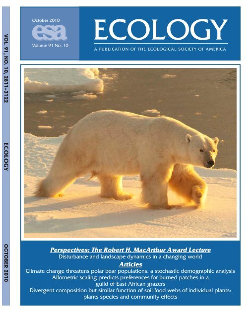
2884 CHRISTINE M. HUNTER ET AL.Ecology, Vol. 91, No. 10forecasts of the future environment. Although challenging,such assessments are necessary to forecast futuretrends and to inform policy debates and legal decisions.The U.S. Endangered Species Act, for example, requiresan assessment of extinction risks within the ‘‘foreseeablefuture’’ (16 U.S. Congress 1531, 1973).In this paper, we examine the current and projectedfuture effects of climate change on a population of polarbears (Ursus maritimus; see Plate 1). Our approach is todevelop stage-structured demographic models thatincorporate the observed responses of the stage-specificvital rates to sea ice conditions. We then present a novelapproach to connecting these demographic models toforecasts of future sea ice conditions from IPCC globalcirculation models (GCMs). The results reveal effects ofclimate on short-term transient dynamics, long-termpopulation growth rates (deterministic and stochastic)and environment-dependent stochastic growth in thenonstationary environment created by climate change.This study of climate effects was motivated by theneed for an evaluation of polar bear populationviability, following a petition to list the polar bear as athreatened species under the U.S. Endangered SpeciesAct (Center for Biological Diversity 2005). The Actrequires an evaluation of current conditions and aprediction of future risks to the population. Thisanalysis was a contribution to those goals. The finallisting decision concluded that declines in sea ice in polarbear habitat, both currently and in the future, pose athreat to the species, which is likely to becomeendangered in the foreseeable future. As a result, thepolar bear was listed as a threatened species in May 2008(U.S. Fish and Wildlife Service 2008).Polar bears and sea icePolar bears occur in most Arctic areas that are icecovered for much of the year. They depend on sea ice foraccess to their primary prey (ringed seals Phoca hispidaand bearded seals Erignathus barbatus) and for otheraspects of their life history (Stirling and Oritsland 1995,Stirling et al. 1999, Amstrup 2003). Polar bears preferhabitat on the continental shelf where they have greateraccess to prey. The retreat of sea ice beyond thecontinental shelf, and longer ice-free periods duringthe summer, are expected to reduce foraging success,increase nutritional stress, and increase the distancespolar bears must travel between seasonal use areas(Bergen et al. 2007). In some Arctic regions, the sea icemelts completely each year and polar bears are forced tospend the summer on shore. During this time they arelargely food deprived, relying on body fat accumulatedduring the previous year. Longer movements overrougher sea ice and more open water could also increasethe risks of injury or death (Monnett and Gleason2006), especially for cubs.Reductions in sea ice extent and/or duration havebeen associated with shifts toward more land-baseddenning, evidence of nutritional stress, reduced bodycondition, reproduction, survival, and body size forpolar bears in parts of their range (Stirling et al. 1999,Obbard et al. 2006, Stirling and Parkinson 2006,Fischbach et al. 2007, Regehr et al. 2007, Cherry et al.2008). In recent years in the southern Beaufort Sea therehave also been more numerous observations of unusualpredation attempts and of drowned, emaciated, andcannibalized polar bears (Amstrup et al. 2006, Monnettand Gleason 2006, Stirling et al. 2008).The study populationWe analyzed the population of polar bears in thesouthern Beaufort Sea, one of the 19 regions defined bythe IUCN Polar Bear Specialists Group (Aars et al.2006). This population has previously been studied byAmstrup et al. (1986, 2001, 2006) and Regehr et al.(2006). Population size in 2006 was estimated as 1526(95% confidence interval 1211–1841; Regehr et al. 2006).The study area (Fig. 1) lies on the northern coast ofAlaska and adjacent Canada, extending from Wainwright,Alaska in the west to Paulatuk, NorthwestTerritories, in the east (for details see Amstrup et al.1986, Regehr et al. 2009). A mark–recapture study ofthis population was conducted by the U.S. GeologicalSurvey and the Canadian Wildlife Service from 2001 to2006. During this period, polar bears were located usinghelicopters in the spring, and captured for marking oridentification. The data set consisted of 818 captures of627 tagged or radio-collared (approximately 6% ofcaptures) individuals. A detailed statistical analysis ofthese data using multistate mark–recapture methods(Regehr et al. 2009) provided estimates of the vital ratesused in our models.Demography and climate changeIn this study, we approach the demographic analysisof climate change effects using a sequence of models, ofincreasing sophistication, to explore different aspects ofthe problem (cf. Caswell 2001:644). We begin with adeterministic analysis of population growth in constantenvironments characterized by specific amounts of seaice. Then we construct a stochastic model with which weanalyze population growth in response to specifiedstatistical patterns of sea ice fluctuations. Finally, welink the stochastic models to forecasts of sea icefluctuations obtained from the output of a selected setof GCM climate models. This sequence of modelsproceeds from a constant environment, to a fluctuatingbut stationary environment, to a fluctuating andnonstationary environment.It is well known that demographic analysis caninfluence policy decisions. Policy, however, can alsodictate the direction of demographic analyses. In thecase of the Endangered Species Act, classification as athreatened species requires a finding that the species is atrisk of extinction ‘‘in the foreseeable future.’’ In the caseof the polar bear, the foreseeable future was interpretedby the U.S. Fish and Wildlife Service as 45 years from

October 2010 CLIMATE CHANGE AND POLAR BEARS2885FIG. 1. The southern Beaufort Sea study area, showing locations of polar bears captured from 2001 to 2006. The dashed line isthe population boundary, established by the International Union for the Conservation of Nature and Natural Resources (IUCN)Polar Bear Specialist Group. The white line is the 300-m bathymetry contour. The inset shows the four circumpolar ecoregionsdefined for polar bears by Amstrup et al. (2008). The figure is modified from Regehr et al. (2009).2007 (U.S. Fish and Wildlife Service 2007). Asymptoticanalyses using population growth rates, either stochasticor deterministic, may not properly address this question,so our analyses include transient projections with aparticular focus on 45 years, but also longer time periodsto 100 years. Comparisons of conclusions based onprojections of 45 years with those based on asymptoticpopulation growth rates may be instructive in futurelisting decisions.DEMOGRAPHIC MODEL STRUCTUREThe life cycleThe polar bear is the largest extant ursid. Survival isrelatively high; females as old as 32 years and males asold as 28 years have been reported (Stirling 1988).Females become pregnant for the first time in theirfourth or fifth year, and give birth for the first time intheir fifth or sixth year (Cronin et al. 2009). Femalesproduce litters of one to three cubs in a winter den.Dependent young remain with their mothers from birththrough the spring of their second year (Stirling 1988,Amstrup 2003), so the inter-birth interval for femalessuccessfully weaning young is at least 3 years.Our life cycle model included six stages, based on ageand reproductive status (Fig. 2). Stages 1, 2, and 3contain nonreproductive females aged 2, 3, and 4 years,respectively. Stage 4 comprises adult females available tobreed (i.e., without dependent young). Because mothersand cubs are not independent during the parental careperiod, we included these stages as mother–cub units;stage 5 comprises females accompanied by one or morecubs of the year, and stage 6 contains femalesaccompanied by one or more yearling cubs.This life cycle (Fig. 2) corresponds to a stagestructuredmatrix population model:nðt þ 1Þ ¼A t nðtÞð1Þwhere the vector n(t) gives the number of individuals ineach stage and the matrix A t projects the populationfrom t to t þ 1. The projection interval extends fromApril to April, to coincide with sampling, which occursin spring when females emerge from the den with theircubs. The entries in At are defined in terms of lower-levelvital rates: survival, r i (t); breeding, conditional onsurvival, b i (t); cub-of-the-year litter survival, r L0 (t);and yearling litter survival, r L1 . The survival probabilities,r i (t), are the probabilities of surviving from time t

2886 CHRISTINE M. HUNTER ET AL.Ecology, Vol. 91, No. 10FIG. 2. Polar bear life cycle graph; r i is the probability an individual in stage i survives from time t to t þ 1, r L0 and r L1 are theprobabilities that at least one member of a cub-of-the-year or yearling litter, respectively, survives from time t to t þ 1, f is theexpected size of a yearling litter that survives to 2 years, and b i is the conditional probability, given survival, of an individual instage i breeding and thereby producing a cub-of-the-year litter with at least one member surviving until the following spring.to t þ 1 of an individual in stage i. The breedingprobabilities are defined conditional on survival and arethe probability of breeding, given survival, of anindividual in stage i. Because we modeled stages 5 and6 as mother–cub units, transitions from these two stagesinclude litter survival probabilities. Litter survival is theprobability that at least one member of a cub-of-theyearlitter survives (r L0 ) or at least one member of ayearling litter survives (r L1 ).Fertility in this model appears on the arc from stage 6to stage 1. It depends on three quantities: survival of themother (r 6 ), survival of at least one member of ayearling litter (r L1 ), and the average number of 2-yearoldsin a surviving yearling litter ( f ). Details of thesecalculations are given in Appendix B. The sex ratio ofsurviving offspring is assumed to be 1:1.Demography and the sea ice environmentThe southern Beaufort Sea is covered with annual seaice from October through June, and partially orcompletely ice free from July through September whenthe sea ice retreats northward into the Arctic basin(Comiso 2006, Richter-Menge et al. 2006). To quantifysea ice availability to polar bears, Regehr et al. (2007,2009) developed an index, Ice(t), that measures theamount of time in year t during which polar bears areconfronted with a lack of ice in their preferred habitat.We defined Ice(t) as the number of days during year t inwhich the mean ice concentration was less than athreshold of 50%. Previous studies suggest that polarbears abandon sea ice below this threshold (Stirling et al.1999, Durner et al. 2004). Because polar bears stronglyprefer to forage over the continental shelf, Ice(t) wascalculated for waters on the continental shelf less than300m in depth (see Regehr et al. 2009 for details). Theindex Ice(t) has been referred to as ‘‘ice-free days’’(Regehr et al. 2007, 2009), and we will be consistent withthis, but a more accurate description might be ‘‘low-icedays.’’ Note, however that increases in ice(t) aredecreases in the amount of sea ice available to polarbears, and vice-versa.Parameter estimatesOur models are based on parameter estimatesobtained from a multistate mark–recapture analysis(Regehr et al. 2009). That analysis evaluated a set ofcandidate statistical models for the vital rates, based onthe life cycle structure. Those models were defined byconstraining some or all survival or breeding probabilitiesto be equal across stages, and by specifying possibleforms of temporal variation [time-invariant rates, timevaryingrates, and rates dependent on sea ice conditionsas measured by Ice(t)]. The results were model-averagedestimates (AIC-weighted) obtained using multi-modelinference (Burnham and Anderson 2002, Anderson2007). See Regehr et al. (2009) for a completedescription of the model sets and parameter estimationmethods. As is usual for mark–recapture estimation,survival probabilities estimated using these methodscannot distinguish true mortality from permanentemigration.Our parameter estimation procedure produced twomodel-averaged estimates to describe the effect of sea iceon polar bear vital rates. One set was obtained as anAIC-weighted average of all models, including thosewith parametric dependence of survival probabilities onthe covariate Ice(t). We refer to this as the parametricmodel set, and it is the most well-supported by the data.However, the results of any parametric model reflect, tosome degree, the choice of a parametric function, and itwould have been desirable to explore alternativefunctional forms. This was impossible because of the

October 2010 CLIMATE CHANGE AND POLAR BEARS2887short duration of the study. To examine the possibleeffects of the functional form used, we also analyzed aset of AIC-weighted estimates from which the modelswith parametric covariate dependence were excluded.We refer to this as the non-parametric model set.Comparison of projections from the parametric andnon-parametric model sets provides a check on theinfluence of the particular functional dependence onIce(t) (Regehr et al. 2009).We concluded that survival probabilities (r 1 –r 6 , andr L0 ) depended on both Ice(t) and time, while breedingprobabilities (b 4 , b 5 ) were time dependent, decreasing in2004 and 2005 (Regehr et al. 2009), when the number ofice-free days was particularly high (Table 1).Confidence intervals, standard errors, and samplingdistributions were obtained using a parametric bootstrapprocedure (details in Regehr et al. 2009). Togenerate a bootstrap sample, we first chose a model withprobability proportional to its AIC weight. A vector ofmark–recapture parameters was then drawn from amultivariate normal distribution with the estimatedmean and covariance matrix. This procedure wasrepeated for a specified number of times (usually10 000) to obtain the bootstrap sample set. The mark–recapture parameters were transformed as necessary,into demographic parameters, projection matrices,growth rates, and so on, as appropriate. Confidenceintervals were calculated using the percentile method.The bootstrap sample contains both model uncertainty(determined by the AIC weights associated with themodels) and parameter estimation uncertainty (determinedby the covariance matrix of the estimates).The only parameters not directly estimated from themark-recapture analysis were the survival of yearlinglitters (r L1 ) and fertility ( f ). Given an estimate of r L0from the mark–recapture estimation and an independentestimate of the frequency of one-cub and two-cub litters,it is possible to estimate individual cub survival andsubsequently yearling litter survival, individual yearlingsurvival, and the average number of two-year olds in asurviving yearling litter, f. Details of these calculationsare given in Appendix B.DETERMINISTIC DEMOGRAPHYDeterministic analysisWe used both the parametric and non-parametricmodel-averaged estimates to construct year-specificprojection matrices, A t , for each year, 2001–2005. Wecalculated the long-term population growth rate underthe conditions in year t as the dominant eigenvalue, k t ,of A t . The stable stage distribution and reproductivevalue distribution were calculated as the right and lefteigenvectors w and v, respectively, corresponding to k.Life table response experiment (LTRE) methods wereused to quantify the contributions of each of the vitalrates to the differences in population growth rate amongyears (Caswell 1989, 2001). To do so, we collected thevital rates (survival, litter survival, breeding) into aTABLE 1. Deterministic population growth rate k t , with 90%confidence intervals, standard error, proportion of bootstrapsamples ,1, and number of ice-free days [Ice(t)].Year (t) k t CILowerparameter vector h, and chose the year 2001 as areference condition. The difference in k between thereference year and year t is decomposed intok tk 2001 ’ X iUpperCIh ðtÞih ð2001Þ ]kið2Þ]h iwhere the sensitivity term is calculated at the mean ofthe vital rates for the reference year and year t. Eachterm in the summation is the contribution of one of thevital rates to the difference in k between the referenceyear and year t. A parameter may make a smallcontribution if it does not differ much among years orif k is not very sensitive to differences in that parameter.To examine transient effects, we projected populationgrowth for 45, 75, and 100 years, using Eq. 1 and aninitial population structure obtained from estimates ofthe southern Beaufort Sea population from 2004 to 2006(Regehr et al. 2006):n 0 ¼ð0:106 0:068 0:106 0:461 0:151 0:108 Þ > :ð3ÞDeterministic resultsEstimated population growth rates were greater than1 under the conditions experienced in 2001–2003 andless than 1 under the conditions experienced in 2004–2005 (Table 1). Confidence intervals were wide, but onlya small proportion of the bootstrap samples for yearswith more ice-free days (i.e., 2004 and 2005) projectedpositive population growth (for complete bootstrapdistributions, see Appendix C, Fig. C2).Including parametric dependence on sea ice makessurvival higher at low values of Ice, and lower at highvalues of Ice, compared to the nonparametric model setSEProportion, 1Ice(t)(days)Time-invariant modelall 0.997 0.755 1.053 0.105 0.57Parametric model set2001 1.059 0.083 1.093 0.269 0.24 902002 1.061 0.109 1.094 0.265 0.24 942003 1.036 0.476 1.107 0.207 0.41 1192004 0.765 0.541 0.932 0.120 1.00 1352005 0.799 0.577 0.959 0.122 0.99 134Nonparametric model set2001 1.017 0.810 1.088 0.092 0.43 902002 1.022 0.836 1.088 0.084 0.40 942003 1.075 0.903 1.129 0.077 0.19 1192004 0.801 0.549 1.000 0.135 0.95 1352005 0.895 0.446 1.020 0.185 0.88 134Notes: Results are shown for the parametric model set,including parametric dependence of vital rates on Ice(t), and forthe nonparametric model set, which permits time variation, butdoes not impose the parametric functional form.

2888 CHRISTINE M. HUNTER ET AL.Ecology, Vol. 91, No. 10Life table response experiment (LTRE) analysis forpopulation growth rate (k), measured relative to the year2001 for the nonparametric model set.TABLE 2.ParameterContribution to thedifference betweenk t and k 2001Proportionalcontribution2002 2003 2004 2005 2002 2003 2004 2005r 1 0.000 0.002 0.007 0.003 0.03 0.04 0.03 0.03r 2 0.000 0.002 0.007 0.003 0.03 0.04 0.03 0.03r 3 0.000 0.002 0.007 0.003 0.03 0.04 0.03 0.03r 4 0.001 0.008 0.091 0.045 0.25 0.15 0.42 0.36r 5 0.001 0.007 0.049 0.017 0.12 0.12 0.23 0.14r 6 0.000 0.004 0.018 0.008 0.09 0.07 0.08 0.06r L0 0.001 0.012 0.021 0.013 0.21 0.22 0.10 0.10b 4 0.001 0.011 0.006 0.025 0.15 0.19 0.03 0.20b 5 0.000 0.002 0.001 0.001 0.02 0.03 0.00 0.01f 0.000 0.006 0.003 0.002 0.06 0.10 0.01 0.02r L1 0.000 0.002 0.007 0.003 0.03 0.03 0.03 0.03Note: Values are expressed as contributions to the differencebetween k t and k 2001 and as a proportion of the total, where r iis the probability that an individual in stage i survives from timet to t þ 1, r L0 and r L1 are the probabilities that at least onemember of a cub-of-the-year or yearling litter, respectively,survives from time t to t þ 1, f is the expected size of a yearlinglitter that survives to 2 years, and b i is the conditionalprobability, given survival, of an individual in stage i breedingand thereby producing a cub-of-the-year litter with at least onemember surviving until the following spring.(Regehr et al. 2009). This amplifies the effect of reducedsea ice on survival, and carries over to the effect of Iceon population growth rates (Table 1). In our stochasticmodels, in which the severity of the impacts of reducedsea ice play a critical role, we will focus primarily on theresults from the nonparametric model set.The LTRE results (Table 2) show that the decline in kduring the low sea ice years (2004 and 2005) wasprimarily due to reduced survival of adult females (r 4 ,r 5 , and r 6 ), and secondarily to reduced breedingprobability (b 4 ). Thus, the estimated reductions insurvival and breeding in years with more ice-free daystranslated into dramatic reductions in populationgrowth rate.Fig. 3 shows k as a function of Ice(t), based on theAIC model-weighted parameter estimates, and the timespecifick t values from the nonparametric weightedmodel. The two agree well; population growth rate isrelatively insensitive to sea ice for Ice(t) , 127 days, butlonger ice-free seasons lead to a steep decline in k (Fig.3). Of course, extrapolation of the response of k beyondthe observed range depends entirely on the logisticparametric form assumed for the covariate dependence,and is unreliable. None of our analyses used suchextrapolation.Transient projections achieved exponential growthquickly, because the observed population vector (Eq. 3)is close to the stable stage distribution. Because thesemodels are linear, population size at time t in the futurerelative to initial population size can be interpreted interms of the proportional increase or decrease inpopulation size. To display the transient dynamics andtheir uncertainty, we use area plots (Fig. 4 and later).These plots show the proportion of simulations at anytime falling in a set of categories from drastic populationdecline (relative size , 0.001) to large increases (relativesize . 2). The proportion of simulations can beinterpreted as the probability of outcomes, over thespace defined by model uncertainty, parameter uncertainty,and, in our stochastic analyses, uncertainty aboutfuture environmental conditions.STOCHASTIC DEMOGRAPHYThe deterministic growth rate for a given yeardescribes the consequences of maintaining those conditionspermanently. To construct a stochastic model thataccounts for variation in conditions, we require astochastic model for the sea ice environment. To thisend, we classified sea ice conditions as ‘‘good’’ or‘‘poor,’’ depending on whether they would lead to avalue of k greater or less than one. This corresponds to athreshold value of Ice ’ 127 days. Consider anenvironment in which good and poor years occurindependently, with probability q of a poor year and 1q of a good year. In a poor year, the projection matrixis selected randomly from the matrices for 2004 and2005; in a good year, the projection matrix is selectedrandomly from the matrices for years 2001–2003. Thepopulation grows according to Eq. 1 with8A ð2001Þ with probability ð1 qÞ=3>< A ð2002Þ with probability ð1 qÞ=3A t ¼ A ð2003Þ with probability ð1 qÞ=3 ð4ÞA ð2004Þ with probability q=2>:A ð2005Þ with probability q=2:This algorithm treats the variability within the goodyears, and within the poor years, as crude estimates ofthe variation in the vital rates within these categoriesFIG. 3. Deterministic population growth rate, k, as afunction of the number of ice-free days, Ice(t). Diamonds aredeterministic population growth rates for 2001–2005 parameterestimates from the nonparametric model set.

October 2010 CLIMATE CHANGE AND POLAR BEARS2889FIG. 4. Uncertainty analysis of transient deterministic projections. The population is projected forward for 100 years using thevital rates estimated for the specified year in the parametric model set. Area plots show the proportion of 10 000 simulations inwhich the projected population size increased or declined to the specified fraction of the initial population. Simulations weresampled from the bootstrap distribution of parameter values.(see Caswell and Kaye 2001 for a similar approach in afire model).This stochastic model abstracts a continuous environmentalfactor into a finite set of discrete environmentalstates. Such models have been used frequently, asin studies of fire (Silva et al. 1991, Caswell and Kaye2001) and hurricanes (Pascarella and Horvitz 1998). Adiscrete environment model sacrifices some detail, but in

2890 CHRISTINE M. HUNTER ET AL.Ecology, Vol. 91, No. 10This critical frequency, about one poor ice year out ofsix, is exceeded by the frequency of poor ice yearsobserved between 1979 (when satellite imagery began)and 2005 (6/28 ¼ 0.21), by the frequency of poor yearsbetween 2001 and 2005 (2/5 ¼ 0.4), and by the frequencypredicted by IPCC climate models between now and theend of the century (Fig. 6).Uncertainty plots of stochastic transient projectionsare shown in Fig. 7. At the t ¼ 45 year time horizon, theprobability of a major decline (to less than 1% of currentsize) increases from 0.17 to 0.82 as the frequency of apoor ice year increases from q ¼ 0.1 to q ¼ 0.8. Thesituation at t ¼ 100 years is more dire; when q ¼ 0.1 theprobability of major decline is 0.24, increasing to 0.96when q ¼ 0.8.FIG. 5. The estimated stochastic growth rate, log k s ,asafunction of the frequency q of years with poor ice conditions:log k s . 0 indicates positive population growth; log k s , 0indicates negative population growth.our case it avoids errors that would result fromextrapolating the response of the vital rates to Icebeyond the observed range of Ice. Instead, ourconstruction assumes that conditions at any value ofIce . 127 days are no worse than those observed in2004–2005, and thus our model provides a lower boundon the effects of future climate change.Stochastic analysisThe stochastic population growth rate is1log k s ¼ limT!‘ T logjjA T 1 A 0 n 0 jj ð5Þwhere |||| is the 1-norm and n 0 is an arbitrary initialpopulation vector (e.g., Tuljapurkar 1990). We estimatedlog k s by Monte Carlo simulation with T ¼ 10 000. Toevaluate short-term transient population responses, wegenerated stochastic projections for 100 years, using theinitial population in Eq. 3. To evaluate the effects ofparameter uncertainty on stochastic growth, we repeatedthe calculations using models generated by samplingfrom the parametric bootstrap distribution of the vitalrates. Both the long-term growth rates and the shorttermprojections include sampling uncertainty, modeluncertainty, and environmental stochasticity.Stochastic resultsThe stochastic growth rate declines nearly linearly asthe frequency of poor years increases (Fig. 5). Thereexists a critical frequency of poor years (q ’ 0.165 forthe parametric model set; q ’ 0.17 for the nonparametricmodel set) above which log k s , 0 and the populationwill decline in the long run (Fig. 5). As expected, theresults from the parametric model set respond to sea iceconditions more strongly than those from the nonparametricmodel set.DEMOGRAPHIC PROJECTIONS UNDER CLIMATECHANGE FORECASTSModels and analysisThe stochastic model (Eq. 4) describes stochasticpopulation growth in a stationary environment characterizedby a specified frequency of poor ice years. TheArctic environment is not stationary, however, so wenow connect that model to forecasts of future sea iceconditions in response to climate change. Forecasts wereobtained from each of a set of 10 IPCC FourthAssessment Report (Solomon et al. 2007) fully coupledGCMs. The list of models is given in Appendix A: TableA1. The 10 GCMs were selected on the basis of theagreement of their 20th-century simulations with observedsea ice extent from 1953 to 1995 (see DeWeaver2007 for details). All GCM forecasts were based on the‘‘business as usual’’ greenhouse gas forcing scenario(SRES-A1B). Other forcing scenarios, some moreoptimistic and some more pessimistic, exist, but theA1B scenario is most appropriate for our purposesbecause it mimics recently observed emissions patternsand invokes neither societal changes that might increaseemission rates nor conscious mitigation efforts thatmight reduce them.Predictions of sea ice extent were obtained from theGCM output for an area including the southernBeaufort Sea and the surrounding divergent ice ecoregion(the Barents, Beaufort, Chukchi, Kara, andLaptev Seas; see Amstrup et al. 2008, Rigor and Wallace2004). Sea ice trends in recent decades have followed asimilar pattern throughout this region (Stroeve et al.2007), justifying our application to the southernBeaufort Sea.Obtaining forecasts of the frequency of poor ice yearsfrom the GCM output proceeded in three steps. First,we calculated Ice(t) from the output, obtaining thenumber of ‘‘ice-free’’ months in each year from 2005 to2100. These were transformed to ice-free days bymultiplying by 30. To standardize the starting points,we additively adjusted the output of each GCM so thatIce(2005) ¼ 114.4 days, the mean of Ice(t) during 2000–

October 2010 CLIMATE CHANGE AND POLAR BEARS2891FIG. 6. (a) Frequency of poor ice conditions from 1979 to 2006, smoothed with a Gaussian kernel smoother with standarddeviation u ¼ 1.5, 2, and 3 (see Copas 1983). Data are from Fig. 3 in Regehr et al. (2007). (b) The projected probability of a poor iceyear, from 2005 to 2100, from 10 general circulation model (GCM) climate models. Kernel standard deviation ¼ 2.5.2005. Second, we transformed the value of Ice(t) toabinary environmental state, classifying year t as good ifIce(t) . 127 days, or poor if Ice(t) , 127 days. The thirdstep was to extract trends in the frequency of poor yearsfrom the sequence of binary outcomes. Such calculationsalways require some smoothing; we applied a Gaussiankernel smoother as described by Copas (1983; see Smithet al. 2005 for an ecological application similar to thisone). The kernel standard deviation (2.5 years) waschosen, as suggested by Copas (1983), as a subjectivecompromise between smoothing and variation.Each of the 10 GCMs thus produced a time series offorecast values of q(t) from 2005 to 2100. We used thesefrequencies to project the polar bear population, withn(0) given by Eq. 3 and A t chosen randomly at each timestep with probabilities given by Eq. 4 and the forecastvalue of q(t). To evaluate the effects of uncertainty, werepeated the calculations with each GCM using 1000

2892 CHRISTINE M. HUNTER ET AL.Ecology, Vol. 91, No. 10FIG. 7. Uncertainty analysis of transient stochastic projections. Area plots show the proportion of 10 000 simulations in whichprojected population size increased or declined to the specified fraction of the initial population, given the probability q of a poorice year and vital rates from the parametric model set. Simulations were sampled from the bootstrap distribution of parametervalues.bootstrapped parameter estimates, for a total of 10 000calculations. The resulting variability includes uncertaintydue to statistical models, parameter estimation,and variation among the GCMs.Climate projection resultsThe estimates of q(t) from the output of the 10 GCMsdiffer in detail, but all predict an increase in thefrequency of poor Ice years over the next century (Fig.6). The frequency of such years reaches 1 by the year2100 (indeed, this level is reached by all but one of theclimate models by the year 2055). Because the environmentforecast by the GCMs is not stationary (both themean and the variance change over time), it is impossibleto calculate asymptotic stochastic growth rates from thismodel. Transient projections, however, are shown inFig. 8, for both model sets. The projections by the year2100 are overwhelmingly negative; the probability of adecline of 50% or more is 0.92 (nonparametric modelset) or 0.99 (parametric model set). The probability ofdecline of 99% or more is 0.80 (nonparametric) or 0.94(parametric). There is some probability of short-termincrease, over the next 20–40 years, generated largely bythe differences among climate models in how soon thefrequency of poor ice years begins to increase (Fig. 6).Since that frequency has, in fact, already been increasingsince 1980 (Fig. 6), these short-term increases areunlikely to be realized.DISCUSSIONLinking climate models and demographyThe effect of climate change on population growthand viability is a pressing ecological problem. At themost basic level it proceeds by measuring the effect of

October 2010 CLIMATE CHANGE AND POLAR BEARS2893climate-related variables (e.g., temperature) on anecological process (e.g., survival). If the process isrelated to population growth and the direction ofenvironmental change can be predicted, then a qualitativeprediction of the effect of climate change can beobtained.To go beyond such a qualitative prediction requiresinformation on the sensitivity of the entire life cycle (oras much of it as possible) to the environment, and aquantitative prediction of future environmental changes.In this paper, we obtained such a quantitative predictionby a novel approach to linking environment-dependentdemographic models to the output of GCMs. Thisapproach, which is applicable to other species, has threesteps. First, a life cycle model was parameterized as afunction of the environment, in this case, an index of seaice extent. Second, a stochastic demographic model wasdeveloped to compute population growth as a functionof environmental conditions and their fluctuations.Third, a forecast of environmental changes was extractedfrom GCM output. In our case, that forecast consistsof a time series of the frequency of poor ice conditions.This approach can be applied to other species andsituations (e.g., Jenouvrier et al. 2009). The discretizationof the environmental states, as we did here, avoidsthe need to extrapolate continuous relationships betweenthe environment and the vital rates beyond therange of observed conditions. This makes our predictionsof polar bear responses conservative, because nomatter how large Ice(t) becomes, the vital rates in themodel will be no worse than those observed during thepoor ice years of the study. However, given sufficientlydetailed information on both climate and the responseof vital rates, the analysis could use a continuousenvironment model (see Jenouvrier et al. 2009 for acomparison of discrete and continuous approaches).UncertaintiesManagement decisions must often be made in the faceof uncertainty, because information is limited andenvironments are variable. Therefore, where possible,analyses of climate effects should quantify the uncertaintyof the results on which management decisions arebased. This was particularly important in the listingdecision for the polar bear, and our analyses purposelyincluded several different kinds of uncertainty.Burnham and Anderson (2002) and Anderson (2007)have emphasized the importance of including modelselection uncertainty along with estimation uncertainty.Our parametric bootstrap distributions include bothtypes of uncertainty. We also recognize the uncertaintyinvolved in parametric specification of the ice-dependenceof the vital rates, and therefore analyzed bothnonparametric and parametric model sets. Althoughprojections based on the nonparametric model set,excluding parametric ice dependence, are conservativein the sense of yielding a weaker response to sea iceconditions, it is important to remember that theFIG. 8. Stochastic simulations of population growth underconditions predicted by 10 IPCC climate models. Area plotsshow the proportion of 10 000 simulations in which projectedpopulation size after t years increased or declined to a specifiedfraction of initial population size for (a) the parametric modelset and (b) the nonparametric model set. Simulations wereobtained as samples of 1000 from the bootstrap distribution ofparameter values, for each climate model.parametric model set is the one most well-supportedby the data. Both analyses lead to the same conclusions(Fig. 3).In addition, we used a series of deterministic andstochastic population models to assess potential populationresponse to changing ice conditions. The consistencyof results across this series of models strengthensour inference. Such a sequence is the only way toquantitatively assess the effects of different types ofuncertainty in assessment of population status andresponse to environmental conditions.Two aspects of the estimation procedures are worthdiscussing because they might have artificially reducedsurvival probabilities. One is harvest, which is not

2894 CHRISTINE M. HUNTER ET AL.Ecology, Vol. 91, No. 10PLATE 1. A subadult polar bear contemplates how to negotiate an area of melting sea ice. Polar bears are classified as marinemammals, but they are not aquatic. They feed upon ringed and bearded seals and other aquatic mammals that they catch from thesea-ice surface. They travel mainly by walking on the sea ice rather than swimming. Rising global temperatures mean that polarbears increasingly are exposed to marginal ice or open water where historically there were stable sea-ice habitats. The futurepopulation impacts of more prolonged periods, during which suitable sea ice is unavailable, are projected to be severe. Photo Ó2009 Daniel J. Cox/hNaturalExposures.comi.incorporated in our projections. Polar bears in thesouthern Beaufort Sea are subject to regulated hunts bynative user groups in the United States and Canada(Brower et al. 2002). Hunters are discouraged fromtaking females with dependent cubs but subadultfemales and adult females without cubs are currentlysubject to harvest at a rate of ’0.019 (Regehr et al.2007). Although the impact of this harvest is included inthe survival estimates for these stages; this level ofharvest has a negligible effect on population growth rate(Hunter et al. 2007).The second issue is emigration. Nonrandom temporaryemigration can lead to survival estimates that arenegatively biased at the end of a study. However, Regehret al. (2009) investigated this, and found no evidence ofnon-random temporary emigration. Although the powerof the analysis was limited due to the short studyduration, available data indicated that temporaryemigration did not create an important bias of survivalrates used in this study. Permanent emigration cannot bedistinguished from mortality. However, radio telemetrystudies, which began in the Beaufort Sea in 1981, haveconfirmed that polar bears maintain a high degree offidelity to this geographic region. Although individualanimal utilization distributions are very large andvariable, over multi-year periods they do constitute‘‘home ranges’’ (Amstrup et al. 2000). The permanentmigration of collared animals beyond the Beaufort Searegion has been so rare that the description of themovement of the one bear that did permanentlyemigrate was deemed worthy of publication (Durnerand Amstrup 1995).Polar bear population statusSummer sea ice in the Arctic is expected to continue todecline (e.g., IPCC 2007, Overland and Wang 2007,Stroeve et al. 2007). Our analyses demonstrate that thisdecline poses a serious threat to the continued persistenceof the southern Beaufort Sea population of polarbears. The current southern Beaufort Sea populationnumbers about 1500 individuals (Regehr et al. 2006), soa decline to 1% of current size would almost certainlyimply extinction. The probability of this outcome isestimated at 0.80–0.94 by the year 2100, which iscertainly a serious risk.The ice-free period in the southern Beaufort Seaincreased by approximately 50% between 2001–2003 and2004–2005. At the same time, survival and breedingprobabilities declined (Regehr et al. 2007). The vitalrates estimated in years with low values of Ice(t) led topositive population growth, but when Ice(t) exceedsabout 127 days, the population growth rate becomesnegative due to reductions in adult survival and breedingprobabilities. Asymptotic and short-term transientprojections showed the same results.Our stochastic analysis found that a frequency of poorice years greater than q ’ 0.17 produces a negativestochastic growth rate. This critical frequency is less

October 2010 CLIMATE CHANGE AND POLAR BEARS2895than the observed frequency of poor years from 1979 to2005, the available record from satellite imagery. Theobserved frequency of poor ice years, q ¼ 0.2, from 1979to 2005 (the available satellite record) exceeds thisthreshold, and would lead to a stochastic growth rate oflog k s ¼ 0.012 (parametric model) or 0.006 (nonparametricmodel).Arctic sea ice extent at the end of the summer of 2005was the lowest ever observed. This record was broken in2007, and approached in 2008. If thinning multiyear ice,more extensive open water and albedo effects createpositive feedback loops leading to further reductions(Maslanik et al. 2007), the fate of polar bears in otherlocations, even where populations have been stable (e.g.,the northern Beaufort Sea) will also be in doubt. Recentshipboard surveys in the southern Beaufort Sea (Barberet al. 2009) found summer sea ice there to be eventhinner and more broken than shown in satellite images.Comparisons of these growth rates estimated herewith trajectories of population size are hampered by thelack of reliable population size estimates. The claim,commonly repeated in the press, that worldwide polarbear populations have increased fourfold since the 1960shas no basis in the scientific literature (Dykstra 2008).Some increases in polar bear populations occurred in the1970s as harvesting was reduced, but there is no evidencethat these increases continued, and such recoveries,where they occurred, are irrelevant to the effects ofrecent changes in the availability of sea ice. In thesouthern Beaufort Sea, Amstrup et al. (1986) reported acrude estimate of population size of N ’ 1800 bears inthe mid-1980s. Regehr et al. (2006) estimated N ’ 1500bears in 2006. Amstrup et al. (2001) suggested thepopulation may have remained constant or evenincreased between the 1980s and the late 1990s.However, if the difference between 1800 bears and1500 bears represents a real decline, and if that declineoccurred over 15 years, it would represent an averageannual growth rate of 0.012. Over 20 years, such adecline would imply an average annual growth rate of0.009. This further suggests that our estimates ofstochastic growth rate are reasonable. This comparisonwith our calculated growth rate is very rough, because ofthe different sources of historical data and the highdegree of uncertainty around these population estimates.Nevertheless, the comparison supports the modelresults.The mechanisms linking sea ice to survival andreproduction of polar bears are not known in detail.Reduced prey availability no doubt plays a role (Stirlingand Smith 2004), because polar bears are dependentupon sea ice for capturing prey (Amstrup 2003) andtheir preferred foraging area is the water over thecontinental shelf. In addition, reduced sea ice extent mayforce polar bears to swim longer distances, increasingtheir risk of drowning or starvation (Monnett andGleason 2006). The thinner ice that reforms after largesummer ice retreats also may be less suitable for polarbear foraging (Stirling et al. 2008). Reduced sea ice willundoubtedly also affect other ice-dependent species (see,e.g., Gaston et al. 2005) and many food web links maybe involved in these effects (Huntington and Moore2008, Moline et al. 2008).We have shown that global warming is likely to haveprofoundly negative effects on future growth rates ofpolar bear populations. A warmer world will have lesssea ice and hence less polar bear habitat. Geographicalvariation in the nature of sea ice and in predictions ofthe retreat of sea ice habitat (Durner et al. 2009) suggeststhat polar bears in different parts of their current rangewill be affected at different rates. Nonetheless, ouranalyses, which incorporated sea ice and other uncertainties,projected that by mid century, the effects ofglobal warming on polar bears will be severe. If currentGCM outcomes are correct, there is a high probabilitythat the Beaufort Sea population of polar bears willdisappear by the end of the century. Because all polarbears are dependent on sea ice for securing their prey, itis reasonable to expect that the effects of global warmingon polar bears of the southern Beaufort Sea willultimately extend to polar bears throughout their range.This and other related findings provided the primarymotivation for listing polar bears, in May of 2008, as athreatened species under the U.S. Endangered SpeciesAct (U.S. Fish and Wildlife Service 2008).ACKNOWLEDGMENTSWe acknowledge primary funding for model developmentand analysis from the U.S. Geological Survey and additionalfunding from the National Science Foundation (DEB-0343820and DEB-0816514), NOAA, the Ocean Life Institute and theArctic Research Initiative at WHOI, and the Institute of ArcticBiology at the University of Alaska–Fairbanks. Funding for thecapture–recapture effort in 2001–2006 was provided by the U.S.Geological Survey, the Canadian Wildlife Service, the Departmentof Environment and Natural Resources of the Governmentof the Northwest Territories, and the Polar ContinentalShelf Project, Ottawa, Canada. We thank G. S. York, K. S.Simac, M. Lockhart, C. Kirk, K. Knott, E. Richardson, A. E.Derocher, and D. Andriashek for assistance in the field. D.Douglas and G. Durner assisted with analyses of radiotelemetryand remote sensing sea ice data. We thank J. Nichols, M.Udevitz, E. Cooch, and J.-D. Lebreton for helpful commentsand discussions.LITERATURE CITEDAars, J., N. J. Lunn, and A. E. Derocher. 2006. Polar bears:proceedings of the 14th working meeting of the IUCN/SSCpolar bear specialists group. International Union forConservation of Nature and Natural Resources, Gland,Switzerland and Cambridge, UK.Amstrup, S. C. 2003. Polar bear, Ursus maritimus. Pages 587–610 in G. A. Feldhamer, B. C. Thompson, and J. A.Chapman, editors. Mammals of North America: biology,management, and conservation. Johns Hopkins UniversityPress, Baltimore, Maryland, USA.Amstrup, S. C., G. Durner, I. Stirling, N. J. Lunn, and F.Messier. 2000. Movements and distribution of polar bears inthe Beaufort Sea. Canadian Journal of Zoology 78:948–966.Amstrup, S. C., B. G. Marcot, and D. C. Douglas. 2008. ABayesian network modeling approach to forecasting the 21stcentury worldwide status of polar bears. Pages 213–268 inE. T. DeWeaver, C. M. Bitz, and L.-B. Tremblay, editors.

2896 CHRISTINE M. HUNTER ET AL.Ecology, Vol. 91, No. 10Arctic sea ice decline: observations, projections, mechanisms,and implications. Geophysics monograph series 180. AGU,Washington, D.C., USA.Amstrup, S. C., T. L. McDonald, and I. Stirling. 2001. Polarbears in the Beaufort Sea: a 30 year mark–recapture casehistory. Journal of Agricultural, Biological, and EnvironmentalStatistics 6:221–234.Amstrup, S. C., I. Stirling, and J. W. Lentfer. 1986. Past andpresent status of polar bears in Alaska. Wildlife SocietyBulletin 14:241–254.Amstrup, S. C., I. Stirling, T. S. Smith, C. Perham, and G. W.Thiemann. 2006. Recent observations of intraspecific predationand cannibalism among polar bears in the southernBeaufort Sea. Polar Biology 29:997–1002.Anderson, D. R. 2007. Model-based inference in the lifesciences: a primer on evidence. Springer-Verlag, New York,New York, USA.Barber, D. G., R. Galley, M. G. Asplin, R. De Abreu, K.Warner, M. Pucko, M. Gupta, S. Prinsenberg, and S. Julien.2009. The perennial pack ice in the southern Beaufort Seawas not as it appeared in the summer of 2009. GeophysicalResearch Letters 36:L24501.Bergen, S., G. M. Durner, D. C. Douglas, and S. C. Amstrup.2007. Predicting movements of female polar bears betweensummer sea ice foraging habitats and terrestrial denninghabitats of Alaska in the 21st century: proposed methodologyand pilot assessment. Administrative Report. USGSAlaska Science Center, Anchorage, Alaska, USA.Boyd, I., S. Wanless, and C. J. Camphuysen. 2006. Toppredators in marine ecosystems: their role in monitoring andmanagement. Cambridge University Press, Cambridge, UK.Brower, C. D., A. Carpenter, M. L. Branigan, W. Calvert, T.Evans, A. S. Fischbach, J. A. Nagy, S. Schliebe, and I.Stirling. 2002. The polar bear management agreement for thesouthern Beaufort Sea: An evaluation of the first ten years ofa unique conservation agreement. Arctic 55:362–372.Burnham, K. P., and D. R. Anderson. 2002. Model selectionand multimodel inference: a practical information-theoreticapproach. Second edition. Springer-Verlag, New York, NewYork, USA.Caswell, H. 1989. The analysis of life table responseexperiments. I. Decomposition of effects on populationgrowth rate. Ecological Modelling 46:221–237.Caswell, H. 2001. Matrix population models. Second edition.Sinauer, Sunderland, Massachusetts, USA.Caswell, H., and T. Kaye. 2001. Stochastic demography andconservation of an endangered plant (Lomatium bradshawii)in a dynamic fire regime. Advances in Ecological Research32:1–51.Center for Biological Diversity. 2005. Petition to list the polarbear (Ursus maritimus) as a threatened species under theEndangered Species Act. Before the Secretary of the Interior2-16-2005. hhttp://www.biologicaldiversity.org/species/mammals/polar_bear/pdfs/15976_7338.pdfiCherry, S. G., A. E. Derocher, I. Stirling, and E. Richardson.2008. Fasting physiology of polar bears in relation toenvironmental change and breeding behavior in the BeaufortSea. Polar Biology 32:383–391.Comiso, J. C. 2006. Arctic warming signals from satelliteobservations. Weather 61:70–76.Convey, P., and R. I. L. Smith. 2006. Responses of terrestrialAntarctic ecosystems to climate change. Plant Ecology 182:1–10.Copas, J. B. 1983. Plotting p against x. Applied Statistics 32:25–31.Cronin, M. A., S. C. Amstrup, S. L. Talbot, G. K. Sage, andK. S. Amstrup. 2009. Genetic variation, relatedness, andeffective population size of polar bears (Ursus maritimus) inthe southern Beaufort Sea, Alaska. Journal of Heredity 100:681–690.DeWeaver, E. 2007. Uncertainty in climate model projectionsof Arctic sea ice decline: an evaluation relevant to polarbears. Administrative Report. USGS Alaska Science Center,Anchorage, Alaska, USA.Durner, G. M., and S. C. Amstrup. 1995. Movements of a polarbear from northern Alaska to northern Greenland. Arctic 48:338–341.Durner, G. M., S. C. Amstrup, R. M. Nielson, and T. L.McDonald. 2004. The use of sea ice habitat by female polarbears in the Beaufort Sea. Report to Minerals ManagementService for OCS Study 2004–14. U.S. Geological Survey,Alaska Science Center, Anchorage, Alaska, USA.Durner, G. M., et al. 2009. Predicting 21st century polar bearhabitat distribution from global climate models. EcologicalMonographs 79:25–58.Dykstra, P. 2008. Magic number: a sketchy fact about polarbears keeps going . . . and going . . . and going. Society ofEnvironmental Journalists, online article 15, Summer 2008.hhttp://www.sej.org/publications/alaska-and-hawaii/magicnumber-a-sketchy-fact-about-polar-bears-keeps-goingandgoing-aniFischbach, A. S., S. C. Amstrup, and D. C. Douglas. 2007.Landward and eastward shift of Alaskan polar bear denningassociated with recent sea ice changes. Polar Biology 30:1395–1405.Gaston, A. J., H. G. Gilchrist, and M. L. Mallory. 2005.Variation in ice conditions has strong effects on the breedingof marine birds at Prince Leopold Island, Nunavut.Ecography 28:331–344.Grosbois, V., O. Gimenez, J.-M. Gaillard, R. Pradel, C.Barbraud, J. Clobert, A. P. Moller, and H. Weimerskirch.2008. Assessing the impact of climate variation on survival invertebrate populations. Biological Reviews 83:357–399.Hunter, C. M., H. Caswell, M. C. Runge, E. V. Regehr, S. C.Amstrup, and I. Stirling. 2007. Polar bears in the SouthernBeaufort Sea II: demography and population growth inrelation to sea ice conditions. Administrative Report. USGSAlaska Science Center, Anchorage, Alaska, USA.Huntington, H. P., and S. E. Moore. 2008. Arctic marinemammals and climate change. Ecological Applications18(Supplement):S1–S2.IPCC 2007. Summary for policymakers. Pages 1–18 in S.Solomon, D. Qin, M. Manning, Z. Chen, M. Marquis, K. B.Averyt, M. Tignor, and H. L. Miller, editors. Climate change2007: the physical science basis. Contribution of WorkingGroup I to the Fourth Assessment Report of the IntergovernmentalPanel on Climate Change. Cambridge UniversityPress, New York, New York, USA.Jenouvrier, S., H. Caswell, C. Barbraud, and H. Weimerskirch.2009. Demographic models and IPCC climate projectionspredict the decline of an emperor penguin population.Proceedings of the National Academy of Sciences USA106:1844–1847.Keith, D. A., H. R. Akcakaya, W. Thuiller, G. F. Midgley,R. G. Pearson, S. J. Phillips, H. M. Regan, M. B. Araujo,and T. G. Rebelo. 2008. Predicting extinction risks underclimate change: coupling stochastic population models withdynamic bioclimatic habitat models. Biology Letters 4:560–563.Laidre, K. L., I. Stirling, L. F. Lowry, O. Wiig, M. P. Heide-Jorgensen, and S. H. Ferguson. 2008. Quantifying thesensitivity of arctic marine mammals to climate-inducedhabitat change. Ecological Applications (Supplement)18:S97–S125.Maslanik, J. A., C. Fowler, J. Stroeve, S. Drobot, J. Zwally, D.Yi, and W. Emery. 2007. A younger, thinner Arctic ice cover:Increased potential for rapid, extensive sea-ice loss. GeophysicalResearch Letters 34GL032043.Moline, M. A., N. J. Karnovsky, Z. Brown, G. J. Divoky, T. K.Frazer, C. A. Jacoby, J. J. Torres, and W. R. Fraser. 2008.High latitude changes in ice dynamics and their impact onpolar marine ecosystems. Annals of the New York Academyof Sciences 1134:267–319.

October 2010 CLIMATE CHANGE AND POLAR BEARS2897Monnett, C., and J. S. Gleason. 2006. Observations of mortalityassociated with extended open-water swimming by polarbears in the Alaskan Beaufort Sea. Polar Biology 29:681–687.Obbard, M. E., M. R. L. Cattet, T. Moody, L. Walton, D.Potter, J. Inglis, and C. Chenier. 2006. Temporal trends in thebody condition of southern Hudson Bay polar bears. ClimateChange Research Information Note, No. 3. Applied Researchand Development Branch, Ontario Ministry ofNatural Resources, Sault Sainte Marie, Ontario, Canada.Overland, J. E., and M. Wang. 2007. Future regional Arctic seaice declines. Geophysical Research Letters 34GL030808.Parmesan, C. 2006. Ecological and evolutionary responses torecent climate change. Annual Review of Ecology Evolutionand Systematics 37:637–669.Pascarella, J. B., and C. C. Horvitz. 1998. Hurricanedisturbance and the population dynamics of a tropicalunderstory shrub: megamatrix elasticity analysis. Ecology79:547–563.Perovich, D. K., and J. A. Richter-Menge. 2009. Loss of sea icein the Arctic. Annual Review of Marine Science 1:417–441.Regehr, E. V., S. C. Amstrup, and I. Stirling. 2006. Polar bearpopulation status in the southern Beaufort Sea. Open-FileReport 2006-1337. U.S. Geological Survey, Reston, Virginia,USA.Regehr, E. V., C. M. Hunter, H. Caswell, S. C. Amstrup, and I.Stirling. 2009. Survival and breeding of polar bears in thesouthern Beaufort Sea in relation to sea ice. Journal ofAnimal Ecology 79:117–127.Regehr, E. V., C. M. Hunter, H. Caswell, I. Stirling, and S. C.Amstrup. 2007. Polar bears in the southern Beaufort Sea I:Survival and breeding in relation to sea ice conditions, 2001–2006. Administrative Report. USGS Alaska Science Center,Anchorage, Alaska, USA.Richter-Menge, J., et al. 2006. State of the Arctic report. Specialreport. NOAA/OAR/PMEL, Seattle, Washington, USA.Rigor, I. G., and J. M. Wallace. 2004. Variations in the age ofArctic sea-ice and summer sea-ice extent. GeophysicalResearch Letters 31GL019492.Rode, K. D., S. C. Amstrup, and E. V. Regehr. 2010. Reducedbody size and cub recruitment in polar bears associated withsea ice decline. Ecological Applications 20:768–782.Serreze, M. C., and J. A. Francis. 2006. The arctic amplificationdebate. Climate Change 76:241–264.Silva, J. F., J. Raventos, H. Caswell, and M. C. Trevisan. 1991.Population responses to fire in a tropical savanna grassAndropogon semiberbis: a matrix model approach. Journal ofEcology 79:345–356.Smith, M., H. Caswell, and P. Mettler-Cherry. 2005. Stochasticflood and precipitation regimes and the population dynamicsof a threatened floodplain plant. Ecological Applications 15:1036–1052.Solomon, S., D. Qin, M. Manning, Z. Chen, M. Marquis, K. B.Averyt, M. Tignor, and H. L. Miller, editors. 2007. Climatechange 2007: the physical science basis. Contribution ofWorking Group I to the Fourth Assessment Report of theIntergovernmental Panel on Climate Change. CambridgeUniversity Press, Cambridge, UK.Stirling, I. 1988. Polar bears. University of Michigan Press, AnnArbor, Michigan, USA.Stirling, I., N. J. Lunn, and J. Iacozza. 1999. Long-term trendsin the population ecology of polar bears in western HudsonBay in relation to climatic change. Arctic 52:294–306.Stirling, I., and N. A. Oritsland. 1995. Relationships betweenestimates of ringed seal and polar bear populations in theCanadian Arctic. Canadian Journal of Fisheries and AquaticSciences 52:2594–2612.Stirling, I., and C. L. Parkinson. 2006. Possible effects ofclimate warming on selected populations of polar bears(Ursus maritimus) in the Canadian Arctic. Arctic 59:261–275.Stirling, I., E. Richardson, G. W. Thiemann, and A. E.Derocher. 2008. Unusual predation attempts of polar bearson ringed seals in the southern Beaufort Sea: possiblesignificance of changing spring ice conditions. Arctic 60:14–22.Stirling, I., and T. G. Smith. 2004. Implications of warmtemperatures, and an unusual rain event for the survival ofringed seals on the coast of southeastern Baffin Island. Arctic57:59–67.Stroeve, J. C., M. M. Holland, W. Meier, T. Scambos, and M.Serreze. 2007. Arctic sea ice decline: faster than forecast.Geophysical Research Letters 34GL029703.Tuljapurkar, S. 1990. Population dynamics in variable environments.Springer-Verlag, New York, New York, USA.U.S. Fish and Wildlife Service. 2007. Endangered andthreatened wildlife and plants: 12-month petition findingand proposed rule to list the polar bear (Ursus maritimus) asthreatened throughout its range. Federal Register 72(5):1064–1099.U.S. Fish and Wildlife Service. 2008. Endangered andthreatened wildlife and plants: determination of threatenedstatus for the polar bear (Ursus maritimus) throughout itsrange. Final Rule. Federal Register 73:28211–28303.Walsh, J. E. 2008. Climate of the Arctic marine environment.Ecological Applications 18(Supplement):S3–S22.APPENDIX AProjection matrices (Ecological Archives E091-204-A1).APPENDIX BCalculation of fertility (Ecological Archives E091-204-A2).APPENDIX CIPCC models and bootstrap sampling results (Ecological Archives E091-204-A3).