Lyapunov exponents of the predator prey model Ljapunovovy ...

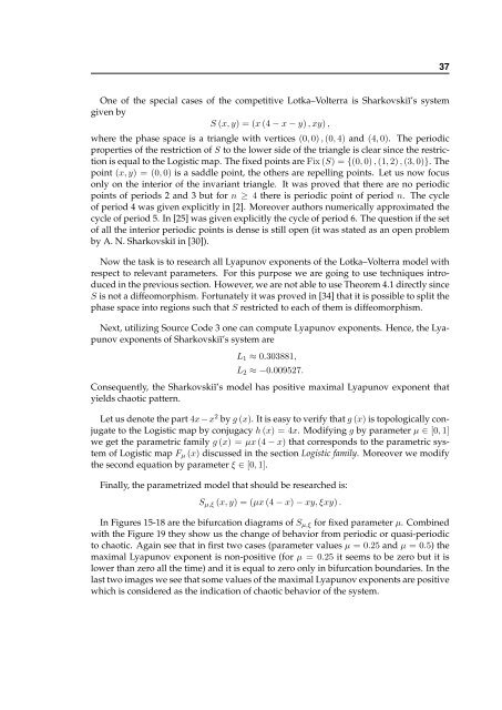
37One of the special cases of the competitive Lotka–Volterra is Sharkovskiĭ’s systemgiven byS (x, y) = (x (4 − x − y) , xy) ,where the phase space is a triangle with vertices (0, 0) , (0, 4) and (4, 0). The periodicproperties of the restriction of S to the lower side of the triangle is clear since the restrictionis equal to the Logistic map. The fixed points are Fix (S) = {(0, 0) , (1, 2) , (3, 0)}. Thepoint (x, y) = (0, 0) is a saddle point, the others are repelling points. Let us now focusonly on the interior of the invariant triangle. It was proved that there are no periodicpoints of periods 2 and 3 but for n ≥ 4 there is periodic point of period n. The cycleof period 4 was given explicitly in [2]. Moreover authors numerically approximated thecycle of period 5. In [25] was given explicitly the cycle of period 6. The question if the setof all the interior periodic points is dense is still open (it was stated as an open problemby A. N. Sharkovskiĭ in [30]).Now the task is to research all Lyapunov exponents of the Lotka–Volterra model withrespect to relevant parameters. For this purpose we are going to use techniques introducedin the previous section. However, we are not able to use Theorem 4.1 directly sinceS is not a diffeomorphism. Fortunately it was proved in [34] that it is possible to split thephase space into regions such that S restricted to each of them is diffeomorphism.Next, utilizing Source Code 3 one can compute Lyapunov exponents. Hence, the Lyapunovexponents of Sharkovskiĭ’s system areL 1 ≈ 0.303881,L 2 ≈ −0.009527.Consequently, the Sharkovskiĭ’s model has positive maximal Lyapunov exponent thatyields chaotic pattern.Let us denote the part 4x−x 2 by g (x). It is easy to verify that g (x) is topologically conjugateto the Logistic map by conjugacy h (x) = 4x. Modifying g by parameter µ ∈ [0, 1]we get the parametric family g (x) = µx (4 − x) that corresponds to the parametric systemof Logistic map F µ (x) discussed in the section Logistic family. Moreover we modifythe second equation by parameter ξ ∈ [0, 1].Finally, the parametrized model that should be researched is:S µ,ξ (x, y) = (µx (4 − x) − xy, ξxy) .In Figures 15-18 are the bifurcation diagrams of S µ,ξ for fixed parameter µ. Combinedwith the Figure 19 they show us the change of behavior from periodic or quasi-periodicto chaotic. Again see that in first two cases (parameter values µ = 0.25 and µ = 0.5) themaximal Lyapunov exponent is non-positive (for µ = 0.25 it seems to be zero but it islower than zero all the time) and it is equal to zero only in bifurcation boundaries. In thelast two images we see that some values of the maximal Lyapunov exponents are positivewhich is considered as the indication of chaotic behavior of the system.