Microeconomics Cue Card - the Educator Login page!

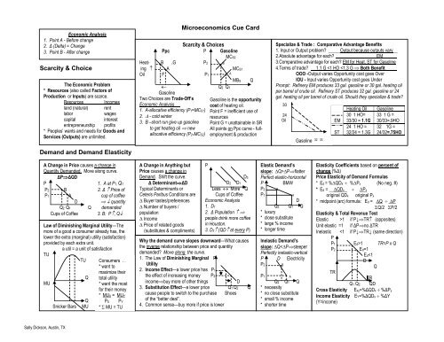
Supply & Supply ElasticityA Change in Price causes a change in QuantitySupplied. Move along curve.ΔPΔQSEco AnalysisP S 1. A at P1, QS1P2 B 2. Δ Price ofP1 A cup of coffee QuantityQ1 Q2 Q suppliedCups of Coffee3. B: P2, QS2A Change in Anything butPrice causes a change inSupply. Shift the curve.Δ DeterminantΔSTypical Determinants orCeteris Paribus conditions resource (factor) prices technology or technique taxes/subsidies price of other goods production substitution Price expectations Number of sellersP S2 S1S3QLess MoreCups of CoffeeEconomic Analysis1. S12. Δ Starbucks opensmore stores# sellers3. S3 (QS at every P)Elasticity of supply No TR test--Slope of CurveP S* Immediately P2Inelastic supply P1Vertical or steepQ1&2 Q* Short RunMore elastic due to P Sfirm´s intense use of P2fixed resources P1(upslopiing)Q1 Q2 Q* Long RunAll resources canchangeElastic supplyHorizontal, flatThe key determinant of price elasticityof supply is the amount of time a sellerhas to change the amount of the goodthey can produce (or supply).Price Elasticity Coefficient of Supplybased on % of change, not slopePP1,2Q1 Q2ES = %ΔQSx / %ΔPxSQSupply / Demand Equilibrium – Product Markets (Industry)PP2P1AEfficiency Loss = Dead Weight Loss Govt. taxes or regulations or monopoly powerreduce consumer and/or producer surpluses below society’s allocative efficiency.Government Price FloorPS=MCSPf f Floor -Pe e WheatBQ1 Q2D1QD Qe QSEco Analysis1. Before--PeQegiPod’sD=MBSQAmountof surplus2. Change – Govt. sets pricefloor to help farmers at Pf.3. After—OS>QD Surplusof wheat & efficiency loss area―efg‖SD2QEco Analysis1. A--P1, Q12. Δ greaterpopularity (Δpreferences)D3. B--P2,Q2Government Price CeilingPS=MCSPePccQD Qe QSEco Analysis1. Before–PeQedePP1P2ApartmentsCeilingD=MBSQShortageamount2. Change – Govt. sets apt.price ceiling to help poor.3. After – QD>QSApartment shortage &efficiency loss area ―cde‖ABQ1 Q2S1DiPod’sS2QEco Analysis1. A—P1, Q12. Δ—faster,smaller chips(Δ technology)S3. B--P↓, QExcise Taxes and Tax Incidence(Who really pays the tax depends onelasticity of supply and of demand.)PS2P2P1PsellerB tax Surplus / ShortageDisequilibriumPriceS$20 Excess Quantity SuppliedQS>QD = Surplus$15 Equilibrium Price=MarketPrice QS=QD$10 Excess Quantity DemandedD QD>QS = ShortageQD Qe QSMusic CD’sAmount ofEconomic Analysissurplus1. Before change - $15/CD, quantity at Qe2. Change: Seller raises price to $20 on new hit CD3. After change – Surplus because QS > QD at thehigher priceS1Cons.TaxD A CosmeticsProd. TaxDAnalysis Q2 Q1 Q1. A-- No tax at equilibrium P1 , Q12. Δ --Govt. taxes cosmeticsperunit costsS↓ (excise–business tax)3. B – P2, Q2 : Consumer tax=(P2-P1)Q2; Producer tax=(P1-Pseller)Q2;Efficiency Loss area ―D‖Tariff=import tax=customs dutyPrice S USTextilesPUSnotradePW+TariffPWorldD TT DDQ1 Q2 Q3 Q4 Q5 Q1. Before--Pw+Tariff., produces Q2 , hasefficiency loss areas ―D‖, gets tariffrevenues areas ―T‖,and imports Q2 to Q4.2. Change—WTO treaty requires US toremove tariffs3. After – P↓(US pays PWorld ), Q↓(domestically producing to Q1); M (USimports Q1 – Q5)Consumer & Producer Surplus** Consumers’ surplus is the differencebetween that paid (Pe) and what one wouldhave paid based on utility (Phi)P(Area ―e,Phi,Pe‖)Phi CSSPePlo PSQuota – limit on the quantity of importsPriceS1PUS no tradePUS+quotaPWorldeDQeQ(Area ―e,Plo,Pe‖)** Producers’ surplus is the difference in theprice charged (Pe) and the price a sellercould sell for based on costs (Plo).D PP DS2S3DUS Steel Q1 Q2 Q3 Q4 Q5 Q1. Before – US pays PUS+quota,produces Q2 , has efficiency loss areas―D‖, import producer gets extra profits―P‖, and the US imports Q2 to Q4.2. Change – WTO outlaws quotas3. After – P↓ (US pays PWorld ), QUS↓(domestically producing to Q1),M ( US imports Q1 – Q5)Sally Dickson, Austin, TX

Law of Diminishing Returns—As extraunits of a variable resource/input (labor) areadded to fixed resources (capital,land),output (product, quantity) will decline atTPsome point.TP 1) If TP,MP2) If TP LessDiminishing,1 2 3MP↓ to 0MPQ3) If TP↓,Labor1 2 3MP QMPNegative.Fixed inputs-Short run onlyShort Run Production Costs—TC=FC+VCATC=AFC+AVCTCCost FC VCCostAVCTCAFCVCFCQATCAVCAFCTC/Q=ATCVC/Q=AVCFC/Q=AFCFixed costscan’t changein the shortrun.Variable costscan change inthe short run.Marginal Costs: MC is the cost of producingone more unit of output.MC crossesCostsATC andAVC atMC their lowestpoints.ATCAVCNorelationshipbetweenMC andAFCQMC at lowest point whenMarginal Product (MP) is at itshighest point. These curves are mirror images.Long Run ATC – All resources variable, none fixedATCEconomies Constant Diseconomiesof Scale Returns of Scale LR ATCto Scaleq1 q2 OutputEconomies of Scale due to labor & managerialspecialization, efficient capitalper unit costs↓Constant Returns to Scaleper unit costs constantDiseconomies of Scale due to inefficiencies fromlarge, impersonal bureaucracyper unit costsPerfect Competition – The FirmCharacteristics**Very largenumber of firms**Standardizedproducts**Price takers**Easy entry intoand easy exit frommarket**No non-pricecompetition(advertising)**Ex: AgricultureMonopoly – THEORY OF FIRMCharacteristics**One firm=industry**Unique productwith no closesubstitutes**Price maker**Many barriers,entry blocked**Little advertisingexcept for publicrelations**Ex: local utilities,patented drugsProfit Maximization RuleMR=MCp P=MC ATCMCp e MR=dATCEconomic profitfFirm q q*p=MR=d=AR for firm*q where MR=MC*economic profits area(p,e,f,ATC)Why Demand andMR aren’t the same:MRAVCpMCATCATC e AVCpLoss fMR=dFirm q q*p=MR=d=AR for firm*q where MR=MC*loss area (ATC,e,f,p)--pricebelow ATC & above AVC*Fixed costs are covered(space between ATC & AVC).Profit Maximizing RuleMR=MCP/CMCPm e ATCATCProfitsfMR=MCQm MR Q**Qm where MR=MC**Pm where Qm intersects D**Eco Profit = (Pm-ATC)Qmor Economic Profit=TR-TC**Efficiency loss (e, f, MR=MC)DppShut Down DecisionP MC Pc=MCpm A MC ATC Eli Lily producespcBProzacDqm qc QMR1. A P1, Q1 – Monopoly with profits, efficiency loss2. Δ The patent protecting Prozac runs out andother firms now produce the generic drug competition firm becomes price taker3. B ↓pc, qcSally Dickson, Austin, TX

Monopolistic Competition – Theory of the FirmCharacteristics**Many firms**Differentiatedprojects**Limited controlover price**Not many barriersto entry**Much non-pricecompetition—manyads, brand names**Ex: retail trade,clothing,restaurantsResource (Factor, Input) Markets* Resource marketdemand derived fromthe product market.* MPxP=MRPL=DLThe Δ TR from eachadded unit of resource* Wages=MRCL=SLThe Δ TC from eachadded unit* Profit Max Rule:MRPL=MRCL or(mrp’s=DL) = SLMonopolistically Competitive firm reaches Long Run EquilibriumP P/C MCS1 p1 A ATCDemandfairly elastic.S2ProfitsATC1 _ _ _ _ _ _ _ _ _ _ _P1 A p2BP2 B MR1MR2Industry Q1 Q2 Q Firm q2 q1 q1. A Industry at equilibrium P1, Q1 Firm earning eco profits (p1>ATC)2. Δ New firms enter industry, S firm’s d↓ b/c more close substitutesand a smaller share of total demand MR↓3. B Industry ↓P2,Q2; Firm in Long Run Equilibrium at ↓p2=ATC, ↓q2Pure Competition Labor MarketW Market W FirmW2 B SL2 SL1 W2 B s2=MRC2W1 A W1 A s1=MRC1DLdL=MRPAnalysis Q2Q1 Q q2 q1 labor q1. A Firm is wage taker at W1, q12. Δ baby boomers retire market SL↓,firm’s MRC3. B Market to W2,Q2↓ Firm W2, q2↓d2d1Imperfect Competition orMonopsonist (1 firm DL)* Firm can set wages, but ifone more worker hired athigher wage, all currentworkers receive pay raise,so SL MRC.W MRCWcWmBCALabor Qm QcSLMRP=DLQOligopolyCharacterisitcs**Few firms**Standardized ordifferentiated**Interdependencelimits price controlunless collusion**Many barriers toentry**Non-pricecompetition highwith productdifferentiation—ads**Ex: Aircraft, tiresDefinitions—* Strategic Behavior-A firmconsider reactions of otherfirms to its actions.* Concentration Ratio--% ofmarket controlled by largestfirms* Market oligopolistic if atleast 4 firms control 40%* Collusion=Cooperation* Self-interestnon-coop* Cartel—a formal collusionon price, quantity, share* Game Theory—the studyof how people behave instrategic situations.Workers (SL) Gain Monopoly Power as a UnionW Organize all workersSL=MRCHow unions raisewages:* Increase demandfor products DL* Increaseproductivity DL* Restrictmembership SL↓* Organize allworkers negotiate WWUWCAsurplusDL=MRPQD QC QS Q1. A Competitive Equilibriumin labor market--WC,QC2. Δ Union negotiates W3. After QDL Qmonopolist; Po < PmEconomic Rent paid for use of LandR SLandR2 B Austin Eco AnalysisReal 1. A at R1, Q0R1 A Estate 2. Δ Population3. B at R2, Q0Q0 QInterest paid for use of Capitalr SLF = Savers, lenders (Households,firms, govts.DLF = Borrowers (Businesses,Homeowners, Govts.)Loanable Fund Market r=real interest %Market Failure and Government SolutionsNegative Externality—Privatecosts born by society/3 rd partyP MCSTax or MCPP2B RegulationP1 C AMBSQ2 Q1 QAnalysis Gasoline1. A—MBS=MCP, Efficiencyloss (A,B,C)=society’s cost,resource overallocation2. Δ—Govt. taxes or regulates3. B—MBS=MCS, P2, Q2↓Positive Externality—Social benefits to 3 rdparties born by private firmsP P MCPSubsidy MCS MCSP2BP1A SubsidyP1AMBS P2BMBPMBSQ 1 Q2 Q Q1 Q2Analysis Higher Education1. A—P1,Q1, under- 1. A—P1,Q1 Underallocationof resources allocation of resources2. Δ—Govt. susidy to 2. Δ—Govt. subsidy toconsumersMB universitiesMC↓3. B—P2, Q2, MBS=MCS 3. B—P2,Q2, MBS=MCSPublic Goods* Govt.provides thegoods/service* Paid by taxrevenues* Difficult toexclude nonpayersfreeriders* Sharedconsumptionof good,service norivalry forgood/serviceAnti-Trust Laws* Goals: promote competitionand efficiency* Laws: Sherman—nomonopoly & no restraints oftrade (collusive price fixing &dividing markets), Clayton—noprice discrimination not basedon costs, no tying contracts, nointerlocking directorates,Federal Trade Commissionand Wheeler Act—Cease &desist orders & no deceptiveacts and practices (ads),Celler-Kefauver —no anticompetitivemergers.Lorenz Curve—Income Inequality% of Income100 e80 Perfect equality60 Lorenz Curve40 A B20 Complete Inequlity0 20 40 60 80 100% of FamiliesDistance between 0e and LorenzCurve shows degree of inequality.Gini ratio--numeric measure ofoverall dispersion of incomeGini ratio = Area AAreas A+B0 = perfect equality; .249 = Japan;.435 = USA; .519 = Mexico; 1 =complete inequalityCauses of IncomeInequality:* Ability, talent* Education, training* Discrimination* Preferences fortypes of work, leisure* Unequal wealth* Market power* Luck, misfortuneRedistributionTradeoff: Reducedefficiency, production,& income--opportunitycost of greater incomeequalitySally Dickson, Austin, TX