Null Detection in Shear-Wave Splitting Measurements

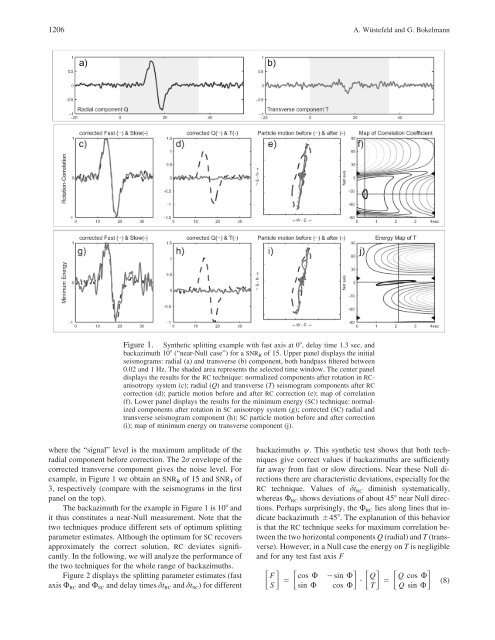
1206 A. Wüstefeld and G. BokelmannFigure 1. Synthetic splitting example with fast axis at 0, delay time 1.3 sec, andbackazimuth 10 (“near-Null case”) for a SNR R of 15. Upper panel displays the initialseismograms: radial (a) and transverse (b) component, both bandpass filtered between0.02 and 1 Hz. The shaded area represents the selected time window. The center paneldisplays the results for the RC technique: normalized components after rotation in RCanisotropysystem (c); radial (Q) and transverse (T) seismogram components after RCcorrection (d); particle motion before and after RC correction (e); map of correlation(f). Lower panel displays the results for the minimum energy (SC) technique: normalizedcomponents after rotation in SC anisotropy system (g); corrected (SC) radial andtransverse seismogram component (h); SC particle motion before and after correction(i); map of minimum energy on transverse component (j).where the “signal” level is the maximum amplitude of theradial component before correction. The 2r envelope of thecorrected transverse component gives the noise level. Forexample, in Figure 1 we obtain an SNR R of 15 and SNR T of3, respectively (compare with the seismograms in the firstpanel on the top).The backazimuth for the example in Figure 1 is 10 andit thus constitutes a near-Null measurement. Note that thetwo techniques produce different sets of optimum splittingparameter estimates. Although the optimum for SC recoversapproximately the correct solution, RC deviates significantly.In the following, we will analyze the performance ofthe two techniques for the whole range of backazimuths.Figure 2 displays the splitting parameter estimates (fastaxis U RC and U SC and delay times dt RC and dt SC ) for differentbackazimuths w. This synthetic test shows that both techniquesgive correct values if backazimuths are sufficientlyfar away from fast or slow directions. Near these Null directionsthere are characteristic deviations, especially for theRC technique. Values of dt RC diminish systematically,whereas U RC shows deviations of about 45 near Null directions.Perhaps surprisingly, the U RC lies along lines that indicatebackazimuth 45. The explanation of this behavioris that the RC technique seeks for maximum correlation betweenthe two horizontal components Q (radial) and T (transverse).However, in a Null case the energy on T is negligibleand for any test fast axis F F cos U sin U Q Q cos U • (8)S sin U cos U T Q sin U