Null Detection in Shear-Wave Splitting Measurements

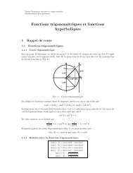
1206 A. Wüstefeld and G. BokelmannFigure 1. Synthetic splitting example with fast axis at 0, delay time 1.3 sec, andbackazimuth 10 (“near-Null case”) for a SNR R of 15. Upper panel displays the initialseismograms: radial (a) and transverse (b) component, both bandpass filtered between0.02 and 1 Hz. The shaded area represents the selected time window. The center paneldisplays the results for the RC technique: normalized components after rotation in RCanisotropysystem (c); radial (Q) and transverse (T) seismogram components after RCcorrection (d); particle motion before and after RC correction (e); map of correlation(f). Lower panel displays the results for the minimum energy (SC) technique: normalizedcomponents after rotation in SC anisotropy system (g); corrected (SC) radial andtransverse seismogram component (h); SC particle motion before and after correction(i); map of minimum energy on transverse component (j).where the “signal” level is the maximum amplitude of theradial component before correction. The 2r envelope of thecorrected transverse component gives the noise level. Forexample, in Figure 1 we obtain an SNR R of 15 and SNR T of3, respectively (compare with the seismograms in the firstpanel on the top).The backazimuth for the example in Figure 1 is 10 andit thus constitutes a near-Null measurement. Note that thetwo techniques produce different sets of optimum splittingparameter estimates. Although the optimum for SC recoversapproximately the correct solution, RC deviates significantly.In the following, we will analyze the performance ofthe two techniques for the whole range of backazimuths.Figure 2 displays the splitting parameter estimates (fastaxis U RC and U SC and delay times dt RC and dt SC ) for differentbackazimuths w. This synthetic test shows that both techniquesgive correct values if backazimuths are sufficientlyfar away from fast or slow directions. Near these Null directionsthere are characteristic deviations, especially for theRC technique. Values of dt RC diminish systematically,whereas U RC shows deviations of about 45 near Null directions.Perhaps surprisingly, the U RC lies along lines that indicatebackazimuth 45. The explanation of this behavioris that the RC technique seeks for maximum correlation betweenthe two horizontal components Q (radial) and T (transverse).However, in a Null case the energy on T is negligibleand for any test fast axis F F cos U sin U Q Q cos U • (8)S sin U cos U T Q sin U

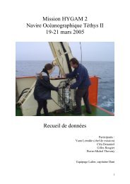
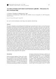
1208 A. Wüstefeld and G. Bokelmann|DU| 45/2. Near Null directions the RC delay times arebiased toward zero. The backazimuth with minimum dt RC isthus a further indicator of a Null direction (Fig. 2). Teleseismicnon-Null measurements thus require the followingcriteria: (1) the ratio of delay-time estimates from the twotechniques (q dt RC /dt SC ) is larger than 0.7 and (2) thedifference between the fast-axis estimates of both techniques,|DU|, is smaller than 22.5. Events with SNR T 3are classified as Nulls.Wolfe and Silver (1998) remark that waveforms containingenergy at periods (T) less than ten times the splittingdelays are required to obtain a good measurement. However,the arc-shaped pattern of dt RC persists for smaller delaytimes. Thus, the characteristics of the backazimuthal plots(as discussed previously) can provide valuable additional informationon the anisotropic parameters.Detecting Nulls using a data-based criterion providesthree advantages. First, it eliminates subjective measuressuch as evaluating initial particle motion and resulting energymap. Second, by varying the threshold values of DUand q, the user can change the sensitivity of Null detection.And third, the separation of Nulls is necessary for futureautomated splitting approaches. Because available data increaserapidly, the automation of the splitting process is adesirable goal in future applications and procedures.Quality DeterminationWe furthermore use the difference between results fromthe two techniques as a quality measure of the estimation.Again, such a data-based measure is more objective thanvisual quality measures based on seismogram shape and linearization(Barruol et al., 1997). In Figure 3 we compare,similar to Levin et al. (2004), both techniques by plottingthe difference of fast-axis estimates (|DU|) versus ratio ofdelay times (q dt RC /dt RC ) of synthetic seismograms.Based on the synthetic measurements (Fig. 2), we defineas good splitting measurements if 0.8 q 1.1 and DU 8 and fair splitting if 0.7 q 1.2 and DU 15. Nullmeasurements are identified as differences in fast-axis estimatesof about 45 and a small delay-time ratio q. Near thetrue Null directions the SC fast axis estimates are more robustthan the RC technique (Fig. 2). A differentiation betweenNulls and near-Nulls is useful in the interpretation ofbackazimuthal plots (Fig. 2). Good Nulls are characterizedby a small time ratio (0 q 0.2) and, following equationFigure 3. Misfit of delay-time and fast-axis estimates between RC and the SC techniquescalculated for 3185 synthetic seismograms at five different SNR R values between3 and 30 and seven input delay times between 0 and 2 sec from all backazimuths. TheNull criterion helps to identify Null measurements and at the same time gives a qualityattribute. Fair Null measurements are equivalent to near, Nulls.

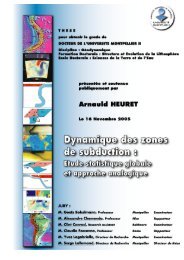
Null Detection in Shear-Wave Splitting Measurements 1209(9), a difference in fast axis estimate close to 45, that is 37 DU 53. Near-Null measurements can be classified by0 q 0.3 and 32DU 58. Remaining measurementsare to be considered as poor quality (see Fig. 3 for furtherillustration).Real DataWe apply our Null criterion to the shear-wave splittingmeasurements of station LVZ in northern Scandinavia. Theanalyzed earthquakes (M w 6) occurred between December1992 and December 2005. The data were processed by usingthe SplitLab environment (A. Wüstefeld et al., unpublishedmanuscript, 2006). This allows us to analyze eventsefficiently and to calculate simultaneously both the RC andSC technique. We mostly used raw data or, where necessary,applied third-order Butterworth bandpass filters with uppercornerfrequencies down to 0.2 Hz. Most usable events havebackazimuths between 45 and 100. Such sparse backazimuthalcoverage is unfortunately the case for many splittinganalyses, and we aim to extract the maximum informationabout the splitting parameters from these sparse distributions.In total we analyzed 37 SKS phases from a wide rangeof backazimuths (Fig. 4). Many results resemble Null characteristicsby showing low energy on the initial transversecomponent, elongated to linear initial particle motion and atypical energy plot. Such characteristics can be replicated insynthetic seismograms with near-Null parameters, that is,when the fast axis deviates less then 20 from backazimuth(Fig. 1). The average fast axis of the good events, as detectedautomatically and manually, is 14.3 and 14.7 for the SCand RC technique, respectively. Such orientation impliesNulls at backazimuths of approximately 15, 105, 195, and285 and favorable backazimuths for splitting measurementsin between. Indeed, good and fair splitting measurementsare found in backazimuthal ranges between 50 and 70 (Table1 and Fig. 4), where the energy on the transverse componentis expected to reach maximum possible values (seeequation 3) and the splitting can be inverted most reliably.Figure 4. Shear-wave splitting estimates from 33 good and fair measurements fromstation LVZ. The upper panels display fast-axis estimates for RC and SC methods. Notethat many RC estimates are situated near the dotted lines that indicate 45. The lowerpanels display the delay-time estimates. The solid horizontal lines indicate our interpretationof the LVZ with fast axis at 15 and 1.1-sec delay time, based on the meanof the good splitting measurements.

1210 A. Wüstefeld and G. BokelmannTable 1Good Events of Station LVZ as Detected AutomaticallyDate Lat Long Bazi* U SC U RC dt SC dt RC SNR SC†corr RC‡01-Oct-1994 17.75 167.63 55.1 19.1 13.1 0.8 0.8 5.85 0.8917-Mar-1996 14.7 167.3 54.3 14.3 12.3 1.0 1.0 9.55 0.9305-Apr-1997 6.49 147.41 71.1 17.1 24.1 1.4 1.3 6.16 0.8806-Feb-1999 12.85 166.7 54.2 6.2 11.2 1.2 1.2 10.43 0.9710-May-1999 5.16 150.88 67.3 11.3 10.3 1.3 1.3 5.70 0.8706-Feb-2000 5.84 150.88 67.5 13.5 13.5 1.4 1.4 9.33 0.9118-Nov-2000 5.23 151.77 66.5 18.5 18.5 1.0 1.0 5.74 0.90*Bazi, backazimuth† SNR SC , signal-to-noise ratio of the SC technique.‡ corr RC , correlation coefficient of the RC technique.Also in good agreement are the detected Nulls at backazimuthsbetween 80 and 110 and at about 270.Simultaneously, RC delay times systematically tend tosmaller values between backazimuths of 80 and 110, mimickingthe trapezoidal shape in the synthetic RC delay times(Fig. 2). Mean delay time estimates of good SC and RC are1.2 and 1.1 sec. respectively.Discussion and ConclusionsWe have presented a novel criterion for identifying Nullmeasurements in shear-wave splitting data based on two independentand commonly used splitting techniques. The twotechniques behave very differently near Null directions,where the RC technique systematically fails to extract thecorrect values both for the fast-axis azimuth U RC and delaytime dt RC . That technique should therefore not be used as a“stand-alone” technique. On the other hand, the comparisonof the two techniques is valuable for finding Null events.The backazimuths of Nulls ambiguously indicates either fastor slow direction. Thus, a Null measurement yields limited,yet important, constraints on anisotropy orientation, especiallyif the backazimuthal coverage of the station is onlysparse. Furthermore, Nulls from a wide range of backazimuthsindicate either the lack of (azimuthal) anisotropy orweak anisotropy, at the limit of detection. Restivo and Helffrich(1998) analyzed the splitting procedure for effects ofnoise. They conclude that for small splitting filtering doesnot necessarily result in more confident estimates of splittingparameters, since narrow bandpass filters lead to apparentNull measurements. For SNR above 5 our criterion detectsNull measurements and classifies near-Nulls. Good eventscan still be obtained but only for exceptionally good SNR orwith backazimuths far away oriented with respect to theanisotropy axes (where the transverse amplitude is larger;see equation 3).The comparison of the two shear-wave splitting techniquesallows assigning a quality to single measurements(Fig. 1). Furthermore, the joint two-technique analysis of allmeasurements (Fig. 2) yields characteristic variations ofsplitting parameter estimates with backazimuth. This variationcan be used to extract the maximum information fromthe data, and to decide whether a more complex anisotropythan a single layer needs to be invoked to explain the observations.The practical steps for this should be: first, assumea single-layer case with the most probable fast directionbased on the good measurements. Second, verify thatNulls measurements occur near the corresponding Null directionsin the backazimuth plot (Fig. 4). In the vicinity ofthese Null directions, the splitting parameter estimates U SCand dt SC should show a larger scatter with a tendency towardlarge delays. For dt RC we expect to find an arc-shaped variationwith backazimuth that should have its minimums nearthe assumed Null directions. If these conditions are met, aone-layer case can reasonably explain the observations. Onthe other hand, good events that deviate from these predictionsmay require more complex anisotropy (multilayer caseor dipping layer). Applied to station LVZ in northern Scandinavia,we were thus able to comfortably characterize theanisotropy by a single anisotropic layer with a fast axis orientedat 15 and a delay time of 1.1 sec.ReferencesBarruol, G., P. G. Silver, and A. Vauchez (1997). Seismic anisotropy in theeastern US: Deep structure of a complex continental plate, J. Geophys.Res. 102, no. B4, 8329–8348.Bowman, J. R., and M. Ando (1987). Shear-wave splitting in the uppermantlewedge above the Tonga subduction zone, Geophys. J. R. Astr.Soc. 88, 25–41.Brechner, S., K. Klinge, F. Krüger, and T. Plenefisch (1998). Backazimuthalvariations of splitting parameters of teleseismic SKS phases observedat the broadband stations in Germany, Pure Appl. Geophys.151, 305–331.Chevrot, S. (2000). Multichannel analysis of shear wave splitting, J. Geophys.Res. 105, no. B9, 21,579–21,590.Currie, C. A., J. F. Cassidy, R. D. Hyndman, and M. G. Bostock (2004).Shear wave anisotropy beneath th Cascadia subduction zone and westernNorth American Craton, Geophys. J. Int. 157, 341–353.Fouch, M. J., K. M. Fischer, E. M. Parmentier, M. E. Wysession, and T. J.Clarke (2000). Shear wave splitting, continental keels, and patternsof mantle flow, J. Geophys. Res. 105, no. B3, 6255–6275.Fukao, Y. (1984). Evidence from core-reflected shear waves for anisotropyin the earth’s mantle, Nature 309, 5970, 695.Levin, V., D. Droznin, J. Park, and E. Gordeev (2004). Detailed mapping

Null Detection in Shear-Wave Splitting Measurements 1211of seismic anisotropy with local shear waves in southeastern Kamchatka,Geophys. J. Int. 158, no. 3, 1009–1023.Menke, W., and V. Levin (2003). The cross-convolution method for interpretingSKS splitting observations, with application to one and twolayeranisotropic earth models, Geophys. J. Int. 154, no. 2, 379–392.Nicolas, A., and N. I. Christensen (1987). Formation of anisotrophy inupper mantle peridotites: a review, in Composition Structure and Dynamicsof the Lithosphere Asthenosphere System, K. Fuchs and C.Froideveaux (Editors), American Geophysical Union, Washington,D.C., 111–123.Ozalaybey, S., and M. K. Savage (1994). Double-layer anisotropy resolvedfrom S phases, Geophys. J. Int. 117, 653–664.Restivo, A., and G. Helffrich (1999). Teleseismic shear wave splitting measurementsin noisy environments, Geophys. J. Int. 137, no. 3, 821–830.Saltzer, R. L., J. B. Gaherty, and T. H. Jordan (2000). How are verticalshear wave splitting measurements affected by variations in the orientationof azimuthal anisotropy with depth? Geophys. J. Int. 141,374–390.Savage, M. K. (1999). Seismic anisotropy and mantle deformation: whathave we learned from shear wave splitting, Rev. Geophys. 37, 69–106.Silver, P. G., and W. W. Chan (1991). Shear wave splitting and subcontinentalmantle deformation, J. Geophys. Res. 96, no. B10, 16,429–16,454.Teanby, N., J. M. Kendall, and M. van der Baan (2003). Automation ofshear-wave splitting measurements using cluster analysis, Bull. Seism.Soc. Am. 94, 453–463.Vinnik, L. P., V. Farra, and B. Romanniwicz (1989). Azimuthal anisotropyin the earth from observations of SKS at GEOSCOPE and NARSbroadband stations, Bull. Seism. Soc. Am. 79, no. 5, 1542–1558.Wolfe, C. J., and P. G. Silver (1998). Seismic anisotropy of oceanicupper mantle: Shear wave splitting methodologies and observations,J. Geophys. Res. 103, no. B1, 749–771.Geosciences MontpellierUniversité de Montpellier II34095 Montpellier, Francewueste@gm.univ-montp2.frbokelmann@gm.univ-montp2.frManuscript received 19 September 2006.