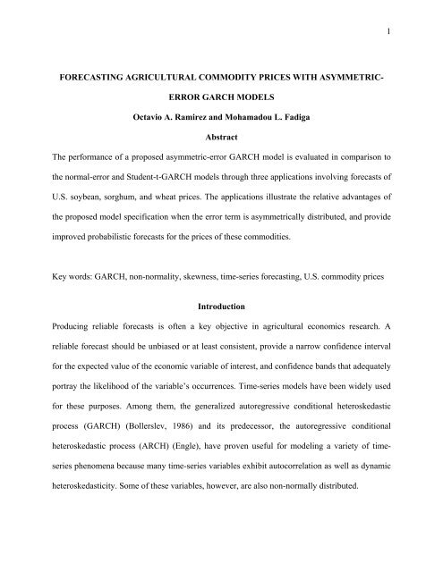
forecasting agricultural commodity prices with asymmetric-error ...

1FORECASTING AGRICULTURAL COMMODITY PRICES WITH ASYMMETRIC-ERROR GARCH MODELSOctavio A. Ramirez and Mohamadou L. FadigaAbstractThe performance of a proposed asymmetric-error GARCH model is evaluated in comparison tothe normal-error and Student-t-GARCH models through three applications involving forecasts ofU.S. soybean, sorghum, and wheat prices. The applications illustrate the relative advantages ofthe proposed model specification when the error term is asymmetrically distributed, and provideimproved probabilistic forecasts for the prices of these commodities.Key words: GARCH, non-normality, skewness, time-series forecasting, U.S. commodity pricesIntroductionProducing reliable forecasts is often a key objective in agricultural economics research. Areliable forecast should be unbiased or at least consistent, provide a narrow confidence intervalfor the expected value of the economic variable of interest, and confidence bands that adequatelyportray the likelihood of the variable’s occurrences. Time-series models have been widely usedfor these purposes. Among them, the generalized autoregressive conditional heteroskedasticprocess (GARCH) (Bollerslev, 1986) and its predecessor, the autoregressive conditionalheteroskedastic process (ARCH) (Engle), have proven useful for modeling a variety of timeseriesphenomena because many time-series variables exhibit autocorrelation as well as dynamicheteroskedasticity. Some of these variables, however, are also non-normally distributed.

2Agricultural economics applications of standard GARCH models include Moss, andMoss, Shonkwiler, and Ford. Bollerslev (1987) proposed a non-normal-error GARCH model ofspeculative prices and rates of return based on the Student-t distribution (t-GARCH), which isleptokurtic but symmetric. Yang and Brorsen, concerned with the non-normality of daily cashprices, explored the use of a mixed diffusion-jump process, a deterministic chaos model, and thet-GARCH model to explain the stochastic behavior of these prices. Yang and Brorsen (p. 714)concluded that, while the t-GARCH model best explains daily cash price behavior, “it is not wellcalibrated” because it cannot explain all of the observed non-normality, referring to the t-GARCH model’s inability to account for the skewness in the distribution of cash prices.Pagan and Sabau, Lee and Hansen, and Deb have shown that, in finite sample sizes,misspecification of the error-term distribution results in poor statistical properties, and anunreliable quasi-maximum likelihood estimator. Ramirez and Shonkwiler report that symmetricerrorGARCH models tend to underestimate the true standard errors of the intercept and slopeparameter estimators when the true underlying error-term distribution is asymmetric. Becausemost GARCH applications occur with small- or moderate-sized samples, a flexible specificationthat can accommodate both error-term skewness and kurtosis is important to improve thereliability of quasi-maximum likelihood estimation of GARCH models.To address the problem of unreliable quasi-maximum likelihood estimation of GARCHmodels, Wang et al. recently proposed an asymmetric-error GARCH model based on theExponential Generalized Beta 2 (EGB2) family of distributions and used it for the modeling ofexchange rates. According to McDonald and White, however, the EGB2 can only accommodatepositive standardized (normal kurtosis = 0) kurtosis coefficients from 0 to 6, and skewness

4Where -∞

5but symmetric error GARCH versus the alternative of a full (leptokurtic and skewed error) A-GARCH is given by H 0 : Θ>0, µ=0 vs. H A : Θ>0, µ≠0. The null of an N-GARCH versus thealternative of a full A-GARCH can be directly tested as well.Another advantage of the A-GARCH is that the degree of skewness and kurtosis of theerror-term distribution can be assumed variable across observations without interfering with theestimation of the linear regression and GARCH-process parameters. This is achieved by makingeither Θ, µ, or both, a function of time or any other potentially relevant factor. Given equations(1) and (2), the concentrated log-likelihood function for estimating the A-GARCH model isobtained using the transformation technique (Mood, Graybill, and Boes):TT(6) LL = Σ ln(G t ) −0.5×Σ H 2 t ;t=1 t=1where: G t ={h t /G(Θ,µ)(1+R t 2 )} -1/2 , H t ={sinh –1 (R t )/Θ}−µ, R t =[Θ(y t -x’ t b)/{h t /G(Θ,µ)} -1/2 ]+F(Θ,µ),t=1,…,T refers to the observations, sinh –1 (R t )=ln{R t +(1+ R t 2 ) 1/2 } is the inverse hyperbolic sinefunction, and h t , F(Θ,µ), and G(Θ,µ) are as given in equations (1) and (2).Maximization of (6) with respect to the model’s parameters is achieved throughnumerical optimization algorithms, which are available in most econometric software packages,including the Gauss-386i program used in this study. These pre-programmed procedures onlyrequire a few standard command lines and the log-likelihood function. These procedures achieveconvergence when the gradients of all parameter estimates are less than some arbitrarily smallamount. In addition to parameter estimates, they provide standard errors based on a numericalestimate of the Hessian matrix of this function. In most applications, the optimization algorithmconverges quickly and properly, as long as the starting values are reasonable. The intercept,

6slope, and GARCH process parameter estimates from an N-GARCH model are excellent startingvalues, while it is best to start with 0.1

7skewness, the A-GARCH allows for any possible mean-variance-leptokurtosis combination: itcan precisely fit the first four central moments of any symmetric “thick”-tailed distribution.Normal-Error versus t- and A-GARCH Models of U.S. Commodity PricesThe modeling strategy of Engle and Kraft, also used by Bollerslev (1986) to illustrate hisGARCH expansion of Engle’s ARCH process, is adopted here. In particular, it is assumed thatreal U.S. commodity prices may be forecasted on the basis of their past behavior:(7) P t = b 0 + b 1 P t-1 + b 2 P t-2 + b 3 P t-3 + b 4 P t-4 + ε t , ε t ∼ NN(0,h t ), h t = α 0 + α 1 ε 2 t-1 + β 1 h t-1.All models are estimated using the Newton-Raphson algorithm (cubic step-lengthcalculation method) preprogrammed in Gauss 386i constrained maximum likelihood (CML)module. The model in equation (7) is first estimated for real, quarterly U.S. soybean (1924-2000), sorghum (1933-2000), and wheat (1913-2000) prices received by farmers, under theassumption of error-term normality. These nominal price data were compiled from the USDANational Agricultural Statistics Service (NASS) database (http://www.usda.gov/nass/pubs/histdata.htm). They were adjusted for inflation, with year 2000 as a base, using the producerprice index for non-processed agricultural products from the U.S. Department of Labor, Bureauof Labor Statistics (http://www.bls.gov/).All price series are found to be stationary according to augmented Dickey-Fuller tests.Also following Bollerslev (1986), the standardized GARCH residuals (ε t /h ½ t ) are tested forindependence. In the case of soybeans and wheat, several autocorrelations and partialautocorrelations are statistically significant at the 5% level, and the Box-Pierce Q statistic rejectsthe null hypotheses that the first twelve autocorrelation coefficients are all zero, also at the 5%level. In the case of sorghum, only the seventh partial autocorrelation is significant at the 5%level, but the Q statistic does not reject the joint null hypothesis of error-term independence at

8the 10% level. Closer examination of the correlograms suggests that the autocorrelation patternsin the residuals or the soybean and wheat models are likely due to seasonality.Therefore, the data are seasonally adjusted following a standard centered multiplicativemoving-average procedure. The deseasonalized data are also stationary, according to augmentedDickey-Fuller tests. N-, t- and A-GARCH models are then estimated with the deseasonalizedprice data. In the case of soybean and wheat prices, the standardized residuals do not show anystatistically significant autocorrelations, partial autocorrelations, or Q statistics, at the 10% level.Deseasonalizing real prices solves the autocorrelation problem. Because deseasonalizing actuallycreates a residual autocorrelation problem in the case of sorghum, the models are estimated withseasonally adjusted soybean and wheat data, and with the unadjusted sorghum data (Table 1).All GARCH parameters (α 0 α 1 and β 1 ) are statistically different from zero at the 5% leveland all models satisfy the variance stationarity condition (0

9transformation of a normal, the residuals from the t-GARCH models can be standardized but notnormalized, which makes it difficult to ascertain how well the t distribution is able to modelerror-term non-normality in a particular application.Under the null hypothesis of normality, S and K are distributed approximately normal,and K 2 follows a χ 2 (2) distribution. Note that, in the N-GARCH models, the null hypotheses ofresidual normality are rejected at the 1% level of statistical significance in all three cases. The Sand K statistics indicate statistically significant error-term skewness and kurtosis in the case ofsoybean and sorghum prices, but only kurtosis in the case of wheat prices (Table 1).Fully parameterized A-GARCH models (available from the authors) were initiallyestimated specifying the kurtosis and the skewness parameters (θ and µ) as linear functions oftime (θ t = θ 0 + θ 1 t and µ t = µ 0 + µ 1 t). Single-parameter likelihood ratio (LR) (χ 2 (1)) tests and theusual t-tests are conducted separately to ascertain the statistical significance of θ 0 , θ 1 , µ 0 and µ 1 .As expected, the LR and the t tests yield similar results. The final A-GARCH models presentedin Table 1 were obtained by setting any of these four parameters (θ 0 , θ 1 , µ 0 , or µ 1 ) that did notresult statistically significant at the 10% level equal to zero. As a result, the final models forsoybean, sorghum, and wheat prices only include θ 1 , µ 0 , and µ 1 , θ 0 and µ 0 , and θ 0 , respectively.In the case of soybean prices, θ 0 =0 implies that the error-term distribution was nearlynormal during the 1920s. The positive estimate for θ 1 combined with a negative estimate for µ 1in this case results in the kurtosis coefficient increasing through time at a faster rate than theskewness coefficient. Specifically, the skewness and kurtosis coefficients, calculated using theformulas in equations (4) and (5), are both below 0.5 until 1943. By 1960, skewness reaches 1.2and kurtosis 6.26. The estimated year 2000 error-term distribution is considerably skewed (3.34)and highly kurtotic (53.27).

10In the final A-GARCH sorghum price model, θ 1 =0 and µ 1 =0, but θ 0 and µ 0 arestatistically different from zero. The positive estimate for µ 0 , implies a right-skewed andleptokurtic error distribution with constant skewness and kurtosis coefficients of 1.46 and 9.84,respectively. Note that some of these skewness-kurtosis combinations are not allowed by theEGB2 family. The EGB2-GARCH would not be as theoretically suitable to model soybean andsorghum prices. In the final A-GARCH wheat model, only θ 0 is statistically different from zero,implying an error-term distribution with a constant kurtosis coefficient of 3.78.In short, two of the three estimated A-GARCH models exhibit error-term distributionsthat are substantially right-skewed, implying that relatively high positive forecasting errors aremore likely than negative errors of the same high magnitude. Right skewed forecasting errors areexpected because agricultural price series, even when expressed in real terms, usually exhibitmore pronounced peaks on the up side than on the down side. In all three cases, likelihood ratiotests (χ 2 (3) = 113.06−65.67 = 47.39; χ 2 (2) = 69.40−1.97 = 67.43; χ 2 (1) = 472.59−449.86 = 22.73)rejected H 0 : θ 1 =µ 0 =µ 1 =0, H 0 : θ 0 =µ 0 =0, and H 0 : θ 0 =0 at the 1% level (Table 1), implying that thefinal A-GARCH models are significantly more likely to have generated the observed soybean,sorghum, and wheat price data than final N-GARCH models.Also note that the values taken by the S, K and K 2 statistics for the standardized andnormalized residuals from the final A-GARCH models are all less than one. This indicates the“normalizing” transformation implied by the expanded S U family was successful in removing thenon-normality from the GARCH residuals in all cases. In other words, the expanded S U familyprovides a good approximation to the non-normal distribution of those residuals.Initial t-GARCH models were also estimated assuming that the degrees of freedomparameter (θ), which determines the degree of leptokurtosis of the error-term distribution, was a

11function of time (θ t = θ 0 + θ 1 t). As before, the final t-GARCH models were obtained by setting tozero any of the two parameters (θ 0 or θ 1 ) not statistically significant at the 10% level (Table 1).θ 1 is only significant in the case of the soybeans model, resulting in the degrees-of-freedomparameter declining from 7.8 in 1924 to 2.1 in the 2000. As in the A-GARCH model of soybeanprices, the kurtosis coefficient is markedly increasing through time. Also as in the A-GARCHmodels, the error-term kurtosis in the t-GARCH models of sorghum and wheat prices hasremained constant though time.The t-GARCH approaches an N-GARCH as the degrees-of-freedom parameter (θ)approaches infinity, that is, at the boundary of the admissible parameter space. This relationshipimplies the distribution of a likelihood ratio test statistic in which the N-GARCH is viewed as arestricted t-GARCH would be more concentrated towards zero than the probability distributionof a χ 2 (1) variable (Bollerslev, 1987). It follows that rejection of H 0 : N-GARCH in favor of H A : t-GARCH by comparing the likelihood ratio test statistic with a χ 2 (1) (or a χ 2 (2), when θ = θ t = θ 0 +θ 1 t) would be safe conclusion. Such likelihood ratio tests allow for rejection of H 0 : N-GARCH infavor of H A : t-GARCH in all three commodity price models (χ 2 (2) = 93.62−65.67 = 27.95; χ 2 (1) =56.65−1.97 = 54.68; and χ 2 (1) = 471.33−449.86 = 21.47).In regards to forecasting performance, because of the partially adaptive nature of the A-GARCH models (Mc Donald and White), the standard error estimates for the intercept and“slope” parameters (b 1 , b 2 , b 3 , b 4 , b 5 , and b 6 ) in these models are always and sometimessubstantially lower than in the N-GARCH models. Also note that the standard error estimateshave to be evaluated in light of the previously discussed evidence about the unreliability ofquasi-maximum likelihood estimation results when working with finite samples and amisspecified error-term distribution. In particular, symmetric-error GARCH models tend to

12underestimate the true standard errors of the intercept and slope parameter estimators when thetrue underlying error-term distribution is asymmetric. Given the A-GARCH is based on the mostflexible error-term distribution, and that statistically significant skewness is detected in the caseof soybean and sorghum prices, the A-GARCH standard error estimates should be consideredmore reliable than those of the N- and t-GARCH models. The latter models likely underestimatethe true standard errors. In the absence of significant skewness, as in the case of wheat price, thet- and A-GARCH models yield nearly identical results.Because of the differences in the intercept and slope parameter estimates, the pointforecasts from the N- t- and A-GARCH models differ noticeably from each other. Specifically,the averages of the absolute differences between the within-sample forecasts from the N- versusthe A-GARCHs are 5.4, 6.8, and 1.8 cents/bushel in the case of the soybean, sorghum, and wheatmodels, respectively, while the maximum differences are 35, 46, and 10 cents/bushel,respectively. Interestingly, larger average absolute differences are found between the N- and A-GARCH models in which the error-terms exhibit more pronounced non-normality. In spite of thelarge average absolute differences, the within-sample root mean square prediction errors (RMSE)and the squares of the correlation coefficients between the observed and the predicted dependentvariable values (R 2 s) are almost identical under these three types of models (Table 2). Nearlyequal RMSEs, however, do not imply that the N-, t-, and A-GARCH model predictions and theirassociated confidence intervals are equally reliable.A reliable prediction is characterized by narrow and accurate confidence intervals for thedependent variable occurrences. In non-linear models, confidence intervals are usually obtainedby applying the numerical technique of Krinsky and Robb. Specifically, let Ê i (i=N, t, or A) bethe kx1 vector of maximum likelihood estimators for E i , the vector of true population parameters

13underlying the N-, t-, or A-GARCH models, and ECM[Ê i ] be the (kxk) estimated covariancematrix for Ê i . Then, a draw from the joint probability distribution of Ê i is simulated by:(8) Z x Chol(ECM[Ê i ]) + Ě i , (i=N, t, or A)where Z is a 1xk vector of independent standard normal draws, Chol(.) denotes the Choleskydecomposition, and Ě i the 1xk vector of ML parameter estimates obtained from Ê i . Repeatedapplication of equation (8) yields an mxk matrix (S i ) of random variables with mean Ě i andcovariance matrix ECM[Ê i ]. Under the correct model specification, Ê i is a consistent estimatorfor E i and ECM[Ê i ] is a consistent estimate for the covariance matrix (CM[Ê i ]), implying S i is atheoretically correct probabilistic statement about E i . Thus, the boundaries of a (1-α)%confidence interval for the expected soybean, sorghum, corn and wheat prices under the N-, t- orA-GARCH models at time period t can be obtained by extracting the m sets of simulatedintercept and slope parameter values from S N , S t , or S A to obtain m “predicted” price values fortime t, and finding the (α/2) x m th and the [(1-α)+α/2] x m th largest of these m price values.The next step in computing the confidence intervals for the actual price occurrencesrequires simulation of m draws of the error-term as well. In the case of the N-GARCH, these areobtained by extracting the m simulated values for the GARCH process parameters (α 0 , α 1 , andβ 1 ) from S N and using them to obtain m simulated values of h t according to the GARCH(1,1)variance function [equation (7)], and multiplying their square roots by m independent draws froma standard normal random variable. In the case of the A and t-GARCH models, the process ofsimulating the h t values is similar, except that the m sets of simulated GARCH processparameters are extracted from S A and S t .For the A-GARCH, these m simulated h t values are coupled with the m simulated Θ 0 , µ 0 ,Θ 1 , and µ 1 values, also obtained from S A , and with m independent standard normal draws. Then,

14m non-normal error-term values are simulated by applying equation (2). For the t-GARCH, thesquare roots of the m simulated h t values are coupled with the m simulated Θ 0 and Θ 1 valuesobtained from S t , and multiplied by m independent draws from a Student t distribution with Θ 0 +Θ 1 t degrees of freedom. The final step in constructing the boundaries of a (1-α)% confidenceinterval for the actual price observations is to add the m simulated error-term values to thecorresponding m simulated price “predictions” and find the (α/2) x m th and the [(1-α)+α/2] x m thlargest of the resulting m simulated price realization values.The process described above is programmed in Gauss 386i with m=10,000, starting at t=1assuming ε 0 =0 and h 0 = α 0 /(1-α 1 -β 1 ) (the unconditional GARCH process variance), andrecursively repeated up to t=T, under the N-, t-, and A-GARCH soybean, sorghum, and wheatprice models. The resulting boundaries are joined to obtain (1-α)% confidence bands for the Twithin-sample price predictions from each of the estimated models. The process is repeated fromα=0.20 to α=0.01 at 0.01 decrements to obtain 80% to 99% confidence bands.Figure 1 shows the 80% confidence bands for the soybean price occurrences versus thesample data under the N- and A-GARCH models. The difference between these two confidencebands starts to become visually obvious at about 1950, when the estimated error-term becomessubstantially non-normal. Under the N-GARCH, the observed prices tend to be closer to themiddle of the interval. Only 19 observations trespass the lower bound, while 30 observationsexceed the upper bound of the 80% confidence band, versus the theoretically required T*0.20/2 =304*0.20/2 = 30.4. Given the pattern of the soybean price observations, the symmetry of theassumed error-term distribution results in a lower bound that is unnecessarily low in order toensure that more of the observed price spikes do not surpass the upper bound.

15Under the A-GARCH, the right-skewness in the estimated error-term distribution allowsfor a substantially higher lower bound, which is closer to the mass of the observations, coupledwith an upper bound that is still high enough to avoid a theoretically excessive number ofobservations surpassing it. Specifically, 25 observations are found under the lower bound and 35exceed the upper bound of the 80% confidence band, respectively, versus the theoreticallyrequired 30.4. The t-GARCH bands are symmetric, like the N-GARCH bands, and follow asimilar visual pattern. The 80% band leaves 20 observations under its lower bound and 41observations above its upper bound. At the same time, the average width of the 80% A-GARCHband is $1.35/bushel, versus $1.51/bushel for the N-GARCH and $1.41/bushel in the t-GARCH.Figure 2 shows the number of observations left below the lower bounds of the 80 to 99%confidence bands from the N-, t-, and A-GARCH models of soybean prices, versus thetheoretically required numbers. Both the N- and the t-GARCH bands leave substantially fewerobservations under their lower bounds than required; while leaving an excessive number ofobservations over their upper bounds.When all 20 (80 to 99%) confidence bands are jointly considered, only 164 (51.4%) out20of the theoretically required total of (Tx∑ i /100 )/2 = (304x i /100 )/2 = 319 (100%)i=1observations are found below the lower bounds of the N-GARCH, while 414 observations(129.7%) appear above the upper bounds (Table 2). In the case of the t-GARCH, 169 (or 52.9%of the theoretically required) are found below the lower bounds, and 422 (132.2%) appear abovethe upper bounds. The assumption of error-term symmetry, which causes these confidence bandsto be symmetric about the predictions, is clearly incompatible with the observed soybean pricedata. The 80 to 99% A-GARCH bands, in contrast, leave a total of 286 (89.6%) observations20∑i=1

16below and 379 (118.7%) observations above their respective boundaries. Although not perfect,the A-GARCH bands adhere more closely to what is theoretically expected.The A-GARCH bands, being kurtotic and non-symmetric about the predictions becauseof the leptokurtosis and right-skewness of the estimated error-term distribution, better reflect thestatistical behavior of soybean prices. At the same time, the average width of the A-GARCHconfidence bands is $1.96/bushel, versus $2.03/bushel and $2.25/bushel in the case of the N- andt-GARCH bands. As illustrated in Figure 1, compatibility with the data is improved by lowerbounds that are higher than their N- and t-GARCH counterparts, and thus closer to the mass oflow price occurrences, combined with upper bounds that are similar to the N-GARCH’s at highαs but become relatively higher at reduced α levels.As illustrated in Figure 3, the A-GARCH confidence bands for the sorghum priceoccurrences are also more compatible with the observed data than the bands under the N- and t-GARCH models. The 80 to 99% N-GARCH bands leave a total of 100 (35.7%) and 273 (97.4%)out of the theoretically required (267x20∑i=1i /100 )/2 = 280 (100%) observations below and abovetheir lower and upper bounds, respectively, while the t-GARCH bands leave 189 (67.4%) and439 (156.6%) observations below and above their lower and upper bounds, respectively. Incontrast, in the case of the A-GARCH 253 (90.2%) and 284 (101.3%) observations are left belowand above the lower and upper bounds, respectively (Table 2).It could be argued that the N-GARCH bands in this case could be narrower, leaving moreobservations below and above their boundaries. However, although the 80% band is much widerthan theoretically desired, the 95% and 99% bands leave 3.4% and 2.2% of the observationsabove their upper bounds (Table 2), i.e. they are much too narrow on the up side. The problemthen is that the normal distribution cannot produce bands that are asymmetric and narrower at

17high α values and wider at the lower α levels. Interestingly, the average width of the 80 to 99%confidence bands is less under the t-GARCH than the A-GARCH (Table 2). This is of noadvantage because the band locations are incompatible with the data, but it illustrates the findingof Wang et al. that when the underlying error-term is asymmetric, the t-GRACH tends tooverestimate the degree of kurtosis, fitting an excessively peaked distribution.In the case of the wheat prices, where the error-term appears to be symmetricallydistributed, the t- and A-GARCH models provide fairly similar results, as expected, while the N-GARCH still produces a less than adequate statistical representation of the data and relativelywide inefficient confidence bands for the price occurrences (Table 2).The previously discussed inconsistencies between the confidence bands implied by thesymmetric-error N- and t-GARCH models and the data that they are supposed to represent areimportant because a reliable, accurate confidence interval is an essential element of a goodprediction. The demonstrated incompatibility of the N- and t-GARCH confidence bands with thedata is also important because it illustrates the inadequacy of these models when the underlyingerror is asymmetrically distributed. Although the inadequacy of symmetric-error GARCHmodels when the true error-term distribution is asymmetric has been established in theory, thegood R 2 s and RMSEs for the forecasts often associated with these misspecified models mightdeceive applied researchers into thinking that they provide reliable predictions of the data.Concluding RemarksThe asymmetric-error GARCH model proposed and illustrated in this paper represents animproved alternative for the forecasting of time-series variables and for producing reliableconfidence intervals for these forecasts when the conditional probability distribution of thedependent variable is asymmetric. Researchers using GARCH models should test for error-term

18non-normality as illustrated in this paper. If the error-term appears leptokurtic but not skewed,either the t- or the A-GARCH model discussed in this paper should be utilized. If the testssuggest both positive kurtosis and right- or left-skewness, either the EGB2- or the A-GARCHcould be suitable, subject to the previously discussed limitations in the levels of skewness andkurtosis allowed by the EGB2 family of distributions. Unfortunately, no theoretically suitablealternative to model the less common negative (platy) kurtosis is available.Footnotes1 The A-GARCH is not directly compared to the EGB2-GARCH because the main means ofcomparison utilized in the paper, i.e. the computation of confidence bands for the dependentvariable occurrences, require simulation of random draws from the assumed error-termdistribution. To our knowledge, there are no procedures to simulate draws from an EGB2.

19ReferencesAptech Systems, Inc. Gauss-386i Mathematical and Statistical System. Maple Valley, WA, 1999.Bollerslev, T. “Generalized Autoregressive Conditional Heteroskedasticity.” Journal ofEconometrics 31(1986):307-27.Bollerslev, T. “A Conditionally Heteroskedastic Time-Series Model for Speculative Prices andRates of Return.” The Review of Economics and Statistics 69(August 1987):542-47.D’Agostino, R.B., A. Belanger, and R.B. D’Agostino Jr. “A Suggestion for Using Powerful andInformative Tests of Normality.” The American Statistician 44(4)(November 1990):316-21.Deb, P. 1996. Finite Sample Properties of Maximum Likelihood and Quasi-MaximumLikelihood Estimators of EGARCH Models.” Econometric Reviews 15:51-68.Engle, R.F. and D. Kraft. “Multiperiod Forecast Error Variances of Inflation Estimated fromARCH Models.” In Applied Time-series Analysis of Economic Data, ed., A. Zellner, pp. 93-302. Washington D.C.: Bureau of the Census, 1993.Engle, R.F. (1982). Autoregressive conditional heteroskedasticity with estimates of the variance ofU.K. inflation. Econometrica 50:987-1008.Johnson, N.L., S. Kotz, and N. Balakrishnan. Continuous Univariate Distributions. New York:Wiley & Sons, 1994.Krinsky, I., and A.L. Robb. “On Approximating the Statistical Properties of Elasticities.” Review ofEconomics and Statistics 68(1986):715-19.Lee, S., and B.E. Hansen. “Asymptotic Theory for the GARCH(1,1) Quasi-Maximum LikelihoodEstimator. Econometric Theory 10(1994):29-52.

20McDonald, J.B., and S.B. White. “A Comparison of Some Robust, Adaptive, and PartiallyAdaptive Estimators of Regression Models. Econometric Reviews 12(1)(1993):103-24.McDonald, J.B., and W.K. Newey. “Partially Adaptive Estimation of Regression Models Via theGeneralized t Distribution.” Econometric Theory 4(1988):428-57.Mood, A.M., F.A. Graybill, and D.C. Boes. Introduction to the Theory of Statistics. New York:McGraw-Hill, 1974.Moss, C.B. “The Cost Price Squeeze in Agriculture: An Application of Cointegration.” Review ofAgricultural Economics 14(1)(1992):209-217.Moss, C.B., J.S. Shonkwiler, and S.A. Ford. “A Risk Endogenous Model of AggregateAgricultural Debt.” Agricultural Finance Review 50(1990):73-79.Ramirez, O.A. and J.S. Shonkwiler. “Autoregressive Conditional Heteroskedasticity under Error-Term Non-Normality.” Texas Tech University, CASNR Manuscript No. 1-513, May2001.Pagan, A.R., and H. Sabau. “On the Inconsistency of the MLE in Certain HeteroskedasticRegression Models.” Mimeo, University of Rochester, 1987.U.S. Department of Agriculture (USDA), National Agricultural Statistics Service (NASS).NASS historical data. Online. Available at http://www.usda.gov/nass/pubs /histdata.htm.Retrieved January 2001.U.S. Department of Labor, Bureau of Labor Statistics. Online. Available at http://www.bls.gov/.Retrieved January 2001.Wang, K.L., C. Fawson, C.B, Barrett, and J.B. McDonald. “A Flexible Parametric GARCHModel with an Application to Exchange Rates.” Journal of Applied Econometrics 16(2002):521-36.

21Yang, S-R. and B.W. Brorsen. “Nonlinear Dynamics of Daily Cash Prices.” American Journal ofAgricultural Economics 74(3)(August 1992):706-15.