P Systems with Active Membranes Characterize PSPACE

P Systems with Active MembranesCharacterize PSPACEPetr Sosík a,b,∗ Alfonso Rodrígues-Patón Aradas aa Universidad Politécnica de Madrid – UPM, Faculdad de InformáticaCampus de Montegancedo s/n, Boadilla del Monte28660 Madrid, Spainb Institute of Computer Science, Silesian University74601 Opava, Czech RepublicAbstractP system is a natural computing model inspired by behavior of living cells andtheir membranes. We show that (semi-)uniform families of P systems with activemembranes can solve in polynomial time exactly the class of problems PSPACE.Consequently, these P systems are computationally equivalent (w.r.t. the polynomialtime reduction) to standard parallel machine models as PRAM and the alternatingTuring machine.Key words: Keywords: Natural computing, P system, PSPACE, alternatingTuring machine1 IntroductionThe computational power of P systems in active membranes was studied firstin [9], where their ability to solve NP-complete problems in polynomial timewas demonstrated. Later it was shown in [12,2] that (semi-)uniform familiesof deterministic P systems with active membranes can solve also the problemQBF (satisfiability of quantified propositional formulas) in a polynomial time.As QBF is a classical PSPACE-complete problem, any other problem inPSPACE can be also (after a reduction to QBF) solved in a polynomial timein the same way.∗ Corresponding author.Email addresses: petr.sosik@fpf.slu.cz (Petr Sosík), arpaton@fi.upm.es(Alfonso Rodrígues-Patón Aradas).Preprint submitted to Elsevier Science 18 December 2005

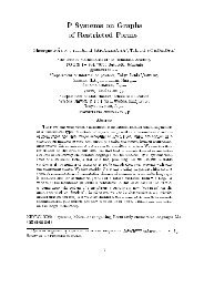
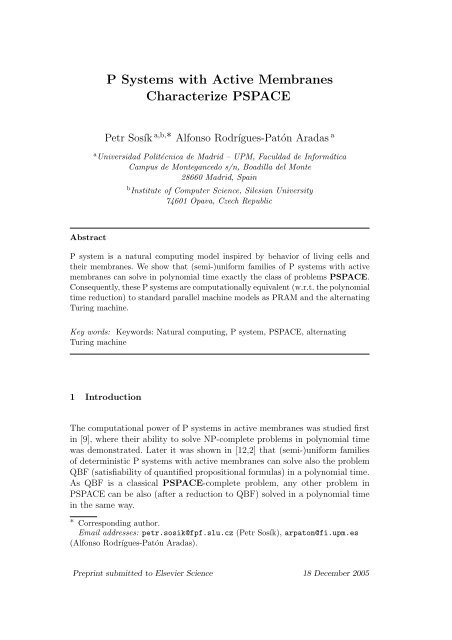
Here we complete the characterization of the computational power of P systemswith active membranes. We show that the class of problems solvable inpolynomial time by these P systems is exactly the class PSPACE. As a consequence,these P systems satisfy the so-called Parallel Computation Thesis [6]for a computer M :M -TIME(T O(1) (n)) = SPACE(T O(1) (n)). (1)Computers satisfying this thesis form the second machine class [13,4]. Amongits members there are standard models of parallel computers as SIMDAG(known also as SIMD PRAM), APM – a model of existing vector supercomputers[14], P-RAM – a model of MIMD PRAM computer, alternating Turingmachine and others [4]. An interesting member is the genetic Turing machine[11], a computational model of genetic crossing-over. It is also straightforwardthat the second machine class is closed under the polynomial-time reduction.To demonstrate that any f(n) time-bounded computation of a P system withactive membranes can be simulated in a space polynomial w.r.t. f(n), we adoptthe technique of reverse-time simulation. Instead of simulating a computationof a P system from its initial configuration onwards (which would require anexponential space for storing configurations), we create a recursive functionwhich returns the state of any membrane h after a given number of steps.The recursive calls evaluate contents of the membranes interacting with h ina reverse time order (towards the initial configuration). In such a manner wedo not need to store a state of any membrane, but instead we calculate itrecursively whenever it is needed.2 DefinitionsIn this section we give a brief description of P systems with active membranesdue to [9] or [8], where also more details can be found. A membrane structureis represented by a Venn diagram (or a rooted tree) and is identified by astring of correctly matching parentheses, with a unique external pair of parenthesescorresponding to the external membrane, called the skin. A membranewithout any other membrane inside is said to be elementary. The followingexample from [9] illustrates the situation: the membrane structure at Figure1 is identified by the stringµ = [ 1[ 2[ 5] 5[ 6] 6] 2[ 3] 3[ 4[ 7[ 8] 8] 7] 4] 1.In what follows, we interpret the membrane structure of Π as a rooted treeand refer occasionally to its elements – membranes as nodes in this tree. The2

✬12✬✓5✒✗6✖✫✫✩ 1✩ 4✬✩ ✪❅ 3✏★✥✬7✩ ✪ ❅❅✪★8✥ 2 3 4✑✂❆ ✂ ❆✔✂❆7✧✦✧✦ 5 6✕✫ ✪✪8✪Fig. 1. A membrane structure and its associated tree.membranes can be further marked with + or −, and this is interpreted as an“electrical charge”, or with 0, and this means “neutral charge”. We will write[ i] + , [ i i ]−, [ i i ]0 in the three cases, respectively.iThe membranes delimit regions, precisely identified by the membranes (theregion of a membrane is delimited by the membrane and all membranes placedimmediately inside it, if any such a membrane exists). In these regions we placeobjects, which are represented by symbols of an alphabet. Several copies of thesame object can be present in a region, so we work with multisets of objects. Amultiset m over an alphabet V can be represented by any string x ∈ V ∗ (by V ∗we denote the free monoid generated by V with respect to the concatenationand the identity λ) such that the number of occurrences of a symbol a ∈ V inx represents the multiplicity of the object a in the multiset m.A P system with active membranes is a constructwhere:Π = (V, H, µ, w 1 , . . . , w m , R),(i) m ≥ 1;(ii) V is an alphabet;(iii) H is a finite set of labels for membranes;(iv) µ is a membrane structure, consisting of m membranes, labelled (not necessarilyin a one-to-one manner) with elements of H; all membranes in µ aresupposed to be neutral;(v) w 1 , . . . , w m are strings over V , describing the multisets of objects placed inthe m regions of µ;(vi) R is a finite set of developmental rules, of the following forms:(a) [ ha → v] α h ,for h ∈ H, α ∈ {+, −, 0}, a ∈ V, v ∈ V ∗3

(object evolution rules, associated with membranes and depending on thelabel and the charge of the membranes, but not directly involving themembranes, in the sense that the membranes are neither taking part tothe application of these rules nor are they modified by them);(b) a[ h] α 1h → [ h b] α 2h ,for h ∈ H, α 1 , α 2 ∈ {+, −, 0}, a, b ∈ V(communication rules; an object is introduced into the membrane, maybemodified during this process; also the polarization of the membrane canbe modified, but not its label);(c) [ ha ] α 1h → [ h ] α 2h b,for h ∈ H, α 1 , α 2 ∈ {+, −, 0}, a, b ∈ V(communication rules; an object is sent out of the membrane, maybe modifiedduring this process; also the polarization of the membrane can bemodified, but not its label);(d) [ ha ] α h → b,for h ∈ H, α ∈ {+, −, 0}, a, b ∈ V(dissolving rules; in reaction with an object, a membrane can be dissolved,leaving all its object in the surrounding region, while the object specifiedin the rule can be modified);(e) [ ha ] α 1h → [ h b ] α 2h [ h c ]α 3h ,for h ∈ H, α 1 , α 2 , α 3 ∈ {+, −, 0}, a, b, c ∈ V(division rules for elementary membranes; in reaction with an object, themembrane is divided into two membranes with the same label, maybe ofdifferent polarizations; the object specified in the rule is replaced in thetwo new membranes by possibly new objects; all the other objects arecopied into both resulting membranes);(f) [ h0[ h1] + h 1. . . [ hk] + h k[ hk+1] − h k+1. . . [ hn] − h n] α 2h 0→ [ h0[ h1] α 3h 1. . . [ hk] α 3h k] α 5h 0[ h0[ hk+1] α 4h k+1. . . [ hn] α 4h n] α 6for n > k ≥ 1, h i ∈ H, 0 ≤ i ≤ n, and α 2 , . . . , α 6 ∈ {+, −, 0};(division of non-elementary membranes; this is possible only if a membranecontains two immediately lower membranes of opposite polarization, +and −; the membranes of opposite polarizations are separated in the twonew membranes, but their polarization can change; always, all membranesof opposite polarizations are separated by applying this rule;if the membrane labelled h 0 contains other membranes than h 1 , . . . , h nspecified above, then they must have neutral charges in order to makethis rule applicable; these membranes are duplicated and then becomepart of the content of both copies of membrane h 0 ).h 0,All the above rules are applied in parallel, but at one step, an object a can bea subject of only one rule of type (a)–(e) and a membrane h can be subjectof only one rule of type (b)–(f). In the case of rules of type (f) this meansthat none of the membranes labelled h 0 , . . . , h n listed in the rule can be simultaneouslysubject of another rule of type (b)–(f). However, if the membrane4

labelled h 0 contains other membranes with neutral charge, they can be simultaneouslysubject of another rules and the results are copied to both copies ofmembrane h 0 . In general, an application of rules is performed as follows:(1) any object and membrane which can evolve by a rule of any form, shouldevolve;(2) all objects and membranes which cannot evolve pass unchanged to thenext step;(3) if a rule of type (d), (e) or (f) is applied to a membrane, then rules oftype (a) are applied first to its objects and then the resulting objects arefurther copied/moved in accordance with the (d), (e) or (f) type rule;(4) rules of type (d), (e), (f) are applied during one step in a bottom-upmanner: first, they are applied to elementary membranes, then to theirparent membranes etc., towards the skin membrane;(5) the skin membrane can neither be dissolved, nor divided, nor it can introducean object from outside (unless stated otherwise). Therefore, weassume that there are only rules of types (a) and (c) associated with theskin membrane.The membrane structure of the system at a given moment, together with allmultisets of objects associated with the regions of its membrane structureform the configuration of the system. The (m + 1)-tuple (µ, w 1 , . . . , w m ) isthe initial configuration. We can pass from a configuration to another one byusing the rules from R according to the principles given above. Notice thatthe depth of the membrane structure cannot grow during any computation.The computation stops when there is no rule which can be applied to objectsand membranes in the last configuration. The result of the computation isthe collection of objects expelled from the skin membrane during the wholecomputation.In the case of P systems solving decision problems, a distinguished membranecontains at the beginning of computation an input – a description of an instanceof a problem. Alternatively, the input can be supplied from outsidethrough the skin membrane. The result of computation (a solution to theinstance) is yes if a distinguished object yes has been expelled during thecomputation, otherwise the result is no.3 Complexity classes of P systems“Classical” machine models run programs with an arbitrary combination ofinstruction, with variables storing an arbitrary integer etc. However, whendealing with biocomputing models, the “program” and some of its variablesare built in the structure of the system which is often not so flexible. Hence5

it is more natural to consider families of P systems for solving computationalproblems [8]. In this manner there have been defined complexity classes forvarious types of P system [10]. For a decision problem A we denote by A(n)its instances of size n.Definition 1 Let X be a class of membrane systems and let f : N −→ N bea total function. The class of problems solved by uniform families of X-typeP systems in time f, denoted by MC X (f), contains all problems A such that:(1) there exists a uniform family of P systems Π A = (Π A (1); Π A (2); . . .) oftype X whose members Π A (n) can be constructed by a Turing machinewith the input n in a polynomial time.(2) Each Π A (n) is sound: there exists a distinguished object yes such thatΠ A (n) starting with the input A(n) expels out object yes if and only if theanswer to A(n) is “yes”.(3) Each Π A (n) is confluent: all computations of Π A (n) with the same inputA(n) have the same result “yes” or “no”.(4) Π A is f-efficient: Π A (n) always halts in at most f(n) steps.Alternatively we can consider semi-uniform families of P systems Π A =(Π A (A(1)); Π A (A(2)); . . .) whose members Π A (A(n)) can be constructed bya Turing machine with the input A(n) in a polynomial time. Here for eachinstance of A we have a special P system which therefore does not need aninput. The resulting class of problems is denoted by MC S X(f). Obviously,MC X (f) ⊆ MC S X(f) for a given X and a constructible function f.Particularly, we denote by PMC div-ne (PMC S div-ne) the class of problems solvableby uniform (semi-uniform, respectively) families of P systems with activemembranes in polynomial time. Similarly, we denote by FAM div-ne (FAM S div-ne)the class of uniform (semi-uniform, respectively) families of these P systems.The abbreviation “div-ne” suggests that a non-elementary membrane divisionis allowed. The following relations are known [2,12]:PSPACE ⊆ PMC div-ne ⊆ PMC S div-ne. (2)4 RAM simulation of P systems with active membranesIn this section we show that the inclusions reverse to 2 hold, too, i.e. thateach (semi-)uniform family of confluent P systems with active membranes cansolve only problems in PSPACE. Particularly, we describe how to simulate nsteps of any such P systems on a RAM-type computer (and hence also on aTuring machine) in a space polynomial to n.Consider a membrane system Π = (V, H, µ, w 1 , . . . , w m , R). For any membrane6

f✬1✩f 11✬✩✛✘✛✘✛✘f✬✩✛✘✚g ✙✚✙✚✙1g 11 g 12✛✘✛✘✚g✙=⇒ ✚✙✚✙h 1 =⇒h 11✛✘✛✘✛✘✛✘✚h✙✚✙✚✙✚✙h 2 h 21 h 22✫ ✪ ✫ ✪ ✫✪Fig. 2. Indexing of membranes during the first two computational steps.h of Π, we define its state S = (M, p), where M is the multiset characterizingthe content of membrane h and p is its polarization. We use the notation S.Mand S.p to refer to these two components of state.A crucial element of our simulation is the function State(h, n) which computesthe state of any membrane h of the system Π after n-th step of computation.If, after n-th step, the membrane h does not exist, the returned value is nil. Ifit is dissolved, the returned value is dissolved. Otherwise the functions returnsthe state S = (M, p) of the membrane.Our algorithm is described in a high-level language; however, it can be translatedinto instructions of a RAM computer as defined in e.g. [3]. As such atranslation would be easy but cumbersome, it is left to the interested reader.4.1 Simplified simulation without non-elementary membrane divisionWe assume without loss of generality that the original labeling of membranesof Π in µ is one-to-one. Hence in the initial configuration the labels identify themembranes uniquely. However, during the computation of Π the membranesmay be divided, keeping their original labels. Hence there may exist moremembranes with the same label. To identify membranes uniquely, we add anindex to each membrane label.In the initial configuration, each index is an empty string. If a membrane isnot divided in a computational step, the digit 1 is added to its index. If it isdivided using a rule of type (e), the first resulting membrane has added thedigit 1 and the second membrane the digit 2 to its index. Hence, after n stepsof computation the index of each membrane is an n-tuple of digits from {1, 2}.Notice that, as in this subsection only elementary membranes can divide, theindex of each non-elementary membrane is a string consisting of 1’s only. Thesituation is illustrated at Figure 2.7

Now we construct the above mentioned function State(h i1 i 2 ...i n, n) which computesthe state of a membrane h i1 i 2 ...i nafter n computational steps of Π.(1) If n = 0 then return the state of membrane h in the initial configurationand exit.(2) Calculate recursively State(h i1 ...i n−1, n − 1) and store it in the variable S.(3) If S = nil or S = dissolved then return S and exit./* If membrane h i1 ...i n−1did not exist after (n−1) steps, then neither aftern steps exists membrane h i1 i 2 ...i nwhich could only evolve from h i1 i 2 ...i n−1during step n. */(4) Initialize the variable S ′ which will contain a final state of the membraneafter n-th computational step: set S ′ .M to ∅ and S ′ .p to S.p.(5) Initialize auxiliary variables X, X ′ : set X.M and X ′ .M to ∅ and set X.pand X ′ .p to 0.(6) /* Now we calculate how the membranes embedded in h i1 ...i n−1influenceits content at n-th step. */For each membrane g contained directly in h i1 ...i n−1calculate recursivelyState(g, n − 1) and store the result in X. Then:(a) Try to apply rules of type (a) with parameters g, X, X ′ , X ′ (see bellow).(b) Try to apply rules of type (b) with parameters g, X, X ′ , S. If any rulewas applied, skip steps (c) and (d).(c) Try to apply rules of type (c) with parameters g, X, X ′ , S ′ . If any rulewas applied, skip step (d).(d) Try to apply rules of type (d) with parameters g, X, X ′ , S ′ .(7) /* We calculate state of the parent membrane of h. */If h is not the skin membrane, then:– set g = Parent(h i1 ...i n−1, n − 1);– calculate recursively State(g, n − 1) and store the result to X.(8) /* Now we simulate evolution of membrane h i1 ...i n−1at step n. */(a) Try to apply rules of type (a) with parameters h, S, S ′ , X.(b) Try to apply rules of type (b) with parameters h, S, S ′ , X. If any rulewas applied, go to step 9.(c) Try to apply rules of type (c) with parameters h, S, S ′ , X. If any rulewas applied, go to step 9.(d) Try to apply rules of type (d) with parameters h, S, S ′ , X. If any rulewas applied, go to step 9.(e) If h i1 ...i n−1is an elementary membrane, try to apply rules of type (e) asfollows:– if i n = 1, then parameters are h, S, S ′ , X;– if i n = 2, then parameters are h, S, X, S ′ .(9) If i n = 2 and a rule of type (e) was not applied, set S ′ to nil./* If i n = 2, then membrane h i1 i 2 ...i ncould only be created by an applicationof an (e)-type rule during n-th step. */(10) If S ′ ≠ nil and S ′ ≠ dissolved then add the remaining content of S.M toS ′ .M.8

(11) Return S ′ and exit.The application of rules of the types (a)–(e) is implemented as follows:Parameters:h – label of the membrane processedS – original state of the membraneS ′ – final state of the membraneT – state of another membrane eventually acting at the operation(a) For each rule [ h a → v] α h in R such that S.p = α, remove all the occurrencesof a from S.M and add to S ′ .M the corresponding number of occurrencesof v (i.e. of multisets corresponding to v).(b) For each rule a[ h] α 1h → [ h b] α 2hin R such that S.p = α 1: if T.M containsa, then remove a from T.M, add b to S ′ .M, set S ′ .p to α 2 and skip allother applicable rules.(c) For each rule [ ha ] α 1h → [ h ] α 2h b in R such that S.p = α 1: if S.M containsa, then remove a from S.M, add b to T.M, set S ′ .p to α 2 and skip allother applicable rules.(d) For each rule [ ha ] α → b in R such that S.p = α: if S.M contains a, thenhremove a from S.M, add b to S ′ .M, add S.M ∪ S ′ .M to T.M, set S ′ todissolved and skip all other applicable rules.(e) For each rule [ ha ] α 1h → [ h b ] α 2h [ h c ] α 3hin R such that S.p = α 1 : if S.Mcontains a, then– remove a from S.M– add b to S ′ .M and set S ′ .p to α 2 ,– add c to T.M and set T.p to α 3 ,– skip all other applicable rules.Observe that, with the aid of the function State, we can uniquely determinethe parent and the children (in terms of the membrane structure tree) of agiven membrane h i1 i 2 ...i n, without actually storing the membrane structure ofΠ after n-th step. The function Parent can be implemented as follows:Parameters:h i1 i 2 ...i n– a membrane whose parent is searched forn – a number of step(a) Let g be the parent membrane of h in the initial membrane structure µ.Calculate State(g 1...1 , n).(b) If the state of g 1...1 was dissolved then calculate recursively Parent(g 1...1 , n)and return the result, else return g 1...1 .Similarly, at step 6 we needed to find all children membranes of h i1 ...i n−1. Ifg is a child of h in the initial configuration, then each membrane g j1 j 2 ...j n,9

❞ a ❞ a ❞ a❞ a❞ ❞ ❞❞ ❅ ❅b b 1 b 11b ❡111 b 112=⇒ =⇒ ✜ ❏ =⇒❏❏❞ ❞❞ ❞ ❡ c c 1,1✜c 11,11 c 11,12 c 111,111 ❡c 112,121✪ ❏ ❅ ❏❏❞ ❞ ✪ ❞ ❞ ❞ ❡❡❅❅d d ❡1,1,1 d 1,1,2d 11,11,11 d 11,12,21 d 111,111,111 d 112,121,211 d 112,121,212Fig. 3. Example of an indexed membrane structure after three computational stepswith j i ∈ {1, 2}, 1 ≤ i ≤ n, is a potential child of h i1 i 2 ...i n. If the state of achild membrane g j1 j 2 ...j nis dissolved, then we have to search recursively thesub-membranes of g j1 j 2 ...j nuntil we identify all the non-dissolved children ofh i1 i 2 ...i n. Formalization is left to the reader.Finally, observe that the recursive function State was defined correctly becauseall its recursive calls during the computation of State(h i1 i 2 ...i n, n) were of theform State(g i1 i 2 ...i n−1, n − 1), including the recursive calls during search forparent and children membranes.4.2 Adding the non-elementary membrane divisionWhen the division of non-elementary membranes is allowed, we first need tointroduce an improved indexing of membranes. Unlike the previous simplifiedcase, now in one computational step a division may simultaneously takeplace at various levels of the membrane structure tree. Therefore, indices areassigned due to the following rules:(1) The skin membrane has always an empty index.(2) The index of a membrane at level k + 1, k ≥ 0, consists of k tuples ofnumbers 1 or 2. In the initial configuration each tuple is empty. Aftern-th computational step each tuple has exactly n elements (becomes ann-tuple).(3) After each computational step, indices are expanded in the top-downmanner. Consider a membrane h at a level k + 1, k ≥ 0, with an indexi 11 . . . i 1(n−1) , . . . , i k1 . . . i k(n−1) . If h during step n does not divide, thendigit 1 is added to the last (n − 1)-tuple. If it divides, the resulting twomembranes have added 1 and 2, respectively, to their last (n − 1)-tuples.(4) Simultaneously the same digit is added to the k-th tuple of indices of allsub-membranes of h (or of the two copies of h if h divides at step n).The whole situation is illustrated at Figure 3. At the first step, membraned was divided. At the second step the non-elementary membrane c 1,1 wasdivided, each its copy absorbing one of membranes d 1,1,1 and d 1,1,2 . Finally,10

at the third step membrane b 11 was divided, simultaneously with membraned 11,12,21 . Observe the following facts:• An index of a membrane contains indices of all its parent membranes, upto the skin membrane. Simultaneously it contains history of division of themembrane and of all its parent membranes.• Consider a membrane with index i 11 . . . i 1n , . . . , i k1 . . . i kn . Then its parentmembrane has the index i 11 . . . i 1n , . . . , i (k−1)1 . . . i (k−1)n , unless it is dissolved.• A membrane h i11 ...i 1n ,...,i k1 ...i knhas evolved during n-th step from membraneh i11 ...i 1(n−1) ,...,i k1 ...i k(n−1).• Given an initial membrane structure µ and a number n ≥ 0, we can effectivelyenumerate all the membranes which could potentially exist in µafter n steps. Given a membrane h i11 ...i 1n ,...,i k1 ...i kn, we can identify its parentmembrane and all its potential children membranes (some of them need notexist).The function Parent will in this case look as follows:Parameters:h i11 ...i 1n ,...,i k1 ...i kn– a membrane whose parent is searched forn – a number of step(a) Let g be the parent membrane of h in the initial membrane structure µ.Calculate State(g i11 ...i 1n ,...,i k1 ...i kn, n).(b) If the state was not dissolved then return g i11 ...i 1n ,...,i k1 ...i kn, else calculaterecursively Parent(g i11 ...i 1n ,...,i (k−1)1 ...i (k−1)n, n) and return the result.Let us now generalize the function State to include non-elementary membranedivision. The obvious extension will be that during step 8 also rules of type(f) will be applied. But there is also another more subtle problem.Unlike the simplified case, the existence of a membrane h i11 ...i 1n ,...,i k1 ...i kndoesnot depends solely on the existence of membrane h i11 ...i 1(n−1) ,...,i k1 ...i k(n−1)andon eventual application of (e) or (f)-type rules in this membrane. If any of theupper level membranes containing (recursively) h i11 ...i 1(n−1) ,...,i k1 ...i k(n−1)dividesusing a rule of type (f), then each its sub-membrane is moved into only oneof the two resulting membranes. Therefore, the existence of h i11 ...i 1n ,...,i k1 ...i kndepends also on all indices i 1n , . . . , i kn and on behavior of all the upper-levelmembranes. We test this dependence recursively.More formally, in the description of the function State the following steps willbe changed:2. /* We check the existence of membrane h i11 ...i 1n ,...,i k1 ...i knw.r.t. the possibleapplication of type (f) rules in upper level membranes. */11

(i) Initialize a new logical variable L to false.(ii) If k = 0 (i.e. h is the skin membrane), go to step (vi).(iii) Set g = Parent(h i11 ...i 1n ,...,i k1 ...i kn, n).Calculate recursively State(g, n).(iv) If the result is nil then return nil and exit./* If the parent membrane g does not exist, then neither exists its childh i11 ...i 1n ,...,i k1 ...i kn. */(v) If a rule of type (f) was applied during the calculation of State(g, n) inmembrane g, set L to true. Remember also the polarization values α 3and α 4 of the rule.(vi) Calculate recursively State(h i11 ...i 1(n−1) ,...,i k1 ...i k(n−1), n − 1) and store it inthe variable S.(vii) If L = true then:if S.p = + and i (k−1)n = 2 or if S.p = − and i (k−1)n = 1, then returnnil and exit./* The parent membrane g was divided via a type (f) rule so that itschild h i11 ...i 1n ,...,i k1 ...i knwas moved to its copy different from that specifiedby i (k−1)n . */4. Initialize the variable S ′ which will contain the final state of the membraneafter n-th computational step: set S ′ .M to ∅ and S ′ .p to S.p.If L = true then:– if S.p = + then set S ′ .p to α 3 ,– if S.p = − then set S ′ .p to α 4 ./* The parent membrane g was divided via a type (f) rule which determinesthe polarization of its child h i11 ...i 1n ,...,i k1 ...i kn. */8. /* Now we simulate evolution of membrane h i11 ...i 1(n−1) ,...,i k1 ...i k(n−1)duringn-th step. */(a) Try to apply rules of type (a) with parameters h, S, S ′ , X.If L = true and S.p ∈ {−, +} then go to step 9./* The parent membrane is subject to the rule of type (f) at n-th stepand hence its child h i11 ...i 1n ,...,i k1 ...i kncannot be subject to (b)–(f) typerules in this step. */.(e) If h i11 ...i 1(n−1) ,...,i k1 ...i k(n−1)is an elementary membrane, try to apply rulesof type (e) as follows:– if i kn = 1, then parameters are h, S, S ′ , X;– if i kn = 2, then parameters are h, S, X, S ′ .(f) If h i11 ...i 1(n−1) ,...,i k1 ...i k(n−1)is a non-elementary membrane, try to applyrules of type (f) as follows:– if i kn = 1, then parameters are h, S, S ′ , X;– if i kn = 2, then parameters are h, S, X, S ′ .9. If i kn = 2 and neither a rule of type (e) nor (f) was applied, set S ′ to nil./* If i nk = 2, then membrane h i11 ...i 1n ,...,i k1 ...i kncould only be created by anapplication of an (e) or (f) type rule during n-the step. If such a rule was12

not applied, then h i11 ...i 1n ,...,i k1 ...i kndoes not exist. */Application of rules of type (f) is implemented as follows:(f) For each rule [ h0[ h1] + h 1. . . [ hk] + h k[ hk+1] − h k+1. . . [ hn] − h n] α 2h 0→ [ h0[ h1] α 3h 1. . . [ hk] α 3h k] α 5h 0[ h0[ hk+1] α 4h k+1. . . [ hn] α 4h n] α 6such that S.p = α 2 : if, before application of steps 6(a)–(d), there existedembedded membranes with polarizations + and - (this informationcan be stored during step 6), then set S ′ .p to α 5 and T.p to α 6 . Skip allother applicable rules.Again, the recursive function State is defined correctly because each recursivecall during the computation of State(h i11 ...i 1n ,...,i k1 ...i kn, n) is in one of the formsh 0,State(h i11 ...i 1n ,...,i (k−1)1 ...i (k−1)n, n), (3)State(h i11 ...i 1(n−1) ,...,i k ′ 1 ...i k ′ (n−1), n − 1), 0 ≤ k ′ ≤ d(µ), (4)where d(µ) is the depth of the initial membrane structure µ. These two typesof calls include also the recursive calls during search for parent and childrenmembranes. One can describe the resulting graph of recursive calls as a twodimensionallattice with nodes corresponding to pairs (n, k), for n ≥ 0 and 0 ≤k ≤ d(µ), where d(µ) is depth of the initial membrane structure. An orientededge from (n, k) to (n ′ , k ′ ) denotes a call of State(h i11 ...i 1n ′ ,...,i k ′ 1 ...i k ′ n ′, n ′ ) fromState(h i11 ...i 1n ,...,i k1 ...i kn, n).By 3 and 4, there are edges from each node (n, k) to (n, k − 1), if k > 0, andto (n − 1, k ′ ), if n > 0, for 0 ≤ k ′ ≤ d(µ). Clearly, the graph is acyclic, henceall the recursive calls will be answered after a finite number of steps.5 Main resultsIn the previous section we have presented a recursive function State whichreturns a state of any membrane of a P system Π after a given number ofcomputational steps. To employ this function to simulate the computationof a confluent P system with active membranes, we can represent the outerenvironment surrounding the P system as another region with no applicablerules. Formally, we embed the whole membrane structure µ into a newmembrane, say, h 0 . Now it remains to subsequently calculate State(h 0 , n), forn = 1, 2, 3, . . . , until the object yes appears within the content of the new regionh 0 or until the computation halts (this we can test by calling State(h, n)13

T O(1) (n)-time bounded P system Π is T O(1) (n)-space bounded which concludesthe proof.Now, consider the relation (2) and the facts that the second machine class isclosed under polynomial time reduction, and that deterministic P systems withactive membranes are universal computers [1]. Therefore we can generalize (2)as follows:SPACE(T O(1) (n)) ⊆ FAM div-ne -TIME(T O(1) (n)) ⊆ FAM S div-ne-TIME(T O(1) (n))Together with Theorem 2 we can conclude that the parallel computation thesisholds for uniform families of confluent P systems with active membranes:Corollary 3FAM div-ne -TIME(T O(1) (n)) = FAM S div-ne-TIME(T O(1) (n)) = SPACE(T O(1) (n))Furthermore, as its special case for a polynomial time T (n) we obtain:Corollary 4PMC div-ne = PMC S div-ne = PSPACE.6 DiscussionThe results presented in this paper establish an upper bound on the powerof confluent P systems with active membranes. However, we do not knowthe upper bound of the power of their non-deterministic and non-confluentvariant. The presented proof cannot be simply extended to this case by usinga non-deterministic RAM machine. The reason is that during the simulationof a computation of Π, we did not store its configurations but re-calculatedthem again and again when needed. Therefore, if these calculations were donenon-deterministically, we could get different results in different calculationsof the same configuration. Consequently, the whole simulation would not beconsistent.Another variant of P systems with active membranes is presented in [5]. In thisvariant the non-elementary membrane division is not performed by rules oftype (f) above. Instead, rules of the form [ ha ] α 1h → [ h b ] α 2h [ h c ] α 3are used forhboth elementary and non-elementary membrane division. If in the membraneh there are other objects than a and any embedded membranes, then duringthe same step they may evolve in a usual way and then the results of thisevolution are copied into both copies of membrane h.16

Eventual simulation of this variant of P systems with active membranes wouldfollow almost exactly the way described in Section 4.1. The only differenceswould be that also non-elementary membranes can divide and that the structuralindexing of the type i 11 . . . i 1n , . . . , i k1 . . . i kn would be used. Therefore,we claim that Theorem 2 holds also in this case, and the class of problemssolvable in a polynomial time by this variant of P systems is bounded fromabove by PSPACE. However, there is no formal proof yet that these P systemscan also solve PSPACE-complete problems in polynomial time. Hence,the validity of parallel computation thesis (3) in this case remains open. Anotheropen problem is the (non-)validity of the results contained in this paperin the case of P systems with active membranes and minimal parallelism [5].AcknowledgementsResearch was partially supported by the Czech Science Foundation, grant No.201/06/0567, and by the Programa Ramón y Cajal, Ministerio de Ciencia yTecnología, Spain.References[1] A. Alhazov, R. Freund, A. Riscos-Núñez, One and two polarizations, membranecreation and objects complexity in P systems, in: G. Ciobanu, Gh. Păun(Eds.), Technical Report 05-11, Institute e-Austria, Timişoara, Romania, FirstInternational Workshop on Theory and Application of P Systems (TAPS), 2005,pp. 9–18.[2] A. Alhazov, C. Martin-Vide, L. Pan, Solving a PSPACE-complete problem byP systems with restricted active membranes, Fundamenta Informaticae, 58, 2(2003), 67–77.[3] J.L. Balcazar, J. Diaz, J. Gabarro, Structural Complexity I, Second Edition,Springer-Verlag, Berlin, 1995.[4] J.L. Balcazar, J. Diaz, J. Gabarro, Structural Complexity II, Springer-Verlag,Berlin, 1991.[5] G. Ciobanu, L. Pan, G. Păun, M.J. Pérez-Jiménez, P Systems with MinimalParallelism, submitted.[6] L.M. Goldschlager, A universal interconnection pattern for parallel computers,J. Assoc. Comput. Mach., 29 (1982), 1073–1086.[7] Gh. Păun, Computing with Membranes, J. Comput. System Sci., 61 (2000),108–143.17

[8] Gh. Păun, Membrane Computing: an Introduction, Springer-Verlag, Berlin,2002.[9] Gh. Păun, P systems with active membranes: attacking NP complete problems,J. Automata, Languages and Combinatorics, 6, 1 (2001), 75–90.[10] M.J. Pérez-Jiménez, A.R. Jiménez, F. Sancho-Caparrini, Complexity classes inmodels of cellular computing with membranes, Natural Computing, 2 (2003),265–285 .[11] P. Pudlák, Complexity theory and genetics: The computational power ofcrossing-over. Information and Computation, 171 (2001), 201–223.[12] P. Sosík, The computational power of cell division: beating down parallelcomputers? Natural Computing, 2–3 (2003), 287–298.[13] P. van Emde-Boas, The second machine class: models of parallelism, in: J. vanLeeuwen, J.K. Lenstra and A.H.G. Rinnooy Kan (Eds.), Parallel Computersand Computations, CWI Syll., Centre for Mathematics and Computer Science,Amstedam, 1985.[14] J. van Leeuwen, J. Wiedermann, Array processing machines, in: L. Budach(Ed.), Fundamentals of Computational Theory 1985, Cottbus GDR, Springer-Verlag, LNCS 199 (1985), pp. 257–268.18