Magnetic susceptibility modeling using ANSYS - UTEE

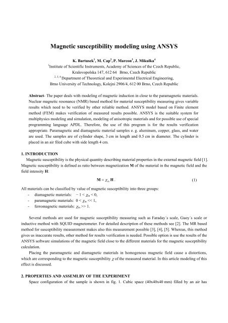
Magnetic susceptibility modeling using ANSYSK. Bartusek 1 , M. Cap 2 , P. Marcon 3 , J. Mikulka 41 Institute of Scientific Instruments, Academy of Sciences of the Czech Republic,Kralovopolska 147, 612 64 Brno, Czech Republic2, 3, 4Department of Theoretical and Experimental Electrical Engineering,Brno University of Technology, Kolejni 2906/4, 612 00 Brno, Czech RepublicAbstract- The paper deals with modeling of magnetic induction in close to the paramagnetic materials.Nuclear magnetic resonance (NMR) based method for material susceptibility measuring gives variableresults which need to be verified by other reliable method. ANSYS model based on Finite elementmethod (FEM) makes verification of measured results possible. ANSYS is the suitable system formultiphysics modeling and simulation, modeling of anisotropic materials and for possible use of specialprogramming language APDL. Therefore, the use of this program is for the results verificationappropriate. Paramagnetic and diamagnetic material samples e. g. aluminum, copper, glass, and waterare used. The samples are of cylinder shape, 3 cm in length and 0.5 cm in diameter. The cylinder isplaced in an air filed cube with side length 4 cm.1. INTRODUCTIONMagnetic susceptibility is the physical quantity describing material properties in the external magnetic field [1].Magnetic susceptibility is defined as ratio between magnetization M of the material in the magnetic field and thefield intensity H:M = χ mH. (1)All materials can be classified by value of magnetic susceptibility into three groups:- diamagnetic materials: − 1 < χ m < 0,- paramagnetic materials: 0 < χ m > 1.Several methods are used for magnetic susceptibility measuring such as Faraday´s scale, Guoy´s scale orinductive method with SQUID magnetometer. For detailed description of these methods see [2]. The MR basedmethod for susceptibility measurement makes also this measurement possible [3], [4], [5]. Whereas, this methodgives us inaccurate results, other method for results verification is needed. Possible option is use the results of theANSYS software simulations of the magnetic field close to the different materials for the magnetic susceptibilitycalculation.Placing the paramagnetic and diamagnetic materials in homogenous magnetic field cause a distortions,which are corresponding to the magnetic susceptibility χ of the measured material. In this article modeling of thiseffect is discussed.2. PROPERTIES AND ASSEMLBY OF THE EXPERIMENTSpace configuration of the sample is shown in fig. 1. Cubic space (40x40x40 mm) filled by an air has

magnetic susceptibility χ m1 = 0, labeled by number 1 in fig. 1. In the center of this space is placed the sample ofmentioned materials with different magnetic susceptibility χ m . The samples are cylindrical, 3 cm in length and0.5 cm in diameter, labeled by number 2 in fig. 1. There were used the paramagnetic aluminum sample (χ mAl =2.2·10 -5 ), the diamagnetic samples copper (χ mCu = -9.2·10 -6 ) and water (χ mAl = 2.2·10 -5 ). Section plane is placed tothe center of the cubic space, labeled by number 3 in fig. 1.1B2xz3Fig. 1: Configuration of the modeled system, cube filled by an air with sample.The model according to arrangement shown in fig. 1 was designed in ANSYS environment. The model wasdesigned by using of the finite element method with using of Solid 96 elements [6]. The boundary conditions werechosen according to the formula for the magnetic potential in order to value of a homogenous static magnetic fieldinduction was B = 4.7 T.φ B⋅z4.7 T ⋅40mm± = = . (2)2 2μ2μ0 03. NUMERICAL MODELINGANSYS is the suitable system for multiphysics modeling and simulation, anisotropic materials and forpossible use of special programming language APDL. ANSYS numerical analysis is based on Finite elementmethod. For describing of the quasi-stable model by the Finite element method are used the reduced Maxwell’sequations:rot H=J, divB =0, (3), (4)where H is the magnetic field intensity vector, B is the magnetic field induction vector, J is the current densityvector. For case of the irrotational field is the equation (3) in the form:Material relations are given by equation:rot H = 0 . (5)B= μ0μrH . (6)

4. RESULTS OF NUMERICAL MODELINGThe modeled magnetic induction in the section plane is shown in fig. 2. Value ΔB is deviation from the staticmagnetic field B 0 = 4.7 T. As a sample was used the aluminum sample and because of the paramagnetic propertiesis the magnetic field in the sample space magnified.Fig. 2: The behaviour of magnetic induction in the ax of the aluminum sample.Computed ΔB curve is used in the magnetic susceptibility equation:Bs − Bmχm= . (7)B 0Value Bs and B m represent the stabile value of B in space of the sample and the minimal B value just next tothe material sample. By using ΔB values from fig. 2 and equation (7) the magnetic susceptibility of aluminum hasbeen calculated to: χ cAl = 2.19·10 -5 . When we substitute the value of magnetic flux from fig. 3 to equation (7),Fig. 3: The behaviour of magnetic induction in the ax of the copper sample.

we obtain the calculated value of susceptibility of copper: χ cCu = 9.16·10 -6 . With values of the magnetic fluxfrom fig. 4 we obtain the calculated susceptibility for water: χ cH2O = 8.96·10 -6 .Fig. 4: The behaviour of magnetic induction in the ax of the water sample.Results on section planes in the ANSYS models are shown in fig. 5. On the left the red color in the space ofthe aluminum sample shows the local increment of the magnetic field and the blue color the static magnetic fieldB 0 . On the right is the local decrement (blue area) of the magnetic field in the place of the diamagnetic materialsample (copper, water). The red area corresponds to static magnetic field.-0,104E-4 0,142E-5 0.388E-4 0.635E-4-0,420E-4 -0,317E-4 -0.214E-4 -0.111E-40,190E-5 0,265E-4 0.512E-4 0.758E-4-0,368E-4 -0,265E-4 -0.162E-4 -0.595E-5Fig. 5: Slice through the center of the modeled system.5. CONCLUSIONSThe ANSYS environment was used for modeling of interactions of the magnetic field with paramagnetic anddiamagnetic samples. Proposed equation (7) gives values of the magnetic susceptibility with sufficient accuracy.

Higher level of the accuracy is possible with increasing of the element size. In table 1 is shown an overview of theactual values of magnetic susceptibility χ of measured materials and absolute errors Δχ calculated from the modelof individual samples.Tab. 1: Errors between the actual value of the magnetic susceptibility χ and the calculated value of Δχ.Samples χ [ppm] Δχ [ppm]copper -9.2 0.04water -9.0 0.04aluminum 2.2 -0.10It is possible to verify the experimental results of the magnetic susceptibility measuring for different materialsamples by modeling of the magnetic. This is important for example in MR methods.ACKNOWLEDGEMENTThe research described in the paper was financially supported by research plan No. MSM 0021630513, No.MSM 0021630516, grant of Czech ministry of industry and trade no. FR-TI1/001, Czech Science Foundation(102/09/0314) and project of the BUT Grant Agency FEKT-S-10-13.REFERENCES1. Dedek, L, Dedkova, J. Elektromagnetismus. 2. Brno: VUTIUM, 2000. 232 p. ISBN 80-214-1548-7.2. Steinbauer, M. Mereni magneticke susceptibility technikami tomografie magneticke resonance. VUT v Brne,FEKT, Brno 2006.3. Vladingerbroek, M. T., Den Boer, J. A. 1999. Magnetic resonance imaging. Heidelberg (Germany):Springer-Verlag, 1999. ISBN 3-540-64877-1.4. BARTUSEK, K., DOKOUPIL, Z., GESCHEIDTOVA, E. Mapping of magnetic field around small coils usingthe magnetic resonance method. Measurement Science and Technology, 2007, 18, p. 2223 - 2230.5. BARTUSEK, K., DOKOUPIL, Z., GESCHEIDTOVA, E. Magnetic field mapping around metal implantsusing an asymmetric spin-echo MRI sequence. Measurement Science and Technology, 17, No. 12, p. 3293.6. Fiala, P. Finite Element Method Analysis of a Magnetic Field Inside a Microwave Pulsed Generator, 2ndEuropean Symposium on Non-Lethal Weapons, May 13-15, 2003, Ettlingen, SRN.