Motor Control with Arduino: - ICC Media GmbH

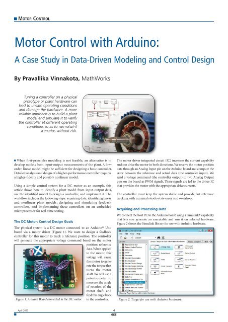
MOTOR CONTROLMotor Control with Arduino:A Case Study in Data-Driven Modeling and Control DesignBy Pravallika Vinnakota, MathWorksTuning a controller on a physicalprototype or plant hardware canlead to unsafe operating conditionsand damage the hardware. A morereliable approach is to build a plantmodel and simulate it to verifythe controller at different operatingconditions so as to run what-ifscenarios without risk. When first-principles modeling is not feasible, an alternative is todevelop models from input-output measurements of the plant. A loworder,linear model might be sufficient for designing a basic controller.Detailed analysis and design of a higher-performance controller requiresa higher-fidelity and possibly nonlinear model.Using a simple control system for a DC motor as an example, thisarticle shows how to identify a plant model from input-output data,use the identified model to design a controller, and implement it. Theworkflow includes the following steps: acquiring data, identifying linearand nonlinear plant models, designing and simulating feedbackcontrollers, and implementing these controllers on an embeddedmicroprocessor for real-time testing.The DC Motor: Control Design GoalsThe physical system is a DC motor connected to an Arduino® Unoboard via a motor driver (Figure 1). We want to design a feedbackcontroller for this motor to track a reference position. The controllerwill generate the appropriate voltage command based on the motorposition referencedata. When appliedto the motor, thisvoltage will causethe motor to generatethe torque thatturns the motorshaft. We will use apotentiometer tomeasure the angleof rotation of themotor shaft, andfeed this angle backto the controller.Figure 1. Arduino Board connected to the DC motor.The motor driver integrated circuit (IC) increases the current capabilityand can drive the motor in both directions. We receive the motor positiondata through an Analog Input pin on the Arduino board and compute theerror between the reference and actual data (the controller input). Wesend a voltage command (the controller output) to two Analog Outputpins on the board as PWM signals. These signals are fed to the driver ICthat provides the motor with the appropriate drive currents.The controller must keep the system stable and provide fast referencetracking with minimal steady-state error and overshoot.Acquiring and Processing DataWe connect the host PC to the Arduino board using a Simulink® capabilitythat lets you generate an executable and run it on selected hardware.Figure 2 shows the Simulink library for use with Arduino hardware.Figure 2. Target for use with Arduino hardware.April 2013 4

MOTOR CONTROLTo collect the data, the Arduino board will send voltage commands tothe motor and measure the resulting motor angles. We create a Simulinkmodel to enable data collection. The host machine must communicatewith the Arduino board to send voltage commands and receive back theangle data. We create a second model to enable this communication.In the model that will run on the Arduino Uno board (Figure 3), theMATLAB® Function block Voltage Command To Pins reads from theserial port and routes the voltage commands to the appropriate pins.We use serial communication protocol to enable the host computer tocommunicate with the Arduino board. In the CreateMessage subsystem,a complete serial message is generated from the motor position dataobtained from one of the analog input pins on the board.>> u = logsout.getElement(1).Values.Data;>> y = logsout.getElement(2).Values.Data;>> bounds1 =iddata(y,u,0.01,'InputName','Voltage','OutputName','Angle',......'InputUnit','V','OutputUnit','deg')Time domain data set with 1001 samples.Sample time: 0.01 secondsOutputs Unit (if specified)Angle degInputs Unit (if specified)Voltage VWe will be working with 12 data sets. These data sets were selected toensure adequate excitation of the system and to provide sufficient datafor model validation.Developing Plant Models from Experimental DataDeveloping plant models using system identification techniques involvesa tradeoff between model fidelity and modeling effort. The moreaccurate the model, the higher the cost in terms of effort and computationaltime. The goal is to find the simplest model that will adequatelycapture the dynamics of the system.Figure 3. Simulink model that will run on the Arduino board.We create a real-time application from the model by selecting Tools > Runon Target Hardware > Run. We are then ready to acquire the input/outputdata using the model that will run on the host computer (Figure 4).Figure 4. Model that will run on the host machine..We send various voltage profiles to excite the system, and record andlog the corresponding position data. At the end of the simulation, thesignal logging feature in Simulink will create a Simulink data set objectin the workspace containing all the logged signals as time-series objects.Next, we prepare the collected data for estimation and validation.Using the following commands, we convert the data into iddata objectsfor import into the System Identification Tool in System IdentificationToolbox.>> logsoutlogsout =Simulink.SimulationData.DatasetPackage: Simulink.SimulationDataCharacteristics:Name: 'logsout'Total Elements: 2Elements:1: 'Voltage'2: 'Angle'-Use getElement to access elements by index or name.-Use addElement or setElement to add or modify elements.Methods, SuperclassesWe follow the typical workflow for system identification: We start byestimating a simple linear system and then estimate a more detailednonlinear model that is a more accurate representation of the motorand captures the nonlinear behavior. While a linear model mightsuffice for most controller design applications, a nonlinear modelenables more accurate simulations of the system behavior and controllerdesign over a range of operating points.Linear System IdentificationUsing the iddata objects, we first estimate a linear dynamic model forthe plant as a continuous-time transfer function. For this estimation,we specify the number of poles and zeros. System Identification Toolboxthen automatically determines their locations to maximize the fit to theselected data sets.We launch the System Identification Tool by executing>> identWe can import the data sets into the tool from the base workspaceusing the Import Data pull-down menu (Figure 5). We also have theoption to preprocess the imported data. To start the estimation process,we select the working data that will be used to estimate a model and thevalidation data against which the estimated model will be tested. Wecan use the same data set for both estimation and validation initially,and then use other data sets to confirm our results. Figure 5 shows theSystem Identification Tool with the data set imported. The estimationdata set, data set 11, comes from an experiment designed to avoidexciting nonlinearities in the system.Figure 5. The System identification Tool with data imported.5 April 2013

MOTOR CONTROLNonlinear System IdentificationFigure 6. Continuous Transfer Functionestimation GUI.Figure 7. Plot comparing estimated modelresponse and estimation data.Figure 8. Plot comparing estimated modelresponse with validation data.We can now estimate acontinuoustransferfunction for this data.In our example, we estimatea 2-pole, no-zero,continuous-time transferfunction (Figure 6).We compare the simulationresponse of theestimatedmodelagainst measured databy checking the ModelOutput box in the SystemIdentification Tool.The fit between the responseof the estimatedlinear model and theestimation data is93.62% (Figure 7).To ensure that the estimatedtransfer functionrepresents themotor dynamics, wemust validate it againstan independent dataset. For this purposewe select data set 12,where the motor operateslinearly as our validationdata. We achievea reasonably accuratefit (Figure 8).While the fit is not perfect, the transfer function that we identified doesa good job of capturing the dynamics of the system. We can use thistransfer function to design a controller for the system.We can also analyze the effect of plant uncertainty. Models obtained withSystem Identification Toolbox contain information not only about the nominalparameter values but also about parameter uncertainty encapsulatedby the parameter covariance matrix. A measure of the reliability of themodel, the computed uncertainty is influenced by external disturbancesaffecting the system, unmodeleddynamics, andthe amount of collecteddata. We can visualizethe uncertainty by plottingits effect on themodel’s response. Forexample, we can generatethe Bode plot ofthe estimated transferfunction showing 1standard deviation confidencebound aroundFigure 9. Bode plot of the estimated modelshowing model uncertainty.the nominal response(Figure 9).A linear model of the motor dynamics, created by using data collectedfrom a linear region of its operation, is useful for designing an effectivecontroller. However, this plant model cannot capture nonlinear behaviorexhibited by the motor. For example, data set 2 shows that the motor’s responsesaturates at about 100°, and data set 3 shows that the motor is notresponsive to small command voltages, perhaps owing to dry friction.In this step, we will create a higher-fidelity model of the DC motor. Todo that, we estimate a nonlinear model for the DC motor. A closer inspectionof the data reveals that the change in the slope of the responseis not linearly related to the change in voltage. This trend suggests nonlinear,hysteresis-like behavior. Nonlinear ARX (NLARX) models offerconsiderable flexibility, enabling us to capture such behavior using arich set of nonlinear functions, such as wavelets and sigmoid networks.Furthermore, these models let us incorporate what we have discoveredabout the system nonlinearities using custom regressors.For the NLARX modeling to be effective, we need data that is rich in informationabout the nonlinearities. We merge three data sets to createthe estimation data. We merge five other data sets to create a larger,multi-experiment, validation data set.>> mergedD = merge(z7,z3,z6)Time domain data set containing 3 experiments.Experiment Samples Sample TimeExp1 5480 0.01Exp2 980 0.01Exp3 980 0.01OutputsAngleUnit (if specified)degInputs Unit (if specified)Voltage V>> mergedV = merge(z1,z2,z4,z5,z8);The nonlinear model had various adjustable components. We adjustedthe model orders, delays, type of nonlinear function, and the numberof units in the nonlinear function. We added regressors that representsaturation and dead-zone behavior. After several iterations, we chose amodel structure that employed a sigmoid network with a parallel linearfunction and used a subset of regressors as its inputs. The parametersof this model were estimated to achieve the best possible simulationresults (Figure 10).Figure 10. Nonlinear ARX model estimation GUI.The resulting model has an excellent fit of >90% for the estimationdata as well as for the validation data. This model can be used for controllerdesign as well as for analysis and prediction.April 2013 6

MOTOR CONTROLDesigning the ControllerWe are now ready to design a PID controller for the higher-fidelity nonlinearmodel. We linearize the estimated nonlinear model at an operatingpoint of interest and then design a controller for this linearized model.Testing the Controller on HardwareWe create a Simulink model with the controller and place it on the ArduinoUno board using Simulink built-in support for deploying modelsto target hardware (Figure 14).We tune the PID controller and then select its parameters (Figure 11).Figure 14. Model with the controller implemented on theArduino board. The subsystem Get Angle receives the referencesignal from the serial port and converts it to the desiredangle of the motor. The DC Motor subsystem configures theArduino board to interface with the physical motor.We designed a controller by linearizing the estimated nonlinear ARX modelabout a certain operating point. The results for this controller show that thehardware response is quite close to the simulation results (Figure 15).Figure 11. PID Tuner interface.We also check how this controller performs on the nonlinear model.Figure 12 shows the Simulink model that we use to obtain the simulationresponse of the nonlinear ARX model.Figure 12. Simulink model for testing the controller on the estimatednonlinear model.We then compare the linearized and nonlinear model closed-loop stepresponses for a desired reference position of 60° (Figure 13).Figure 13. Step response plot comparing simulation responses of nonlinearand linearized models.Figure 15. Plot comparing simulation and hardware responsesto a step reference for a controller designed using a linearizedmodel.We also tested how well the controller tracks a random reference command.We see that the hardware tracking performance is also very closeto that obtained during simulation (Figure 16).Figure 16. Plot comparing tracking performance insimulation and on hardware for the controllerdesigned using an estimated nonlinear model.This example,whilesimple,capturestheessentialstepsfor data-drivencontrol. We collectedinput/outputdata from agiven hardwaretarget and usedSystem IdentificationToolboxto construct modelsof the system.We showedhow you can create models of lower and higher fidelity and design controllersusing these estimated models. We then verified the performanceof our controllers on the actual hardware.7 April 2013