E-book NEW! - Congress.cimne.com
E-book NEW! - Congress.cimne.com
E-book NEW! - Congress.cimne.com
- No tags were found...

Create successful ePaper yourself
Turn your PDF publications into a flip-book with our unique Google optimized e-Paper software.
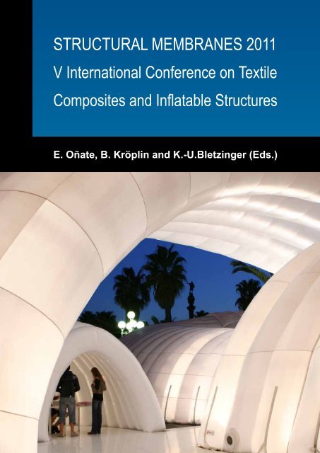
STRUCTURAL MEMBRANES 2011V International Conference on TextileComposites and Inflatable StructuresE. Oñate, B. Kröplin and K.-U.Bletzinger (Eds.)
Textile Composites and Inflatable Structures VStructural Membranes 2011
Textile Composites and Inflatable Structures VVolume containing the full length papers accepted for presentation at the V International Conference on TextileComposites and Inflatable Structures, Barcelona, Spain5-7 October 2011Edited by:E. OñateInternational Center for Numerical Methods in Engineering(CIMNE) and Universitat Politècnica de Catalunya, SpainB. KröplinTAO GmbH, GermanyK.-U. BletzingerTechnical University of Munich, GermanyA publication of:International Center for NumericalMethods in Engineering (CIMNE)Barcelona, Spain
International Center for Numerical Methods in Engineering (CIMNE)Gran Capitán s/n, 08034 Barcelona, Spainwww.<strong>cimne</strong>.<strong>com</strong>Textile Composites and Inflatable Structures IVE. Oñate, B. Kröplin and K.-U. Bletzinger (Eds.)First edition, December 2011© The authorsPrinted by: Artes Gráficas Torres S.L., Huelva 9, 08940 Cornellà de Llobregat, SpainDepósito legal: B-42318-2011ISBN: 978-84-89925-58-8
SUMMARYPreface .......................................................................................................................................... 7Acknowledgements ...................................................................................................................... 9Contents........................................................................................................................................11Plenary Lectures......................................................................................................................... 15Invited SessionsComputational Methods for Analysis of Tensile Structures.....................................................67Invited Session Organized by K.-U. Bletzinger, F. Dieringer and R. WüchnerDesign and Analysis of Inflatable Structures..........................................................................147Invited Session Organized by E. J. Barbero and B. N. BridgensDetailing - Case Studies - Installation Process.......................................................................221Invited Session Organized by J.I. LlorensEnvironment and Membranes...................................................................................................283Invited Session Organized by R. WagnerFluid-Structure Interaction and Wind Engineering.................................................................340Invited Session Organized by R. Wüchner and K.-U. BletzingerMembrane Mould........................................................................................................................397Invited Session Organized by A. PronkContributed SessionsAdaptivity and Applications .....................................................................................................456Design Methods .........................................................................................................................501Disaster Protection and Experimental Testing........................................................................555Numerical Methods for Structural Analysis.............................................................................563Testing and Maintenance ..........................................................................................................636Authors Index ............................................................................................................................6695
PREFACEThis volume contains the full length papers accepted for presentation at the V International Conference on TextileComposites and Inflatable Structures – Structural Membranes 2011, held in Barcelona, October 5-7, 2011. Previouseditions of the conference were held in Barcelona (2003), Stuttgart (2005), Barcelona (2007) and Stuttgart (2009).Structural Membranes is one of the Thematic Conference of the European Community in Computational Methods inApplied Science (ECCOMAS www.<strong>cimne</strong>.<strong>com</strong>/ec<strong>com</strong>as/) and is also a Special Interest Conference of the InternationalAssociation for Computational Mechanics (IACM http://www.<strong>cimne</strong>.<strong>com</strong>/iacm/).Textile <strong>com</strong>posites and inflatable structures have be<strong>com</strong>e increasingly popular for a variety of applications in – amongmany other fields - civil engineering, architecture and aerospace engineering. Typical examples include membrane roofsand covers, sails, inflatable buildings and pavilions, airships, inflatable furniture, airspace structures etc.The objectives of Structural Membranes 2011 are to collect and disseminate state-of-the-art research and technologyfor design, analysis, construction and maintenance of textile and inflatable structures.The ability to provide numerical simulations for increasingly <strong>com</strong>plex membrane and inflatable structures is advancingrapidly due to both remarkable strides in <strong>com</strong>puter hardware development and the improved maturity of <strong>com</strong>putationalprocedures for nonlinear structural systems. Significant progress has been made in the formulation of finite elementsmethods for static and dynamic problems, <strong>com</strong>plex constitutive material behaviour, coupled aero-elastic analysis etc.Structural Membranes 2011 addresses both the theoretical bases for structural analysis and the numerical algorithmsnecessary for efficient and robust <strong>com</strong>puter implementation.A significant part of the conference presents advances in new textile <strong>com</strong>posites for applications in membrane andinflatable structures, as well as in innovative design, construction and maintenance procedures.The collection of papers includes contributions sent directly from the authors and the editors cannot accept responsibilityfor any inaccuracies, <strong>com</strong>ments and opinions contained in the text.The organizers would like to take this opportunity to thank all authors for submitting their contributions.Barcelona, October 2011Eugenio OñateTechnical University of Catalunya(UPC) Barcelona, SpainBernd KröplinTao GmbH Stuttgart, GermanyKai-Uwe BletzingerTechnical University of Munich(TUM) Munich, Germany7
ACKNOWLEDGEMENTSThe conference organizers acknowledge the support towards the organization of the STRUCTURAL MEMBRANES2011 Conference to the following organizations:European Community on ComputationalMethods in Applied Sciences (ECCOMAS)International Association for Computational Mechanics (IACM)International Association for Shell and Spatial Structures (IASS)International Center for Numerical Methods in Engineering(CIMNE), SpainUniversitat Politécnica de Catalunya, SpainBuild Air Ingenieria y Arquitectura S.A.TAO GmbH, Stuttgart, Germany9
CONTENTSPLENARY LECTURESZoomorphism and Bio-Architecture: Between the Formal Analogy and the Application of Nature’s Principles.............17J.I. Llorens85 Ways to Make a Membrane Mould...........................................................................................................................28A. Pronk and M.M.T. DominicusSpace–Time FSI Modeling of Ringsail Parachute Clusters ..........................................................................................55K. Takizawa, T. Spielman and T. E. TezduyarINVITED SESSIONSComputational Methods for Analysis of Tensile StructuresInvited Session Organized by K.-U. Bletzinger, F. Dieringer and R. WüchnerPressurized Membranes for Structural Use: Interaction between Local Effects and Global Response........................67R. Barsotti and S.S. LigaròAir Volume Elements for Distribution of Pressure in Air Cushion Membranes..............................................................77J. BellmannAdvanced Cutting Pattern Generation – Consideration of Structural Requirements in the Optimization Process........84F. Dieringer, R. Wüchner and K.-U. BletzingerA Rotation Free Shell Triangle with Embedded Stiffeners.............................................................................................92F. Flores and E. OñateShape Analysis for Inflatable Structures with Water Pressure by the Simultaneus Control........................................104Z. M.Nizam, H. Obiya and K. IjimaFinite Element Analysis on Multi-chamber Tensairity-like Structures Filled with Fluid and/or Gas..............................115A. Maurer, A. Konyukhov and K. SchweizerhofDirect Area Minimization through Dynamic Relaxation...............................................................................................126R.M. Pauletti and D.M. GuirardiFinding Minimal and Non-Minimal Surfaces through the Natural Force Density Method............................................138R.M. PaulettiDesign and Analysis of Inflatable StructuresInvited Session Organized by E. J. Barbero and B. N. BridgensEnergy Saving Design of Membrane Building Envelopes...........................................................................................147J. CremersNumerical Investigation of the Structural Behaviour of a Deployable Tensairity Beam...............................................158L. De Laet, M. Mollaert, J. Roekens and R. H. LuchsingerShear Deformations in Inflated Cylindrical Beams: an old Model Revisited................................................................166S.S. Ligarò and R. BarsottiDesign Tools for Inflatable Structures..........................................................................................................................176R. Maffei, R. H. Luchsinger and A. ZanelliSimulation of Inflatable Structures: Two proposals of Dynamic Relaxation Methods usablewith any Type of Membrane Elements and any Reversible Behavior.........................................................................188J. Rodriguez, G. Rio, J.M. Cadou and J. Troufflard11
Preliminary Investigation of Tensairity Arches.............................................................................................................198J. Roekens, M. Mollaert, L. De Laet and R. H. LuchsingerShear and Bending Stiffnesses of Orthotropic Inflatable Tubes..................................................................................210J. C. ThomasDetailing - Case Studies - Installation ProcessInvited Session Organized by J.I. LlorensRecent Applications of Fabric Structures in Venezuela...............................................................................................221J. Leon and C.H. HernandezThe Design and Application of Lanterns in Tent Structures.........................................................................................233J.G. Oliva-Salinas and E. Valdez-OlmedoTensegrity Ring for a Sports Arena, Formfinding & Testing.........................................................................................244D. Peña, J.I. Llorens, R. Sastre, D. Crespo and J. MartínezShade Design in Spain: how to Protect against Heat and UV Radiation....................................................................252H. PoppinghausUsing Mobile Devices in Textile Architecture Design (iPad/iPhone)............................................................................262J. SanchezExperimental Manufacture of a Pneumatic Cushion made of ETFE Foils and OPV Cells..........................................271A. Zanelli, C. Monticelli, P. Beccarelli and H. Mohamed IbrahimEnvironment and MembranesInvited Session Organized by R. WagnerLightweight Photovoltaics............................................................................................................................................283T. FerwagnerTextile Membranes for Case of Emergency Flood Protection.....................................................................................293K. Heinlein and R. WagnerNumerical Investigations for an Alternative Textile Inverter Building in the Area of Solar Power Generation..............299K. Janssen-Tapken, A. Kneer, K. Reimann, E. Martens and T. KotitschkeMembrane Structures with Improved Thermal Properties...........................................................................................312M. KarwathDevelopment and Testing of Water-Filled Tube Systems for Flood Protection Measures...........................................319B. Koppe and B. BrinkmannA Simulation Model for the Yearly Energy Demand of Buildings with Two-or-More-Layered Textile Roofs.................330K. Reimann, A. Kneer, C. Weißhuhn and R. BlumFLUID-STRUCTURE INTERACTION AND WIND ENGINEERINGInvited Session Organized by R. Wüchner and K.-U. BletzingerInvestigation of an Elastoflexible Morphing Wing Configuration.................................................................................340B. Béguin, C. Breitsamter and N. AdamsPressure -Volume Coupling in Inflatable Structures....................................................................................................352M. Coelho, K.-U. Bletzinger and D. RoehlNumerical Tools for the Analysis of Parachutes..........................................................................................................364R. Flores, E. Ortega and E. OñateOn the Hydraulic and Structural Design of Fluid and Gas Filled Inflatable Dams to Control Water Flow in Rivers....374M. Gebhardt, A. Maurer and K. Schweizerhof12
Multiscale Sequentially-Coupled FSI Computation in Parachute Modeling................................................................385K. Takizawa, S. Wright, J. Christopher and T. E. TezduyarMEMBRANE MOULDInvited Session Organized by A. PronkStructural Dynamic Façade.........................................................................................................................................397A. HabrakenConcrete Shell Structures Revisited: Introducing a New ‘Low-Tech‘ Construction MethodUsing VACUUMATICS Formwork................................................................................................................................409F. Huijben, F. van Herwijnen and R. NijsseThe Use of Fabrics as Formwork for Concrete Structures and Elements...................................................................421R. PedreschiDevelopment and Evaluation of Mould for Double Curved Concrete Elements .........................................................432C. Raun, M. Kristensen and P.H. KirkegaardFabric-formed Concrete Member Design....................................................................................................................444R. SchmitzContributed SessionsADAPTIVITY AND APPLICATIONSDatabase Interactive and Analysis of the Pneumatic Envelope Systems, through the Studyof their Main Qualitative Parameters...........................................................................................................................456A. Gómez-González, J. Neila González and J. Monjo CarrióGeometry and Stiffness in the Case of Arch Supported Tensile Roofs with Block and Tackle Suspension................464K. HinczA Very Large Deployable Space Antenna Structure Based on Pantograph Tensioned Membranes...........................476T. Kuhn, H. Langer, S. Apenberg, B. Wei and L. Datashvili(Un)folding the Membrane in the Deployable Demonstrator of Contex-T...................................................................484M. Mollaert, L. De Laet, J. Roekens and N. De TemmermanLightweight and Transparent Covers...........................................................................................................................495I. Salvador Pinto and B. MorrisDESIGN METHODSMembrane Restrained Columns..................................................................................................................................501H. Alpermann and C. GengnagelSOFT.SPACES _ New Strategies for Membrane Architecture....................................................................................511G. FilzDirect Minimization Approaches on Static Problems of Membranes...........................................................................525M. Miki and K. KawaguchiReframing Textiles into Architectural Systems; Construction of a Membrane Shell by Patchwork..............................537I. Vrouwe, M. Feijen, R. Houtman and A. BorgartStep by Step Cost Estimation Tool for Form-active Structures....................................................................................549R. Wehdorn-Roithmayr and M. GiraldoDISASTER PROTECTION AND EXPERIMENTAL TESTINGImprovement of the System of Modular Inflated Shells by Means of Physical Modelling ..........................................555R. Tarczewski and B. Bober13
NUMERICAL METHODS FOR STRUCTURAL ANALYSISHomogenization and Modeling of Fiber Structured Materials.....................................................................................563S. Fillep and P. SteinmannA New Double Curved Element for Technical Textile Analysis with Bending Resistance............................................572D. HegyiEvaluation of the Structural Behavior of Textile Covers Subjected to Variations in Weather Conditions....................581C.H. HernandezAn Orthotropic Membrane Model Replaced with Line-members and the Large Deformation Analysis.......................592K. Ijima, H. Obiya and K. KidoForm-finding of Extensive Tensegrity using Truss Elements and Axial Force Lines....................................................603A. Matsuo, H. Obiya, K. Ijima and Z. M.NizamAnalysis of Thermal Evolution in Textile Fabrics using Advanced Microstructure Simulation Techniques..................614M. Roemmelt, A. August, B. Nestler and A. KneerMechanics of Local Buckling in Wrapping Fold Membrane.........................................................................................627Y. Satou and H. FuruyaTESTING AND MAINTENANCEDetermination of the Response of Coated Fabrics under Biaxial Stress: Comparison betweenDifferent Test Procedures............................................................................................................................................636C. Galliot and R. H. LuchsingerEffects on Elastic Constants of Technical Membranes Applying the Evaluation Methods of MSAJ/M-02-1995..........648J. Uhlemann, N. Stranghöner, H. Schmidt and K. SaxeIssues with Management, Maintenance and Upkeep in ETFE Enclosures.................................................................660J. Ward, J. Chilton and L. RowellAuthors Index ...........................................................................................................................................................66914
PLENARY LECTURES15
Zoomorphism and Bio-Architecture: Between the Formal Analogy and the Application of Nature’s Principles© 17
85 Ways to Make a Membrane Mould85 WAYS TO MAKE A MEMBRANE MOULDARNO D. C. PRONK*AND MAURICE M. T. DOMINICUS †Eindhoven University of TechnologyDepartment of Architecture Building and PlanningP.O. Box 513,Vertigo 7.14 5600 MB Eindhoven The Netherlands.e-mail: A.D.C.Pronk@tue.nl and M.M.T.Dominicus@tue.nlweb page: www.ArnoPronk.<strong>com</strong>Key words: Membranes, morphology, membrane moulds, fabric formwork, form finding, manipulation andadaption.Summary. The focus of this paper is on the form and materialization of membrane moulding. There hasbeen an impressive and long tradition in research on geometry and form finding of membranes. The use ofmembranes for moulding has been a growing in the last 10 years. However, if designers ask for the do’s anddon’ts in membrane moulding it is hard to give a clear and simple answer. This paper provides an overviewof all the possibilities for the manipulation of membranes. The overview is presented in a matrix with 85icons that represent 85 ways to manipulate a membrane. Further a general overview of the techniques andmethods for the use of membrane moulds will be given. Case studies by the author and others for the use ofglass, ice, concrete and <strong>com</strong>posite will be shown within this overview. The overviews in the paper aim to bea helpful instrument for designers who like to work with membrane moulds. For researchers in membranemoulding the overviews can be helpful to clarify which kind of <strong>com</strong>binations have been researched andwhich kind of <strong>com</strong>binations are still open for further research. In the future new techniques, materials and<strong>com</strong>binations can be added to the matrixes.1 INTRODUCTIONAlthough the title uses the term “membrane”, we prefer to use the term “form-active”. Form-active isused in the way defined by H. Engel: “Form-active structure systems are systems of flexible, non-rigidmatter, in which the redirection of forces is effected by a self-found Form design and characteristic Formstabilisation”. In practice form-active and flexible structures are pre-stressed membranes, inflatablemembranes, chains and cable structures. It is possible to use this type of structures for moulding. They havea double-curved surface and have the ability to make non-repetitive surfaces. This way of moulding is preeminentlysuitable for “free”-formed architecture and all kinds of doubly curved building elements.In this paper we will consequently connect colors to a certain form. The most important colors are:• yellow for zeroclastic;• green for monoclastic;• blue for synclastic; and• red for anticlastic.Figure 1 zeroclastic, monoclastic, synclastic and anticlasticsurfaces28
1.1 Pre-stressed membranesPre-stressed membranes are always anticlastic except forstructures having all the corner points in the same plane and all the forces on and in the structure are withinthe surface of that plane; in that case the form is zeroclastic. Using elastic fabrics the surface of the model isformed within a number of high-points, low-points and borders. The surfaces are not absolutely minimal.The geometry of the plane is determined by the extent to which the fabric is tensioned in one or moredirections. The degree of tension in the different directions can be changed and will influence the surface ofthe membrane. If the ratio of tension in the different directions is more than 1:2, depending on the materialproperties the membrane might wrinkle.1.2 Inflatable membranesInflatable membrane structures contain at least one direction, a circular cross section.In most cases, they are synclastic (Figure 2). Under certain conditions, it is also possible to containmonoclastic (Figure 3) and even anticlastic (Figure 4) surfaces. The different surfaces that can be made withinflatables depend on the circular cross section in relation to other circular cross sections. The twoparameters that influence the form are:1 the angle of the cross section to the other cross section; and2 the radius of the circle.Both parameters 1 and 2 can be divided into three subgroups:1a one centre point;1b parallel circular sections perpendicular to a straight center line; and1c non-parallel circular sections perpendicular to a central curvature.2a fixed radius;2b linear changing radius; and2c non-linear changing radius.Figure 2 Synclastic balloonFigure 3: MonoclasticballoonFigure 4: Balloon with ananticlastic partParameters 1 en 2 are <strong>com</strong>bined in Table 1 below and will lead to 7 ways to curve the surface of aninflatable. The table gives an examples of every category.Table 129
Below and in the tables there are drawings of inflatable objects with a particular curved surface.Figure:A, B, CFigure D, E, F1, F2Figure G1, G2Object A with one center is always a sphere. Spheres have a synclastic surface. Objects with one centerpoint in <strong>com</strong>bination with a changing radius do not exist. Object B and D with a parallel circular sectionon a straight line have always a monoclastic surface. Objects C and E have a synclastic and anticlasticpart following the curved centerline. At the “inner site” of the center curve the surface is anticlastic; at the“outer side” the surface is synclastic. Object F has a non-linear changing radius. If the radius changes in aprogressive way, the surface is anticlastic. If the radius changes in a regressive way, the surface is synclastic.Object G is a <strong>com</strong>bination of a curved center line and a non-linear changing radius. Both features willgive a double curvature. They can stimulate or de-stimulate each other. They stimulate each other in the<strong>com</strong>bination of outer side of the center curve and regressive curvature to a synclastic surface. In the case ofthe inner site of the center curve and progressive changing radius they stimulate each other to an anticlasticsurface. In the other two <strong>com</strong>binations (inner site of the curve – regressive changing radius and outer side ofthe curve and progressive changing radius) the feature with the strongest surface curvature will determinethe result. Below a scheme with the features and curvatures. The color of the scheme is corresponding to thecolor of the inflatable object below. The green arrow in object G shows the place where a synclastic surfaceswaps to and anticlastic surface as a result of the strong curvature of the center line although the change ofthe radius is repressive. The purple arrow in object G shows the place where an anticlastic surface swaps tosynclastic surface as a result of the strong curvature of the center line, although the change of the radius isprogressive.Table 230
Figure G3, G42 FORM FINDING2.1 Physical form findingLike every design process the form finding of tensile structures is an iterative process, i.e. the conditions canbe changed over and over until the most optimal solution is achieved. Finding a final solution is an interplaybetween the decisions taken by the designer and the form findings process. The form findings process that isused, might affect the results. Table 3 <strong>com</strong>pares two experimental form finding methods.BoundarySoap filmflexible or rigid closedElastic membrane/filmflexible or rigid points andMinimal surfaceboundariesabsolute minimal surfaceflexible or rigid boundariesdiffer from the minimalsurfaceForm anticlastic/ synclastic Anticlastic/synclasticSurface manipulation a) depends on the boundary a) depends on the boundaryconditionsb) pressure on the surfacec) material behaviourconditionsb) pressure on the surfacec) material behaviourd) depends on the direction andforce of the pretension in themembrane.Table 3: Comparison between physical methods: soap film versus elastic membrane/film31
2.2 Analytical form finding of membrane structuresUntil the 70ties of the last century physical form finding was used for engineering tensile structures. Theimplementation of the model has to be done as precise as possible. It is a time consuming process with therisk of many inaccuracies. After the knowledge gained during the construction of the Olympic Stadiumin Munich (1972) <strong>com</strong>puter programs were introduced for the engineering and form finding of membranestructures.In 1974, H.J. Schek published the paper “The force density method for form-finding and <strong>com</strong>putations ofgeneral networks”, the fundamental theory for the analytical approach of form finding, the force densitymethod. The <strong>com</strong>puter program Easy and, more recently, other programs use this method for form findingmembrane structures. In the analytical form findings process, according to Klaus Linkwitz, two phases canbe identified.2.2.1 Phase1A number of design studies, non-materialized equilibrium models, have to be done. The process is almostanalogous to the soap film method. Within the boundaries a minimal surface will be generated. Themembrane can be seen as the discretization of a cable net. There are a number of parameters that influencethe geometry of the equilibrium surface. By varying these parameters the geometry (curvature) of thesurface can be influenced. The parameters are:a) the position of boundaries, the high points and low points;b) the curvature of the surface;c) proportional force density in the different parts of the surface;d) orientation of the network; ande) external forces/load cases.In the first phase the equilibrium geometry of the surface is found. In this phase it is possible to dopreliminary studies to load cases, deformation, and stress contribution.2.2.2 Phase 2The second phase consists of the materialization of the equilibrium surface. By introduction of the materialproperties it is possible to have a <strong>com</strong>plete analysis of the load cases, deformation and stress contribution.The geometry of the surface will be influenced by the material properties.Phase 1 Phase 2conditions closed boundaries and/or points equilibrium (Phase 1)shape equilibrium materialised equilibriumshape influence a) boundaries, high points, low material propertiespointsb) the curvature of the surfacec) proportional force densityd) orientation of the networke) external forces/load casesTable 4: Process for the analytical form finding of membrane structures2.2.3 Dynamic relaxationIn the force density method there is a ratio between the force and the length of a line. This is specified bythe designer. Beside the force density method it is possible to calculate the deformation of membranes withthe dynamic relaxation method. The dynamic relaxation method is based on discretizing the continuumunder consideration by lumping the mass at nodes and defining the relationship between nodes in terms32
of stiffness. The system oscillates about the equilibrium position under the influence of loads. An iterativeprocess is followed by simulating a pseudo-dynamic process in time, with each iteration based on an updateof the geometry.3 THE MANIPULATION OF MEMBRANESThe surface of a membrane can be manipulated in different ways. This paragraph will give an overview ofthe different ways a membrane can be influenced.3.1 85 <strong>com</strong>binations to manipulate membranesIf single-layered form active surfaces in force equilibrium are brought in relation to their Gaussiancurvature, the following five <strong>com</strong>binations can be made:1. prestressed membrane or cable structure with an anticlastic surface;2. prestressed membrane or cable structure with a zeroclastic surface;3. inflatable with a synclastic surface;4. inflatable with a monoclastic surface; and5. inflatable with an anticlastic surface.The surfaces in force equilibrium can be manipulated in four different main categories:1. by changing the pre-stress in a certain area of the structure in force equilibrium;2. by an external load on the structure in force equilibrium;3. by pushing other surfaces in force equilibrium against a surface in force equilibrium; and4. by pushing a rigid element in or out the structure in force equilibrium.It is possible to <strong>com</strong>bine those different ways. In the scheme are 85 ways to manipulate membranes, it leadsto an endless number of forms that can be made, for instance the <strong>com</strong>bination of an inflatable pushed againsta pre-stressed membrane. Those membranes will still be in force equilibrium (from active). If a membraneis <strong>com</strong>bined with section active, vector active or surface active elements the amount of possibilities doesincrease further. In this way it is not possible to make every shape you can think of, but it is possible to <strong>com</strong>eclose to any shape desired. It is impossible to describe all the surfaces that can be made, but it is possible togive an overview of the different parameters for the manipulation of membranes.Below is the matrix with all the 85 possibilities. In column 1 to 5, the 5 types of membranes are given. Inthe rows the ways to manipulate are written divided into the 4 main categories as mentioned above. Pleasenote the legend for the meaning of the colors and marks. The manipulation will increase or decrease thecurvature. Not every <strong>com</strong>bination will give a manipulation with a 3D effect on the surface and some ofthe <strong>com</strong>binations will give the same result. For instance pushing or pulling against a zeroclastic membranewill give the same deformation if the result is mirrored in the plane of the membrane. There are 5 x 19<strong>com</strong>binations, taking out the <strong>com</strong>binations without a result or with the same result 85 <strong>com</strong>binations are left.33
Figure 5: scheme with 85 ways to manipulate membranes divided into 4 main categories.Below a closer look to the manipulation of membranes divided into the four main categories.34
3.2 Changing the pre-stress in a certain area of the structure in force equilibriumFigure 6: The effect of local pre-stressed areas.3.2.1 The experimtents by LinkwitzIn the specification of the force density in the field and in the boundaries it is possible to influence thegeometry of the equilibrium of the membrane. Linkwitz and a group of students did some experimentalresearch to the ratio of the force density and the geometry of the equilibrium. In this research theexperiments by Linkwitz have been redone in the program Tess3D.35
Figure 7,8. The influence of the size of the force density on the equilibrium shape.Fig. 4 shows a perpendicular net structure with a force density in the boundary of 1. In Fig. 5 the forcedensity in the boundary and the network is 5. The equilibrium shape of the surface is the same. Theconclusion is that if the ratio in force density of the boundary and the network is the same, the shape of thestructure will also be the same.Figure 9: The force density in the borders is 3 times bigger than in the network. Figure 10: The force density in theborder is 10 times bigger than in the network.The forces in the boundary are proportionately bigger than in the network. Therefore the curvature ofthe boundary is smaller and the surface of the network increases. Conclusion: if the force density in theboundary <strong>com</strong>pared to the network is bigger, the network will be<strong>com</strong>e bigger and the curvature in thenetwork and boundary will be<strong>com</strong>e smaller.Figure 11: The force density in the boundary is 3 times smaller than in the network. Figure 12: The density in theboundary is 6 times smaller than in the network.The force density in the network is relatively big <strong>com</strong>pared to the boundary cables. The curvature of the36
oundary cables is lower and the surface of the network is smaller. The above figures show that the shapeof the equilibrium depends on the proportional relationship between the force densities in boundaries andnetwork.3.2.2 The behavior of membranes.The work of Frei Otto and his team is of importance in a more experimental way to understand the rules forthe manipulation of membranes. For a better understanding please see the reference to the work publishedby F. Otto S. Pellegrino, B. Maurin, K.U. Bletzinger and R. Wagner.3.2.3 Local pre-stressed areas in anticlastic surfacesFigure 13 and 14: Two equilibrium surfaces with equal force density proportions in cable (1) and net (1). The forcedensity in the cable in figure 14 is 0. In Figure 15 the force density is 5.Figure 15, 16, 17, 18 and 19 Anticlastic membranes with a change in local pre-stressed areasIn case of a change in a local pre-stressed force within the surface, there will be a new state of forceequilibrium. Figure 15 shows a cable with a higher pre-stress. This cable can be seen as a new border. Figure10 shows that if the ratio between border and membrane be<strong>com</strong>es bigger the curvature be<strong>com</strong>es smaller andthe area be<strong>com</strong>es bigger. In Figure 14 and 15 is happening the same. The higher the stress in the cable theless curvature in membrane and cable. A pre-stressed cable on or in the surface of a mechanical pre-stressedmembrane will decrease the anticlastic curvature in the surface and will give a curved folding line at theposition of the cable.Figure 16 shows an area with a higher pre-stress. In that case the curvature perpendicular to the stress willincrease within that area. Outside the area and in the direction of the stress the curvature will decrease.Figure 17 shows a local area with pre-stress in both directions. In the part with the higer pre-stress thecurvature will increase in the other parts the curvature will decrease.Figure 18 and 19 shows a membrane with a local area with a relief of the pre-stress. In those parts willhappen the opposite of what happened in the membranes with a local higher pre-stress.In case the stress in a pre-stressed surface is locally lower in one direction, the curvature in that directionwill be higher but perpendicular the curvature in that area will be lower to the incensement of the curvaturein the surface beside this area;3.2.4 Local pre-stressed areas in zero clastic membranes37
Figure 20, Zero clastic membrane, Figure 21, 22, and 23 Inflatable membranes with a pre-stressed cableFigure 20 shows a zero clastic membrane. A higher pre-stress within the surface of the membrane will notlead to a curvature besides the wrinkling of the parts with a lower pre-stress. This will happen if the ratiobetween the tension in the both parts is more than 2.3.2.5 Inflatable membranes with a pre-stressed cableFigure 24, 25, and 26: Three equilibrium surfaces with the same equally spread upload. The force density proportionsin border cable, cross cable and net have been varied:• Figure 24 The force density in the border cable is 12, in the cross cable is 1 and net cable is 1• Figure 25 The force density in the border cable is 12, in the cross cable is 12 and net cable is 1• Figure 26 The force density in the border cable is 1, in the cross cable is 12 and net cable is 1Figure 21, 22 and 23 shows a pre-stressed cable on or in the surface of an inflatable. This will always givea synclastic curvature in the surface of the membrane. When the cable is pulled out of the surface of aninflatable, the surface next to the cable will be anticlastic.38
3.2.6 Inflatable membranes with a change in anisotropic pre-stressed areasFigure 27, Synclastic inflatable membrane with an anisotropic higher pre-stressed areaFigure 28, Monoclastic inflatable membrane with an anisotropic higher pre-stressed areaFigure 29 Anticlastic inflatable membrane with an anisotropic higher pre-stressed areaFigure 30, Synclastic inflatable membrane with an anisotropic lower pre-stressed areaFigure 31, Monoclastic inflatable membrane with an anisotropic lower pre-stressed areaFigure 32, Anticlastic inflatable membrane with an anisotropic higher pre-stressed areaIn case the stress in a pre-stressed or inflatable surface is locally higher in one direction, the curvature inthat direction will be lower but perpendicular, the curvature in that area will increase to the detriment of thecurvature in the surface beside this area.In case the stress in an inflatable with a synclastic surface is locally higher in one direction (Figure 27, 28and 29), the curvature in that direction will decrease. The surface in Figure 27 will be<strong>com</strong>e zeroclastic andthen even anticlastic. The surface in Figure 28 and 28 will be increasingly anticlastic.In Figure 30 and 31 the stress in an inflatable surface is locally lower in one direction, the synclasticcurvature in that direction will increase.In Figure 32 the stress in an inflatable with an anticlastic surface is locally lower in one direction, thecurvature in that direction will decrease to zeroclastic and then be<strong>com</strong>e synclastic.3.2.7 Inflatable membranes with a change in isotropic pre-stressed areasFigure 33, Synclastic inflatable membrane with an isotropic higher pre-stressed areaFigure 34, Monoclastic inflatable membrane with an isotropic higher pre-stressed areaFigure 35, Anticlastic inflatable membrane with an isotropic higher pre-stressed areaFigure 36, Synclastic inflatable membrane with an isotropic lower pre-stressed areaFigure 37, Monoclastic inflatable membrane with an isotropic lower pre-stressed areaFigure 38, Anticlastic inflatable membrane with an isotropic higher pre-stressed areaIn Figure 33, 34 and 35 the stress in a inflatable is locally higher in both directions, the curvature in that areawill increase to, or as, an anticlastic curvature. The inner pressure next to the higher stressed area will form asynclastic area.In Figure 36, 37 and 38 happens the opposite: the stress in a the inflatable is lower, the curvature in thatarea will increase to, or as, a synclastic surface. The surface area next to the lower stressed area will beanticlastic.39
3.3 External load on the structure in force equilibriumFigure 39: The effect of load cases40
3.3.1 Force density, curvature and deformationBelow some more experiments by Linkwitz and a group of students. In this research the experiments byLinkwitz have been redone in the program Tess3D. The influence of the force density on the deformation ofthe equilibrium surface as a result of a vertical point load is showed in Figure 40 and 41.Figure 40: The force in the boundary = 5, in the network = 1; on the network is a vertical point load with a size of 6.Figure 41: The force in the boundary = 5, in the network = 5; the vertical point load has a force equivalent of 6. Thefigures show that the higher the force density in the network, the smaller the deformation will be.The main curvature in the network will be influenced by the relative position of the points and theboundaries. There is a relation to the curvature of the network and the behaviour of the network under load:the lower the curvature, the smaller the deformation and vice versa.Figure 42 and 43: Two equilibrium surfaces with equal force density proportions and vertical point load but adifferent curvature.The experiments by Linkwitz show the possibilities to manipulate the form of pre-tensioned membranes andthe behaviour under load. Below some more experiments with the following <strong>com</strong>binations:1. an equally spread upload in <strong>com</strong>bination with one point load; and2. an equally spread upload in <strong>com</strong>bination with some cables.Figure 44, 45 and 46: Three equilibrium surfaces with an equally spread upload. The force density proportions inborder cable (12) and net (1) are equal. In figure 17 is the surface pulled down in one point with a force of 25. Infigure 18 is the surface pulled upwards in one point with a force of 19.41
3.3.2 Point loadFigure 47, Anticlastic membrane with a point loadFigure 48, Zeroclastic membrane with a point loadFigure 49, Synclastic inflatable membrane with a point loadFigure 50, monoclastic inflatable membrane with a point loadFigure 51, Anticlastic inflatable membrane with a point loadIn case of an external load, there will be a new state of force equilibrium. A pre-stressed surface in forceequilibrium will always make an anticlastic surface to the place of contact with another point.3.3.3 Linear load on a mechanical pre-stressed membraneFigure 52, Anticlastic membrane with a linear pushed loadFigure 53, Zeroclastic membrane with a linear pushed loadFigure 54, Anticlastic membrane with a linear pulled loadFigure 55, Zeroclastic membrane with a linear pulled loadFor anticlastic pre-stressed structures and zeroclastic surfaces the result for pulling and pushing is the same(Figure 52 and 54 as well as Figure 53 and 55). It will bring a curved line in the surface. The changedsurface will be anticlastic.42
3.3.5 Linear load on an inflatable membraneFigure 56, Synclastic inflatable membrane with a linear pushed loadFigure 57, Monoclastic inflatable membrane with a linear pushed loadFigure 58, Anticlastic inflatable membrane with a linear pushed loadFigure 59, Synclastic inflatable membrane with a linear pulled loadFigure 60, Monoclastic inflatable membrane with a linear pulled loadFigure 61, Anticlastic inflatable membrane with a linear pushed loadFor a linear load on an inflatable the result will bring a curved line in the surface of the membrane. Pushedfrom the outside (Figure 56, 57 and 58) the changed surface will be synclastic. Pulled from the outside(Figure 59, 60 and 61) the surface will be anticlastic.3.3.6 Local surface load mechanical pre-stressed membraneFigure 62, Anticlastic membrane with a local pushed surface loadFigure 63, Zeroclastic membrane with a local pushed surface loadFigure 64, Anticlastic membrane with a local pulled surface loadFigure 65, Zeroclastic membrane with a local pulled surface loadA surface load on an anticlastic surface will always decrease an anticlastic surface, if the force on the surfaceis strong enough, it will lead to a synclastic surface. A zeroclastic membrane will always form a synclasticsurface. For anticlastic pre-stressed structures and zeroclastic surfaces the result for pulling and pushing isthe same (Figure 62 and 64 as well as Figure 63 and 65).3.3.7 Load surface load inflatable membraneFigure 66, Synclastic membrane with a local pushed surface loadFigure 67, Zeroclastic membrane with a local pushed surface loadFigure 68, Anticlastic membrane with a local pushed surface loadFigure 69, Synclastic membrane with a local pulled surface loadFigure 70, Zeroclastic membrane with a local pulled surface loadFigure 71, Anticlastic membrane with a local pulled surface loadFigure 72 Sections of a synclastic membrane with a local pushed surface loadThe surface load on an inflatable will always end with a local synclastic surface if the force is strong enough.In Figure 68 and 71 the surface will decrease to zero clastic before it be<strong>com</strong>es anticlastic. In Figure 66 thesurface decreases to zero clastic and be<strong>com</strong>es synclastic in the opposite direction. At the borders of the“negative” synclastic surface to the “positive” curvature there will be a folding line or anticlastic area. See43
Figure 72.This is an overview with the results of the manipulation of membranes. For a better understanding of thebehavior of membranes with a variation in stress and load cases please see the referred papers by F. Otto S.Pellegrino, B. Maurin, K.U. Bletzinger and R. Wagner.3.4 Pushing surfaces in force equilibrium against another surface in force equilibriumFigure 73: The effect of pushed flexible elements44
Pushing surfaces in force equilibrium against another surface in force equilibrium will transform the twosurfaces in a new state of force equilibrium based on the forces and form of the two individual surfaces.Below the general rules:Figure 741. In the place of connection between both surfaces the angle between both surfaces is 0 as shown inFigure 74.2. If membrane structures are <strong>com</strong>bined, this will lead to a fluid surface to the place where bothsurfaces are connected.3. In the place of connection of the surfaces, the membrane with the highest tension demands the formof the surface.4. If the tension in both surfaces is the same, the surface will form a minimal surface within theboundaries of the connected area. That will be an anticlastic or zeroclastic surface;5. In all the cases where a membrane is pushed against a zeroclastic membrane (Figure 76, 86, 91 and96) the curvature of the membrane will be decreased.3.4.1 Pushing an anticlastic mechanical pre-stressed membrane against another membraneFigure 75, Anticlastic mechanical pre-stressed membrane pushed against another anticlastic mechanical pre-stressedmembraneFigure 76, Anticlastic mechanical pre-stressed membrane pushed against a zeroclastic mechanical pre -stressedmembraneFigure 77, Anticlastic mechanical pre-stressed membrane pushed against a synclastic inflatable membraneFigure 78, Anticlastic mechanical pre-stressed membrane pushed against a monoclastic inflatable membraneFigure 79, Anticlastic mechanical pre-stressed membrane pushed against an anticlastic inflatable membraneIn Figure 75 the connected area will be anticlastic. If the pre-stress in both membranes is the same the surfacewill form a minimal surface within the boundaries of the connected area.In Figure 78 and 79 the connected area will be anticlastic. If the pre-stress in both membranes is the same thesurface will differ from a minimal surface due to the overpressure at one side.In Figure 77 the connected area is anticlastic and decreses to zeroclastic to be<strong>com</strong>e synclastic if the tensionin the synclastic inflatable membrane and pushing force is strong enough.3.4.2 Pushing a zeroclastic pre-stressed membrane against another membraneFigure 80, Zeroclastic mechanical pre-stressed membrane pushed against an anticlastic mechanical pre-stressedmembraneFigure 81, Zeroclastic mechanical pre-stressed membrane pushed against another zeroclastic mechanical prestressedmembraneFigure 82, Zeroclastic mechanical pre-stressed membrane pushed against a synclastic inflatable membraneFigure 83, Zeroclastic mechanical pre-stressed membrane pushed against a monoclastic inflatable membraneFigure 84, Zeroclastic mechanical pre-stressed membrane pushed against an anticlastic inflatable membrane45
In all the figures the zeroclastic membrane will adapt the surface of the membrane pushed to. It will alsodecrease the curvature. In Figure 81 there is no manipulation.3.4.3 Pushing a synclastic inflatable against another membraneFigure 85, Synclastic inflatable membrane pushed against an anticlastic mechanical pre stressed membraneFigure 86, Synclastic inflatable membrane pushed against a zeroclastic mechanical pre stressed membraneFigure 87, Synclastic inflatable membrane pushed against another synclastic inflatable membraneFigure 88, Synclastic inflatable membrane pushed against a monoclastic inflatable membraneFigure 89, Synclastic inflatable membrane pushed against an anticlastic inflatable membraneIn Figure 87 the surface decreases to zeroclastic and be<strong>com</strong>es synclastic in the opposite direction. At theborders from the “negative” synclastic surface to the “positive” curvature there will be a folding line oranticlastic area (Figure 72).In Figures 85, 88 and 89 the surface decreases to zeroclastic and be<strong>com</strong>es anticlastic.3.4.4 Pushing a monoclastic inflatable against another membraneFigure 90, Monoclastic inflatable membrane pushed against an anticlastic mechanical pre-stressed membraneFigure 91, Monoclastic inflatable membrane pushed against a zeroclastic mechanical pre-stressed membraneFigure 92, Monoclastic inflatable membrane pushed against a synclastic inflatable membraneFigure 93, Monoclastic inflatable membrane pushed against another monoclastic inflatable membraneFigure 94, Monoclastic inflatable membrane pushed against an anticlastic inflatable membraneIn Figure 90 and 94 the surface decreases the anticlastic surface of the surface pushed in.In Figure 92 the curvature decreases to zeroclastic and be<strong>com</strong>es synclastic in the opposite direction. Atthe boundary of the “negative” synclastic surface to the “positive” curvature there will be a folding line oranticlastic area (Figure 72).In Figure 93 there are two cases: 1 the mono the surfaces have the same parallel direction. In that case themonoclastic curvatures decreases to zero clastic and be<strong>com</strong>es monoclastic in the opposite direction, at theboundary of the “negative” monoclastic surface to the “positive” curvature there will be a folding line ormonoclastic area. (Figure 72). In the other case the monoclastic surfaces are not parallel. In that case themonoclastic curvatures decreases to anticlastic and be<strong>com</strong>es monoclastic in the opposite direction, at theboundary of the “negative” monoclastic surface to the “positive” curvature there will be a folding line oranticlastic area.3.4.5 Pushing an anticlastic inflatable against another membrane46
Figure 95, Anticlastic inflatable membrane pushed against an anticlastic mechanical pre-stressed membraneFigure 96, Anticlastic inflatable membrane pushed against a zeroclastic mechanical pre-stressed membraneFigure 97, Anticlastic inflatable membrane pushed against a synclastic inflatable membraneFigure 98, Anticlastic inflatable membrane pushed against a monoclastic inflatable membraneFigure 99, Anticlastic inflatable membrane pushed against another anticlastic inflatable membraneIn Figure 99 the connected area will be anticlastic. If the pre-stress in both membranes is the same the surfacewill be a minimal surface.In Figure 95 and 98 the connected area will be anticlastic. If the pre-stress in both membranes is the same thesurface will differ from a minimal surface due to the overpressure at one side.In Figure 97 the connected area is anticlastic and decreases to zeroclastic to be<strong>com</strong>e synclastic if the tensionin the synclastic inflatable membrane and pushing force is strong enough.This is an overview with the results of the manipulation of membranes. For a better understanding of themechanical behavior of membranes in force equilibrium against another surface in force equilibrium pleaseread more about this in the referred papers.3.5 Pushing a rigid element into or out of a membrane structure in force equilibriumFigure 98: Pushing a rigid element into or out of a membrane structure in force equilibrium47
3.5.1 General rules for pushing rigid elementsGeneral rules for the surfaces in force equilibrium that will be manipulated by pushing a rigid element intoor out of the structure.1. if a rigid element is pushed against the surface in force equilibrium, the structure will adapt thesurface of the rigid element unless the boundaries/surface of the rigid element allow the flexiblesurface to form a new surface in force equilibrium released from the surface of the rigid element.This is shown below in Figure 99E;2. if there is contact between two surfaces, the angle between them is zero;3. if the angle between the surfaces fluently increases from zero, the release between the surfaces iswithin a place on the two surfaces. In that case there is a smooth transition between the two surfacesinto a joint surface. This is shown below in Figure 99A, 99C and F;4. if the angle between the surfaces changes suddenly, the release between the surfaces is at one of theboundaries of the surface. This will give a (curved) line within the other flexible surface. This isshown below in Figure 99B and 99D and 99E.A B C D E FFigure 99: The section of a surface in force equilibrium pushed against a rigid element.3.5.2 Pushed-out elements from the inside of an inflatableFigure 100, Synclastic inflatable membrane with a pushed-out elementFigure 101, Monoclastic inflatable membrane with a pushed-out elementFigure 102, Anticlastic inflatable membrane with a pushed-out elementAn inflatable structure will make an anticlastic surface to the boarders of any rigid element pushed out fromthe inside.3.5.3 Pushed-in elements against mechanical prestressed membranesFigure 103, Anticlastic mechanical pre-stressed membrane with a pushed-in elementFigure 104, Zeroclastic mechanical pre-stressed membrane with a pushed in-elementFigure 105, Anticlastic mechanical pre-stressed membrane with a pushed-in element with a positive boundaryFigure 106, Zeroclastic mechanical pre-stressed membrane with a pushed-in element with a positive boundaryFigure 107, Anticlastic mechanical pre-stressed membrane with a pushed-in element with a negative boundaryFigure 108, Zeroclastic mechanical pre-stressed membrane with a pushed-in element with a negative boundaryA zeroclastic mechanical prestressed membrane and an anticlastic mechanical prestressed membrane willmake an anticlastic surface to the boundaries of any rigid element pushed-in or out as long as the boundariesare not parallel.48
3.5.4 Pushed-in elements with a parallel boundary curveFigure 109, Anticlastic mechanical pre-stressed membrane with a pushed-in element with parallel boundariesFigure 110, Zeroclastic mechanical pre-stressed membrane with a pushed-in element with parallel boundariesFigure 111, Monoclastic inflatable with a pushed-in element with parallel boundariesFigure 112, Anticlastic inflatable with a pushed-in element with parallel boundariesIf the boarders of a zeroclastic mechanical pre-stressed membrane and an anticlastic mechanical pre-stressedmembrane are parallel with the element pushed-in, it will form a zeroclastic surface.If the direction of a monoclastic or synclastic inflatable surface is parallel to a monoclastic or zeroclasticelement or straight boundary line the surface will be monoclastic.3.5.5 Pushed in elements with a positive boundary curve against an inflatableFigure 113, Synclastic inflatable membrane with a pushed-in element with a positive boundaryFigure 114, monoclastic inflatable membrane with a pushed-in element with a positive boundaryFigure 115, Anticlastic inflatable membrane with a pushed-in element with a positive boundaryAn inflatable structure will make an anticlastic surface to the boundary of any rigid element pushed-in fromthe outside with a positive boarder curvature, also if the positive boundary-line is parallel to the boundarylineof the membrane.3.5.6 Pushed-in elements with a negative boundary curve against an inflatableFigure 116, Synclastic inflatable membrane with a pushed-in element with a negative boundaryFigure 117, monoclastic inflatable membrane with a pushed-in element with a negative boundaryFigure 118, Anticlastic inflatable membrane with a pushed-in element with a negative boundaryAn inflatable structure will make a synclastic surface when a rigid element with a negatively curvedboundary is pushed in from the outside.49
4 Rigidizing membrane moulds.There are many types of form-active structures and many ways to make a rigid surface with the help ofa form-active structure. The diagram below will give an overview of all the possibilities known for thematerials: concrete, water, polymer <strong>com</strong>posites and glass. The possibilities are characterized in 6 differentaspects. This overview gives the opportunity to look for new <strong>com</strong>binations. The product and function of theproduct is in this overview of minor importance. In the last column case studies are mentioned. Of coursethis is not a final list. If new techniques will be developed the list can be extended and new <strong>com</strong>binations canbe made.1 The four materials to make the transition from fluid to solid are:• concrete• ice/water• polymer <strong>com</strong>posites• glass.2 The form-active structure: the structural typology of the form active structure• cable net• woven fabric• knitted fabric• textile <strong>com</strong>posite• foil• the material of the shell in “fluid” condition• hinged plate structure3 Form-active typology: Amount of layers and connection between the layers• single layer• double layer• connected double layer4 Way to stabilize the mould: How the from-active mould is stabilized• (pre-)stressed surface• inflate• bending stiffness of a material• hydraulic pressure• under pressure•5 Technique to handle the rigidizing material:• hand layup• spraying• vacuum injection• submersion• casting• pumping• prefab elements6 Reinforcement of the material:• non• single fibers• ropes/cables• bars• fabric (woven)• woven fabric50
7 Surface treatment:• non• surface tension of the material• plastering• polishing• coating• drape• melting• sprayingFigure 119, Diagram of materials and techniques for ridgidizing form-active structure, all the possibilities availablefor glass, <strong>com</strong>posite, ice and concreteFigure 119 gives an overview of all the technical possibilities. In the diagram below (Figure 120) are all thetechniques known in relation to the material glass. In the last-column case studies will be mentioned. Figure121, 122 and 123 will deal with the materials Ice, Composite and Concrete.4.1 GlassFigure 12, Glass and the techniques to make doubly curved surfaces with a form-active mould51
4.2 IceFigure 121 Ice and the techniques to make doubly curved surfaces with a form-active mould4.3 CompositeFigure 122 Composite and the techniques to make doubly curved surfaces with a form active mould4.4 Concrete52
Figure 123 Concrete and the techniques to make doubly curved surfaces with a form-active mould.5 ConclusionsEven well-trained researchers in the field of membranes have problems to predict the out<strong>com</strong>e of themanipulation of membranes. The aim of this paper is to give an overview of all the possibilities for themanipulation of membranes. The result is a matrix with 85 ways to manipulate a membrane. With thismatrix we like to give insight in the effect and possibilities in an early stage during the form-finding process.The technical possibilities for rigidizing are not further clarified in this paper. In the near future more papersabout the materials concrete, ice, polymer <strong>com</strong>posites and glass in relation to membrane moulding will bepublished. The overviews in the paper aim to be a helpful instrument for designers who like to work withmembrane moulds. For researchers in membrane moulding the overviews can be helpful to clarify what kindof <strong>com</strong>binations have been made and which kind of <strong>com</strong>binations are still open for further research. In thefuture new techniques, materials and <strong>com</strong>binations can be added to the matrixes. The author will publish thematrixes on internet and invites researchers and producers to add their work to the matrixes.7 AcknowledgmentsThe experiments in the diagrams above by the author took a period of 10 years. The authors gratefullyacknowledge the support of many students, college’s, funds, <strong>com</strong>panies and the generous and visionarypolicy of the Eindhoven University of Technology who gave the confidence to do so many experiments issuch a wide field.53
7.1 Reference:[1] K. Linkwitz and H-J Schek, Einige bemerkungen zur berechnung von vorgespannten seilnetzkonstuktionen,Ingenieur-archiv, 40: 145-158, 1971[2] H-J Schek, The force density method for form finding and <strong>com</strong>putation of general networks. Computermethods in applied mechanics and engineering, 3: 115-134, 1974[4] K. Linkwitz, Experience from a course on “formfinding and analysis of tension structures”, held at theuniversity of Stuttgart for 10 years, International journal of space structures, 17, 159-169 (2002).[5] K. Linkwitz, About formfinding of double-curved structures, Engineering structures, 21, 709-718 (1999)[6] M. Mollaert, Teaching tension structures, International journal of space structures, 17, 171-181 (2002)[7] A. Capasso, M. Majowiecki and V. Pinto, La tensostrutture a membrane per l’architettura, Maggiolieditore (1993)[12] R. Wagner, Kinematics in tensioned structures, Textile <strong>com</strong>posites and inflatable structures, II, 85-97,(2008)[14] R. Wagner, On the design process of tensile structures, Textile <strong>com</strong>posites and inflated structures, II, 1-16,(2005).[15] F. Otto, Form (form-kraft-masse 2) – ein vorschlag zur entwicklung einer method zur ordnung undbeschreibung von formen, IL Institut für leichte flächentragwerke, 22, 1988.[16] H. Isler, Creating models, Application of structural morphology to architecture, IASS working group“Structural morphology”, 221, (1994).[18] IL 33, Radiolaria, Institut für leichte flächentragwerke (IL), Universität Stuttgart, (1990)[19] IL 35, Pneu und knochen – pneu and bone, Institut für leichte flächentragwerke (IL), Universität Stuttgart,(1995)[20] IL 6, Biology and building, Institut für leichte flächentragwerke (IL), Universität Stuttgart, (1973)[21]IL 9, Pneus in natur und technik – pneus in nature and technics, Institut für leichte flächentragwerke (IL),Universität Stuttgart, (1976)[22] M. Emmer, Soap films and soap bubbles: from Plateau to the Olympic swimming pool in Beijing, Springerverlag,Mathknow, 120-129, (2009)[23] F.J. Almgren, Jr. Minimal surface forms, Mathematical Intelligencer, 4, 164-172, (1988)[25] H.Engel, Tragsysteme – Structure systems, Verlag Gerd Hatje, (1997).[26] IL17, The work of Frei Otto and his teams 1955-1976, Institut für leichte flächentragwerke (IL), UniversitätStuttgart, (1978)[27] IL 18, Seifenblasen – Forming bubbles, Institut für leichte flächentragwerke (IL), Universität Stuttgart,(1988)[28] H. Pottmann, A.Asperl, M. Hofer and A. Kilian, Architectural Geometry, Bentley Institute Press, (2007)[30] K.A. Seffen, Z.You and S. Pellegrino, Folding and deployment of curved tape springs, Internationaljournal of mechanical sciences, 42, 2055-2073, (2000)[32] M. Pagitz and S. Pellegrino, Buckling pressure of “pumpkin” balloons, International journal of solidsand structures, 44, 6963-6986, (2007).[33] M. Pagitz, Y. Xu and S. Pellegrino, Stability of lobed balloons, Advances in space research, 37, 2059-2069, (2006).[34] D.S. Wakefield, Engineering analysis of tension structures; theory and practice, Engineering structures,21, 680-690, (1999).[35] B. Maurin and R. Motro, The surface stress density method as a form-finding tool for tensile membranes,Engineering structures, 20, 712-719, (1998).[36] K.U. Bletzinger and E. Ramm, Structural optimization and form finding of light weight structures,Computers and structures, 79, 2053-2062, (2001).[37] A. Pronk, S.L. Veldman and R. Houtman, Making double curved forms with the use of a 3d fabric, (2001).54
Space–Time FSI Modeling of Ringsail Parachute ClustersInternational Conference on Textile Composites and Inflatable StructuresSTRUCTURAL MEMBRANES 2011E. Oñate, B. Kröplin and K.-U.Bletzinger (Eds)SPACE–TIME FSI MODELING OF RINGSAIL PARACHUTECLUSTERSKENJI TAKIZAWA ∗ , TIMOTHY SPIELMAN † AND TAYFUN E.TEZDUYAR †∗ Department of Modern Mechanical Engineering andWaseda Institute for Advanced Study, Waseda University1-6-1 Nishi-Waseda, Shinjuku-ku, Tokyo 169-8050, JAPAN† Mechanical Engineering, Rice University – MS 3216100 Main Street, Houston, TX 77005, USAKey words: Fluid–structure interaction, Parachute clusters, Ringsail parachute, Space–time technique, Geometric porosity, ContactAbstract. The <strong>com</strong>putational challenges posed by fluid–structure interaction (FSI) modelingof ringsail parachute clusters include the lightness of the membrane and cable structureof the canopy <strong>com</strong>pared to the air masses involved in the parachute dynamics, geometric<strong>com</strong>plexities created by the construction of the canopy from “rings” and “sails”with hundreds of ring gaps and sail slits, and the contact between the parachutes. TheTeam for Advanced Flow Simulation and Modeling (T⋆AFSM) has successfully addressedthese <strong>com</strong>putational challenges with the Stabilized Space–Time FSI technique (SSTFSI),which was developed and improved over the years by the T⋆AFSM and serves as thecore numerical technology, and a number of special techniques developed in conjunctionwith the SSTFSI. We present the results obtained with the FSI <strong>com</strong>putation of parachuteclusters and the related dynamical analysis.1 INTRODUCTIONFluid–structure interaction (FSI) modeling of ringsail parachute clusters poses a numberof <strong>com</strong>putational challenges. The membrane and cable structure of the canopy ismuch lighter <strong>com</strong>pared to the air masses involved in the parachute dynamics, and this requiresa robust FSI coupling technique. This challenge is of course not limited to ringsailparachutes but is <strong>com</strong>mon to all parachute FSI <strong>com</strong>putations. The geometric challengecreated by the construction of the canopy from “rings” and “sails” with hundreds of ringgaps and sail slits requires a <strong>com</strong>putational model that makes the problem tractable.Contact between the parachutes requires an algorithm that protects the fluid mechanics155
Kenji Takizawa, Timothy Spielman and Tayfun E. Tezduyarmesh from excessive deformation, and this <strong>com</strong>putational challenge might also be encounteredin other classes of FSI problems where two solid surfaces <strong>com</strong>e into contact. TheTeam for Advanced Flow Simulation and Modeling (T⋆AFSM) has successfully addressedthese <strong>com</strong>putational challenges with the Stabilized Space–Time FSI technique (SSTFSI),which was developed and improved over the years by the T⋆AFSM and serves as the corenumerical technology, and special techniques developed in conjunction with the SSTFSI.The SSTFSI technique was introduced in [1]. It is based on the new-generationDeforming-Spatial-Domain/Stabilized Space–Time (DSD/SST) formulations, which werealso introduced in [1], increasing the scope and performance of the DSD/SST formulationsdeveloped earlier [2, 3, 4, 5] for <strong>com</strong>putation of flows with moving boundaries andinterfaces, including FSI. This core technology was used in a large number of parachuteFSI <strong>com</strong>putations (see, for example, [1, 6, 7, 8, 9, 10, 11, 12]). The direct and quasi-directFSI coupling techniques, which are generalizations of the monolithic solution techniquesto cases with in<strong>com</strong>patible fluid and structure meshes at the interface, were introducedin [13]. They provide robustness even in <strong>com</strong>putations where the structure is light <strong>com</strong>paredto the fluid masses involved in the dynamics of the FSI problem and were also used ina large number of parachute FSI <strong>com</strong>putations (see, for example, [1, 6, 7, 8, 9, 10, 11, 12]).Computer modeling of large ringsail parachutes by the T⋆AFSM was first reportedin [6, 7]. The geometric challenge created by the ringsail construction was addressedwith the Homogenized Modeling of Geometric Porosity (HMGP) [6], adaptive HMGP [8]and a new version of the HMGP that is called “HMGP-FG” [9]. Additional special techniquesthe T⋆AFSM introduced in the context of ringsail parachutes include the FSIGeometric Smoothing Technique (FSI-GST) [1], Separated Stress Projection (SSP) [6],“symmetric FSI” technique [8], a method that accounts for the fluid forces acting on structural<strong>com</strong>ponents (such as parachute suspension lines) that are not expected to influencethe flow [8], and other interface projection techniques [14].The T⋆AFSM recently started addressing (see [10, 11]) the challenge created by thecontact between the parachutes. In a contact algorithm to be used in this context, theobjective is to prevent the structural surfaces from <strong>com</strong>ing closer than a predeterminedminimum distance we would like to maintain to protect the quality of the fluid mechanicsmesh between the structural surfaces. The Surface-Edge-Node Contact Tracking(SENCT) technique was introduced in [1] for this purpose. It had two versions: SENCT-Force (SENCT-F) and SENCT-Displacement (SENCT-D). In the SENCT-F technique,which is the relevant version here, the contacted node is subjected to penalty forces thatare inversely proportional to the projection distances to the contacting surfaces, edgesand nodes. For FSI problems with in<strong>com</strong>patible fluid and structure meshes at the interface,it was proposed in Remark 1 of [6] to formulate the contact model based on thefluid mechanics mesh at the interface. This version of the SENCT was denoted with theoption key “-M1”. The contact algorithm used in the parachute cluster <strong>com</strong>putationsreported in [10] has some features in <strong>com</strong>mon with the SENCT-F technique but is morerobust. Also, <strong>com</strong>pared to the SENCT-F technique, the forces are applied in a conserva-256
Kenji Takizawa, Timothy Spielman and Tayfun E. Tezduyartive fashion. We call the new technique “SENCT-FC”, where the letter “C” stands for“conservative”. The new technique was used with option M1 in [10]. The SENCT-FCtechnique was described in detail in [11] and was used with option M1 also in the cluster<strong>com</strong>putations reported in that article. This short article uses material from [11]. Wepresent the <strong>com</strong>putational results together with the related dynamical analysis.2 CLUSTER COMPUTATIONSA series of two-parachute cluster <strong>com</strong>putations were carried out in [11] to determinehow the parameters representing the payload models and starting conditions affect longtermcluster dynamics. The parachute clusters reported in [11] were used with a 19,200 lbpayload. Each parachute has 80 gores and 4 rings and 9 sails, with 4 ring gaps and 8sail slits. Figure 1 shows, for an inflated ringsail parachute from [9], the ring and sailconstruction and the ring gaps and sail slits. More information on the parachutes can beFigure 1: A four-gore slice of a ringsail parachute in its inflated form. The pictures on the right illustratethe ring and sail construction of the canopy and show the shapes of the ring gaps and sail slits.found in [7, 8, 9]. The parameters selected for testing were the payload-model configurationsand initial coning angles (θ INIT ) and parachute diameters (D INIT ) (for readers notfamiliar with the term “coning angle”, see [11]). We also investigated two scenarios toapproximate the conditions immediately after parachute disreefing. This is explained inmore detail in a later paragraph. In all cases, the θ INIT is the same for both parachutesThe first set of <strong>com</strong>putations were carried out to investigate the effect of the payloadmodel. In drop tests, the parachutes are connected to a rectangular pallet that is weightedto represent the mass and inertial properties of a proposed crew capsule. The preliminaryparachute cluster <strong>com</strong>putations reported in [10] modeled the payload as a point masslocated at the confluence of the risers. We will refer to this as the payload at the confluence357
Kenji Takizawa, Timothy Spielman and Tayfun E. Tezduyar(PAC) configuration. Two new <strong>com</strong>putational payload models were created to see howthey would influence parachute behavior. The payload lower than the confluence (PLC)configuration adds another cable element below the confluence and models the payload asa point mass at the location of the pallet center of gravity. The payload as a truss element(PTE) configuration further enhances the model by distributing the payload mass at 9different points to match the mass, center of gravity, and six <strong>com</strong>ponents of the inertiatensor of the pallet. This is ac<strong>com</strong>plished by adding 5 cable elements and 26 truss elementsbelow the confluence. In all of the payload <strong>com</strong>parison <strong>com</strong>putations, θ INIT = 35 ◦ .The second set of <strong>com</strong>putations were carried out to investigate the effect of θ INIT . Threevalues of θ INIT were tested: 15 ◦ , 25 ◦ , and 35 ◦ . It should be noted that 35 ◦ is greater thanthe θ values seen in drop tests. The average θ during normal descent is around 15 ◦ , andthe maximum θ does not usually exceed 25 ◦ . We used θ INIT = 35 ◦ only to cause a largeperturbation in order to analyze the dynamic response of the parachute cluster. All ofthe θ INIT <strong>com</strong>parison <strong>com</strong>putations used the PTE configuration.The parachute described in [11] uses a reefing technique to permit incremental openingof the canopy. The parachute skirt is initially constricted by reefing lines and the reefinglines are cut at predetermined time intervals to allow the canopy to “disreef” to largerdiameters. In the third set of <strong>com</strong>putations, two scenarios were <strong>com</strong>puted to analyze howconditions immediately after disreefing could have an effect on long-term dynamics. Inthe first scenario, which we call “simulated disreef”, θ INIT = 10 ◦ , and for both parachutesD INIT = 70 ft. These values represent the approximate θ during final disreefing andthe average minimum D during nominal descent. The second scenario represents an“asynchronous disreef” by using for one parachute D INIT = 70 ft, and for the other D INIT= 90 ft. These values represent the average minimum and maximum parachute diametersduring nominal descent, respectively. Both scenarios used the PTE configuration.2.1 Starting conditionsBefore an FSI <strong>com</strong>putation is started, a series of pre-FSI <strong>com</strong>putations are carried outto build a good starting condition. For the process of building the starting condition, werefer the reader to [11].2.2 Computational conditionsFigure 2 shows, for a single parachute, the canopy structure mesh and the fluid mechanicsinterface mesh. The fluid mechanics mesh is cylindrical with a diameter of 1,740 ft anda height of 1,566 ft. It consists of four-node tetrahedral elements, while the fluid interfacemesh consists of three-node triangular elements. The number of nodes and elements aregiven in Table 1. The porosity model is HMGP-FG. The interface-stress projection isbased on the SSP. For more information on the <strong>com</strong>putational conditions, we refer thereader to [11]. We <strong>com</strong>puted each parachute cluster for a total of about 75 s, with remeshas needed to preserve mesh quality. The frequency of remeshing varies for each <strong>com</strong>pu-458
Kenji Takizawa, Timothy Spielman and Tayfun E. TezduyarFigure 2: Canopy structure mesh (left) and fluid mechanics interface mesh (right) for a single parachute.The structure has 30,722 nodes, 26,000 four-node quadrilateral membrane elements, and 12,521 two-nodecable elements. There are 29,200 nodes on the canopy. The fluid mechanics interface mesh has 2,140nodes and 4,180 three-node triangular elements.tation and usually depends on how often the parachutes collide, how much the clusterrotates about the vertical axis, and how much each parachute rotates about its own axis.Depending on the <strong>com</strong>putation, remeshing was needed every 170 to 370 time steps.2.3 ResultsFigures 3–6 show the descent speed U and the drag coefficient, which is calculated asC D = W/( 1ρU 2 S2 o ), where W is the payload weight, ρ is the density of the air, and S o isthe nominal area of the parachute.38.036.034.0PACPLCPTE1.31.21.11.0PACPLCPTEU (ft/s)32.030.028.0C D0.90.80.70.626.00 10 20 30 40 50 60 70 80Time (s)0.50 10 20 30 40 50 60 70 80Time (s)Figure 3: Cluster <strong>com</strong>putations for different payload models and θ INIT = 35 ◦ .559
Kenji Takizawa, Timothy Spielman and Tayfun E. TezduyarStructureFluidnn 61,443Membrane ne 52,000Cable ne 25,042Payload ne 1Interfacenn 58,400ne 52,000InterfaceVolume (15 ◦ , 80/80 ft)Volume (25 ◦ , 80/80 ft)Volume (35 ◦ , 80/80 ft)Volume (10 ◦ , 70/70 ft)Volume (35 ◦ , 70/90 ft)nn 4,280ne 8,360nn 197,288ne 1,210,349nn 280,601ne 1,739,739nn 289,679ne 1,797,003nn 352,861ne 2,199,472nn 289,221ne 1,795,542Table 1: Number of nodes and elements for the two-parachute clusters before any payload modifications.Here nn and ne are number of nodes and elements, respectively. The fluid mechanics volume meshis tabulated for different <strong>com</strong>binations of θ INIT and D INIT values. The PLC configuration has 1 morestructure node and 1 more cable element. The PTE configuration has 10 more structure nodes, 5 morecable elements, 26 more truss elements, and 8 more payload elements.Figures 7–8 show the contact between two parachutes from the asynchronous-disreef<strong>com</strong>putation. Figures 9–12 show the vent-separation distance (L VS ) for all cluster <strong>com</strong>putations.The horizontal black line on each plot shows the approximate vent-separationdistance when the parachutes are in contact. Tables 2–4 summarize the payload descentspeeds and drag coefficients for all of the cluster <strong>com</strong>putations.Payload Model U (ft/s) C DPAC 28.1 0.97PLC 30.1 0.85PTE 29.5 0.88Table 2: Average U and C D for different payload models with θ INIT = 35 ◦ . Statistical analysis begins20 s after the start of the <strong>com</strong>putation.3 CONCLUDING REMARKSWe have presented our FSI <strong>com</strong>putations of clusters of large ringsail parachutes, whichare constructed from membranes and cables with hundreds of ring gaps and sail slits. Thecore technology is the SSTFSI technique, supplemented with special FSI techniques. Many660
Kenji Takizawa, Timothy Spielman and Tayfun E. Tezduyar38.036.034.0θ INIT = 15°θ INIT = 25°θ INIT = 35°1.31.21.11.0θ INIT = 15°θ INIT = 25°θ INIT = 35°U (ft/s)32.030.028.0C D0.90.80.70.626.00 10 20 30 40 50 60 70 80Time (s)0.50 10 20 30 40 50 60 70 80Time (s)Figure 4:Cluster <strong>com</strong>putations for PTE and different θ INIT values.38.01.336.034.01.21.11.0U (ft/s)32.030.028.0C D0.90.80.70.626.00 10 20 30 40 50 60 70 80Time (s)0.50 10 20 30 40 50 60 70 80Time (s)Figure 5:Cluster <strong>com</strong>putations for simulated disreef.of the special techniques were developed to address the challenges involved in <strong>com</strong>putermodeling of ringsail parachutes. They include the homogenization techniques that makethe problem tractable despite hundreds of gaps and slits. Another special techniqueaddresses the <strong>com</strong>putational challenge created by the contact between the parachutes ofa cluster. We have also presented a dynamical analysis of the <strong>com</strong>puted results.ACKNOWLEDGMENTThis work was supported by NASA Grant NNX09AM89G, and also in part by the RiceComputational Research Cluster funded by NSF Grant CNS-0821727.REFERENCES[1] T.E. Tezduyar and S. Sathe, “Modeling of fluid–structure interactions with thespace–time finite elements: Solution techniques”, International Journal for NumericalMethods in Fluids, 54 (2007) 855–900, doi: 10.1002/fld.1430.761
Kenji Takizawa, Timothy Spielman and Tayfun E. Tezduyar38.01.336.034.01.21.11.0U (ft/s)32.030.028.0C D0.90.80.70.626.00 10 20 30 40 50 60 70 80Time (s)0.50 10 20 30 40 50 60 70 80Time (s)Figure 6:Cluster <strong>com</strong>putations for asynchronous disreef.θ INIT U (ft/s) C D15 ◦ 29.9 0.8625 ◦ 31.4 0.7835 ◦ 29.5 0.88Table 3: Average U and C D for PTE and different values of θ INIT . Statistical analysis begins 20 s afterthe start of the <strong>com</strong>putation.[2] T.E. Tezduyar, “Stabilized finite element formulations for in<strong>com</strong>pressible flow<strong>com</strong>putations”, Advances in Applied Mechanics, 28 (1992) 1–44, doi: 10.1016/S0065-2156(08)70153-4.[3] T.E. Tezduyar, M. Behr, and J. Liou, “A new strategy for finite element <strong>com</strong>putationsinvolving moving boundaries and interfaces – the deforming-spatial-domain/space–time procedure: I. The concept and the preliminary numerical tests”, ComputerMethods in Applied Mechanics and Engineering, 94 (1992) 339–351, doi: 10.1016/0045-7825(92)90059-S.[4] T.E. Tezduyar, M. Behr, S. Mittal, and J. Liou, “A new strategy for finite element<strong>com</strong>putations involving moving boundaries and interfaces – the deformingspatial-domain/space–timeprocedure: II. Computation of free-surface flows, two-U (ft/s) C DSimulated Disreef 30.6 0.82Asynchronous Disreef 30.8 0.81Table 4: Average U and C D for the disreef cases. Statistical analysis begins 5 s after the start ofthe <strong>com</strong>putation for the simulated-disreef case, and 20 s after the start of the <strong>com</strong>putation for theasynchronous-disreef case.862
Kenji Takizawa, Timothy Spielman and Tayfun E. TezduyarFigure 7: Parachutes at t = 52.20 s, t = 53.36 s and t = 54.52 s during the asynchronous-disreef<strong>com</strong>putation modeling the contact between parachutes.liquid flows, and flows with drifting cylinders”, Computer Methods in Applied Mechanicsand Engineering, 94 (1992) 353–371, doi: 10.1016/0045-7825(92)90060-W.[5] T.E. Tezduyar, “Computation of moving boundaries and interfaces and stabilizationparameters”, International Journal for Numerical Methods in Fluids, 43 (2003) 555–575, doi: 10.1002/fld.505.[6] T.E. Tezduyar, S. Sathe, J. Pausewang, M. Schwaab, J. Christopher, and J. Crabtree,“Interface projection techniques for fluid–structure interaction modeling withmoving-mesh methods”, Computational Mechanics, 43 (2008) 39–49, doi: 10.1007/s00466-008-0261-7.[7] T.E. Tezduyar, S. Sathe, J. Pausewang, M. Schwaab, J. Christopher, and J. Crabtree,“Fluid–structure interaction modeling of ringsail parachutes”, ComputationalMechanics, 43 (2008) 133–142, doi: 10.1007/s00466-008-0260-8.[8] T.E. Tezduyar, K. Takizawa, C. Moorman, S. Wright, and J. Christopher, “Space–time finite element <strong>com</strong>putation of <strong>com</strong>plex fluid–structure interactions”, InternationalJournal for Numerical Methods in Fluids, 64 (2010) 1201–1218, doi:10.1002/fld.2221.[9] K. Takizawa, C. Moorman, S. Wright, T. Spielman, and T.E. Tezduyar, “Fluid–structure interaction modeling and performance analysis of the Orion spacecraft963
Kenji Takizawa, Timothy Spielman and Tayfun E. TezduyarFigure 8: Parachutes at t = 55.68 s, t = 56.84 s and t = 58.00 s during the asynchronous-disreef<strong>com</strong>putation modeling the contact between parachutes.parachutes”, International Journal for Numerical Methods in Fluids, 65 (2011) 271–285, doi: 10.1002/fld.2348.[10] K. Takizawa, S. Wright, C. Moorman, and T.E. Tezduyar, “Fluid–structure interactionmodeling of parachute clusters”, International Journal for Numerical Methodsin Fluids, 65 (2011) 286–307, doi: 10.1002/fld.2359.[11] K. Takizawa, T. Spielman, and T.E. Tezduyar, “Space–time FSI modeling anddynamical analysis of spacecraft parachutes and parachute clusters”, ComputationalMechanics, published online, DOI: 10.1007/s00466-011-0590-9, April 2011, doi:10.1007/s00466-011-0590-9.[12] K. Takizawa, T. Spielman, C. Moorman, and T.E. Tezduyar, “Fluid–structure interactionmodeling of spacecraft parachutes for simulation-based design”, Journal ofApplied Mechanics, to appear, 2011.[13] T.E. Tezduyar, S. Sathe, R. Keedy, and K. Stein, “Space–time finite element techniquesfor <strong>com</strong>putation of fluid–structure interactions”, Computer Methods in AppliedMechanics and Engineering, 195 (2006) 2002–2027, doi: 10.1016/j.cma.2004.09.014.[14] K. Takizawa, C. Moorman, S. Wright, J. Christopher, and T.E. Tezduyar, “Wallshear stress calculations in space–time finite element <strong>com</strong>putation of arterial fluid–1064
Kenji Takizawa, Timothy Spielman and Tayfun E. Tezduyar300300250250200200L VS (ft)150L VS (ft)150100100505000 10 20 30 40 50 60 70 80Time (s)00 10 20 30 40 50 60 70 80Time (s)Figure 9: Vent-separation distance. Left: PAC and θ INIT = 35 ◦ , Right: PLC and θ INIT = 35 ◦ .300250200L VS (ft)1501005000 10 20 30 40 50 60 70 80Time (s)Figure 10: Vent-separation distance. PTE and θ INIT = 35 ◦ .structure interactions”, Computational Mechanics, 46 (2010) 31–41, doi: 10.1007/s00466-009-0425-0.1165
Kenji Takizawa, Timothy Spielman and Tayfun E. Tezduyar300300250250200200L VS (ft)150L VS (ft)150100100505000 10 20 30 40 50 60 70 80Time (s)00 10 20 30 40 50 60 70 80Time (s)Figure 11: Vent-separation distance. Left: PTE and θ INIT = 15 ◦ , Right: PTE and θ INIT = 25 ◦ .300.0300250.0250200.0200L VS (ft)150.0L VS (ft)150100.010050.0500.00 10 20 30 40 50 60 70 80Time (s)00 10 20 30 40 50 60 70 80Time (s)Figure 12:Vent-separation distance. Left: Simulated-disreef, Right: Asynchronous-disreef.1266
Pressurized Membranes for Structural Use: Interaction between Local Effects and Global ResponseInternational Conference on Textile Composites and Inflatable StructuresSTRUCTURAL MEMBRANES 2011E. Oñate, B. Kröplin and K.-U.Bletzinger (Eds)© CIMNE, Barcelona, 2011PRESSURIZED MEMBRANES FOR STRUCTURAL USE: INTERACTIONBETWEEN LOCAL EFFECTS AND GLOBAL RESPONSERICCARDO BARSOTTI * AND SALVATORE S. LIGARÒ †* Department of Civil EngineeringUniversity of PisaLargo L. Lazzarino, 1 56126 Pisa, Italye-mail: r.barsotti@ing.unipi.it† Department of Civil EngineeringUniversity of PisaLargo L. Lazzarino, 1 56126 Pisa, Italye-mail: s.ligaro@ing.unipi.itKey words: Inflatable beams, Wrinkling, Non-linear elastic behaviour.Summary. This paper is aimed to assess the non-linear elastic response of an inflatablecylindrical beam through a simple mechanical model recently proposed by the authors 1 tostudy the equilibrium shapes of highly pressurized elastic membranes. The local geometricnonlinearities due to the wrinkling of the membrane are taken into account by means of anequivalent physical non-linearity, assuming a two-states constitutive law for the material:when a fiber is stretched (the active state), its response is elastic, while when the fiber iscontracted, no <strong>com</strong>pressive force can be engendered in it (the passive state). The evolution ofthe wrinkled regions and the distribution of longitudinal and transverse stresses in themembrane are accurately determined for increasing levels of loads, up to the collapse. Thenumerical results, obtained through an expressly developed incremental-iterative algorithm,are then <strong>com</strong>pared with the experimental ones available in the literature.1 INTRODUCTIONIn recent years the number of applications where use has been made of textile structuresunder form of pressurized membranes has seen a steady growth in many areas of engineering.Compared to ordinary structures, inflatable ones are lighter and economic, are easily portable,and enable their rapid set up and final removal.Beams and arches, made of highly pressurized very flexible membranes, properlystrengthened by textile or glass fibers, are a viable alternative to more traditional choices in allthose cases in which the speed of execution or the lightness constitute primary requirements(consider, for example, all the emergency situations where shelters need to be erected as soonas possible, or the structures designed to operate in the space). However, some basic aspectscharacterizing the mechanical response of the inflatable elements have not yet entirely clearedand may therefore be placed among the current topics of mechanics of structures 2 .The equilibrium states of these elements are characterized by strong geometrical nonlinearities(local buckling and wrinkling phenomena) due to the smallness of membrane67
Riccardo Barsotti and Salvatore S. Ligaròthickness values, which may interest large portions of their surface. Moreover, with increasingloads, the size of the corrugated zones, whose position constitutes one of the main unknownsof the problem, tends to increase, thus strongly influencing the overall behaviour of the wholeelement and, what it is most important, its actual carrying capacity.In this paper we assess the state of stress in the wall of an inflatable cylindrical beamthrough a simple mechanical model recently proposed by the authors to study the equilibriumshapes of highly pressurized elastic membranes 1 . The aforesaid local geometric nonlinearitiesare taken into account by means of an equivalent physical non-linearity, assuming a twostatesconstitutive law for the material: when a fiber is stretched (the active state), its responseis elastic, while when the fiber is contracted, no <strong>com</strong>pressive force can be engendered in it(the passive state). The evolution of the corrugated regions and the distribution of longitudinaland transverse stresses in the membrane are determined accurately for increasing levels ofloads, up to the collapse. The numerical results, obtained by an expressly developedincremental-iterative algorithm, are then <strong>com</strong>pared with the numerical and experimental onesavailable in the literature 3, 4 .2 THE BENDING OF AN INFLATABLE BEAMIn the following, we will investigate the bending response of a cylindrical inflatable beam,variously supported at its ends, subjected to a transversal concentrated load 2F acting in themiddle section (Figure 1). The beam is made up of two rectangular elastic sheets of initiallength 2L and height h, joined together along their <strong>com</strong>mon boundaries.In all the cases examined the dimensions of the beam are kept fixed, as well as themechanical parameters of the material. The equilibrium problem will be solved for differentvalues of the pressure p and of the transversal load 2F for each of the two cases correspondingto simply-supported and built-in ends, respectively.2FhpFigure 1: the inflatable beam.The solutions will be obtained numerically by making use of an expressly developedincremental-iterative algorithm implemented in a FEM code, already proposed by the authors,which accounts for the local geometric nonlinearities resulting from the wrinkling of themembrane by means of an equivalent physical non-linearity.To improve the rate of convergence and the stability of the numerical algorithm, the loadprocess is subdivided into three separate phases. The membrane starts the load process in its2L268
Riccardo Barsotti and Salvatore S. Ligaròreference configuration where it is flat and unstressed. During the first phase, the pressure iskept equal to zero while a uniform antagonist plane traction is assumed to act along theboundary until a final value for it is reached. During the successive phase two, an increasingpressure p acts internally, up to its established final value. Finally, in the following phasethree the boundary traction progressively reduces to zero and wrinkling may freely develops.In all the three phases the analysis is performed by the same incremental-iterative procedurealthough the first pre-tensioning phase may be performed within a single load step.At the end of each incremental step, equilibrium is imposed via the virtual work principle.Large displacements and strains are considered, while a nonlinear elastic constitutive lawwhich makes uses of a relaxed energy is included into the analytical model to account forwrinkling.In all the numerical analyses the membrane material is assumed to behave as linear elasticunder tension with a Young’s modulus of E = 2.5 GPa and a Poisson’s ratio of ν = 0.3; themembrane thickness is set equal to 0.125 mm, the height and the length of the beam are setequal to 126 mm and 660 mm, respectively.2.1 A simply-supported beamThe first case taken under investigation is that of the simply-supported inflatable beamshowed in Figure 2. It is assumed that the beam, initially lying in the x-y plane, is first inflatedup to the final pressure p (accordingly, the central part of the beam be<strong>com</strong>es a cylinder ofradius approximately equal to R = 40 mm); then, it is subjected to the action of the load 2F.By virtue of symmetry, only one half of the beam has been modeled (Figure 3a).y2FhOpx2LFigure 2: the simply-supported inflatable beam.The inflated configuration together with three equilibrium configurations is showed inFigure 3. In the picture, wrinkled elements are represented in red colour, taut ones in bleu.After the beam is inflated some first wrinkled zones appear in correspondence to thesimply-supported end; in the following loading phase a second wrinkled region spreads itselfin the middle of the beam as the concentrated load increases. In the case where the internalpressure is kept fixed, the wrinkled region at the end of the inflated beam turns out to bealmost unaffected by the magnitude of the load F. The effects of end wrinkled regions,measured in terms of strains and stresses, are detectable only in the lateral parts of the beam 1369
Riccardo Barsotti and Salvatore S. Ligaròwhile the standard uniform tensile state of stress persists in the cylindrical central part of theinflated configuration (see Figure 3b).ha)L(Side view)(Shape of the cross-sectionin the middle of the beam)b)F=24.4 Nc)Figure 3: a) the FEM mesh; b) the inflated configuration; c) three equilibrium configurations corresponding toF =20.2 N, 26.0 N and 22.4 N respectively (left half of the beam; red elements are in a wrinkled state;p = 0.1 N/mm 2 , E = 2500 N/mm 2 , ν = 0.3, t = 0.125 mm)On the contrary, the extension of the wrinkled region under the point load increases with Fand the wrinkling produces effects which are not confined to a local scale but influence theload-displacement response of the inflated beam as a whole.470
Riccardo Barsotti and Salvatore S. LigaròFigure 4 shows the central part of the beam. A noteworthy mechanical phenomenonemerges from a closer observation of the evolution of the shape of the wrinkled region underthe point load. As one may easily verify, the spreading of wrinkles due to the <strong>com</strong>pressivestresses produced by the bending moment (which is maximum in the middle section) ishindered by an increase in the tensile stresses at the extrados of the beam due to the localpunching action of the concentrated load 2F.F = 20.2 N;v = 44 mmF = 26.0 N;v = 104 mmF = 22.4 N;v = 164 mma) b)Figure 4: wrinkled region in the middle of the beam for F =20.2 N, 26.0 N and 22.4 N.a) side view; b) axonometric view (p = 0.1 N/mm 2 , E = 2500 N/mm 2 , ν = 0.3, t = 0.125 mm).As a result, the wrinkled region is smaller than that which would be forecasted by means ofa one-dimensional beam model; consequently, the stiffness of the inflated beam in the threedimensionalmodel will be higher. Notwithstanding this, it is reasonable to think that the loaddisplacementresponse of the present 3d model would be in good agreement with that571
Riccardo Barsotti and Salvatore S. Ligaròobtained by a one-dimensional model (a confirmation of this may be found, for example, inreference 2 ). In fact, the increase in the stiffness due to the reduction of the wrinkled region isbalanced by an increase in the vertical displacements due to the local punching action of theforce 2F.To highlight this feature two load-displacement curves, one regarding the application pointof the load and the other the corresponding point on the axis of the inflatable beam, areshowed in Figure 5. Both are obtained by using the present three-dimensional model in thecase where the pressure p is kept fixed to the value of 0.1 N/mm 2 , the Young’s modulus andthe Poisson’s ratio of the membrane are set equal to E = 2,500 MPa and ν = 0.3, respectively,and the membrane thickness is assumed equal to t = 0.125 mm.In the same figure, a straight line starting from the origin and whose slope is the stiffness:324EπRtk el = ,3Lrepresents the response of a standard linear elastic beam. As it can be seen, this straight lineresults tangent to the load-displacement curve of the inflated beam (obviously, the oneregarding the displacement of the point of the line of axis in correspondence to the loadedpoint) within a good approximation. The tangent stiffness here obtained, equal to 0.66 N/mm,results quite close to that obtained numerically 3 (0.68 N/mm) for a cantilever inflated beamhaving half the span of the beam considered here and the same geometrical and mechanicalproperties.Figure 5: load-displacement curve for p = 0.1 N/mm 2 (E = 2500 N/mm 2 , ν = 0.3, t = 0.125 mm).It is worth observing that the differences between the two load-displacement curves ofFigure 5 increase linearly for low values of the load, i.e. when the central part of the inflatedbeam is slightly wrinkled only in proximity of the loaded point. The same difference resultsinstead to be quite constant when the load approaches its limit value and a spreading ofwrinkles in the central part of the inflated beam is observed. The increase in the verticaldisplacement due to the punching effect may also explain the <strong>com</strong>monly observed difference672
Riccardo Barsotti and Salvatore S. Ligaròbetween experimental and theoretical displacements 4 .Figure 6: principal stresses in the membrane for vertical displacement of the point of application of the loadequal to 164 mm (left half of the beam; p = 0.1 N/mm 2 , E = 2500 N/mm 2 , ν = 0.3, t = 0.125 mm).The stress distribution in the membrane obtained by the same non-linear FEM analysisconfirms the presence of the wrinkled region in the middle of the beam. Moreover, it provideswith useful hints about the magnitude of the transversal stresses and about the transmission ofthe shear force. As an example, the case illustrated in Figure 6 clearly shows that in thecentral part of the beam, where a wide wrinkled region is present, the circumferential tensilestresses are far from being uniform so the shear force is transmitted almost exclusively by theunwrinkled part of the cross-section.The stiffening effect produced by an increasing internal pressure is showed in Figure 7.Here, the load vs. pressure diagram is obtained by imposing to the loaded point a fixeddisplacement of 84 mm and by checking the magnitude of the load for increasing pressure.Two different responses are recognizable depending on whether the pressure is lower orhigher than a threshold value, which in the case examined turns out to be equal to about0.4 N/mm 2 . In the low pressure range (p < 0.4 N/mm 2 ), the central part of the beam is in awrinkled state and a small increase in the pressure results in a strong stiffening of the beam (tothis regard, in Figure 7 the dashed straight line representing the separation curve betweenwrinkled and unwrinkled responses of the beam is plotted). For higher pressures instead(p > 0.4 N/mm 2 ), the beam is unwrinkled and the stiffening effect is due to the decrease in the773
Riccardo Barsotti and Salvatore S. Ligaròdisplacements in the small punched region just under the load.WrinkledconfigurationsUnwrinkledconfigurations(vert. displ. 84 mm)Wrinkled beamUnwrinkled beam2.2 The built-in beamFigure 7: load vs. pressure diagram for vertical displacement of the loaded pointequal to 84 mm (p = 0.1 N/mm 2 , E = 2500 N/mm 2 , ν = 0.3, t = 0.125 mm).The second case taken under consideration is that of the built-in inflatable beam showed inFigure 8. It is assumed that the built-in constraint is first imposed to both the ends of thebeam, which initially lies in the x-y plane. Then the beam is inflated up to the final pressure p(accordingly, the central part of the beam be<strong>com</strong>es a cylinder of radius approximately equal toR = 40 mm) and finally the load 2F is applied. Once again, by virtue of symmetry, only onehalf of the beam has been modeled.y2FhOpx2LFigure 8: the built-in inflatable beam.The inflated configuration together with the loaded one corresponding to a verticaldisplacement of the loaded point equal to 100 mm is showed in Figure 9.874
Riccardo Barsotti and Salvatore S. Ligaròa)b)Figure 9: a) the inflated configuration; b) equilibrium configuration corresponding to F =192 N (left half of thebeam; red elements are in a wrinkled state; p = 0.1 N/mm 2 , E = 2500 N/mm 2 , ν = 0.3, t = 0.125 mm)Contrary to the simply-supported case examined in the preceding section, here a very smallincrease in the extension of the wrinkling regions (located under the point load and at thebuilt-in ends) is observed as the force F grows.a) b)Figure 10: load-displacement curve (a) and axial force-displacement curve (b) for p = 0.1 N/mm 2(E = 2500 N/mm 2 , ν = 0.3, t = 0.125 mm).The strongly different behaviour of the built-in beam is highlighted in the loaddisplacementdiagram showed in Figure 10a. The beam shows progressive stiffening as thevertical displacement of the loaded point increases and no softening phase is observed. Thismay be easily explained by considering the relevant increase in the tensile longitudinal forcewhich takes place in this loading process (Figure 10b) and by remembering that the limitvalue for the bending moment which corresponds to the onset of wrinkling in the crosssectionof the beam is proportional to the axial force.The influence of the pressure level on the load-displacement response of the beam isshowed in Figure 11. It is worth observing that, contrary to the previous case of a simplysupportedbeam, here an increase in the pressure does not always have a beneficial effect. In975
Riccardo Barsotti and Salvatore S. Ligaròeffect, an optimum value for the pressure, whose value will depend upon the magnitude of thevertical displacement of the loaded point, seems to exist as shown in the figure.(vert. displ. 50 mm)3 CONCLUSIONSFigure 11: load vs. pressure diagram for vertical displacement of the loaded pointequal to 50 mm (p = 0.1 N/mm 2 , E = 2500 N/mm 2 , ν = 0.3, t = 0.125 mm).- Some features of the static behaviour of an inflated cylindrical beam subjected to atransversal concentrated load have been analyzed by means of a non-linear modelwhich accounts for both large displacements and wrinkling of the membrane.- The effects in terms of stress and of strain/displacements for increasing pressure andload levels have been examined for two beams: the first one simply-supported at itsends, the other built-in. The two beams showed <strong>com</strong>pletely different behaviours;moreover, in the case of the built-in beam, an optimum value for the pressure seemsto exist for imposed load or displacement.REFERENCES[1] R. Barsotti and S.S. Ligarò, “Equilibrium shapes of inflated elastic membranes”, in ProcInt. Conf. on Textile Composites and Inflatable Structures IV - STRUCTURALMEMBRANES, Stuttgart (Germany) (2009).[2] W.G. Davids, H. Zhang, A.W. Turner and M.L. Peterson, “Beam Finite-ElementAnalysis of Pressurized Fabric Tubes”, Journal of Struct. Eng., 133 (7), 990-998 (2007).[3] A. Le Van and C. Wielgosz, “Bending and buckling of inflatable beams: some newtheoretical results”, Thin-Walled Structures, 43, 1166-1187 (2005).[4] C. Wielgosz and J.C. Thomas, “An inflatable fabric beam finite element”, Comm. InNum. Methods in Eng., 19, 307-312 (2003).1076
Air Volume Elements for Distribution of Pressure in Air Cushion MembranesInternational Conference on Textile Composites and Inflatable StructuresSTRUCTURAL MEMBRANES 2011E. Oñate, B. Kröplin and K.-U.Bletzinger (Eds)© CIMNE, Barcelona, 2011AIR VOLUME ELEMENTS FOR DISTRIBUTION OF PRESSURE INAIR CUSHION MEMBRANESJUERGEN BELLMANN ** SOFiSTiK AG 85764 Oberschleissheim, Germanye-mail: juergen.bellmann@sofistik.de, web page: http://www.sofistik.<strong>com</strong>Key words: Membrane Analysis, Inflatable membranes, Air Pressure, Air Cushion.Summary. This paper describes techniques and presents examples for nonlinear finiteelement analysis on membranes interacting with an air volume.1 INTRODUCTIONExtended use of air cushion membranes requires detailed analysis of pressure distribution andpressure transmission from one membrane to another. Standard finite element analysis,coupling membrane shell with real volume brick elements with specific air materialproperties, produces good results for semi-scaled deformations. The following figure shows acushion loaded only on top-left side. The inner brick volume elements move to the right anddistribute the pressure to the whole upper as well as to the lower membrane. A constant airpressure in the cushion volume elements (yellow) appears.loaddeformationair movementFigure 1: Air cushion with brick air volume elementsHowever, this technique is not applicable for larger deformations and air movements. Also theneed of brick elements is not <strong>com</strong>fortable.A technique without brick elements with a single stiffness bubble connecting all nodes of themembrane is implemented into a <strong>com</strong>mon software package and is presented in this paper. Asimilar approach is described in [1] with further references.77
Juergen Bellmann - Air Volume Membrane AnalysisAs the volume reduction is v i multiplied with the corresponding area a i of the node, thepressure increase is k*v i *a i /V0, with V0 = total volume and k = <strong>com</strong>pression modulus (100kN/m2 for air). So S ik is then pressure*area: S ik = k*v i *a i /V0.Of course in 3D the surface normal vector direction has to be taken into account. For thecoarse finite element mesh in 3.1 (tennis court), we have 361 nodes with 3*361=1083unknowns and get a triangular stiffness matrix containing n*(n+1)/2 = 586986 entries.2.2 Global finite element analysisUsing the system of figure 2 we now get:- 10*20 = 400 quad elements for the membrane with each 3*4=12 unknowns- 1 VOLU air volume element with 3*10*20=600 unknownsWith these 401 elements the FE program can now solve the equation system for externalloads. The quad elements create membrane forces while the VOLU yields only one singleresult – the air pressure inside.2.3 Nonlinear effectsGeometric nonlinear behavior leads to the effect that the volume increase is not linear withthe deformation because the quad element size may change as extremely shown in the balloonexample 3.5. These effects must be balanced in a nonlinear iteration. The nonlinear iteration isnecessary anyway for the geometric nonlinear membrane and the wrinkling effects. Also anair pressure on the membrane changes the direction with increasing deformations and must beupdated (nonlinear effect).2.4 Similar problem on slip cablesA similar approach is also used for slip cables in the SOFiSTiK software. Using a loadstiffness method, all cables form one single slip cable stiffness. In the following example adisplacement in one node of the slip cable ensemble (yellow) results in a length change andthus in a force change in all cable parts. Using the stiffness bubble technique this also worksin just one single linear equation step. All cable parts work as one element!loadFigure 4: One single slip cable element (yellow) connecting the upper and lower beams (blue)379
Juergen Bellmann - Air Volume Membrane Analysis3 EXAMPLES3.1 Water bedStarting with a plain mesh we first apply a prestress on the membrane. Then we apply apartial area load as shown in figure 5. We <strong>com</strong>pare the analysis of the pure membrane withthe analysis of the membrane plus a VOLU air element with a starting volume of 5000 m3.Input: VOLU NO 1 GRP 1 V0 5000. GRP 1 just defines the quad elements used for the airvolume boundary.Figure 5: Straight membrane: left without VOLU; right with VOLU air volume: uplift water bed effectWith the air volume element VOLU, the load induces vertical deformation and thus an airpressure increase in the volume below, uplifting the right part of the water bed. This alreadyhappens in a first linear equation step!3.2 Tennis courtWith the VOLU element we can also blow up the membrane over a tennis court. Defininga fixed pressure we now do not need the VOLU stiffness, because we do not want a pressurechange due to the deformations. But the pressure load has to be updated during the nonlineariteration because the load direction as well as the load area changes – the membrane area andso the volume surface increases. The membrane itself can be defined without stress changeleading to a perfect formfinding with given membrane prestress.Figure 6: Membrane formfinding with given membrane prestress and given VOLU air pressure480
Juergen Bellmann - Air Volume Membrane AnalysisUsing this formfinding shape and stress state we can now activate the real stiffness of themembrane as well as of the VOLU element and apply additional external loads as wind orsnow. Also an inner air volume increase or an air temperature increase can be applied on theVOLU air volume element. The following result shows the effect of such a temperatureloadcase in the VOLU element:QUAD VOLUME RESULTS (VOLU)Loadcase 24 +Temperatur Luft +20 GraNO V0 V-PLC V-now P-PLC P-now area-PLC area-now[m3] [m3] [m3] [kN/m2] [kN/m2] [m2] [m2]1 5000.000 11164.30 11388.47 0.40 0.67 1536.901 1555.427P: positive values = pressureP-start = P-PLC + k*DP/V-PLF + k*DT*alphaT with k=<strong>com</strong>pression modulusThe starting volume defined for the initial mesh was 5000 m3 (4 m height under thestraight membrane). The formfinding increases this initial volume to 11164 m3, the additionalair temperature increases it further to 11388 m3. The initial formfinding air pressure of 0.40kN/m2 increases to 0.67 N/m2, of course corresponding to a stress increase in the membrane.The actual geometric nonlinear surface of the VOLU element reaches 1555 m2 (plain mesh atthe beginning was 37.5*33.5 = 1256 m2).3.3 Air cushionThe same technique is now applied on two membranes. The VOLU element uses bothmembranes as surface. The starting volume is just the membrane area 4m*8m multiplied withthe initial 10 mm distance = 0.32 m3.Figure 7: Air cushion formfinding with given membrane prestress and given VOLU air pressureIn the formfinding step with 0.2 kN/m2 air pressure and 0.6 kN/m2 membrane prestress weget a volume of 21.472 m3:581
Juergen Bellmann - Air Volume Membrane AnalysisQUAD VOLUME RESULTS (VOLU)Loadcase 1 FormfindungNO V0 V-now P0 P-now area-0 area-now[m3] [m3] [kN/m2] [kN/m2] [m2] [m2]1 0.320 21.472 0.00 0.20 64.000 67.616P: positive values = pressureThis formfinding system is now frozen and can be loaded with real external actions. Awind gust loading applied only to the upper left part of the membrane, as shown in the brickexample in figure 1, now behaves similar (higher load used). In <strong>com</strong>parison to figure 1, theanalysis is now done without brick elements but with a not visible VOLU element.loaddeformationair movementdeformationFigure 8: Air pressure effect in an air cushion – air volume element VOLU acts but is not visibleThe air pressure increases up to 0.44 kN/m2 and as in a real air cushion. Also the lowermembrane is a part of the flexible system and acts with a stress increase. The air volume onlydecreases slightly from 21.472 to 21.420 m3 due to the given air <strong>com</strong>pressibility:QUAD VOLUME RESULTS (VOLU)Loadcase 11 Wind gust on upper folioNO V0 V-PLC V-now P-PLC P-start P-now area-PLC area-now[m3] [m3] [m3] [kN/m2] [kN/m2] [kN/m2] [m2] [m2]1 0.320 21.472 21.420 0.20 0.20 0.44 67.616 67.921P: positive values = pressureP-start = P-PLC + k*DP/V-PLF + k*DT*alphaT with k=<strong>com</strong>pression modulus3.4 Independent air surfacesIn the example above the upper and lower membranes are only connected by the VOLUelement. This behavior can be shown more crass, if the two membranes are really separatedwidely. In the following system only the left membrane is loaded but also the right membranereacts due to the given air volume inside the building.682
Juergen Bellmann - Air Volume Membrane AnalysisloaddeformationFigure 9: Air pressure effect in a closed building – right membrane goes up on loading the left membrane3.5 Blown up balloonIn a last example the VOLU element is used to blow up a membrane. In a normalmembrane analysis without volume control this causes problems, because with increasingradius the necessary inner air pressure does not increase anymore. Here we get:Figure 10: Balloon4 CONCLUSIONSThe presented air volume technique allows numerous applications on membranes andinflatable structures. Simple examples explain the use of this exotic finite element.REFERENCES[1] Amphon Jrusjrungkiat, Nonlinear Analysis of Pneumatic Membranes: “From Subgrid toInterface”, Lehrstuhl für Statik der Technischen Universität München (2009)[2] SOFiSTiK manuals: www.sofistik.<strong>com</strong>783
Advanced Cutting Pattern Generation – Consideration of Structural Requirements in the Optimization ProcessInternational Conference on Textile Composites and Inflatable StructuresSTRUCTURAL MEMBRANES 2011E. Oñate, B. Kröplin and K.-U.Bletzinger (Eds)Advanced cutting pattern generation – Consideration of structuralrequirements in the optimization processFALKO DIERINGER * , ROLAND WÜCHNER * AND KAI-UWE BLETZINGER ** Chair of Structural Analysis, TU MünchenArcisstr. 21, 80333 München, GermanyEmail: falko.dieringer@tum.de, wuechner@bv.tum.de, kub@tum.deKey words: Membrane structures, tension structures, patterning, nonlinear material, finiteelement methodSummary. This paper presents extensions to optimized cutting pattern generation throughinverse engineering regarding structural requirements. The optimized cutting patterngeneration through inverse engineering is a general approach for the cutting patterngeneration which is based on the description of the underlying mechanical problem. The threedimensional surface, which is defined through the form finding process, represents the finalstructure after manufacturing. For this surface the coordinates in three dimensional spaceΩ3D and the finally desired prestress state σ prestress are known. The aim is to find a surface in atwo dimensional space Ω 2D which minimizes the difference between the elastic stressesσ el,2D→3D arising through the manufacturing process and the final prestress σ prestress . Thus thecutting pattern generation leads to an optimization problem, were the positions of the nodes inthe two dimensional space Ω 2D are the design variables. In this paper various improvementsto the method will be shown. The influence of the seam lines to the stress distribution in themembrane is investigated. Additionally, the control of equal edge length for associatedpatterns is an example for important enhancement.1 INTRODUCTIONMembrane Structures are lightweight structures, which <strong>com</strong>bine optimal stress state of thematerial with an impressive language of shapes [1]. The shape of membrane structures isdefined by the equilibrium of surface stress and cable edge forces in tension. The process offind the shape in equilibrium is known as form finding. In the past a various number ofmethods are developed to solve the inverse problem of form finding [2] – [11]. Recentresearches in the field of Fluid-Structure-Interaction ac<strong>com</strong>plish the design process with thestrong possibility of simulating the coupled problem of wind and membrane structure [12].Throughout the whole design process of membrane structures the variation of prestressconstitutes the main shaping parameter. Details of cutting pattern and <strong>com</strong>pensation areaffected by residual stresses from developing curved surfaces into the plane and anisotropicmaterial properties. With the knowledge of this, numerical methods for the design andanalysis of membrane structures should be able to deal with all sources of stress state in aproper way. In the next sections, methods for a proper cutting pattern generation of membrane84
Falko Dieringer, Roland Wüchner and Kai-Uwe Bletzinger.structures, which is able to treat the prestress and residual states of stress in a correctcontinuum mechanical way.2 CUTTING PATTERN GENERATIONIt is well known that a general doubly curved surface cannot be developed into a planewithout <strong>com</strong>promises which results in additional residual stresses when the structure will beerected. In addition, the elastic deformation due to pre-stress has to be <strong>com</strong>pensated.Typically, a two stage procedure is applied consisting of (i) forced flattening of the curvedsurface into a plane by pure geometrical considerations and (ii) <strong>com</strong>pensation of both, theintended pre-stress and the additional elastic stresses of the flattening procedure [13]. Usually,an additional problem occurs if the flattening strains are determined using the curved, finalsurface as undeformed reference geometry, thus neglecting the correct erecting procedure. Inhighly curved regions the error might be remarkably large.2.1 Optimized Cutting Pattern GenerationAn alternative approach is suggested which uses ideas from the inverse engineering [14],[15]. The idea is to correctly simulate the erection procedure from a plane cutting pattern asundeformed reference geometry to the final deformed surface as defined by the designstresses. Consequently, the definition of strains is non-conventional, i.e. inverse, as thecoordinates of the undeformed cutting pattern are introduced as unknowns. The proper cuttingpattern layout is found by an optimization technique by minimizing the deviation of thestresses due to pre-stress and elastic deformation from the defined stress distribution of formfinding. The advantages of this procedure are that (i) the true erection process is modelled, (ii)automatically, all sources of stress deviation are correctly resolved, e.g. residual stresses fromdevelopment, (iii) all mechanical and geometrical reasons of <strong>com</strong>pensation are considered,and (iv) again, the procedure is consistently embedded into non-linear continuum mechanicsallowing for a formulation as close as possible to reality. Figure 1 roughly visualizes theoptimization procedure. The challenge in this way of doing cutting pattern generation is tohandle the numerical solution strategies for the optimization problem. In [15] two differentmethods of solving the optimization problem are reviewed. Both of them are well knownmethods for solving unconstrained optimization problems. In the following, both methods arebriefly discussed.Method I: Least-squares optimizationminX( σelD D − ps ):( σσel D→D − σ ps ) da3D1=Π→ t ∫ → 32 ,32 ,(1)2Ω3D285
Falko Dieringer, Roland Wüchner and Kai-Uwe Bletzinger.Fig. 1: Optimization problem for cutting pattern generationA necessary condition for a minimum in the least squares is a stationary point in thefunctional Π w.r.t. a variation in the reference geometry. This results in the followingvariational form of the optimization problem:δIΩ3D∂σ→( σ − σ ) δXda= 0= tw∫el: 32 DDe , lD→32 D ps , 3D∂X(2)To solve the nonlinear field equation (2) standard procedures like the finite element method in<strong>com</strong>bination with the Newton-Raphson method are applied. It turned out in [15] that equation(2) shows a very small convergence radius due to the non-convex character of theoptimization problem. This disadvantage could be avoided by method II.Method II: Minimization of the “stress difference” energyThe idea of method II is to solve the optimization of the stress difference in a “mean way”. Todo so a Galerkin approach is used. In this case the stress difference is integrated over thedomain and a weighting function is applied to the stress difference. Again, a variation of theequation should lead to the optimum cutting pattern (see eq. (3)).δIIΩ3( σ − ) δ da = 0= tw∫elD→32 D ps : , 3Dησ(3)To avoid the non-convexity of the optimization the weighting function is chosen as the Euler-386
Falko Dieringer, Roland Wüchner and Kai-Uwe Bletzinger.Almansi strains since they are energetically conjugated to Cauchy stresses (see eq. (4)).δIIΩ3∂e→( σ − σ ) δ = 0: 32 DDe , lD→32 D ps , 3D= tw ∫ elXda∂X(4)With both methods the resulting cutting patterns are only slightly different. A detailed<strong>com</strong>parison and more details about the numerical issues of both methods could be found in[14] – [15].2.2 Consideration of seam stiffness in the <strong>com</strong>putationAfter the <strong>com</strong>putation of the cutting patterns, an important step is quantification of theresidual stresses in the membrane. These are occurring due to the fact that a non-developablesurface could not be developed into a flat surface without any <strong>com</strong>promises. This results inresidual stresses after the simulation of the erection process. From a continuum mechanicalpoint of view, this means that the cutting patterns are the reference configuration and theconfiguration from form finding is an intermediate stage which is not totally in equilibrium.Performing a geometrical nonlinear analysis to this configuration will result in a slightdisplacement which ends up in the residual stresses. Starting with this in mind, the exactdescription of the erection process is crucial. There are several of influences to the<strong>com</strong>putation. One of them is the correct description of the geometry, respectively thestructural members of the structure. From this point of view it is totally clear that themodelling of the seams is an important step to the “right” structural model. The influence ofthe seams is related to the fact that the membrane is doubled in these regions sinceoverlapping material is needed for joining the adjacent strips together. To take this issue intoaccount in the <strong>com</strong>putation, cable elements are included which consider the stiffness from thisdoubled material. The question which arises is how large is the influence of this doubledmaterial in the membrane? There is no unique answer this. Typical examples for a noticeableeffect of the concentration of material are highpoints of membranes were a concentration ofseam lines is located. Figure 2 shows the well known Chinese hat membrane were the seamlines are concentrated towards the upper ring. The diagram in figure 2 shows the change instresses σ in the membrane and change in forces F in the cable elements by increasing thecross section area A of the seam line cable elements. It can be seen that the membrane stressesare decreasing while the forces in the cable elements increase for larger seam line crosssection areas. What is very interesting in this example is the amount of stress decrease in themembrane. For a ratio of two for A to A max the membrane stresses decrease to 65% of theinitial stresses. This effect is not equal for each kind of membrane and each situation but thisexample shows that the effect should be investigated and included in each <strong>com</strong>putation of amembrane structure.487
Falko Dieringer, Roland Wüchner and Kai-Uwe Bletzinger.A = 0.0A = A maxσσ maxFF maxAA maxFig.2: Influence of seam line stiffness2.3 Control the same length of adjacent edges in cutting pattern generationWhen building a membrane structure the process of erection is structured like (i) take thepatterns of the membrane and join them together, (ii) erect the primer structure (e.g. steelframes) and (iii) mount the membrane into it. In the first step of joining the patterns it isobvious that the adjacent edges of the pattern need to fit together or at least must have thesame length. When neglecting this constraint the resulting membrane will show wrinklesalong the seam line due to the fact that the initial strains are included into the membrane byjoining unequal edges together. From the numerical point of view the requirement of sameedge length of adjacent edges shows up in an equality constraint in the optimization problem.In figure 3 the requirement of same edge length of adjacent edges is shown for the example ofa four point tent consisting of 6 patterns with 5 seam lines.588
Falko Dieringer, Roland Wüchner and Kai-Uwe Bletzinger.∆L 3∆L 2L 5∆L 4∆L 1L 3L 7∆L 5L 1L 9L 2L 103D – Final ConfigurationL 4L 8L 62D – Cutting PatternΔ=211!432!!653!874!1 =−=0− LLL= 0LLL=−=0LLL=−=0LLL=−=0LLLFig. 3: Same length of adjacent patternsFrom a mathematical point of view the description of the equality constraint is rathersimple. The differences of the lengths should be 0 for all seams. That allows the formulationof an equality constraint for each seam which is shown in equation (5).i( X ) 0=Δ=Lhi(5)All differences of the lengths are added to get a single equation of the equality constraint. Toavoid cancellations from positive and negative length differences the square of the values ischosen. With this equality constraint the optimization problem by using the Least-Squaresapproach is stated in equation (6).min →such that :1( X) = tf( σ − ):( − )i2∫Ω3D( ) 0D→32 D ps , el D→32 D ps ,3DLXh=Δ=ielσσ da(6)Knowing from section 2.1 that the objective function has a relatively small convergenceradius the starting point is a crucial issue to the optimization problem. Additionally we knowfrom 2.1 that the method II (Minimization of the “stress difference” energy) is a suitablerelated problem and provides a very good starting point for the optimization problem. In thatsense a staggered approach is used to solve the optimization problem: First solve theunconstraint problem with method II. Use the resulting cutting pattern as the starting689
Falko Dieringer, Roland Wüchner and Kai-Uwe Bletzinger.geometry for the constraint optimization problem which can be tackled by variousoptimization algorithms. The chosen solution strategy herein is the Lagrange method. TheLagrangian function for the unconstraint problem is given in equation (7).L( X,μ ) f ( ) +=μ h ( )XXiiiThe corresponding Karush-Kuhn-Tucker conditions are given in equation (8).hi( X) μ ( X)( X) = 0hf=∇+∇0i(7)(8)For solving this nonlinear system of equations the Newton-Raphson method can be used.3 CONCLUSIONSComputational methods for the optimized cutting pattern generation have been presented.The governing equations for cutting pattern generation were derived by using the idea ofinverse engineering from a full continuum mechanical approach. Improvements regardingstructural requirements have been included into the optimization process. Concerning seamline stiffness and controlling length of adjacent patterns are tackled directly in optimizationprocess of the cutting patternREFERENCES[1] Otto F, Rasch B. Finding Form. Deutscher Werkbund Bayern, Edition A, Menges,1995.[2] Barnes M. Form finding and analysis of tension structures by dynamic relaxation.International Journal of Space Structures 1999; 14:89–104.[3] Wakefield DS. Engineering analysis of tension structures: theory and practice.Engineering Structures 1999; 21(8):680–690.[4] Schek H-J. The force density method for form finding and <strong>com</strong>putations of generalnetworks. Computer Methods in Applied Mechanics and Engineering 1974; 3:115–134.[5] Linkwitz K. Formfinding by the Direct Approach and pertinent strategies for theconceptual design of prestressed and hanging structures. International Journal ofSpace Structures 1999; 14:73–88.[6] Bletzinger K-U, Ramm E. A general finite element approach to the form finding oftensile structures by the updated reference strategy. International Journal of SpaceStructures 1999; 14:131–146.[7] Bletzinger K-U, Ramm E. Structural optimization and form finding of light weightstructures. Computers and Structures 2001; 79:2053–2062.790
Falko Dieringer, Roland Wüchner and Kai-Uwe Bletzinger.[8] Bletzinger K-U, Wüchner R, Daoud F, Camprubi N. Computational methods for formfinding and optimization of shells and membranes. Computer Methods in AppliedMechanics and Engineering 2005; 194:3438-3452.[9] Bletzinger K-U, Linhard J, Wüchner R. Extended and integrated numerical formfinding and patterning of membrane structures. Journal of the internationalassociation for shell and spatial structures 2009; 50:35-49.[10] Linhard J, Bletzinger K-U. "Tracing" the Equilibrium” - Recent Advances inNumerical Form Finding; International Journal of Space Structures 2010; 25:107-116.[11] Gallinger T. Effiziente Algorithmen zur partitionierten Lösung stark gekoppelterProbleme der Fluid-Struktur-Wechselwirkung. PhD Thesis, Technische UniversitätMünchen, 2010.[12] Dominguez S. Numerische Simulation versteifter Membrane. Masterthesis,Technische Universität München, 2010[13] Moncrieff E, Topping BHV. Computer methods for the generation of membranecutting patterns, Computers and Structures 1990; 37:441–450.[14] Linhard J, Wüchner R, Bletzinger K-U. Introducing cutting patterns in form findingand structural analysis, in (E. Oñate and B. Kröplin, eds.) Textile Composites andInflatable Structures II, Springer, 2008.[15] Linhard J. Numerisch-mechanische Betrachtung des Entwurfsprozesses vonMembrantragwerken, PhD Thesis, Technische Universität München, 2009.891
A Rotation Free Shell Triangle with Embedded StiffenersInternational Conference on Textile Composites and Inflatable StructuresSTRUCTURAL MEMBRANES 2011E. Oñate, B. Krö plin and K.-U.Bletzinger (Eds)A ROTATION FREE SHELL TRIANGLE WITH EMBEDDEDSTIFFENERSFERNANDO G. FLORES ∗ AND EUGENIO OÑATE †∗ Department of StructuresUniversidad Nacional de CórdobaCasilla de Correo 916, 5000 Córdoba, Argentinae-mail: fflores@efn.uncor.edu, www.efn.uncor.edu† International Center for Numerical Methods in Engineering (CIMNE)Universidad Politécnica de CataluñaCampus Norte UPC, 08034 Barcelona, Spaine-mail: onate@<strong>cimne</strong>.upc.edu, www.<strong>cimne</strong>.<strong>com</strong>Key words: Rotation free, thin shells, stiffenersAbstract. In this paper a rotation free shell element with embedded stiffeners ispresented. The element is based on a previous one where the membrane and bendingstrains are obtained using a patch of four triangular elements centered on the analyzedone. The stiffener is located between two adjacent elements, thus its position is definedby the two end nodes of the corresponding triangle side. The curvature of the stiffener inthe tangent plane to the surface is disregarded as it is assumed that the surface is quiterigid in its plane. The torsion and surface normal curvature of the stiffener are <strong>com</strong>putedfrom the curvatures of its two adjacent elements. A classical beam theory is used forthe stiffener disregarding shear strains while the axial strain is standard. An example ispresented for a preliminary assessment of the developed element.1 INTRODUCTIONRotation-free thin shell elements are being used with success for the simulation of differentproblems. Three of the main advantages of rotation-free elements over standardelements are: a)as rotation DOFs are not included, the total number of degrees of freedomis drastically reduced (typically to 50% or 60%) with important savings in both storageand CPU time, b)problems associated with rotation vectors or local triads (non-symmetricmatrices for instance), that are in general costly and difficult to parametrize and updatedo not appear, and c)no special techniques are necessary to deal with problems appearingin the thin shell limit (e.g. shear locking). Some drawbacks also exist, we can mention:a) sensitivity to irregular nodes (a regular node is one shared by 6 elements), b) a direct192
Fernando G. Flores and Eugenio Oñate<strong>com</strong>bination with other finite element types, like beam or solid elements, is not straightforwardand c) coding may be more involved. Probably thin sheet metal forming is themost extended application of rotation-free elements but it is not by no means the onlyone. They have been used for general shell analysis and with special success to assess thebehavior of elastic membranes and fabrics where the inclusion of bending is necessary toobtain detailed deformed configurations, see for example references [1, 2, 3, 4] to mentionjust a few. In many situations the shells include stiffeners and presently it is not possibleto join rotation-free shells with standard beam elements.In this paper a rotation free shell element with embedded stiffeners is presented. The elementis based on a previous one[5] where the membrane and bending strains are obtainedusing a patch of four triangular elements centered on the analyzed one. The stiffeners arelocated between two adjacent elements and can-not be located across an element, thus itsposition is defined by the two end nodes of the corresponding triangle side. The curvatureof the stiffener in the tangent plane to the surface is disregarded as it is assumed that thesurface is quite rigid in its plane. The torsion and and surface normal curvature of thestiffener ares <strong>com</strong>puted from the curvatures of the its two adjacent elements. A classicalbeam theory is used for the stiffener disregarding shear strains while the axial strain isstandard.The initial target of this element is to simulate the behavior of insect wings withorthotropic properties with large displacements and small strains, but the possible applicationsare wide. An example is presented for a preliminary assessment of the developedelement.2 ENHANCED ROTATION-FREE SHELL TRIANGLEIn this section a brief summary of the rotation-free shell triangle used in this work.More details can be found in the original references [5, 6, 7]. The starting point of therotation-free so-called basic shell triangle (BST) is to discretize the shell surface with astandard 3-node triangular mesh. The difference with a standard finite element methodis that, for the <strong>com</strong>putation of strains within an element, the configuration of the threeadjacent triangular elements is also used. Then, at each triangle a, four-element-patchformed by the central triangle and the three adjacent ones is considered (see Figure 1.a).In the original rotation-free BST element the displacement field was linearly interpolatedfrom the nodal values within each triangle [7] leading to a constant membrane field.The curvature field over each triangular element was <strong>com</strong>puted using information fromthe displacements of the three adjacent triangles [5]. In this work we use the enhancedbasic shell triangle (EBST) formulation as described in [6]. The displacement field in theEBST element is interpreted quadratic for the nodal displacement values at the six nodesof the four-element patch of Figure 1.293
Fernando G. Flores and Eugenio Oñate4425231M112 32363η 2 6η 1.. G=1.G=3G=215(a)(b)Figure 1: Patch of triangles for <strong>com</strong>putation of strains in the EBST element M2.1 Membrane strains <strong>com</strong>putationWe use a standard quadratic approximation of the shell geometry over the 6-node patchof triangle (Figure 1) asϕ =6∑L i ϕ i =i=16∑L i (ϕ i 0 + u i ) (1)i=1where ϕ i =[x i 1,x i 2,x i 3] T is the position vector of node i, ϕ i 0 is the position vector at theinitial configuration, u i =[u i 1,u i 2,u i 3] T is the displacement vector andL 1 = η 1 + η 2 η 3 L 2 = η 2 + η 3 η 1 L 3 = η 3 + η 1 η 2L 4 = η12 (η1 − 1) L 5 = η22 (η2 − 1) L 6 = η32 (η3 − 1)(2a)with η 1 and η 2 the natural coordinates (also area coordinates) in the parametric space(see Figure 1.b) and η 3 =1− η 1 − η 2 .Note in Figure 1 that, as usual, for the numeration of the sides and the adjacentelements the opposite local node is used, and naturally the same numeration is used forthe mid-side points G. Note also that the numeration of the rest of the nodes in the patchbegins with the node opposite to local node 1, then each extra node and each mid-sidepoint can be easily referenced.From Eq.(1) the gradient at each mid-side G point of the central triangle M with394
Fernando G. Flores and Eugenio Oñaterespect to a local in-plane Cartesian system (x 1 − x 2 ) can be written as:⎡ ⎤[ ] (I) [ ]ϕ 1ϕ′ 1 L1 ′ 1 L=2′ 1 L 3′ 1 L I+3 (I) ′ 1 ⎢ ϕ 2⎥ϕ′ 2 L 1′ 2 L 2′ 2 L 3′ 2 L I+3 ⎣′ 2ϕ 3 ⎦ (3)ϕ I+3Note that the gradient depends on the 3 nodes of the main element and (only) on theextra node (I +3), associated to the side (I). This fact implies that a unique value will beobtained for the gradient when it is evaluated from any of the two neighbor elements. InEq. (3) the super index surrounded by brackets indicate evaluated at the center of side I,while the super index on nodal shape functions and nodal coordinates indicate the node.Defining the metric tensor at each mid-side pointg (I)αβ = ϕ(I) ′ α · ϕ(I) ′ β(4)a linear interpolation can be defined over the element asg = ( 1 − 2η 1) g (1) + ( 1 − 2η 2) g (2) + ( 1 − 2η 3) g (3) (5)and any convenient Lagrangian strain measure E can be <strong>com</strong>puted from itE = f (g) (6)We note that the definition of g in Eq.(5) is equivalent to using a linear “assumedstrain” approach [5, 7].In our case a unique point is used at the element center with the average of the metrictensors <strong>com</strong>puted at mid-side points. This is equivalent to using one point quadrature forthe assumed strain field.g (η) = 1 (g (1) + g (2) + g (3)) (7)3The Green-Lagrange strain tensor on the middle surface is used here. This can bereadily obtained from Eqs. (3), (4) and (7)E GL = 1 2The membrane strains variation is:⎡ ⎤⎡E 11δ ⎣ E 22⎦ = 1 3∑ 4∑⎢⎣32E 12 I=1 J=1[g11 − 1 g 12g 12 g 22 − 1]L J(I)′ 1ϕ (I)′ 1 δuJL J(I)′ 2ϕ (I)′ 2 δuJL J(I)′ 2ϕ (I)′ 1 δuJ + L J(I)′ 1ϕ (I)′ 2 δuJ ⎤⎥(8)⎦ = B m δa p (9)where for each mid-side point (G = I) there are contributions from the 4 nodes (J). InEq.(15) B m is the membrane strain-displacement matrix and a p is the patch displacementvector. The form of B m can be found in [5, 7]. The element is then non-conforming.However, it satisfies the “patch test”, and the approach can be used for large displacementproblems [5].495
Fernando G. Flores and Eugenio Oñate2.2 Computation of curvaturesCurvatures will be assumed to be constant within each element. An averaging of thecurvatures κ αβ is made over the element in a mean integral sense asκ αβ = −1 ˆt 3 ·Aϕ′ βα dA (10)AIntegrating by parts the right hand side of previous equation givesκ αβ = 1 ˛n α t 3 ·Aϕ′ β dΓ (11)Γ⎡ ⎤ ⎡ ⎤κ 11⎣ κ 22⎦ = −1 ˛ n 1 0 [ ]⎣ 0 n 2⎦ t3 · ϕ′ 1dΓ (12)A2κΓt12 n 2 n 3 · ϕ′ 21Adopting one-point integration on each side and using the standard area coordinates(η i ) derivatives we have⎡⎡ ⎤⎣⎤κ 11κ 22⎦ = −22κ 123∑⎣I=1η I′ 1 00 η I′ 2η I′ 2 η I′ 1[ ] (I)⎦ϕ′ 1 · t 3(13)ϕ′ 2 · t 3where A is the element area and t 3 is the normal to the central triangle M. The gradientϕ′ α at each mid-side point G is <strong>com</strong>puted from Eq.(2). Other alternatives for <strong>com</strong>putingϕ′ α are possible as discussed in [5]. The stretching of the shell in the normal direction isdefined by a parameter λ asλ = h h = A0(14)0 Awhere h and h 0 are the actual and original thickness, respectively.The second equality assumes that the deformation is isochoric (and elastic). Theassumption that the fiber originally normal to the surface in the reference configuration isalso normal to the surface in the current configuration (Kirchhoff hypothesis) is adoptedherein.Curvature-displacement variations are more involved. The resulting expression is(see[5, 7] for details)⎡δκ = δ ⎣⎤κ 11κ 22⎦ =22κ 12− 2⎡3∑⎣I=1⎡3∑⎣I=1η I′ 1 00 η I′ 2η 1′ 2 η I′ 1⎤⎦[4∑J=1(ηI ′ 1 ρ1 11 + η I′ 2 ρ2 11)(ηI ′ 1 ρ1 22 + η I′ 2 ρ2 22)(ηI ′ 1 ρ1 12 + η I′ 2 ρ2 12)L J(I)′ 1L J(I)′ 2⎤(t3 · δu( J) ]t3 · δu J)⎦ ( t 3 · δu I) = B b δa p (15)596
Fernando G. Flores and Eugenio Oñatewhere the projections of the vectors h αβ over the contravariant base vectors ˜ϕ′ α have beenincludedρ δ αβ = h αβ · ˜ϕ′ δ (16)whereh αβ =3∑I=1()η I′ α ϕ (I)′ β + ηI′ β ϕ (I)′ αThe form of the bending strain matrix B b can be found in [5, 7].(17)3 EMBEDDED STIFFENERSThe stiffener as a beam element may include the following forces and moments:• Normal force N• Shear forces T 2 and T 3• Twisting Moment M 1• Bending Moment with two <strong>com</strong>ponents:a) on the tangent plane of she surface M 2b) normal to the surface M 3For the formulation of the embedded stiffeners some simplifications are adopted and somelimitations appear as a consequence of the lack of rotational DOFs, essential in any beamtheory:• The stiffener axis is on the shell middle surface, i.e. eccentric beams are precluded.This is a very important restriction as it excludes many structural elements presentin ship, plane or car structures.• The surface where stiffeners are embedded is assumed smooth, without kinks orbranching.• The stiffeners are located along the <strong>com</strong>mon side of two shell triangular elements.Stiffeners between two arbitrary nodes are not allowed. It is possible to include astiffener along the shell boundary (with just one adjacent shell element)• The classical Bernoulli beam theory is used, disregarding transverse shear strainsdue to shear forces T 2 and T 3 .• The beam curvature in the surface tangent plane is disregarded, so the influenceof the bending moment <strong>com</strong>ponent M 3 is assumed negligible. This simplificationsteams from the assumption that the shell membrane stiffness is high <strong>com</strong>pared withthe beam bending stiffness.697
Fernando G. Flores and Eugenio OñateThen the geometry of the stiffener is defined by its two end nodes that have to coincidewith two element sides or one element side along the shell boundary. These two nodes(J and K) are enough to define the axial behavior (similar to a truss element). TheGreen-Lagrange strain in terms of the axial stretch λ is:λ = L ∥∥x K − x J∥ ∥=(18)L 0 ‖X K − X J ‖ε = 1 (λ 2 − 1 ) (19)2For the bending and twisting curvatures the shell adjacent elements are considered.On each element (I =1, 2) the surface curvature tensor κ I defined on a arbitrary localCartesian system is[ ] Iκ I κ11 κ=12(20)κ 21 κ 22If the side direction in that local system is defined by <strong>com</strong>ponents (s 1 ,s 2 ), then thecurvature vector associated to the side can be written as:[ ] I [ ]κ I κ11 κs =12 s1(21)κ 22 s 2κ 21Projecting this vector along the side (twisting <strong>com</strong>ponent) and in the normal direction(bending), the bending and twisting curvatures are:[ κIbκ I t]=[s1 s 2−s 2 s 1] [κIs]=[s1 s 2[ s2= 1 s 2 2 s 1 s 2ss 1 s 2 −s 1 s 2 2 −s2 1 2 2][ ] I [ ]κ11 κ 12 s1−s 2 s 1 κ 21 κ 22 s 2] ⎡ ⎤Iκ 11⎣ κ 22⎦2κ 12With the curvature values obtained from each adjacent element a weighted average canbe <strong>com</strong>puted to define the stiffener curvatures. Here the inverse of each element area hasbeen used as weighting factor:[ ] { [ ] 1κb 1 κb=+ 1 [ ] } 2 [κb 1κ t A 1 κ t A 2 κ t A + 1 ] −1(24)1 A 2(22)(23)[ ] 1 [ ] 2κb κb= c 1 + cκ 2 (25)t κ t[ ] [ ]κb κb= +(26)κ t κ t12798
Fernando G. Flores and Eugenio OñateThe force and moments are <strong>com</strong>puted assuming a linear elastic material behavior:⎡ ⎤ ⎡⎤ ⎡ ⎤N EAε⎣ M b⎦ = ⎣ EI ⎦ ⎣ κ b⎦ (27)M t GJ κ tFor the <strong>com</strong>putation of the equivalent nodal force and the stiffness matrix we have:• Axial Force: the Green-Lagrange strain variation can be written as:δε = λ δλ = 1 [−∆x T , ∆x ] [ ]T δu JL 2 δu K 0where ∆x = x K − x J . The equivalent nodal forces are:[ ] rJr K = N [ ] −∆x,L 0 ∆x(28)(29)For the stiffness matrix, the material and geometric parts may be distinguished:K M = EA [ ]∆x ∆xT−∆x ∆x TL 3 0−∆x ∆x T ∆x ∆x T (30)K G = N {[ ]} 1 −1(31)L 0 −1 1where 1 is the unit tensor .• Moments: the contributions from each adjacent element are summed as:[ ] [ ] [ ]Mb Mb Mb= +M t M t M tFor the curvature variations the bending B matrix corresponding to each elementare consistently used: [δκI ] = B I δa I (33)12(32)where the vector δa I gathers the virtual displacements of the patch of elementsassociated to element I. Where it is possible to write:[ ] I [κb s2δ = 1 s 2 2 s 1 s 2sκ t s 1 s 2 −s 1 s 2 2 −s2 1 2 2]B I δa I (34)Here the equivalent nodal forces will be <strong>com</strong>puted as the sum of the independentcontributions of each adjacent element. This is not consistent but quite easier899
Fernando G. Flores and Eugenio Oñateto implement.element is:Using the curvatures variations the contributions from each shellr I 1 = ( B I) [T s21 s 2 2 s 1 s 2ss 1 s 2 −s 1 s 2 2 −s2 1 2 2⎡] T [ ] IMbLM 0 = ( B I) T ⎢⎣ts 2 1 Mb I + s 1s 2 MtIs 2 2 Mb I − s 1s 2 MtIs 1 s 2 M I b + (s 22 −s 2 12)M I t(35)Finally the contribution to the material part of the stiffness matrix is (the geometricpart is assumed negligible):K I M = ( B I) T[ s21 s 2 2 s 1 s 2s 1 s 2 −s 1 s 2s 2 2 −s2 12] T [ EIGJ][ s21 s 2 2 s 1 s 2s 1 s 2 −s 1 s 2s 2 2 −s2 12]B I L 0 c i⎤⎥⎦ L 0= ( B I) T⎡⎢⎣(36)() ⎤EIs 4 1 + GJs 2 1s 2 2 (EI − GJ) s 2 1s 2 2 EIs 2 1 + GJ s2 2 −s2 1s2 1 s 2()EIs 4 2 + GJs 2 1s 2 2 EIs 2 2 − GJ s2 2 −s2 1s2 1 s 2 ⎥( )symmetric EIs 2 1s 2 s 22 + GJ 2 −s 2 2⎦ BI L 0 c i12(37)4 BOUNDARY CONDITIONSThe restrictions on nodal translations do no present any difficulty. On the other sidethe restrictions on nodal rotations have influence on the <strong>com</strong>putation of the shell elementcurvatures used by the stiffeners. The details for the treatment of boundary conditionson rotation-free shell elements can be seen in the references [5, 6].When a stiffener is located along the shell boundary, it will have just one adjacentelement. Figure 2 shows a stiffener defined by nodes J − K along an element boundarywith one of its nodes clamped. If the shell is restrained to rotate along line J − K3 theinfluence on the stiffener is weaker than if it were side I − K the constrained one. Thisfact may imply different behaviors when imposing clamped or symmetry boundary conditions,obtaining non symmetrical fields with identical discretization but with trianglesin different orientations.To alleviate this effect, the <strong>com</strong>putation of curvatures for the stiffeners on the boundaryis also <strong>com</strong>puted using a weighted average, but now between the only adjacent elementand the nearest non-adjacent element.5 NUMERICAL EXAMPLEA thin square plate (side a = 10m and thickness t =0.05m), reinforced with beams(square cross section with b =0.20m) every 1.25m in both directions, is subjected to a9100
Fernando G. Flores and Eugenio OñateJK3JK3KIKIFigure 2: Stiffener at the shell boundaryuniform transversal step load q =1KN/m 2 . Material properties considered are (for bothplate and stiffeners) E = 200GP a , ν =0.3 and ρ = 1000Kg/m 3 .The discretization includes 128 triangular shell elements over one quarter of the plate(doble symmetry is considered) and 64 stiffeners. For <strong>com</strong>parison the same problemis discretized (same nodes) using a 4-node quadrilateral shear deformable shell element(SHELQ) and a 2-node shear deformable beam element (BEAME).For reference Figure 3.a shows the displacement of the center of the plate as a functionof time for the un-reinforced model (plate only). It can be seen the the rotation-freetriangle provides a more flexible model than the quadrilateral. The Figure 3.b plotsthe displacement of the center of the plate as a function of time for both the presentformulation (RBST) and the standard model including rotational degrees of freedom(SHELQ-BEAME). Again the rotation-free model shows a more flexible behavior than astandard model including rotational DOFs.Finally Figure 4 shows contour-fills of the transversal displacement for t =0.1. On theleft the model with rotational DOFs and the present formulation on the right.CONCLUSIONSA rotation free shell element with embedded stiffeners has been presented. Presentlythe formulation has same limitations but can be applied to a large class of problems. Asimple example is shown for a preliminary assessment of the element bur more detailedevaluations are still necessary.REFERENCES[1] Cirak, F., Ortiz, M. and Schroeder, P. Subdivision surfaces: a new paradigmfor thin-shell finite-element analysis, International Journal for NumericalMethods in Engineering, (2000) 47: 2039-2072.[2] Valdés, J.G., Miquel, J. and Oñate, E., Nonlinear finite element analysis of10101
Fernando G. Flores and Eugenio Oñate0RBSTSHELQ0.50RBSTSHELQ-BEAME-2-0.5W[mm]-4-6W [mm]-1-1.5-8-2-10-2.5-120 0.02 0.04 0.06 0.08 0.1Time(a)-30 0.02 0.04 0.06 0.08 0.1Time(b)Figure 3: clamped square plate under step uniform load. (a)plate model (b)reinforced modelWZ0-0.2-0.4-0.6-0.8-1-1.2-1.4-1.6-1.8-2-2.2-2.4-2.6-2.8-3YXFigure 4: Reinforced square plate. Normal displacement for t =0.111102
Fernando G. Flores and Eugenio Oñateorthotropic and prestressed membrane structures, Finite Element in Analysisand Design. (2009) 45: 395-405.[3] Hamila, N., Boisse, P., Sabourin, F. and Brunet, M., A semi-discrete shellfinite element for textile <strong>com</strong>posite reinforcement forming simulation, InternationalJournal for Numerical Methods in Engineering. (2008) 79: 1443-1466.[4] Flores F.G., Oñate E. Analysis of elastic membranes using an enhancedrotation-free thin shell triangular element. Accepted in Finite Elements inAnalysis and Design (2011).[5] Flores, F.G. and Oñate, E., Improvements in the membrane behaviour of thethree node rotation-free BST shell triangle using an assumed strain approach,Computer Methods in Applied Mechanics and Engineering, (2005) 194: 907-932.[6] Flores, F.G. and Oñate, E., A rotation-free shell triangle for the analysis ofkinked and branching shells, International Journal for Numerical Methodsin Engineering, (2007) 67: 1521-1551.[7] Oñate, E. and Flores, F.G., Advances in the formulation of the rotation-freebasic shell triangle, Computer Methods in Applied Mechanics and Engineering,(2005) 194: 2406-2443.12103
Shape Analysis for Inflatable Structures with Water Pressure by the Simultaneus ControlInternational Conference on Textile Composites and Inflatable StructuresSTRUCTURAL MEMBRANES 2011E. Oñate, B. Kröplin and K.-U.Bletzinger (Eds)© CIMNE, Barcelona, 2011SHAPE ANALYSIS FOR INFLATABLE STRUCTURES WITH WATERPRESSURE BY THE SIMULTANEOUS CONTROLMUHAMMAD NIZAM BIN ZAKARIA * , HIROYUKI OBIYA * AND KATSUSHI IJIMA ** Department of Civil EngineeringSaga University1 Honjo Saga, 840-8502 JapanE-mail: mnizam@uthm.edu.mySummary.Simultaneous control is an incremental technique that can be applied to shape analysis withsoap film elements, when the shape has large volume and high rise. Furthermore, the tangentstiffness method is a clear and strict analytical theory to be able to solve the problems withlarge deformational behavior. The simultaneous control brings out the best performance forform-finding of isotonic surfaces in <strong>com</strong>bination with the tangent stiffness method. This studyproposes a significant modification of the simultaneous control. The modification realizes awide application range regarding load conditions and boundary conditions for soap film shapeanalyses by calculating the average of surface tension. Results are presented as some<strong>com</strong>putational examples in which the behavior of soap film structures under air pressure and/or water pressure be<strong>com</strong>es evident.Key words: Shape analysis, soap film surface, simultaneous control, tension averaging,approximation of surface, polyhedral equilibrium solution, tangent stiffness method.1 INTRODUCTIONRecently, membrane structure are used not only for roof of stadiums, but also undergroundstructures such as geo-membrane or coastal membrane structures. However, <strong>com</strong>pared to thehuge application of this type of structure, studies and examples are significantly few for formfinding analysis, such as embedded oil tank in coastal area by Ishii 1 , rubber dam by Ogiwaraetc. 2 . Furthermore, the field of studies is only limited to the issues of axial symmetrical or twodimensional problems, it is not sufficient for the cases of <strong>com</strong>plicated boundary shape orloading condition such as follower load.Until recently, authors had executed form finding for soap film surface (Ref. 3 to 5 ), theapplication of the tension force as a constant value for triangular shape soap film elementusing tangent stiffness method algorithm which solves geometrically non linear problemswith high convergence. In Ref. 4 , to analyze the shape of soap film inflated by internal air104
Z. M. Nizam, Hiroyuki Obiya and Katsushi Ijimapressure up to extra large volume, it is suggested to apply <strong>com</strong>pulsory displacement on a nodeby incremental method using simultaneous control. In addition, when observing the behaviorof the volume consisted in soap film, an unstable condition occurs which has the similarity toelastic buckling. Furthermore, according to Ref. 5 , it was clear that the soap film surfacesatisfy the isotonic condition not only in loading condition of the internal pressure which isdistributed uniformly, but also in case of the location dependency loading such as waterpressure.In this paper, based on the average internal pressure suggested by the previous authors,average tension by simultaneous control is proposed and in this concept, it is focused on thephysical characteristic of soap film which is ‘constant value of surface tension’. In thismethod, the application of location dependency loading in shape analysis for soap film iswidely executed, as for example, it was able to perform as a simulation of a volume expansionphase in a soap film surface by water pressure which works from the inside of the structure. Inaddition, the input of loading condition (air, water or earth load), boundary condition andcontrol point coordinate could produce output results which are surface morphology andtension of soap film, and by this result, the rational design for real membrane structure couldbe carried out by achieving the surface prototype and initial tension simultaneously.2 SOAP FILM SHAPE ANALYSIS USING TANGENT STIFFNESS METHODTANGENT STIFFNESS AND TANGENT GEOMETRICAL STIFFNESS EQUATIONFOR TRIANGULAR MEMBRANE ELEMENTAn element constituted by two edges with element edge force and the force vector for bothedges is considered as S, displayed as external force for the nodal force vector, U, in a threedimensional coordinate system, and the equilibrium matrix is J, the equilibrium relation isshown as the following equation;UU = JJJJ (1)N 2 N 1l 3N 1 32 N 3l 2l 13N 1N 2Figure-1 : Triangular membrane element and element edge force along the element direction2105
Z. M. Nizam, Hiroyuki Obiya and Katsushi IjimaWith the differentiation of the equation above, the tangent stiffness equation could berepresented as;δδδδ = JJJJJJ + δδδδδδ = (KK OO + KK GG ) (2)Here, K O represents the element behavior, correspondent to the element stiffness in thecoordinate system while K G , represents the element displacement originated by the tangentgeometrical stiffness. In addition, u is the nodal displacement vector displayed in thecoordinate system. With the definition of the statement above, the tangent stiffness method isable to evaluate the geometrically non-linear factor caused by the rigid body displacementstrictly.Therefore, we can apply the same geometrical stiffness to soap film elements as realelements with material stiffness. Furthermore, in the case that an element edge force vectorwhich constituents have the direction of triangular sides, the K G in Eq. (2) has the same formas a triangular truss block.Furthermore, e is a 3 x 3 unit matrices, α i is the cosine vectors for the respective node ofthe element.kk GGGG + kk GGGG −kk GGGG −kk GGGGKK GG = −kk GGGG kk GGGG + kk GGGG −kk GGGG −kk GGGG −kk GGGG kk GGGG + kk GGGGkk GGGG = NN iill iiee − αα ii αα ii TT (ii = 1,2,3) (4)(3)ELEMENT FORCE VECTOR FOR SOAP FILM ELEMENTIt is convenient to apply element force equation, achieved from the differentiation of theelement measurement potential P, in the element measurement. As for performing shapeanalysis of an element without any material stiffness such as soap film element. Here, assumethe area of a triangular element as A and tension of soap film as σt (constant), the proportionof element potential to the cross section could be defined as;PP = σσσσσσ (5)The element measurement potential of soap film elements, which is the function of elementarea, gives the minimal surface of an isotonic surface, while the stationary of the potentialenergy gives an equilibrium state. It showed that the element measurement potential of soapfilm elements is equivalent to the strain energy of real members. If the direction of force isparallel to sides of a triangle and defined as element edge force, the treatment of geometricalstiffness be<strong>com</strong>es more simple as shown in Figure-1 and if the element constituents aregrouped into a triangular element, the element edge force;NN 1 = ∂∂∂∂ = σσσσ ll 1(ll 2 2 + ll 2 3 + ll 2 1 )∂∂ll 1 8AA(6)NN 2 = ∂∂∂∂ = σσσσ ll 2(ll 2 3 + ll 2 1 + ll 2 2 )∂∂ll 2 8AA(7)3106
Z. M. Nizam, Hiroyuki Obiya and Katsushi IjimaNN 3 = ∂∂∂∂ = σσσσ ll 3(ll 2 1 + ll 2 2 + ll 2 3 )∂∂ll 3 8AAcould be achieved by differentiating the element potential in the length and the element edgeforce vector could be defined as the following equation;SS = [NN 1 NN 2 NN 3 ] TT (9)Therefore, the tangent stiffness method to perform form-finding for soap film analysiscalculates the nodal force vector from a constant value of air pressure or static water pressureand NR method produces the perfect equilibrium shape by convergence of the unbalancedforces.In addition, based on Ref. 3 , the element stiffness K O , is relatively small <strong>com</strong>pared to thetangent geometrical stiffness K G for soap film element and K O = 0 is substituted into Eq. (2)of the calculation. Moreover, based in Ref. 3 , the modification to one degree of freedomanalysis has been made and the displacement of the node is to be set in the normal direction ofthe surface.INCREMENTAL PROCESS BY SIMULTANEOUS CONTROLREVIEW OF THE SIMULTANEOUS CONTROL(8)The idea of ‘the simultaneous control averaging internal pressure’ is explained specificallyin Ref. 4,5 , and this study described ‘the simultaneous control averaging tension’.In order to obtain a soap film surface using a mechanical approach, the followingdeterminations have to be prepared other than the boundary condition as the inputinformation;1) The tension of soap film σt, which is stress multiplied by thickness of membrane, isconstant along the surface.2) The internal pressure p, which is the air pressure or static water pressure.However, assuming an isotonic surface which involves air or water, if the value p is largerthan the value of σt relatively, convergence result could not be achieved. This suggests thatthe maximum value exists on the P-V curve which represents the relation between pressureand volume, and additional geometrical restriction is required in order to get the equilibriumsolutions.‘The simultaneous control averaging internal pressure’ is to get the equilibrium shape andthe internal pressure of a constant value along the surface simultaneously from input oftension force and the displacement of a control point. However, in the case of the waterpressure acts on the soap film, the tension distributed on surface, of course, should be aconstant value, but the magnitude of the pressure is depending on the position. Therefore, it ismore rational to inverse the input and the output to obtain equilibrium shape with largevolume.In this study, the procedure of form-finding is as follows;1) A control point is displaced with small incremental step.4107
Z. M. Nizam, Hiroyuki Obiya and Katsushi Ijima2) ‘The converted tension’, which is balanced with the sum total of ‘the element edgeforces’ gathering at a node, is calculated at every node.3) ‘The converted tension’ is averaged out to all nodes, and adopted to tension of soapfilm for next iteration step. We call this, ‘the converted average of tension’.4) ‘The converted average of tension’ is renewed in every iteration step, and finally theunbalanced forces of all nodes and the reaction force at the control point areconverged to zero. Furthermore, the tensions of all elements are equalized on theobtained equilibrium shape.According to this procedure, the pressure acting on the soap film surface do not have to bedistributed uniformly. Therefore, for example, it became possible to search a shape of soapResultant Force of node iNormal Force for node iU SiNormal direction for node iU Si =σtV Sij=1node ij=・・・j=・・・on the surfaceH ij=mj=2j=・・・Figure-2 : Elements connected to node i and force in the normal directionbubble involving liquid with extremely large volume. In this paper, this incrementalprocedure is called ‘the simultaneous control averaging tension’.CONVERTED AVERAGE OF TENSIONAssume that the total number of element, m are connected to node i as shown in Figure-2.In the case of the total area vector for element j, the pressure loading that subjected on node iis assumed as 1/3, the corresponding total area vector for each element are shown in thefollowing equation.AA ij = aa ij3Furthermore, the normal cosine vector for node i on the surface could be expressed as;HH ii = ∑∑mj=1 AA iiiimj=1 AA iiii (10)(11)5108
Z. M. Nizam, Hiroyuki Obiya and Katsushi IjimaMeanwhile, if the element edge force for edge i in element j is assumed as S ij , theconversion to the standard coordinate system is expressed in equilibrium matrix J ij which canbe expressed as the following equation.UU SSiiii = JJ iiii SS iiii (12)Therefore, the resultant force for the element edge force for node i is;mUU SSii = UU SSiiiiSince the stiffness is only applied in the normal direction of the soap film surface, the<strong>com</strong>ponent of resultant force for the element edge force in the normal direction is;Then, the equilibrium equation at node i is expressed as follows;j=1(13)UU SSii = HH ii TT UU SSii(14)mmpp ii (uu ii ) AA iiii − UU SSii = 0jj=1where, p i (u i ) is the pressure at node i, which is depending on the position of the node.Referring to Eq. (6) until Eq. (8), element edge force S ij and tension of soap film σt have alinear relation, with that Eq. (14) can be rewritten as following;Therefore, Eq. (15) can also be rewritten as;(15)UU SSii = σσσσHH ii TT VV ii(16)σσσσ CCii = pp ii (uu ii ) ∑ mmjj=1 AA iiii(17)HH TT ii VV iiEq. (17) provides ‘the converted tension’ σt Ci at node i, which is balanced with the pressurereferring to the current geometry.By averaging the converted tension σt Ci will establish the tension of soap film to be<strong>com</strong>econstant along the whole surface. However, as the following calculation example (Figure-3)clearly shows, the tension of soap film can have an infinite value when the shape of surface isclose to plane under the designation of non-zero pressure. Therefore, by applying the averagevalue of inverse number for converted membrane stress, ‘the converted average of tension’σt AV could be determined and be renewed in each iteration step.nn1= 1 σσtt AAAA nn 1σσtt CCiiii=1= 1 nn HH ii TT VV iipp ii (uu ii )∑mmjj=1 AA iiiiThe unbalanced force for all nodes and the reaction force for the control point convergesimultaneously, then the morphology of the soap film surface including the control point andthe equalized tension of soap film could be determined.nnii=1(18)6109
Z. M. Nizam, Hiroyuki Obiya and Katsushi Ijima3 NUMERICAL ANALYSIS EXAMPLECASE 1 : STATIC WATER PRESSURE SUBJECTED ON SOAP FILM2 m2mControl Point90°1 mFigure-3 : Front view and side view for Case 1Here is an example of a soap film subjected by water pressure. As shown in Figure-3, theorientation of the rectangular shape boundary frame forms a 90 degree angle to the horizontaldirection with a water level, equal to the respective height. Compulsory displacement isapplied on the control node in the normal direction of the surface, with 0.01 m ofincrementation for each iteration step. The whole structure consists of triangular soap filmelements and the initial tension of soap film value is 20 kN/m.Table-10 shows the relation between volume, V and tension of soap film σt for selectedincremental step of <strong>com</strong>pulsory displacement. According to the graph, it is clear that theminimal value of tension for soap element (marked as D) exists, thus the result whichsurpassed the minimal value could also be traced (marked as E and F).In this analysis, when the surface volume reaches approximately 1.9 m 3 , divergence occursand there was no result for the following phase. This is due to the ‘extra large’ deformationfor the soap film element and to solve this, it is proposed to increase the value of mesh toobtain better result.Table 1 : Analysis of soap film subjected to water pressureLabelCompulsory displacementVolume, V (m 3 Tension of soap)value, dcp (m)film, σt (kN/m)A -0.4159 0.0883 25.2982B -0.4127 0.1948 11.8968C -0.3728 0.6776 5.0219D -0.3313 1.0531 4.6543E -0.2971 1.4345 4.8185F -0.2772 1.9052 5.29437110
Z. M. Nizam, Hiroyuki Obiya and Katsushi IjimaATension of soap film, σt (kN/m 2 )BCDEFVolume, V (m 3 )Figure-4 : The relation of tension of soap film, σt (kN/m) and volume, V (m 3 )Step A Step B Step CStep D Step E Step FFigure-5 : Deformation diagram for soap film structure (Case 1)8111
Z. M. Nizam, Hiroyuki Obiya and Katsushi IjimaCASE 2 : STATIC WATER PRESSURE SUBJECTED ON SOAP FILMAs shown in Figure-6, a hexagonal shape soap film is fixed along the border, subjectedwith a water loading. The water pressure is equivalent to 12 m of water level, pumped frombeneath the structure. Using averaging surface tension by simultaneous control, a controlpoint is located in the middle of the hexagonal structure, applied in the upward direction withthe increment value of 0.1 m for each iteration step. Figure-7 shows the relation betweentension of soap film, σt (kN/m) and surface volume, V (m 3 ), and Figure-8 shows thedeformation diagram of the structure as water pressure is applied throughout the analysis.コントロールポイントControl Point6m20m 12 mFigure-6 : Analysis example for Case 2Tensile of soap film, σt (kN/m)200017501500125010007505002500AB C D E0 100 200 300 400 500Volume, V (m 3 )Figure-7 : The relation of tension of soap film, σt and volume, V9112
Z. M. Nizam, Hiroyuki Obiya and Katsushi IjimaSimilar to the previous analysis, the minimal value of tension for soap film also exists(marked as D) and so as the solution that surpasses it. As the structure is continuouslydeforming and the surface volume increases, it is clear that the deformed hexagonal shapestructure seems to turn into a ‘droplet’ shape. However, in this analysis, the water pressurethat works on the nodes which are located on the surface could not be assumed as zero. This isdue to the approximation of polyhedron structure where all nodes are scattered in a threedimensional area, it is not possible to assume the external force as zero which assumes that allnodes are equal in a plane area. Thus, a real ‘droplet’ could not be achieved exactly as seen innature.Step AStep BStep CStep DStep EFigure-8 : Deformation diagram for soap film structure (Case 2)10113
Z. M. Nizam, Hiroyuki Obiya and Katsushi IjimaIn conclusion, by applying this method, an isotonic tension on an equilibrium surface couldbe obtained even though the water pressure is applied from beneath the structure.4 CONCLUSIONIn this paper, the idea of ‘the simultaneous control averaging tension’ is proposed based onthe increment method by the simultaneous control.The proposed method is the improvement of ‘the simultaneous control averaging internalpressure’ proposed by the authors, and in this method, the mean value of converted tension forall nodes are calculated, the ‘converted average of tension’ is renewed and converged in eachiteration step.Therefore, in the proposed method, the tension of soap film, obtained from given value ofloading condition, is able to be applied as the initial tension for the surface. Compared to ‘thesimultaneous control averaging internal pressure’ which calculates nodal force as an unknownquantity, it is more rational analysis flow if it is applied in the design calculation.In addition, for the proposed method, the adaptability of location dependency loading wasimproved gradually. With this method, cases such as isolating fresh water from sea water byusing embedded membrane structure tank or a gas container made out by a giant membranestructure in outer space and etc. is the applications in the future. Finally, new morphologycreation and expansion are expected to be a reality.REFERENCE[1] Ishii K., “The form of an oil-filled Axisynnetric Membrane Tank Floating on Sea”,Bulletin of the Faculty of Engineering, Yokohama National University, 34, (1985).[2] Ogiwara Kunihiro, Tateishi Subaru and Furuya Hisakazu, “The Shape of The RubberDam”, Proceedings of the Japan Society of Civil Engineers, 179, 37-47 (1970).[3] Obiya Hiroyuki, Yusheng Wu, Iijima Katsushi and Goto Shigeo, “Tangent GeometricalStiffness Of Isotonic Curved Surface”, Research Report on Membrane structures, 77-85(1994).[4] Obiya Hiroyuki, Iijima Katsushi, Goto Shigeo, Aramaki Gunji and Kawasaki Noriaki,“Shape Analyses of Inflation Surface by The Simultaneous Control”, The Japan Societyfor Computational Engineering and Science, 4, 37-44 (2002).[5] Obiya Hiroyuki, Iijima Katsushi and Iguchi Shinichi, “A Study on Isotonic Surface forMembrane Structure Under The Follower Force Depending on Its Own Shape”, Journalof Structural Engineering, 51A, 79-86 (2005).[6] Dafalias, Y. F. and popov, E. P., “A model of nonlinear loading”, Acta Mecha, 21, 171-192 (1975).11114
Finite Element Analysis on Multi-chamber Tensairity-like Structures Filled with Fluid and/or GasInternational Conference on Textile Composites and Inflatable StructuresSTRUCTURAL MEMBRANES 2011E. Oñate, B. Kröplin and K.-U.Bletzinger (Eds)FINITE ELEMENT ANALYSIS ON MULTI-CHAMBERTENSAIRITY-LIKE STRUCTURES FILLED WITH FLUIDAND/OR GASANNE MAURER ∗ , ALEXANDER KONYUKHOV AND KARLSCHWEIZERHOF∗ Institut für MechanikKarlsruhe Institute of Technology (KIT)76128 Karlsruhe, Germanye-mail: info@ifm.kit.edu, www.ifm.kit.eduKey words: Fluid-Structure Interaction, Contact, Cable, Tensairity, Finite ElementAbstract. The concept of Tensairity-structures [6] developed by the <strong>com</strong>pany Airlightin Biasca, Switzerland, has been known since 2004. The advantages of the airbeams witha <strong>com</strong>pression element and a spiraled cable are essentially their light weight and that suchbeams can be used for wide span structures.To achieve a further weight reduction Pronk et al [8] proposed to replace the <strong>com</strong>pressionelement by an additional slim chamber filled with water. Experiments with thesemulti-chamber beams with and without cables showed a stiffer behavior in bending tests<strong>com</strong>pared to only air filled beams.In the current contribution different tests like - primarily - the bending of multi-chamberbeams will be simulated with finite elements. Explicit and implicit finite element simulationswith LS-DYNA [7] and FEAP-MeKa [11] respectively will be performed witha special focus on the interaction of structural deformations and the gas/fluid filling in<strong>com</strong>bination with the cables contacting the membranes. The specific features have beenimplemented in the above codes.The fluid and/or gas filling is replaced by an energetically equivalent load and correspondingstiffness matrix contributions to simulate quasi-static fluid-structure interactiontaking the effect of the deformations of the chambers on the fluid/gas filling into account.This approach has already been introduced for fluid-structure interaction problems withlarge deformations and stability analysis in [1], [2]. For the implicit simulation the cableswill be added using special solid-beam finite elements [5]. A new curve-to-surfacecontact algorithm is developed to model the contact interaction between cables and thedeformable shell structure.1115
Anne Maurer, Alexander Konyukhov and Karl Schweizerhof1 INTRODUCTIONStructures filled with fluid and/or gas <strong>com</strong>bined with cables can be found in variousfields, for example in balloons, airbags, pipeline buoyancy or water load test weights,airbeams and waterbeams. In all of these examples the filling proceeds quasi-statically,thus the fluid can be described by an energetically equivalent loading. The algorithmsbased on the theory of quasi-static fluid-structure interaction are implemented in LS-Dyna [7] for explicit and in FEAP-MeKa [11] for implicit finite element simulations andhave already been presented for many examples, see [1], [2], [7]. Cables can be modeledby special solid-beam finite elements [5] and a curve-to-surface contact algorithm. The<strong>com</strong>bination of both is applied to airbeams and waterbeams, which consist of one or morefluid filled chambers wrapped with cables.2 QUASI-STATIC FLUID-STRUCTURE INTERACTIONDuring the filling of airbeams and waterbeams dynamic behavior is not expected becauseof a slow, quasi-static filling process. As a result the effect of gas or water inside achamber can be described by an energetically equivalent pressure load vector and also thestandard water loading is quasi static. Both are also leading to corresponding striffnesscontributions. An important aspect is that the water/gas loading is defined via giveninitial volumes and gas or fluid deformation relations. This is predominantly importantfor structures undergoing large deformations or in stability prone problems.Of course this idea can not only be applied to airbeams and waterbeams. Other structuresincluding quasi static fluid structure interaction are e. g. hydro-forming, buoyancysimulation of ships and inflatable dams.In the following subsections all three different load-cases (pure gas loading, in<strong>com</strong>pressiblefluid loading and in<strong>com</strong>pressible fluid with <strong>com</strong>pressible gas loading) are discussed.A <strong>com</strong>plete derivation and further load cases considering also <strong>com</strong>pressible fluid can befound in [3] and [9].2.1 GasIn case of gas loading the whole internal boundary of a gas filled chamber is loadedwith a constant gas pressure p g .As shown in Figure 1 p g is the gas pressure, ∂Ω g the boundary and n g the normal directedtowards the outside of the wetted structure. The virtual work term resulting in a loadvector due to gas loading, which has to be added to an arbitraray structural load vector,reads as∫δΠ g ext = p g n g · δu g dΩ g (1)Ω gwith the variation of the displacement δu g .2116
Anne Maurer, Alexander Konyukhov and Karl Schweizerhofgn g∂Ω gp gp gxFigure 1: Pressure in a gas filled chamberAfter each time step the gas pressure has to be updated considering a simple gas lawwith the adiabatic exponent κ and the gas volume v g :p g = p g old − v g − v gκpg oldoldv g . (2)oldThe pressure is hereby as in the following load cases controlled by volume modifications.2.2 In<strong>com</strong>pressible FluidWithout an additional gas loading there is a free fluid surface and the following loadcase is achieved considering only in<strong>com</strong>pressible fluid as the <strong>com</strong>pressibility of the fluidplays no role in the rather soft structure considered in this contribution.gn f p o p xx= +Figure 2: Hydrostatic pressure in a partially filled chamberWith the gravity vector g, the outward directed normal of the wetted surface n f , thedensity of the fluid ρ and the coordinate to the fluid surface x o the pressure at water levelis <strong>com</strong>puted byp o = ρg · x o (3)and the pressure at any point of the wetted surface isp x = ρg · x x = 0 ...x o . (4)3117
Anne Maurer, Alexander Konyukhov and Karl SchweizerhofThis leads to the virtual work of a load vector consisting of p x and p o :∫δΠ f ext = (p x − p o )n f · δu dΩ f . (5)Ω f2.3 In<strong>com</strong>pressible Fluid <strong>com</strong>bined with GasThe last presented load case is the <strong>com</strong>bination of the two previous load cases.p gg n g p g p o p xxn f= + +Figure 3: Hydrostatic pressure of a fluid and gas filled chamberThe virtual work of the load vector is a <strong>com</strong>bination of equation (1) and (5):∫∫δΠ f ext + δΠ g ext = (p g + p x − p o )n f · δu dΩ f + p g n g · δu dΩ g (6)Ω f Ω gThe update of the gas pressure is performed in analogy to equation (2) in the case of onlygas loading.The last two cases and an extension to multiple chambers have been implemented intoLS-DYNA following a previous implementation in FEAP-MeKa [11], [10], [3]. For thefurther theoretical background and its implications for implicit algorithms we refer to[10], [3], [1].3 CABLES AND CONTACTSeveral developments are required to obtain a robust contact algorithm for cable andshell interactions: robust shell finite elements, robust cable finite elements and contact algorithmsfor the cable-shell interaction. Shell finite element technology is highly developedand a wide range of various formulations is available. Here we are selecting the solid-shellfinite element with only displacement degrees of freedoms. For the cable we take a specialsolid-beam finite element with exact representation of an elliptical cross-section, see in [5].4118
Anne Maurer, Alexander Konyukhov and Karl Schweizerhof3.1 SOLID-BEAM FINITE ELEMENTThe solid-beam element is constructed as follows, see Fig. 4: a) the mid-line of the beamis taken, first, with e.g. linear approximation. It is defined then by nodes 1 and 2; b) theleft cross-section is defined to be elliptic with the reference main axes defined by nodes 1-3and 1-4; c) the right cross-section is defined to be elliptical with the reference main axesdefined by nodes 2-5 and 2-6. This element allows an iso-geometrical description of theelliptic cross-section, in- and out of plane deformations of this cross-section together withtension type rotations of the cross-section along the mid-line and bending. the elementcan be easily extended into an iso-geometric spline-element along the mid-line.351rϕ24ξ6Figure 4: “Solid-Beam” with elliptical cross-sections defined by 6 nodes. Definition of local variables.A special set of shape functions defining iso-geometrically an elliptical shape of thecross-section is exploited. The mid-line can be also represented by e.g. NURBS or otherspline functions following the iso-geometric approach.3.2 CURVE-TO-SURFACE CONTACT ALGORITHMThe kinematics of the curve-to-surface contact element is dually defined, first, in theSerret-Frenet coordinate system following the curve-to-curve contact algorithm developedin [5], and, second, in the surface coordinate system following the covariant descriptionin [4]. This leads in the case of linear approximations for both shells and ropes to thefollowing 6-nodes curve-to-surface (CTS) contact element, see Fig. 5, which is constructedas follows: i) the shell surface (in this case linearly approximated) is covered by the mastercontact segments with nodes 1, 2, 3, 4; ii) for the contact definition the mid-line representedby nodes 5, 6 of the solid-beam element is taken; iii) contact kinematics is defined in thelocal coordinate system attached to the master segment with coordinate vectors ρ 1 , ρ 2 , n,see more in [5], however, assuming representing the coordinate system attached to the5119
Anne Maurer, Alexander Konyukhov and Karl SchweizerhofZ5r sSR6XYρ4nξ 3 1ρ 23Cρ1 2Figure 5: Kinematics of the Curve-To-Surface contact element.line.r s (η, ξ 1 ,ξ 2 )=ρ(ξ 1 ,ξ 2 )+n(ξ 1 ,ξ 2 )ξ 3 , (7)where ξ 1 ,ξ 2 are convective coordinates for the master segment and η is a convectivecoordinate for the mid-line of the slave solid-beam element. iv) penetration ξ 3 is <strong>com</strong>putedassuming the thickness of the rope as between the distance between the integration pointon the mid-line S and its projection on the surface C subtracting the radius of the rope R.It leads in the case of the circular cross section with radius R to the following expression:ξ 3 =(r s − ρ) · n − R. (8)v) The contact integral is <strong>com</strong>puted numerically using the integration formulae of Lobattoor Gauss type depending on modeling purposes. The part responsible for normal contactonly is represented by∫δW = Nδξ 3 ds 5−6 (9)5−6vi) in the case of the penalty regularization the normal force is <strong>com</strong>puted as N = ε N ξ 3with ε N as a penalty parameter4 AIRBEAMTensairity-structures have been developed by Airlight in 2004 [6]. These light-weightstructures consist of a gas filled fabric structure with a <strong>com</strong>pression element and a spiraledcable. The inflation process for airbeams and most of the loading proceeds quasi-statically,so that the theory in section 2 can be applied without any restriction.For the finite-element simulation the fabric structure is designed like a cylinder with radiusof 0, 23m and a length of 2m and was model with shell elements, see Figure 6. Thethickness of the material is 1mm. The width of the <strong>com</strong>pression element is 0, 1m with athickness of 0, 01m and consists of volume elements. In all simulations gravity was added.6120
Anne Maurer, Alexander Konyukhov and Karl SchweizerhofFigure 6: Initial configuration for airbeam simulation without cablesIn the finite element simulations the airbeams were filled with gas varying the gas pressurefrom 1 bar to 40 bar. After the inflation process the center line of the <strong>com</strong>pression elementwas loaded in transverse direction with a linearly increasing force F . The deformation ofthe airbeam after inflation caused by the force F was measured.5000040000Force [N]30000200001 bar2 bar3 bar4 bar100005 bar10 bar20 bar30 bar40 bar00 20 40 60 80 100 120 140 160 180 200Displacement [mm]Figure 7: Initial configuration for airbeam simulation without cablesAs expected the displacement decreases with a higher gas pressure. Especially the deformationsof an airbeam filled with atmospheric pressure of 1 bar are very large. Furtherinvestigations with cables - currently underway - should show less deformations even forthe low pressure cases.7121
Anne Maurer, Alexander Konyukhov and Karl Schweizerhof5 WATERBEAMThe concept of waterbeams, see [8], is a further development of the airbeam. Instead ofa stable <strong>com</strong>pression element an additional membrane chamber is included. This chamberis as long as the waterbeam itself, but the radius is much smaller, see chamber 2 in Figure8 and can be filled with gas or fluid. The larger chamber 1 is filled with gas. A verticalcontinuous membrane divides chamber 1 to ac<strong>com</strong>modate the shear force. On the leftand right end of the waterbeam the beam is fixed to two round steel plates.Chamber 2: Filled with water or gasOuter coverChamber 1: Filled with gasSeparating wallFigure 8: Cross-section of waterbeamThe radius of chamber 2 is 3cm and the larger radius of chamber 1 is 23cm. In total thewaterbeam has a length of 2m which includes the steel plates. The thickness of the membranewas again set to 1mm. In the finite element simulation the membrane chambersare discretized with 50000 shell elements, and the cables are discretized with 500 beamelements in LS-Dyna. Youngs modulus of the membrane material is 7, 6 · 10 9 Pa, density1kg/m 3 .Figure 9: Initial configuration for waterbeam simulationIn a first simulation the waterbeam was loaded only with fluid to verify the multi-chamberapproach in the finite element simulation. While chamber 1 is always filled with a gas8122
Anne Maurer, Alexander Konyukhov and Karl Schweizerhofpressure of 1 bar, the second chamber is once filled with gas (gas pressure 1 bar) and ina second simulation filled with fluid (water height 0, 23m).Volume Chamber 1 [m 3 ]0.3330.3320.3310.330.3290.3280.3270.3261bar chb1, 1bar chb21bar chb1, water level 23cm chb20.3250 0.002 0.004 0.006 0.008 0.01 0.012 0.014Time [s]Volume Chamber 2 [m 3 ]0.010.0010.00011bar chb1, 1bar chb21bar chb1, water level 23cm chb21e050 0.002 0.004 0.006 0.008 0.01 0.012 0.014Time [s]Figure 10: Gas and Fluid volume for chamber 1 and chamber 2 with different types of fluid loadingBoth the fluid and the gas loading are applied until a maximum at time 0, 01s. In caseof the water filling in chamber 2 the water is added a little bit later than the gas fillingof chamber 1. This results in a slightly higher gas volume in chamber 1 and lower fluidvolume in chamber 2.In further simulations -currently underway - the waterbeam will be transversely loadedwith a force F in the middle of chamber 2 and the deformations will be measured. Aresult analogously as in Figure 7 is expected.First simulations with cables using LS-Dyna show the filling process and the contact withcables during the filling process, see Figure 11.Figure 11: Waterbeam with cables during filling process showing the displacement6 CONCLUSIONSLight-weight structures like airbeams are already used for bridges, for example in theSki resort Val-Cenis. The newer concept of waterbeams developed by [8] has been simulatedto <strong>com</strong>pare the deformation to the deformations of a airbeam with identical loading.9123
Anne Maurer, Alexander Konyukhov and Karl SchweizerhofFor both concepts quasi-static fluid-structure interaction can be applied. The cable wassimulated as a beam structure. In FEAP-MeKa, [11], a newly developed cable formulationcould be used while in LS-Dyna a standard beam formulation was used to simulate thecables. In a first step the airbeam structure was simulated without cables. Deformationsdue to a force F increase with an decreasing gas pressure. For the example of a waterbeammulti-chamber fluid-structure interaction has been used. The results of displacement simulationswith a force F as well as the <strong>com</strong>parison to the experimental results in [8] willbe shown at the Structural Membranes 2011 conference.REFERENCES[1] Haßler, M. and Schweizerhof, K. On the static interaction of fluid and gas loadedmulti-chamber systems in a large deformation finite element analysis. Comp. Meth.Appl. Mech. Engrg. (2008) 197:1725–1749.[2] Haßler, M. and Schweizerhof, K. On the influence of fluid-structure interaction on thestatic stability of thin walled shell structures. Int. J. Struct. Stab. (2007) 7:313–335.[3] M. Haßler: Quasi-Static Fluid-Structure Interactions Based on a Geometric Descriptionof Fluids. Dissertation, Institut für Mechanik, Universität Karlsruhe (TH), 2009.[4] Konyukhov, A. Geometrically Exact Theory for Contact Interactions, Habilitationsschrift,Karlsruhe, KIT, 2010.[5] Konyukhov A., Schweizerhof K. Geometrically exact theory for contact interactionsof 1D manifolds. Algorithmic implementation with various finite elementmodels. Comput. Method. Appl. Mech. Engrg. available online April 2011,doi:10.1016/j.cma.2011.03.013.[6] Luchsinger, R.H. et al.. Going strong: From inflatable structures to Tensairity. TextileComposits and Inflatable Structures II CIMNE, Barcelona, 414–420 (2005).[7] Maurer A. Gebhardt, M. and Schweizerhof, K. Computation of fluid and/or gas filledinflatable dams. LS-Dyna Forum, Bamberg, Germany (2010).[8] Pronk, A. and Maffei, R. and Martin, H. Research on the <strong>com</strong>bination of water andmembranes as a structural building material. Proceedings of the IASS Symposion,Valencia (2009).[9] T. Rumpel and K. Schweizerhof: Hydrostatic fluid loading in non-linear finite elementanalysis. Int. J. Num. Meth. Engrg. (2004) 59: 849–870.[10] T. Rumpel: Effiziente Diskretisierung von statischen Fluid-Struktur-Problemen beigroßsen Deformationen. Dissertation, Institut für Mechanik, Universität Karlsruhe(TH), 2003.10124
Anne Maurer, Alexander Konyukhov and Karl Schweizerhof[11] Schweizerhof, K. et al. FEAP-MeKa, Finite Element Analysis Program, KarlsruheInstitute of Technology, based on Version 1994 of R. Taylor, FEAP – A Finite ElementAnalysis Program, University of California, Berkeley, 2011.11125
Direct Area Minimization through Dynamic RelaxationInternational Conference on Textile Composites and Inflatable StructuresSTRUCTURAL MEMBRANES 2011E. Oñate, B. Kröplin and K.-U.Bletzinger (Eds) CIMNE, Barcelona, 2011DIRECT AREA MINIMIZATION THROUGH DYNAMIC RELAXATIONRUY M. O. PAULETTI * , DANIEL M. GUIRARDI †* Polytechnic School of the University of São PauloP.O. Box 61548, 05424-970 São Paulo, Brazile-mail: pauletti@usp.br, web Page: WWW.lmc.ep.usp.br/people/paulettiKey words: area minimization, dynamic relaxation method, membrane structures, nonlinearanalysisSummary. Minimal surfaces, characterized by the property of a minimal area within a fixedboundary, offer an interesting design option for membrane structures, since they are uniquelydefined and provide economy of material and more regular fabric patterns. Analytical solutionfor the non-linear equation governing area minimization may be rather difficult for <strong>com</strong>plexboundaries, leaving numerical solution as the only general way to tackle with the problem. Inthis paper we show that the dynamic relaxation method offers an interesting alternative tosolve the area minimization problem, first interpreted as a nonlinear equilibrium problem,then replaced by a pseudo-dynamic analysis, where fictitious masses and damping matricesare arbitrarily chosen to control the stability of the time integration process.1 INTRODUCTIONThe study of minimal surfaces is important both from theoretical and practical points ofview. Minimal surfaces are characterized by the property of a minimal area within a fixedboundary. They are also the solution geometry for a membrane constringed to that sameboundary, and under an isotropic and uniform plane stress field 1,2,3 . These properties renderminimal surfaces an interesting design option for membrane structures, since they areuniquely defined, for a given boundary, and provide economy of material and more regularfabric patterns 4,5,6,7,8 .Minimal surfaces have also attracted the interest of scientists since the times of Lagrange(who solved the problem for some surfaces of the type zfxy, ) and Euler (who provedthat minimal surfaces have zero-mean curvature everywhere, and therefore are either plane oranticlastic). Euler was also the first to find the catenoid (the minimum surface bounded bytwo parallel, co-axial rings), which remains one of the few analytical solutions available tothis class of problems. In the nineteenth century, the Belgian physicist Joseph Plateau showedthat analogue solutions to area minimization problems could be produced by dipping wireframeworks into a bath of soap solution.126
Ruy M.O. Pauletti, Daniel M. Guirardi.2 AREA MINIMIZATION WITH FIXED BOUNDARIESFor the moment, we restrain ourselves to surfaces bounded by closed curves C embedded3into Euclidian tridimensional spacexx , , whereR and spanned by a vector field 1and 2are continuous and monotonous parameters, as sketched in Figure 1.1 2 2PS 1zx xˆ 1,2CxOyFigure 1: A tridimensional surface bounded by a closed curve C and spanned by a vector field1 2xx , (adapted from reference 8 )xAt every point P S , we define vectors g , 1, 2 , tangent to the surface. Aunit vector, normal to the surface S at P , is given by g3 g1g2 / g1g 2. The total area ofany such a surface is given byA dA dd g g (1)1 2 1 2S S***We seek a surface S , spanned by a vector field x , such that its area A is a minimum. Inother words, for any perturbation field uaround x * , <strong>com</strong>patible with C , there must hold* AA u 0, u. (2)xx*Thus, the necessary 1 st *order condition for a configuration x to be minimal is given by thenon-linear equationA 0 , (3)x*xwith the equality restriction xP x P 0,PC, where xPis a vector function spanningthe prescribed coordinates at P C.The field of global coordinates x spanning a generic configuration S can also berrde<strong>com</strong>posed according to xx u, where x spans an initial given configuration and u is ardisplacement vector field. Now, since x is constant, and derivatives can be taken indistinctlywith respect to global coordinates x or to displacements u , the solution to the area*minimization problem consists in finding the configuration u such that* Apu 0 , (4)u*u2127
Ruy M.O. Pauletti, Daniel M. Guirardi.Awhere we define the generalized internal load vector pu u .Analytical solution of the nonlinear Eq. (3) or Eq. (4) may be rather difficult for <strong>com</strong>plexboundary geometries, leaving numerical solution as the only general way to tackle with theproblem.2.1 DiscretizationrIn order to numerically solve Eq. (4), it is necessary to replace the continuous fields x , uand p by some convenient algebraic approximation. Faceted surfaces, although not globallydifferentiable, offer a convenient alternative for the numerical estimative of the total area ofsmooth surfaces, improving numerical precision as the number of facets is increased. In thispaper, we choose to work with flat triangular facets (the simplest possible choice), laid onto amesh of n nodes, whose coordinates are collected in a global positionvector x T T TT x x x 1 2n , where x x stores the Cartesian coordinates of the i th nodei iof the mesh. Nodal displacement can also be grouped in a global displacement vectoruT T TT u u u 1 2n , where u u stores the Cartesian <strong>com</strong>ponents of the3n1i idisplacement of the i th node. Note the double transpositions present in these definitions, usedsimply to avoid a column-wise notation.Figure 2 shows the basic geometric quantities required for the definition of a generictriangular facet (an „element‟) of index e . Facet nodes and edges are numbered with edgesfacing nodes of same number. We extract the element nodal coordinates and displacementsfrom the global position and displacement vectors according to x e Cx, e and ue Cu,eewhere C is the order 9 3n Boolean incidence matrix of that element, which correlates thelocal node numbers {1,2,3} with the global numbers i, jk , such that C e e e1i C2j C3j I3ande e eC1 m C2m C3m 0, m i, jk , , where 0 and I3are, respectively, the null and identitymatrices of order three. Of course, these definitions are merely formal, and <strong>com</strong>puterimplementation avoids the multiplicity of zero multiplications they contain.The lengths of the edges of a generic triangular facet can then be <strong>com</strong>puted bye e e e l x x , with indexes i, jk , 1, 2, 3 in cyclic permutation. Unit vectors parallel toi i k je ethe element edges are denoted by v l / l . Now, an element area vector is defined ase 1 e e2 1 2i i ia l l , and the element scalar area is given bye eA a , whilst e e / Aen a is an unitvector, normal to the plane of the facet. A coherent node numbering for all the elementsprovides an oriented surface.3128
Ruy M.O. Pauletti, Daniel M. Guirardi.1 x , y , z 1 1 13e22x2, y2,z213 x3, y3,z3Figure 2: A triangular facet.The total area of a smooth surface discretized by a mesh of n etriangular facets is then,approximately,2.2 Newton’s MethodAnneee 1 e eA 2 l1l 2(5)e1 e1Although in this paper we are concerned with solving the area minimization via dynamicrelaxation, for the sake of <strong>com</strong>parison we now remind that the more popular method for thenumerical solution of nonlinear systems is Newton‟s Method, in which the solution u * issought starting from an initial estimative u0and iterating the recurrence formulau u H 1p , (6)i1i i i2p Awhere we define the Hessian tensor, H 2u u .Now, introducing in (6) the area approximation (5), we obtain an approximate generalizedinternal load vector asn eeT eC pe1where we define the element internal load vector,By its turn, the Hessian tensor is approximated byp (7)peA eeu .HneeT e eC HC , (8)e1eHep ewhere we define the element Hessian matrix,u .Deriving the area of a facet with respect to its displacementsresults for the element internal load vector:e 1 e ep Λn (9)2eu , after some algebra, there4129
Ruy M.O. Pauletti, Daniel M. Guirardi.TΛ Λ Λ Λ , with e eT eT eTeewhere 1 2 3 Λk skew lk.eAgain deriving (9) with respect to displacements u , one gets the element Hessian matrix:e 1 e e eT eH ΛΓΛ 2Ψ e(10)4ATe e eeewhere Γ I3nn and skew( )eeΨ Ω , and where skew Ω a . It is seen thateΨ andetherefore H are both symmetric matrices.However, it is intuitive to realize that the area of any smooth surface, of fixed boundary, isindifferent to deformations involving infinitesimal displacements tangent to the surface itself.In the case of a curved surface divided into a finite number of plane triangular facets, thisproperty is not exact, but anyway, for every given mesh topology, there exists generally aninfinity of possible nodal configurations, approximating the same smooth surface. Thisreflects in the fact that the Hessian matrix (8) be<strong>com</strong>es more and more ill-conditioned, as longas the solution is approached, and as long as the mesh is refined. In practice, this characteristicoverrules the direct solution of (4) by means of pure Newton‟s method.On the other hand, deformations involving displacement transversal to surface are ingeneral capable to alter its area. Thus a way to circumvent this problem is the imposition thatthe nodal displacements have always a <strong>com</strong>ponent transversal to the current configuration. Aparticular case, where this restriction is naturally inserted is given by surfaces described byfunctions zzxy ˆ , , which reduce the area minimization problem to a scalar degree offreedom at every node, as studied in reference 7 . In the general tridimensional case, however,even this restriction degrades as a solution is approached.Because of these restrictions, it is usual in the problem of area minimization to replaceNewton‟s Method by other algorithms that avoid the exact inversion of the Hessian matrix,such as conjugate gradient methods (as done in references 7,8 ), or the BFGS algorithm (as donein reference 9 ), which are capable to converge to one of the infinite solutions that exist for anygiven mesh topology.2.3 The Dynamic Relaxation MethodThe dynamic relaxation method (DRM) offers another interesting alternative to solve<strong>com</strong>plicated nonlinear equilibrium problems, replacing the static equilibrium problem by apseudo-dynamic analysis, where fictitious masses and damping matrices are arbitrarily chosento control the stability of the time integration process.Thus, instead of solving (4), we may follow the damped vibrations of the dynamic systemMuCupu0 (11)until it <strong>com</strong>es to a rest, at a solution of Eq. (4). Usually, damping coefficients close to thesystem‟s critical damping are chosen, in order to speed up the convergence to the staticequilibrium configuration.Although the dynamic relaxation method shows no advantage for small to medium sizedproblems, whenever Newton‟s Method shows good convergence, there may be considerableeconomy for very large problems. The rationale is that, as long as the <strong>com</strong>putational costs forNewton‟s method grows with the square of the number of degrees of freedom, and the cost of5130
Ruy M.O. Pauletti, Daniel M. Guirardi.DRM grows linearly, there must be a particular number above which Newton‟s costs be<strong>com</strong>eslarger than DRM costs.However, this idea cannot be plainly taken, since, when discretization of a given structureis refined, a critical time-step which governs the numerical stability of the system is alsoreduced, and thus more steps are required for the system to rest.Nevertheless, since in the DRM the mass and damping matrices are fictitious, they may beadjusted to keep the time-increments small enough to guarantee stability, but as large aspossible to reduce the number of steps required for convergence to the static solution.2.4 Kinetic dampingSeveral strategies have been devised along the years to define proper damping matrix forthe DRM, but we choose here to circumvent the problem altogether, adopting the process ofkinetic damping, first proposed in reference 10 , whereby the undamped movement of thesystem, governed byMu pu0 , (12)is followed until a maximum of the total kinetic energy is reached, when all the velocity<strong>com</strong>ponents are cancelled, keeping the current geometry. The pseudo-dynamic analysis isthen restarted until new kinetic energy maxima (usually smaller than the precedent ones) arefound, and all velocities are zeroed once again. The process is repeated until all kinetic energyis dissipated, thus reaching the static equilibrium configuration. The transient of the system‟skinetic energy provides a visual criterion for convergence.2.5 Central differencesIn-depth discussions on the relative performance of the several finite-difference schemesavailable to solve Eq. (12) can be found in references 11,12,13,14,15 . Experience has shown that aconvenient choice is offered by the central difference method, which yields an explicit timeintegrationscheme, when the mass matrix is diagonal, rendering very fast the calculation ofevery time-step.In this paper we have adopted a particular brand of the central-difference scheme,progressing from time t kto time tk 1according to1u u M p (13)where 1 1 tkkk k2 2u u u t, (14)k1k k1 k12 2t 1 tktk1/2k .2Then we update the geometry according to xk1 x0u k1. Although more memory isrequired to store both x 0anduk 1, it has been observed that this scheme is less sensitive toround-off errors.6131
Ruy M.O. Pauletti, Daniel M. Guirardi.2.6 Numerical stabilityThe central difference method is only conditionally stable, and time increments must bekept sufficiently small. It can be shown that for linear multiple degrees of freedom (MDOF)systems, numerical stability is guaranteed by2t , (15)maxwhere maxis the largest natural frequency of the system, rigorously obtained from thesolution of the global eigenvalue problem2det HM 0(16)where, in the case of a linear system, H0is a constant Hessian matrix. Proofs for this result,first stated in reference 16 , can be found in reference 11 to reference 15 .Assembling of the global Hessian matrix is, however, a sheer contradiction with the spiritof DRM, one of the main advantages of it being the possibility of working only with globalvectors. t may be quite non-economical, when the mesh is non-Besides, definition of a globaluniform, for instance when surfaces presents sharp variations in curvature, because it can bealso shown that an upper limit approximation for the maximum frequency of the system isgiven by the maximum maximorum of the element frequencies, i.e.,maxe1e,maxn maxe(17)where e,maxis the maximum natural frequency of element e (see references 14,16 ). Therefore,the smallest element determines the maximum allowable time-step.Fortunately, Eq. (17) provides also a way to <strong>com</strong>pute an upper bound for the time-stepwithout the necessity of assembling the global stiffness matrix and –even more relevant– italso allows a mass tuning procedure, whereby the fictitious element nodal masses are*adjusted in such a way that all the elements <strong>com</strong>ply to a prescribed value t for the timeincrement, thus over<strong>com</strong>ing the limitations associated to non-uniform meshes.A quite general and efficient mass tuning algorithm has been developed by the first authorof this paper, a thoroughly discussion of which is deferred to a forth<strong>com</strong>ing paper.3 FLEXIBLE BOUNDARIESArea minimization with flexible boundaries requires the specification of an additionalconstrain, otherwise the problem be<strong>com</strong>es unbounded. Indeed, applying the so-called soapfilm analogy, which states that the area of membrane under a uniform isotropic stress field isminimal 1,2,3 , it is perhaps easier to understand that it is impossible to have a minimal area withfree boundaries, since stresses transversal to the membrane boundaries would be zero. Thuscables are always required, to equilibrate stresses along a membrane‟s boundary.Here, however, we restrict the problem to purely geometric quantities, and an ingeniousway to do so is to redefine the problem as a volume minimization, as done originally in7132
Ruy M.O. Pauletti, Daniel M. Guirardi.reference 9 . We thus add a thickness hxto every point of the surface S , and we consideredthe surface to be bounded by flexible lines along its boundary S , each of point of this linesA x . We also consider that the surface is restrainedendowed with an a cross-section area Pat some pointsgiven byxP i, enough to avoid rigid body motions. The total volume of the system isS S V h x dA A x d . (18)Now, analogously to (3), the necessary 1 st *order condition for a configuration x to presenta minimum volume is given by the non-linear equationV 0 , (19)x*with the equality restriction, 0, i1, ,at the nPfixed points.3.1 Face-volume elementsPiPiPxx x n , wherexP iare prescribed coordinatesAssuming a facet-volume discretization for the surface, together with line-volume elementsalong its borders,Vn ee V(20)e1Also assuming a constant thickness inside a triangular facet, its unbalanced load vector isproportional to the quantity derived before, Eq. (9) . Thus, in this case,ee h e ep Λn (21)23.2 Line-volume elementsWe further assume that the surface boundary is divided into straight line segmentseconnecting end nodes i and j and endowed with an uniform cross-section area A , as shownin Figure 3. The current volume of such line-volume element is given byx x is the current element length.e e e2 1Ve e e A , whereFigure 3: A line-volume element8133
Ruy M.O. Pauletti, Daniel M. Guirardi.The line-volume element internal load vector is thus given byeee Ve p Ae eu u . (22)After some algebra, we obtainee evp A e , (23) v v e x e x e / x e x e is the unit vector connecting the end nodes of the linewhere element. Once again,2 1 2 1e ee eC1 i C2j I3and 1m2m4 SOME BENCHMARKS4.1 A Catenoidep is added to the global internal load vector according to (7), now withC C 0, mim , j.Figure 4 shows a catenoid surface whose generatrix is given by yzacosh z/aarea of such surface is A 2 ah a/ 2senh 2 h/a. The . We consider the catenoid delimitedby two coaxial rings of radius 5.0m, distant 6.0m from each other, for which h 3.0m ,a 3.725355mandA2174.991064m .Table 1 shows the relative errors for three different approximations. In all cases, an initialcylindrical geometry connecting upper and lower rings was assumed, and a dynamicrelaxation analysis was performed until the kinetic energy the model was damped out, whichoccurred after about 50 time-steps, for each model. We remark that faceting introduces anintrinsic error in area estimative, which is not related to the precision of the solution method.z 2ah 1xyy yˆ zFigure 4: A catenoid surface and three different levels of discretizationMesh n e n n Area [m 2 ] error1 72 48 173.565838.510 2 288 168 174.624632.110 3 1152 624 174.979956.410 Table 1: Area estimative for three different discretizations9134
Ruy M.O. Pauletti, Daniel M. Guirardi.4.2 A hyperbolic paraboloid with fixed bordersAs a second benchmark we consider a hyperbolic paraboloid described by z x,y axy ,as depicted in Figure 5(a). Taking a 0.1m , 5m x 5m , 5m y 5m , the area of thissurface can be calculated, to any required precision, by5 5 1 12 2 2 2 2 22 .A 1 z/ x z/ y dA 1 0.1y 0.1x dx dy 107.90370mS5 5A mesh with 1200 triangular facets and 645 nodes was adopted for the numerical solution.Figure 5(b) shows the initial mesh geometry, purposely far from the minimal configurationsought. Figure 5(c) shows the final configuration, with area A=107.9235m 2 . About 200 timestepswere required to damp out the kinetic energy of the model.zx 1h 5m 10my 2 10mFigure 5: A hyperbolic paraboloid with fixed boundaries: (a) geometric parameters; (b) initial geometry; (c)final geometry.4.3 A hyperbolic paraboloid with flexible bordersAs a final example, we consider a hyperbolic paraboloid with flexible boundaries, takingthe same mesh and initial geometry used in previous example. Only the displacements of thevertices are restrained, and a series of line-volume elements is arrange along the borders.Figure 6 shows the resulting geometries for A 50 , A 20 and A 10 , according to Eq.(22). About 250 time-steps are required to damp out the model‟s kinetic energy. Elementdistortion increases considerably as the borders‟ flexibility is increased, indicating that initialmeshes laid onto geometries too far from solution may degrade considerably.Figure 5: Some hyperbolic paraboloids with flexible boundaries:(a) A 50 ; (b) A 20 ; (c) A 10 .10135
Ruy M.O. Pauletti, Daniel M. Guirardi.4 CONCLUSIONS- The Dynamic Relaxation Method (DRM) offers an interesting alternative to solve thearea minimization problem, first interpreted as a nonlinear equilibrium problem, thenreplaced by a pseudo-dynamic analysis, where fictitious masses and dampingmatrices are arbitrarily chosen to control the stability of the time integration process;- A discussion on the algorithms adopted for stability is postponed to a future paper,but we believe that the examples herein presented encourage the analyst to considerthe application of DRM as a general method to solve nonlinear problems, notnecessarily of mechanical nature.REFERENCES[1] Isenberg, C. The Science of Soap Films and Soap Bubbles, New York, USA, DoverPublications, 1992.[2] Eisenhart, LP. A Treatise on the Differential Geometry of Curves and Surfaces, NewYork, USA, Dover Publications, 1960.[3] Douglas, J. Solution of the Problem of Plateau, Transactions of the AmericanMathematical Society, No. 33, 1, 1931, pp. 263-321.[4] Gründig, L. Minimal Surfaces for Finding Forms of Structural Membranes, Computers &Structures, No. 30, 3, 1988, pp. 679-683.[5] Tabarrok, B., Qin, Z. “Nonlinear Analysis of Tension Structures”, Computers &Structures, No. 45, 5-6, 1992, pp. 973-984.[6] Bletzinger, K-U., Wüchner, R., Daoud, F., Camprubí, N. Computational Methods forForm Finding and Optimization of Shells and Membranes, Computer Methods in AppliedMechanics and Engineering, No. 194, 30-33, 2005, pp. 3438-3452.[7] Souza, DCB., Pauletti, RMO., Almeida N., E. S. Sobre a Busca de Superfícies MinimaisAplicada às Tensoestruturas, <strong>Congress</strong>o Ibero Latino-Americano sobre MétodosComputacionais em Engenharia, Porto, 2007.[8] Souza, DCB., Pauletti, RMO., Almeida Neto, ES. Finding minimal surfaces by directarea minimization, IASS-SLTE International Symposium 2008 - New Materials andTechnologies, New Design and Innovations A sustainable Approach to Architectural andStructural Design, 2008, Acapulco.[9] Arcaro, VF. and Klinka, KK. Finite element analysis for geometric shape minimization,Journal of the International Association for shell and Spatial Structures, 50, 2, 79-88(2009).[10] Cundall, PA. Explicit finite-difference methods in geomechanics, Blacksburg, VA,(1976).11136
Ruy M.O. Pauletti, Daniel M. Guirardi.[11] Gondreau, GL. and Taylor, RL. Evaluation of Numerical Integration Methods inElastodynamics, Computer Methods in Applied Mechanics and Engineering, 2, 69-97(1972).[12] Zienkiewicz, OC. and Taylor, RL. The Finite Element Method, 4 th Ed. McGraw-Hill,London (1989).[13] Hughes, TJR. The Finite element Method – Linear Static and Dynamic Finite ElementAnalysis, Prentice Hall Inc., Englewood Cliffs, N.J., 1987.[14] Bathe, K-J, Finite Element Procedures, Prentice Hall, Prentice Hall Inc., EnglewoodCliffs, N.J., 1996.[15] Belytschko, T., Liu, WK., Moran, B. Nonlinear Finite Elements for Continua andStructures, John Wiley & Sons, NY, 2000.[16] Irons, BM. and Treharne, C. A bound theorem for eigenvalues and its practicalapplications, 2 nd Conf. on Matrix Methods in Structural Mechanics, pp. 245-254, Wright-Patterson Air Force Base, Ohio, 9971.12137
Finding Minimal and Non-Minimal Surfaces through the Natural Force Density MethodInternational Conference on Textile Composites and Inflatable StructuresSTRUCTURAL MEMBRANES 2011E. Oñate, B. Kröplin and K.-U.Bletzinger (Eds) CIMNE, Barcelona, 2011Finding Minimal and Non-Minimal Surfaces through theNatural Force Density MethodRuy Marcelo de Oliveira PaulettiPolytechnic School of the University of SãoAv. Prof. Almeida Prado – Trav. 2, 83 – 05508-900 – São Paulo – SP – Brazile-mail: pauletti@usp.br, web page: http://www.lmc.ep.usp.br/people/paulettiKey words: Natural Force Density Method, Membrane Structures, Shape finding, minimalsurfaces; non-minimal surfaces.Summary. This paper discusses the Natural Force Density Method, an extension of the wellknown Force Density Method for the shape finding of continuous membrane structures,which preserves the linearity of the original method, over<strong>com</strong>ing the need for regular meshes.The method is capable of providing viable membrane configurations, <strong>com</strong>prising themembrane shape and its associates stress field in a single iteration. Besides, if the NFDM isapplied iteratively, it is capable of converging to a configuration under a uniform andisotropic plane stress field. This means that a minimal surface for a membrane can beachieved through a succession of viable configurations, in such a way that the process can bestopped at any iteration, and the result assumed as good. The NFDM can also be employed tothe shape finding of non-minimal surfaces. In such cases, however, there is no guarantee thata prescribed, non-isotropic stress field can be achieved through iterations. The paper presentsseveral examples of application of the NFDM to the shape finding of minimal and nonminimalmembrane surfaces.1 INTRODUCTIONDesign and analysis of membrane structures constitute an integrate process, includingprocedures for shape finding, patterning and load analysis. The Finite Element Method is aversatile way to pose this overall process, directly providing, besides a viable shape, also amap of the stresses to which the structure is subjected. It is also adequate to determine thebehavior of the structure under design loads, as well as to transfer data to the patterningroutines. On the other hand, procedures based on the FEM or in other forms of structuralanalysis result in nonlinear analyses, and require specification of a convenient initialgeometry, load steps and boundary conditions, which are not always known from start.An alternative method for finding viable configurations, which avoids the problems relatedto nonlinear analysis, is given by the force density method, which was first proposed in thecontext of cable nets [1],[2],[3] . The method is routinely applied to shape finding of membranesurfaces, replacing the membrane by an equivalent cable network, which must be as regular aspossible (otherwise is may be<strong>com</strong>e quite dubious which force densities should be prescribedto achieve a desired shape).This paper discusses an extension of the force density method for the shape finding of138
Ruy M. O. Pauletticontinuous membrane structures, which preserves the linearity of the original method. Thenew NFDM was first suggested in 2006 by Pauletti [4] , based on the natural approachintroduced by Argyris for the Finite Element Method [5] . Afterwards, Pauletti and Pimenta [6]presented a more rigorous foundation for the method, recognizing that the imposition ofnatural force densities (NFD) is equivalent to the imposition of 2 nd Piola-Kirchhoff (PK2)stresses to a reference mesh, a property first recognized by Bletzinger and Ramm [7] for theoriginal force density method.2 FORMULATION OF THE NATURAL FORCE DENSITY METHODConsider a three-node plane triangular finite element shown in Figure 1. Let 0 , randi ii, i 1, 2,3 , be the element side lengths at an undeformed, a reference and an equilibriumconfigurations, respectively. We define three “natural deformations” along the sides of the0 0element, according to 1deformations ε n1 2 3 , and collect them in a vector of natural i i i iT. There exists a linear relationship between ε nand the linearGreen strains ε Tε , from which we can define a vector of natural stresses Tnσ T σ,where σ is the vector of Cauchy stresses acting on the element. It can be shown thatεnare energetically conjugate.nσnandŷv 33cN v1 13P 3 vN 22 333thr r 0 yy23 3l 21 v 13l 1v 2l 2 xˆ1P vN 3 31N v2 2c2 vN 11N v3 3vN 3 3P 2rl 2r1 rl 3rrh 333thr 2rl 1r2N v2 33thr 3 3r0xxtoFigure 1. (a) Unit vectors , i 1, 2,3vi, along the element edges; (b) internal nodal forcesiinto natural forcesi iN v ; (c) determination of natural force3N .p , de<strong>com</strong>posedWe also define three “natural forces” Niacting along the sides of the element, according1N V , where V is the volume of the element, and collect them into a natural forcei i ivector p nN N N1 2 3according to 1 2T1 2 3. Furthermore, we define the vector of the natural force densitiesTn n n n p VT σTL nL , where diag 1 2 3L .Thereafter, we show that, for a prescribed natural force densities vector n , there is a linearrelationship between the natural force vector p and element nodal coordinates1 2 3Txx x x , according to Pkx , where x , i 1, 2,3 , are the position vectors of thennin2139
Ruy M. O. Paulettielement nodes at the equilibrium configuration andstiffness matrix, given by n2 n3 I n3I n2Iknn3I n1n3I n1I n2I n1I n1n2Ik nis a constant symmetric elementAfter assembling the load and stiffness contributions of all elements, we arrive to a linearproblem at the structural level, which is <strong>com</strong>pletely independent of any referenceconfiguration.However, instead of prescribing directly some natural force densities vector n for eachelement, it may be more convenient calculate them from stresses σrdefined in a referencer -2 Tconfiguration, according to nr= V LrTr σr. It can be shown that σrcorresponds to the 2 ndP-K stresses associated to the final Cauchy stresses, calculated at the equilibriumconfiguration according to V 12σL Tn r. A thorough derivation of the formulation outlinedabove is given in references [4] and [6] .If the NFDM is applied iteratively, always re-imposing a constant, uniform and isotropic2 nd P-K stress field, the method will converge to a configuration under a uniform, isotropicCauchy stress field. This means that a minimal surface for a membrane can be achievedthrough a succession of viable configurations, in such a way that the process can be stopped atany iteration, and the result assumed as good. This is a clear advantage, if <strong>com</strong>pared toNewton’s Method, which may also converge to a minimal solution, but through a series ofunfeasible, non-equilibrium configurations.Moreover, the NFDM can also be applied to the shape finding of non-minimal membranesurfaces through the imposition of non-isotropic PK2 stress fields. In this case, however,even though a viable shape can still be obtained at every linear step, there is no guarantee thatan arbitrary prescribed, non-isotropic Cauchy stress field can be achieved through iterations.Furthermore, since geometry varies during iterations, definition of principal stress directionsbe<strong>com</strong>es more <strong>com</strong>plicate.3 APPLICATIONS3.1 Linear NFDM, isotropic initial stress fieldAs a first application of the linear NFDM, consider the transformation of the same squarereference mesh into different surfaces, in a single NFDM step. The first row of Figure 2shows the reference mesh transformed into different shapes, simply prescribing displacementsto some selected nodes, along with a uniform isotropic PK2 stress fields on the membrane anduniform normal loads on the border cables. The resulting Cauchy stress fields at theequilibrium configurations are no longer uniform. This is fully coherent with the originalFDM, which also has no control over the normal forces acting on cables, at the equilibriumconfiguration.Since any minimal membrane surface is intrinsically associated to a uniform and isotropic(1)3140
Ruy M. O. PaulettiCauchy stress field, clearly none of the equilibrium shapes shown in Figure 2 is minimal,although stress gradients are quite restricted to the membrane vertices, thus actually none ofthese shapes is too far from the corresponding minimal shapes.Although the original mesh geometry is basically irrelevant, the topological genus of thesurface has to be respected. Thus, in order the produce a conoidal surface, a hole must be cutinto the original mesh, as shown in the Figure 2(d). Moreover, while the original FDMrequires a two-directional layout of linear FDM elements, as regular as possible, as shown inFigure 3(a), the NFDM is capable to deal with irregular meshes, as the one shown in Figureˆ 1 1 0 Tdefined onto a rectangle-3(b). Figure 3(c) shows how an isotropic stress field0 1triangle is converted into an equivalent natural force density n 0 1 1 T0 2.10.80.62.521.50.40.210-110.80.60first principal stress : min 1 max 2.2828 01 10.50.50 -0.5 -1-12.5021.512first principal stress : min 1.1328 max 8.4726-1-0.500.511.5-2-1.510.80.6first principal stress : min 1.0796 max 4.81910.6first principal stress : min 1.0637 max 6.31610.40.40.40.20-10110.50-0.5-110.50-10121.510.50-0.5-10.20-1-1.5 -2-0.500.50.50-0.5-10.20-1-0.500.5110.50-0.5-11 11.2 1.4 1.6 1.8 2 2.22 3 4 5 6 7 81.5 2 2.5 3 3.5 4 4.51.5 2 2.5 3 3.5 4 4.5 5 5.5 6Figure 2: 1 st row: viable configurations generated through the imposition of different sets of nodaldisplacements to the same plane squared reference mesh, with and without a hole; 2 nd row: 1 st principalCauchy stress at the viable configurations.Figure 3: (a) a regular, two-directional layout of FDM line elements; (b) a generic mesh of NFDM surfaceelements; (c) isotropic stress field ˆ 0defined onto a triangule and its equivalent NFD vector n0.3.2 Linear NFDM, non-isotropic initial stress fieldA broader class of shapes can be achieved prescribing non-isotropic PK2 stress fields tothe reference configuration. In the case of the original FDM, a two-directional layout of lineelements very conveniently provides two directions with respect to which different forcedensities can be prescribed (for instance n x n y, in Figure 3(a)). On the other hand, in the4141
4.53.52.51.50.5-5-554.543.532.521.510.50543210050.5 0.6 0.7 0.8 0.9 1 1.1 1.2051.1 1.2 1.3 1.4 1.5 1.6 1.7 1.8 1.9 2-554.543.532.521.510.504.53.52.51.50.5-5543210050.6 0.8 1 1.2 1.4 1.6 1.8 2 2.2 2.4051.5 2 2.5 3 3.5 44.53.52.51.50.5-5-554321054.543.532.521.510.50051 1.5 2 2.5 3 3.5 4 4.5052 3 4 5 6 7 8 9 104.53.52.51.50.5-5543210-554.543.532.521.510.500052 3 4 5 6 7 8 9 10 1155 10 15 20 25 30 35Ruy M. O. Pauletticase of the NFDM, it is necessary to define a convenient director plane , whose intersectionewith the surface of a given element define the direction of one of the principal PK2stresses acting onto the element.Figure 4(a) shows how a horizontal plane may serve as director for a straight conoid,whilst a vertical plane adequately define a principal direction for every element of the hyparshown in Figure 4(b). Defining a unit vector n , and iˆ, ˆjk , ˆ the unit vectors of the localcoordinate system, with ˆ ek , the principal stress directions are given by unit vectorsiˆ kˆn / kˆ n , and ˆjkˆ iˆ, which are rotated with respect to the element localcoordinate system by an angle ˆˆarcsin i i kˆ.Figure 4: Definition of principal stress directions onto a NFD element requires conveneint director planes .first principal stress : min 0.47443 max 1.2723first principal stress : min 0.51736 max 2.4419first principal stress : min 0.73108 max 4.6897first principal stress : min 1.1949 max 11.2256-5 -4 -3 -2 -1 0 1 2 3 4 5-5 -4 -3 -2 -1 0 1 2 3 4 5-5 -4 -3 -2 -1 0 1 2 3 4 5-5 -4 -3 -2 -1 0 1 2 3 4 5Stress Ratio S1/S2 : min 1 max 2.0258Stress Ratio S1/S2 : min 1.0916 max 4.4717Stress Ratio S1/S2 : min 1.2026 max 10.5333Stress Ratio S1/S2 : min 1.285 max 36.9137-5 -4 -3 -2 -1 0 1 2 3 4 5-5 -4 -3 -2 -1 0 1 2 3 4 5-5 -4 -3 -2 -1 0 1 2 3 4 5-5 -4 -3 -2 -1 0 1 2 3 4 5 / 10 0I II / 20 0I II / 40 0I II / 100 0I IIFigure 5: 11st row: non-minimal hypar surfaces, for different initial PK2 principal stress ratios; 2nd row: final1 st principal Cauchy stresses; 3rd row: final / stress ratios.III5142
Ruy M. O. PaulettiThe first row of Figure 5 shows different hypars generated by the imposition of a non-1 0 0 an uniformisotropic PK2 initial stress field with uniform initial mean stress0 2 I II 0 0initial stress ratio I/ IIonto an originally flat squared mesh, with director plane alignedwith one of the square diagonals. All resulting geometries where obtained in a single iteration,thus the final 1 st principal stresses and final I/ IIratio vary over the surface, as can be seenin the second and third row of Figure 5, respectively.3.3 Finding minimal surfaces with the Iterative NFDMAs a third example, inspired by a physical experiment illustrated by Isenberg [8] , consider ahelicoidal soap film, shown in Figure 6(a). The same previous square reference mesh isdeformed such that sides S1 and S2 are transformed into small radial segments (see Figure6(b/e)). Side S2 is displaced transversally to the reference plane. Side S3 is deformed into ahelix. Side S4 is constrained to slip over the vertical axis. Figure 6(b) shows the initial squarereference mesh and the resulting geometry, associated to a Cauchy stress field with quite highstress concentration close to borders S2, S3 and S4. Subsequent iterations do not alter thegeometry significantly, but do smooth the stress field. After the 10 th iteration, a practicallyuniform, isotropic Cauchy stress field is achieved, with the 1 st principal Cauchy stress Iranging from 1.005 to 1.063 (Figure 6(d)). Thus, the minimal surface associated with theprescribed boundary is in practice obtained.first principal stress : min 1 max 1.0644S2S3S2S4S4S3S1S11.01 1.02 1.03 1.04 1.05 1.06Figure 6: A helicoidal soap filmNext, we consider the generation of a minimal Costa’s surface [9] , starting from a nonminimal,non-smooth one (topologically, there is no distinction between them) and repeatedlyimposing an isotropic PK2 stress field ˆ 0 1 1 0T. In the 1 st row, Figure 7(a) shows anon-minimal Costa’s surface connecting three fixed circular rings. Figs. 7(b/c) show thegeometry obtained after the 1 st and 6 th iteration of the NFDM. It is seen that the 1 st iteration ofthe NFDM already provides a fair approximation to the minimal surface. At the 2 nd row, Figs.7(d/e/f) show the fields resulting after the 1 st iteration (1.0288 1.8086 ), the 2 ndI I6143
Ruy M. O. Paulettiiteration (1.0015 I 1.0594 ) and the 6 th iteration (1.0001 I 1.0124). It is seen thatafter the 2 nd iteration the Ifield has already smoothed out any stress concentrations. It isalso seen that geometry converges much faster than the imposed stress field, and, for practicalpurposes, the analysis could be stopped after a single iteration, or a couple of them, since thereis no point in performing several iterations chasing a result (the imposed stress ratio) which isknown a priori.Figure 7: Numerical model of Costa’s SurfaceFigure 8(a) shows a physical realization of Costa’s surface, exhibited at the atrium of theCivil Engineering building of the Polytechnic School of the University of São Paulo. Figure8(b) shows the patterning used to produce the physical model.1ELEMENTSREAL NUMAUG 29 200816:40:451ELEMENTSREAL NUMAUG 29 200816:39:55F1F2F2F1ZYXF2F2F3F3YZXF3F3F2F21ELEMENTSREAL NUMAUG 29 200816:40:10F1F2F2F1ZYXFigure 8: Physical model of Costa’s Surface and corresponding fabric patterning7144
Ruy M. O. Pauletti3.4 Finding non-minimal surfaces with the Iterative NFDMAs a final example, Figure 9 <strong>com</strong>pares a minimal conoid (stress ratio / 1 over thewhole surface) to a non-minimal conoid ( r/ 3, arbitrary imposed over the wholesurface). Both geometries were obtained after 10 NFDM iterations, required for convergenceof the stress ratios. Results <strong>com</strong>pare very well with analytical solutions, as shown in reference[10] . Once again, geometry converges much faster than stresses and, for practical purposes, theanalysis could be stopped after a couple iterations.rIsometric viewLateral view1 st principalstressesrStress ratio / rminimal conoid ( / 1) non-minimal conoid ( / 3)rFigure 9. Comparison between minimal and non-minimal conoidsr12 CONCLUSIONS- The Natural Force Density Method is a convenient extension of the FDM for the shapefinding of continuous membrane structures, which preserves the linearity of the originalmethod. It is particularly adequate to deal with the general non-structured, irregular meshesprovided by automatic mesh generators;- The method provides quite convenient viable configurations, <strong>com</strong>prising both a viablegeometry and the associated viable stress, field in a single iteration;- Although the analyst has no absolute control over the final stress field, if a uniform isotropic8145
Ruy M. O. Paulettistress field is prescribed, the resulting geometry does not differ too much from a minimalsurface;- Besides, if a uniform isotropic stress field is repeatedly prescribed, the method quicklyconverges to the geometry of the minimal surface associated to the given boundary;- Non-minimal shapes are also easily generated, through the imposition of non-isotropic stressfields at a reference configuration. This can be ac<strong>com</strong>plished in a single linear step, withoutcontrol of the final stress field, or again through iterations, repeatedly prescribing a givennon-isotropic stress field;- In this last case, however, even though a viable shape can still be obtained at every linearstep, there is no guarantee that an arbitrary prescribed, non-isotropic Cauchy stress field canbe achieved through iterations;- It is worth to point out that, as the original FDM, the Natural Force Density method isan un-material method, simply providing a viable configuration, regardless ofmaterial properties. It is a method intended solely for shape finding.- As far as load analysis is concerned, up to date the author does not know any goodreason to supersede a proper nonlinear structural analysis by any sort of adapted forcedensity method. But, of course, this statement is far from conclusive.REFERENCES[1] H.-J. Schek, “The force density method for form finding and <strong>com</strong>putation of general networks”,Comput. Methods Appl. Mech. Engrg. 3 115–134 (1974).[2] K. Linkwitz, “About form finding of double-curved structures”, Eng. Struct. 21 709–718 (1999)[3] p. Singer, Die Berechnung von Minimalflächen, Seifenblasen, Membrane und Pneus ausgeodätischer Sicht, PhD Thesis, University of Stuttgart, Institut für Anwendungen der Geodäsieim Bauwesen (1995).[4] R.M.O. Pauletti, “An extension of the force density procedure to membrane structures”, IASSSymposium/APCS Conference – New Olympics, New Shell and Spacial Structures, Beijing (2006).[5] J.H. Argyris, P.C. Dunne, T. Angelopoulos, B. Bichat, “Large natural strains and some specialdifficulties due to non-linearity and in<strong>com</strong>pressibility in finite elements”, Comput. Methods Appl.Mech. Engrg. 4 (2) 219–278 (1974).[6] R.M.O. Pauletti and P.M. Pimenta, “The natural force density method for the shape finding of tautstructures”, Comput. Methods Appl. Mech. Engrg. 197 4419–4428 (2008).[7] K.-U. Bletzinger and E. Ramm, “A General Finite element Approach to the Form Finding ofTensile Structures by the Updated Reference Strategy”, Int. J. Space Struct. 14 (2) 131–145(1999).[8] C. Isenberg, The science of soap films and soap bubbles, Dover Pub. Inc., New York (1992).[9] C. Costa, Imersões minimais <strong>com</strong>pletas em R 3 de gênero um e curvatura total finita. Ph.D. Thesis(In Portughese), IMPA, Rio de Janeiro, Brazil (1982).[10] S. Guellin and R.M.O. Pauletti, “Form finding of tensioned fabric cone structures using thenatural force density method”. IASS Symposium 2010 –Spatial Structures, Permanent andTemporary, Shanghai, 2010.9146
Energy Saving Design of Membrane Building EnvelopesInternational Conference on Textile Composites and Inflatable StructuresSTRUCTURAL MEMBRANES 2011E. O–ate, B. Kršplin and K.-U.Bletzinger (Eds)! CIMNE, Barcelona, 2011ENERGY SAVING DESIGN OFMEMBRANE BUILDING ENVELOPESJAN M. CREMERS ** Hightex GmbH, Nordstr. 10, D-83253 Rimsting, Germanywww.hightexworld.<strong>com</strong> / jan.cremers@hightexworld.<strong>com</strong>andHochschule fŸr Technik Stuttgart, Schellingstr. 24,D-70174 Stuttgart, Germanywww.hft-stuttgart.de / jan.cremers@hft-stuttgart.deKey words: Membrane, PTFE/Glass, ETFE Foils, low-E coatings, Flexible PV, InsulatedMembranes, Intelligent Building Envelopes, Pneumatic/ Inflatable Structures1 INTRODUCTIONBesides glass, a variety of other translucent and transparent materials are just as highlyattractive to architects: plastics, perforated metal plate and meshing, but maybe most of allmembrane materials which can also withstand structural loads. Earlier applications of textilematerials have served the purpose to keep off the sun, wind, rain and snow while offering theadvantage of enormous span widths and a great variety of shapes. The development of highperformance membrane and foil materials on the basis of fluoropolymers, e.g. translucentmembrane material such as PTFE-(poly tetraflouroethylene) coated glass fibres or transparentfoils made of a copolymer of ethylene and tetrafluoroethylene (ETFE) were milestones in thesearch for appropriate materials for the building envelope.The variety of projects that offer vastly different type and scale shows the enormouspotential of these high-tech, high performance building materials which in its primordial formare among the oldest of mankind. Their predecessors, animal skins, were used to construct thevery first type of building envelopes, namely tents. Since those days, building has be<strong>com</strong>e aglobal challenge. Usually building structures are highly inflexible but long-lasting and theyaccount for the largest share of global primary energy consumption. It is obvious that thebuilding sector has to develop international strategies and adequate local solutions to dealwith this situation.Principally, building envelopes as facades or roofs are the separating and filtering layersbetween outside and inside, between nature and adapted spaces occupied by people. Inhistoric terms, the primary reason for creating this effective barrier between interior andexterior was the desire for protection against a hostile outside world and adverse weatherconditions. Various other requirements and aspects have been added to these protectivefunctions: light transmission, an adequate air exchange rate, a visual relationship with thesurroundings, aesthetic and meaningful appearance etc.147
Jan M. CremersAccurate knowledge of all these targets is crucial to the success of the design as they havea direct influence on the construction. They determine the amount of energy and materialsrequired for construction and operation in the long term. In this context, transparent andtranslucent materials play an important role for the building envelope as they not only allowlight to pass through but also energy. [1]-[6]2 INNOVATIONSIn the last few decades, rapid developments in material production types (e.g. laminates)and surface refinement of membrane materials (e.g. coatings) have been constant stimuli forinnovation. As a result, modern membrane technology is a key factor for intelligent, flexiblebuilding shells, <strong>com</strong>plementing and enriching todayÕs range of traditional building materials(Fig. 1). [7]Figure 1: Selected issues for future membrane research activites (Source: Jan Cremers [5])2148
Jan M. Cremers2.1 Second skin façadesThe Centre for Gerontology, a spiral building in the South of Germany, houses a shoppingarea on the ground floor and provides office space on the upper floors (Fig. 2). A specialcharacteristic is the horizontal walkway arranged outside of the standard post and rail facadewhich forms the thermal barrier. The walkway is protected from the weather by a secondaryskin. The <strong>com</strong>plex geometry, the creative ideas of the architect and the economical conditionshave been a special challenge and led to the implementation of a highly transparent membranefacade with high visibility between the inside and the outside due to its much reducedsubstructure. Moreover, because of this Ôclimate envelopeÕ, an energy saving intermediatetemperature range is created as a buffer, which can be ventilated naturally by controllable,glazed flaps in the base and ceiling area. This secondary skin has a surface area ofapproximately 1550 m2 and was constructed by the Hightex Group as a facade with a prestressedsingle layer ETFE membrane with a specially developed fixing system usinglightweight clamping extrusions. This was the first implementation of this type of facadefeaturing a second skin made of single layer stressed ETFE membrane anywhere in the world.Figure 2: Second skin façade of the Centre for Gerontology, Bad Tšlz (Source: Jan Cremers)3149
Jan M. CremersPrinting the transparent membrane with a silver dot fritting pattern serves as light scatter andsun protection. The flouropolymer-plastic ETFE used, which until then was mainly used forpneumatically pre-stressed cushion structures (<strong>com</strong>p. Fig. 4+5), has a range of outstandingproperties which predestinates it for building envelopes:• The life expectancy is far beyond 20 years if the material is used according to specifications.• The ETFE-membrane is flame retardant (B1) according to DIN 4102 and other internationalstandards. Tests have shown that, due to the low mass of the membrane (which is onlybetween 0.08 and 0.25 mm thick, with a density of approx. 1750 kg/m3); there is minimaldanger of any material failing down in the event of fire. [11]• The ETFE membrane is self-cleaning due to its chemical <strong>com</strong>position, and will thereforeretain its high translucency throughout the entirety of its life. Any accumulated dirt is washedoff by normal rain if the shape and the connection details are designed correctly.• The material is maintenance-free. However, inspections are re<strong>com</strong>mended in order to findany defects (for example damage caused by mechanical impact of sharp objects) and toidentify and repair such damage as early as possible. It is also re<strong>com</strong>mended that theperimeter clamping system and the primary structure are regularly inspected.• The translucency of the ETFE membrane is approximately 95 % depending on the foilthickness, with scattered light at a proportion of 12 % and direct light at a proportion of 88 %.Compared to open air environment, the dangerous UV-B and UV-C radiation (which causesburning and is carcinogenic) is considerably reduced by filtration (<strong>com</strong>p. Fig. 3).• ETFE membranes can be 100% recycled. Additionally, this membrane system is extremelylight (about 1/40 of glass). The ETFE system is unmixed and therefore separable.• In order to reduce solar gain or to achieve specific designs while maintaining thetransparency, two dimensional patterns can be printed on the membrane.• Because of the zero risk of breakage, unlike glass, no constructive limits have to beconsidered when used as overhead glazing.The outstanding properties of this membrane material ensure a constant high-qualityappearance lasting over decades.4150
Jan M. CremersFigure 3: Solar Transmission of different envelope materials (Source: Jan Cremers/ ZAE-Bayern)Figure 4: Slovensk‡ Sporite!"a Bank Headquarters, Bratislava, Slovakia (Source: Hightex)5151
Jan M. CremersFigure 5: Building physics of a pneumatic cushion structure (Source: Jan Cremers [5])2.2 A modular approach to membrane and foil facadesMost projects incorporating textile constructions are prototypes and have an extremelyhigh share of innovative aspects, which have to be solved and also impose a certain risk to thedesigner and the executing <strong>com</strong>panies. Therefore it looks promising to closely look into theoptions of following a modular approach. Most of the activities are still in an R&D phase,however, a first important building has been realised: For the Training Centre for the BavarianMountain Rescue in Bad Tšlz a modular facade has been developed together with thearchitect Herzog+Partner which <strong>com</strong>prises of approx. 400 similar steel frames with a singlelayer of pre-stressed ETFE foil (Fig. 6).6152
Jan M. CremersFigure 6: Training Centre for the Bavarian Mountain Rescue in Bad Tšlz, Herzog+Partner (Source: Jan Cremers)2.3 Flexible photovoltaics integrated in translucent PTFE- and transparent EFTEmembranestructures: ÔPV FlexiblesÕHightex is working together with its sister <strong>com</strong>pany SolarNext on significant innovationsto improve building with advanced membrane material. Among them are new ÔPV FlexiblesÕthat are applied on translucent membrane material or fully integrated in transparent foilstructures (Fig. 7+8).The technology being developed is flexible amorphous silicon thin filmPV embedded into flouropolymer foils to be used on PTFE membranes and ETFE foils. These<strong>com</strong>plex laminates can be joined to larger sheets or applied in membrane material and be usedon single layer roofs or facades. They can also be used to replace for example the top-layer inpneumatic cushions. [8]PV Flexibles do not only provide electricity - in an appropriate application in transparentor translucent areas it might also provide necessary shading which reduces the solar heat gainsin the building and thereby helps to minimise cooling loads and energy demand in summer.This synergy effect is very important because it principally helps to reduce the balance ofsystem cost for the photovoltaic application. In a report, the International Energy Agencygives an estimation of the building-integrated photovoltaic potential of 23 billion squaremeters. This would be equivalent to approx. 1000 GWp at a low average efficiency of 5%.7153
Jan M. CremersFigure 7 and 8: PV Flexibles, flexible a-Si-PV integrated in ETFE foils (functional mock-up built in 2010[left side] and PV ETFE cushion built in Rimsting in 2007 [right])Up to now solutions for the integration of photovoltaic in free spanning foil and membranestructures have not been available, although these structures are predestined for the use oflarge scale photovoltaic applications (shopping malls, stadium roofs, airports etc.). PVFlexibles allow addressing market segments of the building industry which are not accessibleto rigid and heavy solar modules in principle. The basic PV cell material is very thin (onlyapprox. 51 µm) and lightweight. Therefore, it is predestined for the use in mobileapplications. But as it is fully flexible at the same time, it is also an appropriate option for theapplication on membrane constructions. [9]PV Flexibles can be directly integrated in ETFE and PTFE membranes for the generationof solar energy. First applications have been executed successfully in the South of Germanyallready in 2007 and since than are currently monitored with regard to their outputperformance (Fig. 7+8).2.4 Functional coatings for membranesThe development of functional coatings on membrane material has a special impact also.In the past this has led to the development of low-E-coated and translucent PTFE-Glass fabric(emissivity less than 40%) which has been applied for the first time by for the newSuvarnabhumi Airport in Bangkok, Thailand which was opened at the end of 2006. [10]The development of transparent selective and low-emissivity functional layers on ETFEfilm consequently has been the next step to allow accurate control of the energy relevantfeatures of the material. The first project to make use of this newly developed type of materialwill be the large shopping mall "Dolce Vita Tejo" near Lisbon in Portugal with a roof area ofapprox. 40,000 m2 (Fig. 9+10).8154
Jan M. CremersFigure 9 and 10: Principle of roof cushion solution for Dolce Vita Tejo, Portugal (Source: Transsolar, Stuttgart)The cushions are very with dimensions of 10 m x 10 m very large and made of threelayers. Here, the transparent, selective low-E-coatings together with the specific north-shedlikegeometry of the foil cushions help to realize the client's wish to have as much light aspossible but also to reduce the solar-gains at the same time: Customers shall feel like beingoutside but in an environment of highest climate <strong>com</strong>fort (Fig. 11+12).Figure 11 and 12: Dolce Vita Tejo, desgined by Promotorio Architects (Source: FG+SG)9155
Jan M. Cremers3 DESIGN PROCESSThe variety of new technologies developed in the field of foil and membrane constructionand materials are definitely expanding and enriching architectural design options to realizeadvanced technical solutions and new shapes. However, a solid background of know-how andexperience is needed to derive full advantage of the innovative and intriguing offers. As anarchitect or designer you can only feel <strong>com</strong>fortable with technologies of which you have atleast a basic understanding. This actually poses a great challenge to the educational system forarchitecture but also to the membrane industry, which is a <strong>com</strong>parable small sector. At theend, every new product and technology has to be introduced to the market and made known tothe architects and designers, which needs resources for marketing activities and promotion.Also, it requires a great deal of pre-acquisitional activities of direct consulting to planners inearly design stages to enable the development of functional and technical sound and alsoeconomical solutions. Therefore, it will be a long (but still very promising) road to followuntil the technologies described here will be <strong>com</strong>monly used in the building sector andbe<strong>com</strong>e something that could be called a 'standard'.4 ACKNOWLEDGEMENTPart of the work presented in this paper is funded by the German Federal Ministry ofEconomics and Technology (BMWi) through the R&D-project ãMembrankonstruktionen zurenergetischen Sanierung von GebŠuden (MESG)Ò, part of the framework ãEnOB (ForschungfŸr Energieoptimiertes Bauen)Ò [12].4 ABOUT HIGHTEXHightex Group is a specialist provider of large area architectural membranes for roofingand façade structures. The membranes are typically used in roofs and façades for sportingstadia and arenas; airport terminals; train stations; shopping malls and other buildings. Thistype of structure is a <strong>com</strong>petitive alternative to glass as it is lighter and safer as well as beingflexible to create <strong>com</strong>plex shapes and it can span larger areas. Hightex uses environmentallyfriendly materials and is focussed on innovative technology and coatings, which help toreduce a building's energy costs. Hightex, one of only a very few international <strong>com</strong>panies todesign and install these structures worldwide, has been involved in the construction of anumber of very high profile buildings including The Cape Town Stadium and Soccer CityStadium in Johannesburg, both for use in the FIFA 2010 <strong>com</strong>petition, the Wimbledon CentreCourt retractable roof, the roof of the Suvarnabhumi International Airport in Bangkok and thegrandstand roof at Ascot Race Course.Recent projects include Ansih Kapoor's "Leviathan" for Monumenta (Grand Palais, Paris5-2011), Stadium ÇOlimpijskyjÈ in Kiev/Ukraine, National Stadium Warsaw/Poland and theretractable roof of the famous BC Place Stadium in Vancouver/Canada.10156
Jan M. CremersREFERENCESParts of this paper have been previously published in [1] and [2][1] Cremers, Jan: designing the light Ñ new textile architecture. The Future Envelope 3 -Facades -The Making Of. Proceedings. TU Delft 2009[2] Cremers, Jan: Membranes vs. glass - recent innovations from the world of foils andtextiles', engineered transparency | international conference at glasstec, Düsseldorf, 29.-30.9.2010, Proceedings, pp 535-544[3] Seidel, Michael: Tensile Surface Structures - A Practical Guide to Cable and MembraneConstruction. Materials, Design, Assembly and Erection. Ernst & Sohn 2009[4] Cremers, Jan: Innovative Membrane Architecture. xia international. January 2008.[5] Knippers, J.; Cremers, J. et al.: Atlas Kunststoffe und Membranen, DETAIL MŸnchen,2010 (German) andKnippers, J.; Cremers, J. et al.: Construction Manual for Polymers + Membranes,DETAIL Munich, 2011 (English)[6] Koch, Klaus-Michael (Ed.): Membrane Structures, Munich-Berlin-London-New York,Prestel 2005[7] Cremers, J. ; Lausch, F.: Translucent High Performance Silica-Aerogel Insultation forMembrane Structures, DETAIL English Edition Vol. 2008 Ð 4, pp. 410 - 412[8] Cremers, Jan: Flexible Photovoltaics Integrated in Transparent Membrane and PneumaticFoil Constructions, Proceedings of the CISBAT 2007 Conference, EPFL Lausanne, 2007[9] Cremers, Jan: Integration of Photovoltaics in Membrane Structures, DETAIL Green,Issue 1-2009, pp. 61-63[10] Heeg Manfred, Suvarnabhumi International Airport Bangkok Ð Engineering,Manufacturing and Installing the Membrane Roof, DETAIL 7/8 Ð 2006, Munich,pp. 824 - 825[11] Troitzsch, JŸrgen (Ed.): Plastics Flammability Hand<strong>book</strong>. Principles, regulations, testing,and approval. MŸnchen 2004[12] Further information about the R&D-project MESG (0327240L) can be found in theinternet: http://www.mesg.info/11157
Numerical Investigation of the Structural Behaviour of a Deployable Tensairity BeamInternational Conference on Textile Composites and Inflatable StructuresSTRUCTURAL MEMBRANES 2011E. Oñate, B. Kröplin and K.-U.Bletzinger (Eds)NUMERICAL INVESTIGATION OF THE STRUCTURALBEHAVIOUR OF A DEPLOYABLE TENSAIRITY BEAMLARS DE LAET ∗ , MARIJKE MOLLAERT ∗ , JAN ROEKENS ∗ AND ROLFH. LUCHSINGER †∗ Department of Architectural Engineering (ARCH)Vrije Universiteit BrusselPleinlaan 2, B-1050 Brussels, Belgiume-mail: lars.de.laet@vub.ac.be, www.vub.ac.be/ARCH† Center for Synergetic Structures (EMPA-CSS)Empa - Swiss Federal Laboratories for Materials Testing and ResearchUeberlandstrasse 129, CH-8600 Duebendorf, Switzerlande-mail: rolf.luchsinger@empa.ch, www.empa.ch/cssKey words: Tensairity, deployable structures, inflatable structuresAbstract. This paper investigates numerically the load bearing behaviour of a deployableTensairity beam. More precise, it studies the influence of the cables that connect theupper and lower strut of the deployable Tensairity beam on its load bearing behaviour.Finite element analysis shows that these cables are pretensioned when the airbeam isinflated. When both diagonal and vertical cables are present, only the vertical cablesbe<strong>com</strong>e tensioned. These tensioned cables are able to take <strong>com</strong>pressive forces, by thesame amount as their initial pretension. This has as result that these cables avoid thehinges to deflect under <strong>com</strong>pression. Or in other words, the pretensioned cables ‘block’ thehinges. Once the external load has reached the value whereby the value of the pretensionbe<strong>com</strong>es zero in at least one cable, the hinge is not blocked or supported anymore by thiscable. The hinge will experience larger displacements and the stiffness of the deployableTensairity beam decreases.1 INTRODUCTIONInflatable structures have been used by engineers and architects for several decades.These structures offer lightweight solutions and provide several unique features, such ascollapsibility, translucency and a minimal transport and storage volume. In spite of theseexceptional properties, one of the major drawbacks of inflatable structures is their limitedload bearing capacity. This is over<strong>com</strong>e by <strong>com</strong>bining the inflatable structure with cablesand struts, which results in the structural principle called Tensairity.1158
Lars De Laet, Marijke Mollaert, Jan Roekens and Rolf H. Luchsinger1.1 Tensairity structuresTensairity is a synergetic <strong>com</strong>bination of struts, cables and an inflated membrane (bylow pressurized air), as illustrated in figure 1. The tension and <strong>com</strong>pression elements arephysically separated by the air inflated beam, which – when inflated – pretensions thetension element and stabilizes the <strong>com</strong>pression element against buckling.ession element<strong>com</strong>pression elementcablecableairbeamFigure 1: The basic cylindrical Tensairity beam [1].A Tensairity structure has most of the properties of a simple air-inflated beam, butcan bear several times more load [1]. This makes Tensairity structures very suitable fortemporary and mobile applications, where lightweight solutions that can be <strong>com</strong>pactedto a small volume are a requirement. However, the standard Tensairity structure cannotbe <strong>com</strong>pacted without being disassembled. By replacing the standard <strong>com</strong>pression andtension element with a mechanism, a deployable Tensairity structure is achieved thatneeds - besides changing the internal pressure of the airbeam - no additional handlings to<strong>com</strong>pact or erect the structure.1.2 Foldable truss systemA promising concept for a deployable Tensairity structure has been developed byLuchsinger [2], inspired by the foldable trusses of Santiago Calatrava. Calatrava developedin 1981 in his PhD-dissertation ‘Zur Faltbarkeit von Fachwerken’ (‘On the folding oftrusses’) novel deployable structures by introducing hinges in trusses and by investigatingtheir kinematics [3]. One of his deployable structures is a conventional truss where thehorizontal tension and <strong>com</strong>pression bars of each triangle are divided in two and reconnectedwith an intermediate hinge (figure 2). This way, the truss be<strong>com</strong>es a mechanism.To stabilize the system in deployed configuration, Calatrava applied vertical bars and alocking mechanism at the intermediate hinges.Figure 2: Foldable truss by Calatrava [3].2159
Lars De Laet, Marijke Mollaert, Jan Roekens and Rolf H. LuchsingerLuchsinger adjusted the system for applying it in a Tensairity structure by replacingthe vertical bars with (pre-tensioned) cables, as illustrated in figure 3 [2]. The diagonalscan be included or excluded and materialized as struts or cables. The linear <strong>com</strong>pressionand tension elements, resp. on the upper and lower side, are in the deployable Tensairitystructure continuously attached with the hull, and this way, the truss is stable when the airbeam is fully inflated. The structure can be folded and unfolded without disassembling,as illustrated in figure 4.Figure 3: Foldable truss for Tensairity beam by Luchsinger et al. [2].Figure 4: The deployment sequence of the foldable truss [2].2 PHYSICAL AND NUMERICAL MODELA physical model (with its simplifications and approximations) is applied in this sectionfor a basic understanding of the effect of interactions between load, pressure, membrane,<strong>com</strong>pression element and cables. Conclusions derived from this simplified model are verifiedby means of a numerical model.As mentioned, the investigated deployable Tensairity beam is constituted of an airbeam,an upper and lower strut and cables connecting the hinges of upper and lowerstrut. Figure 5 illustrates a longitudinal and sectional view of the structure that will beinvestigated in this paper.3160
Lars De Laet, Marijke Mollaert, Jan Roekens and Rolf H. Luchsingerα1 a 2 b 3 c 4 d 5hRFigure 5: A longitudinal and sectional view of the deployable Tensairity beam.2.1 InflationWhen inflating the airbeam, the overpressure pushes the upper and lower struts outwardsand the hull tends to be<strong>com</strong>e a circle. This action will be counterbalanced bythe cables that connect the <strong>com</strong>pression and tension element. As a result, the cablesbe<strong>com</strong>e tensioned and experience thus a tensile force. The value of this force can easilybe calculated.For inflated beams, the radial membrane tension n radial [ N ] is the product of the radiusmof the hull and the internal overpressure: n radial = p × R. As a result, the cable force Fin one cable equalsF =2× p × R × l × sin(α) (1)with α being the angle between the membrane (tangential) and the horizontal (indicatedin figure 5) and l the distance between two adjacent cables. This normal force F [N] canalso be called the pretension in the cable due to inflation (F pre ).The deployable Tensairity beam with vertical and diagonal cables connecting upper andlower strut (as shown in figure 5) is investigated by means of finite element calculationsin ANSYS. The finite element model, illustrated in figure 6, is inflated with an internaloverpressure of 100 mbar ( p = 10 kN ). The beam is isostatically supported and has am 2length of 2 m. The distance between adjacent vertical cables (length l) measures 0.333 m.The airbeam has a radius R of 0.127 m, a height h of 0.25 m between upper and lowerstrut and an angle α between the hull and the horizontal of 10 ◦ .Figure 6: The deployable Tensairity beam is also investigated numerically. The airbeam is only modeleduntil the first and last cable for reasons of convergence.4161
Lars De Laet, Marijke Mollaert, Jan Roekens and Rolf H. LuchsingerFrom the figure can be seen that no end caps are modeled: the membrane is not fullyclosed at the ends and only modeled until the first cable. Otherwise, the hull interferedwith the struts and convergence was an issue. It is the scope of further studies to amelioratethis finite element model. This approximation has as result that the cables closestto the ends (cable 1 and 5) experience half of the calculated and expected pretension( 1 2 F pre). The cable pretension derived from the numerical calculations is 149 N for themiddle cables and 74,5 N for cables 1 and 5. All forces introduced by inflation are takenby the vertical cables. The diagonals are not pretensioned under inflation because of theirangulated position.The pretension in the vertical cables is also calculated with equation 1. With using thesame parameters as in the finite element model, one obtains the value of 147 N, which isa good approximation of the numerical value.2.2 LoadingThe cable pretension is decreased by loading the deployable Tensairity beam (downwards).When the amount of external load taken by one cable is equal to the pretensionin this cable (F pre ), it be<strong>com</strong>es slack. This means that the cable has from that point onzero stiffness and cannot support any additional <strong>com</strong>pressive loading. As a consequence,the cable does not contribute anymore to the structural behaviour and one can expect thestiffness of the Tensairity beam to change at the value whereby the cables be<strong>com</strong>e slack.The deployable Tensairity beam from figure 5 is loaded with a point load in eachupper hinge. If F ext is the total amount applied load, then in each hinge a load of 1F 5 extis applied. From standard trusses, one knows that the first verticals (cable 1 and 5)experience a <strong>com</strong>pression force of 1F 2 ext. This means that these cables be<strong>com</strong>e slack whenF pre = 1F 2 ext or F ext =2F pre . Since the cables 1 and 5 are tensioned with a normal forceof 74,5 N, the maximal load this deployable Tensairity beam can bear before changingstiffness is thus 149 N.This is also investigated by means of finite element calculations on the model presentedin figure 6. The displacement of all upper hinges is noted and the average value in relationto the applied load is illustrated in figure 7. From the curve can clearly be seen that thestiffness changes at a total load of approximately 150 N, which corresponds with theanalytical derived value. The graph on the right in figure 7 shows the same curves, butwith a scaled x-axis to illustrate the stiffness of the airbeam and deployable Tensairitybeam after 150 N. Figure 8, plotting the tension in the cables throughout loading, showsthat cables 1 and 5 indeed reach zero tension at this value. The graph also shows thatthe diagonal cables are tensioned under loading, as is also the case for a truss with thesame configuration of diagonals. This holds true until cable 1 and 5 be<strong>com</strong>e slack. Fromthat point on, the tension force in the diagonals decreases.The deployable Tensairity beam has also been investigated numerically under variouspressures. Figure 9 shows the load-displacement graph of the case under 50, 100 and200 mbar. As long as all cables are pretensioned, all curves have the same stiffness.5162
Lars De Laet, Marijke Mollaert, Jan Roekens and Rolf H. Luchsinger250250load [N]200150100trussdeployableTensairity caseload [N]200150100deployableTensairity case50airbeam00 0.2 0.4 0.6 0.8 1average displacement [m] x 10 −5airbeam5000 0.002 0.004 0.006 0.008 0.01average displacement [m]Figure 7: Left: Average displacement of the upper strut in relation to the applied load. (pressure is100 mbar, five point loads in upper hinges). (Numerical results). Right: same curves, but the x-axis isscaled to show the stiffness of the airbeam and deployable Tensairity beam.160160140120cable 3140120cable tension [N]10080604020cable 2 & 4cable 1 & 5cable tension [N]10080604020cable a & dcable b & c00 50 100 150 200 250 300 350load [N]00 50 100 150 200 250 300 350load [N]Figure 8: The tension in the cables in relation to the applied load. (Numerical results).350300200 mbar250load [N]20015010050100 mbar050 mbar00 0.5 1 1.5 2 x 10 −5average displacement [m]Figure 9: The load-displacement graph of the deployable Tensairity beam under 50, 100 and 200 mbar(loaded with five point loads in the hinges) (Numerical results).6163
Lars De Laet, Marijke Mollaert, Jan Roekens and Rolf H. LuchsingerBecause the pretension in the cable is dependent of the internal pressure (equation 1), thecase with the lowest internal pressure experiences as first a slack cable and thus anotherstiffness.When all cables are pretensioned and thus able to take <strong>com</strong>pressive forces, the deployableTensairity beam has the same stiffness as a truss (with the same configurationof diagonals and with the same sections). This can be seen in figure 7. Once a cabledoes not contribute anymore to the structural behaviour, the bar structure be<strong>com</strong>es a‘mechanism’. This is illustrated in figure 10. However, the deployable Tensairity beamdoes not collapse immediately since it is still supported by the airbeam. This is why thestiffness of the beam is similar to the stiffness of an airbeam after the first cables are slack(figure 7).Figure 10: Once a cable does not contribute anymore to the structural behaviour, the bar structurebe<strong>com</strong>es a ‘mechanism’.3 CONCLUSIONSThe influence of cables on the structural behaviour of the deployable Tensairity beamis investigated in this paper. Finite element simulations confirm the physical model andshow a relation between the structure’s load-displacement behaviour and the contributionof pretensioned cables.The cables connecting upper and lower strut that are pretensioned at inflation are ableto take <strong>com</strong>pressive forces, by the same amount as their initial pretension. This has asresult that these cables avoid the hinges to deflect under <strong>com</strong>pression. Or in other words,the pretensioned cables ‘block’ the hinges and the structure’s stiffness is similar to thestiffness of a truss. Once the external load has reached the value whereby the value ofthe pretension be<strong>com</strong>es zero in at least one cable, the hinge is not blocked or supportedanymore by this cable. The hinge will experience larger displacements and the stiffnessof the deployable Tensairity beam decreases.Further research will focus on the validation of these numerical findings by means ofexperimental investigations on a two meter prototype. Also, a more detailed numericalmodel will be developed and implemented. In addition, several cable configurations willbe investigated.7164
Lars De Laet, Marijke Mollaert, Jan Roekens and Rolf H. LuchsingerReferences[1] Luchsinger, R. H., Pedretti, A., Pedretti, M., and Steingruber, P. (2004). The newstructural concept tensairity: Basic principles. In Zingoni, A., editor, Second InternationalConference on Structural Engineering, Mechanics and Computation, pages323–328, Lisse, The Netherlands. A. A. Balkema/Swetz Zeitlinger.[2] De Laet, L., Luchsinger, R., Crettol, R., Mollaert, M., and De Temmerman, N.(2008). Deployable Tensairity structures. Journal of the International Associationfor Shell and Spatial Structures, 50(2):121–128.[3] Calatrava Valls, S. (1981). Zur Faltbarkeit von Fachwerken. Phd, Dissertation number6870, ETH-Zürich, Switzerland.8165
Shear Deformations in Inflated Cylindrical Beams: an old Model RevisitedInternational Conference on Textile Composites and Inflatable StructuresSTRUCTURAL MEMBRANES 2011E. Oñate, B. Kröplin and K.-U.Bletzinger (Eds)© CIMNE, Barcelona, 2011SHEAR DEFORMATIONS IN INFLATED CYLINDRICAL BEAMS:AN OLD MODEL REVISITEDSALVATORE S. LIGARÒ * , RICCARDO BARSOTTI †* Department of Civil EngineeringUniversity of PisaLargo L. Lazzarino, 1 56126 Pisa, Italye-mail: s.ligaro@ing.unipi.it† Department of Civil EngineeringUniversity of PisaLargo L. Lazzarino, 1 56126 Pisa, Italye-mail: r.barsotti@ing.unipi.itKey words: Inflatable structures, Cylindrical beams, Wrinkling, Shear deformations, Nonlinearanalysis.Summary. The paper considers the effects of the shear deformations on the loaddisplacementresponse of pressurized thin-walled cylindrical beams of circular shape, subjectto lateral loads. In order to schematize the nonlinear behavior of partly wrinkled beams undersimultaneous bending and shear, use is made of some classical structural models whichaccount for the inability of the wall material of sustaining <strong>com</strong>pressive stresses. A particularattention is posed on the correct determination of the shear stiffness within the wrinkled zonesof the beam. The system of non linear equations that govern the equilibrium of the inflatedbeams after the onset of the post-critical phase, when wrinkling of the cross-sections stillremains small or moderate, is suitable to be numerically solved by standard incrementaliterativealgorithms.1 INTRODUCTIONA number of efficient structural and continuum models are currently available to describethe mechanical response of pressurized beams in bending until their final collapse. Obviously,each approach, structural or continuum, has strengths and weaknesses since their validityfields as well as their goals are often very different. Structural models 1, 2 are more <strong>com</strong>monand easier to use <strong>com</strong>pared to the continuous models (either analitical 3 or numerical 4 ) butcannot provide those local information that very often are necessary and that are obtainedmore quickly with the continuous models. By contrast, analyses that use continuous modelsare always slow and problematic since they require a more precise and detailed description ofthe mechanical problem. For example, it is easy to assign a concentrated lateral load in ageneric section of the beam while it is extremely difficult to specify an equivalent loadcondition to the continuous model. Things are even more difficult when describing theconstraints. In many cases the results offered by the two models for the same mechanicalproblem may differ unexpectedly and to be hard to <strong>com</strong>pare each other.166
Salvatore S. Ligarò, Riccardo Barsotti.gives the first static equivalence relationσ +σ = trp , (4)i e/while the rotational equilibrium about the x-axis∫ π022 σ θ )( r cos( π −θ) dt θ M , (5)z=leads to the second static equivalence relationPutting together (4) and (6), we have2( σ −σ) π trM 2 . (6)i e=rp Mσi= + and22 t π r tMσrpe= − . (7)22 t π trw3wAt the onset of wrinkling σ e = 0, thus M = M = p π r / 2 and σ = σ = trp .As long asinertia iscurvaturei/wσi≤ σ the cross-section remains in the active state (taut), its moment of3J x= π tr and the following linear constitutive law holds between the local elasticEkxand the bending moment M1 ε − ε σ −σMk Ee i e ix= = =Rx2 r 2 rE−= E Jx, (8)where E is the Young's modulus of the material.The Jourawski formula gives the expressions for the shear stress τ zθ )( and thecorresponding shearing strain γ zθ )( at point P(r,θ)τzT ysinθθ )( = ,π trγzτ Tzθ )(sinyθθ )( = = , (9)G G π trwhere G is the shear modulus of the material. Finally, by means of the Clapeyron theorem, wederive the sought expression for the characteristic shearing strain of the cross-sectionTy2 Tyγy= = , (10)G π tr G AwhereA = 2 π tr is the area of the <strong>com</strong>plete section and χ = 2yis the shear factor.4 THE WRINKLED PHASEWhen M > M w , the neutral axis n – n intersects the cross-section, so the mechanicalbehavior of the cylindrical beam changes considerably; in fact, since the membrane is unableto sustain <strong>com</strong>pressive stresses, from a structural point of view this is equivalent to admit aloss of resisting material. Thus, for increasing M, the active zone of the cross section reduces4169
Salvatore S. Ligarò, Riccardo Barsotti.progressively to that represented by a thicker line in Figure 2. We denote with 2θ0theangular amplitude of the wrinkled zone.n0xP 0θ 0 θ 0nσ lσ lθrOpPyπσ i ≥ σ w = 2 σ lFigure 2: stress distributions along the wrinkled phase.wSince σ = 0 and σ > σ , the normal stress at point P(r,θ) now be<strong>com</strong>eseiσcosθ− cosθθ,( θ ) = , (11)+0z 0σ i1 cosθ0and the equilibrium along z-axis gives the first relation of static equivalenceσ ( θ ) =p π rPutting together (11) and (12) we haveσ1+cosθ0i 0. (12)2 t sinθ0+ ( π −θ0)cosθ0p π rθ,(θ ) =cosθ− cosθ0z 0. (13)2 t sinθ0+ ( π −θ0)cosθ01086σ i (θ 0 ) / σ w θ 0421σ i (θ 0 ) = σ w0 0,25π 0,5π 0,75π π5170
Salvatore S. Ligarò, Riccardo Barsotti.Figure 3: Law of variation of σ i (θ 0 ).wIt is interesting to consider the law of variation of σi( θ 0/) σ illustrated in the Figure 3. Weobserve how, just after the onset of wrinkling, i.e., when the values of θ 0 are still small orwmoderate, 0 ≤ θ0< π / 4 , σ i (θ 0 ) remains almost constant, σ ( θ 0) ≅ σ = trp ; conversely,i/when θ 0 approaches π, σ i (θ 0 ) is not limited. In other words, the global equilibrium imposeslocally the presence of a concentrated force.The rotational equilibrium about the x-axis2∫ πθ2σzθ,(θ ) r cos( π −θ) dt θ = Mleads to the second static equivalence relation0Mσ ( θ ) =which, by means of (12), furnishes0, (14)1+cosθ0i 0, (15)2tr π −θ0+ sinθ0cosθ0p π r π −θ+ sinθcosθ2 sinθ+ ( π −θ) cosθ30 0 0M =. (16)Once M is assigned, this equation gives the sought value of θ ( ) .0000 MIf we take the limit of the above expression for θ 0→ π , we obtainu3M = lim→πM ( θ0)= p π r 20=Mwθ, (17)the ultimate bending moment that an inflated cylindrical beam of radius r subject to internalpressure p may sustain if the material of the membrane were able to resist at the intrados to2the concentrated axial force T = p π r .Since3p π r 2/ = Mwmax, from (16) we obtainMMπ −θ0 + sinθ0cosθ0= m(θ0), (18)sinθ+ ( π −θ) cosθ=w 00 0an expression that permits to recover M ( θ 0) once the angular amplitude 2θ0of the wrinklezone is known. A graph ofm ( 0= /wθ ) M M is given in the next Figure 4.We notice how a good approximation for m( θ 0) within the interval (0, π) is given by thesimpler functionfrom which we obtain the valueMMw3−cosθ0≅ µ ( θ0)=2, (19)wθ = arccos(3 − 2 M M ) , (20)06171
Salvatore S. Ligarò, Riccardo Barsotti.of the angle which individualizes the position of neutral axis n – n.2M / M wM = M u1,5m(θ 0)µ(θ 0)1M = M w0,500 0,25π 0,5π 0,75π πθ 0Figure 4: Law of variation of M(θ 0 )/M w .By analogy with (8), the local curvature of a wrinkled section isk w 1−= εiσM πx=−=−=wR r 1( + cosθθ, (21)i0)rE 1( + cosθ0)E Jxπ −θ0+ sinθ0cosfrom which we obtain the expression of the fictitious moment of inertia of a wrinkled sectionw π −θ0+ sinθ0cosθ0J ( θ0)= J x, (22)πable to simultaneously account for the two different static schemes that a wrinkled sectionuses to resist to an assigned bending moment: the first one is that of a couple deriving fromtwo eccentric axial forces, and the second, of minor importance on a quantitative basis, ofpure bending. In effect, the real moment of inertia of a wrinkled section is2⎛ π −θ⎞0− sinθ0cosθ0s θ0i n2J ( ) =⎜−⎟xθ0'Jx, (23)⎝ π π ( π −θ0)⎠where x' is the axis parallel to the x-axis but containing the centroid of the wrinkled section. Awplot of both the ratios J ( θ 0/) Jxand Jx( θ 0'/) Jxis given in the following Figure 5. Fromthis it is evident how the real moment of inertia decreases quite rapidly even for small valuesof θ0, so that the capacity of a wrinkled cross-section to resist trough pure bending is soonfrustrated. This feature is important also with regard to the shear deformations since theshearing force is resisted only through the unwrinkled zone.07172
Salvatore S. Ligarò, Riccardo Barsotti.10,80,6J w /J xJ x' /J x0,25π 0,5π 0,75π π0,40,20θ 0Figure 5: Law of variation of the moment of inertia of a wrinkled cross-section:w( J fictitious, J effective).The assessment of the shear deformations within a wrinkled zone is more involved withrespect to that of a taut zone since now M and θ ( ) both depend on z. As a consequence,x'the expressions of the shear stress τ zθ,( θ 0) and the shearing strain γ zθ,( θ 0) at point P(r,θ) aswell as for the characteristic shear strain γ yθ ) of the overall cross-section are much more( 0<strong>com</strong>plicated and will be given in an in<strong>com</strong>ing paper. Here, for the sake of simplicity, weconsider the frequent case of distributed loads of small magnitude. Within this assumption,since the shear force T y is small, the bending moment M changes slowly along the z-axis, sowe may disregard the variation of the angular amplitude θ 0(M ) .Thus, we may make use once again of the Jourawski formula which gives the followingexpressions for the shear stress τ w z(θ ) and the corresponding shearing strain γ w z(θ ) at thepoint P(r,θ)γτT y0 Mπ θ θ π θ θθ ,( ( −0s − ( i − s n)0i n)θ0 ) = , θ0≤ θ ≤ πtr2( π −θ() π −θ− sinθcosθ) − 2 sin θwz, (24)0wT ( π −θ0s θ − ( i π −θn) θ0θ,(θ0)=yz.2trG ( π −θ0() π −θ0− sinθ0cosθ0)− θ00000s i n)s i n2Finally, by means of the Clapeyron theorem, we derive the sought expression for thecharacteristic shearing strain of a partly wrinkled cross-sectionT ywχ y( θ0)γy( θ0)= , (25)G Awhere A = 2 π tr is still the area of the <strong>com</strong>plete section and χ y( θ 0) is the shear factor of thewrinkled cross-section whose expression is8173
Salvatore S. Ligarò, Riccardo Barsotti.2πχ ( θ ) =0322(2( π −θ0)−12( π −θs θ0+ i (3 π −θn)() π− s θ0cos i θ0))n3,22sin θ0(3 π −θ0() π −θ0− sinθ0cosθ0− 2 )π −θy(26)whose graph is represented in the Figure 6.76543210χ(θ 0 )0,25π 0,5π 0,75πθ 0πFigure 6: Law of variation of the shear factor of a wrinkled cross-section.The graph gives a clear indication of the decreasing rate of the shear stiffness of a pressurizedbeam for increasing wrinkling.CONCLUSIONSIn this paper, we analyzed the effects of the shear deformations on the load-displacementresponse of inflated cylindrical beams in bending. A particular attention was posed on theequilibrium state (stress-strain) within the partly wrinkled zones of the beam.The analysis was performed by means of some classical structural models which accountfor the inability of the material of the cylindrical wall of sustaining <strong>com</strong>pressive stresses.The obtained system of nonlinear equations governing the equilibrium of the inflatedbeams appears suitable to be numerically solved by standard incremental-iterative algorithms,so the mechanical response of these beams after the onset of wrinkling can be accuratelymonitored.REFERENCES[1] W. G. Davids, H. Zhang, A. W. Turner, “Beam Finite-Element Analysis of PressurizedFabric Tubes” Journal of Structural Engineering, 133 (7), 990-998 (2007).[2] W. J. Douglas, “Bending Stiffness of an Inflated Cylindrical Cantilever Beam”, Journalof Finite Elements in Analysis and Design, 44 (1-2), 1248-1253 (2007).[3] J. E. Goldberg, “Thin Cylindrical Shell under Internal Pressure and Concentrated NormalLoad”, ERR-AN-059 (1961).[4] R. Bouzidi, Y. Ravaut, C. Wielgosz, “Finite elements for 2D problems of pressurized9174
Salvatore S. Ligarò, Riccardo Barsotti.membranes”, Computers and Structures, 81, 2479–2490 (2003)[5] R. L. Comer and S. Levy, “Deflections of an inflated cylindrical cantilever beam”, AIAAJ. 1 (7), 1652-1655 (1963).[6] W. B. Fichter, “A Theory for Inflated Thin-Walled Cylindrical Beams”, NASA TechnicalNote TN D-3466, Langley Research Center, Hampton, VA, 1-19 (1966).[7] J. A. Main, S. W. Peterson, A. M. Strauss, “Beam-Type Bending of Space-Based InflatedMembrane Structures”, Journal of Aerospace Engineering, 8 (2), 120-125 (1995).[8] S. Veldman, O. Bergsma, A. Beukers, “Bending of anisotropic inflated cylindricalbeams”, ThinWalled Structures, 43, 461-475 (2005).10175
R. Maffei, R. Luchsinger, A. Zanelli.From a technical point of view, some of these software require <strong>com</strong>puters that can offerhigh performances because solving algorithms are time and CPU consuming. Some firms ordesign studios, for this reason, use to develop their own software or tools, focused on theirspecific task. These scripts are lighter than <strong>com</strong>plete software and they are usually dedicatedto a specific purpose.Some <strong>com</strong>mercial firms already offer toolbars that operate within CAD domains such asAutodesk Autocad ® or McNeel Rhinoceros ® (Rhino). However, the features offered by thosetools are most of the time limited even if they can solve perfectly standard shapes with wellknown boundary conditions. The positive side of a “friendly interface” and the “lightness” ofthe tool is counterbalanced by the limitation in forms and restrains they can solve.A further step on this process would be the integration of different specific tools and formfinding “solvers” through the use of an unique and adaptable interface, easy to deal with andto personalize. That’s possible, for example, using the plug-in “Grasshopper ® ” (GH) forRhino. GH is a visual programming language. Programs, called definitions, are created bydragging <strong>com</strong>ponents onto a canvas. The outputs of these <strong>com</strong>ponents are then connected tothe inputs of subsequent <strong>com</strong>ponents. The GH environment provides an intuitive way toexplore designs without having to learn to script 2 . Users can generate their own definition and“plugging” the useful <strong>com</strong>ponents. These <strong>com</strong>ponents can collect the geometrical input fromthe graphic interface of Rhinoceros and <strong>com</strong>pute equilibrium or non linear analysis using thesame algorithms developed by the most advanced finite elements software. In other cases,expert users can generate and define their own <strong>com</strong>ponents based on algorithms they havedeveloped (figure 1). Most of these “homemade” <strong>com</strong>ponents are far away to be accurate butsurfing the net and looking at the developments and growing of the GH’s <strong>com</strong>munity, it’sclear how fast improvements can be done 2 .Figure 1: Design process with Grasshopper ®In this paper, several case studies about the form finding and the design process fordifferent inflatable shapes, using GH and other plug-ins, will be presented. Special attentionwill be given to the design and manufacturing of a parametric Tensairity ® hull.2177
R. Maffei, R. Luchsinger, A. Zanelli.2 DEFINITION OF SHAPES: TWO APPROACHESThe definition of the shape of an inflatable structure is not an easy task 5 . Not every shapescan be done with the inflatable technology: that’s the case, for example, of sharp edges. Onthe other hand, some envelope, under the load of pressure can’t reach, a well distribution ofstresses: as a result wrinkles are produced. One of the goals of the designer is to avoidwrinkles in the structure, because wrinkles can’t guarantee an effective behavior of the systemas a whole and they can generate unpredictable deformation under loading. To generate apneumatic structure, one should predict how a certain envelope will ac<strong>com</strong>modate itself toreach its equilibrium under a certain inner overpressure level.Pneumatic structures are form-resisting structures and their shapes follow specificequilibrium rules. Complex shapes can be done connecting and intersecting several basicgeometrical shapes. Each of these basic geometrical shapes present circular or portion ofcircular sections. The definition of the exact position of these circular sections and,sometimes, their deformations due to the interaction with boundary conditions, such as inneror outer struts or cables, is the crucial task to design an inflatable structure 5 . The higher thenumber of circular sections I can define, the more accurate the prediction of the shape of thepneumatic structure will be. Unfortunately, in most cases, only few circular sections areknown in advance, especially if the structure is <strong>com</strong>plex.That’s the reason why two different design approaches for pneumatic structures can beidentified. In the first case, the designer should look for the circles or portions of circles thatwill be generated by the inflation, set them as strict boundary-conditions and generate fromthem the final shape (figure 2). This approach requires time and extensive geometricalabstraction’s capacities. Its results are accurate but <strong>com</strong>plex shapes can hardly be done. In thesecond case, the designer should look for the envelope and then, using specific scripts,simulate its behavior under the load of inflation (figure 3).Figure 2: cross sections approachFigure 3: envelope approachIn this case, geometrical intuition is not required. Any shape can be generated but theaccuracy of the results has to be tested. The two approaches are different but <strong>com</strong>plementary:the first one requires a clear idea about the final shape one has in mind; the second onefocuses on the flat envelope before the inflation. The first one can be done with simple CADsystems or even by hand; the second one requires specific software and plug-ins (in this paper3178
R. Maffei, R. Luchsinger, A. Zanelli.the use of GH for Rhino will be considered). As we will see in the conclusions, most of thetime, both approaches should be used: firstly the envelope approach will give the raw shapeand will help to define the position of the circle sections; secondly, the cross-section approachwill generate the final shape with better accuracy. The following section will describe the firstapproach; section four will investigate the second one.3 CROSS-SECTIONS APPROACHAny envelope, under the load of inner pressure, tries to ac<strong>com</strong>modate most of its crosssectionsin the shape of circles or portions of circles. According to different boundaryconditions such as borders connections, inner or outer springs or struts, these sections deformand they be<strong>com</strong>e more difficult to be identified.Figure 4: basic shapes from points and linear axesFigure 5: basic shapes from curved axesThe simplest pneumatic shape is the sphere: on it, an infinite number of circles with theircenters on the center of the sphere can be identified. In a cylinder, infinite circular sections areplaced, normal, along the axes of the cylinder itself. In the case of a spindle, the circles varytheir radius along the length of the axes (figure 4). If the axes is not a straight line but ageneric curve, more <strong>com</strong>plex shapes can be defined. Cylinder-arches or spindle-arches aregenerated if the axes is an arc. In a similar way, a torus can be defined if circular sections areplaced normal to a circle (figure 5).Figure 6 and figure 7: asymmetrical linear pneumatic element, perspective and front viewSymmetrical and asymmetrical elements can be designed with this approach scaling androtating circular sections (ax in this case would be a generic curve or a “spline”) in specific4179
R. Maffei, R. Luchsinger, A. Zanelli.points as shown in figure 6 and 7.Starting from these simple considerations and connecting together primitive forms, a largenumber of more <strong>com</strong>plex shapes can be obtained. The final configuration can be predicted bythe simple <strong>com</strong>bination of each primitive form as far as no extra deformations will occur inthe connection points.3.1. INPUTS AND OUTPUTSIn McNeel ® Rhinoceros ® environment is rather easy to define geometries and make theminteract parametrically using the free plug-in GH. To generate any inflatable element with thecross-sections approach one should be able to define as input: 1) the axes of the element, witha start and end point (or length); 2) a series of circular sections (radius), normal to the axes; 3)other restrains such as inner or outer springs or struts. All these inputs can be drawn in twoways: 1) all dates and geometrical elements (.dxf) can be drawn in Rhinoceros ® or with anyCAD system: all these dates can be then connected to each other parametrically with GH; 2)all inputs can be defined already in GH and then connected to each other. The secondapproach may take more time in the definition of the boundary conditions but it is way betteras far as the final structure will be fully parametric.Figure 8: changing of parametersThis means that changing any of the parameters, the structure is automatically redefinedaccording to the new given inputs (figure 8).Outputs of these kind of definitions can be as vary as designer’s imagination; anyway, thebasic outputs are twofold: 1) the envelope (surface or mesh); 2) dimension of any restrains(cables, struts, springs). The envelope can be split in different parts through cutting linesdefined by the designer and ready to be “flattened” using specific tools as shown in sectionfive.4 ENVELOPE APPROACHSometimes, it is not possible to identify in advance circular sections that can be set as fixedboundary conditions for the definition of the final shape of an inflatable. Moreover, in somecases, designers would like to investigate how an envelope would look like under inflationwithout passing through the construction of hand models. Hand models cost times and effort5180
R. Maffei, R. Luchsinger, A. Zanelli.and their behaviors are strongly dependent on their size, the properties of the materials used,the accuracy of the model itself and the definition of the cutting pattern for the production 6 .That’s why the envelope approach would give an answer to those who would like to explorethe world of pneumatics starting from the envelope itself. A process of trial and error wouldguide the designer to reach the final shape and maybe in the near future, it would helpdesigners in controlling the whole inflation process, for example, of a folded pneumaticelement. At the moment, inflation processes, for example for applications in space, are studiedthrough <strong>com</strong>plex finite elements analysis 7 . That’s definitely not the tool architects or designercould apply for their purposes.Sometimes, even some simple shapes can hardly be defined using the cross-sectionapproach. A pneumatic pillow generated by the inflation of a flat rectangular peace ofmembrane, for example, is something that cannot be modeled accurately (especially at theends) based on the cross-section approach (figure 9). In the case of a cushion with severalholes, the identification of circular sections be<strong>com</strong>es quite difficult or even impossible (figure10).Figure 9: inflated pillow from a rectangular meshFigure 10: pillow with holes, two configurationsThe generation of the process of inflation of the meshes showed in the pictures above hasbeen done through the use of a plug in for GH called Kangaroo Physics ® . Kangaroo is an addonfor GH/Rhino which embeds the physical behaviour directly in the 3D modelingenvironment and allows a live-interaction with the model when the simulation is running. It isused for various sorts of optimization, structural analysis, animation and more 3 . Kangaroosimulates the physical behaviour applying the “particle system”. “Particles are objects thathave mass, position, and velocity, and respond to forces but have no spatial extent. [...]Despite their simplicity, particles can be made to exhibit a wide range of interestingbehaviour. For example, a wide variety of non-rigid structures can be built by connectingparticles with simple damped springs" 4 . How Kangaroo applies forces and simulate physicalbehaviours is not the goal of this paper: further information can be found in the manual 3 .Connecting Kangaroo physics with any triangular or quadrangular mesh through a definitiondesigned with GH, it is possible to simulate how the envelope ac<strong>com</strong>modates itself under theload of internal pressure. The definition can simulate the inflation of any mesh, in real time,with a relatively low consumption of CPU. The definition deforms the mesh applying a6181
R. Maffei, R. Luchsinger, A. Zanelli.uniform distributed load on both inner surfaces of the mesh keeping the total surface area ofthe envelope constant. The stiffness of the envelope can be changed: for low stiffness, themesh behaves like a toy balloon or a soap bubble (figure 11); increasing the level of stiffness,wrinkles appear in the structure (figure 12).Figure 11: stiffness influence during inflation processFigure 12: different pressure and stiffness levels4.1 VALIDATION OF THE RESULTSFigure 13: flat envelopes before inflationFigure 14: flat meshes in RhinocerosThree different simple shapes have been built to validate the results of the inflation processusing GH. A rectangle of size 47 cm*25 cm, a right-angle triangle of size 30cm*25cm and asecond rectangle of size 13 cm*16 cm. The latter rectangle has been designed with twowelding lines (every 4.5 cm) of 2 cm in length normal to the upper and lower edges betweenthe two layers of the envelope. This design wants to generate deep wrinkles in somecontrolled points. All three envelopes are planar before inflation (figure 13). The reason whyno cutting pattern has been done for these envelopes stems from the desire to check if thisdesign approach could identify and predict if and where wrinkles would appear. The materialused for the construction of the mock-ups is a light nylon fabric coated with polyurethane.According to the stiffness of the material, wrinkles would change the configuration and wouldappear at different pressure levels. As far as the definition in GH is not able yet to take intoaccount material properties, a light membrane has been chosen in order to simplify theinfluence of the of the material in the deformation of the initial mesh.Considering the case of the first rectangle (sample 1), the results of the inflation using GH7182
R. Maffei, R. Luchsinger, A. Zanelli.is quite promising. With an increment of the total surface of less than 1%, the inflated meshpresents, from a quick sight, the same shape of the mock-up (figure 15). Wrinkles’ position isalso quite accurate: biggest wrinkles appear close to each corner; other smaller wrinkles canbe identified along the upper and lower edges (figure 16). Moreover the circumference atcentral section and the total longitudinal length after inflation have an accuracy of 5%.Figure 15: mock-up envelope 1 Figure 16: mesh envelope 1Concerning the case of the right triangle (sample 2), the size of the final envelope isincreased by 1%. Looking at the final shape of the mock-up one can clearly see how two deepwrinkles in the edges close to the right angle appear (figure 17).Figure 17: mock-up envelope 2 Figure 18: mesh envelope 2Along the hypotenuse, smaller wrinkles are generated, too. On the contrary, considering theinflated mesh (figure 18), wrinkles in the area of the catheti seem quite smooth whereas theones along the hypotenuse look quite reasonable. Geometrical analysis shows that as insample one, the main dimensions have an accuracy around 3%.Investigating the behavior of more <strong>com</strong>plex shapes like the one of sample 3 (figure 19),deep wrinkles are generated starting from the 2 cm welding; some of them go in twodirections along the surface. Inflating the mesh, a similar behavior can be noticed. Anyway,the main difference <strong>com</strong>es for the fact that material and seam properties (i.e. stiffness,friction) are not taken into account at all: That’s the reason why a rotation of the upper andlower part of sample two appears in the mesh envelope.8183
R. Maffei, R. Luchsinger, A. Zanelli.Figure 19: mock-up envelope 3 Figure 20: mesh envelope 3From the geometrical point of view, the central circumference of the mesh envelope matchesthe length of the circumference of the mock-up built; on the contrary, the total longitudinallength decreases more than in the mock up case. This discrepancy probably <strong>com</strong>es again fromthe fact that no material properties and no interactions derived by the contact of the surfacewith itself is taken into account.5 CUTTING PATTERNThe generation of the cutting pattern is the last step of the design process and it influencesthe manufacturing phase, the performances of the element under inflation and its aestheticalproperties. An accurate cutting pattern produces a nice smooth shape once the envelope isinflated. To generate the cutting pattern, a series of cutting lines (that will be<strong>com</strong>e seamsduring the manufacturing process) are required. The arrangement of the cutting lines is thecrucial part of an effective cutting pattern. In the case of a simple shape like an inflatablespindle arch, two main arrangements of seams are possible. In the first case, cutting lines arecircular sections of the structure (figure 21). In the second case, seams follow the length of thearch, from one end to the other (figure 22).Figure 21: cross section cutting patternFigure 22: longitudinal cutting patternThe result of the cutting pattern of the first arrangement is a series of strips of differentlengths: their lengths is equal to the circumference of the sections at that point. The result of9184
R. Maffei, R. Luchsinger, A. Zanelli.the cutting pattern of the second arrangements is a series of curved or straight strips. Havingas a result straight (or almost straight) seam lines would speed up the process ofmanufacturing as far welding will be straight too. On the contrary, the longitudinal cuttingpattern generates curved and straight panels that have to be welded together.The final result of an inflated spindle arch manufactured using the cross section cuttingpattern is most of the time poor because the final shape will be a <strong>com</strong>bination of straightsegments (figure 23). On the contrary, having a longitudinal cutting pattern, the shape will becontinuous and smooth (figure 24).Figure 23: spindle arch, cross section cutting patternFigure 24: spindle arch, longitudinal cutting patternTerraflat® was the plug-in tool used in Rhino for the generation of the cutting pattern.6 DESIGNING OF TENSAIRITY ® STRUCTURESTensairity ® are special structures 8 and they require adequate design tools, too. The designof a Tensairity ® could take a lot of time and effort especially if one doesn’t have a welldefined and clear idea of what the final result should look like. In other words, once onedesign has been made, any change in its geometry (length, height of section, position andnumber of struts/cables) would require to restart the design process from the very beginning.That’s the reason why a parametric design for Tensairity ® is highly re<strong>com</strong>mended. In the nextparagraphs a simple parametric tool for designing Tensairity ® elements will be presented.Figure 25: generation of the Tensairity® hull and some of the inputs10185
R. Maffei, R. Luchsinger, A. Zanelli.Five parameters have been considered crucial for the design of this kind of structure:1) thetotal length; 2) the height of the section at certain points (usually at 25%, 50 % and 75% ofthe total length) 3) the curvature of the element itself (to create straight elements or arches); 4)the number of struts or cables involved 5) the position of these struts of cables along theradius of the hull. Combining these parameters, a large number of Tensairity ® elements can bedesigned, modified by changing each parameters (simply by changing the input values),adapting it to each specific design case (figure 25).Output of the tolls are 1) the <strong>com</strong>plete membrane, already divided into parts ready to beflatten with other software like Terraflat ® ; 2) length of Tensairity ® cables and struts), 3)definition of pockets for struts and cables. The accuracy of the tool was tested by <strong>com</strong>parisonwith several built prototypes (figure 26 and figure 27).Figure 26: spindle asymmetric tensairity, version 1 Figure 27: spindle asymmetric tensairity, version 27 CONCLUSIONSTwo design methods for inflatable structures have been presented in this paper. The crosssection approach is the most used method so far and doesn’t require any particular softwaretool. It has been shown how a parameterization of this approach through software like GHdoes dramatically improve and speed up the design process. This approach is useful forsimple shapes or aggregation of simple elements. The definition of circular or segments ofcircular cross-sections is the main input. For <strong>com</strong>plex shapes, these cross sections are difficultto be identified thus limiting this approach.The envelope approach is useful when cross sections cannot be identified clearly inadvance. It is also useful if one would like to test how a generic envelop would look likeunder the inner pressure load without any handmade models. The accuracy of the tools testedis still low and cannot be considered sufficient to be used in architecture. The main problemsidentified are two: 1) as far as wrinkles depends on the stresses in the membrane, these toolsshould be able to control the inner pressure too: in GH the value of pressure or overpressure isnot accurate at present and it is not related to real pressure; 2) the material properties are nottaken into account. Future development of the research should test the accuracy of the mockup built with other materials (i.e. a thicker membrane) and should try to take into account thepresence of seams and valves.However, thanks to a continuously growing open-source on line <strong>com</strong>munity improvementsin the field are incredibly fast. It is possible that in the near future some of these tools willreach the same level of accuracy as <strong>com</strong>mercial software on the market with the greatadvantage to be extremely user-friendly and much less CPU consuming.11186
R. Maffei, R. Luchsinger, A. Zanelli.To achieve the best result in designing inflatable structures both approaches arere<strong>com</strong>mended. The cross-section approach can not be used for <strong>com</strong>plex shapes but it canassure high accuracy. On the contrary, the envelope approach could give a raw idea about theshape any envelope would ac<strong>com</strong>modate under inflation and can be extremely useful for<strong>com</strong>plex shapes in which cross circular sections cannot be easily identified.Cutting pattern generation plays the key role in the manufacturing of inflatable elements.Welding arrangements should be thought carefully to match the need of the constructionphase. Specific tools like Terraflat ® are now under development and work fine for most of thebasic shapes. If meshes are too dense or if they are badly arranged, programs would not givean accurate result or, sometimes, cannot give result at all. Anyway, improvements are goingfast and they are occurring during the time this paper was written, too.In case of simple Tensairity ® elements both approaches are effective and give accurateresults. If the accuracy needs to be high, the cross-section approach is the most useful for thispurpose. The help of the parametric tool of GH results in a dramatic speed up the designprocess.8 ACKNOWLEDGMENTSThanks to Luke Niwranski and Mark Jewell for the work and improvement they have donewith Terraflat. Thanks to Jon Mirtschin and Daniel Piker and Wannes Lernout for developingand fixing useful tools for GH like GeometryGym ® and Kangaroo Physics ® . I’m sure their jobwill strongly enlarge the opportunities for everybody to approach the world of inflatablestructures.9 REFERENCES[1] Bletzinger K., Formfinding and Optimization of Membranes and Minimal SurfacesFormfinding with the Updated Reference Strategy (URS), Lecture notes, prepared for thePh.D.-course: Advanced school on Advanced Topics In Structural Optimization, (1998).[2] www.grasshopper3d.<strong>com</strong>[3] www.grasshopper3d.<strong>com</strong>/group/kangaroo[4] Witkin A., Physically Based Modeling: Principles and Practice, Particle SystemDynamics, Robotics Institute, Carnegie Mellon University.[5] Lennon A., Geometrical Mechanics for Inflatable Structures, Fourth European Workshopon Inflatable Space Structures ESTEC, Noordwijk, Netherlands; (2008).[6] Herzog T., Pneumatic structures: a hand<strong>book</strong> for the Architect and Engineer, CrosbyLockwood, London, (1977).[7] Lou C. M., Development and application of space inflatable structures, 22ndInternational Symposium on Space Technology and Science, Morioka, Japan, (2004).[8] Luchsinger, R.H., Pedretti, A., Pedretti, M. and Steingruber, P. “The new structuralconcept Tensairity: Basic principles”. In: Zingoni, A. (Ed.), Progress in StructuralEngineering, Mechanics and Computation, A.A. Balkema Publisher, London (2004)12187
Simulation of Inflatable Structures: Two proposals of Dynamic Relaxation Methods usable with any Type ofMembrane Elements and any Reversible BehaviorInternational Conference on Textile Composites and Inflatable StructuresSTRUCTURAL MEMBRANES 2011E. Oñate, B. Kröplin and K.-U.Bletzinger (Eds)SIMULATION OF INFLATABLE STRUCTURES: TWOPROPOSALS OF DYNAMIC RELAXATION METHODSUSABLE WITH ANY TYPE OF MEMBRANE ELEMENTSAND ANY REVERSIBLE BEHAVIORJ. Rodriguez ∗ , G. Rio ∗ J.M. Cadou ∗ and J. Troufflard ∗∗ Laboratoire d’Ingenierie de MATeriaux de Bretagne (LIMATB)Universite de Bretagne-Sud (France) - www.web.univ-ubs.fr/limatbKey words: Inflatable Structures, Dynamic Relaxation, Form-findingAbstract. This work deals with the numerical study of inflatable fabric structures. Asimplicit integration schemes can lead to numerical difficulties, such as singular stiffnessmatrices, explicit schemes are preferred. Since the final objective of this study is toobtain the final shape of a structure, dynamic relaxation (DR) methods are used. Thesemethods permit to obtain the final and stable shape of the inflatable fabric structureswithout doing so many time increments, which is the case when using a classical explicitintegration method. Han and Lee (Computers and structures, 2003, 81, pp. 1677-1688)proposed an extension of the DR method stated by Barnes (Computers and Structures,1988, pp. 685-695) suitable for triangular elements and elastic behavior. In this workwe propose a modification of the method presented by Han and Lee which permits themethod to be used with any kind of membrane or volumetric finite elements and anyreversible behavior. Also, we propose another formulation based on the one initiallyproposed by Barnes. Furthermore, these presented methods are adapted to incrementalloadings, allowing this way to obtain the pseudo-equilibriums of the intermediate phases.Numerical examples from academic problems (rectangular and circular membranes) showthe efficiency and the reliability of proposed methods, with linear elasticity behavior, andalso with general hyperelasticity and finite deformation states.1 INTRODUCTIONThe simulation by the FE method of inflatable fabric structures, when a pressure loadis applied and an implicit scheme is used, can lead to severe instabilities due to the lackof stiffness in the fabric. Explicit time schemes over<strong>com</strong>e this difficulty, but they need ahuge number of time steps to obtain a realistic stable final shape. This occurs when usingnatural damping.1188
J. Rodriguez, G. Rio, J.M. Cadou and J. TroufflardWe can find several examples of this issue in civil engineering: geotechnical problems [1],prestressed coated fabric membranes [2], achitectural structures [3], and space inflatablestructures [4]. There have been several solutions proposed [5, 6, 7, 8, 9] by using dynamicrelaxation methods.Among the existing dynamic relaxation methods, we are interested on the one proposedby Barnes [10]. He has initially applied it to the calculation of prestressed cable structuresand it has been further extended by Han and Lee [5] to be used with triangular elementsand a linear elastic behavior. This method <strong>com</strong>bines a kinetic damping (resetting thespeed to zero at each kinetic energy peak), often used in form-finding, and an optimizationof the mass matrix (proposed by Han and Lee).One application of the method is thin fabric structures loaded by pressure, which arenotably unstable during loading due to the lack of flexion stiffness. The static final formdoes not have to depend on the inertial forces that act during the transient evolution.Considering this, the right value of the mass is supposed to have no influence on itsstatic final form. In order to quickly reach the stable deformed state, we must first adaptthe mass matrix (a correct choice leads to an optimal convergence) and then use kineticdamping.In this paper, we will present two main formulations. Firstly, we propose an extensionof that Barnes-Han-Lee method. Secondly, we propose a general expression based onthe works of Barnes for the mass matrix calculus. The basis of this second expressionhas already been proposed in previous papers (see Underwood [11] or Barnes [10]), butto our knowledge, no systematic studies have been done concerning its applications forsimulation of the inflation of unstable structures. Our methods aim to find one solutionwhen one or more solutions exist (there can be several stable final shapes).2 DYNAMIC RELAXATION METHODThe dynamic relaxation method proposed by Barnes [10] uses an arbitrary mass termin order to improve the kinetic damping while keeping the numerical stability. Barnesproposes a lumped mass matrix where the elements m i in the diagonal are:[m i ]=λ ∆t22 [k i] (1)The optimum mass matrix is calculated by adjusting the parameter λ. In the shapefindingprocess of membrane structures, due to the large variations of the structures,Barnes [12] proposed to choose the largest stiffness term for the calculation of mass term.Han and Lee [5] stated, for CST (constant stress triangle) elements, that the stress k i atnode i with m members can be approximated ask imax = ∑ ( )h E4S e e 0 1 − ν + σ 2 x + σ y + σ xy (2)2189
J. Rodriguez, G. Rio, J.M. Cadou and J. Troufflardwhere h is the thickness of the element e; S e 0 is the initial surface of the element e andσ x ,σ y ,σ xy are the <strong>com</strong>ponents of the stress tensor in an orthonormal basis associated tothe surface element. In reference [13], the authors propose to suppress the surface termS e 0 in order to obtain mass dimensions in equation 1. They show, particularly, that in thiscase the optimal value of the coefficient λ is more stable, what is advantageous when ithas to be defined.2.1 Proposal 1: extension of the formulation of Barnes-Han-LeeWe propose an extension of the previous formulation, on one side to other type ofelements and on other side to other material’s behavior. The aim is therefore to studythe feasability of this extension. Thus, the following expression would replace Han-Lee’s[5] :k imax = ∑ (l eαK + βµ + γ I σ43 + θ )2 σ mises(3)eComparing it with the expression 2, the termE can be considered as controlling1−ν 2the shape changing or the element volume changing. It could be replaced by a linear<strong>com</strong>bination of the average <strong>com</strong>pressibility modulus K and shear modulus µ, available forall elastic and hyperelastic laws: αK + βµ. Concerning the second part of the equation 2proposed by Han-Lee, the term σ x + σ y + σ xy can be considered as representing the stressstate in the material (cumulating the spheric and deviatoric parts). For our proposal, andin order to extent the use of the formula to other geometries than triangular elements,we replace this term by an invariants’ <strong>com</strong>bination: γ Iσ + θσ 3 2 mises, where I σ = σk k is thetrace of the Cauchy stress tensor and σ mises is the Mises stress. These two quantities aretensor invariants so they could be calculated for any type of element.The parameters α,β,γ and θ in the expression 3 permit to control the influence ofeach entity. And finally, l e represents a geometrical characteristic length, suitable for 2Delements (thickness) and for 3D elements (cubic root of the volume).2.2 Proposal 2: alternative formulation for the mass matrixOur second proposal refers to the theoretical elements proposed by the early work ofUnderwood [11] by using the theorem of Gerschgorin which permits to obtain an upperbound to the eigenvalue ”i” of the stiffness matrix ”K” of the system:ρ i ∑ j|K ij | (4)The mass matrix is then built to satisfy the stability condition with a unitary timestep.m i = λ 2 MAX3 k=1(ρ3(i−1)+k)(5)3190
J. Rodriguez, G. Rio, J.M. Cadou and J. TroufflardUnlike the physical masses, we can expect a variation of the mass matrix built thisway during the calculation. Given that on one side we choose the maximum value overthe 3 axes (loop over k in 5) and on the other side the stiffness of the initial materialbehavior is generally more important than during deformation, it has been proved inour simulations that the mass matrix calculated at the beginning was enough to ”guide”the whole simulation, i.e. the update of the mass matrix along the calculation of oursimulations did not provoke any time gainings.The method presents as a disadvantage that it needs at least the calculation of onestiffness matrix, what implies the need of being able to calculate the tangent behavior.Generally, at the beginning of the loading process, the evolution is mainly elastic, so apriori the stiffness belonging to the tangent behavior should be enough if we consider thatthe material tends to soften.2.3 Incremental scheme and convergence criterionIn the case of an incremental law of behavior, a priori not totally reversible, when theloading leads to big deformation-stress final states, the final-form finding procedure in onestep is not correct anymore. The final state depends indeed on the loading path which inthe case of DR can be very different to the real path. A solution is to use an incrementalloading procedure. Assuming that increments are small enough, the procedure thenguarantees a succession of points of static physical equilibrium that allows to be close tothe real response of the structure during the loading.The convergence criterion we use in the calculations is the following, being ε the instructionvalue:( )||Residual||∞ Kinetic EnergyMax, ε (6)||Reactions|| ∞ Internal Energy3 NUMERICAL CASE STUDIESWe will present in the following subsections several numerical case studies on theformulae 3 and 5. We use the C++ academic finite elements software Herezh++ [14],and for the meshing and postprocessing, we use the software Gmsh [15]. Calculations aremade on an Apple <strong>com</strong>puter (Processor: 2x2.93 GHz Quad-Core Intel Xeon, Memory: 16Gb 1066 MHz DDR3) with just one processor .3.1 Membranes: <strong>com</strong>plex meshesWe study here 2D meshes, with triangular and rectangular elements, and with linearand quadratic interpolations. Also, two different qualities of mesh are considered: agrid of 25 × 25 elements and another one of 50 × 50. For the first proposal, we use theparameters α =0.9022557,β =0.9022557,γ =1,θ = 1. The calculation is carried out inlinear elasticity, E = 125MPa and ν =0.41, which are coherent with the parameters of4191
J. Rodriguez, G. Rio, J.M. Cadou and J. Troufflardbehavior of a usual thin fabric.This first numerical test is a classical one, which has already been studied, for example,in reference [6]: the inflation of a rectangular shaped cushion. It consists in two membranesjoined at their periphery, with dimensions 500mm × 500mm × 0.27mm. Due tothe symmetries, just 1/8 of the cushion is studied. The cushion is loaded with an instantaneousinternal pressure of 0.015 MPa. The mesh is constituted of a ruled triangulardivision, 25 × 25 → 625 elements. The convergence criterion 6 is set to: ε =1.e − 3.For the different tested samples, we use the notation indicated in table 1. Thus, asan example, the notation RL1 means: test made with a mesh with 25 × 25 Rectangularelements, and using Linear interpolation.T: Triangular Elements R: Rectangular ElementsL: Linear Interpolation Q: Quadratic Interpolation1: Mesh with 25x25 elements 2: Mesh with 50x50 elementsTable 1: NotationThe figure 1 shows an example of inflated membrane. For each geometry, the table 2shows the obtained results with an optimum λ.Figure 1: Inflated squared cushion: representation of 1/8 of the cushion, displacement isovaluesIt can be observed that convergence is reached in all the cases.quadratic interpolation does not induce a particular difficulty.Particularly, the3.2 Membrane: circular meshInflation of a circular cushion, with a diameter or 400mm, where the mesh, Figure 2,includes both triangular and quadrilateral linear elements. The other material, geometric,etc, characteristics are identical to the squared cushion’s ones, and also the methods.5192
J. Rodriguez, G. Rio, J.M. Cadou and J. TroufflardProposal 1 Proposal 2Mesh λ opt Iterations Time [s] λ opt Iterations Time [s]TL1 (2028 dof) 10 546 14,1 0,6 565 13,8TL2 (7803 dof) 10 923 101,5 0,7 1081 111,8TQ1 (7803 dof) 13 1128 118,4 0,6 1185 119,8TQ2 (30603 dof) 14 2158 943,3 0,7 2358 970,1RL1 (2028 dof) 6 422 23,7 0,5 423 22,6RL2 (7803 dof) 6 671 150,4 0,6 841 183,9RQ1 (7803 dof) 10 1015 159,8 0,5 970 148,8RQ2 (30603 dof) 9 1688 1085,6 0,5 1889 1552,1Table 2: Inflation of 1/8 of cushion in just one loading step, for different meshesFigure 2: Inflated circular cushion: displacement isovaluesThe Table 3 shows that the number of necessary iterations for convergence is coherentwith those obtained for squared geometries. The mix of elements does not seem to alterthe convergence. The proposal 2 is here more interesting, because even with the samepreviously used value of λ =0.6, which is not the optimum for this case study, we obtaina very good convergence.3.3 Incremental calculationsWe introduced an incremental version of both proposals 1 and 2 in order to use themwith incremental laws of behavior. The dynamic relaxation method is used here to findthe steady state at the end of each loading step. The method is thus analogous to aclassic iterative one, with the difference that it does not need the determination of atangent evolution; but in return it needs a larger number of iterations.We observed that the method works for all kind of elements. Figures 3 and 4 are a6193
J. Rodriguez, G. Rio, J.M. Cadou and J. TroufflardProposal 1 Proposal 2Mesh λ opt Iterations Time [s] Iterations Time [s]Circular 10 2096 1068,3 λ opt =0,4 1322 616,74517856 dof λ=0,6 1703 792,6Table 3: Inflation of a half of a circular cushion, with a mix of linear triangular and quadrangular elementssample. They show the different steps of loading constituting the result of the intermediatepseudo-steady states resulting of the multi-step loading. To improve the clarity of thefigures, not all the increments are shown.Figure 3: Incremental inflation of a cushion, representation of 1/8 of the cushion, 2D membrane mesh3.4 Complex law of behaviorThis last case study is exploratory. It consists in observing the influence of a <strong>com</strong>plexlaw of behavior, preferably incremental. For that, we consider the inflation of a squaredmembrane, but now meshed with 3D quadratic hexahedral elements (showing thereforethat our proposals work also with 3D elements). The geometric dimensions are 250mm ×250mm×6mm, the mesh is constituted of a grid of 10×10×1 and the used λ is 3 (biggerthan before, to be sure to over<strong>com</strong>e nonlinearities). The loading is quasi-static, so thespeed effects are negligible. The material is considered an elastomer Vitton where the lawis modeled by assembling an additive hyperelastic stress and a stress hysteresis. For moredetails of the law, see [16].The calculation converges despite the <strong>com</strong>plex behavior (see figure 4). We observe inthe table 4 a number of iterations much higher for the first increment, and then a bigregular decreasing of the number of iterations, in opposition to the case of linear elasticity.The reason is that the weak initial stiffness of the material leads to a very big displacement7194
J. Rodriguez, G. Rio, J.M. Cadou and J. TroufflardFigure 4: Incremental inflation of a cushion, representation of 1/8 of the cushion, 3D meshMesh λ Inc 1 Inc 2 Inc 3 Inc 4 Inc 53969 dof 3 32020 8470 6540 4730 2830Inc 6 Inc 7 Inc 8 Inc 9 Inc 102910 970 2590 910 690Table 4: Inflation of an elastomeric plate: Needed iterations per loading stepat the first increment. Then, the material rigidifies and the displacements per incrementdecrease importantly. The observed evolution of the number of necessary iterations infunction of the loading step is therefore logical.4 Conclusions and discussionWe presented two proposed formulae to extend Barnes-Han-Lee’s dynamic relaxationmethod with kinetic damping. Barnes-Han-Lee’s method was limited to the particularcase of linear triangular elements and elastic behavior. Our proposed formulae allow forapplications beyond the original limitations. This is our main contribution.Furthermore, we have numerically demonstrated several other advantages of our formulae.We showed our proposals are effective for 2D and 3D elements, with linear andquadratic interpolation. We showed the formulae are <strong>com</strong>patible with an incrementalformulation, which minimizes the influence of the loading path. Our exploratory workshowed that the method works with a <strong>com</strong>plex incremental law of behavior.Seen all these results, we present dynamic relaxation with kinetic damping, using theincremental formulation, as an useful alternative to the classic Newton’s method in thecases where instabilities are found.This work covered structural instabilities. In future work, the study will continue withmaterial instabilities.8195
J. Rodriguez, G. Rio, J.M. Cadou and J. Troufflard5 AcknowledgementsThis work is financed by Région Bretagne, and in collaboration with the Navimo Society.We thank both of them their support and collaboration, that made it possible.REFERENCES[1] Dang H.K., Meguid M.A. Evaluating the performance of an explicit dynamic relaxationtechnique in analyzing non-linear geotechnical engineering problems. Computersand Geotechnics 2009;37:125-131.[2] Douthe C., Baverel O., Caron J.F. Form-finding of a grid shell in <strong>com</strong>posite materials.Journal of the international association for shell and spatial structures: IASS2006;47(150).[3] Lewis WJ. Tension Structures, Form and Behavior. T. Telford; 2003.[4] J. Thomas, Wielgosz C. Deflections of highly inflated fabric tubes. Thin-Walled Structures2004;42:1049-66.[5] Han S.E., Lee K.S. A study of the stabilizing process of unstable structures by dynamicrelaxation method. Computers and Structures 2003;81:1677-88.[6] Wu T.Y., Ting E.C. Large deflection analysis of 3D membrane structures by a 4-nodequadrilateral intrinsic element. Thin-Walled Structures 2008;46:261-75.[7] Ramesh G., Krishnamoorthy C. Geometrically non-linear analysis of plates an shallowshells by dynamic relaxation. Computer Methods in Applied Mechanics andEngineering 1995;123:15-23.[8] Russell C. Deployment simulations of inflatable tensegrity structures. InternationalJournal of Space Structures 2008;23:63-77.[9] Wood R. A simple technique for controlling element distortion in dynamic relaxationform-finding of tension membranes. Computers and Structures 2003;80:2115-20.[10] Barnes M.R. Form-finding and analysis of prestressed nets and membranes. Computersand Structures 1988;20(3):685-695.[11] Underwood P. Dynamic relaxation: a review. In: Ted Belytschko and Thomas J.R.Hughes editors. Computational methods for transient analysis 1983;1: 245-65.[12] Barnes M.R. Form finding and analysis of tension structures by dynamic relaxation.International journal of space structures 1999;14:89-104.[13] Troufflard J., Cadou J.M., Rio G. Recherche de forme des gilets de sauvetage gonflables.Mécanique et Industries; 2010;(11):117-122.9196
J. Rodriguez, G. Rio, J.M. Cadou and J. Troufflard[14] Rio G. Herezh++: FEM software for large transformations in solids. Laboratoired’ingnierie des matriaux de Bretagne (UEB-UBS); dpt APP (Agence pour la Protectiondes Programmes) - Certification IDDN.FR.010.0106078.000.R.P.2006.035.20600;2011.[15] Geuzaine C, Remacle JF. Gmsh: a three-dimensional finite element mesh generatorwith built-in pre- and post-processing facilities. International Journal for NumericalMethods in Engineering 2009;79(11):1309-31.[16] Vandenbroucke A, Laurent H, Hocine N, Rio G. A hyperelasto-visco-hysteresis modelfor an elastomeric behavior: Experimental and numerical investigations. ComputationalMaterials Science 2010;48:495-503.10197
Preliminary Investigation of Tensairity ArchesInternational Conference on Textile Composites and Inflatable StructuresSTRUCTURAL MEMBRANES 2011E. Oñate, B. Kröplin and K.-U.Bletzinger (Eds)© CIMNE, Barcelona, 2011Preliminary investigation to Tensairity archesJan Roekens*, Marijke Mollaert†, Lars De Laet ◊and Rolf Luchsinger □* PhD student, † Professor, ◊ Post-Doctoral researcher at the Department of Architectural EngineeringVrije Universiteit BrusselBrussels, Belgiume-mail: jan.roekens@vub.ac.bee-mail: marijke.mollaert @vub.ac.bee-mail: lars.de.laet@vub.ac.be□ Head of Center for Synergetic Structures (EMPA-CSS)Empa- Swiss Federal Laboratories for Materials Testing and ResearchUeberlandstrasse 129, CH-8600 Duebendorf, Switzerlande-mail: rolf.luchsinger@empa.ch, Web page: http://www.empa.ch/cssKey words: Tensairity, pneumatic structures, arch, inflatable structuresSummary: This paper investigates the load bearing behavior of Tensairity arches. The maingoal of the research is to get a basic understanding of Tensairity arches and their feasibility. Itanalyzes the influence of the width/height ratio and the shape of the arch. Four different testmodels were constructed and experimentally tested. The experiments were conducted on 2mspan scale models supported on two hinges and were symmetrically loaded. The arches have aconstant cross section throughout their entire length and have a strut attached to the bottomand top of the airbeam. The experiments were performed with an internal pressure in theairbeam of 200 mbar and no cables were used.1 INTRODUCTIONThe use of inflatable structures for temporary constructions is worldwide known. They give alarge advantage in terms of weight, transport/storage volume and set-up which can’t beoffered by other conventional structures. Pneumatic structures are exceptionally light and easyto set-up. By simply inflating a closed membrane, a structure with a load bearing capacity canbe attained. Still, this load bearing capacity is very limited. A further enhancement of thesestructures is possible by adding cables and slender struts to the pneumatic <strong>com</strong>ponents. Thisnew structural concept is called “Tensairity”.198
J. Roekens, M. Mollaert, L. De Laet and R. Luchsinger1.1 Tensairity structuresTensairity is the synergetic <strong>com</strong>bination of a pneumatic structure and a Tensegrity structure(cable-strut structure). By attaching slender struts and cables to the pneumatic <strong>com</strong>ponents, astructure with a larger stiffness can be attained. A classic Tensairity beam consists of aslender strut which is attached to the upper side of a pneumatic airbeam under low pressure, inthe range of 100-300mbar. Cables are then fixed at the end sides of the slender strut andwrapped around the airbeam. This <strong>com</strong>bination brings forth a lightweight structure which hasa <strong>com</strong>parable load bearing behavior as a traditional truss system (Figure 1).To guarantee a proper working of Tensairity, the slender strut needs to be firmly fixed to thepneumatic airbeam. This way, the pneumatic airbeam will act as a sort of elastic foundationfor the slender strut and thus stabilizes it against buckling 1 .Figure 1: Tensairity beam 11.2 Tensairity archesIn the domain of transportable lightweight structures, the concept of Tensairity can certainlyfind his applications. The main advantages of Tensairity, such as its lightweight, smalltransport/storage volume and easy set-up by simply inflating the structure, makes Tensairity afeasible solution for transportable structures. However, most recent projects realized with theTensairity concept are permanent constructions. Good examples are the parking garage inMontreux and the ski bridge in Lanslevillard (Figure 2). In both these projects Tensairitybeams are applied 2 .Figure 2: Parking garage Montreux (right) and Skibridge in Lanslevillard (Left) 22199
J. Roekens, M. Mollaert, L. De Laet and R. LuchsingerWhere the Tensairity beams usually find their application in roofs and bridges, Tensairityarches can find theirs in easy space coverage for a wide range of applications. The arch spansa width which can directly be used as covered space. In the case of tensioned textilestructures, the curve of the arch makes the membrane spanned between two arches anti-clasticpretensioned which has an advantage on the load bearing capacity of the membrane.However, the knowledge about Tensairity arches is still limited 3 . Parameters such as the widthto height ratio, the shape of the arch (circular, parabolic,…), the inner pressure of the airbeam,the number of struts, the section of the Tensairity beam, the use of an inner web, etc has aninfluence on the structural behavior of the Tensairity arch and needs to be investigated (Figure3). In this paper, the width to height ratio and the shape of the arch are taken into account inthe analysis. Four different models are made, each different in one of the two parameters, andexperimentally tested.2 EXPERIMENTAL INVESTIGATIONFigure 3: Tensairity arch2.1 Models2m scale models were tested. Each arch has a section of 10 cm diameter and an inner pressureof 200mbar. At the upper and lower side of the airbeam two slender flexible aluminum strutswere attached. Each strut had a section of 25mm*2mm. The tested models were made out oftwo different layers of membrane. For the inner membrane, an airtight PU foil was used andwelded together, with the purpose to keep the structure airtight. The purpose of the outermembrane on the other hand is to take the tension in the membrane and is constructed out of atechnical fabric (polyester fibres with a PU coating). The different parts from the cuttingpattern were stitched together to create a closed membrane. Also two pockets were provided,one at the upper and lower side of the airbeam to ac<strong>com</strong>modate the struts (Figure 4).3200
J. Roekens, M. Mollaert, L. De Laet and R. LuchsingerFigure 4: Inner and outer membrane (right) and section of the Tensairity arch (left)Four different models were tested each different in either the shape of the arch or thewidth/height ratio (Table 1).shapeModel 1: Circle 1,5Model 2: Parabolic 1,5Model 3: Circle 3Model 4: Parabolic 3Table 1: Testmodels2.2 TestrigThe testrig is dimensioned for arches with a 2m span where the arch is hinged to the supports.There has been chosen to work with an approximation for the loading of the models. The spanof the arch (2m) is divided into eight equal segments. The uniform load on these segments issimulated by point loads so that there are 7 load points in total.The point loads are constructed as follows. A horizontal beam is attached to the upper strut ofthe arch. This way the load can be applied to the arch without touching the membrane (Figure5).L/H4201
J. Roekens, M. Mollaert, L. De Laet and R. LuchsingerFigure 5: Horizontal beams point loadBy means of chains small platforms are linked to the separate horizontal beams. On thisplatform, different weight elements can be placed, which simulates the uniform load on thearch. Chains have been used because these have a minimal elongation under loading.The deformation of the total arch is registered at the seven loading points, by means of ananalog displacement gauge. The device can register a deformation up to 4cm (Figure 6).Figure 6: Loading of the arch (left) and measurement of the deformation (right)The arch is hinged to the supports. These hinges can only rotate in the plane of the arch. Theupper and lower struts of the Tensairity arch are fixed to these hinges. However, the end ofthe airbeam can’t be too far from the hinge. Otherwise, the small section of the strut - which issituated between the hinge and the airbeam - will buckle (Figure 7).5202
J. Roekens, M. Mollaert, L. De Laet and R. LuchsingerFigure 7: Hinged support (left) and hinge connected to Tensairity arch (right)The inner pressure in the airbeam is controlled by a water column, where 200mbar is the sameas 204cm difference between the two water surfaces in the bended tube. By connecting oneside of the bended tube to the airbeam and the other side open to the atmospheric pressure, thedifference in pressure can be checked. The flow of air into the airbeam and thus the innerpressure is controlled by a pressure gauge (Figure 8).Figure 8: Water column (left) and pressure gauge (right)Various approximations need to be taken into account when using the mentioned testrig. Bymanually applying the different weight elements to 7 different points, the arch will beasymmetrically loaded for a short period of time. This can have an influence on the bucklingbehavior of the arch. Secondly, the deformation is read from an analog displacement gaugeand manually noted, which increases the risk of accuracy errors. And lastly, only the verticaldeformations can be measured in this method, which decreases the understanding of theoverall deformation behavior of the arch.6203
J. Roekens, M. Mollaert, L. De Laet and R. Luchsinger2.3 Testing and results2.3.1 Model 1The first model is a circular arch with a width/length ratio of 1.5. This model has beensymmetrical loaded with a maximum load of 80 N/m. The vertical relative displacements areplotted in Table 2. The first loading of 64 N/m is the force that results from the weight of thehorizontal beam, the chains and the platform.Loading of the arch(N/m)Loadingpoint 1Loadingpoint 2Loadingpoint 3Loadingpoint 4Loadingpoint 5Loadingpoint 6Loadingpoint 764 0,00 0,00 0,00 0,00 0,00 0,00 0,0072 0,40 0,82 1,01 1,18 1,25 0,99 0,3576 0,51 1,68 2,06 2,36 2,59 2,05 0,8180 0,42 2,28 2,75 3,04 3,11 2,93 1,17Table 2: Deformation of model 1symmetrical loaded in %Figure 9: Global deformation of model 1 under symmetrical loadingAfter applying a load of 80 N/m the displacement of the arch keeps slowly increasing. Therecan thus be concluded that the arch had lost his stability and was slowly moving to hisbuckled state.Figure 10: Deformation of model 1 under symmetrical loading7204
J. Roekens, M. Mollaert, L. De Laet and R. LuchsingerThe picture illustrates very clearly how the arch will buckle (Figure 10). The middle of thearch is moving inwards while the left and right sides are moving outwards. This until eitherthe left or right side buckles. This could not been seen on the data that was extracted from thevertical displacements in the seven points, where only a downward movement can be seenwith a slight difference between the left and right side of the arch (Figure 9).There can be concluded that Tensairity arches with a circular shape and a width/length ratio of1.5 isn’t suitable for a uniform loading. The model could only withstand a load of 80 N/m.2.3.2 Model 2The second model is a parabolic arch with a width/length ratio of 1.5. This model has beensymmetrical loaded with a maximum load of 204 N/m. The vertical relative displacements areplotted in Table 3.Loading of the arch(N/m)Loadingpoint 1Loadingpoint 2Loadingpoint 3Loadingpoint 4Loadingpoint 5Loadingpoint 6Loadingpoint 764 0,00 0,00 0,00 0,00 0,00 0,00 0,0084 0,11 0,15 0,04 0,07 0,08 0,12 0,08104 0,13 0,15 0,05 0,10 0,12 0,14 0,15124 0,18 0,14 0,02 0,13 0,15 0,17 0,21144 0,18 0,10 0,06 0,18 0,20 0,26 0,33164 0,16 0,05 0,07 0,24 0,27 0,32 0,39184 0,09 -0,02 0,09 0,32 0,36 0,41 0,47204 -0,05 -0,12 0,09 0,43 0,49 0,54 0,61Table 3: Deformation of model 2 symmetrical loaded in %Figure 11: Global deformation of model 2 under symmetrical loadingAfter applying a load of 224 N/m the arch buckles outwards at the left side (Figure 12). Thisis also visible in Figure 11, where the left side is moving upwards. When analyzing the data inTabel 3, we see that the arch is slowly moving downwards in all seven points. After a load of124 N/m the arch is slightly moving upwards at its left side, which means that the arch8205
J. Roekens, M. Mollaert, L. De Laet and R. Luchsingerdeforms into an asymmetrical shape and will be loaded as such until it buckles. Thisdeformation can be a cause of numerous reasons. First, the Tensairity arch is manufactured byhand, thus small differences can occur between the two sides of the arch. There is also theloading manner of the test rig. By manually applying loads to the model, the arch will beasymmetrical loaded for a short time.Figure 12: Deformation of model 2 under symmetrical loading2.3.3 Model 3The third model is a circular arch with a width/length ratio of 3. This model has beensymmetrical loaded with a maximum load of 144 N/m. The vertical relative displacements areplotted in Table 4.Loading of the arch(N/m)Loadingpoint 1Loadingpoint 2Loadingpoint 3Loadingpoint 4Loadingpoint 5Loadingpoint 6Loadingpoint 764 0 0 0 0 0 0 084 0,15 0,28 0,13 0,26 0,15 0,33 0,23104 0,39 0,43 0,29 0,44 0,33 0,43 0,29124 0,50 0,54 0,45 0,63 0,45 0,44 0,28144 0,55 0,70 0,69 0,96 0,68 0,43 0,02Table 4: Deformation of model 3 symmetrical loaded in %Figure 13: Global deformation of model 3 under symmetrical loading9206
J. Roekens, M. Mollaert, L. De Laet and R. LuchsingerThe arch reaches his maximum deformation at a load of 144 N/m. After this point the archbe<strong>com</strong>es unstable and slowly moves to a buckled state. Figure 14 illustrates that the arch has ahorizontal translation to the right side, which isn’t visible in Figure 13. There can be assumedthat the arch will buckle at either the left (inwards) or right side (outwards).2.3.4 Model 4Figure 14: Deformation of model 3 under symmetrical loadingThe fourth model is a parabolic arch with a width/length ratio of 3. This model has beensymmetrical loaded with a maximum load of 344 N/m. The vertical relative displacements areplotted in Table 5.Loading of thearch (N/m)Loadingpoint 1Loadingpoint 2Loadingpoint 3Loadingpoint 4Loadingpoint 5Loadingpoint 6Loadingpoint 764 0,00 0,00 0,00 0,00 0,00 0,00 0,0084 0,02 0,18 0,15 0,41 0,12 0,56 0,29104 0,28 0,25 0,25 0,49 0,08 0,56 0,43124 0,38 0,32 0,30 0,41 0,08 0,58 0,47144 0,40 0,38 0,38 0,71 0,14 0,62 0,56164 0,44 0,43 0,43 0,79 0,18 0,64 0,63184 0,48 0,50 0,51 0,90 0,21 0,68 0,77204 0,53 0,55 0,57 0,96 0,25 0,68 0,80224 0,47 0,64 0,76 1,06 0,32 0,60 0,70244 0,48 0,69 0,82 1,14 0,36 0,61 0,76264 0,55 0,76 0,89 1,24 0,40 0,56 0,71284 0,57 1,03 0,98 1,31 0,43 0,54 0,75304 0,40 0,97 1,12 1,62 0,56 0,41 0,61324 0,38 1,05 1,40 1,73 0,60 0,37 0,64344 0,28 1,15 1,70 1,98 0,69 0,29 0,60Table 5: Deformation of model 4 symmetrical loaded in %10207
J. Roekens, M. Mollaert, L. De Laet and R. LuchsingerFigure 15: Global deformation of model 4 under symmetrical loadingThis model can clearly withstand more loads than the previous models. The arch movesuniformly downward until a loading of 244 N/m has been reached. The right side moveshereafter upwards while the left side continues moving downwards. Thus the arch has reachedhis instability point. This movement will continue until either the left or right side buckles.The same behavior of the arch is also visible in Figure 16.Figure 16: Deformation of model 4 under symmetrical loading2.3.5 ResultsTable 6 gives the maximum loads applied to the different models with their respectivemaximal deformation.Maximum load (N/m) Maximum deformation (mm) Loading point of max deformationModel 1 80 40.54 Point 4Model 2 204 6.14 Point 5Model 3 144 6.38 Point 4Model 4 344 13.18 Point 4Table 6: Maximal deformation and loadingThere can be concluded that parabolic shaped arches have a better load bearing behaviorunder symmetrical uniform loads. This is the same for traditional arched structures. However,11208
J. Roekens, M. Mollaert, L. De Laet and R. Luchsingerthe parabolic arch is still very sensitive to asymmetrical differences. There can be assumedthat the buckling behavior of a Tensairity arch is dependent differences between the left andright side of the arch.Model 4 (parabolic shape with a width/height ratio of 3) has the best load bearing behaviorunder a symmetrical uniform load. This is the same with conventional arched structures.Still, the overall maximum loads applied to the models are relatively low. This can beexplained by the use of flexible slender struts of only 25*2mm section, which influences thestiffness of the Tensairity arch. These flexible straight struts have been used to easily positionthem in the parabolic or circular shape. Otherwise, the straight struts need to be plasticallydeformed to position them, which is very time consuming and expensive. The struts willsimply get their desired form by fixing them to the airbeam. In future research the differencebetween a stiffer bended strut needs to be <strong>com</strong>pared with a flexible strut.The deformations given in Tabel 6 are only the deformations on the Y-axis. However, theexperimental test prove that the global deformation and thus also the deformation on the X-axis is important (see Model 1 and 3). In the future, other methods must be considered tomeasure the global deformation of the Tensairity arch. A feasible method could be DigitalImage Correlation.3 CONCLUSIONSA structure in the domain of transportable structures is needed which has the followingadvantages: it needs to be as light as possible, an easy straightforward set-up is advised andthe structure must have a <strong>com</strong>pact storage/transport volume. These advantages are all met bythe Tensairity principle. However, the knowledge about Tensairity is still limited.In this paper, Tensairity arches were investigated. Four different models, each different ineither the shape of the arch or the width/length ratio, were experimentally tested. Throughthese tests, the load bearing behaviour of the different arches were investigated.This paper shows that a parabolic shaped Tensairity arch is the best solution for a symmetricaluniform load. However, these types of arches are sensitive to asymmetrical differences. Whenthe results are <strong>com</strong>pared to traditional arched structures the same conclusions can be made.From the four models, the parabolic arch with a width/length ratio of 3 was the stiffest one.Further research will <strong>com</strong>pare the results described in this paper with numerical models. Alsoanother measurement tool for the displacement of the arch is advisable, one that also measuresthe displacement in the horizontal direction, for example Digital Image Correlation. In furtherresearch larger test models will be made to decrease the effect of accuracy errors.4 REFERENCES[1] Luchsinger, R. H., et al., “The new structural concept Tensairity: Basic principles.”, in A.Zingoni(ed.), Proceedings of the Second International Conference on Structural Engineering,Mechanics andComputation. Lisse (The Netherlands): A.A. Balkema/Swets Zeitlinger, 2004.[2] Pedretti, M., Pedretti, A., Steingruber, P., Quattri, M, “The basic physical principles of Tensairityand application to extremely large span structures”,The International Conference on TextileComposites and Inflatable Structures: Structural Membranes 2007, Barcelona[3] Luchsinger, R. H., et al., “Tensairity arches”, Proceedings of the International Association forShell and Spatial Structures (IASS) Symposium 2010,Shangai12209
Shear and Bending Stiffnesses of Orthotropic Inflatable TubesInternational Conference on Textile Composites and Inflatable StructuresSTRUCTURAL MEMBRANES 2011E. Oñate, B. Kröplin and K.-U.Bletzinger (Eds)SHEAR AND BENDING STIFFNESSES OF ORTHOTROPICINFLATABLE TUBESJ.-C. THOMAS ∗∗ GeM, Institute for Research in Civil and Mechanical Engineering, CNRS UMR 6183LUNAM University, University of Nantes-Centrale Nantes2, rue de la Houssiniere BP 92208 44322 Nantes Cedex 3, Francee-mail: jean-christophe.thomas@univ-nantes.frKey words: Bending and shear stiffnesses, Inflatable Beam, Orthotropic FabricsAbstract. This work concerns the behavior of inflatable beams subjected to bendingloads. Some authors have worked on this subject and strength of materials theories havebeen written. In this paper, we first propose to calculate precisely the radius and lengthof inflated tubes which are needed to use the strength of materials theory in the case ofhigh pressure. The usual linear equations are not precise enough and it is needed to use anon-linear set of equations. The second part focuses on the strength of materials theory.The assumptions that the straight section remains in a plane after deformation is firstconsidered. Then the shear and bending stiffnesses are identified by the use of the resultsof a 3D code dedicated to inflatable structures which takes into account the orthotropicbehavior of fabrics. Finally, a correction of the moduli is proposed. This correction takesinto account the variation of geometry between the natural state, which corresponds tothe non inflated beam, and the initial state which corresponds to the inflated beam.1 INTRODUCTIONInflatable objects are widely used nowadays to built temporary structures. They areoften made of assemblies of elementary parts like panels, tubes, arches or cones. Theseelements can be calculated with a strength of materials theory. In the case of inflatablestructures, three states can be taken into account. The first state is the “natural” state.In this case, there is no pressure in the structure and the fabric has geometrical dimensionsthat change when the structure is pressurized. After inflation, a new state called “initial”state is reached. It corresponds to the structure when it is just subjected to the internalpressure. The “final” state is obtained when other external loadings are applied. Strengthof materials theory is <strong>com</strong>monly used to predict the behavior of the structure betweenthe initial and the final state. It has been written mainly in the case of tubes, panelsand cones. This work concerns the behavior of inflatable tubes and it is important to1210
J.-C. Thomasquantify correctly the geometrical dimensions of the structures at the initial state. Themodern fabrics used on earth are more resistant, and therefore it is possible to considerimportant pressures inside the beams. In these cases, the linear equations that havebeen written using the assumptions of little deformations to estimate the length and theradius of inflated tubes just after the first inflation are less precise. This demands thento study the evolution of the radius and the length as function of the pressure in thecase of important deformations. This will lead to a non-linear set of equations. Once theradius and the length of the tube are known, it is possible to use strength of materialstheory. Bernoulli’s kinematic has been used in some papers 1 , 2 , 3 , 4 . Some authors havewritten strength of materials theories based on Timoshenko’s assumptions in the case ofinflatable structures 5 , 6 , 7 , 8 . The second part of the paper concerns the behavior of tubessubmitted to bending loads. First of all, the behavior of the straight section is quantifiedin order to verify the validity of the assumption that the straight section remains in aplane or not. Afterwards, the paper is focused on the shear and the bending rigiditiesin the case of orthotropic tubes. The bending and the shear rigidities of inflatable tubescan be obtained following different formulations 7 , 8 . The results are similar because thebending stiffnesses are the same and the shear stiffnesses present a little difference. Theuse of the results of a 3D code will allow to see which theoretical formulation is the closerto the 3D results. The last part concerns the moduli of the fabrics taken into account instrength of materials theory. In fact, the evolutions of the bending and shear stiffnessesas function of the pressure show that it is important to take into account the changing ofobserver between the natural and the initial state.2 RADIUS AND LENGTH IN THE CASE OF HIGH PRESSURE2.1 The different statesIn the case of inflatable structures, two steps of loading are necessary as can be seenon Figure 1 . The starting point is called natural state. It corresponds to the geometricaldefinition of the fabric without any pressure inside the beam. Index ⊘ corresponds to thenatural state. l ⊘ is the natural length of the beam and r ⊘ is its natural radius. Duringthe inflation, some tension is inducted in the walls and the beam is rigidified. This firststep of loading ends with the definition of the geometry of the beam called initial orreference state. The index 0 corresponds to the reference state. So, just after inflation,the characteristic dimensions be<strong>com</strong>e the initial length l 0 and the initial radius r 0 . Thefinal state (named also current state) of the beam is attended after the second step whichcorresponds to the application of external loads.2211
J.-C. ThomasFigure 1: Steps of inflation2.2 Linear equations used to calculate the radius and the length of inflatabletubesIn some papers, the two dimensions l 0 and r 0 are calculated with the linear formulationsobtained from the longitudinal and normal stresses in an inflated tube and by using theSaint Venant Kirchoff behavior law in the case of an orthotropic fabric. This is writtenwith the small deformation assumptions.Let denote X and Y a local basis where X corresponds to the longitudinal direction of thebeam. In this work, the warp direction lines up the longitudinal direction of the beam. Xis then parallel to the warp direction of the fabric, and Y is parallel to the weft direction.E l is the Young modulus in the warp direction, E t is the Young modulus in the weftdirection. ν tl and ν lt are the Poisson’s ratio.In the case of the inflation of a tube, the stress and the strain tensors follow the behaviorlaw:{ } [ ]{ }σXX El ν=tl E l εXX(1)σ YY ν lt E t E t ε YYE lEwhere E l =1−ν lt ν tland E t = t1−ν lt ν tl. In the case of an inflated beam, we assume thatthe Cauchy strains are :• longitudinal stress: σ l = pR 0.2• transversal stress: σ t = pR 0and the longitudinal and transversal strains are uniform: ε XX = ∆l ⊘∆R ⊘R ⊘= R 0−R ⊘R ⊘l ⊘= l 0−l ⊘l ⊘and ε YY =The use of the behavior law and of the longitudinal and transversal stresses allows us toobtain the following set of equations:{ pR⊘2= E l ε XX + ν tl E l ε YYpR ⊘ = ν lt E t ε XX + E t ε YY(2)3212
J.-C. ThomasWe finally obtain:l 0 = l ⊘ + pR ⊘l ⊘2E l(1 − 2ν lt ) (3a)R 0 = R ⊘ + pR2 ⊘(2 − ν lt )(3b)2E t2.3 Non linear set of equations used to calculate the radius and length of theinitial stateIf high pressure are used, the linear results are less close to the results of the 3D code,and it is therefore required to use a Lagrangian formulation. In the case of the inflationof a tube, the Piola Kirchof stress tensor and the Green Lagrange strain tensor follow thebehavior law: { } [ ]{ }ΣXX El νΣ YY =tl E l EXX(4)ν lt E t E t E YYwhere E l =E l1−ν lt ν tland E t =E t1−ν lt ν tl.A•h h•Figure 2: Steps of inflationlFigure 2 presents a piece of fabric subjected to two tensions and the displacement of apoint between the natural and the initial states. l ⊘ is the length of the rectangular pieceof fabric in the natural state and h ⊘ is its width. If X and Y are the coordinates of apoint M in the natural state ( ⊘ M), then X l 0l ⊘and Y h 0h ⊘are the coordinates of the pointM in the initial state ( 0 M). The displacements of the points are:{uX (X, Y )=X l 0−l ⊘l ⊘u Y (X, Y )=Y h 0−h ⊘(5)h ⊘Concerning the radius, we assume that h 0h ⊘= 2πr 02πr ⊘= r 0r ⊘. It allows to calculate thedisplacement gradient tensor and deduce the deformation gradient tensor:]F =l l[l0l ⊘0r0 0r ⊘04(6)213
J.-C. Thomasand the jacobian is J = r 0l 0r ⊘ l ⊘. The Cauchy stresses are σ l = pR 02and σ t = pR 0 .The second Piola-Kirchoff stress tensor is calculated with: Σ=JF −1 σF −T , consequently:[ ]pR0 l ⊘ h 02 lΣ=0 h ⊘0h0 pR ⊘ l 0(7)0 h 0 l ⊘The Lagrangian finite strain tensor be<strong>com</strong>es:⎡ ( ( ) ) 21 l 02 l ⊘− 1E =⎢⎣0120( ( ) ) 2R 0R ⊘− 1⎤⎥⎦ (8)following the behavior law, and using the relation ν tl E l = ν lt E t , it is possible to write{ Σ XX − ν lt Σ YY = E l E XXΣ YY − ν tl Σ XX = E t E YY(9)We get then the following set of equations:⎧ ( ) ( 2 ( ) ) 2pR ⎪⎨⊘ l ⊘ R 02 l 0 R ⊘−l νlt pR 0 1 l⊘ l ⊘= E 0 l 2 l ⊘− 1( ) ( 2 ( ) ) 2(10)l ⎪⎩ pR 0 p l⊘ l ⊘− ν 0 R 0tl 2 l ⊘ R ⊘=1 R Et 02 R ⊘− 1If one writes X = l 0l ⊘and Y = R 0R ⊘, the system can be re-written under the following form:{ X 3 + 2ν ltpR ⊘ E lX 2 − pR ⊘ E lY 2 − X =0Y 2 X −2pR ⊘ E tX 2 + pν tlR ⊘ E tY 2 − X =0(11)This finally leads to a non-linear set of equations which can be easily solved.2.4 Comparisons with the results of the 3D codeThe theoretical radius and length are <strong>com</strong>pared to the results of a 3D code. This finiteelement code is a non-linear program dedicated to the study of membrane structuresbased on the total Lagrangian formulation. The membrane elements have zero bendingstiffness and satisfy the plane stress conditions. They are supposed to have an orthotropicbehaviour. Locally, the warp and weft direction allow to define a basis, which is calledorthotropic basis. In this local orthotropic basis, the relation between the 2nd Piola- Kirchhoff stress tensor and the Green Lagrange strain tensor is written by using thefollowing parameters: E l , the Young’s modulus in the warp direction, E t , the Young’smodulus in the weft direction, G lt the in-plane shear modulus, and ν lt and ν tl are the5214
J.-C. ThomasRadius (m)0.260.243D resultNon linear system resultLinear formulation resultLength (m)4.64.44.23D resultNon linear system resultLinear formulation result0.2243.80.23.60.183.40.163.20 50000 100000 150000 200000Pressure (Pa)30 50000 100000 150000 200000Pressure (Pa)Figure 3: Radius and length of an inflated tubePoisson’s ratios that respect the following equality: ν ltE l⎧⎪⎨⎪⎩⎫Σ 11 ⎡ ⎪⎬Σ 22 = ⎣Σ 12 ⎪ ⎭E l ν tl E l⎤1−ν lt ν tl 1−ν lt ν tl0ν lt E t E t1−ν lt ν tl 1−ν lt ν tl00 0 G lt= ν tlE t.⎧ ⎫⎨ E 11 ⎬⎦ E⎩ 22⎭2E 12The graphics on Figure 3 present the results of the inflation of an inflatable beam.The moduli of the fabrics used here are products of the moduli by the thickness. Therefore,the surface of the straight section is replaced by S =2πr and the second bendingmomentum is replaced by I = πr 3 . The moduli are E l = E t = 50000 MP a.m, G lt =12500 MP a.m, ν lt =0.08. The non linear set of equations has been solved here by usingthe solver of Microsoft Excel. It shows that if the pressure is important the length andthe radius are not linear function of the pressure. This is most important in the case ofthe length. The use of the linear formulation can lead to quite important relative errors.In the case studied here, the relative error for the length is greater than 10%. It is in therange of 2% in the case of the radius. The results of the non-linear set of equations ismuch closer to the results of the 3D code than the results of the linear formulation, andjustify the use of the non linear approach in such cases.3 BEHAVIOR OF THE STRAIGHT SECTIONFollowing Timoshenko’s assumptions, the straight section is supposed to remain in aplane but not orthogonal to the neutral fibber. Since this phenomenon is all the moreimportant that the beam supports heavy loads, the choice has been done to consider the6(12)215
J.-C. Thomascase of a clamped-simply supported beam subjected to a local load in the middle of thebeam. The radius of the beam considered here is 0.3 m and its length is 6 m. The moduliof the fabric are E l = E t = 160000P a.m, G lt = 16000P a.m and ν lt =0.08. The insidepressure is 2000 Pa and the applied load is 800 N. In this case, the displacement of thepoint in the middle of the beam is 0.167 m. The left figure of Figure 4 shows the planesorthogonal to the neutral fibber and the trace of the projection of the points of a straightsection in a deformed position. The right figure shows the distances of every points ofthe straight section to the medium plane of the points of the straight section. FollowingSaint-Venant principle, the sections considered here are not too close to the points ofloading. The assumptions that inflatable tubes follow a Timoshenko’s kinematic is thenvaluable. The Figure 5 presents the evolution of dv − θ along the beam obtained with thedx3D code.y0.40.30.20.20.10y0-0.2-0.1-0.2-0.41 1.2 1.4 1.6 1.8x-0.3-0.0004 -0.0002 0 0.0002 0.0004xFigure 4: Behavior of the straight section of an inflated beam.4 BENDING STIFFNESS AND SHEAR STIFFNESS4.1 Analytical stiffnesses of a cantilever inflated beamTwo formulations have recently been written to calculate the deflection of inflatablebeams. The first one has been written in the case of inflatable tubes made of isotropic7216
J.-C. Thomasdv/dx-theta (deg)3210-11 2 3 4 5x (m)dvFigure 5: − θ obtained with the 3D codedxmaterial 7 . In this case, the deflection of the beam is:(F x3v(x) =(E + P/S 0 )I 0 6 − l )0x 2 Fx−2 P + kGS 0( )F x2θ(x) =(E + P/S 0 )I 0 2 − l 0x(13a)(13b)where E is the Young elasticity modulus and G is the shear elasticity modulus.The case of orthotropic fabrics has also been written 8 . In the case of a cantileverinflated beam, the results are:v(x) =(F x3(E or + P/S 0 )I 0 6 − l )0x 2 Fx−2 P + 1kG 2 orS 0( )F x2θ(x) =(E or + P/S 0 )I 0 2 − l 0x(14a)(14b)E lwhere E or = and G or = G lt . By replacing E by E or and G by G or in the isotropic1 − ν lt ν tlformulation, it is possible to obtain another formulation to calculate the deflection of thebeam in the orthotropic case. The bending parts of the deflection are the same but thereexists a difference in the shear part due to a coefficient 1/2. The results of the 3D codewill be <strong>com</strong>pared to the different analytical results.4.2 Identification of the stiffnessesThe shear and the bending stiffnesses are identified by using the Timoshenko’s strengthof materials theory. In the case of a cantilever beam, the equilibrium equations and the8217
J.-C. Thomasboundary conditions lead to:kGS( dvdx − θ) =F and EI d2 θ= −F (15)dx2 Let’s denote R B the bending rigidity and R s the shear rigidity.R s =Fdvdx − θ and R B = − F d 2 θdx 2 (16)The quantities dvdx − θ and d2 θare determined with the 3D membrane code in the case ofdx 2a cantilever inflatable beam.4.3 Comparison between the analytical stiffnesses and the results of the 3DcodeFigures 6 and 7 present the results of the <strong>com</strong>parison between the theoretical stiffnessesand the identified stiffnesses. It is clear that they are non linear function of the pressure. Inthe case of the Figure 6, the moduli are E l = E t = 50000 MP a.m, G lt = 12500 MP a.m,ν lt =0.08. The curve EI+P I/S is close to the curve of the 3D results for little pressures,but it differs for higher pressures. In the case of the shear rigidity, P + kGS is coincidentwith the 3D results in the case of little pressures and P +1/2kGS is inferior. For higherpressures, the both curves differ to the 3D results. The Figure 7 presents analogousresults. In this case, the moduli are E l = E t = 50000 MP a.m, G lt = 12500 MP a.m,ν lt =0.3 This has been done to look at the influence of the Poisson’s ratio. The sameconclusions can be written.The divergence between the curves decreases by using a correction of the moduli ofthe fabrics used in the analytical formulations. The strength of materials theory allowsto study the behavior of the bended beam between the initial and the final states. The<strong>com</strong>parisons are made by using the moduli that have been used with the 3D code. Thesemoduli are used in reference to the natural state. The fact that the strength of materialsconcerns the behavior of the beam between the initial and final states, and not between thenatural and final states which is the case of the 3D numerical developpements, demandsto take into account the changing of geometry between the two states.This can be done by using the Piola Kirchoff stress tensor and the Green Lagrange strainstensor and changing the observer between the natural state and the initial state. The useof the behavior law leads finally to the definition of ⊘ E l and 0 E l . ⊘ E l is the Young modulusin the warp direction used in the 3D simulations. It corresponds to the fabric in the naturalstate. 0 E l is the Young modulus in the warp direction used in the strength of materialstheory. It corresponds to the fabric in the initial state. These corrective coefficients aregeometrical terms which <strong>com</strong>e from the variation of geometry due to the pressurization.( ) 3For example, in the case of the Young modulus, the correction is: 0 E l = h ⊘ l 0 ⊘h 0 l ⊘E l .9218
J.-C. ThomasBending stiffness200015003D resultEI+PI/SEI+PI/S CORRShear stiffness20000150003D resultP+1/2kGSP+kGSP+1/2kGS CORRP+kGS CORR100001000500500000 20000 40000 60000 80000 100000Pressure (Pa)00 20000 40000 60000 80000 100000Pressure (Pa)Figure 6: Theoretical and numerical bending and shear stiffnesses - first fabricBending stiffness200015003D resultEI+PI/SEI+PI/S CORRShear stiffness20000150003D resultP+1/2kGSP+kGSP+1/2kGS CORRP+kGS CORR100001000500500000 20000 40000 60000 80000 100000Pressure (Pa)00 20000 40000 60000 80000 100000Pressure (Pa)Figure 7: Theoretical and numerical bending and shear stiffnesses - second fabric10219
J.-C. ThomasThe results of the corrections of the moduli can be seen on Figures 6 and 7. The curvesEI + P I/S CORR and P + kGS CORR show the effect of the use of the correctivecoefficients on the theoretical stiffnesses. In the case of ν lt =0.08, the shear and bendinganalytical stiffnesses are coincident to the results of the 3D code. In the case of ν lt =0.3,the curve P + kGS CORR lines up with the shear rigidity obtained with the numericalsimulation. In the case of the bending stiffness, the use of the corrective coefficient leadsto an improvement of the analytical result.5 CONCLUSIONSThe use of high pressure in inflatable structures require to make clearly the differencebetween the natural state of the beam and the initial state. This is due to the fact thatthe initial state is the reference in the case of the use of a strength of materials theory. Inthis work, the geometrical dimensions of the pressurized beam are established by using anon-linear set of equations. Then the assumptions that the straight section remains in aplane is verified. The bending and shear stiffnesses of different theories are <strong>com</strong>pared tothe results of a 3D code dedicated to inflatable structures. Finally, geometrical coefficientsallow to correct the theoretical stiffnesses.REFERENCES[1] R.L. Comer and S. Levy, “Deflections of an inflated circular cylindrical cantileverbeam”, AIAA Journal 1, 7, 1652–1655 (1963).[2] J.A. Main, S.W. Peterson and A.M. Strauss, “Load-deflection behaviour of spacebasedinflatable fabric beams”, J. Aerospace. Eng. 2, 7, 225-238 (1994).[3] J. P. H. Webber, ”Deflections of inflated cylindrival cantilever beams subjected tobending and torsion”, Aeronautical Journal, 306–312 (1982).[4] J.A. Main, R.A. Carlin, E. Garcia, S.W. Peterson and A.M. Strauss, “Dynamicanalysis of space-based inflated beam structures”, J. Acoustic. Soc. Am., 97, 1035-1042 (1995)[5] WB. Fichter “A theory for inflated thin-wall cylindrical beams”, NASA TN D-3466(1966).[6] J.-C Thomas and C. Wielgosz, “Deflections of highly inflated fabric tubes”, Thin-Walled Structures, 42, 1049-1066 (2004).[7] A. Levan and C. Wielgosz, “Bending and buckling of inflatable beams: some newtheoretical results”,Thin-Walled Structures;43, 116687 (2005).[8] K.L. Apedo, S. Ronel, E. Jacquelin, M. Massenzio and A. Bennani, “Theoreticalanalysis of inflatable beams made from orthotropic fabric”, Thin-Walled Structures,47, 1507–1522 (2009).11220
Recent Applications of Fabric Structures in VenezuelaInternational Conference on Textile Composites and Inflatable StructuresSTRUCTURAL MEMBRANES 2011E. Oñate, B. Kröplin and K.-U.Bletzinger (Eds)© CIMNE, Barcelona, 2011RECENT APPLICATIONS OF FABRIC STRUCTURES IN VENEZUELAJAIME A. LEÓN*, CARLOS H. HERNÁNDEZ †* Architect. Project Manager Grupo Estran C.A.Caracas, Venezuelae-mail: jaime@grupoestran.<strong>com</strong>, web page: http://www. grupoestran.<strong>com</strong>† Associate Professor Instituto de Desarrollo Experimental de la Construcción (Institute ofExperimental Construction Development). School of Architecture. Universidad Central de Venezuela.Caracas, Venezuelae-mail: chhm@alum.mit.eduKey Words: Membrane Roofs and Covers, Construction Methods, Design Methods.Summary. The paper presents some examples of fabric structures designed and built by the<strong>com</strong>pany Grupo Estran in Venezuela, describing the different phases within the designmethod: from the first draft and the use of specialized software to develop double curvaturesurfaces as architectonic forms, to its manufacture and erection. Furthermore, the paperdiscuses the interaction of this type of structures with its context and its contribution to createand enhance the architectural space.1. FIXED TEXTILE COVER BLEACHERS OF THE BARQUISIMETO BASEBALLSTADIUM. BARQUISIMETO, LARA STATE. VENEZUELA.1.1 ProposalIn 2009 the state government of Lara began the intervention of the “Antonio HerreraGutiérrez” baseball stadium (fig. 1)—home of the professional baseball team Los Cardenalesde Lara—so that it can meet the parameters established in the new agreement between theMajor League Baseball and the Venezuelan League of Professional Baseball.Fig. 1. General view.221
Jaime León, Carlos H. Hernández.The new covered area has an approximate total of 3,360.00 sqm on a single level. There aretwo wings, each with a rectangular projection of approximately 20 m wide and 85 m long.Each wing is made up of twelve modules (fig. 2 and 3). The structural modulation matchesthe existing one in the reinforced concrete structure of the bleachers. Support is located in theupper part of the bleachers from where the metallic arms that cover the bleachers fly towardsthe front, and the traffic hall towards the back part.Its shape, has a straight line in the edges and transitions into a sequence of twelve parabolicconvex arches in the center. Its maximum height is approximately 9.90 m from the floor ofthe top hall of the bleachers and the minimum is approx. 3.65 m from the same referencepoint. The average from the ground is about 17.40 m.Fig. 2. Left wing, top view.Fig. 3. Left wing, field view.The structural module (fig. 4) is made up of a pair of <strong>com</strong>pound pillars built with twostructural tubes, Ø194 mm separated by 1300 mm and joined by Ø 140 mm separators,forming a staircase, which be<strong>com</strong>es narrower towards the upper part, where some terminalsreceive a parabolic 6970 mm span arch, which connects the pillars using four bolts. Bolts wereused to connect the structural steel <strong>com</strong>ponents aiming to reduce assembly time. The arch isbuilt with two tubular Ø140mm <strong>com</strong>ponents calandared at three points, which are joined by Ø89mm tubes.2 222
Jaime León, Carlos H. Hernández.From this central structure, two 12 m long trussed struts fly towards the side of thebleachers. The trussed struts are formed by three tubular Ø 114 mm joined by flat bar triangleswhich be<strong>com</strong>e sharper towards the ends, where we find the heads that allow them to beconnected, on one side with the head of the pillar, and on the other, with the edgereinforcement of the membrane. On the opposite side, over the traffic hall, two 6 m long struts,this time built with a single Ø140 mm tube.From the faces of the arch, membranes that take the parabolic shape of the arches go outand down until they turn into a straight line at the ends of the struts. The membrane is fixed ina continuous manner along the struts with stainless steel flat bars. The outer edge finishes offin a Ø 12 mm reinforced edge, which connects at the ends of the struts.Fig. 4. Structural module.Towards the arch, the connection is made in eight points, via U type tensors, and it is withthese that the membrane will be tensed.The Membranes support the struts, but, due to the difference in length of the projectings,we manipulated the curvatures in the aim to balance the efforts transmitted to the arch. Thisway, the big membrane has a bigger curvature than the small one (fig. 5). To prevent the strutsfrom rising due to the effect of the suction load, steel cables go from the struts to the pillars.These steel cables finish balancing the structural system in the vertical plane.In the horizontal plane, the forces are not <strong>com</strong>pensated internally in the module. Onemodule balances the following, until reaching the ends, where the circuit ends. At one end, theforces are taken to the concrete structure using a tripod, which receives the cables from thefront and hind reinforced edges, and at the other end, it is closed against the concrete structureof the roof of the central bleachers.3 223
Jaime León, Carlos H. Hernández.The profile of the module has an inclination that mimics the one on the existing concreteroof over the main stand, which allows us to include a draining system for rain water. Betweenmodules, and over the arms, the rain water is collected through a fabric canal, and finallytaken to the back end through a stainless steel funnel.1.2. The membraneFig. 5. Bleachers and membrane roof section.NAIZIL Big Cover type II membrane (blackout) was used. Aside from fulfilling thenecessary structural and resistance requirements, it has the Rotofluo W treatment, whichprovides it with a lifespan expectation of more than 25 years.Fig. 6 and 7. Real-size prototypes.4 224
Jaime León, Carlos H. Hernández.Once we obtain the final patterns to cut the membrane and before starting mass productionof the membranes, they were verified by building two physical scale models and two real-sizeprototypes (fig. 6 and 7). The length of the steel cables for the reinforced edges and theperformance of the corner plates were also verified.Each module was sent to the assembly site with most of the steel cables and corner plates inplace, to avoid inasmuch as possible manipulation at the site.It is noteworthy that the same textile material was used to solve the rain water collectingcanal. To one of the side ends of each membrane module was welded the strip that served as acanal and to the other a pocket that allowed for stapling, posterior and in site, of the canal stripof the neighboring module. All the modules also had—integrated in the main membrane—theoverlap for the final finishing against the arch and the polycarbonate sheets.1.3. AssemblyFig. 8. Assembly and structure erection.The entire structure was designed for its <strong>com</strong>ponents to be assembled at the site, usingbolts. With the help of cranes, the new metallic pillars were placed in their position and fixedto the previously built pedestals. The 12 m struts were passed to the side of the bleacherswhere they are laid for support on two workbenches. The access of the cranes is through theperiphery of the stadium, behind the bleachers. From these positions it was difficult to pass thestruts if the arches were placed first. On the other hand, this allowed other membraneconnection operations to be carried out, while the arches were being raised and connected tothe pillars (fig. 8).The membranes were connected to the struts using a system consisting of stainless steel flatbars fixed to a bar, which was welded to the struts’ upper tubular. This allowed the membraneto adopt different inclinations with respect to its anchorage.Fig. 9. Assembly and structure erection process.Once the membrane was placed, the hind ends of the arms are raised to be connected to thenode of the pillar, from which they will pivot when taken to their final position. Theworkbenches facilitate this movement and prevent the struts from banging against thebleachers. The small membranes are assembled together with the short struts in three module5 225
Jaime León, Carlos H. Hernández.groups, at the parking level, to be later raised, using cranes, to the top part of the hall wherethey are connected to the pillar node.At first we thought of raising the arms gradually and spaced out, but due to delays in theconstruction, the assembly time was reduced to a few days. We chose instead to use twocranes located in the back to raise an entire wing at once (fig. 9).Each crane allowed to lift simultaneously groups of three struts, leaving the side andinternal struts—not connected to the cranes—to be lifted by the other struts, using thereinforced edges, and finishing off manually, using lever chain pullers anchored to the coverstructure or the existing concrete structure at the site. The free ends of the arm’s steel cableswere tied with ropes, which allowed the assembly team—that was waiting at the ridges for thearms to reach their position—to connect them (fig. 10). These and other provisional ties wereused during the entire procedure to ensure the stability of the structure and its <strong>com</strong>ponentswhile they were being manipulated and taken to their positions.Fig. 10 and 11. Assembly and structure erection.The assembly of the <strong>com</strong>ponents and membranes of the two wings of bleachers was carriedout simultaneously and with similar procedures. To lift the covers of the right wing, thestrategy used the support of a third crane, which accounted for some time saving.When the struts were raised to their positions, the membranes hung, showing the designedshape but upside down. While they were being raised, they were tied to prevent damage due tothe wind. Using a system of pulleys, they were raised to the center of the arch, from where therest of the established points were connected.The mechanism used to introduce tension to the membranes is exclusively through thesepoints, since the connections located at the ends of the arms are fixed and do not allowadditional graduation (fig. 11). This procedure was repeated in each membrane. The lowersteel cables of the arms were connected and the final tensing of all the modules started to beperformed.Finally, the canals and the overlaps of fabric against the arches were finished and thepolycarbonate sheets were placed (fig. 12).6 226
Jaime León, Carlos H. Hernández.Fig. 12. Right wing bleachers and roof view.Fig. 13. Stadium roof at night.7 227
Jaime León, Carlos H. Hernández.2. GROUP OF TEXTILE UMBRELLAS COVERS FOR THE SABANA GRANDEBOULEVARD. CARACAS, CAPITAL DISTRICT. VENEZUELA.2.1. The umbrella.The <strong>com</strong>prehensive Project for the Rehabilitation of the Sabana Grande Boulevardcontemplated the incorporation of new elements for protection against rain, sun, and wind.The area designated for planting new vegetation was <strong>com</strong>promised by the Metro de Caracassubway tunnel, throughout the entire boulevard. Therefore, it was necessary to seekalternatives.An “Umbrella”-type structure was chosen. This way, and through the interaction of severalof them, grouped in different heights, the natural movement of the trees could be mimicked.On the other hand, the translucent membranes filter the sunlight, allowing the projection of ashadow similar to that of treetops.The set of covers is formed by six inverted Umbrellas, which cover an approximate surfaceof about 510 sqm (fig. 14). They have an individual surface of 85 sqm per cover. The basegeometry stems from an octagonal plan, confined in a 10 m diameter circumference (fig. 15).As for its height, there are three 9 m tall umbrellas and another group of three which are 8 mtall.Fig. 14. Boulevard cross section.The support structure for the membrane is made up of a central mast, divided in twosegments. The lower part—where the height difference is located—is reinforced with a groupof four flat bars that run along the Ø 194 mm tube, finishing off in the collecting dish, near theconnection bridle of the upper part. The upper part ( Ø 140 mm tube) is where the textilemembrane module is developed, shaped as a cone through its connection to the group of eightØ 4” and 5m long horizontal struts, suspended radially through steel cables. The lower end ofthe cone of the membrane finishes off in a stainless steel ring, which permits the definitetensing of the surface, when it is anchored to the bottom end of this section of the mast. Thedecision to divide the mast in two sections, besides being due to practical reasons regardingmanufacture, transport, and manipulation, is the result of the study of the procedure for the onsiteassembly, as we will see later.8 228
Jaime León, Carlos H. Hernández.Fig. 15 and 16. The umbrella, section and top view.The inverted cone, performs like a huge funnel that when it rains, directs the water to acollecting dish located in the bottom segment of the mast. This system allows for thecanalization of rain water, through the inside of the masts, to directly enters the boulevard’sdraining system. The electrical and sound fittings also go inside the pillars for theirdistribution to the equipment located in the middle of the structure.2.2. PatterningThe general geometry defines a surface with polar and specular symmetry, which is why itis possible to achieve in the design of a single pattern repeated 16 times (8 of these cuts aremirror cuts) to conform one cover module.Fig. 17 and 18. Patterns.9 229
Jaime León, Carlos H. Hernández.In designing the pattern, both the manner to achieve the cut with the least possible waste, aswell as the image that can be formed when assembling the cover, are taken into account.When observing membrane surfaces that are translucent against the light, zones that have adouble membrane—overlaps, joints, pockets, reinforcements—appear darker, thus, specialattention was paid for this effect to serve the geometry in the cone (fig. 17 and 18).Before manufacturing the membranes, a physical scale model was built to verify thepatterning. The making of the 6 covers took place in a series and included the placement ofsteel cables and corner plates in the workshop before sending them to the assembly site.Big Cover—type II—translucent membrane by NAIZIL was the material chosen to makethe covers because, aside from fulfilling the necessary structural and resistance requirements,it has the Rotofluo W treatment, which provides it with a lifespan expectation of more than 25years.2.3. AssemblyFig. 19. Assembly and structure erection process.The umbrella’s assembly strategy (fig. 19) was conceived so that upper module of the mastwas assembled together with the membrane, temporarily supported on the ground level of theboulevard. So, the pretensed module is raised with the help of a crane and placed over thelower section of the mast that was previously placed in its terminal.We then proceeded to build the first umbrella. On one side of the corresponding mast, thesupport tripod was set up for the upper part of the mast, allowing enough space for themaneuver. The steel cable and arms are connected to the upper part of the mast, which lies onthe ground. All connections are made using bolts and screws.Fig. 20 and 21. Assembly and structure erection.10 230
Jaime León, Carlos H. Hernández.The set is hooked at its upper end by the crane; it is raised and placed in its position, usingan assembly tripod for temporary support. The horizontal struts open, taking the package thathas the membrane closer to the mast. It is lifted once again, allowing the movement of themembrane from one side to the other. The aim is for the opening of the membrane where thering is to allow the pillar to pass. The upper part of the mast is lowered to the support of thetripod and the membrane is deployed. The tips of the octagon of the membrane (corner plates)are connected to the heads of the struts.The ends of the steel cables, which hang from the upper part of the column, are connectedwith lever chain pullers to the heads of the struts. Slowly, these two elements are broughttogether, which causes the strut to rise, when it pivots in the node where it meets the mast. Ascaffold tower and an additional lever chain puller aids movement, a strut at a time andconnects the steel cable to the strut through shackles. The steel cable already has the sizedefined by the project and has been prepared in the workshop. The membrane is tensedthrough the central ring, and using four lever chain pullers it is taken to its position. Fourchains connect the ring to the mast and the lever chain pullers are taken off.The crane lifts the pretensed module and takes the upper part of the mast to its place (fig.20 and 21). There is a telescopic-type connection between the lower and upper part, which isfit using a bolted bridle. The electrical and sound fittings run inside the pillar. Therefore,special attention is paid when making this connection.In the six umbrellas, the strategy for the assembly was similar, but, due to the experiencegained in the assembly of the first ones, times improved. This procedure prevented the needfor working at heights, which would have further <strong>com</strong>plicated the assembly and probablywould have <strong>com</strong>promised the deadline.Fig. 22. Umbrellas at the boulevard.11 231
Jaime León, Carlos H. Hernández.2.4. Lighting and soundWhite, direct light was chosen since it is the most adequate for the presentation of everydaycultural, <strong>com</strong>mercial, and traffic activities. This lighting will be carried out with 7W LEDluminaires, which will be installed on a metallic trapezoidal piece, located between the flatbars that form the base of the rain water collecting dish (Fig. 23).Fig. 23. Direct light luminaries.To highlight the structures as so to give them an architectural overtone, we chose a systemthat offers changes in light colors and effects on the surface of the membrane, whereas in themasts, the lighting will be fixed in blue.Fig. 24 and 25. Umbrellas at night.To achieve this result, we use 8 LED RGB luminaires, handled by a DMX wirelesstransitioning controller. These luminaires will be installed on arms specially designed to holdthem, which will allow them to be moved closer to the ends of the cover in order to achieve abetter coverage (fig. 24 and 25).To light the masts and the dish we use bidirectional projecting luminaires. Each one hastwo 3W LED bulbs. Out of these bulbs, 4 will be oriented towards the ground, in order tocolor the mast, and 4 will be oriented upwards to color the rain water collecting dish.To this type of monumental lighting we incorporate an integral sound system, which allowsthe programming of moments of interaction between music and lighting. Two sound trackswere specially produced to alternate between day and night environments in which sounds ofnature are conjugated with musical arrangements aimed to help the users of that place relax.12 232
The Design and Application of Lanterns in Tent StructuresInternational Conference on Textile Composites and Inflatable StructuresSTRUCTURAL MEMBRANES 2011E. Oñate, B. Kröplin and K.-U.Bletzinger (Eds) CIMNE, Barcelona, 2011THE DESIGN AND APPLICATION OF LANTERNSIN TENT STRUCTURESJUAN G. OLIVA-SALINAS, ERIC VALDEZ-OLMEDOStructures Laboratory, Faculty of ArchitectureUniversidad Nacional Autónoma de MéxicoCiudad Universitaria, 04360, México, D.F.e-mail: jgos@servidor.unam.mxweb page: http://ciepfa.posgrado.unam.mx:16080/laboratoriodeestructuras/Key words: Lantern, historic building, light, lifting, acrylic, polycarbonate.Summary This work describes the design and construction of lanterns and their application intent structures by looking at four projects in chronological order that have been developed bythe Structures Laboratory of the Faculty of Architecture at the Universidad NacionalAutónoma de México (UNAM) over the last decade. Through these projects this paper dealswith the functional and aesthetic aspects of lanterns, their usefulness in assembly anddisassembly of tent structures and the materials used in their construction.1 INTRODUCTIONThroughout the history of architecture light has been an essential element in the constructionof dwelling space. Definitions of architecture like that of Le Corbusier "...architecture is themasterly, correct and magnificent play of masses brought together in light..." or the work ofMexican architect, Luis Barragán, make this clear.Within textile architecture, light plays a very important role, both in terms of function andappearance. The translucence and opaqueness of plastic membranes fulfils the users’ need forlight in order to allow them to carry out diverse activities in a certain space. Furthermore,light evokes different feelings in the user through the various atmospheres it creates in theinterior.However, in certain cases additional elements are required to provide greater richness and<strong>com</strong>plement the lighting capacity of the membrane and aid installation of the membrane itself.The Structures Laboratory team of the Faculty of Architecture at the UNAM has incorporatedthese <strong>com</strong>ponents, which we may identify with the term "lanterns", in various projects fortent structures. In this context, the term "lantern" is used to refer to "a structure on top of adome or roof having openings or windows to admit light” [1].233
Juan G. Oliva–Salinas. Eric Valdez-Olmedo.1 LANTERN DESIGNIn order to present the variables involved in the design and construction of a lantern, thetwo basic <strong>com</strong>ponents that it includes should be described: firstly, a structure that ensuresstiffness and works as a element for fitting the membrane, as well as the fittings for lifting itto the structure of the entire system, and secondly a transparent or translucent surface over thetop of the structure that allows the passage of light. The design process involves thespecification of the materials for the structure, such as steel or aluminium with welded orbolted fittings, and for the translucent surface, for which tempered glass, acrylic orpolycarbonate panels with UV protection may be used. Any of latter materials, used forconstructing the translucent surface, may be finished with two-dimensional shapes that aresandblasted or with the application of self-adhesive plastic film to control solar incidence andgenerate lighting effects inside the covered space.The geometric configuration of the lantern may vary greatly. For the design of thestructure, the shapes found on the plane of a fixed circle of radius or similar curves, such aselliptic curves, are the most appropriate, given that the stresses are more evenly spread overwhat may be described as a traction ring. Fixed double or triple curves, which can bemodelled with NURBS curves (freeforms), are a good option providing that they <strong>com</strong>ply withstrict criteria in relation to the structural behaviour of the membrane.As regards the translucent layer, the geometry of the surface must be regarded as adevelopable surface in the event of making flat panels as in the case of glass. In this regard,the use of acrylic or polycarbonate in the design makes it possible to consider usingthermoforming for the construction of the lanterns. Using thermoforming the lanterns can bemade with surfaces with synclastic or anticlastic curves in one piece or various pieces,depending on the scale required.For the structural analysis, in the same way as for other <strong>com</strong>ponents such as poles, archesor cables, the loads transmitted by the membrane to the lantern must be taken into account,considering dead load, pre-traction and the loads produced by the wind or snow (in regionswhere this is necessary). It is worth noting that providing for the logistics of installationduring the design phase is extremely important. This should include providing for the loadand stress conditions to which the structure will be subjected during assembly in to order todesign the necessary fixtures.2 PALACIO DE MINERIA.Various factors make the roof for the central courtyard of the Palacio de Mineria buildingan icon of textile architecture in Mexico. The first is the importance of the neoclassicalbuilding, constructed by Manuel Tolsa in the nineteenth century. The second is the scale ofthe roof, which covers an area of approximately 1000 m 2 . The final factor is the function thatthe roof performs, providing shade and protecting from the rain and thus enabling diverseevents organised in the space each year, such as the international <strong>book</strong> fair, conferences,2234
Juan G. Oliva–Salinas. Eric Valdez-Olmedo.concerts, exhibitions and even fashion shows. The functionality of the structure, together withits lightness and flexibility enhance this historic building with its foundations in the formerMexico Valley basin.Right from the preliminary design phase of the tent structure, which was constructed in2002, there were plans to include a lantern that would create overhead lighting in thecourtyard, as well as forming the point in which the eight sections that make up the maincover of the structure would join. In addition, the lantern was designed to aid the assemblyand disassembly of the roof, given that one of the principles on which the roof was based wasthat it could be removed, i.e. it had to be possible to assemble and disassemble it within acertain length of time in order to leave the courtyard of the building as it was originallydesigned. This condition, driven by the design team in order to protect the building, was basedon the regulations set by the Mexican Institute of Anthropology and History (INAH), theorganisation responsible for the protection and conservation of architectural heritage datingback to the period prior to the twentieth century in Mexico.Figure 1: Interior view of the tent structure over the central courtyard of the Palacio de Minería building.The structure of the lantern rises 23 m above the floor level of the courtyard, has adiameter of 2.5 m and was designed in structural steel with standard profiles with anelectroplating finish created using hot immersion. The translucent surface was constructedwith eight acrylic sections that follow the geometry of the cross section of a sphere with aheight of 0.70 m. The traction ring is stiffened with two sets of two perpendicular cables, inorder to avoid any deformation during the installation process. In this position, there are twoarticulated sheaves around which the cable that is used to lift the membrane towards the twocable poles passes. There are a further two sheaves at the highest point, which direct the cabletowards the two independent electric hand winches, from the east to west side of the building.During the installation process, temporary structures were placed in position to protect thebalustrade of the building.3235
Juan G. Oliva–Salinas. Eric Valdez-Olmedo.Figure 2: Lantern and lifting systemOver the course of nine years of use, it was not necessary to remove the structure.However, at the end of this period, the building authorities decided to change the membraneof the roof without changing the original design, given that, although the structure was still ingood mechanical condition, its appearance had been strongly affected by the level of pollutionin Mexico City and to the lack of regular maintenance. In 2011, with the technology nowavailable on the Mexican market, the design has been improved. For the lantern, in particular,the dimensions have been maintained. The improvements to the design essentially consistedin the replacement of the lifting sheave with two fixed cables with a parallel electricallycontrolled disassembly and assembly system, which ensures even lifting, and the replacementof the translucent surface with a thermoformed acrylic surface made up of four sections. Thespecification for the latter was originally solid polycarbonate. However, conditions forthermoforming this material are very precise as regards the level of humidity in theenvironment and the initial test for its manufacture was negative. Hence the specification waschanged to highly impact-resistant acrylic.Lastly, with the replacement of this roof, it was proved that the removable system worksperfectly and the qualities of the structural system do not affect the building in any way.4236
Juan G. Oliva–Salinas. Eric Valdez-Olmedo.Figure 3: Detail of the lantern and construction of the replacement lantern5237
Juan G. Oliva–Salinas. Eric Valdez-Olmedo.2 TELEVISION AZTECA.Television Azteca, located in the south of Mexico City, is the second largest opentelevision network in Mexico. In 2004, it requested a tent structure to cover an area ofapproximately 700 m 2 located between its recording studios in order to create a space thatwould be protected from the sun and rain, which actors, presenters, technicians,administrative staff and the other users within the <strong>com</strong>pany could use to move from one areato another.Based on previous experience with the roof of the central courtyard of the Palacio deMinería building and in developing the initial design for the roof of Mexico City'sInternational Benito Juárez Airport, a structure was designed in the form of a stretched sheetdeformed by an ogive shape lantern, creating a conical surface. The design is made up of fivelanterns distributed along the walkway, where they create alternating light and shade, whichchanges over the course of the day according to the position of the sun, creating spatialsequences that contribute to breaking up the linearity of the walkway.Figure 4: Image of the initial design and a view of the interior.The fixed geometrical point of the structure is the intersection of the two circular arcs thatmake up the ogive. The structure was constructed in structural steel with a series of crossprofiles to increase its stiffness and enable the fittings to be positioned where the cables for itsinstallation were to be held. The translucent surface is a conoid, which makes up of a polygonof flat plates of tempered glass. The structure measures 4 m at its widest axis, 1.90 m at itsnarrowest axis and rises 8 m above the finished floor level.6238
Juan G. Oliva–Salinas. Eric Valdez-Olmedo.Figure 5: Lantern made with structural steel and tempered glass.As in the case of the central courtyard of the Palacio de Minería building, the lanterns weredesigned to work as a lifting system during installation. The difference in this case is that thestructure was not strictly required to be removable, although this is nevertheless an inherentcharacteristic of the structure. It is worth noting that during the construction process, theproblem arose of bad quality welding of the aluminium. This was owing to the fact that inMexico there is little experience in working with this kind of material. As a result, it wasnecessary to reinforce the joints of the structure with bolted plates.Figure 6: Installation and detail of fittings for assembly3 PALACIO UNIVERSUM MUSEUMIn 2006, a renovation project was developed for the old Government House building inOaxaca city. The building is one of great importance. In its day it was the office of Benito7239
Juan G. Oliva–Salinas. Eric Valdez-Olmedo.Juárez, Outstanding Patriot of the Americas and it now houses what is known as the PalacioUniversum Museum. Based on the prior experience of installing a removable tent structure ona historic building gained at the Palacio de Minería, it was decided that this system was themost suitable for covering the three courtyards, which cover an area of approximately 900 m 2 .The previous layout was followed, with lanterns at the centre of each courtyard providingoverhead lighting throughout the day.Figure 7: View of an interior with the lighting effect in the courtyard and detail of a secondary lantern.In the rectangular central courtyard, a lantern with an elliptic form was installed,measuring 8 m at its widest axis and 4 m at its narrowest axis. In each of the twoneighbouring courtyards a lantern was installed with a diameter of 3 m. In all three cases, thelanterns have a height of 0.90 m and rise 16 m above the floor level of the building. Thestructure was constructed in steel with an electroplating finish created using hot immersionand metal profiles and cables to provide perpendicular reinforcement. The translucent surfacefollows the same pattern as the lanterns constructed for Televisión Azteca. However, bycontrast to the latter, they were made with solid polycarbonate plates, making the lanternslighter.8240
Juan G. Oliva–Salinas. Eric Valdez-Olmedo.Figure 8: View from above and detail of the lantern in the central courtyard.As in the previous examples, the lanterns incorporate fittings for the installation of thestructure. In this case, provisional lifting cables were installed, directed towards the top of thepoles of the supporting structure. There they pass around a series of sheaves to changedirection towards a mechanical winch located on the shaft of the pole itself. Once the lanternwas in position, the cables were replaced with other permanent cables. The challenge in thisproject was to <strong>com</strong>plete the design and construction phases in just two months. This wassuccessfully achieved.Figure 9: Installation and detail of the lifting system.4 CENTRO UNIVERSITARIO DE TEATROIn 2011, the UNAM's Centro Universitario de Teatro (university theatre centre), asked the9241
Juan G. Oliva–Salinas. Eric Valdez-Olmedo.Structures Laboratory at the university to design a permanent structure to cover an area ofapproximately 400 m 2 between two buildings. The aim of the project was to create a spacethat would be protected from the sun and rain in which to organise activities connected withclassical and contemporary theatre performances. The two buildings in question are ofdiffering heights, allowing the creation of a covered area on the roof of one of the buildings,which may be used as a cafeteria or restaurant.Figure 10: Elevation showing the layout of the roof and the system of lanterns with floating poles.The design is made up of two membranes joined in a cone-like shape, with two raisedlanterns with a system of floating poles measuring 8 m in length. An ellipse measuring 5 m atits broadest axis and 1.50 m in its narrowest axis holds the membrane. The translucent surfacehas been developed as a segment of an intersected cone with a vertical plane, measuring 8 mat the broadest axis and 2.20 m at the narrowest axis and with a height of 0.40 m. Using thesedimensions, which exceed the size of the structure itself, ensures that water cannot get in. Thelanterns are designed to have a steel structure with an electroplating finish created using hotimmersion. The floating poles will be of variable diameters and have a traction system. Thetranslucent surface will be made of solid polycarbonate. The two elements rise 15 m abovethe level of the courtyard, making up a lifting system with a series of additional cables thatensure the system remains in equilibrium.CONCLUSIONS- The use of lanterns in addition to the basic <strong>com</strong>ponents applied in the design andconstruction of tent structures, such as poles, arches, reinforcement plates andtraction fittings is entirely appropriate given that they provide greater quality to thedwelling space. Furthermore, roof lanterns have be<strong>com</strong>e an extremely useful elementin <strong>com</strong>pleting the installation process of this kind of structure in a satisfactorymanner.10242
Juan G. Oliva–Salinas. Eric Valdez-Olmedo.- Over the last decade, several projects have been developed on varying scales,applying different materials in the design and construction of lanterns, like steel,aluminium, tempered glass, acrylic and polycarbonate. In certain cases, the resultswere not satisfactory; however, this has contributed to enhancing the design andconstruction of new projects.REFERENCES[1] Collins English Dictionary and Thesaurus, HarperCollins Publishers, 2007.[2] Laboratorio de Estructuras, Archivo de proyectos, Facultad de Arquitectura, UniversidadNacional Autónoma de México. Consultation <strong>com</strong>pleted in June 2008.11243
Tensegrity Ring for a Sports Arena, Formfinding & TestingInternational Conference on Textile Composites and Inflatable StructuresSTRUCTURAL MEMBRANES 2011E. Oñate, B. Kröplin and K.-U.Bletzinger (Eds)TENSEGRITY RING FOR A SPORTS ARENAFORMFINDING & TESTINGDiana Peña*, J. Ignasi Llorens † , Ramon Sastre † , Daniel Crespo † y Joshua Martínez †* PhD. Student Universidad Politécnica de Catalunya - Av. Diagonal 649 CP.08028, Barcelona-Spaindiana.maritza.pena@estudiant.upc.edu† Prof. UPC ignasi.llorens@upc.edu, † Prof. UPC ramon.sastre@upc.edu, † Prof. UPCdaniel.crespo@upc.edu, † Prof. UPC joshua.martinez-tristancho@upc.eduKey words: Tensegrity ring, formfinding, diamond pattern, double layer, pretension, wind tunnel,pressure coefficient.Abstract. The current prototype’s key contribution to the field of light-weight structures is that it isthe first time that a pure tensegrity ring has been used in place of a <strong>com</strong>pression ring.This design features a cladding structure for a sports arena, which consist of a ring-shaped outersection and a central roof structure. The ring-shaped outer section of the stadium consists of atensegrity structure, which uses textile membranes in a place of conventional tension cables to bear thetensile forces occurring between the pressure elements. The supporting framework and spatialenclosure therefore be<strong>com</strong>e one an extension to the tension integrity principle. The central area of theroof is covered over by a Geiger dome, which in turn is a specific version of the tensegrity principle.1 FORMFINDINGFigure 1: Tensegrity ring diameter Ø 40 cm. (above) - Tensegrity ring diameter Ø 100 cm. (below) - Modelsscale 1:100The ring structure is made up of a continuum of ten upper-level paraboloids and ten lowerlevelparaboloids with a diameter of 40 cm. Formfinding for the ring structure is generated by244
Diana Peña, J. Ignasi Llorens, Ramon Sastre, Daniel Crespo y Joshua Martínez.means of a diamond-shaped membrane pattern pieces (rhombus = major axis 11.5 cm, minoraxis 4 cm) formed by two layers of twenty bars (L=20 cm), which are arranged either in anoblique or a diagonal position. The bars are connected to the end points of the membrane asshown in Fig 2 and then to the adjacent membrane piece at the corresponding end point.This procedure is repeated for all adjacent membrane pieces, while at the same time, the uppersection is interlaced with the lower section creating one continuous ring structure when thelast two bars are put into place.A dome is created by <strong>com</strong>bining the above ring structure with a “roof” consisting of onecentral mast (L=9 cm) and ten minor masts (L=6.5 cm) placed in a circular form held in placeby the tension of the membrane itself. The membrane balances the system and joins the domewith the tensegrity ring. The final structure is a dome free of any internal supports.AABBCCFigure 2: Photos showing the <strong>com</strong>ponents and final structure as well as a diagram of the tensegrity ringconstruction method to created a dome in pure tensegrity Ø 40 cm. - Model scale 1:1002 TESTINGThe proposed structure was tested using several methodologies:Software testing (Wintess), physical testing (wind tunnel), qualitative analysis (physicalmodel).2.1 Software testingThe proposed structure was first tested against wind and snow loads via WinTess [1]software. Testing demonstrated the following: During extreme external wind conditions of 170 km/h, the maximum inward (horizontal)displacement of the bar free nodes is 100 cm, which was decreased by 20% after beingreinforced. (The bar free nodes are located on the side of the structure between the upperand lower levels of the tensegrity ring. They are not directly connected to the upper domeor to the foundation nodes). It allowed the structural elements (membrane, tubes, and cables) to be analyzed andoptimized for dimensional stability.2245
Diana Peña, J. Ignasi Llorens, Ramon Sastre, Daniel Crespo y Joshua Martínez.Figure 3: Structure in equilibrium when wind up-to 170 km/h is applied. Note that the <strong>com</strong>puter model is shownwith both the membrane and cables, which prevent the structure from moving in the real world.The exterior tubes are placed surrounding the ring so that they continue in the direction ofthe forces <strong>com</strong>ing from the top membrane dome. The pretension cables increase thestiffness of the structure and contribute to support and balancing of the system.The structure is closed, in equilibrium, and able to support its own weight.The large displacements must be countered by the use of external tubes and cables if thestructure is to be built in the real world.During external snow loads of 50 kg/m, a maximum (vertical) displacement of 60 cm isfound in the minor dome masts and the maximum reaction in the foundation nodes is 22tons.2.2 Physical testingThe proposed structure was then tested in a wind tunnel at UPC in Barcelona using a rigidmodel made by a three dimension printer.Due to the nature of tensile-textile construction (lightweight structures), the ability of thestructure to withstand external loads relative to weight of the structure itself is much greaterthat of conventional construction [2]. It is important to note, though, that small changes inwind pressure or snow loads can have a major impact on the size and shape of the structuralelements and the deformations that occur. For this reason, it is necessary to understand thepressure and suction coefficients that impact the structure: vertical force (lift coefficient) andhorizontal force (drag coefficient).3246
Diana Peña, J. Ignasi Llorens, Ramon Sastre, Daniel Crespo y Joshua Martínez.Vertical forceHorizontal force.Figure 4: Vertical force (lift), horizontal force (drag)Wind tunnelThe wind tunnel is open, and works by aspiration(Eiffel style); that is, undisturbed air is acceleratedthrough a nozzle, due to pressure difference and sentto the model; thus the flow profile is laminar.However, the model size is 0.17 m, and free streamspeed was ranged between 5 and 20 m/s, that isReynolds numbers from 5x10^4 and 2x10^5, which isa fully turbulent regime, as corresponds to the realsize building.The model is rigid, made in a plastic material, whilethe real size cover is flexible. The forces measured onthe scale model have been scaled to the real sizebuilding assuming that it acts as a rigid body, due tothe beams that support the building in tension.The wind tunnel tests were used to determine the lift(vertical force) and drag coefficients (horizontalforce). Drag coefficient was used in WinTess tocalculate the structure to wind up-to 170 km/h.2.3 Qualitative analysisLift & Drag CoefficientsThe value of the global lift coefficientobtained from the experimentalmeasurements was Cl ~0.86. Localmeasurements of the lift coefficients,determined in small holes on the modelsurface, reach values up to 1.5. Given thesize of the wind tunnel testing section (40cm x 40 cm cross section) and the diameterof the model (17 cm) the statistical error isestimated to be approximately 15%.Where Fvertical is the vertical <strong>com</strong>ponentof the force acting on the model, r is the airdensity and v is the free stream speed.Cl2Fvertical2 2 Testing showed that there is a -0.3 globalCp pressure drag coefficient (suction).Local pressure coefficients show asignificant dispersion. This negative Cp isthe result of the very aerodynamic convexforms, which allow the wind to pass byfreely.Cd(1)· vc ·5 m . 7 ·2F(2)vSdrag2e···Where Se is the elevation surface (model0,008718 m2)Table 1: Wind tunnel testing - Lift coefficient & drag coefficient.A 100 cm diameter model was built to perform qualitative testing. To make the largerprototype, there were two options: First, the quantity of bars would have to be increasedproportionally to the elasticity of the membrane used. Second, if the length of the bars isincreased, the ring diameter will be larger. A larger prototype was assembled using 20 struts(Length=50 cm) in a double layer resulting in an overall diameter of 100 cm. The ratio oflength of the bars to the overall diameter is 1:2.4247
Diana Peña, J. Ignasi Llorens, Ramon Sastre, Daniel Crespo y Joshua Martínez.OriginalGeometryFinalGeometryFigure 5: Model scale Ø 100 cm. An 80 cm-diameter fan was used to simulate a 70km/h wind.In the first sample, we can observe the original geometry. In the second, we see the finalgeometry that was tested and the largest displacement was observed at point #3, which was5cm.OriginalGeometryFinalGeometryFigure 6: Comparative analysis – Wintess software.In the second sample, the model was tested with WinTess. It is important to note that forthe qualitative analysis, the prototype was only built with membrane, while in WinTessanalysis, the structure was built with the addition of cables. For this reason no displacementwas observed in point #3 of the final geometry. The qualitative-analysis-optimized structure isshown along with the software-optimized structure. The results show that they are verysimilar, which validates the testing methods and model.5248
Diana Peña, J. Ignasi Llorens, Ramon Sastre, Daniel Crespo y Joshua Martínez.3 RESULTSAfter wind-tunnel testing (pressure coefficients) and qualitative analysis, we found thatthere was an overload of forces on the model and we had to re-optimize the structuralelements using WinTess software to construct a model of a structure for the real world.Structural characteristics of the 40 m WinTess real-world model elements:• Membrane: Ferrari Fluotop T2 1302 - Prestress 0.8 % = 32,6 daN/5cm = 652 kg/mResistance Rk = 800/700 daN/5cm = 16000,0 kg/m - Safety factor (5) = Rd = Rk / 5 =160 daN/5cm = 3200 kg/m• Border cables (Boltrope): WS-2 (36mm) Galv 36 - Section 855 mm2 - Elasticitymodulus 1.635 t/cm2 = 163,5 kN/mm2 - Q= 125,46 t = 1.254,6 kN• External cables (Guyrope): WS-2 (36mm) Galv 36 - Section 855 mm2 - Elasticitymodulus 1.635 t/cm2 = 163,5 kN/mm2 - Q= 125,46 t = 1.254,6 kN• Ring tubes: L=20 m - 400-10_S235 - Section 122,522 cm2 - Elasticity modulus2.100 t/cm2 = 210 kN/mm2 - Density 7,85 t/m3 = 78,5 kN/m3• Dome central mast: L=9 m - 110-5_S235 - Section 16,493 cm2 - Elasticity modulus2.100 t/cm2 = 210 kN/mm2 - Density 7,85 t/m3 = 78,5 kN/m3• Dome minor masts: L=6,5 m - 90-4_S235 - Section 10,807 cm2 - Elasticitymodulus 2.100 t/cm2 = 210 kN/mm2 - Density 7,85 t/m3 = 78,5 kN/m3• External tubes: L= 8 m - 250-8_S235 - Section 60,821 cm2 - Elasticity modulus2.100 t/cm2 = 210 kN/mm2 - Density 7,85 t/m3 = 78,5 kN/m3MembraneBorder cablesExternal cablesRing tubesDome central mastDome minor mastsExternal tubesFigure 7: Model-elements structural characteristics.Total weight = 69.023 kg – Weight/m2 = 58 kg – Maximum reaction in foundation nodes 24 ton.6249
Diana Peña, J. Ignasi Llorens, Ramon Sastre, Daniel Crespo y Joshua Martínez.Table 2: A <strong>com</strong>parison of the results between structure with only cables, structure with only membrane andstructure with both membrane and cables.7250
Diana Peña, J. Ignasi Llorens, Ramon Sastre, Daniel Crespo y Joshua Martínez.In the analysis (Table 2) we can <strong>com</strong>pare the different results of the model with differentoptions through the WinTess software. The nodes displacements in the tensegrity ring and thedome, the weight of the structure, reactions, dimension of the structural elements. All testedunder loads of wind, self weight and snow take in account the pressure coefficient. The<strong>com</strong>parison between structure with only cables, structure with only membrane, and structurewith both membrane and cables, which demonstrated major efficiency in the structure tested,to wind 170 km/h (minor displacements) that the structure tested to snow 50 kg/m, (lessefficiency, major displacements). After the analysis the proposed structure’s aerodynamic andload-bearing features would be helpful if building in an area frequented by high winds and inareas with little-to-no snow.4 CONCLUSIONSThis methodology allows these conclusions: After doing the pertinent calculations, a tensegrity ring is proposed with a central dome,using diamond-shaped membrane patterns with twenty struts in a double layer, to cover a40m diameter sports arena, which has a surface of 1.200m2 and can be occupied byapproximately 626 people. Small changes in wind pressure or snow loads can have a major impact on the size andshape of the structural elements and the deformations that occur. Our initial testingdemonstrated that it was necessary to re-optimize the structural elements to build a realworldstructure. The uniqueness of these structures is that, even though they are auto-balanced for externalloads such as wind and snow, it is sometimes necessary to increase the stiffness of theirstructural elements and/or reinforce them with external tubes and cables to prevent acollapse due to extraordinary conditions. To do so, we had to reinforce the membrane(Ferrari Fluotop T2 1302), the ring tubes ( 400-10_S235) and external tubes ( 250-8_S235). For the real-world structure that was tested with simulation software, the minordisplacements observed during 170km/h wind was 200mm and the major displacementsobserved with 50 kg/m2 snow loads was 600mm. Therefore, due to the highdisplacements observed during snow loading and the small displacements observed duringwind loading, the proposed structure’s aerodynamic and load-bearing features would behelpful if building in an area frequented by high winds but would not be optimal for use inareas that experience heavy snow. This study is the first step in the process to construct a real-world building. To build thereal-world structure, additional testing such as a dynamic analysis would need to beperformed.REFERENCES[2] Sastre, R., Disseny i Càlcul d'Estructures de Barres Totalment Articulades amb GransDeformacions, Ph.D. Thesis, Department of Architectural Technology I - UPC, Barcelona,1981.[3] Foster B., Mollaert M., European Design Guide for Tensile Surface Structures, Madrid:Munilla Lería, LD 2009.8251
Shade Design in Spain: how to Protect against Heat and UV RadiationInternational Conference on Textile Composites and Inflatable StructuresSTRUCTURAL MEMBRANES 2011E. Oñate, B. Kröplin and K.-U.Bletzinger (Eds)© CIMNE, Barcelona, 2011SHADE DESIGN IN SPAIN:HOW TO PROTECT AGAINSTHEAT AND UV-RADIATIONHUBERTUS PÖPPINGHAUSInstitut für Konstruktion und Gestaltung, Universität InnsbruckTechnikerstrasse 21 C A-6020 InnsbruckElisava Escola Superior de Disseny i Enginyeria (Universitat Pompeu i Fabra)La Rambla 30-32, E-08002 BarcelonaMail address: c/Banys Vells 17,2º-2ª E-08003 BarcelonaEmail: hubertus@arqintegral.<strong>com</strong> Web page: www.arqintegral.<strong>com</strong>Key words: Cool shade, shade design, thermal <strong>com</strong>fort, UV-protection, low-e, solar factorSummary: Shade design is a new discipline that was originally developed in Australia andNew Zealand, where high rates of skin cancer have been a key factor driving innovation. It<strong>com</strong>bines climatic <strong>com</strong>fort under shading structures with ultraviolet (UV) protection. Somemodern fabrics heat up rapidly when exposed to strong sunlight and offer poor protectionagainst UV-radiation. Precise information about the properties of shading materials is scarceand norms used in solar protection are not adapted to the field of tension membranestructures.1 INTRODUCTIONIn southern Europe shade is the basic requirement for thermal <strong>com</strong>fort in the exterior.Natural as well as built shade permit outdoor living in a Mediterranean climate during most ofthe year. Alleys, arcades, pergolas and of course toldos and textile canopies protect the humanbeing from direct and diffuse solar radiation. Indeed, textile shading has a 2000 year history inSpain, producing highlights such as the Roman Velum, the Andalusian Toldo and the CatalanEnvelat. Surprisingly, this rich tradition has not generated a solid line of academic research.Very little information and nearly no literature is to be found about the climatic <strong>com</strong>fort andthe UV-protection characteristics of a horizontal membrane structure. For example, ananalysis of existing shading canopies shows that the main criterion for colour selection ispurely aesthetical. Usually it fits into an overall design scheme or just repeats the colours ofan associated <strong>com</strong>mercial logo. And if the logo happens to be black, the shading materialmight just follow suit. This raises a number of basic questions which have not been properlyanswered: How big is the difference in <strong>com</strong>fort underneath two differently coloured fabrics?Do brighter colours really lead to a higher degree of climatic <strong>com</strong>fort than darker ones? Doesthe selection of material or coating make a difference?2 WARM SHADEWarm shade makes sense in a cold climate. It allows UV-radiation filtering and provides252
Hubertus Pöppinghausheat through a <strong>com</strong>bination of transmitted and absorbed solar energy. In a Mediterraneanclimate, warm shade should therefore be avoided with the possible exception of the wintermonths.Figure 1: Photo of a bicolour acrylic fabric and Figure 2: Infrared image of the same fabric showing clearly thedifference in temperature between the dark blue and the white stripes. The latter ones are much cooler.Dark colours absorb most of the solar radiation leading to higher temperatures and to ahigher heat emission from the fabric. Following the Stefan-Boltzmann law, the total heat fluxin watts produced by thermal radiation depends on the surface temperature raised to the powerof four and can be calculated according to following formula:P = ε i × A × σ × T i4 (1)[ε i ] is the emissivity of the underside surface of the membrane panel, [A] is the total surface area, [σ] is theStefan- Boltzmann constant [ 5.6697×10 -8 W/m 2 K 4 ] and [T i 4 ] is the underside surface temperature in Kelvinraised to the power of fourThe uncritical application of the solar factor (g-value) suggests that dark colours <strong>com</strong>binedwith low solar transmission automatically lead to a higher degree of climatic <strong>com</strong>fort. Thisfalse assumption might explain why manufacturers and designers favour dark colours foracrylic canopies. A good example of this mindset is the following <strong>com</strong>ment made by a theAustrian shade designer Gerald Wurz that appeared in the leading German web data basededicated to construction, expertise and built objects, www.baunetzwissen.de: “It is untruethat climatic <strong>com</strong>fort is higher underneath a bright fabric than underneath a dark one, saysthe designer. The (African) Touaregs…already knew this for centuries”[1]. The authorignores that dark pigments were traditionally the only way to protect textile fibres from rapiddeterioration under UV-radiation. The same mechanism protects the human body: a dark skinabsorbs more solar energy in order to avoid a deeper penetration into the epidermis and asubsequent DNA damage. In both cases a higher level of protection is achieved at the price ofa lower level of climatic <strong>com</strong>fort.2253
Hubertus Pöppinghaus3 COOL SHADEThe tightening of building codes for isolation in northern Europe has led investigators tofocus generally on the subject of membrane enclosures. However, the specific problem ofopen shading structures in southern countries has not been well investigated. The recentlypresented thesis Cool Shade Tents [2] tries to fill this gap and expand knowledge of <strong>com</strong>fortand protection under light-weight membranes. Cool shade is suitable when temperature andUV-radiation levels are high. Materials should block both of them in order to improvesummer cooling and UV-protection. The thermo-dynamic behaviour of 20 different materialshas been investigated and extensive outdoor testing been carried out under Spanish summerconditions. The aim was a <strong>com</strong>parative assessment and classification of the selection.4 THERMAL HEAT TRANSFER IN TEXTILE MEMBRANESShading materials are exposed to strong solar radiation, which includes UV, visible light(VIS) and near infrared radiation (NIR). They also receive a spectrum of mid-infraredradiation (MIR) that corresponds to the level of heat emission of the surrounding terrestrialobjects. The three mechanisms of thermal heat transfer on earth are conduction, convectionand radiation. Convection and conduction are slow mechanisms and need either a medium ofthermal transport or a direct contact between objects. Only electromagnetic radiation from0,1μm to 1000μm conveys thermal energy in forms of photons even through the vacuum ofcosmic space.Figure 3: Hemispheric emission power of the sun (5780K, blue line) and a terrestrial object radiating at +20ºC(293K, red line). The blue and red ordinate axes relate to the correspondingly coloured lines. The abscissa axisshows the wavelength in micrometre (μm) and follows a logarithmic scale. The sun radiates mostly in the visibleregion (VIS) at a wavelength of 0,38-0,78μm and reaches its maximum in the green spectrum. Terrestrial objectsradiate at a wavelength of 3,0-50μm in the mid-infrared spectrum (MIR). Their maximum emission power lies inthe range 8-13μm and can be captured by an infrared camera. NIR refers to the near-infrared range 0,78-3,0μmand FIR to the far-infrared spectrum from 50-1000μm.3254
Hubertus PöppinghausTextile membranes have a weight of around 1kg/m² and a thickness of less than amillimetre. Their skin-like quality makes them highly responsive to any fluctuation inreceived energy. Traditional concepts such as thermal capacity or conductivity cannot explaintheir thermal behaviour, which is entirely dominated by radiation and convection. Any changeof temperature on one side is immediately passed to the other. The sun radiates from thephotosphere at a temperature of around 5780K, which leads to a fairly constant solar radiationat the entry of our atmosphere of about 1360W/m². We tend to forget that without the filter ofour atmosphere the temperature under bright sunshine would rise to 130ºC, as is the case onthe moon.5 IN SITU MEASUREMENTSAs part of the research undertaken for the thesis Cool Shade Tents, a horizontal shadingdevice was constructed in 2009 to quantify the thermo-dynamic behaviour of twelve differentshading samples. A data logger saved the temperatures measured by nine PT-100thermocouples every two minutes, as well as the maximum and minimum values occurringover an interval of 30 minutes. The results were double checked by the parallel use of aprofessional infrared camera. The camera also made it possible to include three naturalshading materials that could otherwise not have been monitored. Measuring temperatures of athin, skin-like membrane is a delicate procedure. Thermocouples always add mass to thestudied membrane and an open mesh lets sunrays pass directly to them right through theopenings. Both cases lead to erroneous results. On the contrary, infrared cameras permittemperature measurement without contact, although they do encounter problems with lowemissivity(low-e) treatments and heat reflective surfaces. Using a <strong>com</strong>bination of the twomeasurement methods, however, produces accurate results. Special care was taken to limit theinfluence of convection on the <strong>com</strong>parative study by choosing only days with conditions ofbright sunshine, no clouds and little air movement. The total solar radiant flux was recordedwith the help of an albedometer. It captured the direct and diffuse parts of the solar radiationfrom above as well as the reflected parts from below. Knowing the solar optical properties ofthe different materials, it was then possible to calculate the transmitted and reflected parts ofthe solar flux. It was also necessary to collect the external environmental data such as airtemperature, humidity and wind speed in order to correctly assess the results.4255
Hubertus PöppinghausFigure 4 and Figure 5: Photo and infrared images of a horizontal shading device with 12 materials exposed todirect sunlight on top of a high rise apartment block in downtown Barcelona. As part of the research, surfacetemperatures were measured by means of PT 100 thermocouples and a professional infrared camera.6 SOLAR OPTICAL PROPERTIES OF TEXTILE MATERIALS AND LOWEMISSIVITY TREATMENTSThermal optical properties are a function of three parameters: reflectance, transmittance,and absorptance. These describe the ratio of the reflected, transmitted and absorbed radiantflux to the total radiant flux. According to Kirchoff’s law of thermal radiation, which appliesto black and grey bodies, the sum of these three parameters is equal to one within anyspecified waveband of the electromagnetic spectrum.Figure 6: Solar optical properties of a low-e coated polyvinylchloride (PVC)/polyester 1002 fabric membranemeasured in the laboratory of Ferrari SA in France. The values of reflection and transmission are directlymeasured whereas the absorbed part of the thermal energy has to be calculated using Kirchhoff’s law. The upperwhite side of the membrane should point to the sky while the low-e side (treated with nanoparticles ofaluminium) should be directed to the earth. The red line shows the reflection of the white side (“côté blanc”) andthe black line the reflection of the low-e treated surface (“côté Lowe”) in a wavelength from 250 to 2500nm. Thered line has an optimum of reflection in the visible spectrum (VIS) whereas the black line shows a fairly constantreflection rate between 60-70%. The green line shows the value of solar transmission.White fabric reflects most of the solar radiation in the visible spectrum (VIS), somewhatless in the near-infrared range (NIR) and absorbs nearly all radiation in the mid infrared range(MIR). A horizontal white membrane therefore <strong>com</strong>bines a high reflection in the short wavespectrum with a maximum loss of heat in the mid-infrared range. This is a great advantage forcool shade tents during summer, but poses serious problems for membrane enclosures inwinter.Today it is possible to manufacture a fabric with specific values of reflectance,transmittance and absorptance in the different wave bands of VIS, NIR and MIR. Low-5256
Hubertus Pöppinghausemissivity coatings made out of aluminium, silver or tinox (titan-nitrit-oxyd) help to reflectthermal radiation in the mid-infrared spectrum. It is important that the coating is applied onthe reverse side to the sun, because a white colour reflects much better in the visible spectrumthan a metalized surface. Tinox coatings are typically used for solar collectors: their darkcolour (titan) together with a selective low-e capacity in the mid-infrared range acts as a heattrap for solar energy. The application of this technique on dark acrylic fabric (<strong>com</strong>merciallycalled Cold Black) leads unquestionably to warm rather than cool shade.7 MEASURED RADIANT FLUX OF HORIZONTAL MEMBRANES COMPAREDTO CALCULATED SOLAR FACTOR (G-VALUE)The following diagram shows the balance of received and emitted radiation (assuming airmovement is limited to natural convection). Four main sources of radiant power or radiantflux in Watt need to be considered underneath a horizontal shading structure:1. The reflected solar albedo [Φalbedo] radiation (VIS and NIR)2. The transmitted part [ΦT] of global solar radiation (VIS and NIR)3. The radiant flux [ΦE] of the fabric (MIR)4. The reflected infrared radiation [Φback] of the surrounding objects (MIR)6257
Hubertus PöppinghausFigure 7: Diagram reproduced from the thesis Cool Shade Tents showing four sources of radiant flux underneatha horizontal membrane. [ΦT] is the reflected and [ΦA] the absorbed part of the global solar radiation. [T] is thetemperature of the underside of the membrane. The temperature of the sky [Tsky] typically reaches -20ºC at noonduring the summer months in Barcelona. [Tbackground] is the resulting mean temperature of the surroundingterrestrial objects.The Solar Factor (g-value, European norm EN 410:1998) consists of two parts, whichtogether express the permeability of a vertical glass pane to diffuse solar radiation on a cloudyday. However, it is a norm that is based on the specific case of a highly transparent andvertical piece of glass, and incorporates only two of the four radiant sources treated in figure7:1. The transmitted part [ΦT] of the global solar radiation (VIS and NIR)2. The secondary part [qi] of the absorbed solar heat flux (MIR)Figure 8: Diagram of the g-value (European Norm EN 410:1998) applied to vertical double glazing with a highdegree of transparency in the visible range. R stands for reflection, T for transmission and A for absorption.The in<strong>com</strong>ing solar flux multiplied by the g-value calculates the amount of solar energyentering a confined space. This gives an erroneous result in the case of an open andhorizontally disposed shading device, mainly because it totally neglects the heat radiation ofthe membrane itself.The norm EN 410:1998 is based on the assumption that a transparent glass pane neverheats up to a degree where the radiant flux exceeds the transmitted part of the solar energy.However, this is simply not the case for most shading structures. Neither does the normconsider additional heat sources such as albedo radiation or the heat flux of surroundingterrestrial objects. The application of the norm leads directly to the mistaken preference ofdark coloured fabrics in textile canopies.7258
Hubertus PöppinghausFigure 9: Measurements taken in Barcelona on August 21, 2009 at local summer time (14:00 local time is 12.00in coordinated universal time).The blue line shows the global solar radiation and the green line the albedoradiation from below the horizontal cotton membrane. The violet line results from the multiplication of thecalculated g-value of 0,12 with the measured global solar radiation. The red line shows the total heat flux for thelower side based on the four sources of radiant power explained in figure 7. It be<strong>com</strong>es obvious, that the red andthe violet line have little to do with each other.8 UV-PROTECTON UNDER SHADING STRUCTURESThe spectrum for ultraviolet radiation ranges from 1-380nm. Extreme UV (EUV), vacuumUV (VUV) and UV-C-radiation do not pass the barrier of the atmosphere. UV-B in thewavelength from 280-315nm is therefore the most energetic and potentially dangerousradiation reaching the earth. UV-A radiation from 315-380nm is equally harmful for thehuman being because it penetrates deeper into the epidermis. The international Agency forResearch on Cancer (IARC), part of the World Health Organization (WHO), determined in1992 that both types of ultraviolet radiation can produce different forms of skin cancer. Inorder to enjoy the positive effects of solar radiation and limit the negative ones,dermatologists re<strong>com</strong>mend providing shade in summer during the critical time frame of twohours before and two hours after solar noon. Children and adolescents are in particular needof protection as their skin is still not fully developed. Both groups pass lots of time outdoors.Australia and New Zealand suffer the highest rates of skin cancer in the world because theeffect of strong solar radiation of the austral summer is multiplied by a huge ozone hole, andthe skin of descendants of white Europeans is typically not prepared for the solar radiation ofthe antipodes. With great success local authorities have converted shade design into a publichealth issue. In 1996 both countries introduced the ultraviolet protection factor (UPF) as a8259
Hubertus Pöppinghausclassification system of textile fabrics that are in direct contact with the skin.Table 1: The ultraviolet protection factor (UPF) classifies [3] the transmission of ultraviolet radiation: In order toachieve a “good protection”, a minimum of 93,3% of the in<strong>com</strong>ing UV-radiation has to be reflected or absorbed.The classification was developed originally for clothing. The values for a horizontal shading structure should begenerally much lower because of the effect of scattered and reflected UV-radiation.An excellent protection (40, 50, 50+) means an effective ultraviolet transmission of lessthan 2,5%. A horizontal shading structure can never reach this level of protection, becausescattered and reflected UV-radiation keeps penetrating from all open sides. Dense fabrics andpigmented textiles offer more protection than open meshes and permeable fibres. The formulafor calculating UPF is given below:UPF = 100 / τ (2)The value of UV-transmission [τ] is introduced as a percentage. All transmission values below 2% areconsidered “best” [ 50+].9 CONCLUSIONS AND RECOMMENDATIONSChildren and adolescents are generally not aware of the full dangers of over exposure tothe sun. Courtyards, patios, playgrounds and public spaces in general need to be protected.Shade audits should be the basis of shade design projects that effectively <strong>com</strong>bine naturalwith built shade. Designers use mainly tensile membrane structures for built shade becausethey <strong>com</strong>bine lightweight with cost efficiency and ease of erection. The results of thisresearch lead to the following eight-point summary of what should be good practice inclimatic <strong>com</strong>fort and UV-protection under horizontal membrane structures:1. The use of highly reflective, white fabric is the first and best option to minimizeabsorbed solar heat. White Teflon (PTFE) stands out as a particularly efficientfabric because it repels dirt and maintains its original solar optical properties.2. Heat losses to the open sky should be as high as possible. Even under a burning suna horizontal membrane can still lose up to 200W/m² of heat to the sky. Whitefabrics have excellent selective properties for shading purposes: they are white inthe visible spectrum and appear black in the mid-infrared range, thus losing amaximum of heat to the cold blue sky.9260
Hubertus Pöppinghaus3. Small shading structures exposed to high solar albedo radiation from below should<strong>com</strong>bine a white side to the sun with a dark or even black side to the earth. Thedark side avoids short wave solar reflection and leads to a lower total heat flux.4. Low-e coatings on the inner side of membranes help to keep thermal radiation aslow as possible. However, when applied to the upper side of the fabric, suchcoatings would prevent the intended heat loss to the sky and lead to highertemperatures.5. The transmitted part of solar energy should be minimized. Small canopies shouldbe <strong>com</strong>pletely opaque as there is enough light entering from the open sides.6. Textile membranes are not in direct contact with the skin, so the highest possibleultraviolet protection factor should be chosen.7. There is a direct relationship between the size of the visible part of the sky seenfrom underneath a shading structure to the diffuse and scattered UV radiationreceived. It is not enough to block only the direct solar radiation. Open sides haveto be reduced and duly protected. For example, the classical hypar-shaped sail failsto offer the required protection around its high points.8. Natural shade creates a higher degree of thermal <strong>com</strong>fort than built shade becauseplants regulate their temperature through evaporation and the use of solar energy inphotosynthesis. It is highly re<strong>com</strong>mended to <strong>com</strong>bine natural and built shade inorder to maximize the advantages of both systems.REFERENCES[1] http://www.baunetzwissen.de/standardartikel/Sonnenschutz-Sonnensegel-aus-Acryl-Tuch_1031893.html[2] Pöppinghaus, Hubertus: Kühle Schattenzelte; Sommerkomfort und UV-Schutz inSpanien unter zugbeanspruchten, leichten Flächentragwerken. Thesis submitted to theUniversity of Innsbruck, Austria (2011).[3] UPF classification system from the Australian and New Zeeland norm AS NZS 4399-1996, Sun protective clothing-evaluation and classification, page 5.10261
Using Mobile Devices in Textile Architecture Design (iPad/iPhone)International Conference on Textile Composites and Inflatable StructuresSTRUCTURAL MEMBRANES 2011E. Oñate, B. Kröplin and K.-U.Bletzinger (Eds)USING MOBILE DEVICES IN TEXTILE ARCHITECTURE DESIGN(iPad/iPhone)JAVIER SÁNCHEZCenter for Computer Research in Music and Acoustics (CCRMA)Stanford University94306 Stanford, CA, USAe-mail: jsanchez@ccrma.stanford.edu, web page: https://ccrma.stanford.edu/~jsanchezKey words: mobile devices, textile architecture, iPad, conceptual design.Summary. The aim of this article is to explore the use of Mobile devices in the textile architecturefield. Some Apps for iPad/iPhone/Android exist that cover general architecture aspects such as design,sketching, drawing, CAD viewers, calculators or project Management. A specific App for textilearchitecture conceptual design is proposed in this paper.1 INTRODUCTIONThis paper describes the use of mobile devices in different fields and shows how textilearchitecture can take benefit of it.1.1 Mobile devicesLast generation of mobile devices, such as iPhone, iPad or Android based devices arechanging the way the users interact with data and technology. Mobile devices bring the usersa new way to deal with traditional <strong>com</strong>puter tasks: browsing Internet, sending emails,accessing calendar or playing music and video.Since the launch of the first laptop <strong>com</strong>puters in the 80’s, the term mobility has been a keyfactor in the design of <strong>com</strong>puter devices. Laptop sales increased considerably <strong>com</strong>pared withdesktop <strong>com</strong>puters sales in the 2000’s.Mobile devices have be<strong>com</strong>e more popular since the launch of the iPhone in 2007. Furtherdevices as the iPad or the Samsung Galaxy Tab offer similar capabilities with a bigger screen(7 to 9.7 inches), using always a touch-based user interface.The rise of tablets popularity shows that in a short time, they would be<strong>com</strong>e an alternativeto laptops for a great of number of users, especially those dealing with Internet andmultimedia.Mobile devices are capable of running apps. There are a vast variety of apps, grouped incategories such as music, games, <strong>book</strong>s, education, medicine, entertainment, business orsocial networking. Figure 1 shows a picture of the iPad apps being created for each categoryin the iTunes App Store.Although games and entertainment seem to be the most popular categories, everybodywants to have presence in the mobile app market. Fields such as medicine or architecture havealready started to migrate their products to this new platform.262
Javier SánchezThe emergence of this new platform would be <strong>com</strong>pared to the appearance of the Internetin the 90’s, where most of the <strong>com</strong>panies adapted their products to fit the new standard andhave a dedicated space in the web.Mobile devices will be<strong>com</strong>e the standard in the next few years, so we should be preparedfor this change and create new products oriented to the textile architecture field.Figure 1. Mobile devices. iPad Apps categories1.2 Mobile Apps and ArchitectureMobile devices offer Apps that make life easier to field engineers and architects. Mobilityis a key factor, which allows the users the possibility of working anywhere at any time.Some of these apps are oriented to design, sketching or DXF viewers. As example of this,Autocad and Rhino [1, 2] have implemented mobile versions for iPhone/iPad in the lastquarter of 2010.Figure 2 shows some screenshots of iRhino 3D. The app allows users to view native 3DMfiles on the iPad, iPhone or iPod touch.Figure 2. iRhino 3D for iPad/iPhone/iPod touch2263
Javier SánchezIt is a great app to show the design and ideas when the user requires mobility. It is just aviewer that allows the user to rotate, zoom or pan the model with a tap or drag of the finger.The user can’t edit the models; they are represented as a collection of polygon and meshes.The models can be downloaded from websites, google docs, email attachments or iTunes.Views can be saved as images for markup or emailing.Autocad has also presence in mobile devices. Figure 3 shows some snapshots of the iPadApp, named Autocad WS and launched on Sept 2010. The app is also available for webbrowsers and allows the user to sync there models online using the file manager. The Appincludes the traditional drawing tools (line, polyline, circle, rectangle…) and editing tools(mode, scale, rotate, erase, copy…).Figure 3. Autocad WS for iPadOther popular apps between architects and engineers are those related to geolocation, unitconversion, measurement, material libraries, or technical calculators between others.There are also some other specific tasks that would require using a tablet instead of alaptop, especially on field tasks such as surveying.2 MOBILE APPS IN TEXTILE ARCHITECTUREThis paper introduces an iPad App for textile architecture conceptual design. Figure 4shows some screenshots of the prototype. The purpose of this app is to create a 3D graphicscenario, in which the user can easily interact with the membrane structure, creating andediting its shape.Dynamic movement as rotation, translation and zoom are performed by means of pinch orpan gestures, as it will be explained later in this section.The basic geometric features allow the user the possibility of adding/removing/editingvertex to the model. Physical properties of the network and the boundary cable can be alsoeasily defined.The main purpose of this App is to sketch different design solutions. The designer usesbasic gestures and works in a multi-touch environment. The model would be emailed in astandard neutral format (DXF), so the user can continue working in a desktop/laptop platformto add further details.3264
Javier SánchezFigure 4. Screenshots of the proposed iPad App for textile architecture designThe app uses the Force Density Method [3,4], which allow obtaining the equilibriumshapes in a really fast, flexible and efficient way. The user can assign different force densityvalues to the boundaries or to the network itself, obtaining new equilibrium shapes easily.2.1 User interface designIn order to create a useful app, the design should be centered on the user. There are threebasic rules that have been followed during the iPad app design, to obtain a good userexperience.¥ Simplicity: there is no need to overwhelm the user with a thousands choices, all at thesame level. The iPad is a new platform, so we can’t translate the desktop user experience.There is no menu system, no windows system, and no file system. The desktop tasksshould be simplified on the iPad platform.¥ Prioritize: Which features does the app really require? How is the user interacting withthem? Which is the frequency of use of these features?.¥ Innovate: We have created a new way of interacting with a 3D model.Following these rules it’s really easy, really efficient and really satisfying to manipulate the3D model.Although the core of creating and manipulating shapes is a structural problem based on theforce density method, the success of the App will depend on how good the user interface isdesigned.In other words, terms as real time, precision or accuracy are at a secondary level. So, theimportant point is how the user interacts with the model, which gestures, menu item orbuttons are used to facilitate this interaction.Next sections describe some of the user interface details which have been taken intoaccount during the implementation.4265
Javier Sánchez2.2 Interaction with a 3D scenario using 2D gesturesWe begin describing the virtual workspace that will be used by the designer whilesketching the membrane structure. It is clear that a three-dimensional space will help thedesigner in the creation of the structure. Figure 5 shows a reference system and a point thatrepresents the position of the user finger. As the user moves the finger, the point movesaround the virtual workspace.But, can you know exactly the location of the point represented on Figure 5a? The answeris no, and it is due to the lack of a reference related to the deep. It means that the same pointrepresented in Figure 5a would have different representation, all of them with the same 2Dscreen xy location. Figure 5b & Figure 5c show two possible locations of the point given inFigure 5a. The projection of the point onto the three walls facilitates the user to locate thepoint.Figure 5. Referencing a point in 3D space using 3 reference planes (a) unreferenced point (b) position A(c) position BShould we conclude that the three walls and the projections are needed to locate a point inthe 3D space? Not necessarily. As you can see in Figure 6b & Figure 6c, the point given inFigure 6a can be located in different ways in the virtual workspace by adding its projection onthe horizontal plane.Figure 6. Referencing a point in 3D space using 1 reference plane (a) unreferenced point (b) positionA (c) position BAlthough this way of representing a point in the 3D space seems to be something very<strong>com</strong>mon and trivial, the majority of 3D CAD systems use the traditional mouse as a 2D inputdevice, using different strategies to give the user the feeling of being immersed in a 3Dscenario. CAD applications usually <strong>com</strong>bine the movements of the mouse with a keyboardinput to restrain the movement of the pointer into a certain plane or in a specific direction.In our case, we have to <strong>com</strong>bine gesture movements with other controls that restraint themovement to a vertical direction or inside an specific plane.5266
Javier Sánchez2.3 Dynamic interaction using 2D gesturesIt is important to define how the user interacts with the model in order to apply dynamicmovements such as rotation, scale or pan. Figure 7 shows the user getures. Following aredefined these actions:¥ Scale: The iPad user experience associates the pinch gesture with zooming, so weare keeping it for our App. See Figure 7a.¥ Rotation: a natural gesture to rotate the model is just moving one finger on thescreen. The model will rotate around its center of gravity. See Figure 7b.¥ Pan: Panning is achieved by touching the screen with two fingers and movingaround. See Figure 7c.The user can easily swap between the zoom and the pan action since both gestures use twofingers. Rotation and pan can also be easily <strong>com</strong>bined. As example, if the user is rotating themodel moving the finger, he can start panning just adding a second finger to the screen andcontinuing the gesture.Figure 7. Main gestures. (a) Zoom/scaling (b) rotation (c) panning2.4 Mesh controlOnce the main scenario features have been described, it is time to talk about therepresentation of the equilibrium shape of the membrane structure. As stated previously, theformfinding method used for obtaining the equilibrium shape of the structure is the forcedensitymethod.The model needs to be discretized in nodes and elements to calculate the equilibriumshape. This mesh is based on a control polygon, which contains the fixed vertices of themembrane. The example shown in Figure 8a shows the location of the seven fixed vertices ofthe membrane, which are joined to create a closed polygon.The projection of this polygon on the bottom surface defines the boundaries of the mesh.This mesh consists of quadrangular elements as shown in Figure 8b. Figure 8c shows the finalequilibrium shape.6267
Javier SánchezFigure 8. Equilibrium shape (a) control polygon (b) mesh before equilibrium (c) equilibrium shape usingformfinding2.5 Restraining gesture movementsIn order to facilitate the user interaction with the membrane vertices, it is possible torestraint the user gestures into a specific direction.Figure 9a shows how the finger gets to the vertex and a control polygon appears in thescene. A button is added in the toolbar to allow the user to move the vertex only in the verticaldirection. A vertical line is shown to tell the user visually that the vertical movement isallowed (see Figure 9b). While dragging the vertex vertically, the polygon control is updatedaccording to the new vertex location. Once the desired position has been reached, the newequilibrium shape of the membrane is represented and the control polygon disappears of thescene. Figure 9c shows the new equilibrium position.Figure 9. Moving a vertex vertically.It is important to emphasize the importance of the shades projected on the three mainplanes. They can be used as reference while modifying the position of a vertex or when newgeometry is added to the scene.In some occasions, it can be interesting to have the possibility of moving a vertex insidethe XY plane. The procedure is similar to the movement in the vertical direction. Again, theuser should approach the finger to the location of the desired vertex (see Figure 10a). The7268
Javier Sánchezcontrol polygon appears again and the movement of the pointer is restrained to the horizontalplane.A small 2D top view of the membrane structure is located on the top-left side of the mainscene (see Figure 4). This is a very helpful view for the designer to see the appearance of themembrane while dragging the vertex horizontally.Figure 10. Moving a vertex inside the XY plane.2.6 Physical propertiesAs it was stated before, the force-density method has been used as formfinding method forthe calculation of the equilibrium shape of the membrane. This method requires theintroduction of the force-density values. Since the application is being use by designers at theconceptual stage of the design process, it is preferred to avoid the introduction of numericalvalues by the user. So, how can the user change the force-density values without introducingthe numerical values?Let’s think about the meaning of the force-density value. This value is the ratio betweenthe internal force and the length at each bar of the structure at the equilibrium shape. Althougheach bar of the mesh could have a different force value, it is not usually an efficient practice.The most <strong>com</strong>mon practice consists on assigning two force-density values to the internalmesh bars, and one force-density value to the bars of each edge of the membrane structure.The two internal force-density values are associated with the two main directions of themembrane and they use to have the same value, since the membrane material is isotropic.As the force-density value just relates the relation between the internal bar force and itslength, we can have the same equilibrium shape if all the force density values of themembrane are scaled.So, to make easier the conceptual design process, the user will increase and decrease thevalue of the force density values by means of sliders. The force density value would be thesame for all the edges, or have a different value for each edge of the membrane.Figure 11 shows different equilibrium shapes of a membrane with different force densityvalues at one of the edges. It can be seen the difference between Figure 11a with a 1:2 ratioand Figure 11c with a ratio of 1:508269
Javier SánchezFigure 11. Edge force-density ratio. (a)1:2 (b) 1:5 (c) 1:20 (d) 1:503 CONCLUSIONSMobile devices are changing the way the users interact with traditional <strong>com</strong>puter tasks:browsing Internet, sending emails, accessing calendar or playing music and video. It seemsthat the future of technology tends to be the use of mobile devices. It is a great challenge toconvert traditional desktop/laptop tools, using new multi-touch devices to make life easier tofield engineers and architects.Some CAD manufacturers as Autocad and Rhino have already point in this direction andhave a specific product for this platform.In this paper, we have explored the possibilities of using the iPad for textile architecturedesign purposes. Simplicity, prioritization and innovation are the key factors to the success ofthe app.The app uses the force density method to calculate the equilibrium shapes. The mainfeatures of the app include the dynamic control of the 3D model, creation and edition ofvertex and modification of physical properties of the membrane.REFERENCES[1] Autocad ES, http://www.autocadws.<strong>com</strong>/mobile[2] iRhino 3D, http://www.irhino3d.<strong>com</strong>/en[3] H.J. Schek and K.Linkwitz, “A new Method of Analysis of Prestressed Cable Networksand its use on the Roof of the Olympic Game Facilities at Munich”, in Proceedings of theIABSE, Amsterdam (1972)[4] K.Linkwitz, “Formfinding by the “Direct Approach” and Pertinent Strategies for theConceptual Design of Prestressed and Hanging Structures”, Int. J. of Space Structures,14, 73-87 (1999)9270
Experimental Manufacture of a Pneumatic Cushion made of ETFE Foils and OPV CellsInternational Conference on Textile Composites and Inflatable StructuresSTRUCTURAL MEMBRANES 2011E. Oñate, B. Kröplin and K.-U.Bletzinger (Eds)EXPERIMENTAL MANUFACTURE OF A PNEUMATIC CUSHIONMADE OF ETFE FOILS AND OPV CELLSAlessandra Zanelli*, Carol Monticelli † ,Paolo Beccarelli †† and Hend Mohamed Ibrahim †††Department Building Environment Science and Technology (BEST)Politecnico di Milano – 3, Bonardi Street, 20133 Milan*e-mail: alessandra.zanelli@polimi.it, † e-mail: carol.monticelli@polimi.it;†† e-mail: paolo.beccarelli@mail.polimi.it; ††† e-mail: Hend_mohamedali@yahoo.<strong>com</strong>Key words: EFTE, Organic Photovoltaics OPV, Optical properties, Carbon Nano-tubes,Tessellation, Building Integrated Photovoltaic (BIPV).Summary: This paper presents the preliminary activity from which the fabrication of a newkind of ETFE foil fully integrated with a Smart, Organic, Flexible and TranslucentPhotovoltaic building <strong>com</strong>ponent (named SOFT-PV) begins. A prototype of SOFT-PV cushionwill be the object of optical, mechanical and thermal tests to preview all problematic aspectsof the fabrication process and the environmental impact evaluation with LCA methodology.1 INTRODUCTIONThe paper deals with the first disciplinary goals obtained by the Building Technologyresearchers, during the first year of a biannual research activity, co-financed by CariploFoundation (Lombardy, Italy) and based on the collaboration between three different researchgroups (fig.1): the Department of Architecture and Building Technology of Polytechnic ofMilan (POLIMI-BEST), the National Chemistry Research Institute (CNR-ISMAC and thePhysics Department POLIMI-FISI).Figure 1: The main “cross-fertilisation” loops between different fields of involved knowledge271
A. Zanelli, C. Monticelli, P. Beccarelli and H. Mohamed Ibrahim2 TOWARDS THE INTEGRATION OF PHOTOVOLTAIC INTO ETFE CUSHIONSActually the current use of ETFE cushion as an inflatable substrate of Photovoltaic intobuildings can be considered only as an added <strong>com</strong>ponent, not fully integrated, which isrepresented now by PV manufacturers. SolarNext AG has now developed a form ofphotovoltaic technology that enables solar cells to be added directly onto membranematerials 1 . This technology is based on extremely flexible, amorphous silicon thin-film solarcells (a-Si) laminated between two layers of ETFE foil. They can be substituted for the upperlayer of pneumatically supported cushions. This process of lamination ensures the protectionof the photovoltaic cells against loads and stresses, as well as against moisture andweathering. Depending on environmental aspects, they can be used in roofs or facades eitherin a single-layer form or as a part of a multilayer membrane cushion.On one hand, the integration of 2 nd generation PV cells into transparent ETFE foils couldnegatively impact the most important advantage of ETFE envelopes which is its transparency(using natural foil) or its great translucency (using printed foils). On the other hand,encapsulating PV cells into a double foil of ETFE reduces significantly the efficiency of thePV cells and the typical weight and thickness of 2 nd generation PV cells are not perfectlysuitable for the material properties of ETFE foils. When the photovoltaic elements are used asan intermediate layer of a cushion, they are, of course, optimally protected from thepossibility of dirty. In such cases, however, the light-refracting effect of the upper film layerand the thermal gains that occur in the heat-absorbing middle layer would decrease the energyyield, but anyway the efficiency is higher than their set on the outsider layer, often easilydirty. Finally, the application of this kind of PV cell could cause problems in the managementof flexibility and in the structural behaviour of pneumatic systems.As the integration of Organic photovoltaic systems into building envelopes to replaceconventional building materials has not been realized, <strong>com</strong>bining two low cost technologiesavailable on the market today - the ETFE cushion technology and the 3 rd generation oforganic flexible PV cells – should represent a more cost-effective solution for the creation of anew kind of smart façade employable both in renovation and new construction, over<strong>com</strong>ingthe most of problems focused above on the integration between thin-film cells and ETFEfoils. Moreover from an architectural perspective, photovoltaic elements don’t only generateelectricity, but they also provide shade, which may be often an essential design requirement.This paper presents the preliminary activity from which the fabrication of a new kind ofETFE foil fully integrated with a Smart, Organic, Flexible and Translucent Photovoltaicbuilding <strong>com</strong>ponent (named SOFT-PV) begins. The origin of this idea came from thehypothesis of <strong>com</strong>patibility of the production processes of the ETFE and of the OPV: theextrusion of the film can be <strong>com</strong>bined with the roll to roll OPV deposition technique.Based on the cross-fertilization of the three research groups (fig.1), the Building Technologyresearches tasks are involved in the design and experimental fabrication of a prototype of thefirst OPV integrated ETFE cushion and to test the optical, mechanical and thermalperformances of the new building <strong>com</strong>ponent together with the LCA evaluation, while theCNR and FISI researches target is focused on maximizing the cell efficiency.2272
A. Zanelli, C. Monticelli, P. Beccarelli and H. Mohamed Ibrahim3 STATE OF THE ART3.1 ETFE as A Shading System in ArchitectureAccording to its numerous remarkable properties, ETFE foils offer a valid alternative toglazing in building envelopes. The reduced self weight is the most appreciated feature ofETFE structures. In <strong>com</strong>parison to equivalent glazing, pneumatic cushions achieve a<strong>com</strong>parable level of performance with less than 1% of the weight. This reduces the amount ofsecondary structure required to support the building envelope with consequent benefits on theprimary structure and the foundations allowing unsupported spans up to 10m 2,3 .Furthermore, the high level of translucency over a wide spectrum represents the second mainaspect which justifies the expectations placed in ETFE. The optical properties of ETFE foilsare subjected to high variability from one producer to another due to the raw material used,the production process, the material colour and thickness 4 . In addition, the optical behaviourin the UV spectral range, with a light transmission around 70%, represents a significantbenefit for structure such as solaria, swimming pools and greenhouses where the naturalbactericidal and fungicidal properties of UV light reduce the demand of chemical treatments.The risk of an inadequate internal environment, due to the incorrect solar control, can beaddressed by using different printing patterns which reduce the danger of glare andoverheating.Figure 2: Common formation of ETFE layers in a foil cushion 13Although the material ETFE does not offer exceptional thermal insulating properties, theuse of multilayer solutions allows the achievement of considerable values of thermalinsulation, <strong>com</strong>parable with those obtained by means of glazed envelopes, reducingoverheating, internal condensation and the energy required for air conditioning, both duringsummer and winter. The environmental impacts of building systems based on ETFE foilsrepresents one of the main interesting aspects in the <strong>com</strong>parison between different coveringsystems based on ETFE foils, PES/PVC and PVC Crystal foils, Polycarbonate panels anddouble glazing. Despite the absence of <strong>com</strong>prehensive studies in this field, recentresearches 5,3,6 showed the potential LCA performance of lightweight envelopes which ismainly related to the overall covering system rather than the embodied energy of the rawmaterial, expressed in GJ per ton of material. However, side effects due to the resourceconsumption/savings in use, such as the pressuring system, the artificial light or the use ofdetergents and water, play a crucial role.3273
A. Zanelli, C. Monticelli, P. Beccarelli and H. Mohamed IbrahimThe acoustical behaviour is one of the weakest aspects of the envelopes based on thistechnology. The level of sound insulation provided by ETFE foil cushions is extremely lowwith a R w of 8 dB 5 . However, the high transmission and the reduced reflection can have apositive effect reducing the amplification of sources of noise placed in the internal spaces.The level of noise due to the taut drum-like nature of tensioned ETFE and ETFE cushions 2can be partially reduced by means of an addition external mesh layer.Figure 3, 4: Membrane cushion movements, Atelier Brückner& Festo Technology, Cyclebowl, 2000, Hannover 15The load bearing capacity of ETFE foils can be achieved through two different approaches,tensioned double curved surfaces and pneumatic cushions. Although the increasing interest insingle layer envelopes 7 , mainly due to the reduced maintaining costs, pneumatic cushions arethe more <strong>com</strong>mon envelopes, especially for applications which require higher levels ofthermal insulation or sun shading. The performances of the envelope can be improvedincreasing the number of layers and internal chambers and <strong>com</strong>bining the reflectanceproperties of different frit patterns printed on the layers which can be moved by changing theair pressure of the chambers 8 . This solution be<strong>com</strong>es unavoidable for applications in theMediterranean area where printed ETFE foils are necessary in order to reduce the sunirradiation and the air-conditioning loads. The high percentage of area covered with fritpatterns, which increases with the amount of solar energy which have to be reflected, opensinteresting prospects of applying flexible photovoltaic cells instead of reflecting patterns.In 2000 Festo Technology 9,10 developed an interesting solution to control the daylightconditions in an architectural space enclosed by an ETFE cushion system. As shown in fig. 3and fig. 4, a variable skin has been created by printing overlapping gestalt graphics onmultiple layers, integrating the cushions with sophisticated pneumatics, and finally by movingthe different graphics together and apart from each other.There are two main production techniques that obtain flat and blown ETFE foils: the blownfilm extrusion, in which the melted mass <strong>com</strong>es out of the extruder and is formed by a ringdie into a tube which is expanded by blowing in air. And the flat extrusion is in which the filmin a roll form <strong>com</strong>ing flat from the extrusion 11 . The extruded product, passing between rollers,is a 0,05-0,3mm thick and 150-220cm wide film. Then it is ready to be rolled up intocardboard tubes for storage and transportation to the cushion fabricators 3 . This part of theprocess, the lamination, is carried out by means of techniques with several aspects in <strong>com</strong>mon4274
A. Zanelli, C. Monticelli, P. Beccarelli and H. Mohamed Ibrahimwith the technology used during the production of OPV. The potentials of industrialapplications are numerous and represent the basis of this research.4 RESEARCH WORK4.1 Design and Investigation Of A New Active Shading System4.1.1 The Optical Properties of Transparent and Printed ETFE FilmsThe first part of the research focuses on measuring the optical behavior of ETFE films. Anoptical test was performed on two samples of Clear and Printed ETFE (fig. 5) with 200µmthick and resulted in the transmission values indicated in fig. 6. Spectrophotometer was usedto test the transmission and reflectance values of the samples. The optical data sheets wereinserted in program Optics 5 in order to conclude values with the mean light transmission foreach sample as follows: a. Mean Clear ETFE Transmission Value = 0,90; b. Mean PrintedETFE Transmission Value = 0,16.Figure 5: Clear and Printed ETFEFigure 6: Clear and Printed ETFE transmission graphs4.1.2 Printing Techniques and Corona Treatment Currently Used for ETFEETFE may be produced as a clear film or with printed silver pattern on the surface, usuallydots and squares. These printed patterns are designed to control light and heat transmission.5275
A. Zanelli, C. Monticelli, P. Beccarelli and H. Mohamed IbrahimBy <strong>com</strong>bining one clear and two printed ETFE films into a three layer pillow and moving themiddle layer up and down, it is possible to control the amount of light that is transmitted tothe inside environment.ETFE is chemically inert material with low surface tensions causing it to be non-receptiveto bonding with printing inks. The molecular structure of the film’s very smooth surface hasto be opened up, for the chemically bond adhesion between the film and the ink. Coronatreatment is a safe and economical technique that uses a chemical application, electricaldischarge or subjecting the film to high intensity radiation to open the surface for printing 12 .Patterns are printed with opaque or translucent fluoropolymer inks, leaving approximately50mm not printed, along the edges of the film, for welds. The most <strong>com</strong>mon pigment isaluminum with the color of silver for the reflection of the solar light and heat. Also copperwith its typical oxidized green colour has one time been used 13 .4.1.3 Potentials of New Printing Patterns for Controlling Light TransmissionThis part of the project focuses on trying to innovate concepts for patterns that could beprinted on different cushion layers in order to optimize the visual aspects of ETFE printedcushions. These patterns ideas are still under progress trying to recognize and develop theirintegration into the cushion and optimize their environmental impact.4.1.3.1 TessellationsA tessellation is a pattern of plane figures that fills the plane with no overlaps and no gaps.As indicated in fig. 7, all patterns are <strong>com</strong>posed by overlapping the same two geometries, thetessellation pattern on the left, but with different distances and angles. This idea can beapplied onto the multi-layer ETFE cushions in order to optimize the aesthetic value of theenvelope. The more the number of printed layers increase, the more the variability of patternsare; which will reflect actually on the percentage of transmitted light to the indoorenvironment.Figure 7: An example of the patterns variety out of using the same tessellation geometry (left)In order to design and apply practically these patterns, it was necessary to calculate thetotal printed area for each scenario and then conclude with the percentage of transmitted lightthrough the overlapped layers. Using Grasshopper software 19 , it was easy to simulate theoverlapped geometries while controlling different parameters such as the circles radiuses, thedistances between circles, the displacement between the overlapped patterns in X, Y, Zcoordinates. All these parameters values are controlled by a numeric slider tool. Figure 86276
A. Zanelli, C. Monticelli, P. Beccarelli and H. Mohamed Ibrahimshows the definition used and examples of different shapes obtained by only changing thevalues of patterns displacement.Figure 8: A screen shot for different obtained patterns using Grasshopper4.1.3.2 ScanimationA Scanimation is an animation technique invented by Rufus Butler that involves twolayers: the bars (or "scanlines") and the background image. By splitting the frame of apotential animation up, according to the size of the bars, each image is fully revealed betweenthe bars, in order, as the bar layer is moved horizontally over the background image. No<strong>com</strong>puter chip is involved, only an acetate overlay, made up of stripes, flowed over apatented, scrambled image underneath, getting the fluidity of motion 14 . Figure 9 shows anexample of this technique.This idea is a part of the research interest but it’s still in progress, trying to apply it onETFE layers replacing the horizontal movement of the two layers (to get the fluidity ofmotion) by the movement of users themselves, walking under or in front of the cushion. Inorder to get the motion effect, specific distances should be kept between the two layers: it canbe represented by the air chamber of the cushion. Specific distances, pattern area and numberof frames should be recognized in a formula in order to get the clearest motion of the scene.Figure 9: some shots for a scanimation pattern 157277
A. Zanelli, C. Monticelli, P. Beccarelli and H. Mohamed Ibrahim4.2 Sun-shading envelopes based on Organic Photovoltaic4.2.1 Flexible Organic PhotovoltaicsDue to the international orientation towards the use of renewable energies and the fact thatharvesting solar energy using a photovoltaic panel costs more than burning fossil fuels pushedthe researches to focus more on the organic solar cells. The OPV cost savings <strong>com</strong>e from thepossibility of using flexible substrates, printable organic inks for the active layers, lowtemperature and ambient pressure fabrication, and reduced materials costs 18 . However, theefficiency of the fabricated cell is not the target of the research. The research innovative ideais using fluoropolymers as substrate and encapsulating material and also replacing the typicalITO cathode with Carbon Nano-tubes (CNT).As indicated in fig. 10, organic solar cells function as follows: the light absorptionproduces excitons, electron-hole pairs that are bound together and hence not free to moveseparately. To generate free charge carriers, the excitons must be dissociated. This can happenin the presence of high electric fields at the interface between two materials that have asufficient mismatch in their energy levels. Thus, an organic solar cell can be made with thefollowing layered structure: positive electrode/electron donor/electron acceptor/negativeelectrode. An exciton created in either the electron donor or electron acceptor layer candiffuse to the interface between the two, leading to electron transfer from the donor materialto the acceptor, or hole transfer from the acceptor to the donor. The negatively chargedelectron and the positively charged hole is then transported to the appropriate electrode.Figure 10: a graph indicates how the Organic Solar Cell is functioning and the SOFT-PV contribution4.2.2 Fabrication of an OPV Cell based on CNT on ETFE Substrate.The fabrication of the OPV cell is passing by three different phases. The first is thedeposition of the Carbon Nano-Tubes and the PEDOT:PSS, the second is the deposition ofthe organic active layer PCBM/P3HT and the third is the deposition of the Aluminiumelectrode. These three phases are explained as follows:8278
A. Zanelli, C. Monticelli, P. Beccarelli and H. Mohamed Ibrahima. First Phase - Deposition of the CNT & PEDOT:PSS:Continuous CNT network in a film could offer a new class of transparent conductingmaterials which <strong>com</strong>plements ITO for applications such as organic light-emitting diodes andorganic photovoltaic (OPV) devices. CNT films are superior to ITO in terms of flexibilitybecause the former can be bent to acute angles without fracture. In addition, although carbonis the most abundant element in nature, the worldwide production of indium is limited, whichmay soon find difficulty meeting the ever-increasing demand for large-area transparentconductive electrodes. The decreasing resources of crude indium induced a ten-fold priceincrease between 2003 and 2007 16 . Furthermore, CNT films may offer additional advantagessuch as tuneable electronic properties through chemical treatment and enhanced carrierinjection; moreover CNT coatings can be produced at room temperature and do not requirevacuum procedures. In this project we aim to create by electro spinning a 2D network offibers deposited onto glass substrate. The same procedure will be tried using fluoropolymersubstrates and CNT will result to be embedded into the electros pinned polymer. Polymericlattices prepared by radical copolymerization of the monomer could offer the possibility toobtain the nanotubes directly embedded into the ETFE material. After this layer, a coatingwith Poly(3,4 ethylendioxythiophene- poly(stryrenesulfonate) (PEDOT:PSS) is applied.b. Second Phase - Deposition of the active layer (PCBM/P3HT):The realization of the flexible PV cell using P3HT and PCBM as donor and acceptor materialsrespectively, follow standard procedures, since the goal of the present project is not thespecific performance and efficiency of the PV cell, but its fabrication using fluoropolymers assubstrate and encapsulating material and its integration into the building <strong>com</strong>ponent.Deposition of the active layer is based on the bulk heterojunction concept where the donormaterial (typically a polymer) is mixed with an acceptor (a soluble fullerene) in an organicsolvent and then deposited in a spin coating device (fig.11).c. Third Phase - Deposition of the Aluminum Electrode:Finally, the Aluminum electrode is deposited using a vacuum evaporation device (fig.11) byputting the cells in a metal perforated template which is pre-designed according to the cellsdimensions. The machine should be air-vacuumed before the evaporation starts then theprocess begins by increasing the temperature till the Aluminum evaporates and the moleculesstick to the whole entire surface including the cells samples. After the deposition finishes, thefinal action is to stabilize the air pressure again.Figure 11: Spin-Coating device (left) and Metal Evaporation Device (right)9279
A. Zanelli, C. Monticelli, P. Beccarelli and H. Mohamed Ibrahim4.2.3 Experimental data concerning the optical properties of the fabricated cellThe optical and optoelectronic characterization targets all the intermediate steps and thefinal product of the research. Transmission, absorption and reflectivity is measured on thenew thin film electrode, on the organic active layer, on the final PV cell and will be measuredon the final integrated structure. The goal is to assess the optical and consequently theoptoelectronic performance of the device structure. In particular: The transmission, front andback reflections of the new flexible fluoropolymeric ETFE substrate deposited with themodified electrode, Carbon Nano-Tubes using a standard Spectrophotometer.The light transmission is measured for three samples: each corresponds to a specific phaseof the previous three deposition steps. As indicated in fig. 13, the first sample represented bythe blue line corresponds to the deposition of the Carbon Nano-Tubes + PEDOT:PSS.Sequentially, the second sample represented by the red line corresponds to the deposition ofthe CNT + PEDOT:PSS + the active layer PCBM/P3HT. The third sample is not included inthe transmission measurements as the aluminium layer has a transmission of zero value.Figure 13: light transmission graph of the two samples; above: ETFE+CNT, below: ETFE+CNT+PCBM/P3HT5 SOFT FUTURE WORK5.1 The approach to design an innovative facade <strong>com</strong>ponentThis part of SOFT research will focus on the creation of printable graphic motifs byintegrating a CNT based organic cell into different ETFE layers of a building <strong>com</strong>ponent, topreview all problematic aspects of the fabrication process. A demonstration prototype of thisnew kind of smart façade will be created by the integration of the new kind of SOFT-PV cellsinto an air-supported multi-layer fluoropolymeric building <strong>com</strong>ponent trying to study thedegree of flexibility of integrating OPV cells as units for various patterns.5.2 Mechanical, environmental and LCA evaluation of the final prototypeFirst, this model of a new active building envelope (smart façade, smart transparent roofs)will be tested to investigate the mechanical behaviour of the new prototype. Second, the10280
A. Zanelli, C. Monticelli, P. Beccarelli and H. Mohamed Ibrahimthermal and the optical behaviour of the cushion will be simulated for different scenarios(orientation, time & season) of a building model. Finally, the life cycle assessment of theSOFT cushion with the integrated OPV has to be evaluated. On material scale, the life cycleanalysis of all materials involved in this manufacturing process will be developed: thematerial inventory of the full process for a module production, the accountability of theenergy embedded both in the input materials and in the manufacturing processes. Also, a<strong>com</strong>putation of the energy payback time will be evaluated in order to <strong>com</strong>pare this technologyin progress with the current ones. At the scale of the cushion system the analysis of theenvironmental profile of the envelope technology will be carried out on the whole life cycle.The durability of the involved material and of the efficiency of the OPV cells has to beconsidered and <strong>com</strong>pared.6 CONCLUSIONGoing through the research different phases, some problems and constraints wereinvestigated by the researchers. Parts of them are related to the technical properties of usedtechnologies such as The Spin-Coating device. Since the device technique is based onspinning the substrate while pouring the active layer, there are some restrictions regarding themaximum area to be covered as the more the substrate area the less homogeneous thedeposited layer is.During the service-life of a SOFT cushion some aspects would be deepen and previewed:the durability of the involved material and <strong>com</strong>ponent and the efficiency of the OPV cellshave to be considered and <strong>com</strong>pared, in order to define the management and substitutioncycles. In the design phase the <strong>com</strong>patibility of the durability between the involved materialsand <strong>com</strong>ponents has to be taken into account, in order to design the easy reversibility of eachpart, especially the OPV cells.In the life cycle approach the end of life aspects has to be considered also in the designphase: actually the substrate ETFE is recyclable and a recycling chain is just operating. InGermany and in Italy <strong>com</strong>mercial opportunities already exist to take the production waste orthe “old” used ETFE and then to re-process them and close the cycle 17 . Actually one limit ofthe recycling practice of the ETFE is related to the printed foils, a technology to separateETFE from ink has to be found. The same limit belongs to the SOFT cushion: how would bethe end of life cycle scenario of the ETFE with the encapsulated OPV cells? Huge work has tobe carried out, in order to improve the system during all the life cycle phases.7 ACKNOWLEDGEMENTSSpecial thanks to Cariplo Foundation in Milan, who provided co-financial support for theissue of this research, and to Canobbio S.p.a., PATI S.p.a. for the precious technicalinformation about the membranes and film technology.REFERENCES[1] J. Cremers, Integration of Photovoltaics in Membrane Structures, in Detail Green, n.5,may, (2009).11281
A. Zanelli, C. Monticelli, P. Beccarelli and H. Mohamed Ibrahim[2] J. Ward, J. Chilton, A. Heslop, L. Rowell, Internal environment in ETFE foil coverdbuilding enclosures, Tensile Architecture: Connecting Past and Future, Proceedings ofthe TensiNet Symposium, UACEG Sofia, 16th-18th September 2010, eds. H. Bögner-Balz & M. Mollaert, GPS 1900, Sofia, Bulgaria, pp. 129-138, (2010).[3] C. Monticelli, A. Campioli, A. Zanelli, Environmental load of ETFE cushions andfuture ways for their self-sufficient performances, Evolution and Trends in Design,Proceedings of the International Association for Shell and Spatial Structures (IASS)Symposium, Editorial de la Universitat Politécnica de Valencia, Spain, pp. 754-766,(2009).[4] ANON Clear choices, Building, http://www.building.co.uk/clearchoice/1600.article,2000, (Accessed 30 May 2011).[5] S. Robinson-Gayle, M. Kolokotroni, A. Cripps, S. Tanno, ETFE foil cushions in roofsand atria, Construction and Buildings Materilas, 15, pp. 323-327, (2000).[6] C. Monticelli, A. Campioli, A. Zanelli, Environmental profile of lightweight roofstructures built with new materials: the case of the etfe pillows, in StructuralMembranes, Proceedings of the III International Conference on Textile Composites andInflatable Structures, 5-7 October 2009, Stuttgart, Germany, pp. 1-6, (2009).[7] B. Stimpfle, Unilerver façade Hamburg, Germany, Job Report, Tensile Architecture:Connecting Past and Future, Proceedings of the TensiNet Symposium, UACEG Sofia,16th-18th September 2010, eds. H. Bögner-Balz & M. Mollaert, GPS 1900, Sofia,Bulgaria, pp. 109-116, (2010).[8] K. Moritz, A. Hafner, Transparency Carried by Air-Pneumatic ETFE-Foil CushionTechnology, Proceedings of the Structures <strong>Congress</strong>, pp. 2518-2529, (2010).[9] G. Schmid, ETFE Cushions and their Thermal and Climatic Behaviour, EphemeralArchitecture. Time and Textiles, Proceedings of the TensiNet Symposium, Politecnicodi Milano, 16th-18th April 2007, eds. H. Bögner-Balz, A. Zanelli, Clup, Milano, pp.115-125, (2007).[10] S. Jeska, Transparent Plastics Design and Technology, Birkhäuser Basel, pp. 56-63,(2008).[11] M. Seidel, Tensile Surface Structures A Practical Guide to Cable and MembraneConstruction. Materials, Design, Assembly and Erection, Ernst & Sohn, Berlin, (2009).[12] M. Kirk Seth, S. Lyons Christopher, L. Walter Richard, Corona treatment of polymers,US Patent, (1999) and S. Lili, X. Zhongfu, J. Zhongbao, Charge storage and itsdynamic characteristic of ETFE film electrets, 12th International Symposium onElectrets, ISE 12, Bahia, Brazil, (2005).[13] A. LeCuyer, ETFE. Technology and Design, Birkhäuser Verlag AG, Basel, 2008, p. 32,(2008).[14] www.schoolibraryjournal.<strong>com</strong>/article/CA6494418.html (Accessed on 30 May 2011).[15] R. B. Seder, Kick: A scanimation picture <strong>book</strong>, Workman, (2008).[16] www.metalprices.<strong>com</strong>/freeSite/Charts/indium_charts.html (Accessed on 30 May 2011).[17] www.pati.it; www.vector-foiltec.<strong>com</strong>; (Accessed on 30 May 2011).[18] J. Moule, Power from Plastic, Current opinion in solid state & materials science, p.1,(2010).[19] www.grasshopper3d.<strong>com</strong>; (Accessed on 30 May 2011).12282
Lightweight PhotovoltaicsInternational Conference on Textile Composites and Inflatable StructuresSTRUCTURAL MEMBRANES 2011E. Oñate, B. Kröplin and K.-U.Bletzinger (Eds)© CIMNE, Barcelona, 2011LIGHTWEIGHT PHOTOVOLTAICSDipl. Ing. Thomas Ferwagner* SOLARTENSION GmbHSenefelderstrasse 74b70176 Stuttgart, GermanyTF@solartension.<strong>com</strong>; www.solartension.<strong>com</strong>Key words: Lightweight Photovoltaics, Organic Photovoltaics (OPV)1 INTRODUCTIONLightweight structures and Photovoltaic are two elements in the building industry withhardly any relations to each other. Beside the rigid silicon based panels a new generation ofthin and flexible panels will be ready for the market and will present useful qualities fortensile applications.One of the main targets of tensile structures is the minimization of the materials used intheir construction. It is my intention to <strong>com</strong>bine this ecological factor with one of the biggestchallenge of today: generating energy with consideration for our environmental responsibility.To build ambitious and mass reduced architecture with intelligent engineering and smartpower generation.2 PHOTOVOLTAIC TECHNOLOGIES TODAY2.1 What are Photovoltaics?Generally Photovoltaics (PV) means the technology of generating electrical power byconverting solar radiation into direct current electricity by using solar cells to convert energyfrom the sun into a flow of electrons.Today the majority of photovoltaic modules are used for grid connected power generation.An inverter is required to convert the DC to AC. Beside that off-grid applications are used topower small electronical equipment or to recharge batteries. Solar power is pollution-freeduring use.Apart from thin-film modules, silicon cells and modules represent by far the largest283
Thomas Ferwagner SOLARTENSION, Lightweight Photovoltaicssegment of solar cells and modules available on the market.2.2 What different types of materials and systems are available?Several materials with different qualities and efficiencies are used today for photovoltaics:• Monocrystalline silicon• Polycrystalline silicon• Thin-film• Amorphous silicon• Cadmium telluride, and copper indium selenide/sulfide.• Organic Photovoltaics (named as the “Third generation” in PV)• Other systems with small value for the actual marketsSolarcellsCrystallinesiliconThinfilmOPVMonocrystallinePolycrystallineAmorphoussiliconCISCdTeOrganicDye-SensitizedFirst Generation Second Generation Third GenerationTechnology Encapsulation Weightcrystalline glass heavyThin-film glass/PET foil heavy/lightOPV PET foils/ETFE foils lightCrystalline wafers are mainly encapsulated in glass to stabilize their fragile structure. Thesilicon for thin-film modules is evaporated on glass or sometimes on PET. Both, crystallineand thin-film modules are not very useful in applications regarding lightweight and pliability.2284
Thomas Ferwagner SOLARTENSION, Lightweight Photovoltaics3 CRYSTALLINE SILICON TECHNOLOGYVery thin and shock-sensitive Wafer with mono-crystalline Silicon Technology by BOSCH®These amorphic Silicon plates, called “Wafer” are very sensitive to any loads and need also tobe covered with solid glass to avoid any contact with water or even air moisture.A solar module is made of an array of solar cells (a panels with 60 cells is standard)encapsulated in glass and water- and weather-proof foils stabilized by a ridged aluminumframe.These modules are heavy and need to be mounted to a riged steel structure on a certain angletowards the sun-position at noon, when the sun has the best light emission.3285
Thomas Ferwagner SOLARTENSION, Lightweight Photovoltaics4 FLEXIBLE PHOTOVOLTAIC MATERIALSSome of the various technologies are able to be used on flexible and less shock-sensitivesolar panels. This allows them to be used on irregular curved surfaces of tensile membrane orcable structures.Less information is available concerning the strength of the panels: how they will reactunder tension load with panel capacity while still generating power.Global Solar® Copper Indium Gallium DiSelinide (CIGS) thin film solar materialGlobal Solar Energy has evolved into a major producer of thin-film photovoltaic CopperIndium Gallium DiSelenide (CIGS) solar cells. Global Solar is the leading manufacturer ofCIGS thin-film solar on a flexible substrate.These panels are developed for direct on-roof installation4286
Thomas Ferwagner SOLARTENSION, Lightweight PhotovoltaicsFlexcell® Module with flexible amorphous Silicon (aSi) Thin Film TechnologyFlexcell manufactures flexible PV modules using amorphous silicon (“a-Si”), which hasvarious advantages over glass-based modules: lower material cost per Watt peak (“Wp”),wider application versatility. Beside direct-on-roof applications other uses are possible:Ackermann + Partner, Munich, AMW Carport Munich, under construction.In this roof application the solar panels are installed to the ETFE foil cushions fixed on theinternal layer: generating shade and energy.5287
Thomas Ferwagner SOLARTENSION, Lightweight PhotovoltaicsScientists at Empa, the Swiss Federal Laboratories for Materials Science and Technology,have improved on their previous flexible solar cell and achieved an efficiency of 18.7 percent.Flexible copper indium gallium selenide or C.I.G.S. solar cells are still an emerging field. Buta team of scientists, led by Ayodhya N. Tiwari, have worked to improve the material’sefficiency.5 ORGANIC PHOTOVOLTAICS (OPV)Semi-transparent and flexible POWER Plastic® Solar module from KONARKA®6288
Thomas Ferwagner SOLARTENSION, Lightweight PhotovoltaicsOrganic Photovoltaics (OPV) is a <strong>com</strong>plete new technology in the photovoltaic industry andis beginning to be used <strong>com</strong>mercially as the third generation in photovoltaic development. Incontrast to silicon-based solar panels here the photo-reactive layer is based on (organic)carbon polymer. These thin and flexible solar panels will allow <strong>com</strong>pletely new uses andapplications.Together with the ability of generating power, the tensile OPV structures will be of evidentenvironmental importance for our future.OPV meets the basic targets of light weight structures: mass minimization:1. Less than 1 gramm of the power-generating polymer material is necessary to produceone square meter of a solar panel.2. The printing or vacuum-deposition process needs less energy and productiontemperature and makes OPV a sustainable product.3. Less weight and transportation volume make OPV also easy to handle andtransportation4. The optical absorption coefficient of organic molecules is high, so a large amount oflight can be absorbed with a small amount of materials.7289
Thomas Ferwagner SOLARTENSION, Lightweight PhotovoltaicsHeliathek® Panel with flexible Organic PV based on vacuum-deposited small moleculesA photovoltaic cell is a specialized semiconductor diode that converts visible light into directcurrent. Organic photovoltaics (OPV) does so using organic molecules as light absorbers.These organic materials are engineered to have the correct band gaps to absorb most of thesolar energy. The field of OPV has two main branches, the route of vacuum-deposited smallmolecules, and the route of usually wet-printed polymers.Heliatek is a technological leader of vacuum-deposited small molecule OPV. First productsready for the market are expected end of 2012.6 APPLICATIONS WITH OPVLightweight Photovoltaic tensile roof by Solartension® for SIEMENS outdoor working space8290
Thomas Ferwagner SOLARTENSION, Lightweight PhotovoltaicsTensile Structures using OPV Modules for a Solar Roof, designed by SolartensionOrganic solar cells will achieve very low production costs when produced in high volumes,since they require only very small amounts of material. The production processes require lessenergy and thus lead to a significantly reduced energy payback time.Tensile OPV façade for GREEN BUILDING VIS® in Hörbranz, Austria by Solartension9291
Thomas Ferwagner SOLARTENSION, Lightweight PhotovoltaicsVertical Solar sail at INTERSOLAR fair booth of LAPP group by SolartensionSOLARTENSION detail with structural and electrical cable connections10292
Textile Membranes for Case of Emergency Flood ProtectionInternational Conference on Textile Composites and Inflatable StructuresSTRUCTURAL MEMBRANES 2011B. Kröplin and E. Oñate, (Eds)© CIMNE, Barcelona, 2011TEXTILE MEMBRANES FOR CASE OF EMERGENCY FLOODPROTECTIONKAI HEINLEIN * AND ROSEMARIE WAGNER #* Karlsruhe Institute of Technology (KIT)Faculty of ArchitectureInstitute of designing and costruction technicsDepartment of construction technologiesEnglerstrasse 7 D – 76131 Karlsruhee-mail: heinlein@kit.edu, web page: http://fgb.ieb.kit.edu# Karlsruhe Institute of Technology (KIT)Faculty of ArchitectureInstitute of designing and costruction technicsDepartment of construction technologiesEnglerstrasse 7 D – 76131 Karlsruhee-mail: rosemarie.wagner@kit.edu, web page: http://fgb.ieb.kit.eduKey words: environmental technology, environmental engineering, flood protection,technical application for membranes, water filled bodies, water filled container, envelopematerial, mobile flood barrier.Summary: With this document you get an overview about textile membrane structures usedfor flood barriers in case of emergency. This project creates a connection between membraneconstruction and environmental technologies. It is a part of the German ZIM project of thegovernment department. Insights of mobile flood protection using membrane structures aredelivered. Two different kind of non rigid structures and their basically functions aredescribed. A short overview about the selection procedure and requirements of the material isgiven. The simulation process is mentioned and serves insights about the form finding ofwater filled membrane structures and statically analyses. A short description of the systemtesting is given on the end.293
Kai Heinlein and Rosemarie Wagner.1 INTRODUCTIONNowadays more and more flooding appears which contain al low level of lead time and isnot estimated on several locations. So it is an advantage to employ new recovery systems asmobile flood barriers. The needs of such a system are a short term implementation withoutheavy devices and a fast built up time. Such barriers are called none planned and in case ofemergency barriers. This means a flood is more rising up then usual and the fixed barriers (forexample dikes) are in the process of fail. The unplanned barriers assist for a short period thefixed system. With those Systems a maximum flooding level of 70 cm is allowed and therehas to be no research of the consistence of the floor before.Together with the University Leuphana of Lüneburg [1], the <strong>com</strong>panies Optimal GmbH [2]and Daedler [3] and the University of Applied Science Munich [4] a research group wasfounded and were placed in a ZIM koop project of the German government [5]. The aim ofthe project is to realize an unplanned barrier out of membrane structures. The concept is to usea membrane container without any rigid structures. The stability is given by the connection ofinternal water pressure and the thin walled membrane structure.The part of this project of the University of applied Science Munich/Karlsruhe Institute ofTechnologies is focused on the material behavior, the statically analysis and the structuralproperties under water pressure of such barriers.2 SYSTEM DESCRIPTIONThe system consists out of an envelope of membrane material, without any rigid structure.The barrier body is reached by filling this envelope with water. So you get a heavy structureand the end shape is given by an interaction of internal hydrostatic pressure and the cuttingpattern. The principia of the system is the hydrostatic pressure, the water level of the barrierhas to be higher than the flooding water level. The dam level shouldn’t increase more than 70% high of the head of water inside the barrier [6]. Otherwise the difference between theresulting loads is getting to low and the barrier receives too much buoyancy. Thus the frictionforce will be undervalued to hold the system.Two different systems were observed. These thin-walled membrane constructions filledwith water differ especially in the primary shape of the cross-section. The one system has atrapeze cross-section and the shape is enhanced by membrane stiffener walls. The other onehas a circular cross-section and is attached to a second smaller cylinder to avoid rolling.(Figure 1)Figure 1: Sketch of the systems with a trapeze and circular cross-sectionThe shape of the trapeze cross-section is marginal changing by the influence of the innerhydrostatic pressure. The circular cross-section changes into the shape of a water drop andlooses about 20 % of the high given by the diameter in fact of normal filling. This means withan overpressure of 7000 Pa. The trapeze system was never used by an overpressure.2942
Kai Heinlein and Rosemarie Wagner.3 MATERIAL SPECIFICATIONSA range of membrane material was observed to use it as the envelope. For this a profile ofrequirements was prepared. Flooding water has to be assumed as “contaminated”. Themembrane should be resistant against chemicals, UV radiation, oil and water. Since thebarrier will be pulled over different surfaces during operation a certain abrasion resistancemust be given. To ensure the utilizability of the system without being mounted to the ground,the friction coefficient with .respect to different surfaces, especially to wet surfaces, isimportant. The material should be easily in processing and cost efficient. The main criteria forthe material are the structural requirements resulting out of different hydrostatic load cases.Several testing procedures were applied to achieve the required results of the differentmaterials. The resistances against environmental influences were dispute with themanufacturer. Also concerning to the proceeding and cost efficiency it results a PET fabriccoated with PVC/PU.Another decision criterion was the friction coefficient of the material on operationsurfaces, for this the testing procedure DIN EN ISO 8295 [7] was used. Potential membraneswhere tested on:• green dry/wet• concrete dry/wet• asphalt dry/wetThe table (Figure 2) shows the determined result of four different PET fabrics coated withPVC.friction coefficientmaterial 1µmaterial 2µmaterial 3µmaterial 4µgreen 0,53 0,53 0,61 0,63green wet 0,66 0,62 0,65 0,68concrete 0,66 0,64 0,69 0,64concrete wet 0,51 0,53 0,52 0,52asphalt 0,77 0,75 0,79 0,81asphalt wet 0,77 0,77 0,79 0,80Figure 2: friction coefficients of PET fabrics PVC coatedThe most significant criterion was the stiffness of the material. The membrane has to holdthe stress out of the internal pressure and additionally the different load cases given by theBWK [6]. So the different materials were analyzed by uniaxial tensile testing underconsideration of the DIN EN ISO 13934 [7]. Also different welding seams had beeninvestigated, at this high frequency and hot air seams had been used. As a result of this test itderived that the seams don’t decrease the stability of the material. The tearing was tested onthe same way.For determining the material properties for the simulations the most valuable material wasloaded in a biaxial tensile testing application.Out of the operational demands and requirements it appears that a safety factor of 2.5 is anadequate value.2953
Kai Heinlein and Rosemarie Wagner.4 SIMULATIONA part of the simulation was the form finding. This means how the end shape appearsunder the internal hydrostatic pressure. The structure of the barrier has no rigid body and is aninteraction between membrane and the hydrostatic pressure. This <strong>com</strong>plex behavior demandsa geometrical non linear calculation of the force equilibrium. An adequate tool is the program“Easy” by the Technet GmbH [8]. It is intended for textile roof form finding and stressanalysis. The theory is based on a cable grid and calculates with force density.Figure 3: iteratively increase of the internal loadFor the adoption on the water filled flood barriers that is a non <strong>com</strong>mon problem, someextra tools had to be integrated. A contact algorithm was implemented. One point was the“floor” contact, to transfer this physical behavior in the program the internal pressure wasiteratively applied and step wise increased (Figure 3). During these steps the algorithmcontrolled the element nodes which move below the z-axis and force them back onto the floorplane (figure 4 Pic. 1). So the geometric is changing and the equilibrium has to berecalculated that is achieved by the geometrical non linearity of the program. With this effectit is also possible to simulate rolling of the water filled cylinder.Figure 4: floor contact and rollingBecause this kind of simulation was a new operation field for the program verificationexperiments had to be done to improve the virtual conditions. For this purpose a water filledmembrane cylinder was measured by the laser grid distance method. The original cylinderdiameter was 0,5 m and was filled with an overpressure of 7000 Pa on the top. The bluetriangle in figure 5 describes the head of water that was applied. The simulation (black line)was done with the same parameters and reflects accurate the measured shape (red line). Underconsideration of error in measurement matches the simulation excellent.Figure 5: <strong>com</strong>parison of laser distance measurements and “Easy” simulation2964
Kai Heinlein and Rosemarie Wagner.After the form finding the algorithm was used to improve and optimize the stability andfailure under different load cases and <strong>com</strong>binations. The required loads for the followinganalysis are given by the German BWK [6]. The considered loads for the analysis are:• inside hydrostatic pressure (Figure 6 Pic. 1)• internal over pressure• external hydrostatic load (Figure 6 Pic. 2)• external hydrodynamic load• wave pressure (Figure 6 Pic. 3)• impact (Figure 6 Pic. 4)Figure 6: load cases of the statically analysisThe structural analysis with respect to the different load cases was done with volumeconsistency. The enclosed water was considered as in<strong>com</strong>pressible. As a result of a load casethe structure has different force equilibrium, so the cross-section shape is changinggeometrically while the case (Figure 7). The results of the simulation also reflect the tensilestresses in the membrane.Figure 7: deformed shape and statically analysis resultsLocal stress peaks are decisive for the tensile stress calculation and were <strong>com</strong>pared to thematerial tests regarding the safety factor. These peaks vary in their location and dimensionregarding the different load cases. This is due to the fact, the geometry of system is totallychanging, and therefore the load imitation into the membrane is <strong>com</strong>pletely different. So it ispossible that smaller but similar load cases create other stress peaks. With this the iterativeincrease of a load case could be an advantage.During the time of the project both systems were modified and emerge a large amount ofversions. An initial selection had been chosen by simulating and much system testing timewas saved by this.Nevertheless there were still an amount of versions which had been tested. For this theTechnicians in heavy-duty fabric needed several cutting pattern of the parts. This was partlymade with the program “Easy” as well. At the circular cross-section system it is important forcorner elements to avoid bigger angles than 22,5 °. Otherwise the cross-section of the cornerincreases to such an extent that the load distribution is so different by changing the geometryand the barrier high level decreases on that point.2975
Kai Heinlein and Rosemarie Wagner.5 SYSTEM TESTINGSeveral versions of Prototypes had been built and tested in field experiments. During theproject the different versions had been tested in an area at the banks of the Elbe River near byHamburg, where the river has a good defined tidal range. So the water tightness and thestability could be investigated on a basic level. This field experiments served a good wealth ofexperience by optimizing the construction and handling. More specific test on the aim of thedifferent load cases and defined water tightness was made at a water channel of the Universityof Hamburg Harburg [9].6 CONCLUSIONThe construction of mobile flood protection with textile membranes affords new andadvantageous options. The investigations show the structural behavior of water filled floodbarriers and serve the possibility of optimization regarding cutting pattern, stability, stiffnessand economical aspects. Geometric non linear calculation methods generate accurate resultsof water filled membrane structures without rigid structures. This was verified on a first way.The products already ready for the marked and the next step will be the certification. Forfurther research the dynamic behavior has to be mentioned, like slushing. Rules for mobileflood protection in case of emergency have to be more prepared. At the point of statically thestructural concept has to be more discussed on the base of safety factors.REFERENCES[1] http://www.leuphana.de/birgitt-brinkmann.html[2] http://www.alles-optimal.de[3] http://www.daedler.de/[4] http://www.ar.hm.edu/[5] http://www.bmwi.de/[6] , Mobile Hochwasserschutzsysteme, BWK, Merkblatt 6/BWK, Dezember 2005.[7] Beuth Verlag, http://www.beuth.de/[8] http://www.technet-gmbh.de/[9] http://www.tu-harburg.de/wb.html2986
Numerical Investigations for an Alternative Textile Inverter Building in the Area of Solar PowerGenerationInternational Conference on Textile Composites and Inflatable StructuresSTRUCTURAL MEMBRANES 2011E. Oñate, B. Krö plin and K.-U.Bletzinger (Eds)NUMERICAL INVESTIGATIONS FOR AN ALTERNATIVETEXTILE INVERTER BUILDING IN THE AREA OF SOLARPOWER GENERATIONKerstin Janssen-Tapken ∗ , Aron Kneer ∗ , Klaus Reimann ∗ , Eckhard Martens †and Thomas Kotitschke ††∗ TinniT Technologies GmbHErbprinzenstrasse 32, 76133 Karlsruhe, GermanyEmail: info@tinnit.de - Web page: http://www.tinnit.de† Hochschule Karlsruhe - Technik und WirtschaftMoltkestrasse 30, 76133 Karlsruhe, GermanyEmail: e.martens@hs-karlsruhe.de - Web page: http://www.hs-karlsruhe.de†† Phoenix Solar AGHirschbergstrasse 8, 85254 Sulzemoos, GermanyEmail: t.kotitschke@phoenixsolar.de - Web page: http://www.phoenixsolar.deKey words: Textile <strong>com</strong>posites, environmental technologies, photovoltaics, cooling, converter,latent heat, radiation, convection, phase change material, CFD, inverter building,numerical methods, power generationAbstract. Within electrical power generation by solar applications such as photovoltaics,the direct electric current is transformed into alternating current by converters. By theconversion of the current, heat is released from the electrical equipment into the buildingwhere the converters are placed. The building itself is made from concrete. Hot air(mediterranean area like Spain) sucked from the ambient by the converters into the buildingis the only heat sink. Water is not available. By the heat release from the inverters theindoor temperature increases up to 50 ◦ C which decreases the convective cooling effect forthe inverters. Furthermore during a day cycle the concrete is heated too and the heat cannot sufficiently be released from the concrete during the night.To avoid this critical thermal situation an alternative inverter building based on textilestructures (membrane) has been designed. The indoor climate and energy balance of textilebuildings depend highly on the optical properties of the roof’s membrane material. Theheat capacity and heat resistance can be neglected (no storage effects). So the radiationbe<strong>com</strong>es dominant for the thermal situation in the building during day and night. Bycovering the textile material, to ensure specific optical properties, the thermal impact fromoutside can be minimized and heat release during night to the sky be<strong>com</strong>es possible.1299
K. Janssen-Tapken, A. Kneer, K. Reimann, E. Martens and T. KotitschkeTo validate the concept, a <strong>com</strong>plex three-dimensional numerical model has been set-upincluding heat sources inside the building. To prohibit temperature increase during theday a passive cooling system based on phase change materials [2] has been integrated intothe model. Based on the numerical model a time dependent <strong>com</strong>putation of the thermalbehaviour of the textile building has been performed including irradiation of the sun (solar,diffuse). The influence of the wind on the building has been modeled, too. The results ofthe simulation show that the <strong>com</strong>plex thermal transport mechanism for textile buildingscan be well predicted by the used <strong>com</strong>puting technology (CFD). Furthermore it can bedemonstrated that the concept of the textile building can be a good alternative to a buildingmade of concrete.1 IntroductionPhotovoltaic systems need beneath the solar panels an additional equipment like converterswhich transform the direct current into alternating current. Thereby heat isreleased by the electrical <strong>com</strong>ponents of the converter. Therefore they must be cooled.This is mostly realized by air which is conducted through the converters. The convertersare sucking air from the interior of the building. The buildings have openings to ambient.Therefore air from ambient is indirectly conducted into the building. The ambienttemperature in hot areas like Spain may be above 40 ◦ C, so the temperature gradient isnot sufficient to cool the inverters effectively. The concrete is heated by the invertersinside and by thermal solar load from outside. During the night the heat stored in theconcrete is partially released into the building. The building itself stores most of the heatuntil the morning. Therefore the interior air temperature in the building is not decreasingmuch. The new current production cycle starts in the morning with a room temperatureof nearly 30 ◦ C, whereas the ambient temperature is below 20 ◦ C.To improve the thermal situation inside the building a new innovative concept was developedand thermally analysed by numerical <strong>com</strong>putations. The alternative concept forthe building is based on textile materials instead of concrete. The approach of textilematerials for walls and roofs leads to an improved heat transfer to the environment duringthe night. The reason for this is that textile materials do not store much energy andhave a good heat transmission by radiation. The benefit of this effect helps to reduce thetemperature of structures and air inside the building during night. Furthermore textilematerials can be made with appropriate surface properties to achieve good radiation reflectivityduring day, so that the heat impact on inner structure <strong>com</strong>ponents is reduced.The numerical results show that the thermal problems in inverter-buildings can be solvedusing a design of a coated fibre cloth shell and an integrated latent heat cooling system.2300
K. Janssen-Tapken, A. Kneer, K. Reimann, E. Martens and T. Kotitschke2 Thermal behaviour of an inverter-building made of concreteMostly two inverters are placed in a special building. The walls of the building consistof concrete. Also, there is a cellar embedded in earth for better installation of wire leads.Interior room and cellar are seperated by a medium density fibreboard. In figure 1 (a)the building is schematically pictured in a sectional drawing. The walls of the building(concrete) are green shaded. Additionally in the figure the heat transfer processes arerepresented. Following heat transport processes occur:• thermal conduction• convection• thermal radiationIn figure 1 (b) the measured time-depended temperature development of room andambient temperature is shown. All measurement data in this paper is provided by PhoenixSolar AG. Furthermore the according solar irradiation is plotted (San Clemente, Spain). Itcan be seen that the room temperatur is about 7 K higher than the ambient temperature(within a time shift). The air in the building is heated up by the power loss of theinverters, the released heat of the walls and the sucked air from ambient.(a) Thermal load and heat transfer processes(b) Measured temperatures in a inverter-buildingplaced in Spain, San Clemente (August 2009, 16 th )Figure 1: Thermal behaviour of an inverter-building made of concreteThe inverter-building made of concrete has pros and cons. A big con is the materialconcrete. Concrete has a bad thermal conductivity. The properties are tabulated in table1. In <strong>com</strong>parison to concrete copper has a thermal conductivity of 400 W/m/K. Asa consequence the thermal conduction through a wall made of concrete is very bad. Figure2 exemplarily shows the steady thermal conduction through a flat wall. Because of thetemperature gradient between the inner and outer face a heat flow through the wall arises3301
K. Janssen-Tapken, A. Kneer, K. Reimann, E. Martens and T. KotitschkeTable 1: Properties of concrete [3]density ρ 2400 kg/m 3thermal conductivity λ 2 W/m/Kspecific heat c p 1000 J/kg/K(Eq. 1). The heat flow depends on the thermal resistance R, the temperature gradient∆T = T 1 − T 2 and the surface A. The thermal resistance is a function of wall thickness sand thermal conductivity λ of the material (see Eq. 2). For example an inverter buildinghas a wall thickness of s =0.1 m with a thermal conductivity of λ =2W/m/K. Theout<strong>com</strong>e of this is a thermal resistance of R concrete =0.05 m 2 K/W (Eq. 3). Due to thebad thermal resistance the walls made of concrete store a part of the conducted heat byday. At night the walls partially conduct the stored heat to ambient and interior. Toclarify the bad thermal conduction through the concrete a numerical example is used atthis point.A wall may have a surface area of A =1m 2 . The temperature of the outer wallis T 1 = 25 ◦ C and the inner wall is T 2 = 30 ◦ C. From this a temperature gradient of∆T =5K results.• If the wall is made of concrete (λ =2W/m/K) with a thickness of s =0.1 m, theheat flow amounts to ˙Q = 100 W .• If the wall is made of copper (λ = 400 W/m/K) with a thickness of s =0.1 m, theheat flow amounts to ˙Q = 20000 W .• If the wall is made of PVC (membrane, λ =0.17 W/m/K) with a thickness ofs =0.001 m, the heat flow amounts to ˙Q = 850 W .The <strong>com</strong>parison shows that the heat flow through a wall made of concrete is very bad.This demonstrates that concrete stores heat during day because of the bad thermal conduction.Also the heat is conducted very slow to ambient at night. For this reason theair inside the inverter-building is not cooled effectivly during the night. In figure 1 (b)it can be seen that the temperature inside the building is 7 K higher than the ambienttemperature at night. A solution is to replace the walls made of concrete with a textile reinforcement(membrane). Membranes are very thin whereby marginal heat can be stored.Because of their coating membrane has special optical properties (transmittance, emissivity,reflectivitiy) which influence the thermal radiation. Based on radiation exchangemembrane conduct more energy from inside to ambient day and night. The aim of theconcept study is to use this special membrane properties to cool the interior (inverters)indirectly at night.4302
K. Janssen-Tapken, A. Kneer, K. Reimann, E. Martens and T. Kotitschkeheat flow through a plate˙Q ≡ dQdt = 1 R · A · (T 1 − T 2 ) (1)with the thermal resistanceR = s λ(2)Figure 2: Thermal conduction through a flatwall (steady)thermal resistance of a wall made of concrete(thickness 0.1 m):R concrete = 0.1 m2 WmK=0.05 m2 KW(3)3 Concept of a textile building3.1 MembraneToday there are many configurations of fibre cloth on the market like fibre cloth consistingof PET 1 -fibre coated with PVC 2 or glass-fibre reinforcement coated with PTFE 3 . Themain difference are the optical properties. In table 2 the properties of different membraneconfigurations are displayed. Thermal conductivity, specific heat or density of the textilestructures are insignificant in this case because the membranes are very thin. The surfacecoating is affected by the optical properties (transmittance, emissivity and reflectivity)in the solar and infrared radiation band. For example ETFE-foil has a high transmissionfactor and Glass/PTFE has a low transmittance in the solar radiation band (see table 2).Because of the optical distinctions a study has been made to find the optimal propertiesof the membran coating for the alternative, textile inverter-building.A variation of transmittance, reflectivity and emissivity of the membranes were ac<strong>com</strong>plishedin the solar and infrared radiation band separately. For the <strong>com</strong>putation asimulation model for two-or-more-layered membrane roofs [6] based on the thermal netradiation method [4] was used. The variation of transmittance, reflectivity and emissivityhas shown that the heat exchange between interior and exterior is influenced by themembrane coating. The membran of the alternative, textile building should reflect allof the solar irradiation. Therefore the reflectivity of the coating must be high and thetransmittance and emissivity must be low in the solar radiation band. The transmittancein the infrared radiation band has to be large so that the thermal radiation is submitted1 PET = Polyethylentherephtalat2 PVC = Polyvenylchlorid3 PTFE = Polytetrafluorethylen5303
K. Janssen-Tapken, A. Kneer, K. Reimann, E. Martens and T. Kotitschketo ambient. In addition to a large transmittance a low reflectivity in the infrared rangeoccurs. Because of these criteria a glass-fibre reinforcement coated with PTFE is selectedfor the concept study.Table 2: Properties of different membrane configurations [9]spectral range glass/PTFE PET/PVC PET/silicone ETFE-foilε sol 0.22 0.36 0.28 0.05solar τ sol 0.13 0.04 0.20 0.90ρ sol 0.65 0.60 0.52 0.05ε ir 0.82 0.91 0.90 0.60infrared τ ir 0.02 0.01 0.02 0.35ρ ir 0.16 0.08 0.08 0.053.2 Membrane-buildingThe idea is to design a round membrane-building to minimize the surface area. Also, around floor is innovative and forms a contrast to the straight solar panels of a solar powerplant. Figure 3 shows different designs of a round membrane-building. The three differentdesigns vary in the roof construction. The design in figure 3 (c) is chosen because waterdrains off and does not retain on the roof. Due to the design the inverters are placed atthe center of the building.(a) Design 1 (b) Design 2 (c) Final DesignFigure 3: Designs of the alternative, textile buildings3.3 Latent Heat Storage (LHS)Phase Change Materials (PCM) like paraffin have the advantage that the meltingtemperature can be fixed to a specific temperature by additives. If PCM’s are melting6304
K. Janssen-Tapken, A. Kneer, K. Reimann, E. Martens and T. Kotitschkethe latent heat stores energy applied by any heat source without significant temperaturechange. The stored heat may be released at a later time by any heat sink. This time shiftcan be used for inverters if heat is applied to the PCM during the day and the stored heatis removed during the night. As long as material is availble for melting, the temperatureis nearly fixed to the melting temperature. To develop a cooling system based on PCM,the main problem of low thermal conductivity of PCM’s was solved by using metal foam.Metal foam exists as foam with open porosities and foam with closed porosities. Thefoam with open porosites can be flown through. This effect is helpful to fill PCM into theopen porosities.A prototype of a latent cooling system has been built in La Solana (Spain) in cooperationwith Phoenix Solar AG. The cooling system was installed in the cellar of the inverterbuildingand consists of fifteen single storage modules. Each of these storage modulescontains the same mixture of paraffin and metal foam and then have a optimized orderingscheme. Therefore a channel was designed to conduct the flow from ambient to the latentcooling system. The melting temperature of around 29 ◦ C has been chosen. Figure 4(a) shows the cooling system during the installation process. From the figure the singlestorage modules on the left side can be seen how they are embedded into the channel forair circulation. The temperature development in the building with and without coolingsystem is shown in figure 4 (b). The two buildings are placed at the same solar powerplant.Due to the good results of the LHS in Spain the same configuration of single storage modulesis chosen for the concept of the alternative, textile building. Only the flow channelhas to be adapted to the design of the membrane-building.(a) LHS during installation in Spain (b) Comparison of measured temperatures inbuildings with and without cooling systemFigure 4: LHS in La Solana, Spain7305
K. Janssen-Tapken, A. Kneer, K. Reimann, E. Martens and T. Kotitschke4 Numerical analysis4.1 ModelAfter having found a practicable design, a three-dimensional model for CFD (ComputationalFluid Dynamics) calculations has been set up. The numerical model consistsof two inverters (heat source), a latent cooling system, a membrane-shell and other elements.In figure 5 the whole numerical model with all <strong>com</strong>ponents is represented. In thesimulation a closed air circuit is concepted, because only the influence of the membraneproperties are demonstrated. The surface area of the inverters is the heat source in themodel. The surface temperature is fixed at 50 ◦ C for the first 12 hours (inverters are running).That is a worst case scenario. After 8 p.m. the inverters are shut down and haveno fixed surface temperature any more.Figure 5: Numerical Model of the textile buildingIn figure 5 the latent heat cooling system and the constructed flow channel is pictured,too. The configuration is the same as the prototype. The location of the LHS is under thefloor assembly of the building. There is no extra cellar needed. The melting temperatureis 29 ◦ C. The flow channel has an inlet and an outlet at the floor. Both are closed untilthe average temperature of 41 ◦ C is reached inside the building. It be<strong>com</strong>es clear that noconnection to ambient exists. So the effects of the membrane properties can be analyzed.After all the paraffin in the cylinders is melted the LHS is shut down. That meansthat there is no heat exchange between the LHS and the air inside the inverter-building,because the openings are closed. The re-cooling of the LHS and the solidification of the8306
K. Janssen-Tapken, A. Kneer, K. Reimann, E. Martens and T. Kotitschkeparaffin is not considered in our simulation, because this must be realized by ambient air.The simulation model consists of two regions, a flow region (ambient atmosphere, airinside the building, air in the channel) and a solid region (paraffin-metal foam <strong>com</strong>positcylinders). By defined interfaces between the fluid of the interior and the fluid of theambience (membran-interface) and between the fluid and the solid the heat exchange canbe calculated. The used method to simulate the phase change is called method of Volumeof Fluid. This additional equation (to the conservation equations) solves for the volumefraction of the liquid phase per finite volume. The flow around the single storage modulesand in the other fluid regions have been solve for mass and momentum. As turbulencemodel a k − ε model has been selected.4.2 ResultsThe <strong>com</strong>putation has been performed with the CFD-Solver StarCCM+ [8]. To evaluatethe developed configuration a full day-night-cycle using the measured ambient temperatureand the solar irradiation (San Clemente, Spain) as boundary conditions has been<strong>com</strong>puted. Also, the different solar altitudes and the sun movement in San Clemente,Spain, has been <strong>com</strong>puted for a full day cycle in August. In figure 6 the solar irradiationat the building surface is pictured for three different time stamps. According to the sunmovement the solar irradiation is moving, too. In the afternoon the sun is standing low.Therefore the shadow of the building is quite long.(a) 11:00 a.m. (b) 02:00 p.m. (c) 05:00 p.m.Figure 6: Solar irradiation(a) 11:00 a.m. (b) 02:00 p.m. (c) 05:00 p.m.Figure 7: Temperature inside the building during the day9307
K. Janssen-Tapken, A. Kneer, K. Reimann, E. Martens and T. KotitschkeThe temperature inside the building increases (see figure 7) until the afternoon up toabout 45 ◦ C. The reason for this is the hot surface area of the inverters and the solar impact.During the night the heated structures are releasing heat by radiation through themembrane to the sky. Figure 8 shows the temperature drop inside the building during thenight with the help of three time stamps. The room temperature decreases below 13 ◦ Cuntil the next morning because there is no heat source left inside (inverters shut down)and due to the radiation heat exchange with the environment.(a) 11:00 p.m. (b) 02:00 a.m. (c) 05:00 a.m.Figure 8: Temperature inside the building at nightFigure 9 shows the temperature profile of the membrane roof and shell. Further theambient temperature is plotted, too. The averaged temperature of the roof and the shellincreases very fast. After three hours and 48 minutes (at 11:48 a.m.) the LHS is activated.The fan blows the cool air from the LHS channel into the room. So the surface temperatureof the membrane decreases a short time. Because the radiation intensity and theelevation angle of the sun increases until the afternoon the temperature of the membranesurface increases, too. Also the hot inverter surface area influences the temperature ofthe membrane. The developing of the membrane roof and shell temperature depends onthe ambient temperature (see figure 9). The maximum temperature of membrane roofand shell were achieved in the afternoon at 3:00 p.m.. After 12 hours (8:00 p.m.) thetemperature of the membrane surface area decreases very fast because the inverters wereshut down and the temperature of the environment drops down. Due to the membranecoating (optical properties) the temperature of the membrane surface is falling below ambienttemperature at night. That can be traced back to the radiation exchange with thesky because the temperature of the sky falls below 0 ◦ C during a clear night.Figure 10 summarizes the achieved results. The graphic shows the temperature gradientof• the room temperature of the membrane building with LHS cooling (case 1)• the room temperature of the membrane building without LHS cooling (case 2)• the room temperature of an inverter building made of concrete (case 3)• the ambient temperature.10308
K. Janssen-Tapken, A. Kneer, K. Reimann, E. Martens and T. KotitschkeFigure 9: Area averaged temperature of membrane roof and shellThe temperature development inside the building is the same at the first two hours forall three cases. This can be traced back to the heated inverter surface area. After thattime interval the room temperature of the membrane buildings continue increasing. Incontrast the developing of the room temperature of case 3 is gently declined in <strong>com</strong>parisonwith case 1 and 2 because the concrete stores a part of the released heat. The LHS coolingsystem (case 1) is activated if the temperature inside the building exceeds 41 ◦ C. Thismark is achieved after three hours and 48 minutes. In the graphic it be<strong>com</strong>es apparenton the sudden drop of temperature because cold air stored in the channel of the LHSgets into the building. Thereby the room temperature temporary falls below 35 ◦ C. Theroom temperature of case 2 and 3 increases above 45 ◦ C until the afternoon. Due to LHSthe air temperature of the cooled inverter-building does not exceed the temperature of45 ◦ C during the day. The temperature inside the textile inverter-building can be furtherdecreased by a modification of the LHS. The cooling effect of the LHS can be optimisedby a larger LHS or a different melting temperature.After 12 hours (8:00 p.m.) the inverters were shut down and the ambient and sky temperaturedecreases. The paraffin of the LHS is <strong>com</strong>pletely melted at this time and the LHSis deactivated. These factors be<strong>com</strong>e apparent in figure 10. The temperature inside thebuilding of case 1 and 2 quickly decrease within two hours. The developing of the roomtemperature of case 1 and 2 is similar again after 15 hours (11:00 p.m.). The decreaseof the air temperature inside the building (case 3) is very slow in <strong>com</strong>parison with case1 and 2. This can be traced back to the walls (thickness of 0.1 m) made of concretebecause of the bad thermal conduction. At night the room temperature of the membranebuilding is 4 K less than ambient temperature. As conclusion it can be shown that the11309
K. Janssen-Tapken, A. Kneer, K. Reimann, E. Martens and T. Kotitschkefibre coated reinforcement conduct more energy to the environment at night than appliedto them. Equally textile structures do not store much heat because of their thinness.After a day-cycle of 24 hours in the morning the temperature inside a membrane buildingis 12.5 ◦ C and inside a building made of concrete 25 ◦ C. Due to the special properties oftextile structures the interior temperature of an inverter-building can be reduced about12.5 K.Figure 10: Volume averaged temperature inside different inverter-buildings5 ConclusionThe concept study shows that a textile inverter-building of coated fibre cloth with integratedLHS solve the thermal problems of the current inverter-building. The numerical<strong>com</strong>putation has shown that membrane-buildings have considerable advantages <strong>com</strong>paredto buildings of concrete at night. Due to their optical and material properties and theirlow density they conduct energy to ambient at night. Thereby the temperature inside thebuilding decreases after an operating day under ambient temperature at night.From the numerical <strong>com</strong>putation it follows that12310
K. Janssen-Tapken, A. Kneer, K. Reimann, E. Martens and T. Kotitschke• the room temperature is under ambient temperature at night• the room temperature (membrane building) is lower than the room temperature ofa concrete-building during the day and at night• the coated fibre cloth conduct more energy to the environment during the day andat night than applied to them• the integration of a LHS shows, that the temperature inside the building can furtherbe decreased• the membran structures do not store much heatBecause of these scientific findings a realisation may be possible. A prototype has tobe build to test the functionality of the building for one year in a field test, because thesimulation needs much time and there is no possibility to <strong>com</strong>pute the whole circle of ayear.REFERENCES[1] K. Janssen-Tapken: Thermische und strömungstechnische Auslegung eines Gebäudesfür Wechselrichter auf Basis textiler Architektur, Master-Thesis Nr. 02/10,Hochschule Karlsruhe - Technik und Wirtschaft, April 2010, Karlsruhe.[2] S. Engeda, A. Kneer, D. Gierlich, E. Martens, B. Nestler: Development of a MetalFoam Based Latent Heat Cooling System in the Field of Solar Power Generation,Ec<strong>com</strong>as, Cellmat 2010, Oct. 2010, Dresden.[3] Verein Deutscher Ingenieure, VDI-Gesellschaft Verfahrenstechnik, Chemieingenieurwesen:VDI Wärmeatlas, Springer-Verlag, 2006.[4] R. Siegel, J.R. Howell: Thermal radiation heat transfer, Taylor & Francis, 4 th .ed.,2002.[5] J. Christoffer, T. Deutschländer: Test reference years for average and extremeweather conditions TRY, Deutscher Wetterdienst, 2004.[6] K. Reimann, A. Kneer, C. Weisshuhn, R. Blum: A Simulation Model for the YearlyEnergy Demand of Buildings with Two-or-More-Layered Textile Roofs, Membranes2011, Oct. 2011, Barcelona.[7] J.H. Ferziger, M. Peric: Computational Methods for Fluid Dynamics, Springer Verlag,2006.[8] StarCCM+: CFD-Solver, http://www.cd-adapco.<strong>com</strong>[9] R. Blum: Private Communication, Labor Blum GmbH, Stuttgart-Vaihingen, 201013311
Membrane Structures with Improved Thermal PropertiesInternational Conference on Textile Composites and Inflatable StructuresSTRUCTURAL MEMBRANES 2011E. Oñate, B. Kröplin and K.-U.Bletzinger (Eds)Membrane structures with improved thermal propertiesMichael Karwath** Wagner TragwerkeStructural Engineering and DesignSterneckerstrasse 16A D-70563 Stuttgartfon +49 711 8825 918 fax +49 711 8825917Key words: Multilayered membranes, thermal active membranes, thermal behaviour .Summary. Typical for single layer membrane structures is the less isolation against temperatureand sound. A de monstration building is de veloped to dem onstrate the possibilities ofmembrane structures being more environmental and sustainable for conditioned indoor use.The solar and therm al principles of the basis of the skin of the ice bear are converted in thetechnical solution of a m embrane structure. A membrane structure is developed based on atranslucent multi layer, double cu rved and pretensioned system with high therm al isolationproperties. The de monstration building shows different solutions of m embranes with im -proved isolating properties.The structural task is the development of a multi layer, double curved membrane with layersof different stiffness, load carrying and enviro nmental properties. The different solutions ofcoupled layers are designed and an alyzed. This includes the desi gn of the membrane in relationto the different mechanical and thermal properties of the single layers as well as the mechanicalconnection of the layers. The main aspects are the position of the load carrying layerand the load carrying connection between the layers and the influence of the different tem -peratures of the single layers to the load carrying behaviour of the total system. Furthermore itneeded to be examined the influence of enclos ed air if one solution has an inner and outerload carrying layer similar to an inflated structure.The design steps towards a dem onstration building are presente d which are divided into theexamination of the membrane materials available on the market for the functional layers, analysingof different layouts of the functional membranes, design proposals for the demonstrationbuilding and detailing of the multi laye r system including the the rmal active membraneand thermal isolation. Advantages and disadvant ages of the different solutions are discussedconsidering air flow, load carry ing behaviour, detailing, long term behaviour and m ountingon site.312
Michael Karwath1 INTRODUCTIONThe target of the presented design project is tied together the theoretical knowledge of thefields textile of materials, structural design of m embranes, mechanics of enclosed gas vol -umes and thermodynamics of heated gas flow, with the technological experience concerningenergy technology, supply techno logy, connecting methods, cutting p attern and practicalknow-how with regard to m anufacturing new and efficient use of solar energy in mem branestructures.The actuality of the design lies in developing ne w ways to the use of solar energy, m inimizingthe use of fossil fuels for heating and cooling of buildings. The presented design isalso suitable to rearm existing buildings with a lightweight second skin increasing the thermalisolation and having the potential of harvesting solar energy.In the presentation a textile building is devel oped with all necessary structural <strong>com</strong>ponentsincluding a gas layer w hich can heat up with high solar irradiation on 100° C to 150° C isincorporated actively in the energy balance. This encloses the production of energy from thehot gas layer, preventing the sola r radiation in the in terior and cooling out in cold winternights. The design is a cooperation of several <strong>com</strong>panies and ITV Denkendorf.ITV Denkendorf has developed on the solar-therm al functions of the polar bear' s fur spacingtextiles which connects the flexibility of a fibre-reinforced material with a translucent solarinsulation. The knitted spacing f abric is able to let the sunlight though to an tex tile absorberwhich transfers visible and UV-light into hot gas. The gas is guided in canals to energystorage system, figure 1.sun lightIndirect lightTransparentthermal isolationHeat pipeStructuralmembraneabsorberThermal isolationThermal isolationGas pump Thermo-chemical tankFigure 1: Design of a textile building for energy harvesting2313
Michael Karwath2 MATERIAL REQUIREMENTSThe design of a multi-layer membrane is examined which is used f or harvesting of solarenergy and requires a higher therm al resistance than usual membranes in the textile a rchitecturesuch as coated fabrics or foils made of polymers. The multilayer system for harvesting ofsolar energy is called subsequently functional membrane.For demonstrating the capability of the textil es a free span of app. 10 m is given of thesouth side of the building. The surface is double curved in relation to the necessary pretensionstress of the membrane avoiding fluttering or snow and water sags. This includes that all layersare made of flexible membranes, should have the same curvature and being pretensioned.Among the layers are several whic h are strong enough to carry th e dead load of the thermalisolation, wind and snow. Depending on the layout the load carrying m embranes needed towithstand temperatures up to 150 °C. For the load carrying layer fabrics of polyester and glassas well as ETFE foils are tested under higher temperature. The unidirectional tensile strengthsof the polyester and glass fabrics lies between 60 kN/m and 100 kN/m and allows the span of10 m. Differences between polyester and gla ss fabrics are the tem perature expansion andtemperature resistance. Usual pol yester fabrics have an im proved load-carrying capacity andsuitability up to a temperature of 70°C. If polyester fabrics are used as load bearing elements,it should be made sure that the m aximum temperature on the m embrane surface lies under70°C. Glass fabrics has a higher temperature resistance, the stiffness and unidirectional tensilestrength shows are only little reduced up to temperatures of 150°C as result of tests carried outby the ITV Denkendorf. The absorber m embranes is chosen as a silicon coated glass fibrefabric.ETFE foils perm it a maxim um span of 1.0 m in mechanically pretensioned m embranestructures and the location of the dem onstration building is in the surrounding of Stuttgart.The values of the load-carrying capacity and suitability is given up to a temperature of 70 °Con the foil s urface. If temperatures increas es to more than 70°C in the functional membraneand the foils have, in addition, a load carrying f unction, investigations are to be carried out toget values for the unidirectional tensile strength and seam strength under higher temperatures.The task needed to be solved is how high is the loss of pretension stress if the m embranesis heated up to a surface tem perature of 120° C. To grasp the influen ce of the temperatureexpansion on the load bearing behaviour, the following coefficients of tem perature expansionsand Young’s Moduli are assum ed, table 1. Even for the silicon coated glass fabric thepretension stress is lost if the temperature increase of more than 40°C and the m embrane canonly be used to carry the dead load of he system.Membrane material Temperature Coefficient of Youngs-Modulus kN/mrange expansion warp/weftETFE-Foil 20 – 150 °C α T = 13·10 -5 1/K 280/300Polyester fabric 20 – 70°C α T = 7·10 -5 1/K 800/1000Glass fabric 20 – 150°C α T = 5·10 -5 1/K 900/1200Table 1: Data of the assumed materials3314
Michael Karwath3 DESIGN OF THE MULTI LAYER SYSTEMThe lost of pretension under higher temperatures for any type of membrane material resultsin a system of multi layer membranes of an outer and inne r load carrying membrane and thefunctional membrane in between. For the layout of the multi layer system several solutionsare developed and evaluated. The functional laye r for harvesting energy is designed as anETFE foil on top, a black spacing polyester fabric and the black silicon coated glass fibre fabric.The layers above are to increase the therm al isolation with the constrain of having a hightranslucency. The layers below are to prevent heating up the inner spac e, the silicon/ glassfibre is hugh radiator and the heat should be ke pt in the spacing fabric. The differe nt systemshad been tested in a test equipment to increase the air temperature in the spacing fabric underradiation of 400 W /m² to 800 W/m². The air flow is given between 0 m /s and 0,6 m /s. Thelayout which turned out be feasible for energy harvesting are shown in figure 2, the most favouredone is layout 2 concerning the layers above the functional layer. The thermal isolationin layout 1 reduces the light <strong>com</strong> ing to the abso rber and in layout 3 loss of te mperature ishigher.Layout 1 Layout 2 Layout 3- ETFE-foil with cables- Layer of air- ETFE-foil- Thermal isoaltion translucent- Functional layer- ETFE-foil- Spacing fabric, black- Silicon/glass fabric, black- Layer of air- Thermal isolation- PVC/Polyester fabric- ETFE-foil with cables- 1st layer of air- ETFE-Foil- 2nd layer of air- Functional layer- ETFE-Foil- Spacing fabric, black- Silicon/glass fabric, black- Thermal isolation, suspemded- PVC/Polyester fabric,suspendedFigure 2: Layout of the membrane structure- ETFE-foil with cables- 1st layer of air- Functional layer- ETFE-Foil- Spacing fabric, black- Silicon/glass fabric, black- Thermal isolation- PVC/Polyester fabricThe test equipment has a span of 0,5 m and a l ength of 4 m and the targ et is to bring th islayouts to a free span mem brane structure of a pp. 10 m x 10 m . Possible layers to carry theload over the assumed span are coloured blue in figure 2. To earn very high profits from thesolar irradiation, the ETFE foils which are permeable for 99% of the visible light and ultravioletrays are suited. The disadvantage of ETFE foil is the less strength and the top layer is rein-4315
Michael Karwathforced by additional polymer coated steel cables. The size and the distance of the steel cable isdefined by carrying the external loads such as snow and wind. The distance to the next ETFEfoil is given to avoid convection of the air in the gap on the one side and to prevent contactunder snow on the other side.Designing the absorber m embrane as load ca rrying element for a span of 10 m means totake into account the change of the sag under di fferent temperature ranges. It is assumed temperaturedrops to 10 °C in a cold winter n ight and increases to 150 °C in hot summer days.These temperature range causes a change of the length of 0,7 % for a span of 10 m whichseems to be relative less. The change of the sag is related to the curvature of m embrane and aelongation of 0,7 % may increases the sag of the membrane, see table 2.Span sagTemperatureElongationsag incl. temp.elongationdifferencein the sag10,00 m 0,00 m 0,7 % 0,36 m 0,36 m10,00 m 0,20 m 0,7 % 0,55 m 0,35 m10,00 m 0,50 m 0,7 % 0,72 m 0,22 m10,00 m 1,00 m 0,7 % 1,12 m 0,12 mTable 2: Influence of the temperature elongation to the sag of a membraneIn case the layer above are connected to the functional layer, these layers have to be able tofulfill the same deformations. The two other so lutions are shown in layout 1 space betweenthe absorber membrane to avoid contact or the ab sorber membrane lays on the thermal isolationand has no load carrying function, layout 3. In layout 1 the air gets hot between the absorbermembrane and the isolation leads to an internal pressure because of the closed gas volumenecessary for the required tightness. In layout 3 a solution needed to be found how to fixthe functional membrane onto the inner membrane and tension the whole package.The different polymers for the functional m embrane make it hardly possible to laminatethe ETFE foil to the polyester spacing fabric and the spacing fabric to the silicon coating ofthe glass fabric. The connection of the m embranes to the spacing fabric is only possible m e-chanically either by using snap clips, clamps or air pressure. Develope d are two solutions inrelation to the air flow through the spacing fabr ic. For energy harvesting the functional lay eris divided into canals of a width of app. 0,5 m . Using a second layer of air above for thermalisolation this layer is also divided into can als. The ETFE foils and the absorber mem branehave to be clamped air tight every 0,5 m. To prevent lifting of the foil from the spacing fabricthe air pressure in the second has to be little hi gher than in the spacing fabric. This causes acontrolled air flow not only in the spacing fabric but also in the air chamber above. Dependingon the stiffness of the different layers and assu ming an in<strong>com</strong>pressibility of the enclosed airall layers are participating on the load ca rrying. The othe r possibility is suck ing the a irthrough the spacing fabric and th e negative pressure holds the foil and fabric to the spacingfabric. This requires an air pressure in the second chamber in case of a hold up in the air flowbetween the spacing fabric. Numerical simulations are carried out to know the change of thepressure and temperature to the deflections and stresses in the different layers, see figure 3.5316
Michael Karwath4 DESIGN OF THE STRUCTUREFigure 3: Three chamber system with four layer membranesThe design of the demonstration building is defined by following parameter:- The functional membranes is given by an area of app. 10 m x 10 m- The span of the 100 m² is without supports, pretensioned and double curved- The functional membrane is oriented to the south- The inclination of the surface is between 30° and 40° related to the sun radiation of thelocation- The lower and upper boundary is rigid to connect the membranes to the air supply system- The functional m embrane is integrated in m embrane structure which encloses a innerspace and can be used for exhibition and small conferences.- Most of the roof and wall structures are designed as textile elements- The parts of conventional elements such as glass facades are to be minimized- The bending elements are as less as possibleSeveral proposal are designed and improved. Any type of saddl e shaped membrane has thedisadvantage of integrating vertical facades or textile walls. Arches need either m ore spacethan required or the membranes are also orientated to east and west sides. Radial systems areless useful because th e functional m embrane has to rectangular shap ed with can als of thenearly the same width. Finally a solution <strong>com</strong> e up which fulfill most of the assumed requirements.The structure is based on two inclined arches and only the surfaces between the archesare made of rigid elem ents, the whole surface is made of textiles and foils. The outer m embranesare pulled of the inner layers and are responsible for carrying the external loads. On thesouth side the inner part is transparent and made of ETFE-foils with cables. On the north, eastand west side the outer membrane is a high translucent PCV coated Polyester fabric, the innerfabric is on all sides a open mesh PVC coated Polyester fabric which carries the thermal isolation,The functional m embrane is of course tota lly opaque which requir es a certain translucencyof the other parts of the structure to ensure working conditions for the day see figure 4.6317
Michael KarwathThe membranes and the steel arches are desi gned for 0,85 kN/ m² snow load and 0.5 kN/ m²wind load. Numerical calculations are carried out for the entire structures including the verticaland textile facades. One of the m ain topics of calculations is on the south side the influenceof the therm al behavior of the membranes itself, the change in deflection in relation tothe temperature and the interaction of enclosed gas volume. The air value in the single canalsin very small and the air is assum ed a in<strong>com</strong>pressible which leads to an load transfer troughall layers under external loads, which is depe nding on the stiffness of the layers changing inrelation to the actual temperature in the different layers and membranes.Figure 4: Design of a membrane structure for energy harvesting5 CONCLUSION- The design of membrane structure is present for harvesting solar energy- The material chosen for the structure are discussed as well as th e layout of the functionalmembranes is described- The requirements for the structure are listed and the final design is shown.6 ACKNOWLEGDEMENTThe paper presents part of the work within research project “Eisbärbauten” founded by theMinistry of Environment, Nature Conservation and Transport of the Federal State of Baden-Württemberg and the European Commission. The project partners are ITV Denkendorf, ArnoldIsolierungen, Labor Blum, TinniT GmbH, TAO Technologies GmbH and Wagner Tragwerke.7318
Development and Testing of Water-Filled Tube Systems for Flood Protection MeasuresInternational Conference on Textile Composites and Inflatable StructuresSTRUCTURAL MEMBRANES 2011E. Oñate, B. Kröplin and K.-U.Bletzinger (Eds)Development and Testing of Water-Filled Tube Systems for FloodProtection MeasuresB. Koppe* and B. Brinkmann †* Leuphana University LüneburgInstitute for Sustainable Use of Natural Resources and Infrastructure Development (ISRI)e-mail: koppe@uni.leuphana.de, web page: http://www.leuphana.de† Leuphana University LüneburgInstitute for Sustainable Use of Natural Resources and Infrastructure Development (ISRI)e-mail: brinkmann@uni.leuphana.de, web page: http://www.leuphana.deKey words: Flood Control; Emergency System; Water-Filled Structure; Buoyancy, FieldTests, Laboratory TestsSummary: This paper provides information on mobile flood protection systems in generaland on water-filled tube systems for flood control in particular. Results of field tests andlaboratory tests of prototypes developed in the research project HWS-MOBILE are describedand re<strong>com</strong>mendations for the use of water-filled tube systems are given.1 INTRODUCTIONFloods are one of the most frequent natural hazards worldwide. According to theNatCatSERVICE database of the reinsurance group Munich Re approximately 38% of thetotal number of natural catastrophes since 1980 are a consequence of hydrological events likeriver floods, flash floods, storm surges as well as resulting landslides 1 . The flooding causedby the Hurricane Katrina can be assumed as the flooding with the highest economical lossesfor more than 100 years amounting to US$ 81 billion at the US coast 2, 3 . The second mostexpensive flooding took place in China in 1998 with more than US$ 30 billion at the riversYangtse and Songhua. In Europe, the flooding at the rivers Elbe and Danube in 2002 causeddamages of US$ 21 billion 4 .Such major events cause public attention; however, a fact frequently overlooked is thatsmall local events cause approximately 50 % of total flood damage 5 . To avoid fatalities anddamage it is necessary to select the appropriate measure of flood control for a specific site.Even with technical measures it is not possible to eliminate the risk but it is obvious thattaking precautions pays off.Beneath dykes and floodwalls, mobile constructions are a solution for flood protectionespecially in densely populated areas where no space for permanent structures is available. Inaddition, permanent structures may obstruct heavily the view onto the water body. In thesecases, mobile flood protection measures may be a solution to fit both requirements: protectionin case of flooding and open access to the floodplain over the remaining time. Furthermore,mobile protective systems can be used as emergency tool against flooding in unprotected lowlyingareas and for heightening of permanent flood protection structures in extreme events.Mobile flood protection systems differ in material, construction, permanent facilities, and319
B. Koppe and B. Brinkmannavailable protection height. In the following, planning criteria of mobile flood protection anda systematization of different mobile protection systems are given. Project results of theresearch project HWS-MOBILE on the development and testing of water-filled tubeconstructions for the use in flood protection are shown in detail resulting in re<strong>com</strong>mendationsfor the use of such construction in emergency flood control. The project HWS-MOBILE wasconducted in 2009 to 2011 by the Leuphana University Lüneburg together with theHochschule München and the business <strong>com</strong>panies Optimal Planen GmbH Menden andKarsten Daedler e.K. Trittau.2 PLANNING CRITERIA FOR MOBILE FLOOD PROTECTIONConsidering the use of mobile flood protection systems, in particular safety-related aspectshave to be accounted for. The mode of operation, construction and the applicable materialsare dependent on available early warning time, static and dynamic loads from water level,waves, ice pressure and flotsam impact as well as physical stresses due to weathering effectsand required protection height.Beside the general stability with regard to static and geotechnical aspects, the risk offailure of mobile protection systems is mainly dependent on the possibility of a safe assemblyof the system. Important parameters are available early warning time, number of skilledhelpers mobilized in a short time as well as manageability of protective <strong>com</strong>ponents evenunder bad weather conditions.A strict assembly schedule is mandatory based on locally defined threshold values offorecasted water levels defining action steps. The assembly schedule of mobile floodprotection must not leave to the discretionary power of the decision maker. All in all, a lowfailure risk of mobile flood protection can only be guaranteed, if technical <strong>com</strong>ponents as wellas administrative conditions are suitable designed.Generally, the structural failure of mobile flood protection systems can be distinguishedinto five types:¥ Sliding (also rolling)¥ Tilting¥ Failure of stability (due to poor layout, capacity overload, or vandalism)¥ Leakage without overall failure¥ Geotechnical failureIf the static friction between system and underground is not sufficient due to minor frictioncoefficient or small normal force in interaction with buoyancy, the system may slide in caseof acting lateral loads from water levels, waves, currents, and wind. A special case of slidingis the lateral rolling of cylindrical constructions.A system is in a stable position as far as its centre of gravity is lying normal above thecontact patch. If the centre of gravity is normal above the tilting line, the position is unstableand the system may topple over due to smallest interferences if no additional fastening isexisting. The steady position of a body is impacted by the geometry of the body itself as wellas lateral forces due to wind (static / dynamic), hydrostatic water loads, and hydrodynamicloads from wind, waves, and currents.2320
B. Koppe and B. BrinkmannThe inner stability can fail in case of capacity overload and/or incorrect installation.Especially high puncture loads, e.g. due to flotsam impact, can lead to failure. Furthermore,mobile systems can fail due to vandalism, which can be encountered only by safeguarding ofthe system.Leakages can occur especially at the underground contact area and lateral connectionsurfaces resulting from design aspects or incorrect installation. Minor leakages are normallyacceptable whereas larger leakages with higher current velocities may soak the undergroundleading to wash out of soil particles at the contact patch and consequently to stabilityproblems.Geotechnical failure occurs if the system possesses no stable foundation, unstable slopesexist in the protection line or the safety against hydraulic base failure or erosion is notguaranteed.3 SYSTEMATISATION OF MOBILE FLOOD PROTECTION SYSTEMSAvailable mobile flood protection systems differ in material, construction, permanentfacilities, and available protection height. In the following, a systematization of differentmobile protection systems is given.Mobile flood protection systems can be divided in stationary and non-stationary mobilesystems, see Figure 1. Stationary mobile systems may be partly or <strong>com</strong>pletely preinstalledwhereas non-stationary systems are fully mobile and can be installed on different locations.The systems may be sub-divided in wall, container, mass, and flap systems. Furtherinformation on the different mobile flood protection systems is given in 6 .Figure 1: Classification of mobile flood protection systems 63321
B. Koppe and B. Brinkmann4 WATER-FILLED TUBE CONSTRUCTIONSLike other mobile flood protection devices water-filled tube constructions can bedistinguished in stationary and non-stationary systems.4.1 Stationary water-filled tube constructionsStationary, i.e. permanently installed tube systems, consist of a foundation made ofconcrete, a hull made of synthetic or rubber as well as the filling material water. For filling ofelements pumps are in use, whereas a redundancy of filling technique is obligatory. In case offlood protective use of the system must be protected in idle time by a cover.Permanently installed water-filled tube systems are mainly used as weirs in rivers (Figure2). Up to now, no longer system lengths are realized in flood protection. Permanent installedtubes offer the opportunity of easy installation but investment costs for foundation,construction and coverage are high.Figure 2: Construction principle of a permanent installed tube system (left) and an example of a water-filledweir in Marklendorf at the river Aller, Germany 7 (right)4.1 Non-stationary water-filled tube constructionsNon-stationary water-filled tubes are made of synthetics like a reinforced plastic liner andare filled with water. In most cases, an initial filling with air is required for alignment. Forfilling, special equipment is needed like <strong>com</strong>pressors and pumps. Normally, no additionalanchorage like mounting bars and end constructions are necessary and the fixation of theconstruction is done only by its mass effect. The use of ground spikes is often not possible asthe ground might be asphalted or the soil might be water-saturated and is consequently tooweak for the use of spikes.Also a non-destructive installation at walls or buildings is advantageous and can often berealized by these flexible constructions, which are able to follow existing structures.4322
B. Koppe and B. BrinkmannNevertheless, it is important to avoid any gaps between flood protection tube and structure asthese will result in water leakage and, depending on the erosion stability of the ground, washout of soils and therefore instability of the overall system. The emergency use of protectionmeasures always requires some scope for improvisation and it is advisable to keep at handmaterials like rubber mats and filled sandbags to construct waterproofed wall connections.Because of their flexibility, tube systems are able to follow an uneven ground, butproblems occur if smaller gaps and joins exist as e.g. in case of paved surfaces. Thesepotential water passages cannot be sealed by the structure itself. Laboratory tests executedwithin the research project HWS-MOBILE show that the use of foam rubber mats 6 cm thick(only charged by dead load) underneath the structure shows good sealing results.Further substructures are normally not required, but the ground must:− be stable to bear structural and hydraulic loads,− offer a sufficient static friction between the system ground / tube or the systemground / foam rubber mat / tube to enable a stable position of the flood protectiondevice and− not show any sharp edges (in case a foam rubber mat is used underneath eventuallyexisting sharp edges will not damage the tube material)Difficulties may arise in the fixation of water filled tubes. Especially in case of dynamicalloads, e.g. wave loads, cylindrical elements may roll aside and change their positionuncontrollably. This can be avoided by e.g. the use of two cylindrical inner tubes and onecylindrical outer tube (Figure 3). Due to the friction between the two inner tubes as well asbetween the inner and the outer tubes the movement of the construction can be minimized.Figure 3: Exemplified non-stationary tube system with two inner and one outer tubePosition control can also be achieved by a special shaping with internal reinforcementsapplied to the tube construction or the coupling of two tubes. The prototypes shown in Figure4 and Figure 5 have been developed within the project HWS-MOBILE and have beenproduced by the involved <strong>com</strong>panies Karsten Daedler e.K. Trittau and Optimal Planen GmbHMenden.The length of the single element of water-filled tube systems varies from 5 to 60 m. Bycoupling the elements any system length can be achieved. The element joints must be largelywater proofed, which can be achieved easily if the construction is designed that way that thesingle elements are pressed together by their own weight during water-filling.5323
B. Koppe and B. BrinkmannFigure 4: Tube system prototype with inner reinforcements made by the <strong>com</strong>pany Karsten Daedler in Trittau,Germany (photo: M.W. Jürgens)Figure 5: Tube system prototype made of two jointed cylindrical tubes made by the <strong>com</strong>pany Optimal inMenden, Germany (photo: M.W. Jürgens)Large radius curves are easy to realize with water-filled tube systems. For smaller curveradiuses special angle or corner elements are required, see Figure 6.The use of water filled containers saves material and personnel and enables a quickinstallation. Drawbacks are that the density of the filling material is identical with the densityof the source of loading and buoyancy. Also horizontal shifting is a problem in case of highwater levels bearing the potential of sudden failure. Laboratory tests on an even concreteground with different water-filled tube prototypes (Figure 7 and Figure 8) show that ahorizontal shifting of the structure occurs system-dependent already at a flood water level of70% of the filling water level. In the laboratory tests the highest achieved flood water / fillingwater ratio was 97% applying a foam rubber mat underneath the tube structure to increase the6324
B. Koppe and B. Brinkmannwater tightness and the static friction.Figure 6: Corner element of the prototype Optimal in a laboratory test of the research project HWS-MOBILE(photo: B. Koppe)Figure 7: Laboratory test of the prototype Daedler within the research project HWS-MOBILE (photo: B.Koppe)Several producers of mobile flood control systems (e.g. 8, 9, 10 ) re<strong>com</strong>mend the installationof plastic sheets on the waterside of the construction to decrease the hydraulic pressureunderneath the system. This shall lead to a decrease of leakage and to an increase of theoverall system stability. From theory, this assumption can only be valid if the plastic sheetoffers 100% water tightness or if the underground is highly permeable to dissipate anyavailable hydraulic gradient below the plastic sheet. In praxis, these conditions are notexistent and a waterside placed plastic sheet will not increase the functionality of a floodprotection system. This could be validated by executed laboratory tests within the project7325
B. Koppe and B. BrinkmannHWS-MOBILE as leakage and stability measurements show no improvements by placementof a plastic sheet at the waterside of the structure (Figure 9).Figure 8: Laboratory test of the prototype Optimal within the research project HWS-MOBILE (photo: B.Koppe)Figure 9: Laboratory test of the prototype Daedler with a waterside placed plastic sheet on an impermeableground within the research project HWS-MOBILE (photo: B. Koppe)Beneath static loads also dynamic loads from waves, currents and flotsam impact have tobe considered in flood control. Because of low dead load and related buoyancy problem,water-filled constructions are not applicable in regions with higher quasi-regular dynamicloads like waves. In contrast, flexible water-filled tube construction are able to sustain flotsamimpact very well. The constructions have been able to stand flotsam weights of 1 ton andimpact velocities of up to 2 m/s within laboratory tests conducted in the project HWS-MOBILE (Figure 10).8326
B. Koppe and B. BrinkmannFigure 10: Flotsam impact test at water-filled tube prototype Optimal within the research project HWS-MOBILE (photo: B. Koppe)Also the use of water-filled tubes during frost periods shows no difficulties. Freezing testsin the severe winters 2009/2010 and 2010/2011 within the research project HWS-MOBILEshow that even after freezing periods of weeks to months no structural or material damagesoccurred at water-filled tube systems (Figure 11). The only problem is that water filledconstructions cannot be drained during frost but must be remained installed up to thebeginning of the thaw period.Figure 11: Water-filled, sandbag loaded prototype Optimal after a several months lasting freezing period inJanuary 2011, research project HWS-Mobile (photo: B. Koppe)9327
B. Koppe and B. Brinkmann5 CONCLUSIONSA variety of mobile flood protection systems are on the market fulfilling different securityand manageability levels. Therefore, it is necessary to analyze properly the requirements andsite conditions in every specific application.Within the research project HWS-MOBILE water-filled tube systems have been developedand tested, both in field and in laboratory tests. It can be stated that the developed prototypesare able to withstand a hydraulic load of 70 to 97% of the filling water level, depending on theconstruction. As testing underground an even concrete surface was chosen with low staticfriction coefficient.Furthermore, a loading by flotsam impact with a flotsam weight of 1 ton and an impactvelocity of 2 m/s showed no structural or functional damages. In contrast, in field tests quasiregularwave loads in conjunction with higher static water loads lead to sudden failure. Thesetests have been conducted at the shore of the river Elbe where mainly ship-induced waveloads have been applied.Additionally, the theoretical assumption that water-filled tubes equipped with plastic sheetsat the waterside of the construction show no better performances than plain water-filled tubeshas been validated in laboratory tests.It can be concluded from the experiences made in the research project HWS-MOBILE thatproperly designed water-filled tube systems can serve as an appropriate tool for emergencyflood control up to a flooding height of 0.60 m 1 as the constructions offer the followingadvantages:− Low consumption of resources− Short installation time− Small number of personnel required− Deployable at different undergrounds without any destructive installationsACKNOWLEDGEMENTSThe works in the research project HWS-MOBILE have been executed with financialassistance of the German Ministry for Economy and Technology on the basis of a resolutionof the German Parliament. The authors kindly acknowledge this financial support.The laboratory tests within the Project HWS-MOBILE have been executed in thelaboratory facilities of the Technical University Hamburg-Harburg (TUHH) with specialassistance of Dipl.-Ing. Vincent Gabalda.REFERENCES[1] A. Wirtz, “The year in figures”, Topics Geo – Natural Catastrophes 2009, Analyses,assessments, positions. Munich Re, p. 34 (2010).1 Re<strong>com</strong>mended boundary value for fully non-stationary emergency systems in flood control according to e.g. 11,1210328
B. Koppe and B. Brinkmann[2] E.S. Blake, E.N. Rappaport; C.W. Landsea, and NHC Miami, “The deadliest, costliest,and most intense United States tropical cyclones from 1851 to 2006 (and other frequentlyrequested hurricane facts)”, NOAA Technical Memorandum NWS TPC-5. NationalWeather Service, National Hurricane Center, Miami, Florida (2007).[3] FEMA, “The 100 Most Expensive Natural Disasters of the 20th Century”, Information atthe Website: http://www.disastercenter.<strong>com</strong>/disaster/TOP100C.html, Federal EmergencyManagement Agency (FEMA), (June 2010).[4] W. Kron, “Ueberschwemmung: Sturmfluten, Flussueberschwemmungen, Sturzfluten –Schaeden und Vorsorgestrategien”, Muenchener Rueck, Schadensspiegel 3, 2005 (2005).[5] E. Plate, B. Merz (ed), “Naturkatastrophen - Ursachen, Auswirkungen und Vorsorge”,Schweizerbart'sche Verlagsbuchhandlung, Stuttgart (2001).[6] B. Koppe, B. Brinkmann, “Opportunities and Drawbacks of Mobile Flood ProtectionSystems”, Proc. ICCE 2010, Shanghai (2010).[7] G. Meine, “Bundeswasserstrasse Aller – Schlauchverschluesse fuer das AllerwehrMarklendorf - Bau- und Funktionsbeschreibung, erste Erfahrungen”, Mitteilungsblatt derBundesanstalt für Wasserbau Karlsruhe, Nr. 91 (2007).[8] Mobildeich, “Information on the website http://www.mobildeich.de/produkt.php”,website accessed June 2011.[9] Geodesign AB, “Information on the websitehttp://www.palletbarrier.<strong>com</strong>/old/deaquabarrier.shtml”, website accessed June 2011.[10] Wassermair, “Information on the website http://www.wassermair.<strong>com</strong>/galerie_13.html”,website accessed June 2011.[11] BWK, “Mobile Hochwasserschutzsysteme - Grundlagen für Planung und Einsatz”,Merkblatt 6, Bund der Ingenieure für Wasserwirtschaft, Abfallwirtschaft und Kulturbau(BWK) e.V., Sindelfingen (2005).[12] VKF / BWG, “Entscheidungshilfe Mobiler Hochwasserschutz”, Vereinigung kantonalerFeuerversicherungen, Bern; Bundesamt für Wasser und Geologie, Biel (2004).11329
A Simulation Model for the Yearly Energy Demand of Buildings with Two-or-More-Layered Textile RoofsInternational Conference on Textile Composites and Inflatable StructuresSTRUCTURAL MEMBRANES 2011E. Oñate, B. Kröplin and K.-U.Bletzinger (Eds)A SIMULATION MODEL FOR THE YEARLY ENERGY DEMAND OFBUILDINGS WITH TWO-OR-MORE-LAYERED TEXTILE ROOFSKLAUS REIMANN*, ARON KNEER†, CORNELIUS WEIßHUHN† ANDRAINER BLUM††* FemScope GmbHSchützenstraße 10, 72488 Sigmaringen, GermanyEmail: reimann@femscope.de, Web page: http://www.femscope.de† TinniT Technologies GmbHErbprinzenstraße 32, 76133 Karlsruhe, GermanyEmail: a.kneer@tinnit.de - Web page: http://www.tinnit.de†† Labor BlumHandwerkstraße 44, 70165 Stuttgart, GermanyEmail: r.blum@labor-blum.de - Web page: http://www.labor-blum.deKey words: Optical Properties, Thermodynamics, Radiation Heat Transfer.Summary. This document provides information and instructions for preparing a Full Paper tobe included in the Proceedings of MEMBRANES 2011 Conference.1 INTRODUCTIONThe indoor climate and the energy balance of textile buildings depend highly on the opticalproperties of the roof’s membrane material. The main factors for heat transfer from theenvironment into the building and v. v. are radiation and convection – <strong>com</strong>ing from solarirradiation and outdoor weather conditions - whereas thermal conduction in the membraneitself can be neglected. The simulation of energy balances for a textile building by<strong>com</strong>putational fluid mechanics (CFD) is well understood, but results normally in large modelsand time expensive calculations. The determination of the yearly energy demand for heatingand cooling of a membrane building by CFD is therefore nearly impossible.Based upon an extended thermal net radiation method [1] and some simplifications wepresent here a simulation model for two or more layered membrane roofs, that allows toestimate quickly the yearly energy demand of a membrane building under realistic weatherconditions. By this method it is furthermore possible to <strong>com</strong>pare and optimize the opticalconfiguration of membrane materials in an early stage of the design of a building.2 OPTICAL PROPERTIESThe optical properties of a membrane material are characterized by its spectralabsorptivity, reflectivity and transmissivity that vary over the wavelength. The emissivity of amaterial equals the absorptivity due to Kirchhoff's law. It is <strong>com</strong>mon in engineering to assume330
Klaus Reimann, Aron Kneer, Cornelius Weißhuhn and Rainer Blum.that absorptivity and emissivity do not depend on the wavelength (gray body assumption), butexamination of the measured spectral values of the optical properties of a typical membranematerial (see figure 1) show the differences in two ranges of the spectrum:Figure 1: Optical properties of membrane material over the wavelengthIn the range from 2500 nm to 18000 nm the optical properties are nearly constant. Thisrange corresponds with the mid-wavelength, long-wavelength and far infrared thermalradiation spectrum. The range below 2500 nm represents the range of the main part of solarradiation including UV radiation, the range of visible light and short-wavelength infraredradiation. For the analysis of the thermal equilibrium of membrane buildings as shown belowthese two ranges are distinguished and the optical properties are assumed constant in eachrange. The mean values of the optical properties are found by averaging the measured spectraldata over the two ranges.3 NET RADIATION METHOD FOR ENCLOSURESTo analyze the radiation exchange between the surfaces of a membrane building(membrane or cushion, walls and floor) the interior of the building is regarded as enclosure. Ifthe roof is <strong>com</strong>posed by a two-or-more-layered membrane or by membrane cushions, eachinterior volume forms an additional enclosure. The radiation exchange between the surfacesof these enclosures is quite <strong>com</strong>plex, because radiation that leaves a surface area will bepartially reflected and absorbed by other surfaces. The reflected part itself will be many timesre-reflected by other surfaces. In the case of translucent materials there are additional effectswhen radiation is transmitted from one to the neighbor enclosure.Fortunately it is not necessary to follow all this multiple reflections and transmittanceswhen we use a net radiation method for enclosures [1]. For each surface area A k we considerfirst the total in<strong>com</strong>ing radiant energy q i,k per unit area of A k . A part of this will be reflectedor transmitted and does not change the energy balance of the surface element. The internal2331
Klaus Reimann, Aron Kneer, Cornelius Weißhuhn and Rainer Blum.energy flux which is supplied to the regarded surface by the volume the surface belongs to(e.g. by conduction) will be q k . Other external effects like heat transfer by convection will bewritten as external heat flux . Finally the surface element at temperature emitstemperature radiation. This leads to an equilibrium equation on each surfaceelement A k :On the other side the total in<strong>com</strong>ing flux is the sum of all fluxes q o,j leaving the othersurfaces A j , weighted by the view factors F j-k :∑The view factor F j-k shows which part of the flux leaving surface A j is received by thesurface A k . From view factor algebra we get:and hence:∑Finally the total outgoing radiation flux q o,k leaving surface A k results from the reflectedpart of the in<strong>com</strong>ing flux, the temperature radiation of the surface and the part which istransmitted from the backside of the surface element if the surface is transparent:The index k * marks the backside of the surface with index k (if any). Putting all thistogether we get an equation in and for each surface element of the enclosure:∑ ( ( )) ∑ ∑ ( ) ∑(1)(2)(3)(4)(5)∑ ( ) ∑(6)Splitting the wavelength spectrum into two ranges, "solar" and "infrared" as shown above,two equations (6) for each surface area are necessary. The internal variable has to be splitinto a solar and an infrared <strong>com</strong>ponent ( resp. ). In the solar wavelength range theemissivity is neglected, so that the terms in will vanish. In the case of outside surface areasoriented to the sky we find the absorbed direct or diffuse solar radiation on the right hand sideof (6) in the solar range.4 BOUNDARY CONDITIONS AND EQUATION SYSTEMGenerally, equation (6) is valid for all surface areas of the enclosure, but the different typesof surfaces of a membrane building (floor, wall, membrane / cushion) need different boundaryconditions as shown below. So we have three unknowns , and for each surface3332
Klaus Reimann, Aron Kneer, Cornelius Weißhuhn and Rainer Blum.area k of the membrane building to be analyzed on one side and two equations (6) on theother side. Hence there is necessary one boundary condition equation per surface area k tosolve the resulting equation system.Floor: Boundary conditions for floor areas could be constant temperature or constant heatflux in the infrared wavelength range. It is also possible to define a constant "earth"temperature and calculate the heat flux by conduction through the thickness and the heatcapacity of the floor. Another possibility is to set the interior temperature to a constant valueand to calculate the corresponding floor temperature by a additional heat balance of the air inthe interior room of the building.Wall: A boundary condition for wall surface areas can be defined by heat conductionthrough the wall regarding convection effects to the interior of the building and to theenvironment. Also an adiabatic insulation can be formulated setting .Membrane: The boundary conditions for membrane surfaces have to be formulated for apair of membrane surfaces, because each membrane surface consist of a front and a backside.A simple condition is that the temperature of both sides is the same. This is realistic if themembrane layer is thin. For a heat insulation layer the condition equation is formulated asrelation of internal (infrared) heat flux and front and backside temperatures. In both cases theinternal heat flux <strong>com</strong>posed of the infrared and solar parts of the front and backside must alsobe in equilibrium.The structure of the equation system for each surface element follows:[ ] [ ] [ ]The resulting equation system is linear in , but the temperature dependent terms ofconvection and conduction on the right hand side of (7) have to be iteratively updated to getthe final equilibrium. Once inverted the left hand side of (7) the iteration only consists ofmatrix vector multiplications.4 WEATHER DATAFor the analysis of the yearly energy demand of a membrane building, so-called "TestReference Years" available from German Weather Service (DWD) are used. Test ReferenceYears (TRYs) are datasets of selected meteorological elements for each hour of the year. Theyprovide climatological boundary conditions for simulating calculations on an hourly basis andare part of several German engineering standards. For each of 15 German regions arepresentative station has been determined and a Test Reference Year has been prepared.A Test Reference Year contains characteristic weather data of a representative year. Theweather sequences have been chosen on the basis of an analysis of general weather situationsin such a way that the seasonal mean values of the individual meteorological elements(especially of temperature and humidity) of the representative stations mainly correspond withtheir 30-years mean values. As heating and air conditioning equipment also have to bedesigned for extreme situations, additional datasets with the same data structure for a verycold winter and an extremely hot summer have been <strong>com</strong>piled [2]. An example for theirradiation data is shown in figure 2.(7)4333
Klaus Reimann, Aron Kneer, Cornelius Weißhuhn and Rainer Blum.5 EXPERIMENTAL STUDIESFigure 2: Solar and athmospheric irradiation, July, TRY region 13During a German research project on an alternative design of a textile building, which iscapable to generate its energy demand for air conditioning of the interior and water heatingfrom renewable (solar) energy, some test stands ("thermoboxes") were constructed andequipped by measuring devices [3]. Generally the test stands consist of a insulated box withtwo membrane frames in the upper area and a heatable blackbody area element on the ground.The air flow through the space between the ground and the lower membrane as well as thespace between the two membrane layers is controlled by a adjustable fan. If desired a heatabsorber element can be positioned between the two membrane layers.Figure 3: Components of the thermoboxes. 1: heat store, 2: blackbody, 3, 4: flow channels, 5: lower membraneframe, 6: upper membrane frame, 7: absorber, 8: insulation, 9: construction frame, 10: flow outlet, 11: flow inlet,12: adjustable flat5334
Klaus Reimann, Aron Kneer, Cornelius Weißhuhn and Rainer Blum.The thermoboxes are equipped by thermocouples for temperature measurement, hot-wireanemometer and Pitot-tubes for volume flow rate measurement as well as by pyranometersand pyrgeometers for radiation measurement.The <strong>com</strong>parison of analysis results of the thermoboxes was started with a simple CFDmodel. A hot summer day with high solar irradiation as well as a cold and clear winter nightwere used as boundary conditions. Free convection is assumed. The temperature of the flooris set to constant 20°C. Table 1 and 2 show the good accordance of the temperature and heatflow results of the CFD and the simple two-layer analysis.Hot summer day Cold winter nightTemperatures CFD Simple T/T CFD Simple T/TModelModelComponent [K] [K] [%] [K] [K] [%]Upper Membrane 309.85 309.59 -0.08 277.27 277.55 0.10Cushion 308.66 308.19 -0.15 282.38 282.56 0.06Lower Membrane 307.45 306.78 -0.22 287.59 287.57 -0.01Interior 300.18 299.96 -0.07 290.35 290.29 -0.02Floor 273.00 273.00 0.0 293.15 293.15 0.0Table 1 : Temperatures in the thermoboxHot summer day Cold winter nightHeat fluxes CFD Simple q CFD Simple qModelModelBoundary irradiation (downwards) [W/m²] [W/m²] [W/m²] [W/m²] [W/m²] [W/m²]Upper Membrane (solar) 768.95 788.00 19.05 307.38 315 7.62Upper Membrane (infrared) 385.47 366.42 -19.05 222.34 214.72 -7.62Upper Membrane (convection) -62.37 -50.27 12.1 -31.49 -23.20 8.29Lower Membrane (solar) 250.55 248.37 -2.18 100.15 99.28 -0.87Lower Membrane (infrared) 518.38 517.79 -0.59 349.40 345.71 -3.69Lower Membrane (convection) 1.54 -0.42 1.12 -18.44 -11.78 6.66Floor (solar) 55.97 56.45 0.48 22.38 22.56 0.18Floor (infrared) 485.42 488.30 2.88 395.26 393.58 -1.68Floor (convection) 8.94 10.28 1.34 -9.33 -5.16 4.17Boundary irradiation (upwards) [W/m²] [W/m²] [W/m²] [W/m²] [W/m²] [W/m²]Upper Membrane (solar) 140.80 151.28 10.48 56.28 60.47 4.19Upper Membrane (infrared) 510.71 505.33 -5.38 373.59 379.98 6.39Upper Membrane (convection) -1.54 -0.44 1.1 18.21 11.78 -6.43Lower Membrane (solar) 13.31 11.29 -2.02 5.33 4.51 -0.82Lower Membrane (infrared) 439.81 432.65 -7.16 411.34 413.71 2.37Lower Membrane (convection) -9.23 -10.28 -1.05 9.35 5.16 -4.19Total heat flux [W/m²] [W/m²] [W/m²] [W/m²] [W/m²] [W/m²]Upper Membrane 18.25 16.16 -2.09 60.23 58.14 -2.09Lower Membrane -59.98 -63.67 -3.69 29.19 26.19 -3Floor (heating / cooling) 107.07 111.09 4.02 -10.22 -7.23 2.99Table 2 : Heat fluxes in the thermoboxSmall differences in the heat fluxes occur for two reasons: First, in the simple model thein<strong>com</strong>ing boundary irradiation at the upper membrane is strictly separated into solar and6335
Klaus Reimann, Aron Kneer, Cornelius Weißhuhn and Rainer Blum.infrared <strong>com</strong>ponents, whereas the CFD model takes into account that there are small parts ofsolar radiation in the infrared wavelength range and v. v. Second, convection at the outer sideof the upper membrane is slightly underestimated by the simple model, because the heattransfer coefficients for free convection are calculated for a theoretically infinite plate, wherethe real model has small dimensions. However, the interesting results - membrane and interiortemperatures as well as the energy demand for heating and cooling - are well estimated by thesimple model.Figure 4: Temperatures and velocities in the simple CFD model (hot summer day)A second more <strong>com</strong>plex CFD model was examined to analyze the behavior of thethermobox with constant air flow through the volume between the membranes as well as thevolume between lower membrane and the blackbody at the ground. Also here a goodaccordance between this CFD model and the simple model could be reached.Figure 5: Temperature distribution in CFD model (extreme summer day)Extreme summer dayTemperatures CFD Simple Model TComponent [K] [K] [K]Upper Membrane 315.65 315.67 0.02Temperature increase 1.10 1.04 -0.06Lower Membrane 305.65 305.55 -0.10Floor 302.89 302.89 0.00Table 3: Temperatures in the thermoboxFinally, the analysis results have been <strong>com</strong>pared to the long-time measurements which aretaken on four thermoboxes with different material configurations. First simulations of singlestates gave also good accordance in temperature results. However, long-time measuring withthe boxes goes still on; so integral results will be presented at the conference.7336
Klaus Reimann, Aron Kneer, Cornelius Weißhuhn and Rainer Blum.6 APPLICATIONSFor a storage building located in Mannheim, Germany, the yearly energy demand had to bedetermined. The building's roof consists of 6 PVC-PES cushions with optical properties asshown in figure 1. Two extreme weather situations have been chosen to <strong>com</strong>pare CFD resultswith the simplified analysis presented above: A clear summer day with high environmenttemperature and an intense solar irradiation and a cold, clear winter night with extreme lowenvironment and sky temperatures.Figure 6: Temperature distribution [K] in the storage building.(a) hot summer day, (b) cold winter nightHot summer day Cold winter nightTemperatures CFD Simple T/T CFD Simple T/TModelModelComponent [K] [K] [%] [K] [K] [%]Upper Membrane 334.36 330.59 -1.13 258.88 260.21 0.51Cushion 329.81 325.79 -1.22 266.3 268.09 0.67Lower Membrane 321.48 316.97 -1.40 274.09 276.49 0.88Interior 308.36 305.15 -1.04 283.14 285.17 0.88Floor 273.00 273.00 0.0 293.15 293.15 0.72Table 4: Temperatures in the buildingFigure 7: Boundary heat flux [W/m²].(a) hot summer day, (b) cold winter night8337
Klaus Reimann, Aron Kneer, Cornelius Weißhuhn and Rainer Blum.Hot summer day Cold winter nightHeat fluxes CFD Simple q CFD Simple qModelModelComponent [W/m²] [W/m²] [W/m²] [W/m²] [W/m²] [W/m²]Upper Membrane 80.96 85.95 4.99 79.51 87.83 8.32Cushion (convection) 11.38 11.99 0.61 27.80 29.53 1.73Lower Membrane 108.21 113.63 5.42 79.68 88.34 8.66Interior (convection) 9.19 8.27 -0.92 29.53 28.33 -1.2Floor (cooling/heating) 117.25 125.22 7.97 -94.64 -95.06 -0.42Table 5 : Heat fluxes in the buildingFigure 8 : Calculated temperatures and heat fluxes for a summer day9338
Klaus Reimann, Aron Kneer, Cornelius Weißhuhn and Rainer Blum.Finally, the energy demand for heating and cooling of the building under the weatherconditions of a test reference year has been calculated by integration of the hourly heat fluxesthrough the floor of the building. For a ground area of 225 m² the estimation leads to arealistic value of about 45.000 kWh/year.6 CONCLUSIONSThe simple model approach as presented above is able to estimate the energy behavior ofmembrane buildings within a small error range which can be estimated by few CFDsimulations for extreme boundary conditions. So the simulation of the behavior of a buildingfor each hour in a year can be ac<strong>com</strong>plished in a very short time. By this approach it is alsopossible to study and <strong>com</strong>pare different configurations of the membrane roof of a buildingunder realistic weather conditions.It should be noted that the output of the simple model simulation is only averaged, thatmeans that peaks in temperatures or heat fluxes could not be determined.To approve this approach for energy demand calculations and to be able to simulate more<strong>com</strong>plex building geometries, further work will be done on modeling a building by a highernumber of surfaces. However, it must be taken into account that the simulation time increasesconsiderably the more radiation surfaces are used in the model.REFERENCES[1] R. Siegel and J. R. Howell, Thermal radiation heat transfer, Taylor & Francis, 4th.ed.,2002.[2] J. Christoffer, T. Deutschländer and M. Webs, Testreferenzjahre von Deutschland fürmittlere und extreme Witterungsverhältnisse TRY, Deutscher Wetterdienst, Offenbach,2004[3] K. Janßen-Tapken and C. Weißhuhn, Energieeffizientes textiles Bauen mit transparenterWärmedämmung für die solarthermische Nutzung nach dem Vorbild des Eisbärfells,TinniT Technologies, Karlsruhe, 201010339
Investigation of an Elastoflexible Morphing Wing ConfigurationInternational Conference on Textile Composites and Inflatable StructuresSTRUCTURAL MEMBRANES 2011E. Oñate, B. Kröplin and K.-U.Bletzinger (Eds)INVESTIGATION OF AN ELASTOFLEXIBLE MORPHING WINGCONFIGURATIONBÉGUIN B. ∗ , BREITSAMTER CH. ∗ AND ADAMS N. ∗∗ Institute of Aerodynamics and Fluid MechanicsTechnische Universität MünchenBoltzmannstr. 15, 85748 Garching, Germanye-mail: benoit.beguin@aer,mw.tum.de, www.aer.mw.tum.deKey words: Membrane wing, adaptive wing, experimental methodsAbstract. This paper considers the experimental investigation of a morphing wing using anelastic membrane for the lifting surface to allow large variations of the planform. Measurementsof the membrane deflection of two different wing configurations at various flow conditions(i.e. dynamic pressure and angle of attack) are presented to provide insight into the<strong>com</strong>plex flow-structure interaction mechanisms governing the behavior of the wing and helpoptimizing its aerodynamic performances. The results allow identifying the relative influenceof the aerodynamic, geometric and structural parameters of the wing on the membrane deflection.In particular, the non-linearity of the interaction between the aerodynamic load and themembrane deflection is pointed out.1 INTRODUCTION1.1 Membranes in airplane designIn the history of airplane design, the use of thin, <strong>com</strong>pliant membranes for the wing surfacesoriginates back to the beginnings of human flight. The wings of the "Wright Flyer" airplane,the world’s first successful powered airplane developed by the Wright Brothers and flown in1903, were made out of a thin membrane spanned over a rigid, load bearing structure [1]. Later,as aircraft had to fly faster and carry more payload, much stronger structures were requiredto withstand the aerodynamic loads acting on the airframe, discarding the use of membranewings.However, the low weight, low cost and structural simplicity of membrane wings still continuedto make of them an attractive technical solution for low speed applications (typically hangglider, para glider). In the mid of the 20th century, membrane wings received attention withthe development of the so called Princeton sailwing (Fig. 1a). It basically consists of a rigidleading edge spar and a trailing edge wire spanned between a tip rib and a root rib with a flexiblemembrane wrapped around the leading and trailing edges, forming the upper and lower wing1340
Béguin B., Breitsamter Ch. and Adams N.surfaces. Initially conceived as an advanced sail for a boat, it was later converted to an airplanewing. In Refs. [2] and [3], experimental tests of different sailwing configurations show thattheir aerodynamic characteristics <strong>com</strong>pare favorably with conventional rigid wings in terms ofmaximum lift and maximum lift-to-drag ratio (i.e. aerodynamic efficiency). In particular, anotable feature of sailwings is their ability to naturally adapt their shape to changing flow condition,resulting superior stall characteristics.More recently, membrane wings gained increased attention for their potential application inmicro-sized aircraft design. The flow physics associated with the reduced size (similar to naturalflyers) and low speed flight of these vehicles (i.e. low Reynolds number) differs passablyfrom the behavior of conventional full scale aircrafts, and the use of flexible wing surfaces isfound to be advantageous for this application. Investigations presented in Refs. [4] and [5]show that using a flexible wing surface facilitate shape adaptation, resulting in overall betterperformances.(a)(b)Figure 1: a) Schematic structure of a Sailwing [6]. b) Sketch of the elastoflexible morphing wing: extension of thePrinceton sailwing concept to a biologically inspired, form-variable wing.1.2 The elastoflexible morphing wingIn recent years, an increased amount of resources is spent for the development of aircraftsable to considerably alter their shape with the goal to improve efficiency and expand flightenvelope <strong>com</strong>pared to conventional rigid configurations. In fact, the flight performances (efficiencyand maneuverability) of an aircraft are directly related to its geometry and thus, in flightreconfiguration would allow a single aircraft to ac<strong>com</strong>plish different mission roles efficientlyand effectively ([7], [8]). A big challenge in the design of such morphing aircrafts lies in thecontradictory requirements for the structure of high <strong>com</strong>pliance to allow big deformations onthe one hand, and structural integrity to withstand aerodynamic loads on the other hand.In this context, this paper considers the investigation of a wing concept that uses the high <strong>com</strong>pliance,low weight and adaptability advantages of membrane wings as a technical solution forsuch an extreme form-variable aircraft. The construction of this biologically inspired concept,2341
Béguin B., Breitsamter Ch. and Adams N.(a)(b)Figure 2: a) Lift coefficient C L as a function of the angle of attack α measured at different freestream dynamicpressures, illustrating the pronounced dependence of the aerodynamic characteristics on the flow conditions, [9].b) Diagram showing the parameters involved in the aeromechanics of the elastoflexible morphing wing.shown in Fig. 1b, basically consists of an articulating frame structure (leading and trailing edgespars) over which an elastic cover is spanned to form the aerodynamic surface. While the configurationof the leading edge spar, actively controlled, sets the overall planform of the wing, thehighly extensible membrane used for the wing surface naturally adapts to the changing shape.Like this, a seamless aerodynamic surface can be obtained and the actuation can be done withreasonable actuation energy. With this particular design, the wing planform can be continuouslyvaried between a high aspect ratio, straight wing and a highly swept back, low aspect ratio configuration(the so called "loiter" and "maneuver" configurations, respectively).The investigation of this concept is carried out mainly experimentally by means of <strong>com</strong>prehensivetests of an appropriate wind tunnel model. So far, measurements of the lift, pitchingmoment and drag characteristics of several wing configurations allowed assessing the generalbehavior of the wing. The results (reported in Ref. [9]) show that overall, the active morphingof the wing planform effectively alters the lift and drag characteristics in such a way that a relativelyhigh efficiency can be maintained over a wide range of flight conditions. However, dueto its high <strong>com</strong>pliance, the wing surface passively deforms under aerodynamic loading leadingto a pronounced dependence of the aerodynamic characteristics on the flow conditions (see Fig.2a). Thereby, the design of the membrane plays a determinant role.In the present paper, the focus is set on quantitative measurements of the membrane deflectionunder various flow conditions, with the intention to better understand the behavior of the wing.The general trends are also <strong>com</strong>pared with a simple model describing the aeromechanics ofelastic sailwings.1.3 Aeromechanics of sailwingsDue to its intrinsic construction, the shape of a membrane wing is not fixed in advance likefor most <strong>com</strong>mon rigid wings. Rather, its shape results from the interaction between an aero-3342
Béguin B., Breitsamter Ch. and Adams N.dynamic flow field and a deformable surface. In Ref. [10], it is suggested that the maximumdeflection of an elastic single-membrane wing is <strong>com</strong>pletely characterized by two parameters,the prestrain, ε 0 , and a Weber number, We, expressing in this context the ratio of the aerodynamicload to the structural parameters of the membrane.z max /c = f (ε 0 ,We) (1)We = C Lqc(2)Etwhere q = 1 2 ρU2 ∞ is the freestream dynamic pressure, c and t are the chord length and membranethickness, respectively, and E the modulus of elasticity of the membrane 1 . C L is the lift coefficient,expressing the fraction of the freestream dynamic pressure effectively converted into liftforce, i.e., the actual aerodynamic load on the membrane. In Ref. [10], this model is found tomatch very well with experimental data. As far as a sailwing (i.e. double membrane) is consideredin this paper and not a single membrane wing, additional considerations are necessary toextend the validity of Eq. (2). The main difference <strong>com</strong>es from the fact that, for a sailwing, therelative contribution of the upper and of the lower surfaces in the production of lift is differentand therefore, the load acting on each surface is only a fraction of the whole C L . As long as theupper and lower surfaces can be treated separately, Eq. (2) can be modified by a factor k up andk low , respectively, with k low = 1 − k up . Taking this into account, Eq. (2) results inWe up = k upC L qcEtWe low = k lowC L qcEt= (1 − k up)C L qcEtTypically, the pressure load is less on the lower surface than on the upper one and a ratio ofk up ≈ 0.7 and k low ≈ 0.3 can be assumed to be representative for positive angles of attack.As shown in Fig 2b, in the case of the elastoflexible morphing wing considered here, the largeplanform variability increases the <strong>com</strong>plexity of the interaction since a variation of the configurationsimultaneously affects the membrane characteristics (via the prestrain) and the aerodynamicload. Beside the chord length c in the numerator of Eq. (2), the wing planform influencesthe aerodynamic loading via C L , too. The influence of the planform on C L can be taken intoaccount using results of rigid wing theory ([1]) as follows. For angles of attacks in the attachedflow regime, the lift coefficient C L for a rigid wing is a linear function of the angle of attack α,(3)(4)C L = C L0 +C L,α α (5)where C L0 is the lift coefficient at α = 0. C L0 depends on the camber of the wing which, in thecase of a membrane wing, is largely a function of the prestrain ε 0 ([6]). C L,α is the slope of thelift curve, which directly depends on the planform of the wing via its aspect ratio (AR). Wings1 A linearly elastic material is assumed in this analysis.4343
Béguin B., Breitsamter Ch. and Adams N.with high aspect ratio (like the loiter configuration) provide a higher C L,α , thus produce morelift at equivalent flow conditions, than a low aspect ratio wing would do (like the maneuverconfiguration). Including Eq. (5) into Eq. (2) givesz max,i /c ∝ k i (C L0 +C L,α α)qcEt= k iC L0 qcEt} {{ }∝1/ε 0+ (k iC L,α α)qcEt } {{ }∝AR(6)where i stands for either the upper or the lower surface. Eq. (6) models the aeromechanics of asailwing taking into account the relevant aerodynamic, structural and geometric dependencies.The first term on the right hand side models the "initial" deflection at α = 0 deg whereas thesecond term models how the deflection is expected to change with the angle of attack. Theinfluence of the planform on the prestrain will be addressed in section 2.1.2 EXPERIMENTAL TECHNIQUE2.1 Wind tunnel modelThe wind tunnel model used for the experimental investigations is shown in Fig. 3. Anasymmetric cross section is used for the leading edge spar in order to provide better aerodynamicperformances <strong>com</strong>pared to a more simple rounded one. Table 1 gives a summary of themorphing capability of this model in terms of the relevant geometric parameters. The theoreticalslope of the lift curve, C L,α , calculated for rigid wings of equivalent planforms and to beused in Eq. (6) are also given in this table 1 2 .The membrane currently used consists of an elastic fabric coated on one side with rubber layer 3to ensure air impermeability. Table 2 gives an overview of the mechanical properties of thisfabric as provided by the manufacturer (Eschler Textile GmbH,[12]). This material featuresanisotropic stiffness, and for its application in the wind tunnel model, the stiffer direction isaligned in chordwise direction. A suitable cut has been designed in order to avoid crinkles andprovide the membrane with a certain pre-tension when mounted on the model even when thewing is in maneuver configuration. Obviously, due to the large planform variation, the pretensionin the membrane depends on the configuration. Fig. 4 shows the prestrain of the membranewhen mounted on the model for the loiter and maneuver configuration, measured on the lowerside of the wing using a 2D photogrammetry technique. Here, the prestrain ε 0, chord and ε 0, spanrepresent the elongation of the grid lines in the chordwise and spanwise directions, respectively,<strong>com</strong>pared to the initial membrane cut. While the loiter configuration exhibits a much higherprestrain in spanwise direction due to its larger span (up to 40%) and almost no prestrain in thechordwise direction, the maneuver configuration exhibits just the opposite pattern with prestrainin chordwise direction up to 15%. Thereby, the prestrain in chordwise direction is supposed tohave a greater influence on the deflection of the aerodynamically loaded membrane.2 Computed with a vortex lattice method ([11])3 Material <strong>com</strong>position as given by the manufacturer: 58% polyamide, 28% polyurethan, 14% spandex (Elastan).5344
Béguin B., Breitsamter Ch. and Adams N.(a) (b) (c)Figure 3: Morphing wing model. a) articulating structure, b) Loiter configuration, c) Maneuver configurationLoiter conf. Maneuver conf. ∆ Maneuver→LoiterAspect Ratio AR [-] 8.6 4.6 +87%Sweep angle Λ 1/2 [ o ] 6 36 −30 oArea S [m 2 ] 0.23 0.2 +15%Half span b/2[m] 1 0.6 +67%Mean chord c [m] 0.232 0.263 −12%C L,α (theoretical) [1/rad] 4.84 3.66 +32%Table 1: Geometric characteristics of the morphing wing model.2.2 Test setupThe elastoflexible morphing wing model presented in Sec. 2.1 was tested in the low-speedwind tunnel facility "Windkanal A" of the Institute of Aerodynamics and Fluid Mechanics ofthe Technische Universität München. This wind tunnel has an open rectangular test section of1.8 m height by 2.4 m width and 4.8 m length. It generates wind speeds up to 65 m/s withfreestream turbulence below 0.4%.The deflections of the upper and lower wing surfaces of the loiter and maneuver configurationshave been measured at two wind speeds, namely U ∞ = 15 m/s and 30 m/s (q = 135 Pa andWarp WeftBreaking load 450 N/5cm 290 N/5cmMax. elongation 240 % 460 %Modulus of elasticity (approx.) 0.307 MPa 0.616 MPaSpecific weight 250 g/m 2Thickness0.5 mmTable 2: Overview of the mechanical properties of the membrane.6345
Béguin B., Breitsamter Ch. and Adams N.(a) Loiter configuration(b) Maneuver configurationFigure 4: Prestrain for the membrane mounted on the model.q = 535 Pa) and for angles of attack of α = 0, 5, 10, 15 and 20 deg 4 . The correspondingReynolds numbers (based on the mean chord length) are Re mac = 0.232 · 10 6 and 0.464 · 10 6 ,resp., for the loiter configuration and Re mac = 0.263·10 6 and 0.526·10 6 , resp., for the maneuverone.2.3 Wing deflection measurementsThe general setup for the deflection measurements is shown in Fig. 5. The stereo photogrametrysystem used is <strong>com</strong>posed of two FlowSense 2M cameras placed outside of the windtunnel test section with 40 deg angle of separation between the respective optical axes. Thecameras have a resolution of 1600 × 1186 pixels which, in conjunction with the imaging optics(Nikon Nikkor, focal length 135 mm, aperture 1 : 28) and the distance to the model, provides anaverage spatial resolution of 0.15 mm per pixel. A custom software using Direct Linear Transformation(DLT, [13]) technique is used to recover the 3D coordinates of markers put on eachon the wing surface. A total of 230 markers (23 in spanwise and 10 in chordwise direction)consisting of white stickers of 5 mm diameter are used on each wing surfaces. A calibration targetconsisting of a 2D grid of markers defining the x-y plane and moved to several z-positionsis used to obtain the transformation parameters necessary to reconstruct the coordinates in theobject space with DLT. The reconstruction of the calibration points in the object space from thecalibration images, using the transformation parameters obtained, indicates an average measurementuncertainty of 0.085 mm within the control volume. Finally, due to the small size ofthe control volume imposed by the imaging optics, the measurement of a whole wing consistsof 11 single measurements patched together. For this, a traversing unit is used to move themeasurement volume along the wing into the desired position. However, the traveling length ofthe traversing system used to measure the upper side is not sufficient to measure the <strong>com</strong>pletewing in the loiter configuration. For this reason, results at the the wing tip for this side are not4 Results for the maneuver configuration at α = 20 deg and U ∞ = 30 m/s could not be analyzed because of thestrong vibration of the membrane.7346
Béguin B., Breitsamter Ch. and Adams N.(a)(b)Figure 5: a) Schematic of the experimental setup (measurement of the wing upper side, similar setup used tomeasure the lower side). b) Real setup.available.3 RESULTS AND DISCUSSION3.1 Membrane deflectionTo show the overall deformation pattern, Fig. 6 presents the normal membrane deflection∆z measured for the case q = 535 Pa and α = 5deg. Due to the airflow accelerating over thewing upper side, a lower pressure occurs there that creates a suction force, thus the upwarddeflection of the membrane (positive z-direction). On the lower side, the pressure increases andthe membrane deflects in the same direction than for the upper side but with lower amplitudesince the pressure load is less on this side. In the case of the loiter configuration, the influenceof the inner wing structure (cf. Fig. 3a) is visible on the lower left part. The membrane <strong>com</strong>es incontact with the linkages, limiting the deflection in this region. Regarding the deflection pattern,both configurations exhibit a maximum deflection in the inner part of the wing with a "zero"deflection on the boundary since the membrane is there constrained by the frame structure.Similar deformation patterns were observed in the other cases.8347
Béguin B., Breitsamter Ch. and Adams N.(a) Upper side(b) Lower sideFigure 6: Normal deflection of the membrane (∆z) at q = 535 Pa and α = 5 deg.(a)(b)(c)(d)Figure 7: Spanwise distribution of the maximum deflection of the upper side.Fig. 7 shows the spanwise distribution of the deflection ∆z/c (i.e. maximum deflection ineach spanwise section) of the upper side of the loiter and maneuver configurations as a functionof the angle of attack for both dynamic pressures investigated. In all cases, similar shapes arefound with a "zero" deflection at the root as well as at the tip because the membrane is fixed onthe structure there. Generally, the camber (i.e. deflection) grows roughly monotonically withthe angle of attack. In all cases, except the one in Fig. 7b, the deflection grows more rapidly betweenα = 0 deg and α = 5 deg than for higher angles of attack. This so called hysteresis effect9348
Béguin B., Breitsamter Ch. and Adams N.(a) q = 135 Pa(b) q = 535 PaFigure 8: Evolution of the maximum deflection ∆z max /c with the angle of attack α.occurs because the situation around α = 0 deg is unstable since the direction of the aerodynamicload is not clearly defined. At higher angles of attack, however, the direction is uniquelydefined and the membrane "snaps" to a stable shape. This effect is known to be strongly dependenton the pretension of the membrane, which is also verified here since it is more pronouncedin the case of the loiter configuration where the chordwise prestrain is much lower than for themaneuver configuration (see Fig. 4). Fig. 7c exhibits some additional features. The deflectionincreases only between α = 0 deg and α = 10 deg but not further. This may be explainedtwofold. On the one hand, the onset of stall as a result of the high camber and relative highangle of attack limits the aerodynamic load, discarding a further increase of the deflection. Onthe other hand, due to the high deflection, the membrane has reached an elongation from whichits stiffness increases, making a further increase of the deflection impossible. Finally, <strong>com</strong>paringthe respective shape of the deflection along the span, the loiter and maneuver configurationshow some clearly different characteristics. In the maneuver configuration, the decrease of thedeflection after the maximum towards wing tip is steeper but the camber overall higher at the tipthan for the loiter configuration. This is supposedly due to the difference in spanwise pretensionbetween both configurations.3.2 Comparison of the maximum deflection with the theoretical modelFig. 8 shows the evolution of the maximum deflection with the angle of attack of the upperand lower wing surfaces. The characteristics observed in the previous section concerning theupper side can be generalized to the lower surface. In particular, the rapid increase in ∆z max /cbetween α = 0 deg and α = 5 deg, characteristic of the hysteresis effect, can be well observed.In the following, the principal trends observed in Fig. 8 are <strong>com</strong>pared to the predictions of thetheoretical model presented in Sec. 1.3.10349
Béguin B., Breitsamter Ch. and Adams N.First of all, Eq. (6) predicts that the maximum deflection scales with the dynamic pressure. Thiscan be well observed here since the amplitude of ∆z max /c at q = 535 Pa is much higher thanthe deflections measured at q = 135 Pa. However, the dependency is not linear since the liftcoefficient C L , which also plays a role in Eq. 6, also depends on q in the case of a sailwing (seeFig. 2). Here, the non-linearity of the aeromechanics of a sailwing be<strong>com</strong>es clear: a higher dynamicpressure induces a higher deflection, which in turn increases the aerodynamic load untilan equilbrium is reached. The simple linear relation for C L considered in section 1.3, Eq. 5, isnot sufficient to <strong>com</strong>pletely describe the behavior of a sailwing and a more <strong>com</strong>plex relation inthe form of C L = f (α, q, ε 0 ) should be used.The deflection in the case of the maneuver configuration is overall lower than for the loiterone (at least for the upper side), which confirms the dependency between the prestrain and thedeflection amplitude assumed in Sec. 1.3, namely that a higher prestrain limits the deflection.Surprisingly however, the deflections of the lower surfaces of both configurations are very similar,which may be explained by the presence of the linkages of the inner wing structure, asmentioned in Sec. 3.1.From Eq. 6, the planform is supposed to influence the rate of growth of the deflection withthe angle of attack, via C L,α and c. Looking at the respective values of these two parametersfor both configurations in Tab. 1, the lower C L,α of the maneuver configuration is somehow<strong>com</strong>pensated by its higher chord but overall, a slightly lower rate would be expected. In Fig. 8,the curves of both configurations feature very similar slopes and the hysteresis effect makes itdifficult to discern a clear trend.Finally, as a result of the different pressure load on the upper and lower wing surfaces, the modelof Sec. 1.3 predicts lower deflections of the lower than of the upper surface. This trend can befairly observed in Fig. 8.4 CONCLUSION AND OUTLOOKThis paper considers the experimental investigation of a morphing wing using an elasticmembrane for the lifting surface to allow large variations of the planform. Measurements ofthe membrane deflection of two different wing configurations at various flow conditions (dynamicpressure and angle of attack) were performed to investigate in more details the <strong>com</strong>plexflow-structure interaction mechanisms governing the behavior of the wing. For this, a stereophotogrammetry system using the Direct Linear Transformation method is used. Also, a simpletheoretical model describing the aeromechanics of elastic sailwings taking into account theprincipal geometric, structural and aerodynamic dependencies is also presented.Measurement results highlights the strong dependency of the membrane shape on the flow conditions,which is responsible for the unconventional aerodynamic characteristics of the wing.The influence of the planform variability on the deflection of the membrane is pointed out andthereby, the major influence <strong>com</strong>es from the varying prestrain associated with the different configurations.The pure influence of the planform on the aerodynamic load can not be clearlyidentified in this case. Finally, the results highlights the strong non-linear dependency betweenthe aerodynamic load and the membrane deflection, indicating a limited validity of the basic11350
Béguin B., Breitsamter Ch. and Adams N.aeromechanic model.Taking advantages of these results, further work will consider new membrane design with themain goal to optimize the aerodynamic performances of the wing. For this, not only wind tunneltests but also numerical simulations are planned.REFERENCES[1] J. D. Anderson. Aircraft Performances and Design. McGraw-Hill International Editions,1996.[2] M. P. Fink. Full-scale Investigation of the Aerodynamic Characteristics of a Sailwing ofAspect Ratio 5.9. Technical report, NASA, Langley Research Center, 1969.[3] M.D. Maughmer. A Comparison of the Aerodynamic Characteristics of Eight SailwingAirfoils Sections. Technical report, Princeton Unversity.[4] Yongsheng L. and Shyy W. Laminar-Turbulent Transition of a Low Reynolds NumberRigid or Flexible Airfoil. AIAA Journal, 45:pp. 1501–1513, 2007.[5] Hu H. and Tamai. Flexible-Membrane Airfoils at Low Reynolds Number. Journal ofAircraft, 45:pp. 1767–1778, 1099.[6] H. Murai and S. Maruyama. Theoretical Investigation of Sailwing Airfoils Taking Accountof Elasticities. Journal of Aircraft, 19(5):pp. 385–389, 1982.[7] M. Abdulrahim and R. Lind. Using Avian Morphology to Enhance Aircraft Maneuverability.In AIAA Atmospheric Flight Mechanics Conference and Exhibit, August 2006.[8] A.R. Rodriguez. Morphing Aircraft Technology Survey. In 45th AIAA Aerospace SciencesMeeting and Exhibit, January 2007.[9] B. Beguin and C. Breitsamter. Experimental Investigations of an Elasto-flexible MorphingWing Concept. In 27th International <strong>Congress</strong> of the Aeronautical Sciences, numberICAS-2010-2.10.4, September 2010.[10] Song A. and Tian X. Aeromechanics of membrane wings with implications for animalflight. AIAA Journal, 46(8), 2008.[11] M. Drela and H. Youngren. AVL - Aerodynamic Analysis, Trim Calculation, DynamicStability Analysis, Aircraft Configuration Developpement. http://raphael.mit.edu/avl.v.3.15.[12] Eschler Textil GmbH. http://www.eschler.<strong>com</strong>.[13] Luhmann T. Close Range Photogrammetry. Wiley, 2nd edition, 2006.12351
Pressure -Volume Coupling in Inflatable StructuresInternational Conference on Textile Composites and Inflatable StructuresSTRUCTURAL MEMBRANES 2011E. Oñate, B. Kröplin and K.-U.Bletzinger (Eds)PRESSURE-VOLUME COUPLING IN INFLATABLESTRUCTURESMarianna Coelho ∗ , Kai-Uwe Bletzinger ∗ and Deane Roehl †∗ Technische Universität München (CIMNE)Lehrstuhl für StatikArcisstr. 21, 80333 Munich, Germanye-mail: coelho@bv.tu-muenchen.de, kub@bv.tu-muenchen.de† Pontifícia Universidade Católica do Rio de Janeiro (PUC-Rio)Department of Civil EngineeringRua Marques de Sao Vicente 225, 22451-900 Rio de Janeiro, Brazile-mail: droehl@puc-rio.brKey words: Deformation-dependent forces, Inflatable structures, Pressure-volume coupling,Multi-chambers, Membrane finite elementAbstract. Inflatable structures or pneumatic structures are air-supported structuresand find application in a variety of new engineering projects. By these structures thegas gives shape and strength to the structure in such a way that with larger volumesand higher pressures larger spans can be abridged. Their architectonic flexibility andthe search for better structural efficiency are strong favorable arguments to the use ofthis kind of structure. Furthermore, inflatable structures can be erected or dismantledquickly, are light, portable and materially inexpensive. Also, some characteristics such asthe utilization of natural lighting and ventilation and its possibility of reuse contribute tothe pursuit of sustainable development. In this work the influence of the pressure-volumecoupling on structure behavior is studied. A membrane formulation with deformationdependentforces was implemented in a finite element model to take into account theinfluence of gas volume variation, with corresponding change in pressure for enclosed gason the stiffness of membrane structures. An analytical solution of inflatable membraneswas developed for the validation of the numerical results. Comparisons are carried out ona clamped circular membrane inflated by a uniform pressure.1 INTRODUCTIONInflatable structures or pneumatic structures are according to Dent [6] structures actedon by air or gases and relate particularly to architecture and construction. Membranefoils are used in these structures and it is defined according to Pauletti[5] as a construc-1352
Marianna Coelho, Kai-Uwe Bletzinger and Deane Roehltive element in tension-structures that balance the external loads with tensile and shearstresses tangent to the structure surface. Otto[14, 13] defines a membrane as a flexibleskin stretched in such a way to be subjected to tension. The membrane finite elementformulation used is described in the works of Wüchner and Bletzinger [18], Vázquez [17]and Linhard [12].The properties and the different shapes of pneumatic structures is described in thework of Herzog [10]. A large number of parameters determine the final shape of thesestructures: type of internal pressure, magnitude of internal pressure, boundary conditions,number of membranes, type of utilization, membrane material, surface curvature, etc.The pressure-volume coupling will be considered in the analyses of the pneumaticstructure. The numerical implementations of the finite element coupling model was carriedout on the program used in the Static Chair at TUM (Technische Universität München).This program is called CARAT++ (Computer Aided Research Analysis Tool) and it hasbeen started by Kai-Uwe Bletzinger, Hans Stegmüller and Stefan Kimmich at the Institutfür Baustatik of the University of Stuttgart in 1987. In accordance with its title, CARATserved first of all as a research code.An analytical solution of inflatable membranes for the validation of the numericalresults was developed. The results for the analytical and numerical analysis clarify theinfluence of the pressure-volume coupling and highlight the importance to consider thiscoupling in these type of structure.2 DEFORMATION-DEPENDENT FORCESThe objective to implement the pressure-volume coupling is to take into account influencesof gas volume variation, which leads to the change in pressure for an enclosed gason the stiffness of membrane structures. According to Jarasjarungkiat ([11]) numericalexamples demonstrate not only the efficiency of the model but also the need to considerthe volume (pressure) variation in addition to the change of surface normal vector. Thiswork reveals the observable feature that the pressure of an enclosed fluid provides additionalstiffness to the inflatable structure, analogous to the behavior of a membrane onelastic springs.For this implementation the concept of deformation-dependent forces was studied. Theformulation used within this work refers to the works of Hassler and Schweizerhof [9],Rumpel and Schweizerhof [16], Rumpel [15], Bonet et. ali. [2] and Berry and Yang [1].Hassler and Schweizerhof [9] presented a formulation for the static interaction of fluidand gas for large deformation in finite element analysis that can be applied to pneumaticstructures. Moreover it provides a realistic and general description of the interaction ofarbitrarily <strong>com</strong>bined fluid and/or gas loaded or filled multi-chamber systems undergoinglarge deformations static or quasi-static .The use of a deformation-dependent force formulation brings along the drawback ofa fully-populated stiffness matrix whose triangular factorization requires large numericaleffort. To circumvent this problem Woodbury’s formula was used to solve the fully-2353
Marianna Coelho, Kai-Uwe Bletzinger and Deane Roehlpopulated stiffness matrix as discussed in the work of Hager [8]. The Woodbury’s formulaupdates the inverse of a matrix with the update tensors without performing a newfactorization of the stiffness matrix.2.1 Numerical analysis modelThe formulation presented in the work of Hassler and Schweizerhof [9] concern anenclosed volume filled with <strong>com</strong>bined fluid and gas. Rumpel and Schweizerhof [16] treatthe case of structures filled with gas, which is the <strong>com</strong>mon case in civil engineering.Therefore, the formulation considered in this work concern an enclosed volume filled withgas. This formulation will be briefly present:Taking the principle of virtual work as basis for the problem formulation, the externalvirtual work of a pressure load is given by:∫δΠ press = p n · δu da (1)ap = p nxX3X2X1Figure 1: Surface under pressure loading.where n = x ,ξ × x ,η / |x ,ξ × x ,η | is the normal, da = |x ,ξ × x ,η | dξdη is the surfaceelement and p = p(v(x)) is the internal pressure. The surface vector x(ξ,η) depends onlocal co-ordinates ξ and η represented in Figure 1. Substitution of the definition 1 gives:∫δΠ press =η∫ξp x ,ξ × x ,η|x ,ξ × x ,η | · δu |x ,ξ × x ,η | dξdη = ∫ ∫p (x η ξ ,ξ × x ,η ) dξdη (2)= ∫ ∫p η ξ n∗ · δu dξdη3354
Marianna Coelho, Kai-Uwe Bletzinger and Deane RoehlAccording to Poisson’s law, the constitutive behavior of the gas is describe by thefollowing equation:pv κ = PV κ = const (3)where κ is the isentropy constant, P and V are the initial pressure and volume for aclosed chamber. This equation demonstrates that the final pressure is inversely proportionalto the final volume, in other words, when the volume decreases the internal pressureinside the enclosed volume will increase.When κ = 1 the adiabatic change simplifies to Boyle’s law.The volume for the enclosed chamber v is <strong>com</strong>puted through the equation:v = 1 ∫ ∫x · n ∗ dξdη (4)3ηξThe external virtual work is linearized for the solution with a Newton scheme. Equation2 and the constraint 3 are expanded into a Taylor series up to the first order term:withδΠ linpress = δΠ press + δΠ ∆ppress + δΠ ∆npress (5)∫ ∫δΠ linpress = (pn ∗ · δu +∆pn ∗ · δn ∗ + p∆n ∗ · δu) dξdηη ξ∆n ∗ =∆u ,ξ × x ,η − ∆u ,η × x ,ξ (6)∆(pv κ )=0 , pv κ = constant (7)∆p · v κ +∆v κ · p =0where∆v = 1 3∫η∫ξ∆v κ = κ vκ∆v (8)v[∆u · n ∗ + x · ∆n ∗ ] dξdη =∆v ∆u +∆v ∆n (9)Equation 7 results in:∆p + κp ∆v =0 (10)vIn this work the final results for the partial integrations of equation 5 will be presented.The solution for each part of the partial integration of the external virtual work is shownin References [9], [16] and [15]. The partial integration of the external virtual work dueto the change in the normal vector is given by:⎛ ⎞ ⎡⎤ ⎛ ⎞δΠ ∆npress = p ∫ ∫ δu 0 W ξ W η ∆u⎝ δu ,ξ⎠ · ⎣ W ξT 0 0 ⎦ ⎝ ∆u ,ξ⎠ dξdη (11)2 η ξδu ,η W ηT 0 0 ∆u ,η4355
Marianna Coelho, Kai-Uwe Bletzinger and Deane RoehlThe partial integration of the external virtual work due to the change in the pressureis:δΠ ∆ppress = − κp ∫ ∫∫ ∫n ∗ · ∆u dξdη n ∗ · δu dξdη (12)vReplacing equations 11 and 12 in equation 5 gives:+ p 2∫η∫ξ⎛⎝ηξδΠ linpress =0− κp ∫v⎡⎞δuδu ,ξ⎠ ·δu ,η⎣η∫ξηξδΠ ∆ppress + δΠ ∆npress = −δΠ press (13)∫ ∫n ∗ · ∆u dξdη n ∗ · δu dξdηη ξ⎤ ⎛ ⎞∆u⎦ ⎝ ∆u ,ξ⎠ dξdη∆u ,η∫ ∫= −p n ∗ · δu dξdη0 W ξ W ηW ξT 0 0W ηT 0 0The discretization for the finite element is applied taking the equations 13 and theisoparametric representation:x = Nx, ∆u = Nd and δu = Nδd (14)The global stiffness matrix and the global load vector are given:[K T − (K press − ba ⊗ a)] d = f ext + f press − f int (15)ηξK press = p 2∫η∫ξ⎛⎝⎞T⎡δNδN ,ξ⎠ · ⎣δN ,η∫ ∫a =η∫f press = p0 W ξ W ηW ξT 0 0W ηT 0 0ξη⎤ ⎛⎦ ⎝⎞∆N∆N ,ξ⎠ dξdη∆N ,η(16)N T n ∗ dξdη (17)∫N T n ∗ dξdη (18)ξb = κ p v(19)where K T is the stiffness matrix containing linear and non-linear terms, K press is theload stiffness matrix for each structural element in contact with gas, a is the couplingvector, f press is the load vector, f int is the residuum vector and f ext is the vector of theexternal forces. According Rumpel [15] the load stiffness matrix K press reflect the direction5356
Marianna Coelho, Kai-Uwe Bletzinger and Deane Roehldependent of the internal pressure and the fully-populated coupling matrix ba ⊗ a is thevolume dependent of the internal pressure.Equation 15 can be rewritten as:[K ∗ + ba ⊗ a] d = F (20)where K ∗ = K T − K press and F = f ext + f press − f int .The stiffness matrix is fully-populated, and therefore triangular factorization requiresfor its great <strong>com</strong>putational effort. To circumvent this problem Woodbury’s formula wasused to solve the fully-populated stiffness matrix, as discussed in the work of Hager [8].The Woodbury’s formula updates the inverse of a matrix through the update tensorsdismissing factorization of the stiffness matrix.3 ANALYTICAL ANALYSISTo perform an analytical analysis, circular inflated membrane clamped at its rim isinflated by a uniform pressure. The membrane is supposed to have large displacements,we refer to works from Hencky (see [7]), Fichter [7], Campbell [4] and Bouzidi et. ali. [3].Fichter [7] considered that the lateral stress for this problem has a radial <strong>com</strong>ponent. Thisradial <strong>com</strong>ponent is neglected in Hencky’s problem. Note that, Fichter and Hencky considerthe membrane without initial tension. Campbell [4] generalized Hencky’s problemto include the influence of an arbitrary initial tension.In this work an analytical solution was developed for inflated circular membranes consideringthe radial <strong>com</strong>ponent in the lateral stress and an arbitrary initial tension in themembrane.3.1 Hencky’s solutionHencky’s solution consider an uniform lateral loading, in other words, the radial <strong>com</strong>ponentof pressure on the deformed membrane is neglected. The equation for radialequilibrium is:N θ = d dr (r · N r) (21)and for lateral equilibrium:dN r (w) =−pr(22)dr 2where N r and N θ are the radial and circumferential stress resultants, respectively, r isthe radial coordinate, w is the lateral deflection, and p is the uniform lateral loading. Itis assumed that the material is linear and it has elastic behavior, then the stress-strainrelations are:N θ − ν · N r = E · h · ϵ θ (23)N r − ν · N θ = E · h · ϵ r (24)6357
Marianna Coelho, Kai-Uwe Bletzinger and Deane RoehlThe strain-displacement relation is given by:ϵ r = d dr (u)+1 2 ·( ) 2 dw(25)drϵ θ = u r(26)where u is the radial displacement and µ is Poisson’s ratio.3.2 Fichter’s solutionThe equation of the radial equilibrium for Fichter’s solution has, in <strong>com</strong>parison withthe Hencky’s solution (see equation 21), an addition term:N θ = d dr (r · N r) − p · r w (w) (27)drThis additional term <strong>com</strong>es from the normal pressure which is neglected in Hencky’ssolution. The equations of Fichter’s solution for the lateral equilibrium and the stressstrainrelation remain the same as those of Hencky’s solution (see equations 22 through26).4 RESULTSA circular membrane clamped at its rim is inflated by a uniform pressure. The membraneis assumed to have large deflection and small strain for the analytical and numericalsolutions. The large strain is assumed just in the numerical solution because it is notavailable in the literature an analytical solution with large strain. The data used for theFigure 2: Mesh for a circular inflated membrane.7358
Marianna Coelho, Kai-Uwe Bletzinger and Deane Roehlnumerical and analytical analysis is from the work of Bouzidi et. ali. [3]. The membranecharacteristics are: E = 311488P a.m (Young’s modulus), ν =0.34 (Poisson ratio) andthe radius is 0.1425 m. The static analysis was carried out in two steps. Initially theconfiguration for an internal pressure of 400kPa is obtained. After the inflation externalpressures were applied. The mesh for the numerical solution is <strong>com</strong>posed of 641 nodesand 640 membrane elements (see Figure 2). The membrane element has 4 nodes and 4gauss integration points. It is also considered the plane stress state for the membraneelement.Figure 3: Comparison between the Hencky’s and Fichter’s solution for the applied external pressure of150kPa and 300kPa.In Figure 3 the results of Hencky’s and Fichter’s solution for the applied externalpressure of 150kPa and 300kPa are presented. The difference between both solutions isdue to the additional term present only in Fichter’s solution associated to the normalpressure. The analytical solution from Fichter is closer to the solutions from numericaland experimental analysis. This can be observed in the Figure 4, which presents theresults for the analytical and numerical solution due to the applied external pressureof 150kPa and 300kPa. The difference result obtained with Fichter’s solution and thenumerical solution is accredited to the presence of finite strains, which are included inthe finite element formulation and are precluded in the analytical solution. In equation28 the strain <strong>com</strong>ponents with the finite strain contribution are shown.( duϵ r = dudr + 1 2 ·( dwdr) 2+ 1 ) 22 ·(28)drϵ θ = u r + 1 ( u) 22 · rThe terms dudr and u r are the small strain, the term 1 2 · ( dwdr) 2arises in the presence of large8359
Marianna Coelho, Kai-Uwe Bletzinger and Deane RoehlFigure 4: Result for the analytical and numerical solution without pretension and κ = 0 due to theapplied external pressure of 150kPa and 300kPa.displacements and the terms 1 · ( )du 22 dr and1 · ( )u 22 r account for the finite strains.Figure 5: Comparison between the numerical solution with a pretension of 1kPa for κ = 0 and 1 due tothe applied external pressure of 150kPa and 300kPa.Figure 5 presents the result of a numerical solution for the circular membrane withpressure-volume coupling (κ = 1) and the case without the pressure-volume coupling(κ = 0). It is observed that the pressure-volume coupling is more noticeable for higherexternal pressure, in agreement with Poisson’s law (see equation 3). It is importantto observe according to the amount of coupling that different final configurations areobtained.Next, the influence of pretension is investigated. In Figure 6 the results for the analyt-9360
Marianna Coelho, Kai-Uwe Bletzinger and Deane RoehlFigure 6: Result for the analytical and numerical solution with pretension of 1kPa and κ = 1 due to theapplied external pressure of 150kPa and 300kPa.ical and numerical solution with pretension of 1kPa and with pressure-volume couplingsubjected to external pressures of 150kPa and 300kPa are presented . The analytical solutionconsiders both the term from the normal pressure, which is neglected in Hencky’ssolution, and an initial tension, which is not considered in the Hencky’s and Fichter’ssolution. It is observed that the results obtained with the analytical solution are in accordancewith the numerical results. The relation between the internal pressure versusvolume are illustrated in Figure 6, stressing that when the volume decreases due to theexternal pressure the internal pressure increase.Figure 7: Result for the analytical and numerical solution with pretension of 4kPa and κ = 1 due to theapplied external pressure of 150kPa and 300kPa.10361
Marianna Coelho, Kai-Uwe Bletzinger and Deane RoehlIn Figure 7 results for analytical and numerical solution with pretension of 4kPa andwith pressure-volume coupling subjected to external pressures of 150kPa and 300kPa arepresented. It is observed, <strong>com</strong>paring the results from Figures 7 and 6, that the deformedconfiguration and consequently the volume of the circular membrane decrease for the casewith the pretension of 4kPa. Although the increase in the pretension is 4 times more, thedecrease in the volume is not large. It can be observed in the graphics internal pressureversus volume in the Figures 7 and 6.5 CONCLUSIONSThe present work analyzed pressure-volume coupling for a circular inflated membraneclamped at its rim. The results for the circular inflated membrane obtained with theanalytical solution are in good accordance with the numerical solution. The pressurevolumecoupling for the pneumatic structures was <strong>com</strong>pared with the case when thiscoupling is not considered. It was shown that the final configuration with the coupling forthe static analysis is very different in <strong>com</strong>parison with the analysis without this coupling,as defined by Poisson’s law. It is also highlighted that higher external forces lead to higherinternal pressure, due to the change in the configuration of the structure resulting in adecrease in the volume.REFERENCES[1] Dale T. Berry and Henry T. Y. Yang. Formulation and experimental verification ofa pneumatic finite element. International Journal for Numerical Methods in Engineering,39:1097–1114, 1996.[2] J. Bonet and J. Mahaney. Form finding of membrane structures by the updatedreference method with minimum mesh distortion. International Journal of Solidsand Structures, 38:5469–5480, 2001.[3] Rabah Bouzidi, Yannick Ravaut, and Christian Wielgosz. Finite elements for 2dproblems of pressurized membranes. Computer and Structures, 81:2479–2490, 2003.[4] J. D. Campbell. On the theory of initially tensioned circular membranes subjectedto uniform pressure. Quart. Journ. Mech. and Applied Math., 9:84–93, 1956.[5] Ruy Marcelo de Oliveira Pauletti. História, análise e projeto de estruturas retesadas.Tese de livre docencia, Escola Politécnica da Universidade de São Paulo, São Paulo,2003.[6] Roger N. Dent. Pneumatic Structures. The Architectural Press, 1972.[7] W. B. Fichter. Some solutions for the large deflections of uniformly loaded circularmembranes. Technical report, Nasa Technical Paper 3658, Langley Research Center,Hampton, VA 23681-2199, July 1997.11362
Marianna Coelho, Kai-Uwe Bletzinger and Deane Roehl[8] William W. Hager. Updating the inverse of a matrix. Society for Industrial andApplied Mathematics, 31:221–239, 1989.[9] M. Hassler and K. Schweizerhof. On the static interaction of fluid and gas loadedmulti-chamber systems in large deformation finite element analysis. Computer methodsin applied mechanics and engineering, 197:1725–1749, 2008.[10] T. Herzog. Pneumatische Konstruktionen. Stuttgart, 1976.[11] Amphon Jarasjarungkiat. Computational Mechanics of Pneumatic Membrane Structures:From Subgrid to Interface. PhD thesis, Technische Universität München, 2009.[12] Johannes Linhard. Numerish-mechanische Betrachtung des Entwurfsprozesses vonMembrantragwerken. PhD thesis, Technischen Universität München, Fakultät fürBauingenieur- und Vermessungswesen, 2009.[13] Frei Otto. Tensile Structures - Cable Structures, volume 2. The M.I.T. Press, 1stedition, 1969.[14] Frei Otto. Tensile Structures - Pneumatic Structures, volume 1. The M.I.T. Press,1st edition, 1969.[15] T. Rumpel. Effiziente Diskretisierung von statischen Fluid-Struktur-Problemen beigrossen Deformationen. PhD thesis, Fakultät für Maschinenbau der Universität Karlsruhe(TH), 2003.[16] T. Rumpel and K. Schweizerhof. Volume-dependent pressure loading and its influenceon the stability of structures. International Journal for Numerical Methods inEngineering, 56:211–238, 2003.[17] Jésus Gerardo Valdés Vázquez. Nonlinear Analysis of Orthotropic Membrane andShell Structures Including Fluid-Structure Interaction. PhD thesis, UniversitatPolitécnica de Catalunya, 2007.[18] R. Wüchner and K.-U. Bletzinger. Stress-adapted numerical form finding of prestressedsurfaces by the updated reference strategy. International journal for numericalmethods in engineering, 64(2):143–166, 2005.12363
Numerical Tools for the Analysis of ParachutesInternational Conference on Textile Composites and Inflatable StructuresSTRUCTURAL MEMBRANES 2011E. Oñate, B. Kröplin and K.-U.Bletzinger (Eds)NUMERICAL TOOLS FOR THE ANALYSIS OF PARACHUTESR. FLORES*, E. ORTEGA AND E. OÑATECentre Internacional de Mètodes Numèrics en Enginyeria (CIMNE)Universitat Politècnica de Catalunya (UPC)Campus Norte UPC, 08034 Barcelona, Spain*e-mail: rflores@<strong>cimne</strong>.upc.edu, web page: http://www.<strong>cimne</strong>.<strong>com</strong>Key words: Parachutes, Fluid-Structure Interaction, Finite Elements, Panel Methods,Unsteady Aerodynamics, Structural Dynamics.Summary. The design and evaluation of parachute-payload systems is a technology field inwhich numerical analysis tools can make very important contributions. This work describes anew development from CIMNE in this area, a coupled fluid-structural solver for unsteadysimulations of ram-air type parachutes. For an efficient solution of the aerodynamic problem,an unsteady panel method has been chosen exploiting the fact that large areas of separatedflow are not expected under nominal flight conditions of ram-air parachutes. A dynamicexplicit finite element solver is used for the structure. This approach yields a robust solutioneven when highly non-linear effects due to large displacements and material response arepresent. The numerical results show considerable accuracy and robustness. An added benefitof the proposed aerodynamic and structural techniques is that they can be easily vectored andthus suitable for use in parallel architectures. The main features of the <strong>com</strong>putational tools aredescribed and several numerical examples are provided to illustrate the performance andcapabilities of the technique.1 INTRODUCTIONThe numerical simulation of parachutes is a challenging problem as the geometry is<strong>com</strong>plex in design and behaviour and, in addition, is continuously changing in time. Factorscontributing to the <strong>com</strong>plexity and unsteadiness of the aerodynamic field are massive flowseparations, <strong>com</strong>plex aerodynamic interactions between the structural <strong>com</strong>ponents and thepresence of large unsteady wakes. The structural analysis requirements are also challenging.Braced membranes, such as parachute canopies, cannot equilibrate an arbitrary set of loadsunless drastic geometrical changes take place. The structural response is thus extremelynonlinear. In the case of follower loads (e.g. pressure loading) the matter is further<strong>com</strong>plicated by the fact that the equilibrium solution may not exist at all (i.e. the structure isin fact a mechanism). This extreme geometrical nonlinearity can give rise to severe numericalconvergence problems. Due to the lack of bending stiffness of the structural <strong>com</strong>ponents, thematerials are able to resist tensile stresses but buckle (wrinkle) under <strong>com</strong>pressive loads 1,2 .This asymmetric behaviour should also be accounted for. Finally, the nature of the appliedforces which depend heavily on the structural response of the parachute adds an extra layer of<strong>com</strong>plexity to the analysis. As the magnitude and direction of the aerodynamic forces are notknown in advance but are a function of the deformed parachute shape, they must be <strong>com</strong>puted364
R. Flores, E. Ortega and E. Oñate.as part of the solution in an iterative process.An effective numerical model of parachutes must deal with all the issues listed above in arobust way while keeping <strong>com</strong>putational cost at an acceptable level. The magnitude of thechallenges faced explains why the current design of parachute systems relies mostly onempirical methods. As an example, 15 worldwide parachute manufacturers were recentlysurveyed about the use of <strong>com</strong>putational tools in the design and evaluation of parachutesystems 3 . None of those 10 who provided feedback declared using <strong>com</strong>puter tools beyondCAD packages for geometry modelling. This is a clear indication that <strong>com</strong>putationalmechanics does not yet enjoy wide acceptance among the parachute design industry. Thenumerical simulation tool described in this work is intended to address the needs of thissector.In the following, the main features of the parachute simulation tool currently beingdeveloped at CIMNE are described and several numerical applications are presented with theaim of illustrating the performance and potential of the proposed techniques. The rest of thedocument is organized into 4 main sections. The core features of the coupled fluid-structuralsolver are given in section 2. Next, validation cases for the structural and flow solvers arepresented in section 3 and numerical applications are shown in section 4. The mainconclusions are summarized in section 6.2 COUPLED SOLUTION STRATEGYIn view of the important challenges involved in modeling parachute systems, the choice ofthe structural and aerodynamic solvers as well as the coupling methodology were thoroughlyexamined from two different points of view. First, considering the capabilities of thetechniques to deal with the typical situations encountered during the flight of parachutes;second, evaluating its robustness and the chances of achieving low <strong>com</strong>putational coststhrough efficient numerical implementations.Regarding structural modeling, it was decided to use a FE dynamic structural solver. Anunsteady analysis is not affected by problems caused by the lack of a definite staticequilibrium configuration. In fact, since for dynamic problems the structure is constantly inequilibrium with the inertial forces the solution is always unique. Even when only the longtermstatic response is sought, the dynamic approach offers some advantages. Furthermore,the extension to transient dynamic problems be<strong>com</strong>es trivial.There are two basic kinds of dynamic solvers, implicit and explicit 4 . Implicit solvers can bemade unconditionally stable, which allows for large time steps although the <strong>com</strong>putationalcost is high because a non-linear problem must be solved at each time step. When thestructural response does not show a high deviation from linearity the implicit treatment isusually preferred, as it allows for large time steps. Also, the static equilibrium (when it exists)can be reached after a small number of iterations. However, it should be stressed that theradius of convergence of the iterative algorithms employed for solving the non-linear systemis limited. Thus, the time step cannot be made arbitrarily large. In addition, when thestructural behavior is heavily non-linear, the time increment must be cut back to ensureconvergence of the iterative algorithm and the <strong>com</strong>putational cost is rapidly increased.Implicit solvers also exhibit a lack of robustness due to the possibility of the scheme failing to2365
R. Flores, E. Ortega and E. Oñate.converge. On the other hand, although the explicit solvers are conditionally stable (thestability limit is determined by the material properties and the geometry of the FE mesh) thecost per time step is low. The explicit method is extremely insensitive to highly nonlinearstructural behavior and requires a number of time steps that does not change substantially asthe system response be<strong>com</strong>es more <strong>com</strong>plex. Material nonlinearities and large displacements,which are extremely detrimental for the convergence behavior of the implicit scheme, do notaffect adversely the explicit algorithm. In view of the difficulties expected, the choice wasmade to use an explicit FE structural solver. A further benefit is the ability of the algorithm tobe easily vectored and thus take advantage of modern parallel processing architectures. Linearcable and membrane elements were selected due to their ease of implementation. The fabric ismodeled using three-node membrane elements due to their geometric simplicity. The threenodes of the element will always lie in the same plane so the definition of the local coordinatesystems is straightforward. A local co-rotational reference frame is used for each cable andmembrane element in order to remove the rigid-body displacements and isolate the materialstrains. Inside each element a simple small-strain formulation is used due to the properties ofthe fabric. Tensile deformations are always small; on the other hand <strong>com</strong>pressive strains canbe<strong>com</strong>e extremely large due to the inclusion of a wrinkling model (zero <strong>com</strong>pressionstiffness). There is, however, no stress associated with the <strong>com</strong>pressive strains and,correspondingly, no strain energy. Therefore, the small-strain formulation is adequate as onlytensile deformations must be taken into account to calculate the stress state.In spite of the fact that the structural solution approach is general and can be applied to anykind of parachute system, the <strong>com</strong>putational cost of a general flow solution was not feasiblefrom a practical point of view (at least during the first stages of the work) and a decision hadto be taken regarding the scope of the aerodynamic solution. Consequently, followingprevious in-house developments, the focus was initially placed on ram-air type parachutes forwhich a potential flow approach is valid as no extensive separation regions are present duringnominal operation. The main advantage of the potential model is that boundary methods canbe employed. Hence, most problems related to grid generation can be avoided. Due to thelarge geometric changes expected, methods based on discretization of the surrounding airvolume would need multiple remeshing steps. For the boundary mesh, however, only changesto the nodal position are required as the topology remains unchanged. As an added benefit, the<strong>com</strong>putational cost is significantly reduced with respect to volume techniques (e.g. FiniteDifferences, Finite Volumes and Finite Elements). Even in cases when extensive flowseparation occurs, alternative potential approaches such as vortex methods could be used. Inother cases, for problems going beyond the scope of potential methods, the modular approachadopted for the code allows changing the flow solver with minimal modifications.3 VALIDATION EXAMPLESThe accuracy of the structural and aerodynamic solvers has been tested with widelyaccepted benchmark cases. Two validation examples are shown next.3.1 Structural solver validationThe most challenging aspects of the structural response are the large displacements3366
R. Flores, E. Ortega and E. Oñate.involved and the asymmetric material behavior due to wrinkling. The airbag inflation test is<strong>com</strong>monly used to assess these capabilities. This benchmark <strong>com</strong>putes the verticaldisplacement at the centre of an initially flat square airbag of side length 840mm. An internalpressure of 5kPa is applied. The deformed configuration is strongly affected by the no<strong>com</strong>pressioncondition on the fabric, so this is a very popular benchmark for wrinklingmodels. The textile properties are:E=588MPa t=0,6mm =0,4b (1)A mesh <strong>com</strong>posed of 16x16 squares is used for each side of the airbag. Each square hasthen been divided into 4 equal triangles in order to eliminate mesh orientation effects (¡Error!No se encuentra el origen de la referencia.). The total number of triangular elements istherefore 2048.Contri Ziegler Hornig PARA_STRDeflection (mm) 217,0 216,0 216,3 216,2Table 1 : Central displacement of the airbag (mm)Figure 1: Square airbag inflation test. Final deformed geometryTable 1 shows the <strong>com</strong>parison of the result from the parachute simulation tool (namedPARA_STR in the table) with several sources 5,6,7 . The differences are negligible.3.2 Aerodynamic solver validationA two-bladed rotor for which experimental results are available 8 is solved. This is a casewhich needs an accurate representation of the wake shape. The rotor geometry is discretizedwith a structured mesh of 4000 quadrilateral panels (40 along the span and 25 in thechordwise direction). Figure 2 shows the Cp distribution <strong>com</strong>puted for a collective pitch anglec = 8º.4367
R. Flores, E. Ortega and E. Oñate.Figure 2: Wake shape and pressure distribution for spinning rotorComparisons of the experimental measurements and the <strong>com</strong>puted pressure distribution atseveral spanwise stations are given in Fig. 3. Numerical predictions closely match themeasured values.Figure 3: Numerical and experimental Cp distributions at different sections along a blade5368
R. Flores, E. Ortega and E. Oñate.4 EXAMPLES OF APPLICATION TO PARACHUTESIn this section some application examples are presented to demonstrate the capabilities ofthe simulation software.4.1 Stationary analysis of a large ram-air parachuteSteady aerodynamic characteristics of a large ram-air parachute are investigated in thisexample. The model is a high glide-performance parachute aimed at delivering very heavypayloads designed and manufactured by CIMSA in the framework of the FASTWing Project 9 .The model canopy discretization consists of an unstructured distribution of 11760 triangularelements and 11912 cable elements model the suspension and control lines as well as thereinforcement tapes integrated into the canopy. The movement of the suspension line’sconfluence points is restricted to follow the experimental setup. To obtain a fasterconvergence to the equilibrium position of the parachute, some degree of under-relaxation isemployed when transferring the aerodynamic loads to the structure. Initial and equilibriumparachute configurations are shown in Fig. 4.Figure 4: Initial (top) and equilibrium (bottom) configurations6369
R. Flores, E. Ortega and E. Oñate.The time history of force and moment coefficients is displayed in Fig. 5, where themoment coefficients are <strong>com</strong>puted about a point located between the suspension line’sconfluence points. Note that the moments plotted include only the contribution due to thecanopy; if the contribution of the drag from the suspension lines were included the total valuewould be zero. It must also be stressed that the transient behaviour lacks real physicalmeaning as under-relaxation has been employed to accelerate convergence to the steady state.4.2 Parachute manoeuvre analysisFigure 5: Computed evolution of force and moment coefficientsA left-turn manoeuvre of a small CIMSA parachute-payload system in free-flight is studiedin this example.Figure 6: Payload centre of mass <strong>com</strong>puted trajectory7370
R. Flores, E. Ortega and E. Oñate.The canopy discretization consists of an unstructured distribution of 9548 triangularelements and 3077 cable elements model the suspension lines and the canopy reinforcements.The payload is 100 kg and the parachute is released with North heading at a velocity of 12m/s. The simulation starts with a partially inflated parachute configuration and, once steadydescent flight is achieved, the manoeuvre is initiated by applying a 0.5 m downwarddeflection of the left brake line. After 5 seconds, the brake line is released and the parachuterecovers a straight down descent flight. The trajectory described by the payload center ofgravity during the manoeuvre is displayed in figure 6. Snapshots of the parachute-payloadsystem taken at different times during the simulation are shown in figure 7. The dynamicevolution of the model shows a good agreement with the observed behavior of a real ram-airparachute performing the same manoeuvre. This demonstrates the capability of the presentmethodology to provide not only aerodynamic and structural data for design but also forperformance and trajectory analyses(b)(a)(c)(d)(e)Figure 7: Snapshots of the parachute-payload configuration at different stages of the manoeuvre simulation: (a)3.564s, (b) 15.58s, (c) 19.05s, (d) 19.88s., (e) 23.17s8371
R. Flores, E. Ortega and E. Oñate.4.3 Inflation process of a conventional parachuteThis is a simple inflation test aimed at exploring the capabilities of the <strong>com</strong>putational codeto simulate parachute deployment and inflation. The model proposed for the aerodynamicloads is quite simple. The parachute is initially deployed by applying a force at the canopyapex in the direction of the incident wind. The inflation stage, which begins after line andcanopy stretching, occurs due to a variable pressure force applied on the canopy accountingfor relative wind direction and velocity. In this way, the maximum pressure force correspondsto the fluid stagnation condition and the value is reduced according to the orientation of theelements in relation to the incident wind. The parachute is discretized with an unstructureddistribution of 3390 triangular elements and 2040 cable elements modeling the suspensionlines and the fabric reinforcements. Some snapshots of the parachute at different times duringthe inflation process are presented in figure 8.5 ACKNOWLEDGEMENTSFigure 8: Parachute views at different stages of the inflation processThe authors wish to thank the support from CIMSA Ingeniería y Sistemas 10 for providingsample parachute geometries, experimental data used during the development of the code anduseful suggestions about the most important features to implement into the software.6 CONCLUSIONS- There is currently a severe lack of <strong>com</strong>putational tools for the analysis of parachutesystems.- A new development from CIMNE in this field has been presented. The simulation9372
R. Flores, E. Ortega and E. Oñate.package contains a coupled fluid-structural solver tailored for the unsteadysimulation of ram-air type parachutes.- The capabilities of both the dynamic explicit structural code and the unsteadypotential flow solver have been successfully validated through relevant benchmarkcases.- The coupled solution approach has been successfully applied to a variety of problemsencountered during parachute design activities.- The solution strategy is robust and the code shows a notable efficiency, being able totreat <strong>com</strong>plex systems with only limited <strong>com</strong>putational resources (all the examplespresented have been run on mid-range desktop <strong>com</strong>puters).REFERENCES[1] J. Drukker and D.G. Roddeman, “The wrinkling of thin membranes: Part 1 – Theory”,Journal of Applied Mechanics, 54, 884-887 (1987)[2] J. Drukker and D.G. Roddeman, “The wrinkling of thin membranes: Part 2 - Numericalanalysis”, Journal of Applied Mechanics, 54, 888-892 (1987)[3] A. Guerra, Development and validation of a numerical code for analyzing parachutes,Master thesis presented at the ETSEIAT, Technical University of Catalonia (in Spanish),(2009).[4] T. Belytschko, W.K. Liu and B. Moran, Nonlinear finite elements for continua andstructures, John Wiley & Sons (2000).[5] P. Contri and B. Schrefler, “A geometrically nonlinear finite element analysis of wrinkledmembrane surfaces by a no-<strong>com</strong>pression material model”, Communications in appliednumerical methods, 4, 5-15 (1988)[6] R. Ziegler, W. Wagner and K. Bletzinger, K. “A multisurface concept for the finiteelement analysis of wrinkled membranes”, Proceedings of the 4 th Internationalcolloquium on <strong>com</strong>putation of shell & spatial structures, IASS – IACM, (2000).[7] J. Hornig, Analyse der Faltenbildung in Membranen aus unterschiedlichen Material,PhD thesis, Technischen Universität Berlin (2004).[8] F.X. Caradonna, and C. Tung, Experimental and analytical studies of a model helicopterrotor in hover, NASA Technical Memorandum, NASA-TM-81232 (1981).[9] S. Benolol and F. Zapirain, “The fastwing project, parafoil development andmanufacturing”, 18 th AIAA Aerodynamic Decelerator Systems Technology Conferenceand Seminar, AIAA paper 2005-1639 (2005).[10] CIMSA Ingeniería y Sistemas, Web page: http://www.cimsa.<strong>com</strong>/ (access date June 20 th2011)10373
On the Hydraulic and Structural Design of Fluid and Gas Filled Inflatable Dams to Control Water Flow in RiversInternational Conference on Textile Composites and Inflatable StructuresSTRUCTURAL MEMBRANES 2011E. Oñate, B. Kröplin and K.-U.Bletzinger (Eds)©CIMNE, Barcelona, 2011ON THE HYDRAULIC AND STRUCTURAL DESIGN OF FLUID ANDGAS FILLED INFLATABLE DAMS TO CONTROL WATER FLOW INRIVERSM. GEBHARDT *, A. MAURER† AND K. SCHWEIZERHOF†*Federal Waterways Engineering and Research Institute,76187 Karlsruhe, Germanye-mail: michael.gebhardt@baw.de† Institute of Mechanics, Karlsruhe Institute of Technology,76131 Karlsruhe, Germanye-mail: anne.maurer@kit.edu, karl.schweizerhof@kit.eduKey words: Inflatable dams, <strong>com</strong>posites, design.1 INTRODUCTIONThe German Federal Waterways and Shipping Administration operates about 280 weirs,half of which are more than 50 years old. Many of these weirs will therefore need to berefurbished in the near future, even though budget resources are shrinking. An inflatable damis a relatively new gate type, which enables savings to be made on the capital spending andmaintenance costs. It consists of a multi-ply rubber membrane (Figure 1), is filled with air orwater and clamped to the weir body with one or two fixing bars (Figure 2). Inflatable damshave a number of advantages when <strong>com</strong>pared with steel gates [2]:- The design is simple and does not include any moving parts (hinges, bearings); there areno problems due to corrosion or sealing and no lubricants used, which might be harmfulto the environment. Inflatable dams are not affected by settlements or earthquakes.- Drive mechanisms, such as hydraulic cylinders, electrical actuators or chains, whichrequire a great amount of maintenance are not needed. Inflatable dams are controlled byinflating or deflating by injecting and discharging air or water.- The cost of recesses and reinforcement is low and the transfer of forces into the weir sillis evenly distributed. Major refurbishments are thus facilitated considerably, especiallyif the existing concrete structure has to be included.- Inflatable dams can be operated safely and can always be deflated to prevent blocking.The membranes can be installed or replaced within a few weeks so that the constructiontimes and periods for inspection and refurbishment are considerably reduced.In spite of their advantages, there is still much scepticism regarding the use of inflatable dams.This is partly due to the damage that has occurred in the past and partly due to the lack ofdesign principles.374
M. Gebhardt, A. Maurer and K. Schweizerhof.Figure 1: Micrograph of a three-layer, 12 mm thick rubber membrane:cross section (left) and plan view (right) [3].2 HYDRAULIC DESIGN ASPECTS2.1 Overflow characteristicsFigure 2: Water-filled inflatable dam – Isometric drawingPhysical models were used to investigate the hydraulic engineering problems (Figure 3).The effect of various hydraulic boundary conditions, internal pressures and types of clamping2375
M. Gebhardt, A. Maurer and K. Schweizerhof.systems on the discharge capacity, the geometry of the inflatable dam, the sensitivity of therubber body to vibrations and the function of countermeasures, such as the installation ofdeflectors and breakers, were investigated in numerous series of tests.Figure 3: Physical Model in the laboratoryOne of the characteristics of air-filled inflatable dams is that the water flow over the damceases to be evenly distributed when the internal pressure drops. The inflatable dam will thencollapse at one point, usually near one of the abutments. This is due to the fact that thepressure differential on the headwater side is not constant, as it is in the case of the waterfilledtype, but varies with the overflow depth. As membranes are very thin two-dimensionalload-bearing structures with relatively low bending stiffness, the system will be<strong>com</strong>e unstableand the membrane will be folded or dented. The resulting V-shaped "dent" will cause theinflatable dam to be loaded on one side only and the downstream riverbed to be subjected tolocally higher loads. Stationary vortexes can develop in the tailwater which may result insloped banks being subjected to higher loads. Practical experience has shown that this doesnot adversely affect the regulation of the headwater level. Air-filled types used to controlwater levels will collapse in this way even if the overflow depths are low [1].2.2 Causes of vibrations and the effects of countermeasuresDue to their elasticity, inflatable dams change their geometry in dependence of the pressuredistribution along the surface, so that the occurrence of vibrations can be very different intheir characteristics (mode shape, amplitudes and frequencies). Generally four types can bedistinguished: vibrations of the nappe, vibrations due to pressure fluctuations, vibrations dueto uplift forces and vibrations of the deflated membrane [5].In order to reach a dynamic similarity of the vibration behavior in experimental models,the bending stiffness EI must be taken into account. Tensile tests were carried out on samples,to estimate the Young´s modulus in model and nature. In order to examine the range ofvibrations, the vertical amplitudes at the crest of the rubber body were measured, using a laserdistance measuring device which works according to the triangulation principle. A furtherevaluation took place with the help of a Fast Fourier Transform (FFT) [1].3376
M. Gebhardt, A. Maurer and K. Schweizerhof.Figure 4: (a) Dam height vs. time during the in-situ investigations with range of vibrations, (b) amplitudes of thevibrations depending on the distance of the breakers [4]As a result of the above experiments, it can be shown that vibrations of the water-filledtype can be observed only in a small range of dam heights when no countermeasures areprovided and a constant upstream water level is considered. Then vibrations appear suddenlyand disappear during further deflation of the dam. It is induced by an unstable separationpoint of the nappe and the resulting pressure fluctuations on the downstream side of the dam.Through the adaptation of a row of breakers vibrations can be avoided or can be at leastsignificantly reduced. In order to improve the shape, the location and the separation distanceof the breakers, several test series have been carried out at an existing water-filled dam withtwo spans of a width of 15.60 m each and a dam height of 0.84 m [5].4377
M. Gebhardt, A. Maurer and K. Schweizerhof.3 STRUCTURAL DESIGN ASPECTS3.1 Geometry and membrane forceIn the case of inflatable dams, the internal pressure should be taken as the control variableand the relationship between the internal pressure and the design dam height h d is defined asthe internal pressure coefficient α. In the design case for the <strong>com</strong>ponents, i.e. with-outoverflow, there is a good correlation between the results of the calculations performed withanalytical and numerical methods (finite-element model with ABAQUS) and the geometriesmeasured in the model test (Figure 5). Thus, for many applications, the geometry andmembrane force can be <strong>com</strong>puted as a function of the internal pressure coefficient α, thedensity of water ρ w , the gravitational constant g and the dam height h d , which corresponds tothe upstream water depth when there is no overtopping. Analytical solutions allow developingdesign charts for all relevant parameters of a cross section [1,4].Water-filled-type T = 1 4 (2 α − 1 ) ρ w g h d 2 (1)Air-filled-type T = 1 2 α ρ w g h d 2 (2)By contrast, when designing inflatable dams with overflow, the differences between theresults of numerical and analytical models and the results of the model tests be<strong>com</strong>e greater asthe overflow depth increases. This is due to the fact that the deviation from the hydrostaticpressure distribution increases with the overflow depth owing to the conversion of static tokinetic energy [2].3.2 3D Finite-Element model of inflatable dams using quasi-static fluid-structureinteractionTo optimize inflatable dams in terms of stresses, stability and impact of swimmingstructures a 3D finite element model was created. Provided that the filling of the inflatabledam proceeds quasi-statically and both top water and bottom water can be considered quasistaticand the water flow is relatively small, the fluid can be described by an energeticallyequivalent load vector [6] which can directly be correlated to certain water depths and wateror gas volumes. The fluid parameters pressure and density describe <strong>com</strong>pletely the fluidfilling and are input parameters of the finite element simulation.The structural model is created using the geometric input parameters like the length of theinflatable dam or the angle of the flanges. In total the structural geometry and thus the modeldepend on eight independent geometric parameters. The concrete part of the structure ismodeled by rigid walls.Simulations have been done with various geometric parameter sets, with fluid and/or gasfilling of the inflatable dam and different heights of top and bottom water using the currentlyimplemented routines in LS-Dyna [7], which permits the use of different material models andcontact formulations in <strong>com</strong>bination with multi-chamber quasi-static fluid-structureinteraction.5378
M. Gebhardt, A. Maurer and K. Schweizerhof.An empty and filled inflatable dam is shown in Figure 6. The internal volume of theinflatable dam is described by the red, yellow and brown part of the model, while the volumeof the head water is calculated with the green and yellow part and the bottom water volume isdescribed by the blue and red part. In total the inflatable dam and the tub are discretized withabout 75000 shell elements. A fairly fine mesh is chosen for the locations where folding ofthe membrane is expected.Figure 5: Comparison of the geometries of the rubber body determined with the FE model, the physical modeland the analytical calculation [2]b)Figure 6: Model: a) initial state of uninflated tube and b) final state of inflation with gas3.3 Impact of swimming trees and the effect on stressesThe standard loading of inflatable dams is by top and bottom water thus pressure. The topwater however, can carry trees or sediment. The impact of a tree increases the stresses in theinflatable dam near the impact zone and for this reason affects the stress concentration factor.6379
M. Gebhardt, A. Maurer and K. Schweizerhof.In the finite element simulations the tree is modeled by a cylinder of length 5m and weight4t which swims with a constant velocity and hits the inflated dam under an angle between 0°and 90°. To show the effects of the filling the dams have been filled with different waterheights and gas pressures.Considerations show, that – not unexpected - a higher velocity of the tree or a <strong>com</strong>pletelygas filled dam with a low gas pressure would cause the longest deformations and higheststresses.In Figure 7 the finite-element setting in an inflated state with the tree at initial position andthe impact of the tree is shown. To show a case with a relatively large deformation of the damthe initial pressure has been set to a low pressure of 0,2bar and the velocity of the tree at timeof impact 4 m/s.Figure 7: Inflated dam with idealized tree before and during impactTo <strong>com</strong>pare stresses in this extreme example the stresses of the area of impact have been<strong>com</strong>pared with the stresses of the <strong>com</strong>plete dam. The stresses in the area of impact increaseduring the impact, but reduce shortly after the tree leaves the dam, see Figure 8. After a longertime period which is not included in the figure, the stresses and the geometry return to thestate before the impact.Filling processImpactFigure 8: Von Mises stresses in area of impact7380
M. Gebhardt, A. Maurer and K. Schweizerhof.Comparing these maximum stresses in the area of impact with the maximum stresses nearthe flanges shows that these impact stresses do not change the stress concentration factorwhich is important for design. The maximum von Mises stresses in this particular inflatabledam are about 6 MPa, while the maximum stresses in the impact area do not exceed 2,9 MPa.For lower velocities of the tree or dams filled with water the effect of the impact on thestresses is even smaller. So in general we can conclude that the impacts of object such as treesdo not affect the maximum stresses of a dam. Further investigations will include the effect ofsharp edges and the overrun of trees with sharper parts.3.4 Comparing cross-section deformation of fluid and/or gas filled damsAt built gas filled inflatable dams it can be observed that these dams are prone to buckling,see Figure 9, while fluid filled dams do not develop such a V-notch.Figure 9: V-notch in gas filled damTo simulate the effects of top and bottom loading on the cross section of the inflatabledam, the dam was filled up to a water level of 3m. Three different states have beeninvestigated: a head water level of 2m, a head water level of 1.5m and a head water level of2m while the bottom water level was set to 1m. Figure 10 shows that the deformation of thecross section under head and bottom water is relatively small.8381
M. Gebhardt, A. Maurer and K. Schweizerhof.Figure 10: Cross-section deformation of water filled damFigure 11: Cross-section deformation of gas filled damIn <strong>com</strong>parison the dam is now filled with gas (gas pressure p=0.0125 N/mm²), see Figure11. As a consequence the cross-sections show much larger deformations. In addition, gasfilled inflatable dams are more prone to buckling.4 CONCLUSIONSThe contribution covers some results of the investigations conducted during aninterdisciplinary Research & Development project and gives an outline of first experiencesvarying design, construction and operation.The results of extensive investigations with physical models form the basis for discussingthe causes of vibrations and the effects of countermeasures. As a result of the experiments, itcan be shown that vibrations can be observed in a small range of dam heights when nocountermeasures are provided. Vibrations appear suddenly and disappear during furtherdeflation of the dam. By the adaptation of a row of breakers vibrations can be avoided or atleast significantly reduced. Information on the location and form of the breakers will be9382
M. Gebhardt, A. Maurer and K. Schweizerhof.discussed.The practical application of the results has been carried out on two inflatable dams withinthe area of responsibility of the WSV: Figure 12 shows the row of breakers in Bahnitz: thebreakers were spaced by 1.0 m and located at 85 and 95 % of the deflated membrane length,alternately.Figure 12: Weir Bahnitz east of Berlin: row of breakers (left), weir in operation (right)In addition the important issues of cross-section deformation and impact of trees areinvestigated by an explicit finite element analysis. The filling is described by energeticallyequivalent loading which takes into account the considerable deformations and volumechange during the filling phase and in the loading phase. In LS-DYNA such a feature wasalready included for gas and has within the project been enhanced for fluid filling and<strong>com</strong>binations of gas and fluid loading. With this new feature a numerical study on the crosssectiondeformation showed large deformations of gas filled dams while fluid filled dams arefar less prone to buckling. Investigating the effect of trees hitting the dam showed that stressesin the area of impact are increased <strong>com</strong>pared to the standard loading but remain still smallerthan the maximum stresses in the <strong>com</strong>plete dam which are usually in the region of folds at theflanges.10383
M. Gebhardt, A. Maurer and K. Schweizerhof.REFERENCES[1] Gebhardt, M.: Hydraulische und Statische Bemessung von Schlauchwehren.Mitteilungen des Instituts für Wasser und Gewässerentwicklung - BereichWasserwirtschaft und Kulturtechnik der Universität Karlsruhe (TH),Universitätsverlag Karlsruhe, (2006).[2] Gebhardt, M.; Maisner, M.; Gabrys, U.: Inflatable dams - Prospects for the use offlexible gates Advantages and application range - Hydraulic and structural design -Requirements for materials - Initial experience on Federal waterways. 31st PIANCCONGRESS, Estoril, Portugal, (May 2006).[3] Gebhardt, M.; Maisner, M.; Nestmann, F., Schweizerhof, K.: Schlauchwehre alsAlternative zu Stahlwasserbauverschlüssen - Vorteile und Anwendungsgrenzen -Hydraulische und statische Bemessung – Werkstoffanforderungen.Wasserbausymposium Graz: Stauhaltungen und Speicher – Von der Tradition zurModerne, Graz, Austria, Schriftenreihe zur Wasserwirtschaft, Bd. 46/2, 401-415(September 2006).[4] Gebhardt, M., Nestmann, F., Schweizerhof, K., Kemnitz, B.: Grundlagen für diehydraulische und statische Bemessung von wasser- und luftgefüllten Schlauchwehren,Wasserwirtschaft, Vol. 3, 27-32, (2008).[5] Gebhardt, M.: On the causes of vibrations and the effects of countermeasures at waterfilledinflatable dams. 1st European Division <strong>Congress</strong> of the International Associationof Hydraulic Engineering & Research (IAHR), Edinburg, UK, 1-6, (May 2010).[6] Haßler, M., Schweizerhof, K.: On the static interaction of fluid and gas loaded multichambersystems in a large deformation finite element analysis, Computer Methods inApplied Mechanics and Engineering, 197, 1725-1748, (2008).[7] Maurer, A., Gebhardt, M., Schweizerhof, K.: Computation of fluid and/or gas filledinflatable dams, LS-Dyna Forum, Bamberg, Germany, (October 2010).11384
Multiscale Sequentially-Coupled FSI Computation in Parachute ModelingInternational Conference on Textile Composites and Inflatable StructuresSTRUCTURAL MEMBRANES 2011E. Oñate, B. Kröplin and K.-U.Bletzinger (Eds)MULTISCALE SEQUENTIALLY-COUPLED FSICOMPUTATION IN PARACHUTE MODELINGKENJI TAKIZAWA ∗ , SAMUEL WRIGHT † , JASON CHRISTOPHER †AND TAYFUN E. TEZDUYAR †∗ Department of Modern Mechanical Engineering andWaseda Institute for Advanced Study, Waseda University1-6-1 Nishi-Waseda, Shinjuku-ku, Tokyo 169-8050, JAPAN† Mechanical Engineering, Rice University – MS 3216100 Main Street, Houston, TX 77005, USAKey words: Fluid–structure interaction, Ringsail parachute, Space–time technique, Geometricporosity, Multiscale FSI techniques, Membrane stressesAbstract. We describe how the spatially multiscale Sequentially-Coupled Fluid–StructureInteraction (SCFSI) techniques we have developed, specifically the “SCFSI M2C”, whichis spatially multiscale for the structural mechanics part, can be used for increasing theaccuracy of the membrane and cable structural mechanics solution in parachute FSI <strong>com</strong>putations.The SCFSI M2C technique is used here in conjunction with the StabilizedSpace–Time FSI (SSTFSI) technique, which was developed and improved over the yearsby the Team for Advanced Flow Simulation and Modeling (T⋆AFSM) and serves as thecore numerical technology, and a number of special parachute FSI techniques developedby the T⋆AFSM in conjunction with the SSTFSI technique.1 INTRODUCTIONThe spatially multiscale Sequentially-Coupled Fluid–Structure Interaction (SCFSI)techniques were introduced in [1] as spatially multiscale for the fluid mechanics part,which is called “SCFSI M1C”, and then in [2] as spatially multiscale for the structuralmechanics part, which is called “SCFSI M2C”. In SCFSI M2C, the time-dependent flowfield is first <strong>com</strong>puted with the (fully) coupled FSI (CFSI) technique and a relativelycoarser structural mechanics mesh, followed by a structural mechanics <strong>com</strong>putation witha more refined mesh, with the time-dependent interface stresses <strong>com</strong>ing from the previouslycarried out CFSI <strong>com</strong>putation. With this technique, the FSI <strong>com</strong>putational effort isreduced where it is not needed, and the accuracy of the structural mechanics <strong>com</strong>putationis increased where we need accurate, detailed structural mechanics <strong>com</strong>putations, such as<strong>com</strong>puting the fabric stresses. We can do this because the coarse mesh is sufficient for1385
Kenji Takizawa, Samuel Wright, Jason Christopher and Tayfun E. Tezduyarthe purpose of FSI <strong>com</strong>putations, and using more refined meshes does not change the FSIresults that much. However, mesh refinement does make a difference in detailed structuralmechanics <strong>com</strong>putation.The SCFSI M1C and SCFSI M2C techniques have been used in conjunction with thethe Stabilized Space–Time FSI (SSTFSI) technique, which was developed and improvedover the years by the Team for Advanced Flow Simulation and Modeling (T⋆AFSM) andserves as the core numerical technology, and special techniques developed in conjunctionwith the SSTFSI technique. In the case of the SCFSI M2C technique, the applicationshave been in parachute FSI modeling, and therefore the special techniques developed inconjunction with the SSTFSI technique have targeted parachute <strong>com</strong>putations.The SSTFSI technique was introduced in [3]. It is based on the new-generationDeforming-Spatial-Domain/Stabilized Space–Time (DSD/SST) formulations, which werealso introduced in [3], increasing the scope and performance of the DSD/SST formulationsdeveloped earlier [4, 5, 6, 7] for <strong>com</strong>putation of flows with moving boundaries and interfaces,including FSI. This core technology was used in a large number of parachute FSI<strong>com</strong>putations (see, for example, [3, 8, 9, 2, 10, 11, 12, 13]). The FSI coupling is handledwith the direct and quasi-direct FSI coupling techniques, which were introduced in [14]and are generalizations of the monolithic solution techniques to cases with in<strong>com</strong>patiblefluid and structure meshes at the interface. They remain robust in <strong>com</strong>putations wherethe structure is light <strong>com</strong>pared to the fluid masses involved in the dynamics of the FSIproblem, which is the case in parachute modeling. They were used in a large number ofparachute FSI <strong>com</strong>putations (see, for example, [3, 8, 9, 2, 10, 11, 12, 13]).Computer modeling of large ringsail parachutes by the T⋆AFSM was first reportedin [8, 9]. The geometric challenge created by the construction of the canopy from “rings”and “sails” with hundreds of ring gaps and sail slits has been addressed with the HomogenizedModeling of Geometric Porosity (HMGP) [8], adaptive HMGP [2] and a newversion of the HMGP that is called “HMGP-FG” [10]. These special techniques make theproblem tractable. Additional special techniques the T⋆AFSM introduced in the contextof ringsail parachutes include the FSI Geometric Smoothing Technique (FSI-GST) [3],Separated Stress Projection (SSP) [8], “symmetric FSI” technique [2], a method thataccounts for the fluid forces acting on structural <strong>com</strong>ponents (such as parachute suspensionlines) that are not expected to influence the flow [2], and other interface projectiontechniques [15].The SCFSI M2C technique was used in [2] and [11] for increasing the accuracy of themembrane and cable structural mechanics solution in parachute FSI <strong>com</strong>putations, andwe provide in this paper an overview of those <strong>com</strong>putations.2386
Kenji Takizawa, Samuel Wright, Jason Christopher and Tayfun E. Tezduyar2 MULTISCALE SCFSI M2C COMPUTATIONS2.1 Structural mechanics solution for the reefed stageIn [2] the SCFSI M2C technique was used for increasing the accuracy of the structuralmechanics solution for the parachute reefed to approximately 13%. During thedescent of a spacecraft, the parachute skirt is initially constricted to reduce forces onthe parachute structure and the crew, and this is called the reefed stage. The skirtdiameter is constrained using a reefing line, with length characterized by the “reefingratio”: τ REEF = D REEF /D 0 , where D REEF is the reefed skirt diameter and D 0 is theparachute nominal diameter. Starting with the fully open parachute geometry, whichis relatively easier to <strong>com</strong>pute, an incremental shape determination approach based ongradually shortening the reefing line was used in [2] to <strong>com</strong>pute the parachute shape atreefed configurations. Because the objective was just to determine the parachute shape,the symmetric FSI technique was used.The coarse structure mesh used in the CFSI <strong>com</strong>putation consists of 31,122 nodes and26,320 four-node quadrilateral membrane elements, 12,441 two-node cable elements, andone payload point mass. The membrane part of the structure forms the structure interfaceand has 29,600 nodes. More information on the <strong>com</strong>putational conditions, including thehomogenized-porosity values, fluid mechanics mesh, time-step size and iteration numbersand <strong>com</strong>putational steps followed, can be found in [2]. Figure 1 shows the structuralmechanics solution for the parachute reefed to τ REEF = 13% (approximately).Figure 1: Structural mechanics solution for the parachute reefed to τ REEF = 13% (approximately),obtained with the CFSI <strong>com</strong>putation and the coarse structure mesh.3387
Kenji Takizawa, Samuel Wright, Jason Christopher and Tayfun E. TezduyarIn the SCFSI M2C <strong>com</strong>putation, the interface stresses were extracted from the CFSI<strong>com</strong>putation described above and were used in a structural mechanics <strong>com</strong>putation witha more refined mesh. The interface stress projected to the structure consists of only thepressure <strong>com</strong>ponent of the interface stress, and the SSP technique is used for the projection.The refined structure mesh has 128,882 nodes and 119,040 four-node quadrilateralmembrane elements, 23,001 two-node cable elements and one payload point mass. Themembrane part of the structure forms the structure interface and has 127,360 nodes. Atthis reefed configuration, the interface stresses obtained in the symmetric FSI <strong>com</strong>putationdo not have a significantly dynamic nature, and therefore the time-averaged valueswere used.As a related technique, a “cable symmetrization” procedure to be applied to the canopycables during the structural mechanics <strong>com</strong>putation with the more refined mesh wasproposed in [2]. In this procedure, it was proposed that for the cable nodes at eachlatitude, the tangential <strong>com</strong>ponent of the displacement is set to zero, and the radialand axial <strong>com</strong>ponents are set to the average values for that latitude. This can be done asfrequently as every nonlinear iteration, or as few as just once. In the <strong>com</strong>putation reportedin [2], it was done just once and that was during the starting phase of the <strong>com</strong>putation.Also, in the <strong>com</strong>putation reported in [2], the actual symmetrization procedure used wasa close approximation to the proposed one. Figure 2 shows the canopy cables beforeand after symmetrization. In addition to and following that symmetrization, the cableFigure 2: Structural mechanics solution for the parachute reefed to τ REEF = 13% (approximately).Canopy cables before (left) and after (right) symmetrization.positions are fixed and the <strong>com</strong>putation is continued until the membrane parts of the4388
Kenji Takizawa, Samuel Wright, Jason Christopher and Tayfun E. Tezduyarcanopy structure settle. After that we release all the structural nodes (except for thepayload) and <strong>com</strong>pute until the solution settles. Figure 3 shows the structural mechanicssolution obtained with the SCFSI M2C <strong>com</strong>putation and the refined mesh. Figure 4Figure 3: Structural mechanics solution for the parachute reefed to τ REEF = 13% (approximately),obtained with the SCFSI M2C <strong>com</strong>putation and the refined structure mesh.shows the structural mechanics solution obtained with the SCFSI M2C <strong>com</strong>putation anda picture from a NASA drop test.2.2 Fabric stress <strong>com</strong>putationsIt was shown in [11] that the SCFSI M2C technique can be used for <strong>com</strong>puting thefabric stresses more accurately by increasing the structural mesh refinement after theCFSI <strong>com</strong>putation is carried out with a coarse mesh. It was also shown how the SCFSIM2C technique can be used for <strong>com</strong>puting the fabric stress more accurately by addingthe “vent hoop” after the FSI <strong>com</strong>putation is carried out without it. The vent hoop isa reinforcement cable placed along the circumference of the vent. Again, we can do thisbecause the structural model without the vent hoop is sufficient for the purpose of FSI<strong>com</strong>putations, and including the vent hoop does not change the FSI results that much.However it makes a large difference in the fabric stresses near the vent.In the tests carried out in [11] with the SCFSI M2C technique, the interface stressesare extracted from the FSI <strong>com</strong>putation reported in [10] (for the case where the horizontalspeed of the payload is instantaneously hiked to 20 ft/s to emulate the swinging motion).The stress projected to the structure consists of only the pressure <strong>com</strong>ponent of the interfacestress, and the SSP technique is used for the projection. Also, to expedite the tests,5389
Kenji Takizawa, Samuel Wright, Jason Christopher and Tayfun E. TezduyarFigure 4: Structural mechanics solution for the parachute reefed to τ REEF = 13% (approximately).Left: obtained with the SCFSI M2C <strong>com</strong>putation and the refined structure mesh. Right: picture from aNASA drop test.in [11] a time-averaged, circumferentially symmetric pressure was applied to the structure.The coarse structure mesh for the canopy has 29,200 nodes, 26,000 four-node membraneelements, and 10,920 two-node cable elements. The fine mesh has 115,680 nodes, 108,480four-node membrane elements, and 21,640 two-node cable elements. Adding the venthoop increases the number of cable elements by 80. Figures 5 and 6 show the coarse andfine meshes for one gore.The cases with and without a vent hoop were <strong>com</strong>puted in [11] using both meshes,resulting in a total of four test cases. Additional information on the <strong>com</strong>putational conditions,including the time-step size and iteration numbers and <strong>com</strong>putational steps followed,can be found in [11]. Figures 7 and 8 show the fabric (maximum principal) tensionfor the coarse and fine meshes with no vent hoop. Figures 9 and 10 show the fabrictension for the coarse and fine meshes with a vent hoop. Figures 11 and 12 show, for thecases without and with a vent hoop, the maximum fabric tension for each ring and sail,<strong>com</strong>puted with the coarse and fine meshes.3 CONCLUDING REMARKSWe showed that the spatially multiscale SCFSI techniques we have developed, specificallythe SCFSI M2C technique, which is spatially multiscale for the structural mechanicspart, can be used very effectively for increasing the accuracy of the membrane and cablestructural mechanics solution in parachute FSI <strong>com</strong>putations. In the <strong>com</strong>putationsreported here, the SCFSI M2C technique is used in conjunction with the SSTFSI tech-6390
Kenji Takizawa, Samuel Wright, Jason Christopher and Tayfun E. TezduyarFigure 5:Coarse structure mesh for one gore.Figure 6:Fine structure mesh for one gore.nique, which serves as the core numerical technology, and a number of special parachuteFSI techniques developed in conjunction with the SSTFSI technique. We presented resultsfrom <strong>com</strong>putations where the SCFSI M2C technique is used for increasing the accuracy ofthe structural mechanics solution for the parachute reefed to approximately 13%, for <strong>com</strong>putingthe fabric stresses more accurately for a fully open parachute, and for <strong>com</strong>putingthe fabric stress more accurately when a vent hoop is added to the parachute structure.ACKNOWLEDGMENTThis work was supported by NASA Grant NNX09AM89G, and also in part by the RiceComputational Research Cluster funded by NSF Grant CNS-0821727.7391
Kenji Takizawa, Samuel Wright, Jason Christopher and Tayfun E. TezduyarFigure 7:Fabric tension for the coarse mesh with no vent hoop.REFERENCES[1] T.E. Tezduyar, M. Schwaab, and S. Sathe, “Sequentially-Coupled Arterial Fluid–Structure Interaction (SCAFSI) technique”, Computer Methods in Applied Mechanicsand Engineering, 198 (2009) 3524–3533, doi: 10.1016/j.cma.2008.05.024.[2] T.E. Tezduyar, K. Takizawa, C. Moorman, S. Wright, and J. Christopher, “Space–time finite element <strong>com</strong>putation of <strong>com</strong>plex fluid–structure interactions”, InternationalJournal for Numerical Methods in Fluids, 64 (2010) 1201–1218, doi:10.1002/fld.2221.[3] T.E. Tezduyar and S. Sathe, “Modeling of fluid–structure interactions with thespace–time finite elements: Solution techniques”, International Journal for NumericalMethods in Fluids, 54 (2007) 855–900, doi: 10.1002/fld.1430.[4] T.E. Tezduyar, “Stabilized finite element formulations for in<strong>com</strong>pressible flow<strong>com</strong>putations”, Advances in Applied Mechanics, 28 (1992) 1–44, doi: 10.1016/S0065-2156(08)70153-4.[5] T.E. Tezduyar, M. Behr, and J. Liou, “A new strategy for finite element <strong>com</strong>putationsinvolving moving boundaries and interfaces – the deforming-spatial-domain/space–time procedure: I. The concept and the preliminary numerical tests”, Computer8392
Kenji Takizawa, Samuel Wright, Jason Christopher and Tayfun E. TezduyarFigure 8:Fabric tension for the fine mesh with no vent hoop.Methods in Applied Mechanics and Engineering, 94 (1992) 339–351, doi: 10.1016/0045-7825(92)90059-S.[6] T.E. Tezduyar, M. Behr, S. Mittal, and J. Liou, “A new strategy for finite element<strong>com</strong>putations involving moving boundaries and interfaces – the deformingspatial-domain/space–timeprocedure: II. Computation of free-surface flows, twoliquidflows, and flows with drifting cylinders”, Computer Methods in Applied Mechanicsand Engineering, 94 (1992) 353–371, doi: 10.1016/0045-7825(92)90060-W.[7] T.E. Tezduyar, “Computation of moving boundaries and interfaces and stabilizationparameters”, International Journal for Numerical Methods in Fluids, 43 (2003) 555–575, doi: 10.1002/fld.505.[8] T.E. Tezduyar, S. Sathe, J. Pausewang, M. Schwaab, J. Christopher, and J. Crabtree,“Interface projection techniques for fluid–structure interaction modeling withmoving-mesh methods”, Computational Mechanics, 43 (2008) 39–49, doi: 10.1007/s00466-008-0261-7.[9] T.E. Tezduyar, S. Sathe, J. Pausewang, M. Schwaab, J. Christopher, and J. Crabtree,“Fluid–structure interaction modeling of ringsail parachutes”, ComputationalMechanics, 43 (2008) 133–142, doi: 10.1007/s00466-008-0260-8.9393
Kenji Takizawa, Samuel Wright, Jason Christopher and Tayfun E. TezduyarFigure 9:Fabric tension for the coarse mesh with a vent hoop.[10] K. Takizawa, C. Moorman, S. Wright, T. Spielman, and T.E. Tezduyar, “Fluid–structure interaction modeling and performance analysis of the Orion spacecraftparachutes”, International Journal for Numerical Methods in Fluids, 65 (2011) 271–285, doi: 10.1002/fld.2348.[11] K. Takizawa, S. Wright, C. Moorman, and T.E. Tezduyar, “Fluid–structure interactionmodeling of parachute clusters”, International Journal for Numerical Methodsin Fluids, 65 (2011) 286–307, doi: 10.1002/fld.2359.[12] K. Takizawa, T. Spielman, and T.E. Tezduyar, “Space–time FSI modeling anddynamical analysis of spacecraft parachutes and parachute clusters”, ComputationalMechanics, published online, DOI: 10.1007/s00466-011-0590-9, April 2011, doi:10.1007/s00466-011-0590-9.[13] K. Takizawa, T. Spielman, C. Moorman, and T.E. Tezduyar, “Fluid–structure interactionmodeling of spacecraft parachutes for simulation-based design”, Journal ofApplied Mechanics, to appear, 2011.[14] T.E. Tezduyar, S. Sathe, R. Keedy, and K. Stein, “Space–time finite element techniquesfor <strong>com</strong>putation of fluid–structure interactions”, Computer Methods in AppliedMechanics and Engineering, 195 (2006) 2002–2027, doi: 10.1016/j.cma.2004.09.014.10394
Kenji Takizawa, Samuel Wright, Jason Christopher and Tayfun E. TezduyarFigure 10:Fabric tension for the fine mesh with a vent hoop.[15] K. Takizawa, C. Moorman, S. Wright, J. Christopher, and T.E. Tezduyar, “Wallshear stress calculations in space–time finite element <strong>com</strong>putation of arterial fluid–structure interactions”, Computational Mechanics, 46 (2010) 31–41, doi: 10.1007/s00466-009-0425-0.11395
Kenji Takizawa, Samuel Wright, Jason Christopher and Tayfun E. Tezduyar2.42.0Tension (lb/in)1.61.20.80.40.01 2 3 4 5 6 7 8 9 10 11 12 13Ring/Sail NumberFigure 11: Maximum fabric tension for each ring and sail for the case with no vent hoop. Coarse meshresults denoted with red diamonds and fine mesh results denoted with blue squares.2.42.0Tension (lb/in)1.61.20.80.40.01 2 3 4 5 6 7 8 9 10 11 12 13Ring/Sail NumberFigure 12: Maximum fabric tension for each ring and sail for the case with a vent hoop. Coarse meshresults denoted with red diamonds and fine mesh results denoted with blue squares.12396
Structural Dynamic FaçadeInternational Conference on Textile Composites and Inflatable StructuresSTRUCTURAL MEMBRANES 2011A.P.H.W. HabrakenBarcelona, 2011STRUCTURAL DYNAMIC FAÇADEA.P.H.W. HABRAKENAssistant ProfessorTU/e Eindhoven University of TechnologyFaculty of Building and ArchitectureEindhoven, The Netherlandse-mail: a.p.h.w.habraken@tue.nl , web page: http://www.tue.nlKey words: lightweight structures, cable net, membrane structure, pneumatic structures,second skin, dynamics, hyperbolic, sound barrier, water shield, Schiphol, PolderbaanSummary: Second skin façades are used to improve the building physics of a façade not forstructural reasons. This research at the Eindhoven University of Technology focuses on thestructural advantages of form-active lightweight second skins façades using their dynamicstructures behaviour.By detaching the form-active façade from the rest of the building, larger deflexions arepossible. Their flexible behaviour and the dynamic structural response to (wind)loadingreduces the internal forces and optimizes the efficient use of material. The second skin takes aglobal stabilizing role as a main structural element1 INTRODUCTIONFaçades play a very important role in the quality of a building. It forms the barrier betweenthe internal space and the outside climate. In this role of building physics, second skin façadesare designed to make use of the natural energy sources as wind- and solar energy.Structurally the façade line is the most efficient line for placing the main structuralelements. Therefore high-rise building have often a tube structure integrated in the façade. Itis interesting to see how a second façade can be active as a structural element.These two technical aspects must be designed in line with a third very important role of thefaçade, the architectural quality. The façade is the medium through which the interaction takesplace between the activities inside and outside. The image of a building, and therefore also ofthe users, is reflected through the design of the façadeThe danger of the <strong>com</strong>bination of all three - building physics, structure and architecture -will lead to a <strong>com</strong>promised design instead of fully optimizing all three aspects. Often thetechnical requirements of the façade will restrict the architectural wish of transparency.At the Eindhoven University of Technology several studies are done in which the secondskin façade is part of the main structural system and takes a global stabilizing role. Thefunction of the façade is focussed on absorbing wind energy. This limitation in functionallows us to use form-active lightweight façade structures that reshape under different loadpatterns.397
A.P.H.W. HabrakenBecause of allowing these movements two major advantages can be obtained: forces are transferred by axial forces, resulting in higher efficiency and less use ofmaterial, forces are absorbed in a dynamic way resulting in lower internal forces andtherefore less use of material.After describing both issues, two projects will be presented with a form-active lightweightsecond skin façade.2 FORM-ACTIVE FAÇADE STRUCTUREMembrane structures, pneumatic structures and cable net structures are typical form-activestructures. They can only support loads by deformation. Without external loads, the internalprestress forces are balanced by a form-finding process. When the structure is loadedexternally the shape must change to find a new balance in forces.The structural elements are flexible and cannot take bending moments. Internal forces areonly axial forces or forces in plane of the membrane. These internal forces will activate anduse the full sections of the material efficiently, reducing the amount of material used.Minimising structural material by increasing its efficiency is the key of the behaviour oflightweight structures. Form-active structures can be very efficient but because they adjust inshape to resist loading there stiffness is often not sufficient for certain usages. Form-activestructures are therefore often used where stiffness and the related deformation is less critical,as in large span roof structures.Looking at this in another way, does it mean that when we allow higher deformations thatwe can reduce the amount of material? Maybe this is not an overall correct statement but inmany cases this could be correct. For instants, <strong>com</strong>pare a concrete floor with a trampoline. Aconcrete floor is often more than 200mm thick with a heavy weight to provide the <strong>com</strong>fort inlimiting the deflexions and vibrations. A trampoline is a lightweight structure from a fewmillimetres thick membrane with a high flexibility. To support the load it must deformlargely. They both serve their purpose.Figure 1: Stiff and heavy concrete floor 7Figure 2: Flexible, lightweight form-activetrampoline 82398
A.P.H.W. HabrakenIt is therefore most important to find the optimal link between the requirements of astructure and its capacity / behaviour. Depending on the requirements it could be that thesolution is not to resolve all issues within one structure. Combining the best characteristic ofmultiple structural systems can result in a more optimum result.3 SPLIT OF STRUCTURAL FUNCTIONSThere is often an architectural wish of high transparency in the façade, but with high risebuildings structural requirements often restrict this. To stabilize a building, the façade is thebest location to place the construction. This so called “tube structure” build up from façadecolumns and beams can stabilize the building by moment-stiff connections or introducingbracing between them.Buildings need to be stabilized in a way that no unpleasant horizontal movements occur.This is not only governed by the amount of movement in millimeters, but mainly by theacceleration a person will feel from the moving floor the person is standing on. Thisrestriction has a high impact on the structural sizing of the stabilizing structural elements inthe façade.The loading on buildings we can split in functional loading (live load) and non-functionalloading (wind- and snow load). Live load, as of people standing on a floor slab, need strengthand stiffness for the above mentioned <strong>com</strong>fort reasons. For wind loading strength is needed ina structure but stiffness could be interpreted differently. The wind loading however istransferred via the same stiff structure as the live load to the foundation that could result in aninterference of requirements. The wind loading can accelerate the structure that supportsfunctional loading in an un<strong>com</strong>fortable way. This way the wind load is a governing load case,requiring to strengthen the structure to meet its primary requirements.Would it be a good solution to design an independent form-active façade structure for windloading and allow larger deflections to increase the efficient use of the materials? In this waythe independent façade protects the internal space in an efficient way, prevents horizontalwind forces and acceleration to act on the internal structure, making it possible to design theoverall stability structure in a different way.In 1971, a feasibility study called “City in the Antarctica“ showed us an air-supportedbuilding over a city. The building, a climatic shell spanning 2km, protected the buildingsunderneath from rain snow and wind. At the same time, it also functioned as a first physicalplane.3399
A.P.H.W. HabrakenFigure 3: ‘City In Antarctica’; study of Frei Otto, Kenzo Tange en Ove Arup & Partners 2Although this is a futuristic design, imagine a building placed within a protected space,embraced by a structural independent film. The scale is reduced, but the principle stays thesame.The protection against external influences will reduce the structural requirements of thebuilding within, and increase both the efficiency in use and the architectural freedom.Structural requirements have moved towards the embracing structure. Because of thestructural independency between the building and the embracing skin, the horizontalmovement of the embracing structure is not limited by the value of acceleration that isacceptable to people. Consequently, the allowable deflections and accelerations in theembracing structure can be much higher. This opens a whole new field of structuralpossibilities, especially within the field of using lightweight structures.Figure 4: Tube structure 3 Figure 5: Independent second façade structure 3Limiting the stability requirements of the internal structure will put earthquake resistancein a different perspective. The more flexible the building, the less energy it attracts. The linkto earthquake resistance is part of the research at the Eindhoven University of Technology.4400
A.P.H.W. Habraken3 DYNAMIC BEHAVIOURWind is often calculated as a static load on a static structure. In reality it is a dynamic windspectrum acting on a dynamic structure. This raises the questions “How is the dynamic loadtransferred to a static load?” and “What difference in impact does a loading have on a static ora dynamic structure?”.When a constant force is pushing against a fully encastre mast, the properties of the mastdoes not influence the internal forces and the foundation forces. When a dynamic loading isacting on the mast the properties of the mast does make a difference. A more flexible mastwill reduce the internal loading and therefore the foundation forces. You can take grassmoving in the wind as a reference. It would break if reality would be static.This can be explained by hitting your hand against a concrete wall, this hurts. But whenyou place a pillow between it makes a big difference. In both cases the energy in yourmovement (kinetic energy) is the same and is transferred to the concrete wall. Without thepillow this energy transfer is done in very short amount of time. With the pillow the time inwhich your energy is transferred is longer, therefore the force is lower.Beneath we <strong>com</strong>pare the internal forces, the foundation forces and the deformation of a10m high mast with different stiffness. At the top of the mast an impact of a mass of 15 kgwith a speed of 10m/s is modelled. The following results are found.Model Mast A Mast BMast length 10 m 10 mMast profileRound 150x5 steeltubeRound 250x5 steeltubeSection area 2277 mm2 3848 mm2Moment of Inertia 600 cm4 2900 cm4Displacement top by 1 kN 271 mm 56 mmSpring stiffness 3690 N/m 17860 N/mmKinetic force load – 15 kg at10 m/s750 J 750 JPeriod 0,4 s 0,182 sFrequency 2,5 Hz 5,49 HzMaximum displacement at 640 mm 290 mmtopMaximum force at top 2,35 kN 5,18 kNMaximum bending moment 23,5 kNm 51,8 kNmin mastMaximum stress in mast 294 N/mm2 224 N/mm2Maximum reaction force 23,5 kNm 51,8 kNmTable 1 : <strong>com</strong>parison impact on two different mast profiles5401
A.P.H.W. HabrakenThe deformation of model A is larger, allowing to transfer the kinetic energy of the mass ina longer period to the mast, resulting in a lower force impact, a lower internal bendingmoments and lower foundation forces.Form-active structures like pneumatic structures have a low stiffness. The impact of theirdynamic behaviour can therefore be substantial. The internal forces and the forces on thefoundation due to peak wind speed will reduce because of their large deformation and thelonger period of kinetic energy transfer.Figure 6: wind speed measurements with peaks of wind speed 63 PROJECT 1 – HYPERBOLIC OFFICE TOWERA hyperbolic office tower is embraced with a structural second façade, that protects thebuilding in a structurally independent way. The second façade is made from a hyperboliccable net structure with a central mast, clad with pneumatic membrane elements.The cable-net structure is a form-active structure that will deform when loaded by wind.This deformation will limit the impact of peaks in wind speed. Internal forces are axial forcesonly. Together with the high material strength of the cables and its dynamic behavior thisresults in a high transparent façade.Figure 7 shows impressions of the design of the building. Columns are only located alongthe inner floor edge, although the main stability structure is located in the façade.6402
A.P.H.W. HabrakenFigure 7: Impressions of the building design 3The internal space within the cable-net can be used freely for the design of the independentinternal building.Figure 8: Model of a hyperbolic cable net structure 3Figure 9: Sketch of a hyperbolic shaped buildingembraced with an independent cable net structure 3 .The cable net structure can be calculated separately. The structure is prestressed to preventcables to go slack and to reduce the deformation. In figure 10 the deformation is calculated tobe maximum about 900mm. between the second façade and the building flexible connectionsare made capable of bridging these differences in movement, but to control the air movementwithin the cleft.7403
A.P.H.W. HabrakenSingle glasstransparent ETFEcushionsmechanicalventilationFigure 10: deformation because of windloading 3Figure 11: Structural second skin façade as a cable netwith pneumatic cushions infill 3Together with the basement and foundation structure the cable net is designed as astructurally closed system. The tension forces in the cable net balance the <strong>com</strong>pression forcesin the pylon by connecting them in the basement. This excludes pre-stress forces on thefoundation. Figure 3 shows that the internal forces balance in a 3-dimensional way.Figure 12: Structurally closed system of the embracing hyperbolic cable net skinstructure 38404
A.P.H.W. Habraken3 PROJECT 2 – PNEUMATIC SOUND BARRIEROccupants of Hoofddorp in the Netherlands experienced for many years noise nuisancefrom the low frequent sound produced by planes during their start at Schiphol.Natrix is a design for a pneumatic soundbarrier that symbolizes the particular Dutchrelation between land and water. The noisebarrier is a fluent arc of water carried by airreferring to the high see level and air as thesupporting medium of airplanes.The 1800m long Natrix has the shape of asnake, built-up with an inner and outer skin.The inner skin consists of pneumatic airarches spacing 6m with in between PVCcoatedpolyester membrane. On top of theinner membrane water tubes with a diameterof 28mm are placed side by side for soundabsorption and as medium to store andtransport sun energy.Figure 13: 3D–visualization birds eye 1Figure 14: 3D–visualization – section part 1The outer skin exists from transparent foil called ETFE strengthened by a cable net andstabilized by an overpressure between the ETFE-foil and the PVC-coated polyestermembrane. The cable net has a varying grid pattern to change its absorbing frequency along9405
A.P.H.W. Habrakenthe length of the runway according to the change of sound frequencies of an airplane duringhis take off.Figure 15: Optimized sound absorption by changing the pattern in the diagonal network 1 .The inner and outer skin are fully disconnected from each other. By the application of thetwo layers, a cleft is created that acts as an insulation layer. Also the overpressure is onlybetween the outer and inner skin, meaning the inside area is not under overpressure andavailable for all functions.low air-pressurepneu arch withhigh air-pressureETFE foilwith cable-netPVC coated membranecovered water tubesground anchorFigure 16: Cross section 1 .Figure 17:. Testing the screen of water tubesin the sound lab 1The maximum deformation with an internal air pressure of 0.3 kN/m2 and a wind speed of9 on the scale of Beaufort is 2.5m. The maximum deformation with an internal air pressure of0.6 kN/m2 and maximum wind force is approximately the same. The construction manageslarger deformation, but it has been limited to 2,5m so that the external skin - with sufficientsafety – never contacts the internal skin.10406
A.P.H.W. HabrakenThe pneumatic build-up of the structure will result in an external membrane that willdeform by wind loading, while the internal membrane hardly moves. This is because the outerand inner skins are structurally not connected and deformation differences will be absorbed byair movement in the cleft. Studies at the Eindhoven University of Technology confirm thisbehaviour.Because the people inside do not experience the deformation of the outer skin, there is noneed for too low deformation limitations, resulting in a higher efficiency of material governedby strength.Fluctuated wind acts on the outer skin. The outer skin deforms in a dynamic way. Thelarger the deformation the longer it takes to transfer the energy of a wind gust to the structure,the lower the impact force, the lower the internal and foundation force.Figure 18:. Deformation of external skin loaded on wind loading 1 .Figure 19: Outer skin deforms because of wind loading, but inner skin hardly moves 1 .11407
A.P.H.W. HabrakenBecause of the independent behaviour of the external and internal skin and the airmovement in the cleft the varying external loading has limited influence on the internal skin.The pneumatic arches, supporting the internal skin, therefore are mostly loaded withpermanent equal divided loading: self weight, internal skin, the water tubes and the airpressure in the cleft. When the differentiation of the loading pattern on an arch structure islimited, the arch can be designed as an optimum <strong>com</strong>pression arch with limited bendingmoments. This will make it possible to use slender arch profiles.REFERENCES[1] Habraken, A.P.H.W. 2008, Natrix barrier of silence. Competition entry: Creating a SoundBarrier for Amsterdam Airport Schiphol.[2] Schiphol, 2008, brochure ontwerpwedstrijd: Create a Barrier of silence.[3] A.P.H.W. HABRAKEN, “De Constructieve Tweedehuid”, TU/e Eindhoven University ofTechnology, 10-07-2003[4] Picture of ‘City In Antarctica’ of website http://www.loop.ph[5] C.W. <strong>NEW</strong>BERRY ALIT. IVnd K.J.EATON, “Windloading Hand<strong>book</strong>; BuildingResearch Establishment Report”[6] Wind spectrum website: www.columbiaweather.<strong>com</strong>[7] Concrete floor website: http://3.bp.blogspot.<strong>com</strong>[8] Trampoline website: http://www.babuti.nl/Spelassortiment-Trampoline.htm12408
Concrete Shell Structures Revisited: Introducing a New ‘Low-Tech‘ Construction Method Using VACUUMATICSFormworkInternational Conference on Textile Composites and Inflatable StructuresSTRUCTURAL MEMBRANES 2011E. Oñate, B. Kröplin and K.-U.Bletzinger (Eds)CONCRETE SHELL STRUCTURES REVISITED: INTRODUCING A<strong>NEW</strong> ‘LOW-TECH’ CONSTRUCTION METHOD USINGVACUUMATICS FORMWORKFRANK HUIJBEN * , FRANS VAN HERWIJNEN † AND ROB NIJSSE ††*/† Eindhoven University of Technology (TU/e)Department of Architecture, Building and PlanningP.O. Box 513, 5600 MB Eindhoven, the Netherlandse-mail: f.a.a.huijben@tue.nl, web page: www.tue.nl†† Delft University of TechnologyFaculty of ArchitectureP.O. Box 5043, 2600 GA Delft, the Netherlandse-mail: r.nijsse@tudelft.nl, web page: www.tudelft.nl*/†/†† ABT Consulting EngineersP.O. Box 82, 6800 AB Velp, the Netherlandse-mail : f.v.herwijnen@abt.eu, web page: www.abt.euKey words: Vacuumatics, Concrete Shells, Construction Process, Formwork System.1 INTRODUCTIONConcrete shell structures, often referred to as ‘thin shells’, have been around since the1930’s. The design of these thin shells was stimulated by the desire to cover wide spans in aneconomically attractive manner. Typically, the thickness of concrete shells is relatively small<strong>com</strong>pared to the curvature and span. The main reason for concrete shells to be economicallyfeasible (especially from a material point of view), is that shells are structurally efficient incarrying loads acting perpendicular to their surface by in-plane membrane stresses. Bendingmoments may occur locally to satisfy specific equilibrium or deformation requirements, butare considered relatively small in general. The construction process of concrete shells wasconsidered extremely labour-intensive and time-consuming. From the 1960’s the interest inconcrete shell structures suddenly decreased. The reason for this was that the biggestmotivation for designing concrete shells, reducing material costs, was losing ground to therapid increase of labour costs.In the last decade, curved (concrete) structures in general seem to have (re-)gainedpopularity, supposedly due to the vast developments in digital modelling technology. Incontrast to a few decennia ago, nowadays literally all ‘thinkable’ shapes are easily drawn byComputer Aided Design (CAD) software and even calculated by advanced Finite ElementModelling (FEM) software. Nevertheless, the construction process of concrete shells seems tohave lacked the same degree of development as the design and engineering processes.Although Computer Aided Manufacturing (CAM) equipment is available in some industries,the limiting factor at the moment, with respect to the realisation of concrete shell structures,turns out to be the manufacturability and adaptability of the formwork system.409
Frank Huijben, Frans van Herwijnen and Rob Nijsse.This paper provides a new perspective on the construction process of concrete shellstructures and introduces a new cost saving approach for constructing (single curved) concreteshells using Vacuumatics formwork.2 DESIGN-BASED CLASSIFICATION OF (CONCRETE) SHELL STRUCTURESThe diversity of shell structures is vast. Any surface that is curved in one or moredirections can be considered a shell surface. Shell surfaces may be defined by theclassification of their curvature, expressed in terms of Gaussian curvature. The Gaussiancurvature of a curved surface is the product of the two principle curvatures: κ g = κ 1 · κ 2 . Apositive Gaussian curvature characterises a clastic surface, whereas a negative Gaussiancurvature characterises an anti-clastic surface. Cylindrical surfaces (as well as planes) have aGaussian curvature of zero (Figure 1).Figure 1: Gaussian curvatures: clastic (a), anti-clastic (b) and cylindrical (c)A more <strong>com</strong>prehensive approach of describing shell surfaces, however, is by concentratingon the way the surface is generated (or designed). In 1980 Heinz Isler 1 identified three typesof shells according to this philosophy, referred to as ‘Geometric’, ‘Structural’ and‘Sculptural’. In this paper we will further elaborate this classification by re-interpreting Isler’sterms in an attempt to clarify the origin of each shell form.2.1 Analytical Forms (‘Geometric’)A blooming period of widespread concrete shell construction took place from the 1930’s,where engineers like Felix Candela, Eduardo Torroja, Anton Tedesko and Pier Luigi Nervimanaged to design, calculate and construct extremely elegant concrete shells (Figure 2).Figure 2: Les Manantiales Restaurant in Xochimilco Mexico City by Felix Candela 22410
Frank Huijben, Frans van Herwijnen and Rob Nijsse.As the designs between 1930-1950 were mainly based on mathematical definedgeometries, these shell shapes can be referred to as ‘Analytical Forms’ 3 . Typical traditionalanalytically-based surfaces are referred to as ‘revolution surfaces’, ‘translation surfaces’ and‘ruled surfaces’ (Figure 3).Figure 3: Analytical Forms: translation surface (a), revolution surface (b) and ruled surface (c) 4Since no digital design and calculating equipment was available in that time, themathematical formulas were not only essential for drawing and calculating these structures,but also aided the actual construction process. The majority of the thin concrete shellstructures were constructed by pouring wet concrete onto a rigid wooden formwork, oftenassembled from straight elements. This construction process required many skilled craftsmen(Figure 4).Figure 4: formwork construction by Felix Candela 22.2 Experimental Forms (‘Structural’)In the 1950’s, engineer Heinz Isler introduced a slightly different approach for designingthin concrete shells. In the spirit of Antonio Gaudi’s hanging models, he successfully applied3411
Frank Huijben, Frans van Herwijnen and Rob Nijsse.several ‘natural’ phenomena, like air pressure, gravity and material flow, to design thinconcrete shells (Figure 5). Due to the experimental character of his approach, these shapes canbe referred to as ‘Experimental Forms’ 3 . Structural calculations were made by conductingload tests on small-scale models which were interpreted for the design of the full-scaleconcrete structure.Figure 5: Isler’s Experimental Forms, based on air pressure, gravity and material flow 5From structural point of view, in particular Isler’s shells based on gravity, behavedsuperior to the Analytical Forms from the 1930’s. The explanation for this is that these shapesobey the laws of nature under their own weight (pure <strong>com</strong>pression or pure tension), whereasAnalytical Forms are merely approximations of these ‘natural’ forms.As Isler’s designs were not easily described analytically, the construction process wasconsidered somewhat more <strong>com</strong>plex than it was the case with Analytical Forms.Nevertheless, Heinz Isler managed to design his formwork is such a clever way (usingamongst other things prefabricated curved wooden segments) that he was able to re-use itnumerous times, even integrating thermal insulation into his formwork system 6 (Figure 6).Figure 6: formwork system by Heinz Isler 62.3 Digital Forms (‘Sculptural’)After a sudden decrease in interest in curved (shell) structures from the 1960’s, anincreased interest arose in the 1990’s as rapid developments in digital modelling technologyoffered new possibilities for architects and engineers. Where in the past the design andengineering of curved (shell) structures were the playing field of a few experts, nowadays a4412
Frank Huijben, Frans van Herwijnen and Rob Nijsse.larger group of designers is able to design and even calculate almost any thinkable shape. Theterm ‘free-form’ has be<strong>com</strong>e an integral part of modern design, effectively utilising CAD,FEM and even CAM technology (Figure 7). In spirit of Isler’s afore mentioned terminology,this third type of shell geometry will be referred to as ‘Digital Forms’ 3 . With these types ofstructures the shell shape is no longer based on structural efficiency (and thus materialreduction), but rather derived from aesthetics and spatial functionality.Figure 7: Kakamigahara Crematorium by Toyo Ito and Matsuro Sasaki 73 (CONCRETE) SHELL STRUCTURES ANALYSEDThe aforementioned shell categories might easily be considered as several consecutivesteps in the evolution of shell structures. However, this would imply that each successive typeis superior to the former. As can be illustrated with a timeline indicating the dominantcategory of each shell type, this is not the case 3 (Figure 8). All three categories are still beingrealised these days. Furthermore, each of the three categories has had its peaks and lowpoints, often related to the peak of the career of an influential designer or engineer or imposedby a certain bottleneck within the building process. In many cases, his bottleneck appears tobe directly related to the degree of knowledge or technology available.In general, it can be stated that Analytical Forms originate from the need to mathematicallydescribe a curved shell surface in order to calculate and construct them. Experimental Forms,on the other hand, are designed very intuitively and are considered structurally ‘pure’, yetmore difficult to calculate and construct. Digital Forms offer an unprecedented freedom ofform and can be calculated with sophisticated digital modelling technology, but are even morechallenging to construct. This history of concrete shell structures teaches us that successfulexamples are, without exception, the result of a highly integrated design and building process.Whereas engineers of the 1930’s to 1960’s often were considered to be the architect as well ascontractor embodied within one person, nowadays this synergy in (shell) building can only beachieved by making architect, structural engineer and construction specialist cooperate fromthe early stages of the building process 3 .When focussing on the biggest bottleneck nowadays, with respect to the successfulrealisation of concrete shell structures, we can conclude that the construction process inparticular requires a new impulse in order to ‘keep up’ with the vast developments of digitalmodelling technology (with respect to design as well as engineering). In particular themanufacturability and adaptability of the formwork system (related to construction time andlabour costs) seems to be the limiting factor. Focusing on the construction methods used in5413
Frank Huijben, Frans van Herwijnen and Rob Nijsse.the past, we can conclude that the largest number of shell structures is constructed by meansof conventional timber formwork. In the last few years several ‘new’ techniques have beendeveloped (like CNC moulds, fabric formwork, adjustable moulds using independentlyactivated pistons), but only minor success had been reached on replacing timber moulds,mainly due to lack of adaptability or lack of repetition for prefabrication, or due to a largewaste production or simply because of too large initial (start-up) costs. Therefore, the needarises for an economically attractive or perhaps ‘low-tech’ formwork system, that discards theabovementioned disadvantages altogether.Figure 8: history of concrete shell structures 36414
Frank Huijben, Frans van Herwijnen and Rob Nijsse.3.1 A philosophy for successfully constructing concrete shellsFrom a theoretical point of view, it would make sense to consider the way shell surfacesare generated as the most effective construction method. Strictly speaking, many of thesuccessful aforementioned concrete shells confirm this philosophy. For instance, Candela’sdesigns are constructed using straight elements to create hyperbolic-paraboloid-shaped (orhypar) shells. Although Isler (as a successful exception) still used conventional timberformwork for the full-scale construction, others however, did follow the ‘generation =construction’-philosophy and used an inflatable formwork to successfully construct domeshapedshells (e.g. Binishells 3 ). With respect to Digital Forms, CAM technology seems to bethe way to go.4 VACUUMATICS FORMWORKInspired by the aforementioned philosophy, now Vacuumatics formwork will be discussedwith respect to the construction process of (single curved) concrete shell structures.Furthermore, the analogy with the construction process of gridshells will be illustrated. First,a small introduction on Vacuumatics and gridshells in general.4.1 VacuumaticsVacuumatic structures, or Vacuumatics, consist of structural aggregates (particles) that aretightly packed inside a flexible membrane envelope (skin). The structural integrity is obtainedby applying a (controllable) negative pressure, or partial vacuum, inside the surrounding skin,hence prestressing and stabilising the particles in their present configuration by means of theatmospheric (air) pressure. This process is referred to as ‘vacuum prestressing’. Whensubjected to bending forces, the particles take up the <strong>com</strong>pressive (contact) forces, whereasthe tensile forces are mainly taken up by the membrane envelope (Figure 9). The tensilestrength (and even the flexural rigidity) can be substantially enhanced by adding a piece ofreinforcement (e.g. a piece of textile) in the tensile zone of the structure (analogues toreinforced concrete).Figure 9: structural principle of Vacuumatics7415
Frank Huijben, Frans van Herwijnen and Rob Nijsse.The beneficial morphological characteristics of Vacuumatics are their ability to be ‘freely’shaped and even to be re-shaped repeatedly to fulfil new geometric requirements. Thesecharacteristics provide a promising approach for the design of a temporary, adaptable loadbearingstructure and thus a truly flexible and reconfigurable self-supporting formworksystem 8 .As systematic research on the flexural rigidity of vacuumatic structures has illustrated 9 , thestructural behaviour of Vacuumatics largely depends on the individual characteristics of itsfilling particles and surrounding skin, as well as on the interaction of these particles with theenclosing skin and the particles mutually. Typically (when using thin plastic films likeLDPE), large deflections tend to occur at relatively low bending forces (Figure 10). Thisspecific characteristic might be used beneficially when applied as a formwork system. That is,the vacuumatic structure will be easily curved and ‘only’ needs to withstand the concretemortar pressure until the structure is sufficiently hardened. As Vacuumatics behavesubstantially better when submitted to <strong>com</strong>pression forces rather than bending forces, thisimplies that when the vacuumatic structure is shaped into its final shell form, it will be able towithstand an external load very effectively by in-plane membrane stresses. The bendingstresses are, like mentioned before, considered relatively small (i.e. dependent on the shellshape).Figure 10: large bending deformations of Vacuumatics4.2 GridshellsAn interesting approach for the design of shell structures in general was (re-)introduced byFrei Otto in the 1970’s, as he put new life into the structural principle of gridshells 10 .(Gridshells, also known as lattice shells, were originally pioneered by the Russian engineerVladimir Shukhov in 1896). Gridshells, are basically shell structures where material has beenremoved to create a slender lattice grid pattern. Where in plain shells load paths are availableall over the surface, in gridshells the internal forces are transferred via discrete members.Inspired by the suspension models of Antonio Gaudi, Frei Otto designed his gridshells byinverting the form of a suspended soap film or that of a flexible suspending net 10 (Figure 11).8416
Frank Huijben, Frans van Herwijnen and Rob Nijsse.Figure 11: Mannheim gridshells design based on a hanging model 10From construction point of view, the powerful concept that lies behind gridshells is that theconstruction starts from a flat surface. The straight members are assembled on ground level asa flat mesh. The final shape of the structure is obtained by locally forcing (i.e. deforming bypushing and pulling) the members perpendicular to the surface and fixing the connections andboundaries once the shell reached it desired (equilibrium) shape (Figure 12). To allow thistransformation to take place, the connections of the grid need to be initially ‘flexible’,enabling scissor motion as well as sliding motion.Figure 12: Mannheim gridshell construction 109417
Frank Huijben, Frans van Herwijnen and Rob Nijsse.5 VACUUMATICS FORMWORK IN THEORYAnalogues to gridshells, the simplistic (or rather low-tech) assembly of Vacuumaticsenables an intuitive design approach for constructing shell structures by manipulating a flatsurface. From design point of view, it can be stated that in some cases a close relationshipmight be seen with the second category of concrete shells (Experimental Forms), as theseforms are also often derived from manipulating a flat surface into its desired (equilibrium)shape (e.g. by inflation or suspension). A big difference, however, is that with Vacuumatics(as is the case with gridshells) some degree of initial flexural rigidity exists that influences theinternal equilibrium and therefore the shaping process.A beneficial characteristic of vacuumatic structures is that the flexural rigidity can be(partially) regulated by simply adjusting the level of vacuum pressure. A higher degree of‘deflation’ will lead to a higher amount of structural prestressing and therefore to a largerresulting bending stiffness. Only a marginal amount of vacuum pressure is required in orderto keep the particles from shifting inside the membrane envelope due to the gravitationalforces as the structure is being deformed. When the intended shape is reached, the level ofvacuum pressure can be increased to its maximum (approximately 1 bar), which stabilises theshell shape. After hardening of the concrete (which will most likely be applied like shotcrete),the Vacuumatics formwork can be re-inflated (or ‘re-flated’) and peeled off from the curedconcrete surface and even be re-used to create an entirely different curved shell shape. Usingthis so-called ‘flexibility control’ (Figure 13), the shaping process of Vacuumatics formworkcan be effectively directed 8 .Figure 13: flexibility control of Vacuumatics formwork5.1 Shaping of Vacuumatics formwork: suspension methodOne of the most imaginative methods of shaping Vacuumatics is the so-called ‘suspensionsmethod’ (analogues to Isler’s suspended cloth and Frei Otto’s cable nets). In initial, flexible(or ‘deflated’) state Vacuumatics behave like a tensile structure (i.e. under pure tension),where the particles act as the (enhanced) dead-weight of the structure. Preliminary small-scaletests of the suspension method (total length = approximately two meters) show promisingresults (Figure 14).10418
Frank Huijben, Frans van Herwijnen and Rob Nijsse.Figure 14: preliminary tests of the suspension method using VacuumaticsWhen inverted, the Vacuumatics formwork (and with this the intended concrete structure)behaves like a shell structure under pure <strong>com</strong>pression. Self-evidently, the inverting processmight be considered a rather delicate operation, in particular in case of relatively large shellstructures.In addition, the deformation of the Vacuumatics structure due to its dead-weight can evenbe restricted (or rather regulated) if desired by increasing the level of vacuum pressure (andthus the flexural rigidity). In other words, an equilibrium state will be reached at a relativelysmaller deflection. Even the opposite is possible, as the derived suspended deformation can beenlarged by locally manipulating the structure (i.e. pulling parts the structure downwards ormoving the edges of the structure inwards).5.2 Shaping of Vacuumatics formwork: lifting methodAnother (and perhaps more practical) method, derived from real-time gridshellconstruction, is to locally lift the structure into its final shape. The deformation can becontrolled by jacking up ‘internal’ supports or even using inflatable devices (Figure 15).Figure 15: lifting method of gridshell construction 10It needs to be taken into account, that in this case the gravitational forces in fact initiate thedeformation process, which requires the structure to have a certain minimal degree of (initial)flexural rigidity. A big advantage, is that with this method no inversion of the formwork in itsthe final shell shape is required. A simple example of lifting a piece of paper by its symmetryaxis, perfectly illustrates the potential of this method (Figure 16). Once the structure reachesits intended shape, the edge supports need to be fixed in order to stabilise the shell, before theconcrete (e.g. shotcrete) can be applied.11419
Frank Huijben, Frans van Herwijnen and Rob Nijsse.6 CONCLUSIONFigure 16: potential of lifting method illustrated with a sheet of paperThe construction process of concrete shell structures appears to be the limiting factor withrespect to realisation of concrete shell structures in a economically attractive manner. Therefor, a new impulse is required to keep up with digital modelling technology used in designand engineering. From a theoretical point of view, it would make sense to consider the wayshell surfaces are generated (analytically, experimentally or digitally) as the most effectiveconstruction method. Inspired by this philosophy, Vacuumatics formwork provide a relativelyintuitive and ‘low-tech’ approach for constructing efficiently shaped concrete shells, by usingprinciples derived from ‘nature’ as well as real-time gridshell construction, hence saving time,labour as well as material.REFERENCES[1] D. Billington, Thin Shell Concrete Structures, Second Edition, McGraw-Hill BookCompany, US (1982).[2] E. De Anda Alanís, Félix Candela 1910-1997, The Mastering of Boundaries, TaschenGmbH, Köln DE (2008).[3] R. Verhaegh, Free Forms in Concrete, The fabrication of free-form concrete segmentsusing fabric formwork, MSc Thesis Eindhoven University of Technology NL (2010).[4] H. Pottmann, A. Asperl, M. Hofer and A. Kilian, Architectural Geometry, BentleyInstitute Press, Exton Pennsylvania US (2007).[5] E. Ramm and E. Schunck, Heinz Isler Schalen, Karl Krämer Verlag, Stuttgart DE (1986).[6] D. Billington, The Art of Structural Design, A Swiss Legacy, Princeton University ArtMuseum, New Jersey US (2003).[7] T. Sakamoto and A. Ferré, From Control to Design, Parametric/AlgorithmicArchitecture, Actar Barcelona ES (2008).[8] F. Huijben, F.v.Herwijnen and R. Nijsse, Vacuumatics 3D-Formwork Systems:Customised Free-Form Solidification, IV International Conference on TextileComposites and Inflatable Structures, Structural Membranes 2009, Stuttgart DE (2009).[9] F. Huijben, F.v.Herwijnen and R. Nijsse, VACUUMATICS; Systematic Flexural RigidityAnalysis, Proceedings of the International Association for Shell and Spatial Structures(IASS) Symposium 2010, Spatial Structures – Permanent and Temporary, November 8-12 2010, Shanghai CH (2010).[10] J. Hennicke and E. Schaur, IL 10 Gitterschalen – Gridshells, Mitteilungen des Institutsfür leichte Flägentrachwerke (IL), Universität Stuttgart DE (1974).12420
The Use of Fabrics as Formwork for Concrete Structures and ElementsInternational Conference on Textile Composites and Inflatable StructuresSTRUCTURAL MEMBRANES 2011R Pedreschi© CIMNE, Barcelona, 2011THE USE OF FABRICS AS FORMWORK FOR CONCRETESTRUCTURES AND ELEMENTSR.PEDRESCHIEdinburgh School of Architecture and Landscape ArchitectureUniversity of Edinburgh20 Chambers StreetEdinburgh, EH11JZ, ScotlandEmail: r.pedreschi@ed.ac.uk - Web page: http://www.fabricformedconcrete.ed.ac.ukKey words: Concrete, Fabric -formed, Structures, Casting, Surface, FormSummary. This paper presents and describes a series of studies into the use of flexible fabricsas formwork for concrete structures as alternative to conventional rigid formwork.1 INTRODUCTIONConcrete is, arguably, the most significant of all construction materials, certainly it is themost ubiquitous of materials and is available in one form or another throughout both thedeveloped and developing world. It has many excellent qualities. It is strong, durable and fireresistant and has good thermal and acoustic properties. Apart from cement its constituents areeasily sourced and generally require little processing. In the history of architecture,contemporary concrete is a relatively new material, in effect dating back to the end of the 19 thcentury. During its lifetime, from casting to <strong>com</strong>ponent it exists in two states, an initial fluidcondition and a hardened rigid permanence. During the initial state the concrete has to be heldin a formwork that defines the final form. The formwork is responsible for the geometry, thesurface, the texture and the overall finished quality of the piece. Despite its extensive useconcrete has also received considerable criticism as architects ‘let concrete be concrete’ 1 ,allowing the contemporary and often rough finish produced with conventional timberformwork to be expressed. This form of expression became known as ‘Brutalism’ andunfortunately also became associated with poorly constructed and poorly detailed projects.The poor reputation could also be attributed to the poor quality and execution of theformwork rather than the material itself. The established paradigm for concrete is to useplanar timber forms. Perhaps there has been a mindset in builders that concludes that as theformwork is disposable and temporary it requires less care in execution. There are, however,many examples of very high quality concrete in architecture 2 and generally these examplesrequire particular diligence in both design and execution. Thus a dichotomy exists in ourunderstanding of concrete, between its ubiquitous use and the quality of its construction thatis centred around the use of planar timber forms. The engineer Pier Luigi Nervi, described thissituation,‘It may be noted that although reinforced concrete has been used for over a hundred yearsand with increasing interest during the last few decades, few of its properties andpotentialities have been fully exploited thus far. Apart from the unconquerable inertia of our421
R.Pedreschiminds, which do not seem able to adopt freely new ideas, the main cause of this delay is atrivial technicality: the need to prepare wooden forms’ 3Flexible fabrics and textiles make excellent form-work for concrete 4,5 The use of fabrics asformwork started initially with Felix Candela and Miquel Fisac 6.7 The flexible nature of thefabric allows it to adjust its form in response to the hydrostatic pressure of the wet concretethe resulting in a very efficient use of material. Other characteristics of the fabrics provideadditional benefits. The permeable nature of the fabric allows the excess water in the concreteto bleed, reducing the pressure on the formwork, trapped air is also able to escape, resulting infewer surface blow holes and blemishes and hence a better quality of surface finish. A reviewof the benefits of permeable formwork has been prepared by Malone. 8 Fabric formed concreteproduces non-planar, often <strong>com</strong>plex surfaces that are more visually interesting than flatsurfaces. Thus textiles offer new possibilities for the expression and the pragmatic design ofconcrete. However, these admirable qualities may also be problematic. In constructionaccuracy and precision is essential. This paper presents a series of studies into the practicaluse of fabric formed concrete in the development, application and construction ofarchitectural elements. These studies include the following aspects of construction andperformance:¥ connection and precision¥ texture and surface¥ the structural behaviour and design of form-active beams¥ the construction of shell forms¥ the relation between geometry and construction process.These studies have been undertaken in the Architectural Research Workshop at the Universityof Edinburgh and in a series of live projects in the UK. Figure 1 shows the walls developedfor the Royal Horticultural Show in Chelsea in 2009. These were constructed in collaborationwith Alan Chandler from the University of East London and students from both institutions.Figure 1: Fabric formed concrete panels at the RHS Chelsea 20092422
R.PedreschiAn important aspect of the work is the development of technique through repeatedprototyping. An overview of some of these projects is presented to demonstrate the range ofelements that can be produced, the effect that different fabrics has on the surface finish of theconcrete and the accuracy that can be achieved in <strong>com</strong>ponents. It concludes that the use offabrics as formwork presents a new approach to concrete design that offers considerablepotential providing the design is based on a clear understanding of the material nature of boththe concrete and textiles.2 METHODOLOGYThe research has been undertaken through a series of workshops with students ofarchitecture, empirical experimental research studies and live projects. The workshopsencourage students, working in groups, to explore the potential of the technology and developnew construction forms through design, experimentation and repeated prototyping. Emphasisis placed on both the expressive qualities of the technology and pragmatic issues such asprecision, repeatability of form, quality of finishes and sequence of construction. The researchstudies consider detailed aspects of performance such as structural behaviour and optimisationof form. The live projects are used to test the application of the techniques by interfacing withother disciplines and professions in real-time construction programmes. These effectivelyremove the research from the workshop and place it in the field. The range of <strong>com</strong>ponents thatcan be produced using textiles as formwork is extensive; ranging from simple twodimensionalpanels to <strong>com</strong>plex three-dimensional wall constructions. An important aspect isto maintain the inherent simplicity of the process. Normally conventional concrete mixes areused, without additives or admixtures. A typical mix uses aggregates (10mm maximum size),sand and cement in relative proportions 10:5:4. The amount of water added is critical toensure that the hydration of the cement will occur and the concrete has an appropriate degreeof workability and can flow easily into the formwork. Typically the added water is 0.55 as aproportion of the weight of cement. Depending on the type of element the fabric is cut, shapedand then restrained by a frame. The fabric can be pre-tensioned to further control thegeometry. As the concrete is placed into the formwork the fabric reacts, responding to thehydrostatic pressure, adopting a form-active surface as tension develops. During casting thesome of the excess water in the mix will seep through the fabric. The rate of seepage isdependent on the permeability of the fabric. This has three benefits, firstly the hydrostaticpressure on the formwork is reduced, secondly entrapped air also escapes and thirdly the ratioof water to cement reduces and therefore increases the strength and durability of the concrete.During the casting procedure one can determine the degree of <strong>com</strong>paction and fill of theconcrete by applying pressure through the fabric, not possible with conventional rigidformwork, which is largely a blind process once the concrete enters the formwork. After theconcrete has hardened the fabric can be stripped. Most tightly woven fabrics can be removedeasily. Fabrics with loose fibres or open weave may be more difficult to remove and mayleave traces of fibre within the concrete. Very good and consistent results have been obtainedwith polypropylene geotextile fabrics.3423
R.Pedreschi3 EXAMPLES OF FABRIC FORMWORK ELEMENTSThe studies have considered a large variety of different elements and <strong>com</strong>ponents. Aselection of projects is presented to demonstrate the range of application and discuss someparticular factors3.1 Studies in texture and surfaceConcrete is made from particles of varying sizes. The smallest particles are the cementgrains, typically 15 microns on average. An effective mix is a well-graded blend of particlesizes. The finer cement particles migrate to the surface, defining the interface of the concretewith the formwork. The fineness of the cement is therefore able to replicate the texture of thefabric itself. The simplest fabric cast elements are panels. Fabric is stretched onto a frame,generally incorporating an upstand to contain the concrete around the perimeter. Concrete iscast directly onto the stretched fabric and finished to the level of the upstand. The weight ofthe panel causes the fabric to stretch and deform. The degree of deformation depends on thestiffness of the fabric, which can then be used to create additional surface undulation. Figure 2demonstrates the fine surface grain that can be transferred from the fabric to the concrete.Figure 2 Fine surface textureFigure 3 Smooth textured fabricFigure 3 shows a panel using a smooth, coated fabric that creates a sheen on the surface ofthe panel the pattern has been produced by placing a series of steel rings under the fabric,imprinting the concentric circles into the concrete as the fabric deforms. The variety of effectsand textures that can be produced simply by manipulating the type of fabric and patterns isalmost limitless.Figure 4 Rain-screen façade using concreteFigure 5 Rain-screen panels applied to school wall4424
R.PedreschiIn collaboration with a stone engineering contractor a demonstration wall was constructedto illustrate some of the variety of textures and surfaces possible using different textiles,figure 4. The panels were developed from the experience gained through a series of studiesinto surface and texture. The panels were attached to an aluminium framing system designedfor thin stone cladding. The minimum thickness of the panels is 35 mm. The system is knownas an open jointed rainscreen, systems of this type are used extensively in contemporarybuildings. In a subsequent development the technique was applied to a project for a localprimary school in Edinburgh. The pupils developed their own designs for the panels, figure 5.3.2 Connection and precisionAs the wet concrete is poured into the formwork the fabric responds by deforming,adopting a shape dictated by the effects of gravity, the degree of deformation is conditionedby the nature of the fabric, the hydrostatic pressure, the initial restraints applied by theformwork and pre-tension within the fabric. At present there exists little methodology to fullypredict the exact geometry of a <strong>com</strong>plex fabric cast form. In conventional formwork systemsthe use of rigid materials ensures consistent geometry throughout the element. Incontemporary construction with its increasing emphasis on off-site operations and prefabricationthe interfaces between <strong>com</strong>ponents has be<strong>com</strong>e critical. At first considerationtherefore it may seem that the self-organising nature of fabric formed concrete might be atodds with the need for precision. However the most important issue is to ensure accuracywhere is it needed. Studies of the connections between fabric formed elements have been anintegral part the research. In figures 4 and 5 the edge details between the panels was designedto ensure consistency in gap size and alignment between the panels although each panel wasquite different.Figure 6 Accuracy, repeatability and connectionsFigure 6 illustrates the development of a system for highly articulated columns consisting5425
R.Pedreschiof a series of twisted and perforated <strong>com</strong>ponents. Each <strong>com</strong>ponent has a slightly differentform and uses a different fabric to create a variation in texture. The <strong>com</strong>ponents connect toeach other using an interlocking joint. The ends of each <strong>com</strong>ponent were produced using avacuum formed plastic insert into the formwork that ensured a high level of dimensionalaccuracy and fit. The <strong>com</strong>ponents can be assembled in a variety of configurations.Figure 7 shows a study of a column construction that utilises laser cut profiles tomanipulate the surface, creating an undulating surface profile.Figure 7 Undulated surface in column created by laser cut plywood ribsThe formwork consists of a cylinder of fabric stretched between two points. Normallyuniform hydrostatic pressure will produce a column with a circular cross section. A sequenceof vertical plywood profiles was positioned around the perimeter of the column to displace thefabric and allow the concrete to bulge in a controlled manner. The plywood strips werearranged in three rings around the column. The upper and lower rings were aligned verticallywith each other whilst the middle ring was rotated relative to the other two. The result was anorganic, articulated form that demonstrates the precise control over the deformation of theconcrete that can be obtained.3.3 Design of form-active beamsThe geometry of a form-active structure follows the principal forces applied to it. Beamsrepresent one of the most <strong>com</strong>mon structural elements in architecture and the most <strong>com</strong>monlyoccurring loading system (a load distributed uniformly along the length of the beam) forbeams produces a parabolic distribution of bending moment; with a maximum at mid-spanand diminishing to zero at the supports. The planar nature of conventional formworkgenerally simplifies the geometry to prismatic beams with a rectangular cross section, andtherefore, non form-active shapes for which the formwork is relatively simple to construct butwhose geometry is inherently inefficient. Constructing form-active beams using traditionalmethods is labour intensive and expensive. The use of fabrics to create a form-activegeometry is quite straightforward. A study was undertaken to investigate the structuralbehaviour and design of form-active beams. Figure 8 illustrates the distribution of bending6426
R.Pedreschimomnent in a uniformly loaded and figure 9 shows a fabric cast form-active beam.Figure 8 Distribution of bending momentFigure 9 Initial geometry of beamThe initial geometry of the beam is as shown in figure 9. The web of the beam follows theparabolic shape in figure 8. The steel reinforcement also follows the same profile. Theprojecting flange was developed to create an effective support at the bearings of the beam.Initial structural tests demonstrated that failure of the beam occurred at the bearings, wherethe flange met the web. The geometry of the cross section was gradually adapted through aseries of successive modifications based on the analysis of structural tests. The final form thatthe process produced is shown in figure 10.Figure 10 Final shape of concrete beamThe beam still follows the parabolic profile, but the major changes in geometry occur at thesupport. As the web gets shallower it also gets wider towards the supports. An upward curvehas been added to the underside of the flange doubling the thickness of the flange towards thesupports. These improvements in geometry have resulted in an increase in structuralperformance of the beam. By adjusting the geometry to place the concrete where it is mosteffective the failure mode of the beams changed and the load carrying capacity increased byover 35% for beams with the same amount of steel reinforcement 9 . As can been seen fromfigure 10 this mode of investigation through successive adaptation would have been difficultusing conventional methods of formwork production. Each adaptation would have requiredsignificant labour in the construction. The use of fabric facilitated the repeated iterations oftest, modify and make. A <strong>com</strong>parative study between of the embodied energy in the finaldesign with a structurally equivalent prismatic beam indicated a reduction of 25- 40% 9 .7427
R.Pedreschi3.4 Shell structuresDuring the development of reinforced concrete in the early to mid 20 th century onestructural typology came to signify both the expressive and structural potential of the material,namely shell structures. Shell structures carry their load predominately by <strong>com</strong>pressive stress.They are similar to traditional constructions such as vaults and domes but differ in a veryparticular way. Vaults and domes tend to be mass constructions and heavy. Angerer 10 ,proposed a new classification to describe these structures, ‘surface structures’. The primarydifference being the thinness of the shell in relation to the span. Techniques such as graphicstatics 11 and physical models allows the optimum geometry for efficient transmission of axial<strong>com</strong>pressive stresses to be determined. Designers such as Torroja, Isler and Candela 11 usedthese techniques to produce very efficient and expressive structures. West 12 has constructedshells using fabrics as formwork. The fabric is suspended between supports and concreteapplied directly. The fabric deforms to carry the concrete in tension resolving itself into theideal catenary geometry. Once the concrete has set, the hardened form is inverted and theresulting shell has the optimum form for <strong>com</strong>pressive forces. The most sensitive part of theprocess is during inversion of the form. A project at the University of Edinburgh also studiedthe construction of thin catenary shells using fabric, figure 11. The geometry was based on theGaussian vault developed by Eladio Dieste 11 . The overall form of the vault was describedusing two catenary curves of equal span but varying heights. Plywood profiles were made tofollow these curves, which were then constructed into a frame. Fabric was stretched betweenthe two profiles. Thin layers of concrete were applied directly to the fabric creating a series of<strong>com</strong>pression curves spanning between the support points of varying heights between the twoprofiles. A preliminary study was undertaken to match the mix proportions with a variety offabrics to determine best arrangement for adhesion of the concrete sloping surface of thefabric. A mix in relative proportions 4.5:2.5 coarse sand to cement was used. The shell has athickness of 35 mm along both the principal curves that define the edge of the shell.8428
R.PedreschiFigure 11 Concrete shell and formwork3.5 Further studies in geometry and constructionIn a recent project a group of students explored the <strong>com</strong>plexity of form that could beproduced using fabrics whilst maintaining an effective construction process. They sought toconstruct a formwork that could create a three-dimensional, highly perforated wall. A detailedseries of construction studies investigated the effectiveness of filling a formwork with a<strong>com</strong>plex arrangement of cavities. From these studies they determined parametric relationshipsconcerning the position, shape and size of voids within the wall to fill the formworkeffectively and minimise creases in the fabrics and surface defects in the concrete. The finalwall, approximately 2.0 metres in height, was constructed as a single continuous formwork.Whereas previous projects has sought to produce assemblies of <strong>com</strong>ponents by developingparticular connections to join already cast pieces together this project sought to put emphasison the monolithic qualities of concrete and thus all joints were formed within the fabric itself.The fabric was laid out and became the drawing on which the final design was developed,figure 11. Two layers of fabric were stitched together. A sequence of shapes was drawn on thefabric and then stitched through both layers. The shapes prevent concrete entering and createvoids when the fabric is removed. The position and orientation of the shapes used informationfrom the earlier parametric study to facilitate the placing and distribution of the concrete.Figure 11 Layout and marking of formworkFigure 12 Fabric formworkThe fabric formwork was suspended from a sheet of plywood supported on a light steel frame,figure 12. Sleeves of the formwork were fed through holes in the plywood and used to fill theformwork. The fabric was then stretched and attached to a second sheet of plywood at thebase of the frame. The formwork was arranged to describe an enclosed space, notionally withthree sides. The group had previously developed techniques to create monolithic junctions inthe fabric. The concrete was added in a carefully prepared sequence to ensure that all thebranches were filled evenly. Reinforcement was added as the concrete was placed. The9429
R.Pedreschiconcrete was placed in one continuous pour without interruption. The finished wall is shownin figure 13. There were very few blemishes or creases in the surface of the piece.4 CONCLUSIONS`Figure 13 Images of <strong>com</strong>plex formThe studies presented in this paper are a sample of the projects undertaken at theUniversity of Edinburgh. They have been selected to demonstrate the range and variety ofapplications of fabrics as formwork for concrete. The use of fabrics, whilst not a universalpanacea, offers benefits over conventional formwork techniques in a number of ways:- Ease of construction- A high quality of surface texture and appearance- An almost limitless variety of finishes- Accurate and precise in construction- Efficient structural forms, such as shells and form-active beams- Great <strong>com</strong>plexity in geometry5 ACKNOWLEDGEMENTSThere are too many students whose contribution and support to this work is gratefully10430
R.Pedreschiacknowledged to name them all individually in this short paper, the students of the MArch 2programme at the University of Edinburgh, such energy and <strong>com</strong>mitment. The sustainedcontribution and support of my colleagues, Keith Milne, Alastair Craig, MalcolmCruikshank, Fiona Mclachlan, Daniel Lee and Alan Chandler is also gratefully acknowledgedand much appreciated.REFERENCES[1] T Williams and B Tsien, ‘Surface as substance, Liquid Stone, eds, G Martin Moeller andJ L Cohen, Princeton Architectural Press, (2006), 106 -108.[2] G Martin Moeller and JL Cohen, Liquid Stone, eds, Princeton Architectural Press, (2006)[3] P L Nervi, Structures, New York, FW Dodge, 1956, a translation of CostruireCorrettamente, Ulrico Hoepli, Milan (1954)[4] M West, Fabric formed concrete members, Concrete International, Vol.25, No.10,(2003), pp. 55 – 60.[5] A Chandler and R Pedreschi eds. Fabric formwork, RIBA Publishing, London, (2007)[6] L Fernandez-Galiano, Miguel Fisac, Arquitectura Viva Mongrafias no.101,Madrid, (2003)[7] C Faber, Candela the shell builder, Rheinhold Publishing, New York, 1962[8] P Malone Use of Permeable Formwork in Placing and Curing Concrete, TR SL-99-12,US Army Corps of Engineers, (1999)[9] S H Lee, A Study of the Construction Methodology and Behaviour of Fabric FormedReinforced Concrete Beams, PhD thesis, University of Edinburgh, (2011)[10] F Angerer, Surface structures in buildings, Alec Tiranti, London, (1961)[11] R Pedreschi, Form, force and structure, a brief history, Versatility and Vicissitude,Architectural Design, Wiley, March (2008), 12-19.[12] M West, Thin shell concrete from fabric moulds, CAST, University of Manitoba, (2009)11431
Development and Evaluation of Mould for Double Curved Concrete ElementsInternational Conference on Textile Composites and Inflatable StructuresSTRUCTURAL MEMBRANES 2011E. Oñate, B. Kröplin and K.-U.Bletzinger (Eds) CIMNE, Barcelona, 2011DEVELOPMENT AND EVALUATION OF MOULD FOR DOUBLECURVED CONCRETE ELEMENTSChristian Raun † , Mathias K. Kristensen † & Poul Henning Kirkegaard*† ADAPA-Adapting ArchitectureSkudehavnsvej 30, DK-9000 AalborgEmail: hej@adapa.dk - Web page: http://www.adapa.dk*Department of Civil EngineeringAalborg UniversitySohngaardholmsvej 57, DK-9000 Aalborge-mail: phk@civil.aau.dk, web page: http://www.civil.aau.dkKey words: Double curvature surface, flexible mould, organic architecture, CNC milling.Summary. The present paper describes a concept for a reconfigurable mould surface which isdesigned to fit the needs of contemporary architecture. The core of the concept presented is adynamic surface manipulated into a given shape using a digital signal created directly fromthe CAD drawing of the design. This happen fast, automatic and without production of waste,and the manipulated surface is fair and robust, eliminating the need for additional, manualtreatment. Limitations to the possibilities of the flexible form are limited curvature andlimited level of detail, making it especially suited for larger, double curved surfaces likefacades or walls, where the curvature of each element is relatively small in <strong>com</strong>parison to theoverall shape.1 INTRODUCTIONComplex freeform architecture is one of the most striking trends in contemporaryarchitecture. Architecture differs from traditional target industries of CAD/CAM technologyin many ways including aesthetics, statics, structural aspects, scale and manufacturingtechnologies. Designing a piece of freeform architecture in a CAD program is fairly easy, butthe translation to a real piece of architecture can be difficult and expensive and as traditionalproduction methods for free-form architecture prove costly, architects and engineers areforced to simplify designs. Today, methods for manufacturing freeform concrete formworkare available, and more are being developed 1-4 . The <strong>com</strong>mon way of producing moulds forunique elements today is to manufacture one mould for each unique element using CNCmilling in cheaper materials, but since the method is still labor intensive and produces a lot of432
International Conference on Textile Composites and Inflatable StructuresSTRUCTURAL MEMBRANES 2011E. Oñate, B. Kröplin and K.-U.Bletzinger (Eds) CIMNE, Barcelona, 2011waste, research is carried out in several projects to find a solution, where one mould simplyrearranges itself into a variety of familiar shapes. Such a concept has natural limitations, butwould be<strong>com</strong>e a <strong>com</strong>plimentary technology to the existing.The present paper describes the development of a digitally controlled mould that forms adouble curved and fair surface directly from the digital CAD model. The primary motivationfor the development of the mould is to reduce the cost of constructing double curved, castelements for architecture, both in-situ cast and modular. Today, such elements are usually castin milled formwork that is expensive and produces a lot of waste. Architects are often limitedin their freedom of design by the high costs of the existing methods and as a result, thepossibilities for drawing and evaluating <strong>com</strong>plex shapes in architecture today, are notreflected in the build architecture.2 CONCRETE CASTING TECHNIQUESToday, a number of technologies have emerged, that offers casting methods for a range ofpurposes. On a large scale, the market is dominated by well known techniques such as precastelements made from standard moulds and in-situ casting in standardized modular systems. Ona small scale, new methods for casting and new types of moulds have emerged to meet therising demand for customization and creation of curved concrete architecture. Some of themethods for double curved moulds which have been investigated related to the present projectare mentioned below.2.1 Milled foam mouldsThe milled foam method represents the newest and the most economic version of custommanufactured moulds, historically made by hand and recently milled in different materialsusing CNC.Figure 1: Photo of a robot CNC-machine milling in a styropor material.433
International Conference on Textile Composites and Inflatable StructuresSTRUCTURAL MEMBRANES 2011E. Oñate, B. Kröplin and K.-U.Bletzinger (Eds) CIMNE, Barcelona, 2011The advantage of foams in <strong>com</strong>parison to heavier materials is, that they are cheaper <strong>com</strong>paredon volume, they allow fast milling, and they are easy to manually alter and fair after themilling process, that leaves a grooved surface texture. The main strength of the method is thatit can be used for very advanced geometry as long as it is possible to de-mould the castedobject. Further there is almost no curvature or detailing level limitations besides that of themilling tool. Another clear advantage for this method is that the entire surface ismanufactured to tolerances. The weakness of the method is, that it requires manual fairing andcoating to a large extend, if the surface has to be of a perfectly smooth, polished quality. For alarge project, the formwork is extensive, and after use it has to be thrown out, creating evenmore waste than was produced during milling.2.2 Textile formworkCasting in membrane formwork or textile moulds have been around for a long time. A<strong>com</strong>mon feature for all objects that can be cast in this way is, that they must consist of convexsurfaces exclusively, since the method relies on the principle that all textiles must be intension caused by the viscous pressure. The final shape of the cast piece is a result of themembrane's adaption to the pressure, like the shape of an inflated balloon.The formwork is inexpensive in <strong>com</strong>parison to the surface area and totally smooth surfacescan be achieved. Because of the limited use of material, little waste is produced. Beinginaccurate, the formwork can be produced relatively fast without the use of advancedequipment. The inability to do anything else than convex forms is a distinct limitation. Also,the only precisely controlled parts of the cast geometry, is where the formwork have beenfixed to its supports.Figure 2: Photo of a textile formwork 1 .434
International Conference on Textile Composites and Inflatable StructuresSTRUCTURAL MEMBRANES 2011E. Oñate, B. Kröplin and K.-U.Bletzinger (Eds) CIMNE, Barcelona, 20112.3 Spray applied concreteThis method has been around for decades, but is still used for curved surfaces today. Inshort, the concrete paste is mixed with chopped fiberglass in a spraying nozzle, and applied toan underlying form with the reinforcement iron bars bend in place. After application, theconcrete surface is manually faired or kept rough. The fibers’ added to the concrete serve toadd extra strength, but more importantly to keep the newly applied concrete in place. Themethod is mainly used for in-situ castings, and can form large spans and surfaces in onecontinuous, structural piece, as the reinforcement is a continuous structure as well.The method is very labor intensive, as both the bending of reinforcement and theapplication of concrete is a manual process. It is also very difficult to create perfectly smoothsurfaces, as the surface is finished off using hand tools.Figure 3: Photo showing spray applied concrete.2.4 System based traditional formwork, PERIPERI is a German producer of traditional scaffolding systems, but they have expanded theirproduct portfolio to include both flexible single curvature formwork and custom doublecurved formwork. PERI specialty is that they use standard <strong>com</strong>ponents for the production ofall their form work and both the single curvature flexible form and their custom doublecurved forms are integrated into a <strong>com</strong>plete and rationalized in-situ system. They have alsodeveloped software that can automatically determine what parts are needed based on a givengeometry. It is a <strong>com</strong>plete and reliable solution from software to hardware, design toconstruction. The main weakness is that there is still waste produced in the process of creatingthe double curved moulds, and that it is only possible to create double curved surfaces of verysmall curvature. The systems and methods shown above cover each their different aspects offreeform architecture. Whether building scale or curvature is taken into consideration, there435
International Conference on Textile Composites and Inflatable StructuresSTRUCTURAL MEMBRANES 2011E. Oñate, B. Kröplin and K.-U.Bletzinger (Eds) CIMNE, Barcelona, 2011seems to be a gap in scale from the textile and milled moulds to PERI’s large scale buildingsand the labor intensive, hard to fair spray applied concrete. PERI’s boards or plywood sheetsforced to create double curvature has a fairly small maximum curvature, and it seems futile touse a precision tool like a CNC milling machine, with its capability to produce very accurateand <strong>com</strong>plex geometries, to create larger modules of relatively small curvature without furtherdetailing. When looking at this curvature scale - smaller buildings created from a largernumber of precast elements of familiar scale and curvature, it seems such elements could begenerated from a <strong>com</strong>mon tool, the curvatures of which could be found between themaximum curvature of the force-bend scaffolding from PERI and the small, <strong>com</strong>plexcurvatures possible by milled moulds.Figure 4: Photo showing PERI’s single curvature scaffolding.A flexible tool could be <strong>com</strong>petitive with foam milling in this area, if it were made, so that noadditional, manual treatment of cast elements or surface were needed, no waste produced andproduction speed in <strong>com</strong>parison to equipment price were better. A tool for creating modularsolutions should <strong>com</strong>e with a software or system to rationalize production and <strong>com</strong>municatepossibilities to architects. At the same time, the direct connection between drawing andmachine, as with the CNC miller, should be established, to get an automated process. If a toolcan be created to meet the criteria stated above, it could help promote the construction of thefreeform architecture that is so <strong>com</strong>monly seen in digital architecture and <strong>com</strong>petitiondrawings today, by offering cheaper and more efficient custom building parts. It could helpbring the build architecture closer to the digital possibilities.436
International Conference on Textile Composites and Inflatable StructuresSTRUCTURAL MEMBRANES 2011E. Oñate, B. Kröplin and K.-U.Bletzinger (Eds) CIMNE, Barcelona, 20112.5 Flexible mouldsThe most important aspect to consider when designing a flexible form is its limitations. Thewider the desired range of possible shapes, the more difficult and advanced the constructionwill be. As discussed in the previous section, CNC milled foam moulds will at some point of<strong>com</strong>plexity be the most attractive solution, as they are able to mill shapes that would beextremely hard to achieve by any other way of manipulating a surface. It is also clear, that nomatter how a surface is manipulated in a flexible form, the very nature of the method resultsin a specialization in a <strong>com</strong>mon family of shapes. For instance, if a flexible mould were tocreate a perfect box, it may be designed to take different length, width and height, but becauseit needs specialized geometry like corners, it would be unable to create a sphere with nocorners. A flexible mould aiming at the ability to do both, would possibly fail to achieve aperfect result in either case.It all <strong>com</strong>es down to the fact, that every point on the surface of a flexible mould does not havethe ability to change from continuity to discontinuity, because that would demand aninfinitely high number of control points. Without an infinitely high number of control points,the flexible form, therefore, has to aim at creating smooth, continuous surfaces, the<strong>com</strong>plexity of which must simply be governed by the number of control points. It is then leftto decide, what the least number of control points is, relative to the properties of themembrane which will result in a mould design capable of achieving the curvatures needed formost freeform building surfaces. The initial motivation for the design of a flexible mould fordouble curved surfaces, was the encounter of other attempts to <strong>com</strong>e up with a functionaldesign for such a form, and the market potentials described in these projects. The technicaldifficulties and solutions defined in the projects presented here have been the inspiration forour present design.2.6 Membrane MouldThe mould concept is to have a flexible membrane manipulated by air filled balloons. Theuse of balloons solves the problem of creating smooth bulges on a membrane with no stiffnessin bending, but it is hard to control the tolerances. The edge conditions are, however, definedrelatively precise by linear, stiff interpolators connected to rods and angle control.Figue 5: Edge control by angle measurements 1 .437
International Conference on Textile Composites and Inflatable StructuresSTRUCTURAL MEMBRANES 2011E. Oñate, B. Kröplin and K.-U.Bletzinger (Eds) CIMNE, Barcelona, 2011Figure. 6: This edge control means that the panels can be joined to create a relatively continuous surface 1 .2.7 North SailsNorth Sails in North America produces custom cast sails in a digitally controlled, flexibleform that uses a principle, where stiff elements created a smooth surface between pointsdefined by digitally controlled actuators. They simply use what appears to be a thick rubber orsilicone membrane which has an even surface, since it is supported by a large number ofsmall, stiff rods placed close together underneath it. The small rods are placed on top of largerrods connected to the actuators. This simple system is possible because of the relatively smallcurvature in <strong>com</strong>parison to the mould size. The mould is highly specialized and appears tohave been extremely expensive, but it is the best example of a flexible mould concept, thatcould easily be used to cast concrete panels, and it has been the main inspiration for theprinciples used in our mould.Figure 7: North Sails mould with numerous actuators.438
International Conference on Textile Composites and Inflatable StructuresSTRUCTURAL MEMBRANES 2011E. Oñate, B. Kröplin and K.-U.Bletzinger (Eds) CIMNE, Barcelona, 20113 CONCEPT FOR A DYNAMIC SURFACE SYSTEMIn the proposed dynamic mould system, where only a set of points is defined, a stiffmembrane interpolates the surface between those points. Stresses in the deflected membranewill seek to be evenly distributed and therefore it will create a fair curve through the definedpoints. A stiffer member will have a more equally distributed curvature, while a softermember will tend to have higher peaks of curvature near the defined points. This relationbetween the physical properties of a stiff member and the mathematical properties of aNURBS curve can be applied to surfaces as well. If a plate interpolator can be made, that hasan equal stiffness for bending in all directions, and the freedom to expand in its own plane itwould constitute a 3D interpolator parallel to the well known 2D solution. To function as asurface suitable for casting concrete or other substances against without the need for furthermanual treatment, the membrane should be durable and maintain a perfectly smooth and nonporoussurface as well. A membrane with these properties has been developed for this project,and it is the core of the dynamic surface mould invention.The number of actuators in a row defines the precision and possible <strong>com</strong>plexity of thesurface. A smaller number of actuators require a stiffer membrane and less control, a largernumber means softer membrane and better control. In this way, the amount of actuatorsneeded depends on the <strong>com</strong>plexity of the surface.Figure 8: Illustration of a surface deformed by 3, 4 and 5 actuators.Five actuators in a section have been chosen not only because of the finer control, but alsobecause the coherence between the NURBS surfaces in a CAD drawing and the physicalshape of the membrane is better. Smaller leaps between the pistons mean less deflectioncaused by the viscous pressure, and most important, the edge conditions in a 5x5configuration is less affected by the deflection elsewhere on the membrane, than they are withthe 4x4.439
International Conference on Textile Composites and Inflatable StructuresSTRUCTURAL MEMBRANES 2011E. Oñate, B. Kröplin and K.-U.Bletzinger (Eds) CIMNE, Barcelona, 20113.1 Functionality and limitationsThe mould can take any digitally defined shape within its limitations within one minutefrom the execution of a program reading 25 surfaces coordinates directly from the CADdesign file. Once the actuator pistons have taken their positions, the handles must be adjustedmanually to a fixed angle calculated by the program. The main limitation of the mould is itsmaximum curvature. It is defined by the construction of the membrane, and for the prototype,it is approximately a radius of 1.5m. The system can be scaled to achieve smaller radii.Another limitation is that the surface designed has to fit within the 1.2m x 1.2m x 0.3 mwhich is the box defined by the pistons. This box is adequate to create a square piece of asphere as big as the mould, with a radius of 1.5m. For most of the freeform architecturalreferences, these limitations mean, that it is conceivable to produce the main parts of thefacades. Control of the actuators via CAD software is programmed using the Arduinoplatform and Rhino supporting NURBS which is ideal for generating surfaces applicable tothe mould system. The information layout is based on the following; Arduino informs Rhinoabout current positions of all actuators and Rhino issues <strong>com</strong>mands to Arduino which thenpositions all actuators. Controlling a surface in Rhino generates real-time feedback in themould system and in-program information about curvature degrees and possible warnings.Typical scenarios of use have been implemented as to help from an early point in a designprocess. Starting from at double curved wall where the program will issue information aboutdifferent subdivision possibilities and possible problems relating to manufacturability, to thecoordinated virtual and physical handling of the separate elements on and off the mouldsystem.Figure 9: Casting of a double curved fiber reinforced concrete panel.440
International Conference on Textile Composites and Inflatable StructuresSTRUCTURAL MEMBRANES 2011E. Oñate, B. Kröplin and K.-U.Bletzinger (Eds) CIMNE, Barcelona, 2011The following illustrations explain how the flexible mould can be used from design toproduction of freeform architecture.Figure 10: Double curved surface, a subdivision of surface and validation of SubdivisionFigure 10: Positioning of actuators, adjusting edge angles and mounting mould sides.Figure 11: Pouring filling, single or double sided moulds and of mounting elements‘441
International Conference on Textile Composites and Inflatable StructuresSTRUCTURAL MEMBRANES 2011E. Oñate, B. Kröplin and K.-U.Bletzinger (Eds) CIMNE, Barcelona, 2011Figure 12: Surface made up of elements produced with the double sided mould technique.4 CONCLUSIONSComplex freeform architecture is one of the most striking trends in contemporaryarchitecture. Today, design and fabrication of such structures are based on digitaltechnologies which have been developed for other industries (automotive, naval, aerospaceindustry). The present paper has presented traditional production methods available for freeformarchitecture which force architects and engineers to simplify their designs. Further thepaper has described the development of a flexible mould for production of precast thin-shellfiber-reinforced concrete elements which can have a given form. The mould consists ofpistons fixing points on a membrane which creates the interpolated surface and is fixed to theform sides in a way that allows it to move up and down. The main focus for the developmenthas been on concrete facade elements, but a flexible, digitally controlled mould can be used inother areas as well. Throughout the project interest has been shown to use the mould for<strong>com</strong>posites as well, and among other ideas are the idea of casting acoustic panels, doublecurved vacuum formed veneer and even flexible golf courses. The flexible mould concept hasthe ability to advance modern, free form architecture, as the concept offers cheaper and fasterproduction of custom element.442
International Conference on Textile Composites and Inflatable StructuresSTRUCTURAL MEMBRANES 2011E. Oñate, B. Kröplin and K.-U.Bletzinger (Eds) CIMNE, Barcelona, 2011ACKNOWLEDMENTThe present research is support by the Det Obelske Familiefond. The authors highlyappreciate the financial support.REFERENCES[1] Pronk, A., Rooy, I. V and Schinkel, P. Double-curved surfaces using a membrane mould.Eds. Domingo A and Lázaro C. IASS Symposium 2009. Evolution and trendsin design, analysis and construction of shell and spatial structures. 2009: 618-628[2] Helvoirt, J. Een 3D blob huid’ Afstudeerverslag 3370, Technische Universiteit Eindhoven,2003[3] Boers, S. Optimal forming, http://www.optimalforming.<strong>com</strong>, Checked on the 30 th of June2010[4] Guldentops, L., Mollaert, M., Adriaenssens, S., Laet, L. and Temmerman, N.D Textileformwork for concrete shells. IASS Symposium 2009. Evolution and trends in design, analysisand construction of shell and spatial structures. 2009: 1743-1754443
Fabric-formed Concrete Member DesignInternational Conference on Textile Composites and Inflatable StructuresSTRUCTURAL MEMBRANES 2011E. Oñate, B. Kröplin and K.-U.Bletzinger (Eds)© CIMNE, Barcelona, 2011FABRIC-FORMED CONCRETE MEMBER DESIGNROBERT P. SCHMITZ, P.E.RPS Structural Engineering, LLC357 Terrace Drive East, Brookfield, Wisconsin 53045, USAe-mail: rpschmitz@rpschmitz.<strong>com</strong>, web sites: http://www.rpschmitz.<strong>com</strong>http://www.fabric-formedconcrete.<strong>com</strong>, http://www.fabwiki.fabric-formedconcrete.<strong>com</strong>/doku.phpKey words: Fabric-formed, flexible, concrete, form-finding, concrete formwork.Summary. This paper introduces engineering design and analytical modeling techniquesproviding the design <strong>com</strong>munity with an alternative means for forming concrete structures byusing flexible fabric formwork.1 INTRODUCTIONSince its invention by the Romans, concrete has been cast into all manner of formworkswhether temporary or permanent. All-rigid formworks have be<strong>com</strong>e the containment form ofchoice for our modern concretes and an industry standard practice ever since humankind firstsought to contain these early forms of mortar and “concrete” in their structures.The American Concrete Institute’s Committee 347 1 (ACI) formally introduced the firststandard guide for the design and construction of formwork in 1963. And, it was onlyrecently (2005) that ACI Committee 334 2 introduced a standard guide for the construction ofshells using inflated forms even though several methods of construction using inflated forms 3have been available since the early 1940’s. It can take many years to standardize methods ofconstruction today regarded as experimental.One such experimental and imaginative means of construction is the use of a flexibleformwork that, while not inflated, still gives form to structural members previously cast inonly all-rigid formwork. Given the need for a mortar or concrete to set and cure properly theuse of a flexible formwork might appear to be rather ill-suited for casting any concretemember yet casting concrete into flexible formworks may in fact be used nearly anywhere arigid formwork is used.As a means for forming concrete this versatile way of containing concrete saw some of itsfirst use in civil engineering works such as erosion control and now that strong, inexpensivegeotextiles have be<strong>com</strong>e available it is also beginning to attract attention throughout the worldfor architectural and structural applications. Architects and designers in Japan, Korea, Canadaand the United States have begun to use flexible fabric formworks made from geotextilefabric to form concrete members for their projects. However, a significant amount ofresearch remains to be done to bring these forming systems into everyday practical use by theconstruction industry.Standards and guidelines for using flexible fabric formworks need development in a timelymanner so that the design <strong>com</strong>munity can take full advantage of this means for forming444
Robert P. Schmitz, P.E.concrete members. This paper focuses on the engineering aspects involved in designing aprecast concrete panel member, just one of numerous concrete member types used inarchitectural and structural works where fabric formworks may be used.1.1 Research effortsThe author’s first introduction to flexible formwork came from reading an article by MarkWest, Director of the Centre for Architectural Structures and Technology (C.A.S.T.) at theUniversity of Manitoba, Canada, published in Concrete International 4 . Canada is one of anumber of countries with schools of architecture and engineering where students conductresearch into this unique means of forming concrete. Other countries include the UnitedStates, England, Scotland, Mexico, Chile, Belgium and the Netherlands.Architectural students at C.A.S.T. 5, 6 explore the use of flexible formwork using clothfabric and plaster before creating a full-scale cast of a concrete panel. The cloth fabric, whendraped over interior supports and secured at the perimeter, deforms as gravity forms the shapeof the panel with the fluid plaster as shown in Figure 1.Figure 1: Model formwork and <strong>com</strong>pleted plaster casts (C.A.S.T. photos)The casting of a full-scale panel using concrete requires finding a fabric capable ofsupporting the weight of the wet concrete. Ideally suited for this purpose are geotextilefabrics. These fabrics made of woven polypropylene fibers are low cost and have a hightensile strength <strong>com</strong>ponent. The flexible fabric material is pre-tensioned in the formworkover interior supports where required to give the panel its desired aesthetic form. Geotextilefabric as a formwork material has a number of advantages including:• The formation of very <strong>com</strong>plex shapes is possible.• It is strong, lightweight, inexpensive, reusable and will not propagate a tear.• Less concrete and reinforcing are required resulting in a conservation of materials.2445
Robert P. Schmitz, P.E.• Filtering action of the fabric improves the surface finish and member durability.It also has several disadvantages including:• Relaxation can occur due to the prestress forces in the membrane. There is thepotential for creep in the geotextile material, accelerated by an increase in temperatureas might occur during hydration of the concrete as it cures.• The concrete requires careful placement and the fabric formwork must not be jostledwhile the concrete is in a plastic state.The author believes however, the benefits of using geotextiles far outweigh anydisadvantages until new fabrics are developed. Among the key benefits are economies ofconstruction, durability of the product and freedom of design expression.Figure 2 shows the interior supports for a full-scale formwork prior to stretching in thefabric membrane and the resulting <strong>com</strong>pleted concrete panel.Figure 2: Full-scale formwork and <strong>com</strong>pleted concrete panel (C.A.S.T. photos)For illustration purposes, an unreinforced 12’-0” long x 8’-0” wide x 3½”–thick (3.7 m x2.4 m x 88.9 mm) wall panel will be designed for self-weight and a ±30 psf (±1.44 kPa)lateral wind load using a concrete strength of 5,000 psi (34.5 MPa).1.2 A design procedureDue to the <strong>com</strong>plex structural shapes wall panels can take when formed in this manner thechallenge is finding an appropriate method of analysis. Straightforward methods of analysisand design are available for the traditionally cast concrete column, floor beam, and wall orfloor panel. Shapes as <strong>com</strong>plex as these require the use of finite element analysis (FEA)software and a procedure to “form-find” and analyze the <strong>com</strong>plex panel shape is required.Prior to a thesis 7 and a paper 8 by the author, to introduce a design procedure, analysis methodsto predict the deflected shape of a fabric cast panel were unavailable.We introduce a four-step procedure for analytically modeling a fabric formwork employing3446
Robert P. Schmitz, P.E.the structural analysis program ADINA 9, 10 to analyze the formwork and the concrete panelcast into it. The final panel form, function and performance of the fabric membrane and thereinforcement of the panel for design loads all add to the <strong>com</strong>plexities of the panel’s analysisand design. The four steps in this procedure are as follows:1. Determine the paths the lateral loads take to the wall panel’s anchored points.2. Use the load paths, defined in Step 1, to model the fabric and plastic concrete materialas 2-D and 3-D Solid elements, respectively. Arrangement of these elements definesthe panel’s lines of support.3. “Form-find” the shape of the panel by incrementally increasing the thickness of the3-D Solid elements until the supporting fabric formwork reaches equilibrium. Theprocess is iterative and equivalent to achieving a flat surface in the actual concretepanel – similar to a ponding problem.4. Analyze and design the panel for strength requirements to resist the lateral live loadand self-weight dead load.If, after a <strong>com</strong>pleted analysis of the panel in Step 4, it is found that the panel is either“under-strength” or too far “over-strength”, adjustments to the model in Step 2 will berequired and Steps 3 and 4 repeated. With this iterative process, it should be possible toobtain an optimal wall panel design. Prior to implementing this four-step procedure, however,the modeling techniques utilized in Steps 2 and 3 above require defining.2 MATERIAL PROPERTIES AND ANALYSIS METHODEfficient modeling plays an essential role in the development of the finite element model.The finite elements making up the supporting fabric formwork and the elements, whicheventually make up the final concrete panel shape, are defined in the same model. Once thefinal concrete panel shape is defined by using an iterative “form-finding” technique, the fabricelements are discarded. The concrete panel elements are then designed for the appropriatelateral loads under the given set of boundary conditions.The difficulty with <strong>com</strong>bining the two element types required to define the overall model isthat they each have their own material properties, which can contribute to the overall strengthand stiffness of the model. Initially, the concrete is plastic and considered fluid in nature,similar to a slurry. The slurry will contribute weight to the fabric element portion of themodel but cannot contribute stiffness to it. Therefore, an intermediate step is required. In thisstep, the slurry – characterized as a material that has weight, but no strength or stiffness – isused as the material property for the concrete panel elements while the panel shape is beingfound.2.1 Fabric model material propertiesThe geotextile fabric material, used as the supporting formwork, is anisotropic. Themodulus of elasticity is different in the WARP (machine direction, along the length of theroll) and the FILL (cross-machine direction, through the width of the roll) directions. Thesedifferences are important when modeling the fabric as well as for securing it to the supportingformwork. Mechanical properties for geotextile fabrics are obtained from stress-strain curves4447
Robert P. Schmitz, P.E.developed in accordance with the standard test methods of ASTM D4595 11 .Stress-strain data for the Amoco 2006 geotextile fabric obtained from Amoco Fabrics andFibers Company 12 allowed the properties shown in Table 1 for this elastic-orthotropic materialto be entered into the ADINA material model. There is little interaction between the twoperpendicular directions in a woven fabric and a value of zero for Poisson’s Ratio was chosenfor this material model 13 .t = 0.03-in (0.762 mm)E warp = E a = 46,667 psi (321.8 MPa)E fill = E b = 90,000 psi (620.4 MPa)G = 23,333 psi (160.6 MPa) = 0.0Fabric thicknessModulus of Elasticity, Machine DirectionModulus of Elasticity, Cross Machine DirectionShear ModulusPoisson’s RatioTable 1: AMOCO 2006 geotextile fabric material propertiesRelaxation can occur due to the prestress forces in the membrane and there is the potentialfor creep in the geotextile material. Geotextile fabrics are temperature sensitive, and as aresult, creep as the temperature increases 14 . Creep may be more of a factor as the concretepanel cures due to the heat of hydration than initially as the concrete is being poured into thefabric formwork.The effects of creep in the geotextile fabric are not included in this paper but relaxationwill be considered in the modeling of the fabric panel. Loss of prestress due to relaxation ofthe fabric can exceed 50% after just a 20-minute period depending on the percentage of initialprestress and the direction in which the fabric is prestressed 15 .2.2 Slurry model material propertiesThe slurry material, as stated above, must not contribute stiffness to the fabric elementportion of the <strong>com</strong>puter model. As a result, a very low modulus of elasticity must be used forthis elastic-isotropic material. The slurry material will function as the load on the fabricelement model using the slurry’s density as a mass-proportional load. Table 2 summarizes theslurry material properties used in the ADINA material model.t = varies-in (mm)E sm = 2 psi (13.79 kPa) sm = 0.0D sm = 2.172 x 10 -4 lb-sec 2 /in 4 (2,321 kg/m 3 )Slurry thicknessModulus of ElasticityPoisson’s RatioDensityTable 2: Slurry material properties5448
Robert P. Schmitz, P.E.2.3 Step 1 – Determination of load pathsIn the first step, a FEA study of a uniformly thick panel with various boundary conditionsis performed in order to determine the load paths an applied lateral load might take. Adistributed unit load is applied to a series of panels using 3-D solid elements and the resultingprincipal stresses examined. For this study, any uniform material type may be used. Figure 3shows the results of these panel investigations for a variety of boundary conditions. Thedouble-headed arrows indicate the general direction the maximum principal stresses take.ADINA: AUI version 8.2.1, 23 August 2005: Licensed from ADINA R&D, Inc.FABRIC-FORMED CONCRETE PANEL DESIGN - Load Paths and Anchor LocationsZXYBC1 BC2 BC3BC4 BC5 BC6= ANCHORS= LOAD PATHBC7BC8Figure 3: Panel load paths and anchor locationsNote in Figure 3 that panel anchor locations appear to result in load paths, which fall intoone of two cases. Load paths defining Case 1 are parallel to one of the panel’s edges asshown in Panel BC1, which has a continuous simple edge support, or Panel BC5 and PanelBC8, which have symmetrical 4-point anchor locations. The load paths in the remainingpanels appear to triangulate in their direction between the anchor locations and define Case 2.For illustration purposes, the anchor locations shown in Panel BC3 are assumed – where theload paths triangulate. This anchor arrangement was also chosen for the interesting shape thefinal panel design takes.2.4 Step 2 – Define fabric formwork designBased on the study of the load paths shown in Figure 3, the formwork is laid out and theinterior and perimeter boundary conditions are introduced as shown in Figure 4. A “B” in thisfigure indicates location of the interior supports.The fabric in this model will be laid with the cross machine direction spanning the narrowdimension of the panel and the machine direction spanning along the length of the panel. Thefabric will deflect between these interior supports creating thicker panel regions – capable ofresisting more load than at the supports where it remains at its initial thickness. Thesedeflected regions define the panel’s load paths. Increased strength will be provided spanning6449
Robert P. Schmitz, P.E.the width of the panel along a diagonal path, for a 4-point anchor condition, due to thesethickened regions. In addition, “collector” paths are formed along the length of the panel tobring the load to the diagonal load paths.ADINA: AUI version 8.2.1, 21 August 2005: Licensed from ADINA R&D, Inc.FABRIC-FORMED CONCRETE PANEL DESIGN - 12’-0" X 8’-0" X 3 1/2"ADINA: AUI version 8.2.1, 25 August 2005: Licensed from ADINA R&D, Inc.FABRIC-FORMED CONCRETE PANEL DESIGN - 12’-0" X 8’-0" X 3 1/2"Z2INTERIOR14X Y310SUPPORTSU U U 61291 2 35B -111814C - - -87171320C 8 16CC726C CC16 15CC22C151925C C5 C CCC243428BC B 1 C 242127336CBC CCB2 B 13 C36C33C BC307 B149 C CCBC2335 CB 3C29B10 B 21 CC35C8BB 15CB2338417C CC11 B22 BC3237 CC1629C 12 BBBC31C37C CCC23B32 40C1825CBC39 CCBC C 31 39C 40 CC24B3730 BC CCC 39CB19 BC26 B33B CB38 BC31 BC20B 34B 27 B CC39BC32 BB35C 28 BCBCC 40 CC 36CCCFabric Thickness = 0.03 inEb = 45,000 psiEa = 46,667 psiEsm = 2 psi2-D SOLID FABRIC ELEMENTS 3-D SOLID SLURRY ELEMENTSZX YU U U 1 2 3B -CCCC - - -CCCCC CCCCCCBCBCCCBCBCBCCC BCBCCCBCBCCCBBCC BC285374BBCCB268421CBCCCC397CBBCCCBCCCBCCC 248420CCCCBC377BC357 393BBC286 376 529CBBBC423B398 356CBB422 485CBCB379 394 465BB C359B531CC378 506BB C256 404BB358 530CBCC320 385426CCCC278 293 365CB384429 B 364B 258 405428387 401294367 537386431 366 513B260 406 B 495B430 B 475389 402 494369 539 B5142-D SOLID FABRIC ELEMENTS3-D SOLID SLURRY ELEMENTSFigure 4: Combined fabric and slurry model(1-in = 25.4 mm, 1 psi = 6.9 kPa)Figure 5: “Form-finding” <strong>com</strong>bined fabric and slurrymodel2.5 Step 3 – “Form-finding” the panel shapeThe ADINA model representing the supporting fabric formwork in <strong>com</strong>bination with theslurry material, which functions as the load on the formwork is shown in Figure 4. Forclarity, the fabric and slurry element groups are shown separately.The <strong>com</strong>puter model representing the supporting fabric formwork uses 9-node, 2-D solidelements. The 2-D solid element uses a 3-D plane stress (membrane) kinematic assumption.A prestress load of 2% is applied to the fabric in the cross machine direction with a 50%reduction in the modulus of elasticity, E b , due to relaxation, assuming the concrete is pouredwithin one hour of prestressing the fabric. A one-half percent prestress load is applied in themachine direction to keep the fabric taut with no reduction in E a being taken. Thus, themodulus of elasticity is approximately equal in each direction. The 2-D solid fabric elementsuse a large displacement/small strain kinematic formulation.The <strong>com</strong>puter model representing the slurry material will use 27-node, 3-D solid elements.To be consistent with the 2-D fabric elements, the 3-D slurry elements also use the largedisplacement/small strain kinematic formulation.Now that the model is defined, “form-finding” of the panel shape may proceed. Initially,the 3-D slurry elements are uniformly 3½-in–thick (88.9 mm). “Form-finding” the panelshape proceeds as follows:1. Run the model under slurry gravity loading and determine the interior fabric elementnode displacements.2. Increase the 3-D element thicknesses at each interior node (e.g., at node 357, Figure 5)by the amount the fabric displaces (e.g., at node 367, Figure 5). The bottom noderemains stationary while the top and mid-level nodes are adjusted upward. (The<strong>com</strong>puter model panel is formed in reverse of how it would occur if the slurry were7450
Robert P. Schmitz, P.E.actually being poured into the fabric formwork.)3. Rerun the model and determine the interior fabric element node displacements.4. Repeat Steps 2-3 until displacements between the last two runs are within a toleranceof approximately 1%.Given the hundreds or even thousands of interior nodal locations that will requireadjustment, depending on the size and <strong>com</strong>plexity of the model, the task of manuallyadjusting the nodal locations be<strong>com</strong>es daunting. Fortunately, ADINA can both outputdisplacement information and input nodal locations using text files, which when used with aspreadsheet program greatly facilitates this “form-finding” task. Still, what would bedesirable is a program that can automatically update its nodal locations.The finite element model in Figure 6 shows the results of “form-finding” the panel shapemade up of the slurry material. The boundary conditions that created it were illustrated inFigure 4.2.6 Step 4 – Panel analysis and designA strength analysis of the panel will need to be performed before any judgment can bemade of whether or not the panel is adequate. The panel design may be optimized, to accountfor over or under-strength, by adjusting the following list of variables and repeating Steps 2-4of the design procedure.• Concrete strength• Initial panel thickness• Prestress in fabric formwork and• Anchor locationsADINA: AUI version 8.2.1, 22 August 2005: Licensed from ADINA R&D, Inc.FABRIC-FORMED CONCRETE PANEL DESIGN - 12’-0" X 8’-0" X 3 1/2"ADINA: AUI version 8.2.1, 22 August 2005: Licensed from ADINA R&D, Inc.FABRIC-FORMED CONCRETE PANEL DESIGN - 12’-0" X 8’-0" X 3 1/2"ZXYZZXYEND VIEWZX YPRESCRIBEDPRESSUREX YPRESCRIBEDPRESSURETIME 19.00TIME 20.000.60600.6060PANEL BOTTOMNEGATIVE LOAD CASESIDE VIEWNOTE: PANEL DISPLACEMENTS MAGNIFIED BY 1.5 FOR CLARITYYXZ= SELF WEIGHTPOSITIVE LOAD CASEFigure 6: Panel shape after “form-finding”Figure 7: Panel load cases. (1 psi = 6.9 kPa)The panel shape defined in Figure 6 may now be analyzed for strength under the ±30 psf(±1.44 MPa) design lateral wind load and gravity self-weight. Two lateral load cases areconsidered, a positive load case and a negative load case as shown in Figure 7. The lateralloads will cause bending in the panel and the gravity loads are in-plane loads that willcontribute to membrane action in the vertically oriented panel. The panel will be analyzedusing the strength design method for plain concrete and ACI 318-02, Section 22 16 .8451
Robert P. Schmitz, P.E.The properties for the slurry material are now replaced with the properties for concrete.Table 3 summarizes the concrete material properties used in the ADINA material model.t = varies-in (mm)E c = 4,074,281 psi (28,091.2 MPa)E tc = 7,129,991 psi (49,159.6 MPa)f c = 5,000 psi (34.5 MPa) c = 0.002f uc = 4,250 psi (29.3 MPa) uc = 0.003f r = 5 f c = 353.6 psi (2.4 MPa) c = 0.20Concrete panel thicknessSecant Modulus of ElasticityInitial Tangent Modulus of Elasticity(Assume 1.75 x Secant Modulus)Compressive strength of concrete (SIGMAC)Compressive strain of concrete at SIGMACUltimate <strong>com</strong>pressive strength of concrete(SIGMAU, assumed @ 85% f c )Ultimate <strong>com</strong>pressive strain of concrete at SIGMAUUniaxial cut-off tensile strength of concretePoisson’s RatioD c = 2.172 x 10⁻⁴ lb-sec2/in4 (2,321 kg/m3) Density p = 0.55Strength reduction factor for plain concreteTable 3: Concrete material propertiesThe governing criterion for structural plain concrete design is the uniaxial cut-off strengthof the concrete or Modulus of Rupture as stated in Section 22 of ACI 318-02. Maximumprincipal tensile stresses resulting from positive and negative wind loads <strong>com</strong>bined withgravity loads must fall below this value, which for 5,000 psi (34.5 MPa) concrete is 353.6 psi(2.4 MPa). When the maximum principal tensile stress is greater than the Modulus ofRupture, the ADINA model indicates this point by a “crack” in the panel model. The ADINATheory and Modeling Guide notes: “…for concrete…. these are true principal stresses onlybefore cracking has occurred. After cracking, the directions are fixed corresponding to thecrack directions and these variables are no longer principal stresses” 10 . ADINA uses a“smeared crack” approach to model the concrete failure. Following are summary graphicoutput and results for the panel under investigation.3 ANALYSIS RESULTSFigure 8 shows the finite element analysis (FEA) model for the panel under consideration.Positive and negative load cases as shown in Figure 7 are considered. The finite elements arearranged in a pattern that follows the fabric formwork design shown in Figure 4 and aresupported with a 4-point anchor arrangement. After “form-finding”, the final weight of thepanel is 4,941 lbs (21,977 N). Figure 9 shows the deflected shape under the factored positiveload case. The maximum service load deflection is 0.0066-in (0.168 mm).9452
Robert P. Schmitz, P.E.ADINA: AUI version 8.2.1, 22 August 2005: Licensed from ADINA R&D, Inc.FABRIC-FORMED CONCRETE PANEL DESIGN - 12’-0" X 8’-0" X 3 1/2"ADINA: AUI version 8.2.1, 24 December 2005: Licensed from ADINA R&D, Inc.FABRIC-FORMED CONCRETE PANEL DESIGN - 12’-0" X 8’-0" X 3 1/2"Z2ZDISP MAG 500.0Z-DISPLACEMENTTIME 19.00X YU U U 1 2 3B -C - -D - - -8716D= ANCHORS8715161565241424413123-D SOLID ELEMENT PANEL322231123110918172026251928342127333633303529353832373137403239C 313940 39X YU U U 1 2 3B -C - -D - - -DPANEL DEFLECTIONSAT 2.909X SERVICE LOADSC0.001500.00000-0.00150-0.00300-0.00450-0.00600-0.00750-0.00900-0.01050-0.01200-0.01350-0.01500-0.01650-0.01800-0.01950MAXIMUM0.001557MINIMUM-0.01926Panel wt. = 4,941 lbs (21,977 N)Figure 8: Panel model max = 0.0066-in (0.168 mm) (SERVICE)Figure 9: Panel deflectionsFigures 10 and 11 show the loading conditions under which the panel first cracks. For casetwo, the negative load case, the first cracks occur at 1.3-times the factored load as shown inFigure 11. For case one, the positive load case, the panel does not crack, within the body ofthe panel, until 2-times the factored positive load is reached, as shown in Figure 10 – localcracking at the supports being ignored.ADINA: AUI version 8.2.1, 24 December 2005: Licensed from ADINA R&D, Inc.FABRIC-FORMED CONCRETE PANEL DESIGN - 12’-0" X 8’-0" X 3 1/2"ADINA: AUI version 8.2.1, 24 December 2005: Licensed from ADINA R&D, Inc.FABRIC-FORMED CONCRETE PANEL DESIGN - 12’-0" X 8’-0" X 3 1/2"XZDISP MAG 500.0OPEN CRACKSTIME 49.00YBXZYDISP MAG 400.0OPEN CRACKSTIME 32.00U U U 1 2 3B -C - -D - - -U U U 1 2 3B -C - -D - - -BBDBDPANEL CRACKS - POSITIVE LOAD CASEAT 2.0X FACTORED LATERAL LOADSPANEL CRACKS - NEGATIVE LOAD CASEAT 1.3X FACTORED LATERAL LOADSCCONCRETECRACKINGCCONCRETECRACKINGFigure 10: First panel cracks, back.Figure 11: First panel cracks, front.Figures 12 and 13 show tensile and <strong>com</strong>pressive principal stress at a section cut along thediagonal load path. Figure 12 shows the effect of arching action similar to a strut and tiemodel under the positive lateral loads, a direct result of the three-dimensional funiculartension curves produced in the fabric as it deformed under the weight of the wet concrete.Compressive forces in these curved panel elements, created under the positive lateral load,allow the panel loads to be steadily increased without the interior of the panel cracking.Conversely, under the negative lateral load case the benefit is not observed, as shown inFigure 13, where the principal stresses are mostly in tension. The benefit of the funiculartension curves in the fabric formwork, which produced this panel shape, is evident. Selectivereinforcement in the negative moment regions would be required if additional load capacity or10453
Robert P. Schmitz, P.E.a much thinner panel were desired – preference being given to noncorrosive reinforcement.ADINA: AUI version 8.2.1, 24 December 2005: Licensed from ADINA R&D, Inc.FABRIC-FORMED CONCRETE PANEL DESIGN - 12’-0" X 8’-0" X 3 1/2"ADINA: AUI version 8.2.1, 24 December 2005: Licensed from ADINA R&D, Inc.FABRIC-FORMED CONCRETE PANEL DESIGN - 12’-0" X 8’-0" X 3 1/2"ZDISP MAG 500.0SMOOTHEDFE_SIGMA-P1ZDISP MAG 500.0SMOOTHEDFE_SIGMA-P1XYRST CALCTIME 49.00XYRST CALCTIME 50.00U U U 1 2 3B -C - -D - - -SMOOTHEDFE_SIGMA-P1RST CALCTIME 49.00360.0180.00.0-180.0-360.0-540.0MAXIMUM408.2MINIMUM-490.8D0.0PANEL FRONTDETAIL - SECTION ALONG LOAD PATHPRINCIPAL STRESSES - POSITIVE LOAD CASEAT 2.0X FACTORED LATERAL LOADS360.0180.00.0-180.0-360.0-540.0MAXIMUM398.5MINIMUM-490.8U U U 1 2 3B -C - -D - - -SMOOTHEDFE_SIGMA-P1RST CALCTIME 50.00400.0200.00.0-200.0-400.0-600.0MAXIMUM430.8MINIMUM-568.40.0DPANEL FRONTDETAIL - SECTION ALONG LOAD PATHPRINCIPAL STRESSES - NEGATIVE LOAD CASEAT 2.0X FACTORED LATERAL LOADS400.0200.00.0-200.0-400.0-600.0MAXIMUM428.4MINIMUM-568.4Figure 12: Principal stresses at section cutFigure 13: Principal stresses at section cutFigure 14 shows a maximum principal tensile stress of 193 psi (1.3 MPa) for the positivelateral load case at the factored load. Figure 15 shows the maximum principal tensile stress of289 psi (2.0 MPa) for the negative lateral load case at the factored load. The double-headedarrows indicate load paths between the supports. This corresponds to the load path for PanelBC3 shown in Figure 3. This panel has a maximum thickness of 5.89-in (149.6 mm) and anequivalent uniform thickness of 4.26-in (108.2 mm). While this panel has achieved anoptimal form, it is slightly “over-strength”. Ideally, first panel cracks should occur just as thefactored design load is reached.ADINA: AUI version 8.2.1, 24 December 2005: Licensed from ADINA R&D, Inc.FABRIC-FORMED CONCRETE PANEL DESIGN - 12’-0" X 8’-0" X 3 1/2"ADINA: AUI version 8.2.1, 24 December 2005: Licensed from ADINA R&D, Inc.FABRIC-FORMED CONCRETE PANEL DESIGN - 12’-0" X 8’-0" X 3 1/2"YXZU U U 1 2 3B -C - -D - - -DISP MAG 500.0CPRINCIPAL TENSILE STRESS - BACKAT FACTORED LATERAL LOADSPOSITIVE LOAD CASESTRESSRST CALCTIME 19.00+-316.9175.0140.0105.070.035.00.0-35.0-70.0-105.0-140.0-175.0-210.0-245.0-280.0-315.0ZX YU U U 1 2 3B -C - -D - - -DISP MAG 500.0DPRINCIPAL TENSILE STRESS - FRONTAT FACTORED LATERAL LOADSNEGATIVE LOAD CASESTRESSRST CALCTIME 20.00+-211.2210.0180.0150.0120.090.060.030.00.0-30.0-60.0-90.0-120.0-150.0-180.0-210.0DC max = 193 psi (1.3 MPa)Figure 14: Panel principal stresses, back max = 289 psi (2.0 MPa)Figure 15: Panel principal stresses, front4 CONCLUSIONS AND FURTHER RESEARCHThe procedures introduced in this paper provide an efficient method for the analysis anddesign of a flexible fabric formwork and the resulting <strong>com</strong>plex concrete panel shape thusformed. The slurry material model used with the 3-D solid finite element proves very helpful11454
Robert P. Schmitz, P.E.in saving FEA modeling time by allowing the panel shape to be formed and then lateranalyzed by simply substituting a concrete material model for the slurry material model andwithout remeshing the FEA model. Key among the benefits for forming concrete usingflexible fabric formworks are economies of construction, durability of the product andfreedom of design expression.Much work remains to be done including design and modeling verification, investigationof reinforcement types and options, development of new types of formwork fabrics and thedevelopment of standards and guidelines for this unique means of forming concrete members.REFERENCES[1] ACI Committee 347, Guide to Formwork for Concrete (ACI 347-04). Farmington Hills,Michigan: American Concrete Institute (2004).[2] ACI Committee 334, Construction of Concrete Shells Using Inflated Forms (ACI 334.3R-05).Farmington Hills, Michigan: American Concrete Institute (2005).[3] W. Neff, United States Patent No. 2,270,229 (1942).[4] M. West, Fabric-Formed Concrete Members, Concrete International, Vol. 25(10), pp. 55+(October 2003).[5] M. West, Fabric-Cast Concrete Wall Panels, Materials Technology Workshop, Department ofArchitecture, University of Manitoba, Canada. [Internet, WWW]. Address:http://www.umanitoba.ca/cast_building/resources.html (April 2003).[6] M. West, Prestressed Fabric Formwork for Precast Concrete Panels, Concrete International Vol.26(4), pp. 60+ (April 2004).[7] R. Schmitz, Fabric-Formed Concrete Panel Design, Master’s thesis, Milwaukee School ofEngineering, Milwaukee, Wisconsin 53202 (2004).[8] R. Schmitz, Fabric-Formed Concrete Panel Design, Proceedings of the 17th Analysis andComputation Specialty Conference on the 2006 Structures <strong>Congress</strong> CDROM published byASCE, ISBN 0-7844-0878-5 (2006).[9] ADINA R&D, Inc., ADINA (Version 8.6), [Computer program], Available: ADINA R&D, Inc.,71 Elton Avenue, Watertown, Massachusetts 02472 (May 2009).[10] ADINA R&D, Inc., ADINA – Theory and Modeling Guide - Volume 1: ADINA, Report ARD09-7, Watertown, Massachusetts: ADINA R&D, Inc. (May 2009).[11] ASTM International. ASTM Committee D35 on Geosynthetics. Test Method for TensileProperties of Geotextiles by the Wide Width Strip Method, Designation: D 4595-86 (Reapproved2001). In Annual Book of ASTM Standards 2001. Vol. 4.13: Geosynthetics. WestConshohocken, Pennsylvania: ASTM International, pp. 1-10 (2001).[12] T. Baker, Amoco 2006 Stress-Strain, Atlanta, Georgia: Amoco Fabrics and Fibers Company,[Internet, e-mail to the author] (2002).[13] K.L. Soderman and J.P. Giroud, Relationships Between Uniaxial and Biaxial Stresses and Strainsin Geosynthetics, Geosynthetics International Vol. 2(2), pp. 495-504 (1995).[14] Terram Ltd., Designing for Soil Reinforcement (Steep Slopes), Hand<strong>book</strong>, (United Kingdom:Terram Ltd.), pp. 19-22. [Internet, WWW]. Address: http://www.terram.<strong>com</strong> (May 2000).[15] T. Baker, Amoco 2006 Relaxation Results, Atlanta, Georgia: Amoco Fabrics and FibersCompany, [Internet, e-mail to the author] (2005).[16] ACI Committee 318, Building Code Requirements for Structural Concrete (ACI 318-02) andCommentary (ACI 318R-02), Farmington Hills, Michigan: American Concrete Institute, (2002).12455
Database Interactive and Analysis of the Pneumatic Envelope Systems, through the Study of their MainQualitative ParametersInternational Conference on Textile Composites and Inflatable StructuresSTRUCTURAL MEMBRANES 2011E. Oñate, B. Kröplin and K.-U.Bletzinger (Eds)DATABASE INTERACTIVE AND ANALYSIS OF THE PNEUMATICENVELOPE SYSTEMS, THROUGH THE STUDY OF THEIR MAINQUALITATIVE PARAMETERSALBERTO GÓMEZ-GONZÁLEZ * , JAVIER NEILA † AND JUAN MONJO †* Grupo de Investigación ABIO_Arquitectura Bioclimática en un Entorno SostenibleDepartamento de Construcción y Tecnología ArquitectónicasEscuela Técnica Superior de Arquitectura. Universidad Politécnica de MadridAvda. Juan de Herrera 4, 28040, Madride-mail: alberto.gomez.gonzalez@upm.esKey words: Pneumatic envelope systems, database interactive, proposals <strong>com</strong>pilationSummary. The design of pneumatic envelope systems has experienced an importantdevelopment since the beginning of the 20th century; when military, social and economicnecessities required new systems to cover large rooms with easy and quickly technologies.However, many projects and experiences have been developed in periods without constant<strong>com</strong>pilation and cataloguing studies. The historical review of these technologies has had anintermittent analyse process; existing periods of maximal researches, like the 70´s and otherswith lower publication levels, like the ´80s and early ´90s.Because of that, the research had the main objective of developing a new critical andhistorical review of the evolution of this technology; in order to <strong>com</strong>plement low cataloguedperiods and also to allow the study of the main conditions that had influenced the use ofpneumatic envelopes applied in architecture.The methodology of study has been focussed on the location and documentation of projects,not only constructed also utopian and non built proposals, which qualitative properties havesupposed special innovation in the field of this technology. In this way, it has been studied thefollowing parameters in each of the documented projects: contextual, morphological,functional, constructive, climatic and <strong>com</strong>fort-energy efficiency.The organization methodology has been coordinated by the construction of an interactive andopen data-base, helping not only the individual study of each proposal, also the <strong>com</strong>parativeanalyse of different projects, associated to the different parameters and sub-parameters ofcharacterization.More than 660 different strategies have been catalogued, since the first patent of F.W.Lanchester in 1917, to the last projects developed in 2010. The proposal of the interactivedatabase also has helped to define a dynamic, non-linear and open study of the results,allowing the <strong>com</strong>parison between the main pneumatic envelope typologies and the selectionof new research strategies in this engineering and architectural field.456
Alberto Gómez-González, Javier Neila and Juan Monjo.1 INTRODUCTIONThe pneumatic envelope systems have experienced an important development in the lastcentury. However, this technology has suffered different documentation processes; with highpublication periods followed by others with very low volume of articles or <strong>book</strong>s.By studying the main Spanish and International library database sources in thearchitectural context, three different periods can be differentiated: The seventies and the firstdecade of the 20. Century reached the highest publications volume, while in the eighties andearly nineties the proposals decreased considerably. The variability of the economic, socialand technical conditions on the last 40 years, have favored the discontinuity of the cataloguingand documentation of the pneumatic envelope systems.The following library database sources have been studied:_REBIUN. Red de Bibliotecas Universitarias / Spanish Academic Library Network._Delegaciones de Colegios Oficiales de Arquitectos de España / Regional Libraries of theOfficial Architects Spanish Associations._ILEK Institute. Institute for Lightweight Structures and Conceptual Design (ILEK) at theUniversity of Stuttgart._Avery Index to Architectural Periodicals of the Columbia University.According to the great volume of periodical publications of the Avery Index databasesource; the following figure (fig. 1) represents the relation between periods with high interestabout pneumatic systems and those with low volume of published articles.Figure 1: Volume of articles <strong>com</strong>piled in the Avery Index. Diagram: Own elaboration2457
Alberto Gómez-González, Javier Neila and Juan Monjo.The type and characteristics of publications have evolved according to each period, fromthe great <strong>com</strong>pilation of projects of the seventies to the currently diffusion by technicalarticles. In this sense, it has been observed that while the first <strong>book</strong>s were focused on the<strong>com</strong>pilation of large quantity of different projects and pneumatic typologies, in order toanalyze and promote the characteristics of this technology; the current publications are morefocused on the study of particular projects and specific constructive systems, than in the<strong>com</strong>parison between different strategies.In this way, the Roger Dent (1971) 1 and Thomas Herzog (1976) 2 publications are still theinternational reference <strong>com</strong>pilation of pneumatic systems. Also, more recent studies are theKarsten Moritz <strong>com</strong>pilation about ETFE projects (2007) 3 or the Wolfgang Naumer doctoralthesis about pneumatic systems (1999) 4 . However, an open source and interactive databasewith such amount of projects, including different pneumatic typologies and materials, had stillnot been developed.2 OBJECTIVES2.1 Main objectiveThe following in-depth study has been made with the objective of giving continuity to theproposals documentation that has been developed in the different periods, from the firstpatents to the current projects. Also, the study purpose is to design a <strong>com</strong>pilation system thatallows detailed and qualitative analysis of the pneumatic architectural typologies, by the studyof the main parameters which characterize them.In this way, an interactive and open database has been developed, in order to allow theevolution analysis of this systems and his gradually <strong>com</strong>plementation as new projects arise.The interactive database allows a <strong>com</strong>bined, linear and nonlinear reading of the documentedsystems; and also the open source character favors the proposals diffusion and theintroduction of new pneumatic strategies. These properties <strong>com</strong>plement the static nature ofconventional methods, such as databases and networks of traditional academic libraries.The database has been organized in different parameters in order to help a critical reviewof the pneumatic systems development, from their beginning to nowadays, through theircontextual, morphological, functional, constructive, climatic and energetic conditions.2.2 Specific objectivesThe development of the interactive database has helped also to achieve the followingspecific objectives:_Analysis and classification of the different systems, through the isolated study of eachanalysis parameter (morphological, functional, technical, energetic, social and economic)_Global study of the pneumatic skin systems development influences, through the<strong>com</strong>parative relation between the different analysis parameters._Identify the main points of inflection of this technology and study of the main grounds ofpneumatic systems development._Identify the new lines of research. Redefine strategies and approach to new proposals.3458
Alberto Gómez-González, Javier Neila and Juan Monjo.3 METHODOLOGYThe <strong>com</strong>pilation methodology has been organized in two types of elements: The opensource and interactive database and the summary files.In order to allow the <strong>com</strong>parative analysis between projects, different parameters havebeen considered to define the main characteristics of the pneumatic envelope systems; so theprojects have been selected according to these qualitative parameters. In this way, thoseproposals which are repeatable have only be considered one time; and those which norepresent any innovation respect the selected parameters, will be omitted. In this way, aselective and qualitative process has been developed, related to the main parameters thatinfluence on the definition of the different pneumatic typologies.The reference sources have been the publications (<strong>book</strong>s and technical articles) of thelibraries which are described in the introduction; but also, the direct information by architects,engineers, manufacturers and tensile associations, about the pneumatic projects which theyhave developed.4 DATABASEThe database has been build according with two main premises: It should be open sourceand interactive; in order to favor an active and flexible way to <strong>com</strong>pile, organize and consultthe documented projects.The selection of the projects has been made according to qualitative conditions. In thisway, the prototypes which are repeated n-times have been only taken one time into account. Ithas been only selected the projects that represent a qualitative difference between the others,with at least on one of the study parameters.Figure 2: Compressed example of the database4459
Alberto Gómez-González, Javier Neila and Juan Monjo.The open source property helps the introduction of new projects, while the interactivecharacteristic allows the organization of the database according to each of the differentparameters which have been defined. In this way, projects can be ordered chronological,morphological, climatic, functional, etc.; allowing the study and <strong>com</strong>parison of different typeof projects in relation with independent issues.The figure 2 shows an example of some projects <strong>com</strong>piled in the <strong>com</strong>pressed databasemodel. However, the main database is larger and it has been organized in the following 6main parameters, further subdivided into their respective subcategories.Contextual parameters_Chronological study_Location. City, Country_Type of project. Built, in progress, non built, conceptual_Author. Designer, promoter and manufacturerFunctional parameters_Type of building use_Type of pneumatic application_New construction / Retrofitting / Enlargement_Flexibility of useMorphological parameters_Main dimensions. 1D, 2D, 3D, 4D._Form finding_Form of each unit, geometry and number_Size of each unit and relation with the total envelope surface_Types of morphological modificationConstructive parameters_Pneumatic typology according to the pressure type_Substructure typology and materials_Type of anchoring_Auxiliary reinforcements_Type of membrane. Material and number of layers._Supporting gasesClimatic parameters_Latitude_Altitude_Climatic zone_Main climatic parameters: Temperature, humidity, rainfall, snow, solar radianceComfort and energy efficiency_Thermal control_Ventilation_Natural lighting / shadowing_Acoustic conditioning_Solar energy integration_Maintenance5460
Alberto Gómez-González, Javier Neila and Juan Monjo.4 SUMMARY FILEIn parallel to the main database, a summarized file has been developed in order to improvethe particularized study of each project. It has been built a coordinated system of summaryfiles, where the data of each project will be exposed in a more visual and easierrepresentation. The relation between the database and the summary files has been optimized,so it is only necessary to select a project in the database, and their values will be automaticallyorganized in the summary file.While the database facilitate the catalogue and the <strong>com</strong>parative analysis between differentstrategies; the summary files allows the consultation of each project, individually, through theuse of a simple interface.Figure 3: Summary fileThe figure 4 shows a zoom of a summary file, where are showed the different contextualparameters of one of the documented projects.6461
Alberto Gómez-González, Javier Neila and Juan Monjo.Figure 4: Zoom of the summary file5 CONCLUSIONSThe research has allowed the qualitative definition of the pneumatic envelopes evolution,from the first patents to the present. Against the discontinuity of the publications and thespecific thematic of current periodical publications; the selected methodology helps the<strong>com</strong>pilation of great volume of proposals and gives continuity to the pneumatic systems stateof the art.A total amount of 663 projects have been documented, catalogued and analyzed; although theinteractive properties of the database allow their increase, according to the approach of newproposals.Figure 5: Percentage of projects documented, according to their typology7462
Alberto Gómez-González, Javier Neila and Juan Monjo.Also, the database has been developed to possibility the organization according to differentanalysis parameters (contextual, morphological, functional, constructive, climatic and<strong>com</strong>fort-energy efficiency); which helps the <strong>com</strong>parison between proposals, and the detailedstudy related to each parameter. This interrelated system will help to define the most relevantinnovations and the new opportunity research areas of development.In contrast with the static databases, the open source and interactive system favors the<strong>com</strong>parative and detailed analysis related to each of the typologies and parameters of study.Also, the design of the database allows an easy incorporation of new projects withoutmodifying the previous values of other projects. In this way, it is possible to organize manydifferent parameter classifications and their respective subcategories (contextual, functional,morphological, constructive, climatic and <strong>com</strong>fort-energy efficiency) in order to favor nonlinear and <strong>com</strong>parative analysis.The relation between summary files and database allows the construction of an equalrepresentation model for all the projects; which optimizes the data transmission and theorganization of the consult.The different projects have been analyzed according to each of the defined parameters, bydetermining the main problems and trends of this technology. As result, a new research linehas been promoted with the objective of developing new strategies that improve thistechnology in the frame of sustainability.ACKNOLEDGEMENTSThe authors would like to thank the Institute for Lightweight Structures and ConceptualDesign (ILEK) of the University of Stuttgart and his researchers, for supporting the access tohis library and installations.Also the authors would like to thank the help and the information provided about projects andmembrane-foil materials, by Bern Stimpfle of Form-TL; Markus Balz of SBP; WolfgangRudorf-Witrin of Ceno-Tec; Hubert Reite of Taiyo Europe; Robert Hodann of Nowofol;Karsten Moritz and Lars Schiemannn.REFERENCES[1] R. Dent, Principles of pneumatic architecture, Architectural Pr. (1971).[2] T. Herzog, Pneumatische Konstruktionen: Bauten aus Membranen und Luft. Hatje (1976).[3] K. Moritz, ETFE film as a structural element, TU München Dissertation (2007).[4] W. Naumer, Konstruieren mit Luft: Entwicklungen der pneumatischen, Univ. InnsbuckDissertation; (1999)8463
Geometry and Stiffness in the Case of Arch Supported Tensile Roofs with Block and Tackle SuspensionInternational Conference on Textile Composites and Inflatable StructuresSTRUCTURAL MEMBRANES 2011E. Oñate, B. Kröplin and K.-U.Bletzinger (Eds) CIMNE, Barcelona, 2011GEOMETRY AND STIFFNESS IN THE CASE OF ARCH SUPPORTEDTENSILE ROOFS WITH BLOCK AND TACKLE SUSPENSIONKRISZTIÁN HINCZ ** Department of Structural MechanicsBudapest University of Technology and Economics (BME)Műegyetem rakpart 3. Kmf. 35., Budapest, Hungarye-mail: hinczkrisztian@yahoo.<strong>com</strong>Key words: Cable Net, Nonlinear Analysis, Block and Tackle, Dynamic Relaxation Method.Summary. The paper presents the <strong>com</strong>parative analysis of cable net roofs supported by trussarches with block and tackle suspension system. The effect of the friction (between the pulleyand its shaft) on the internal forces of the supporting arches and on the displacements of thecable net roofs has been analysed. Structures with different number of supporting arches havebeen <strong>com</strong>pared.1 INTRODUCTIONThe block and tackle suspension system has been invented by Kolozsváry 1 to minimise thebending moment of the supporting arches of tensile roofs by converting the randommeteorological roof loads into nearly uniform, symmetric arch loads, based on the wellknownprinciple of block and tackle. The main idea is to suspend the tensile roof bycontinuous suspension cables, which pass through series of upper and lower pulleys. Pairs ofupper pulleys are secured to the truss arch; the lower pulleys are secured to the ridge cable ofthe roof (Fig. 1). Since the force in the continuous suspension cable is nearly uniform alongthe arch, the suspension forces acting on the arch are also nearly uniform. This means that thesupporting arch can be designed to correspond to the pressure line of uniform arch loads; andthe bending moments of the arch can be decreased radically.The block and tackle suspension system and the first results of the static analysis based onidealised (frictionless) pulleys have been presented in Hincz 2 . Later the author has developeda Dynamic Relaxation 3,4 based procedure for the exact analysis of structures with block andtackle suspension, taking into account the friction of the pulleys. The details of the developednumerical method, the main steps of the analysis and the results of the analysis of a singlearch supported tensile roof have been presented in Hincz 5,6 .The current paper presents the <strong>com</strong>parative analysis of tensile roofs with different numberof supporting arches. Since the displacements of the roof are larger in the case of block andtackle suspension system than in the case of conventional suspension with individualsuspension cables, it has been interesting to analyse the effect of the geometry of the roofs onthe stiffness. The effect of the friction between the pulley and its shaft has also been analysedon the internal forces of the supporting arches and on the displacements of the roof.464
Krisztián HinczFigure 1: Side view of the block and tackle suspension system2 THE ANALYSED MODELSThe models of four structures have been analysed. The main parts of the structures are thetruss arch(es) of constant curvature, block and tackle suspension system, hyperbolic cable netand the supports. The static analysis of cable net roofs supported by 1, 2, 3 and 4 arches hasbeen <strong>com</strong>pleted. Fig. 2. – Fig. 9. show the floor plan and the axonometric view of the models.The length of the diagonal of the covered area is 100 m. The free span of the supportingarches is 107.4 m. The height of the cable net roofs is approximately 18.5 m. The depth of thesupporting arch(es) is 3 m, the width is 2.5 m. The arches have one lower and two upperchords and they are supported by universal hinges. The cable net is suspended at 15 points inthe case of model 1. In the case of the other three models there are 14 suspension points onevery arch. The ratio of the radius of the pulley (R) and the radius of its shaft (r) is R/r=5, thecoefficient of friction () is varied between 0.005 and 0.5.The ratio of the total weight of the different element types to the covered area have beenset to constant in the case of the different models to get <strong>com</strong>parable results. The ratio of thecovered areas in the case of the four structures is 1 : 1 : 1.299 : 1.414. For example in the caseof the different models the cross-sectional area of the chord members of the arch(es) isA 1 =500 cm 2 (model 1), A 1 =250 cm 2 (model 2), A 1 =216.5 cm 2 (model 3) and A 1 =176.8 cm 2(model 4). The cross-sectional area of the snow cables is A s =14.85 cm 2 (model 1), A s =12 cm 2(model 2), A s =14.68 cm 2 (model 3) and A s =15.64 cm 2 (model 4). The cross-sectional area ofthe wind cables is A w =16.98 cm 2 (model 1), A w =12 cm 2 (model 2), A w =9.00 cm 2 (model 3)and A w =6.99 cm 2 (model 4). The prestress in the continuous suspension cable is P=200 kN(model 1), P=100 kN (model 2), P=86.6 kN (model 3) and P=70.71 kN (model 4).2465
Krisztián HinczFigure 2: Floor plan of model 1, cable net supported by a single truss archFigure 3: Axonometric view of model 1, cable net supported by a single truss arch3466
Krisztián HinczFigure 4: Floor plan of model 2, cable net supported by two truss archesFigure 5: Axonometric view of model 2, cable net supported by two truss arches4467
Krisztián HinczFigure 6: Floor plan of model 3, cable net supported by three truss archesFigure 7: Axonometric view of model 3, cable net supported by three truss arches5468
Krisztián HinczFigure 8: Floor plan of model 4, cable net supported by four truss archesFigure 9: Axonometric view of model 4, cable net supported by four truss arches6469
Krisztián HinczAll models have been analysed under six load cases:• self weight and prestress: the construction shape without any external loads,• total snow load: 1 kN/m 2 load on the whole roof,• partial snow load 1: 1 kN/m 2 load on the flat part of the roof, where the slope isless than 30°,• partial snow load 2: 1 kN/m 2 load on the half of the roof, where x>0,• wind load x: parallel with direction x, the dynamic pressure is 1 kN/m 2 ,• wind load xy: the angle between the wind direction and direction x is 45°, thedynamic pressure is 1 kN/m 2 .During the wind analysis fictitious, simplified pressure coefficients have been taken intoaccount, calculated from the angle () between the wind direction and the normal vector ofthe roof, pointing into the roof, on the basis of the following relations:0.8 when 30°,-0.6+1.4(75°-)/45° when 30°75°.3 NUMERICAL RESULTSDuring the nonlinear analysis the forces in the different elements and the displacements ofthe joints have been calculated. The normal and shear forces and the bending moments of thearches have been calculated between the suspension points on the basis of the forces in thetruss members. All models have been analysed besides different coefficients of friction.The analysis of the internal forces of the arches due to different load cases shows that themaximum normal force of the arches can be detected in the case of total snow load. Themaximum shear force, the maximum bending moment and the maximum displacement of theroof can be detected in the case of partial snow load 2.Fig. 10 shows the maximum normal force in the arches of model 2 due to different loadcases, besides different coefficients of friction. The results show that the smaller coefficient offriction results in larger maximum normal force in the arches, in the case of =0.005 themaximum normal force is approximately 15% larger than in the case of =0.5.Fig. 11 and Fig. 12 show the maximum shear force and maximum bending moment in thearches of model 2 due to different load cases. The results show that the smaller coefficient offriction results in significantly smaller maximum shear force and bending moment. In the caseof =0.005 the maximum shear force is 69%, the maximum bending moment is 82% smallerthan in the case of =0.5.Since the aim of the block and tackle suspension system is to decrease the weight of thesupporting arches by decreasing the bending moment, one of the most important questions isthe effect of the coefficient of friction on the normal stress in the chord members of the trussarches. Fig. 13 presents the maximum normal stress in the chord members under partial snowload 2. The results show that the maximum normal stress is more than 30% smaller in the caseof =0.005 than in the case of =0.5 (for every model).7470
Krisztián Hincz6000Maximum normal force [kN]500040003000constr. shapetotal snowpartial snow 1partial snow 2wind load xwind load xy20000 0,1 0,2 0,3 0,4 0,5Coefficient of frictionFigure 10: The maximum normal force in the arches of model 2 due to different load cases600Maximum shear force [kN]50040030020010000 0,1 0,2 0,3 0,4 0,5Coefficient of frictionconstr. shapetotal snowpartial snow 1partial snow 2wind load xwind load xyFigure 11: The maximum shear force in the arches of model 2 due to different load cases8471
Krisztián HinczMaximum bending moment [kNm]90008000700060005000400030002000100000 0,1 0,2 0,3 0,4 0,5Coefficient of frictionconstr. shapetotal snowpartial snow 1partial snow 2wind load xwind load xyFigure 12: The maximum bending moment in the arches of model 2 due to different load cases13Maximum normal stress [kN/m 2 ]121110981 arch2 arches3arches4 arches70 0,1 0,2 0,3 0,4 0,5Coefficient of frictionFigure 13: The maximum normal stress (<strong>com</strong>pression) in the chord members under partial snow load 2 in thecase of the different modelsFig. 14 and Fig. 15 show the maximum displacements of the cable net roof in the case ofmodel 2 and model 3 due to different load cases. The results show that the smaller coefficientof friction results in larger displacements. The displacements of the joints of the cable net9472
Krisztián Hinczconsist of two effects, the displacements of the lower pulleys (the “supports” of the cable net)and the deformation of the snow and wind cables. Since the smaller coefficient of frictionresults in larger displacements of the pulleys and the ridge cables, it results in largermaximum displacements of the cable net also. The difference between the maximumdisplacements for =0.005 and for =0.5 in the case of the different models are 33% (model1), 39% (model 2), 87% (model 3), 139% (model 4). The results show that there aresignificant differences in the behaviour of the models.120Maximum displacement [cm]10080604020total snowpartial snow 1partial snow 2wind load xwind load xy00 0,1 0,2 0,3 0,4 0,5Coefficient of frictionFigure 14: The maximum displacements of the roof supported by 2 arches due to different load cases140Maximum displacement [cm]12010080604020total snowpartial snow 1partial snow 2wind load xwind load xy00 0,1 0,2 0,3 0,4 0,5Coefficient of frictionFigure 15: The maximum displacements of the roof supported by 3 arches10473
Krisztián HinczFig. 16 shows the maximum displacements of the different models under partial snow load2. In the case of large coefficient of friction the motion of the pulleys is less significant thanthe deformation of the snow cables. Therefore the length of the snow cables is determinant,the longer snow cables result in larger maximum displacements, the smallest maximumdisplacement has been detected in the case of model 4. In the case of smaller coefficient offriction the effect of the motion of the pulleys is more significant. On the other hand themotion of a pulley depends on the stiffness of the cable net in the suspension point of theridge cable in radial direction. The increasing of the number of supporting arches results insmaller stiffness, because of the less significant, smoother ridge. In the case of =0.005 themotion of the pulleys and the stiffness of the cable net in radial direction at the ridge isdeterminant, the maximum displacement is detected in the case of model 4.140130Maximum displacement [cm]120110100908070601 arch2 arches3 arches4 arches500 0,1 0,2 0,3 0,4 0,5Coefficient of frictionFigure 16: The maximum displacements of the structure under partial snow load 2 in the case of differentnumber of supporting archesOn the other hand more supporting arches results in shorter snow cables and smaller forcesin the snow cables. Fig. 17 presents the maximum stress in the snow cables due to differentsnow loads in the case of the different models.11474
Krisztián HinczMaximum stress in the snow cables[kN/cm 2 ]60504030201001 2 3 4Number of supporting archestotal snowpartial snow 1partial snow 24 CONCLUSIONSFigure 17: The maximum stress in the snow cables due to different load casesThe numerical analysis of cable net roofs supported by different number of truss arches ispresented. The results show that the use of block and tackle suspension system can decreasethe shear force and the bending moment in the arches significantly. The decreasing of thenormal stress in the chord members and the efficiency of the block and tackle suspensionsystem depends on the friction of the pulleys and almost unrelated to the number ofsupporting arches. On the other hand the results show that the number of supporting archeshas a strong effect on the stiffness and the displacements of tensile roofs.AcknowledgementSupport by OTKA Grant No. PD-75305 is gratefully acknowledged. This paper wassupported by the János Bolyai Research Scholarship of the Hungarian Academy of Sciences.REFERENCES[1] Á. Kolozsváry, “Roof arches without bending moments”, Patent, WO/2006/136867.[2] K. Hincz, “Arch-supported tensile structures with very long clear spans”. Journal of theInternational Association of Shell and Spatial Structures, 48 (2), 89-98, (2007).[3] A. S. Day, “An introduction to dynamic relaxation”, The Engineer, 218-221, (1965).[4] M. R. Barnes, “Form-finding and analysis of prestressed nets and membranes”,Computers and Structures, 30, 685-695, (1988).[5] K. Hincz, “Nonlinear analysis of cable net structures suspended from arches with blockand tackle suspension system, taking into account the friction of the pulleys”. Journal ofSpace Structures, 24 (3), 143-152, (2009).[6] K. Hincz, “Parametric analysis of cable net roofs suspended from arches with block andtackle suspension”, Proceedings of the IASS Symposium 2009, 2105-2115.12475
A Very Large Deployable Space Antenna Structure Based on Pantograph Tensioned MembranesInternational Conference on Textile Composites and Inflatable StructuresSTRUCTURAL MEMBRANES 2011E. Oñate, B. Kröplin and K.-U.Bletzinger (Eds) CIMNE, Barcelona, 2011A VERY LARGE DEPLOYABLE SPACE ANTENNA STRUCTUREBASED ON PANTOGRAPH TENSIONED MEMBRANESTHOMAS KUHN †,* , HARALD LANGER † , SEBASTIAN APENBERG † , BIN WEI †AND LERI DATASHVILI †† Technische Universität München, Lehrstuhl für Leichtbau (TUM, LLB)Boltzmannstr. 15, 85748 Garching bei München, GermanyE-mail: datashvili@llb.mw.tum.de, web page: http://www.llb.mw.tum.de* (current contact details) Industrieanlagenbetriebsgesellschaft (IABG mbH)Einsteinstr. 20, 85521 Ottobrunn, GermanyE-mail: kuhn@iabg.de, web page: http://www.iabg.deKey words: tensioned membranes, deployable, pantograph, direct radiating array (DRA),space antenna.Summary. This paper provides investigation results on the membrane technologydevelopment of a high accuracy (low deformation and high eigenfrequency) membraneantenna structure and its demonstrator for space application.1 INTRODUCTIONFor future earth observation missions from space such as ice-sounding and biomassmonitoring space borne radar systems that operate in P-band (432-438 MHz) are needed 1 . Inorder to provide the required antenna performance in this relatively low radio frequency band,very large antenna apertures are needed. In this study, antenna structure solutions from 65m²up to 100m² surfaces are investigated based on a foldable membrane technology. Thissolution consists out of three membranes that are installed in 30mm distance to each other andthat are tensioned by a deployable pantograph back structure.In the first part of the paper it is shown that the antenna can be built out of a very lightweightmembrane structure up to 100m² radiating surface. This solution fits the in orbiteigenfrequency and accuracy requirements as well as fits the stiffness and packagingrequirements for the small European Vega launcher.In the second part of the paper, the technology development for the tensioned membranestructure is addressed. Therefore, the results of the technology and accuracy study on themanufacturing and assembly process of the needed thin and flexible membrane laminate(glass fabrics, flexible adhesives, Kapton, copper) are presented in the paper. This includesstudies on the manufacturing process of the membranes, the flexible assembly of membranestripes, the boundary fixation structure and technology, the mechanical and thermo-elasticmaterial property investigations, the transverse electrical connections between the membraneplanes, and folding and deployment tests.476
Thomas Kuhn, Harald Langer, Sebastian Apenberg, Bin Wei and Leri DatashviliFurthermore, a 1.5m by 2.5m demonstrator is discussed. It represents one sub-array of theantenna, which is about 1% of the total antenna surface. Here, the shape optimization resultsfor the tensioned membranes are addressed. Finally, the surface accuracy of the demonstratoris measured by the photogrammetry method and <strong>com</strong>pared to the results of a finite elementmodel.2 CONCEPT OF THE MEMBRANE DIRECT RADIATING ARRAY ANTENNAThe developed antenna is operating at P-band (432-438 MHz) in low earth orbit (638 kmaltitude, 97.94 deg inclination) for biomass and ice sounding missions. Its mission details andradio frequency (RF) performance is given in 1 . Electrically, the antenna is a direct radiatingarray (DRA). This array consists of many radiating elements that are arranged in plane as anarray of e.g. 36 elements in azimuth direction and 6 elements in elevation direction. Theazimuth direction is split into 9 functional “electrical panels” for better foldability of thestructure and optimal electrical feeding of the antenna (figure 1, see also figure 2).Membranes withtensioning pantographsTransverse ribs“Electrical panel”EndplateEndplateSatelliteFigure 1: Schematic representation of the concept of the membrane DRA antennaFrom structural and mechanical point of view, the antenna is built out of 3 tensionedmembranes that are separated by 30mm distance and a tensioning back-structure.Each membrane has to provide RF properties that are realized by the use of photo-etchedcopper-clad Kapton polyimide films. For robustness in orbit, the membranes are stiffened bya thin and lightweight glass fabric that is bonded to the membranes by a flexible acrylicadhesive.The membranes are tensioned by a CFRP back-structure that uses the pantograph principlefor deployment in-orbit. Therefore, two identical pantographs are deployed simultaneouslystarting from the symmetry-axis at the center of the satellite. This system is driven byelectrical motors, which transfer a pulling force by deployment-cables to the pantographlevers. This system is shown in figure 2 in a deployed view and in figure 3 - stowed in the2477
Thomas Kuhn, Harald Langer, Sebastian Apenberg, Bin Wei and Leri DatashviliEuropean Vega launcher). Investigations in stiffness and packaging has shown that length ofthe antenna could be increased up to nearly 30m ac<strong>com</strong>modating 13 electrical functionalpanelsFigure 2: Mechanical design of the DRA antenna; deployed view (one wing shown)VegaPlatformStowed package ofthe backstrucktureStowed membranesVegaStowed package ofthe backstruckturePlatformFigure 3: Schematic of the antenna ac<strong>com</strong>modation in the Vega launcher3478
Thomas Kuhn, Harald Langer, Sebastian Apenberg, Bin Wei and Leri Datashvili3 TECHNOLOGY DEVELOPMENT FOR THE TENSIONED MEMBRANEANTENNA STRUCTUREAKAFLEX KCL 2-17/50 HT is used as the base material for the membrane antennasurface, which provides the electrical functionality (photo-etched copper clad on a Kaptonfoil) and the needed mechanical properties. A thin glass-fabric (Interglas 02034) is bondedonto the Akaflex by a thin, flexible acrylic adhesive (DuPont Pyralux LF0100). This lay-up isshown in table 1.This material is manufactured in an autoclave 2 hours at 190°C and 9,9 bar pressure.Material Component Brand-name ThicknessPI substrateDuPont KaptonVN 5050 µmAkaflex KCL 2-Modified C-stageAdhesive17/50 HTepoxy resin15 µmCopper layerRA (rolled andannealed) copper17 µmAdhesiveDuPont PyraluxLF010025 µmGlass fabric Interglas 02034 27 µmTable 1 : Membrane material plysFor the shown sheet material, detailed mechanical properties were determined. It wasobserved that it has the same mechanical properties before and after thermal cycling (shownin figure 4). After the thermal cycling of specimens, no micro cracks were found under themicroscope.Figure 4: Thermal cycling of the membrane material; specimens in liquid nitrogen (left); at 150°C (right)The laminated membrane material has a mean areal density of 285 g/m² and a meanthickness after curing of 118 µm. The material shows a bilinear tensile behavior with aYoungs’s modulus of 9500 N/mm² in roll direction and 8900 N/mm² in orthogonal directionin the first linear sector (up to 0.5 % of strain). The ultimate strength of the material is at 125N/mm² for both directions with more than 3% strain at break. The thermo-elastic behavior4479
Thomas Kuhn, Harald Langer, Sebastian Apenberg, Bin Wei and Leri Datashviliwas determined by using a standard vertical-push-rod dilatometer with rolled membranespecimens (see figure 5). A CTE of 17.6×10 -6 /K was determined for the roll direction and aCTE of 18.1×10 -6 /K in the orthogonal direction.Figure 5: Dilatometer test with rolled specimens for determining of the CTE valuesAdditionally, new methods for bonding of membrane strips with electrical connections andelectrical connections in out-of-plane direction were investigated in this study. These wereused for assembling the demonstrator, discussed in the following.4 TECHNOLOGY AND FUNCTIONALITY DEMONSTRATORFor studying of the membrane manufacturing technology, verifying the accuracyprediction (<strong>com</strong>plex FEM models) and studying the foldability of the antenna structure, ademonstrator (2,5 x 1,5m) was designed, manufactured and tested. Details of the demonstratordesign are shown in figure 6. It uses a frame structure for prestressing of the membranes inboth directions (x-axis: screw system; y-axis: cable system). Three flat laminated membraneswere assembled, positioned, aligned, electrically connected and mounted onto the supportframe shown in the figure. The frame provides folding and deployment possibilities as well.Contour shapes of the membranes have been optimized for reducing the out-of-planedeformations.Figure 6: Definition of a technology demonstrator5480
Thomas Kuhn, Harald Langer, Sebastian Apenberg, Bin Wei and Leri DatashviliFigure 7 shows the laminated and assembled bottom (ground plane) membrane of theantenna demonstrator, equipped with membrane pockets for point-wise steel cable attachment(Y-axis prestressing) and equipped with photogrammetry targets (white/gray dots on figures).Figure 7: membrane laminate assembly, right: tensioning cable attachmentFigure 8 shows deployment and foldability of the membranes for stowing them in a densepackage during the launch of the VEGA launcher.MembranesInner contour of alauncher crosssectionBackstructureSatellite Satellite SatelliteFigure 8: folding and deployment (figures are not in the same scale)6481
Thomas Kuhn, Harald Langer, Sebastian Apenberg, Bin Wei and Leri DatashviliBoth FE-modeling and photogrammetric measurements show a high flatness accuracy ofthe membrane surfaces. Figure 8 shows a good qualitative <strong>com</strong>parability of the deformationpatterns although the gravity effects causing out-of plane deformations could not be<strong>com</strong>pensated <strong>com</strong>pletely. The measured surface deformations were still well below therequired flatness accuracy that is a maximum of ±1mm deviation. A root mean square (RMS)of the measured deformations is calculated as 0.45mm, while predicted deviations fall in therange of 0.3mm RMS.Figure 9: <strong>com</strong>parison between FE-modeling and photogrammetry measurements4 CONCLUSIONSA new tensioned membrane DRA antenna concept is presented in this paper. It ischaracterized with the high stiffness, low mass and high flatness accuracy and can be foldedinto the European Vega launcher with up to 30 m length of the effective surface (platform stillto be defined).The DRA concept technology and feasibility was demonstrated via manufactured singlesub-array supported by the rectangular frame. It includes:– Three electrical laminated membranes, transverse ribs, and electrical wire-walls whichconnect electrically the front (with round slots) and the rear (ground plane) membranesand pass through the middle (feeding and radiating) membrane without an electricalcontact. Auxiliary support structure includes outer support frame, tensioning bars anddeployment guides.• Good surface flatness quality of 0.45 mm RMS was demonstrated under the gravityconditions (better figure is predicted for 0g conditions).• It is shown that the membranes could be prestressed in both in-plane directions fittingthe stiffness and flatness accuracy requirements.• Folding of the membrane DRA is confirmed to be feasible into VEGA• Deployment of the demonstrator was performed, no visual damage of membranes andelectrical wall-wires was observed7482
Thomas Kuhn, Harald Langer, Sebastian Apenberg, Bin Wei and Leri DatashviliAKNOLEDGEMENTSThis study was funded by the European Space Agency (ESA ITT – AO/1-5037/06/NL/JA)under the leadership of Dr. Cyril Mangenot. The work has been performed in cooperationwith Thales Alenia Space, France.REFERENCES[1] J. Lorenzo, et al. „Very large space antenna apertures for future Earth Observationmissions”, proceedings of the international scientific conference on “AdvancedLightweight Structures and Reflector Antennas”, ISBN 978-9941-01968-5, 2009, Tbilisi,Georgia.8483
(Un)folding the Membrane in the Deployable Demonstrator of Contex-TInternational Conference on Textile Composites and Inflatable StructuresSTRUCTURAL MEMBRANES 2011E. Oñate, B. Kröplin and K.-U.Bletzinger (Eds)© CIMNE, Barcelona, 2011(UN)FOLDING THE MEMBRANE IN THE DEPLOYABLEDEMONSTRATOR OF CONTEX-TMARIJKE MOLLAERT * , LARS DE LAET * , JAN ROEKENS * AND NIELS DETEMMERMAN ** Vrije Universiteit Brussel (VUB)Pleinlaan 2, B-1050 Brussels, Belgiume-mail: marijke.mollaert@vub.ac.be - http://www.vub.ac.be/ARCH/ae-labKey words: Tensile surface structures, Deployable systems, Foldable plates, AdaptablestructuresAbstract. The paper presents a system, made out of foldable ‘kinked’ beams and a membraneskin, based on a concept referring to origami. The anticlastic curvature of the membrane isobtained by transforming flat triangular parts into space. The following research question isconsidered: can the foldable system be stable in intermediate configurations? To obtain awell-tensioned membrane in the intermediate positions, the belts connecting the membrane tothe frame can be released or increased in tension.A full scale ‘demonstrator’ has been built within the frame of IP-project Contex-T 8 . Althoughthe deployment - rotating the ‘kinked’ beams about the central axis - was feasible, thetensioning and structural behaviour of the membrane, attached in the nodes of the frame, wasnot yet thoroughly examined.For that reason one single unit has been analysed. Forces and deformations in the membraneare verified for different opening angles using integrated models including the membrane,connecting belts and ‘kinked’ beams (for the frame).The results of the experimental investigations and numerical models are <strong>com</strong>pared andoccurring discrepancies are clarified.1 GENERAL CONCEPTThe study of the deployable circular demonstrator is part of a more general research topicto expand the possibilities of high tenacity coated textiles for adaptable lightweightconstructions, such as simple retractable canopies and kinematic facades for shading ormovable roofs with large free spans.The concept of the deployable structure with a foldable membrane skin is based on afoldable paper model 1,2,4 , as shown in Figure 1. The foldable model consists of a series oftriangles, connected at their edges by continuous joints, allowing each triangle to rotaterelative to its neighbouring triangle. The foldable model can fold into a flat stack and unfoldinto a predetermined three-dimensional configuration, with a corrugated surface: a circular484
Marijke Mollaert, Lars De Laet, Jan Roekens and Niels De Temmermandome. The folds moving outwards are called ridge or mountain folds, the folds going inwardsare the valley folds.The demonstrator (which fits in half a sphere with a radius of 4.25m), built in the frame ofthe IP-project Contex-T Textile Architecture - Textile Structures and Buildings of theFuture 5,6,8 is made out of 14 identical triangular panels and 2 boundary panels (see lower partof Figure 1).Figure 1: Upper: Origami concept (unfolded) 1 ; Lower left: Folded paper model, Right: DeployedTwo units (consisting of four triangles) are fixed in the unfolded configuration and act asthe stiff core for the foldable parts: the apex of the dome is supported by these two units.2 EXPERIMENTAL VERIFICATIONS2.1 First prototype: one quarterA first experimental set up of one quarter of the system was analysed 3 and realised at theVrije Universiteit Brussel (Figure 2). The frame was made of steel profiles with a50mmx50mmx5mm section. The folding hinges were made by means of hollow tubular axes.2485
Marijke Mollaert, Lars De Laet, Jan Roekens and Niels De TemmermanFigure 2: Setup: a. the frame b. the frame with the membraneThe membrane (in this case a PVC-coated polyester membrane from Contex-T partnerSioen) was only attached in the nodes of the steel frame: in the top, at mid height and in thecorner points at ground level. Ridge, valley and boundary belts were foreseen to tension themembrane.The feasibility of folding the frame from 100% open to 30% was approved (see Figure 3).2.2 The Contex-T demonstratorFigure 3: Top node a. deployed b. foldedThe full scale demonstrator has been built by Contex-T partner IASO with the followingsimplifications: (i) the system opens along the ridge instead of along the valley line, (ii) onlythe long diagonals of the membrane units (valley line) can be adjusted to influence the pretensionand (iii) the cut-out of the boundary curves was increased.A standard PVC-coated polyester membrane was used (686gr/m 2 , strength in the warpdirection: 322kg/5cm (64.4kN/m) and in the weft direction: 291kg/5cm (58.2kN/m))reinforced with stitched vectran and polyester belts.The two fixed units were placed on site and connected to the concrete base platform. Theother elements (on wheels) were joined. Once all elements were attached, the position of the3486
Marijke Mollaert, Lars De Laet, Jan Roekens and Niels De Temmermanapex of the dome was lower than theoretically foreseen and the system did not appear stable.A connection point was placed in the central position at ground level and all movableelements are attached to this point by means of thin cables (see Figure 5) which control therotation of the units. When folding, the different units tilt in a different way, depending on thesequence of folding (Figure 4).Figure 4. Top node. a. closed configuration b. one unit foldedFigure 5. Overall view: a. closed configuration b. one unit foldedThe design considered a slightly tensioned membrane (pretension ~0.1 kN/m) in theunfolded configuration. When folding the structure, the distance between ridge and valley linedecreases and the membrane be<strong>com</strong>es slack. Thus, a higher pretension is required in theunfolded configuration to keep the membrane tensioned in the different intermediateconfigurations between <strong>com</strong>pletely unfolded and folded.4487
Marijke Mollaert, Lars De Laet, Jan Roekens and Niels De TemmermanTo obtain a better insight in the structural behaviour of this foldable structure, one unit isinvestigated in more detail during (un)folding.3 STUDY OF A SINGLE UNIT3.1 Numerical AnalysisThe form finding of the membrane model is done with the approximation of a cable netand the force density method 7 (EASY software from Technet 9 ). Two triangles with a base of6m and an apex angle of 120° are joined along their base and placed with an opening angle of20°. Next, the equilibrium shape is calculated for a pretension of 1kN/m in the two directionsof the net (Figure 6).Figure 6. The single unit: a. the system lines b. tensioned equilibrium shapeTwo kinked beams are added to this membrane unit, the model is transferred to theEASYbeam software 9 and is calculated for different opening angles (20° to 90°, steps of 10°).Figure 7. The (un)folding: a. variation of the opening angle from 20° to 90° b. superposed modelsIn the integrated numeric model (membrane, belts and frame), the evolution of themembrane stresses as well as the forces in the belts can be verified (Figure8). When foldingfrom an opening angle of 90° to 20° the maximum force in the valley belt decreases from26.4kN to 23.8kN and the maximum membrane stress decreases from 10.8kN/m to 2.1kN/m.5488
Marijke Mollaert, Lars De Laet, Jan Roekens and Niels De Temmerman90°80°70°60°50°40°30°20°Figure 8. Equilibrium shape of the same membrane for different opening angles3.2 FabricationA PVC-coated polyester membrane (Sioen T2107, 1050gr/m 2 , strength in warp and weftdirection: 4000N/5cm (80kN/m)) was applied in the fabrication of one unit. Compensationwas neglected since on the one hand it is a small membrane with a pre-tension of only 1kN/mand on the other hand the length of each connection belt is adjustable. The foldable unit ismade from two triangles (base 6m, apex 120°, weft-direction perpendicular to the base) fromwhich circular cut-outs were made along the borders (sag 5%). Theborders have beenreinforced with a double polyester belt (strength 20kN). The fabrication was done by Carpro(Figure 9).6489
Marijke Mollaert, Lars De Laet, Jan Roekens and Niels De TemmermanFigure 9. The single unit: a. membrane parts b. assembledThe membrane is placed in a foldable frame made from the elements used for the firstexperimental model: only the connection elements - where the membrane needs to be attachedto - had to be adapted (Figure 10).Figure 10. Modified connections: a. welded bars and an additional hole in the plate b. ring to attach the belts3.3 Assembling and testingThe membrane and the frame have been assembled a first time (Figure 11.a. and b.) tocheck the folding and the possibility to introduce a pre-tension of 1kN/m in the membrane.The system could not be folded up to the angle of 20° due to the thickness of the shackle andthe ratchets (Figure 11.b.) and the pre-tensioning was not performed.After the connections have been simplified (Figure 12.a.), the membrane has again beenattached in the frame. The lengths of the links connecting the membrane to the frame were setaccording to the prescribed values.This time (un)folding was no problem, but the membrane seemed to be too large for theframe. It was not possible to tension the membrane uniformly in the different configurations(Figure 12.b.), although the frame as well as the membrane were made according to thedesigned geometry.7490
Marijke Mollaert, Lars De Laet, Jan Roekens and Niels De TemmermanFigure 11. a. the base angle b. the apex angleFigure 12. a. Simplified connection at the base angle b. membrane opened 90°3.4 Further experimental testsWhen fixing the membrane, the belts - connecting the membrane to the corner points of theframe - have to be adjusted to a specific length to obtain a ‘well tensioned’ equilibrium statewithout wrinkles. Also the valley belt should be tensioned correctly. The influence ofshortening the belts or tensioning the valley line, depends on the real stiffness of the fabricand its reinforcements. The constant stiffness set in the numerical model implies a linearapproximation.To be able to understand the structural behaviour of the system the fabricated membrane istested on its own. The membrane is folded (opening angle 0°) and attached at its corner pointsin a test rig (Figure 13).During the tensioning process the anchorage points at the base remain fixed and the apexpoint moves upward. The geometry (circumscribed triangle, sag at the borderlines), the forcesin the anchorage points and the biaxial strains in the membrane are measured in consecutivesteps up to a ‘well tensioned’ state.8491
Marijke Mollaert, Lars De Laet, Jan Roekens and Niels De TemmermanFigure 13. Experimental set-up: a. schematic b. membrane with pattern for the DIC-measurementsWith the method of Digital Image Correlation for optic strain field measurements (DICVic3D) the process of increasing the tension can be observed in detail. The images have beennumbered from 0 to 87.Since the stiffness in the borders is discontinuous, a <strong>com</strong>plex deformation pattern isobtained especially below the circular cut-out at the apex corner (Figure 14). Similarirregularities had been observed in the cable net model (for the forces).Figure 14. Strain field measurements a. in y- direction b. in x-direction (red: high, blue: low values)The experimental results for the ‘well tensioned’ equilibrium state without wrinkles(reference number 87) will now be summarised. The width of the membrane is 5.54m, theforce at the base corners 12.1kN and the sag for the valley belt 34,5cm. Hence, the tension inthe membrane in the y-direction (vertical) can roughly be estimated to be 0.3kN/m in eachmembrane layer (considering equal forces for the valley and the two border belts).When <strong>com</strong>paring the experimental results with the numerical simulations the following canbe stated: (i) the numerical model gives a force value of 23kN in the valley belt which9492
Marijke Mollaert, Lars De Laet, Jan Roekens and Niels De Temmermancorresponds to a membrane stress of 1kN/m, the values are lower in the experiments, (ii) inthe numerical model the membrane stresses are more uniformly spread over the surface and(iii) the lower tensions below the cut-out at the apex corner (clearly visible in Figure 14) wereonly obtained at higher opening angles in the numerical models.Figure 15. Strain field measurements in y- direction a. image 54 b. image 87 (red: high, blue: low values)From the <strong>com</strong>parison between the image with reference number 54, for which thegeometry corresponds to the numerical model, and the image with reference number 87,corresponding to the highest displacement of the apex corner, it can be seen that thecircumscribed triangle highly deforms. The sag of the base line increases from 27.5cm to34.5cm (Figure 15). Thus, the height of the circumscribed triangle for the ‘well tensioned’state is greater than the height of the foldable frame. The stiffness of the membrane, especiallyin the weft-direction, has been overestimated.This experiment is only a first step to further investigate the (un)folding procedure of thetensioned membrane.4 CONCLUSIONSNumerical simulations demonstrate the possibility to tension one and the same foldablemembrane, tensioned in a foldable frame, into different configurations. The validity of thesecalculations, using a cable net as model for the membrane, has to be confirmed.For this reason and to gain insight in the structural behaviour, the experimental stressstrainbehaviour of a simple membrane unit tensioned in a system of foldable ‘kinked’ beamswas investigated.In a first set-up the membrane was fixed to a frame. Here it was not possible to obtain awrinkle-free membrane since it was too difficult to introduce the high forces manually.In the next set-up the membrane was fixed between two anchorage points and a hoistingcrane. The upward displacement of the apex corner was used (without other adjustments) topre-tension the membrane. The process was registered by digital images to measure the strainfields. The forces in the anchorage points and the sag of the valley line were read off in eachstep.10493
Marijke Mollaert, Lars De Laet, Jan Roekens and Niels De TemmermanThis simple test clearly shows: (i) that although designed to be light and low-tech, the highforces in the belts cannot be introduced manually, (ii) that even in the folded reference statethe strain behaviour of the membrane, reinforced with belts, is <strong>com</strong>plex, (iii) that high strainsoccur in the membrane, especially in the weft direction (iv) and that it is feasible to controlthe tension by moving the apex corner up or down. The folding will be studied in a similarway by rotating the membrane panels about the base line.5 ACKNOWLEDGEMENTThe authors want to thank the European Commission for funding the IP-project Contex-TTextile Architecture - Textile Structures and Buildings of the Future (2006-10) as well as thepartners of Contex-T for all valuable contributions when studying the demonstrator.Also the support by Sioen (for providing the PVC-coated polyester membrane T2107),Carpro (for assembling the tested membrane unit) and the technical team of the Department ofMechanics of Materials and Constructions of the Vrije Universiteit Brussel is highlyappreciated.REFERENCES[1] DE TEMMERMAN N., Design and Analysis of Deployable Bar Structures for MobileArchitectural Applications, PhD. VUB (2007).[2] DE TEMMERMAN N., MOLLAERT M., VAN MELE T. et al. Design and analysis of afoldable mobile shelter system. International Journal of Space Structures, Special Issue:Adaptable Structures, Volume: 22, N° in volume: 3, pp 161-8 (2007).[3] FORSTER B., MOLLAERT M. (eds.), European Design Guide for Tensile SurfaceStructures, TensiNet, Brussels (2004).[4] KARNI E., PELLEGRINO S., A Retractable Small-Span Roof Based on Thin-WalledLightweight Spatial Units, International Journal of Space Structures Volume 22, Number2 / June 2007.[5] MOLLAERT M., DE TEMMERMAN N., DE LAET L., GULDENTOPS L., Adeployable frame structure with a foldable membrane skin – a context-T demonstrator,Proceedings of the TensiNet 2010 Symposium: “Tensile Architecture: connecting Pastand Future”, Sofia, Bulgaria., pp: 199 - 208, ISBN-ISSN: 9789090256665 (2010)[6] MOLLAERT M., DE TEMMERMAN N., DE LAET L., GULDENTOPS L., Analysis ofthe deployment of a frame and a foldable membrane: the integrated model of a Contex-Tdemonstrator, Proceedings of the International Association for Shell and SpatialStructures (IASS) Symposium 2010, Shanghai, pp: 2575 – 2585 (2010).[7] SCHEK H.J., The Force Density Method for Formfinding and Computation of GeneralNetworks, Computer Methods in Applied Mechanics and Engineering 3, 115-134, North-Holland Publishing Company (1973).[8] http://www.contex-t.eu, EU-project Contex-T Textile Architecture - Textile Structuresand Buildings of the Future (EU CONTRACT No. 26574, 2006-10).[9] http://www.technet-gmbh.de (2010).11494
Lightweight and Transparent CoversInternational Conference on Textile Composites and Inflatable StructuresSTRUCTURAL MEMBRANES 2011E. Oñate, B. Kröplin and K.-U.Bletzinger (Eds)LIGHTWEIGHT AND TRANSPARENT COVERSIZIS SALVADOR PINTO * , BEN MORRIS †* School of ArchitectureUniversity of Westminster35 Marylebone Road, NW1 5LS London, UKe-mail: i.salvador_pinto@my.westminster.ac.uk† Managing Director of Vector Foiltec1-5Vyner StreetLondon E2 9DG, UKEmail: ben.morris@vector-foiltec.<strong>com</strong> - Web page: www.vector-foiltec.<strong>com</strong>Key words: ETFE cushions, transparent covers, lightweight structures, climatic envelops.Summary. There has been a gradual shift in construction of long-span covers, from the use ofopaque and heavy materials, to the use of transparent and lightweight ETFE (ethylenetetrafluoroethylene) cushions. This paper presents an overview on contemporary coversconstructed with lightweight materials, from the research of Frei Otto and Buckminster Fuller,to the possibility of achieving a large city-scale dome enclosure.1 INTRODUCTIONAn enormous variety of efficient structural forms have developed in nature, over manymillennia. As human beings, our future will depend upon the prosperity of nature, and ourability to make construction as adaptable and efficient as structures in nature. Humaninfluences have dominated modern climate change, which is now beyond the bounds ofnatural variability 1 .The primary causes of global warming are carbon dioxide emissions fromthe burning of fossil fuels. The emissions of carbon dioxide are directly proportional toenergy consumption. For that reason, in our choice of building materials we must consider thenatural resource base and the effects on the environment of the extraction, manufacture andprocessing of construction materials 2 .That means that if we are unwilling to change the waywe build, rapid climate change and harmful damaging effects will continue. However, theresources of the planet could be optimized by creating lightweight and adaptive structures.“A Lightweight structure is defined by the optimal use of material to carry external loadsor pre-stresses. Material is used optimally within a structural member if the member issubjected to membrane forces rather than bending” 3 .The more a structure can carry with leastweight the better. Furthermore, lightweight materials make construction easier and cheaperthan standard designs, especially when vast open spaces have to be covered. Adaptivestructures have the ability to evolve or change their properties or behavior in response to theenvironment around them and use knowledge of past events to improve future performancejust as nature does.495
Izis Salvador Pinto and Ben Morris.In recent times, the development of lightweight materials has led to revolutionary changesin different fields of science. In architecture, the new material technology has allowedconstruction of previously utopian ideas. Frei Otto and Buckminster Fuller´s utopian idea oflarge city-scale enclosures has been only possible with ethylene tetrafluoroethylene (ETFE)cushions. The properties of ETFE which have allowed these improvements in construction areshown when <strong>com</strong>pared to glass; ETFE is 1% its weight, transmits more light and costs 24% to70% less to install. ETFE is an appropriate technology for building where the volume of spaceto cover is large and high light levels are needed because it allows reduction of the weight ofthe structure whilst providing the same level of stability 4 .2 EVOLUTION OF COVERS SINCE THE LAST 50 YEARSThroughout history, there has been a gradual shift in the construction methods of long-spanstructures, from the creation of opaque and heavy constructions, to the creation of moretransparent and lightweight structures. This evolution is related to the advance in materialtechnology and the possibility of doing more with less weight, energy and time.Roofs usually consist of two elements; the roof structure and the roof covering. The first isthe structural elements which support the roof and the second is the material which issupported by the structure, and which provides shelter.Since the 1960s, tensile structures have been built by engineers and architects such asWalter Bird, Eero Saarinen, Frei Otto, Ove Arup and Buro Happold. Tensile structures canachieve a very high level of efficiency because the elements of these constructions carry onlytension. Most tensile structures are supported by some form of <strong>com</strong>pression or bendingelements, such as masts, <strong>com</strong>pression rings or beams, for example the Millennium Dome andthe Olympic Stadium Munich. Tensile structures have historically been used in tents. “Thetent is man’s oldest dwelling except for the cave. Evidence of mammoth bones and tusks usedas supports for animal hides has been found at sites verified to be more than 40,000 years oldin the Ukraine region... The tent has been the dwelling in one form or another for mostnomadic peoples from the Ice Age to the present” 5 .People need the shelter that roofs provide, but with the new technologies, more<strong>com</strong>fortable and adaptive spaces can be created. One of the first architects to introducedeployable structures into architecture was Emilio Perez Piñero. In 1961, Piñero won a prizein the VI International <strong>Congress</strong> of Architects held in London with the Travelling Theatre, adeployable structure based on the scissors system. In the same year, the roof of the CivicArena in Pittsburgh became the first long-scale structure with a roof that could be opened andclosed 6 .Inspired by the studies of Emilio Perez Piñero, Mamoru Kawaguchi created the“Pantadome” erection system to minimize the construction costs and improve site safety inthe construction of large space grids. The first building constructed using this system was theWorld Memorial Hall in Japan in 1984. Four years later, the Olympic Stadium in Montrealwas <strong>com</strong>pleted. The cover of this Stadium has a system based on fabric that retracts in a roof2496
Izis Salvador Pinto and Ben Morris.created with rigid trusses and space frames. Escrig and Sánchez did the same in Jaen, butfolding the parcel around the ring, and in Algeciras, sliding on a tensegrity structure 7 . Thefirst dome with retractable roof was the Rogers Centre in Toronto, built in 1989. In 1991, theAriake Colosseum Tennis Court was constructed by utilization of crane technology. In thesame year, Chuck Hoberman created the sculpture of the expanding geodesic dome. Sincethen, Hoberman has created many deployable structures, some of which have been used inarchitecture, like the retractable spherical roof of the Iris Dome in the Expo 2000 in Hanover.In 2001, the Toyota Stadium was opened. The roof has an air-inflated dual membranestructure, and the roofs are opened and closed by controlling the inflow-outflow of air.There are two types of pneumatic structures, which depend on the role of air pressure fortheir static principle. The air-supported structure is a dome shaped membrane with a fixedperimeter and an inner pressure higher than the atmospheric pressure, whilst an inflatedstructure is a closed inflated pneumatic beam with inner pressure lower than the atmosphericpressure. Using both systems, a variety of shapes can be achieved.Engineers like Walter Bird and Peter Stromeyer were the pioneers on the acquisition ofempirical knowledge and <strong>com</strong>mercial applications of pneumatic structures. However, FreiOtto was the first to undertake academic research, especially about the process of formfinding 8 . Many pioneering pneumatic buildings were built in the Osaka Expo in 1970 such asthe U.S. Pavilion by David Geiger, one of the first air supported cable roofs.The first movable ETFE cushion roof was the roof of the Meiderich Theater built in 2003at the "Landschaftspark Duisburg-Nord" in Germany. The roof rides on wave shaped tracksbut it does not utilise the whole potential of the pneumatic structure because the motion is notproduced by the same mechanism without any extra motors or cable pullies.Tensairity is a pneumatic lightweight structural concept that balances tension and<strong>com</strong>pression. It has been patented by a Swiss <strong>com</strong>pany called Airlight. A tensairity beamconsists of a membrane of cylindrical shape filled with low pressure air, a <strong>com</strong>pressionelement connected to the airbeam and two cables running in helical form around the airbeam,connected at both ends to the <strong>com</strong>pression element. The air is used to stabilize <strong>com</strong>pressionelements against buckling.For the roof covering or cladding, several materials have been used throughout history,such as the skin of animals, metal sheeting, concrete, timber, fabrics, glass and plastics. Therehas been a progressive evolution from opaque to translucent and more recently to transparentcoverings, and that has been related with material improvement. In history, there are someexamples of mobile coverings such as Roman theatres and amphitheatres covered by velum toprotect from rain and sun. However, the use of glass in architecture marked the beginning ofan era described by Paul Scheerbart in 1914:“We live for the most part in closed rooms. These form the environment from which ourculture grows. Our culture is to a certain extent the product of our architecture. If we want our3497
Izis Salvador Pinto and Ben Morris.culture to rise to a higher level, we are obliged, for better or worse, to change our architecture.And this only be<strong>com</strong>es possible if we take away the closed character from the rooms in whichwe live. We can only do that by introducing glass in architecture” 9 .Transparent materials provide light and view without loss of warmth. Until the appearanceof ETFE, glass was the most transparent medium but among the rigid plastics, polycarbonateand Glass Reinforced Plastic (GRP) both provide 85% light transmission.3 ETFE TECHNOLOGYETFE, a modified co-polymer, was the result of a research programme to develop aninsulating material for the space industry that was resistant to friction and abrasion, immuneto radiation and extremely effective at both high and low temperatures. This material waspatented by DuPont in 1940, but it started to be <strong>com</strong>mercialized in the 1970s. In 1982, VectorFoiltec pioneered its architectural use. For almost thirty years, ETFE has been used innumerous buildings and public spaces all over the world.ETFE cushions are pneumatic structures inflated with low-pressure air, restrained inaluminium extrusions and supported by a lightweight structure. When ETFE is used forcladding, the sheets are usually assembled into cushions which are inflated by <strong>com</strong>pressors.“ETFE cushions are a multi-layer system that consists of two or more layers of ETFE foil(100-200 µm thick) heat sealed and clamped in a frame. They are inflated using a small pumpto a pressure of 250-400 Pa and topped up intermittently” 4 . ETFE cushion systems areinflatable structures because the inner pressure is lower than the atmospheric pressure.This material does not degrade under ultraviolet light and is unaffected by atmosphericpollutants. Moreover, ETFE <strong>com</strong>bines exceptional light transmission with high insulationwhich can reduce winter heating costs. Each layer of foil has a transparency of between 90-95%. The amount of solar shading and the transparency of the building envelope can bemodified by changing the translucency, density and number of layers. If desired, photovoltaiccells can be integrated in the cushions to create pollution-free electrical energy.ETFE can deal with large deflections in the support structure because of its toughness, highresistance to tearing and ability to work harder over a 300-400% elongation range. ETFE isacoustically transparent with a mass of less than 1 kg/m2. In the case of fire, ETFE has theproperty of self-venting the products of <strong>com</strong>bustion to the atmosphere. Due to its synclasticshape, ETFE has the ability to self-cleanse under the action of rain. Furthermore, the rawmaterial is not a petrochemical derivative and many <strong>com</strong>ponents are fabricated from recycledmaterial.3 ETFE EXAMPLESThe Eden Project in Cornwall designed by Grimshaw Architects and constructed by VectorFoiltec is a lightweight structure made with ETFE cushions. The weight of the construction isless than that of the air enclosed. It has a series of intersecting geodesic domes with structural4498
Izis Salvador Pinto and Ben Morris.spans of up to 124 meters. The dome structure is divided into two layers, the outer skinformed by hexagons and the inner layer by a triangular and hexagonal grid.The National Space Center also called the Rocket Tower is the first tower built with ETFEcushions. The building was designed by Nicholas Grimshaw in 2001 and is located inLeicester, England. In the Olympics of 2008, the ETFE was used to cover the BeijingNational Aquatics Centre, the Water Cube and the Beijing National Stadium.While early ETFE clad buildings were located in temperate regions, recent projects havebeen located in places with harsh climates. One example is the Khan Shatyry EntertainmentCenter in Astana from Foster and Partners that was finished in 2010. An ETFE cushionenvelope encloses multiple buildings and an urban-scale tropical landscape. It encloses anarea of 100,000 square meters. The asymmetrical anticlastic conical form of the biaxial cablenet is supported at its apex by a 20 meter high inverted cone that is balanced on a 70 metertripod mast. The circumferential steel cables resist suction and the radial cables resist positivewind pressure. The ETFE cushions change their form as the structure deflects. The net isanchored to a perimeter concrete ring beam.The utopian ideas of a city scale dome enclosure proposed by Buckminster Fuller with theMidtown Manhatan Bubble in 1962 and Frei Otto with the City in the Artic, 58 DegreesNorth in 1971, can be nowadays constructed with the new lightweight materials. The WalkerLake Dome Project in Westwood, California is an oblate ellipsoidal and geodesic dome madeof ETFE that encloses the town. It is 6.4 kilometers (4 miles) in diameter, 183 meters (600feet) tall at the center with a surface area of 120,774 square meters (1.3 million square feet).This project can be used to provide a ground for technology to enclose and protect citiesprone to weather related disasters.Figure 1. Buckminster Fuller.Figure 2. ETFE Dome. Walker Lake Dome Project.Midtown Manhattan bubble. NY, USA. 1962 Westwood, California. 20103 CONCLUSIONSThere has been a big evolution during the last years in materials used for cladding such asETFE. Since the structure of the building is as important as the covering both fields should beimproved in the same extent. Innovative ideas in architecture have been related to situations5499
Izis Salvador Pinto and Ben Morris.with very high expectations, under pressure and in critical and <strong>com</strong>petitive circumstances.The climate change provides a very good pretext for innovation. However, architecturecontinues to focus on immobile structures while scientific fields like aeronautics and the carindustry invest more in new materials and started investigating flexible lightweight structuresa long time ago.The evolution of roofs has changed between <strong>com</strong>pression, tension and the balance of both.Moreover, it has been ac<strong>com</strong>panied by the development of covering materials. The dream ofarchitects and engineers to build long-span constructions has be<strong>com</strong>e reality with thepossibility of building large city-scale dome enclosures.REFERENCES[1] T.R. Karl and K.E. Trenberth, Modern Global Climate Change, Science 302 (5651):1719–23 (2003).[2] A. Buchanan and B. Honey, Energy and carbon dioxide implications of buildingconstruction, Energy and Buildings 20, 205–217 (1994).[3] K.U Bletzinger and E. Ramm, Structural optimization and form finding of light weightstructures, Computer and Structures 79, 2053-2062 (2001).[4] S. Robinson-Gaylea, M. Kolokotroni, A. Cripps and S. Tanno, ETFE foil cushion in roofsand atria. Construction and Building Materials, 15, 323-327 (2001).[5] R.E. Shaeffer, Tensioned Fabric Structures: A Practical Introduction, American Societyof Civil Engineers Publications (1996).[6] K. Ishii, Retractable roof structures, Journal of the International Association for Shelland Spatial Structures, vol. 42, 135-136 (2001).[7] F. Escrig, Transformable Architecture, Journal of the International Association for Shelland Spatial Structures (2000).[8] J. Chi and R.O. Pauletti, An outline of the evolution of pneumatic structures. (2005).[9] P. Scheerbart, Glasarchitektur, Berlin, Der Sturm (1914).6500
Membrane Restrained ColumnsInternational Conference on Textile Composites and Inflatable StructuresSTRUCTURAL MEMBRANES 2011E. Oñate, B. Kröplin and K.-U.Bletzinger (Eds)Membrane restrained columnsHOLGER ALPERMANN * , CHRISTOPH GENGNAGEL ** Chair of Structural Design and Technology, School of ArchitectureUniversity of the Arts BerlinHardenbergstrasse 33, 10623 Berlin, Germanye-mail: alpermann@udk-berlin.de, web page: http://www.arch.udk-berlin.de/gengnagelKey words: membrane, tensile restrained system, hybrid, buckling, non-linearSummary. This paper describes the structural beha viour of m embrane restrained colum ns.Initial experiments on tensile restrained columns are presented and discussed. FE-analysis hasbeen carried out and the structur al behaviour of the hybrid systems is analysed. The influenceof several design parameters is research.1 INTRODUCTIONThe use of restraining systems is a very effect ive way to stabilise structures that are underaxial forces and/or bending moments. The restraining system reduces the deformation and thebending stress of the structure. For structural elements under axial stress the buckling lengthis reduced by the restraining system. As rest raining system cables as linear elements ormembranes as two-dimensional elements can be used. As cables have the advantage of highstiffness and strength, m embranes offer the oppo rtunity of a continuous contact between thestabilised structure and the restraining system . This le ads to a f urther reduction of thebuckling-length and avoids peaks in the inter nal forces as it occur s with cable r estrainedstructures at the connection-node.Compression elements are endangered by buck ling. If <strong>com</strong>pression elem ents are veryslender the strength of the material can not be used fully, because the buckling load b e<strong>com</strong>esdetermining for the di mensioning. By use of a restraining system the buckling load can beincreased so much, that the material of the <strong>com</strong>pression element can be used to its yield limit.The use of membrane restrained columns is efficient for very slender columns under smallloads. They can be us ed in mobile and rapid deployable constructions as well as for roof andfaçade systems ranging from small to moderate size.2 TEST OF TENSILE RESTRAINED COLUMNSFirst ideas for tensile re strained columns have been tested by the LSU [1] in physicalmodels. The tests were thought to get an idea of the potential and structural behaviour oftensile restrained columns. Except f or the ver tical load no d eformations, strains or s tresseshave been m easured. Figure 1 shows the four different system s that have been tested. Allsystems were flat and had a height of about 1m, the system s I, II a nd III were built of501
H. Alpermann, C. Gengnagelrectangular balsa-stripes and cord, system IV was build of circular GRP profiles and paper inbetween.Figure 1: tests of flat, tensile restraint struts, deformed systems I - IV under vertical load [1]The systems I and II had the sam e buckling load, the two addition al lateral restrains dotherefore not increase the buckling capacity. Sy stem III is restrained by diagonal cords, andthe buckling load is nearly three times higher <strong>com</strong>pared to system I and II. This result wasquite surprising, as the horizontal connections w ere expected to be m ost important due to thedeformation of the strip es to the ou ter side. The reason for a higher buckling load of thediagonal restrained colum n results from the existing im perfections. This subject will beexplained more in detail in chapter 4. System IV is the stiffest system, nevertheless it needs tobe stated, that the stiffness of the bars in system IV is higher <strong>com</strong>pared to the systems I, II andIII. The failure shape of system IV shows that the paper is torn, which indica tes a materialfailure and the buckling load is no t reached y et. However the paper m embrane in-betweenseems to be very potent, as the bars are rest rained continuously and the membrane forces canset up freely in the membrane surface.3 GEOMETRY AND FE-MODELLTo get a more detailed understanding of the structural behaviour of the m embranerestrained columns FEM–analysis was used. T he analysed structure is 3m high, the widthvaried between 0.1m and 0.8m . The colum n consists of three bars, between which amembrane runs. The bars are rotated by 120° related to the m iddle axis. The bars areorientated in that way, that the local z-axis of the cross-section is in the plane which is defined2502
H. Alpermann, C. Gengnagelby the profile axis and the m iddle axis. The bars are single curved with a constant curvature.The bars are bent warm so they are free of stress. The geom etry of the m embrane is doublecurved, although the curvature of the membrane between the bars is very small.Figure 2: structural system of the column and local coordinate system of one bar in side view (left), plan view(lower right) and perspectiveThe bars are connected to each other in the following way:- related to the local y- and x-axis with a hinge- related to the local z-axis fixed.The lower end of the colum n is simple supported and fixed ag ainst torsion, at the upper endthe column is simple supported in both horizontal directions but free in vertical direction andfixed against torsion as well. The connection between the membrane and the bars is solved bymembrane pockets, where the bars can be pushe d in. This procedure would allow an easy andquick assembling-process.For the bars the cross-sections were defined by 20mm x 20mm hollow steel-sections with athickness of 1.2mm. The membrane was calculated with a sim ilar E-Modulus in warp- andweft direction of 600 kN/ m and a G-Modulus of 25 kN/m. The calculations were perform edwith the FE-program SOFISTIK. Geometric Nonlinearities were taken into account. For themembrane the orthotrop ic, linear-elastic material model from Münsch-Reinhard was used.Only tension stiffness was considered for the membrane, whereas for the bars linear m aterialbehaviour was set without considering the yield-point of the material.3503
H. Alpermann, C. Gengnagel4 STRUCTURAL BEHAVIOURIn the FE-calculations the structure has be en analysed with p erfect and imperfectgeometry. To find the most unpro pitious imperfections the eigenform s of the colu mn wereexamined. There are two basic kinds of eigenform s for the columns: The first is a twisted one(symmetric to the m iddle-axis), the second is a bended one looking like an “S”. Botheigenforms have been u sed independently from each other as imperfection. The eigenformswere scaled to a m aximum deformation of 15mm. This equates a preflexure of 1/200 asrequested in the German steel-code DIN 18800-1.The structural behaviour of the columns is d ecisive depending on the curvature of the barsand therefore of the width in the m iddle of the columns. In the figures 3, 4 and 5 the loaddisplacementcurves are presented for different column-geometries under a vertical load. Asdisplacement the vertical deformation of the upper support is used. For a small column with awidth of 10cm the perfect sy stem shows a lin ear load-displacement curve (figure 3). Twodifferent membrane orientations have been analysed, 0° (warp or weft-direction is parallel tothe middle-axis) and 45° (membrane is rotated by 45°). For the structural behaviour of theperfect system the m embrane orientation has no influence. If the imperfection of the twistedeigenform is applied, the structural behaviour is identical with the perf ect system for smallloads and slightly weaker for higher loads. In contrast to that an imperfection of the bendedeigenform shows a different and much weaker behaviour. The buckling load is only about onethird <strong>com</strong>pared to the system with an im perfection of the twisted e igenform. The loaddisplacementcurves are identical for both imperfect systems; however the buck ling load issmaller with a membrane orientation of 0°.Figure 3: load-displacement-curves for a column 0,10m wide, right: perfect geometry and eigenforms, thedeformation of the eigenforms have been scaled and applied as imperfections.4504
H. Alpermann, C. GengnagelLooking at a colum n with a width of 30c m (figure 4) the perfect system shows a gain alinear structural beh aviour. In contrast to th e smaller column the load -displacement curvevaries depending on the m embrane orientation and an orientation of 0° is stiffer than anorientation of 45°. This results f rom the fact that in the pe rfect system the membrane is onlystressed in horizon tal direction and the membrane stiffness is higher in warp- and weftdirection than in any other di rection. This effe ct gets m ore and m ore significant when thecolumns are wider, as the length o f the m embrane between the bars increas es. When theimperfections of the twisted eigenform are applied, again the structural behaviour is similar tothe perfect system for sm all loads and weaker for higher loads. W hereas for th e perfectstructure a membrane orientation of 0° results in a stiffer behaviour, for the im perfect systemthe system with a membrane orientation of 45° is stiffer. For the column with an imperfectionof the bended eigenform the load-displacement curve is much weaker <strong>com</strong>pared to the perfectand first imperfect sy stem. However th ere is a significant differen ce in the structuralbehaviour depending on the m embrane orientation. The column with an orientation of 45° isstiffer, so a pparently the asymmetric deformations caused by the imperfections can berestrained more efficiently by a membrane orientated at 45°.Figure 4: load-displacement-curves for a column 0,30m wide, right: perfect geometry and eigenforms.For a wide column with a width of 60cm the structural behaviour of the perfect system isstill linear. The dif ference in the load disp lacement curves depending on the mem braneorientation is m ore significant than for s maller columns. Applying the im perfection of thetwisted eigenform the structural behaviour is similar to smaller columns: For small loads thebehaviour is like the perfect system, for higher loads the imperfect system is weaker. With anincreasing load the influence of the m embrane orientation plays a m ore and more importantrole: The load-displacement curves are likely the same for loads up to 25kN, but as the systemwith an orientation of 0° has only a buckling load of 32kN, the system with an orientation of5505
H. Alpermann, C. Gengnagel45° has a more than the double sized bucklin g capacity. Applying an im perfection of thebended eigenform to the system the structur al behaviour is still the weake st system,nevertheless the difference to the perfect system and the “twisted” im perfect system is lesser<strong>com</strong>pared to smaller columns. The system with a membrane orientation of 45° is again muchstiffer <strong>com</strong>pared to an orientation of 0°.Figure 5: load-displacement-curves for a column 0,60m wide, right: perfect geometry and eigenforms.The <strong>com</strong>parison of m embrane restrained columns shows, that for perfect systems th estructural behaviour gets weaker when the co lumns are wider (figure 6). Taking imperfection(“bended eigenform”) into account it is the othe r way round and the stru ctural behaviour getsstiffer when the colum ns are wider. The buckling capacity, which is predicted by the loaddisplacementcurve of the im perfect, “bended” system is increas ing with the wid th of thecolumns. As the load-displacement curves of perfect and imperfect system appear each otherwith the increase of the width, this means, that the structures get less prone to imperfections.6506
H. Alpermann, C. GengnagelFigure 6: left: load-displacement-curves for a different columns (all membrane orientation 45°), right: vectors ofprinciple membrane forcesFigure 6 shows as well the principle m embrane forces under load. In the perfect system sthe membrane forces run horizontal between the bars, in the imperfect system they mostly rundiagonal.In figure 7 the buckling capacity is shown in dependency on the width of the colum ns andthe membrane orientation. For a m embrane orientation of 0° the buckling capacity isincreasing quite linear with the width and the buckling capacity reaches a maximum of 24 kN.If the m embrane is orientated 45°, the buckli ng capacity is s imilar to the 0° o rientatedmembrane for the two smallest columns. As the load-displacement curves were already nearlyidentical for these two colum ns the membrane orientation plays obviously only a subordinaterole for the structural behaviour. The reason for this behaviour is in the small curvature of thebars, so that under the imperfection of the bended eigenform the bars deform quite parallel toeach other. Therefore the membrane can not res train one bar to the o ther, as both bars haveanalogue deformations. With an increase of the width of the columns the deformations of thebars differ more (figures 3-5 ) and this enables the membrane to restrain one bar to another.The restraining effect can be described by th e principle stresses in the membrane. For allimperfect columns the principle stresses do not run horizontal between the bars but mostlyrotated between 30° and 60°. A m embrane orientation of 45° offe rs therefore a higherrestraining effect and leads to a stiffer structural behaviour and higher buckling capacity.7507
H. Alpermann, C. GengnagelFigure 7: buckling-load (left) and design loads (right) for maximum stress of 214 N/mm² in the barsWhereas the buckling capacity is determined independently from the stresses in the bar, forthe design of the structure the stresses need to be taken into account. In figure 7 the designloadsfor a stress of 214 N/ mm² (S 235, safety-f actor 1.1) are shown. For the perfect systemthe design loads decrease when the width of the columns increases. This results from the factthat with an increasing width the distance between the middle of the bars and the middle axisgets higher. This distance causes higher bending moments in the bars and subsequently higherstresses. The design load for a colu mn with a membrane orientation of 0° is m inimal higher<strong>com</strong>pared to a m embrane orientation of 45°. It needs to be m entioned, that the design-loadsfor the perfect system are only theoretical as they lie above the buckling capacity.Surprisingly the design loads for the im perfect system increase with the width of thesystem. Although for the im perfect system the same effect occurs, that a higher width causeshigher bending moments, a second effect is m ore significant. This second effect results fromthe imperfections applied to the s tructure. The stresses in the im perfect structure are by farhigher than the stresses in the perfect system. That means for the membrane, that it is not onlyher task to restrain the bars horizontal to each other but even more to restrain the bars againstthe asymmetric deformations caused by the imperfections. The load -displacement curvesshowed already, that this restraining effect in creases with the width of the colum ns. Thisincrease of the restraining effect is higher than the increase of the bending moment caused bythe width and therefore the desi gn loads incr ease with the width. The design-loads for theimperfect columns with a width of 10 or 20c m are equal for both mem brane orientations.8508
H. Alpermann, C. GengnagelRegarding the wider colum ns a membrane orientation of 45° offers higher design loads<strong>com</strong>pared to a membrane orientation of 0° - for the same reason as described for the bucklingload. For the small columns the design load is only slightly under the buckling load, but withan increasing width of the colum ns the distance between buckling load and design load getshigher. This makes the structures more redundant and allows the use of higher-quality steel.5 COMPARISON WITH A SINGLE COLUMNOf course the question <strong>com</strong>es up under which static conditions a m embrane restrainedcolumn is more effective <strong>com</strong> pared to a sim ple strut with a circular hollow cross section. Infigure 8 the buckling- and design-load of a membrane restrained column with a width of 30cmand a membrane orientation of 45° is shown fo r different cross-sections. The buckling- anddesign loads increase with the cross section area, but the in crease gets smaller as the crosssection gets “closer”. This results from the stresses in the bars, which are dom inantly causedby bending moments and only little by axial f orces and therefore hollow sections are m oreefficient than full profiles.Beside quadratic also rectangul ar cross sections have been analysed, but as the profilesusually are stressed by two-axia l bending, the structural behaviour is very similar. Regardingthe buckling- and design-load they offer only a small option of optimisation.Figure 8: buckling- and design-loads for a membrane restrained column (b=0,30m) and a circular hollowThe <strong>com</strong>pared circular hollow strut is defined by the sam e mass as the sum of the threebars of the membrane restrained column. The thickness is set to one tenth of the diam eter andas material steel is used as well. With the increase of the cross section area the diameter of thecircular hollow section increases as well and consequently the buckling- and design load9509
H. Alpermann, C. Gengnagelincreases progressively. For small cross-section areas the membrane restrained columns havehigher buckling- and design loads, but using full cross sections for the bars is not veryefficient and has less potential as a simple strut. The slenderness of the circular strut is 144 forthe cross section area equivalen t to cross section 5. As the cross section area decreases theslenderness increases from 240 (equivalent cross section 4) to 367 (equivalent cross section1).6 CONCLUSIONSThe use of m embrane restrained columns is re<strong>com</strong>mend for structures with a s lendernesshigher than 200. To use the full potential of m embrane restrained columns the width shouldbe at least 10% of the height and the m embrane should be orientated by 45°. Hollow crosssections for the bars are more effective in relation to the weight than full profiles. As materialssteel and aluminium can be used.As the use of the columns is especially thought for tem porary structures, the transport ofthe columns be<strong>com</strong>es an important issue: The bars could be easily divided in two or three (oreven more) sections, which are con nected by a plug-in connection or a screwed joint. Themembrane can be folded and so both elem ents can be tran sported easily. As the connectedbars only need to be pushed into membrane pockets, the column can as well be assembled anddisassembled very fast.REFERENCES[1] N.K. Burford, C. Gengnagel, H. Alpermann, Tensile restrained elements, Lightweight StructureUnit, http://www.arch.udk-berlin.de/lsu/tensile.html (2005).[2] C. Gengnagel, Mobile Membrankonstruktionen, Dissertation TU München, (2005).[3] T.S. Plagianakos, U. Teut sch, R. Crett ol, R.H. Luc hsinger, Static response of spindle-shapedtensairity column to axial <strong>com</strong>pression, Engineering Structures (2009).[4] H. Alpermann and C. Gengnagel, Hybrid membrane structures, IASS Symposium 2010 – SpatialStructures Temporary and Permanent, 2189-2196, (2010).[5] Y. Li, JY.R. Liew, K.K. Vu, A. Krishnapillai, Novel Hybrid Lightweight Tension Strip Structures,IASS Symposium 2010 – Spatial Structures Temporary and Permanent, 2342-2351, (2010).10510
SOFT.SPACES _ New Strategies for Membrane ArchitectureInternational Conference on Textile Composites and Inflatable StructuresSTRUCTURAL MEMBRANES 2011E. Oñate, B. Kröplin and K.-U.Bletzinger (Eds)© CIMNE, Barcelona, 2011SOFT.SPACES _ new strategies for membrane architectureGÜNTHER H. FILZAss.Prof. Dipl.Ing. Dr.techn.Institute for Structure and Design, Faculty for Architecture, University of InnsbruckTechnikerstrasse 21c, 6020 Innsbruck, AUSTRIAe-mail: guenther.filz@uibk.ac.at web page: www.koge.atKeywords: membrane structure, minimal surface, self organizing forms and processes,architecture, catenoid, Gaussian curvature, aesthetics, conceptual design,Summary. The desire for new mostly fluent “soft spaces” in architecture cannot be overseenany more. Therefore new tools and approaches are tried out to create architecture withspecial spatial qualities. Spatially curved membrane structures and especially anticlasticMinimal Surfaces offer one possible approach to this topic. This paper presents the overviewof the research on spatially curved Minimal Surfaces that considers the infinite possibilities ofmembrane forms as elements in architecture in <strong>com</strong>bination with <strong>com</strong>mon buildingtechnologiesand shows the manifold possibilities of this approach and technology 1 . Furtheron this paper partly reveals new correlations between Minimal Surface and boundaryconditions and so far unknown rules in its self organizing processes. Case studies documentnew capabilities in designing and creating space in architecture. Latest approaches aredealing with alternative boundary-conditions and with software implementation in terms ofscripting found rules 2 .1 INTRODUCTIONOn the basis of the research of Frei Otto and his team at IL (University of Stuttgart) and theresulting exceptional pioneer constructions, building with textiles as an alternative totraditional materials like wood, stone, steel, glass, and concrete was rediscovered during thelast decades. Deriving from self organizing forms of Minimal Surfaces, prestressed, spatiallycurved Membrane Structures were up to today mainly used for wide span, lightweightstructures.For this reason membrane structures tend to be seen from a structural or materialpoint of view only. In contrast to our right-angled, conventionally built environment thedesire for fluent “soft” spaces in architecture cannot be ignored any more. The possibility tocreate light and fluent spaces as a symbiosis of form and structure offers new qualities andchances in the design of residential or office buildings.2 SUBJECTThis paper presents the overview of the research on spatially curved Minimal Surfaces thatconsiders the infinite possibilities of membrane forms as elements in architecture in<strong>com</strong>bination with <strong>com</strong>mon building-technologies and shows new capabilities in designing andcreating spaces. Seen as an element in the design of architecture these anticlastic, fluent formscaused by structural conditions, follow the rules of FORMFINDING in its initially (by Frei511
Günther H. FilzOtto) defined sense. Very often we misuse the term „formfinding“. What Architects mostlymean and do is a man controlled process of SHAPING - a process that happens on aconsciously controllable and formal level. In contrast to the man-controlled process ofshaping, forms that are arising from self organizing processes can only be influenced by thedesign of their boundaries. The form itself can only be found and represents the result whichcannot be manipulated. The architect finds himself in the unusual position of a creative“formfinder” instead of the “shaper”. The fluent forms of Minimal-Surfaces are fascinating bytheir variety, structural performance, reduction to the minimal in terms of material use andresources and their special fashion-resistant aesthetics. Together these parameters representthe <strong>com</strong>mon basis of a potential design or design concept and characterize its grade ofsustainability.3 OBJECTIVESSince self organizing processes follow precise rules and contain optimization by theirnature descriptions and especially in architecture illustrations of these rules can be used asdesign tools. To find out about the chances for an architecture between „hard“ and „soft“morphology, basic research on the systematic determination of very different boundaries - theinterface between membranes and <strong>com</strong>mon construction technologies - enables theopportunity to analyze anticlastic Minimal Surfaces regarding form and curvature. Vice versawe get an idea of the correlation between 3d-curvature, deflection and determined boundaryand further on an idea of formal and structural behavior. In this context the assessment andvisualization of the Gaussian curvature, which were adapted especially to this research,played an important role.4 SPECIAL SPECIFICATIONS4.1 MINIMAL SURFACEAll experiments are restricted to forms that can be derived from the results of soapfilmmodels – the Minimal Surface. As long as boundary conditions are not changed, MinimalSurfaces can be arranged as a unity arbitrarily in space without changing its form/geometry.4.2 INTERFACELinear, maximal 2dimmensionally curved, bending resistant, line supported boundariesturned out to be the ideal interface between membranes and <strong>com</strong>mon constructiontechnologies. All further experiments were restricted to boundaries of that kind.4.3 MEMBRANES AS AN INTEGRATIVE ELEMENTMembranes are seen as an integrative <strong>com</strong>ponent of architecture and are directly connectedto other elements of <strong>com</strong>mon construction methods. In terms of structural effectiveness thesurfaces themselves are considered to be highly efficient by their spatial curvature but not tobe load bearing elements for other structural members although newest approaches in theauthor`s research are dealing with this possibility.2512
Günther H. Filz5 INVESTIGATIONThe range of exploration covers wall-like elements, T-shaped connections, solutions forvertical, horizontal and free corners and tubular entities – the so called Catenoid.6 METHODSBesides physical (Fig. 01 ) and soapfilm models (Fig. 02 ) mainly digital experiments (Fig.03 ) were used for the interpretation and the verification of results. Soapfilm models weremainly considered to fulfill a control function. Digital models were essential for the analysisand evaluation of forms (section curves, their diagrammatic overview, analysis of angles inspace,…) of Minimal Surfaces. In this context the assessment and visualization of theGaussian curvature (Fig. 04 ), which were adapted especially to this research, made it possibleto <strong>com</strong>pare and to draw one`s conclusions on different forms and their structural behavior.Fig. 01 Physical studymodel showing catenoidsbetween shifted circularringsFig. 02 Sequence ofSoapfilm ModelsFig. 03 Digital model of acatenoid between circularrings and Visualization ofGaussian CurvatureFig. 04 Specialunification of assessmentand visualization of theGaussian curvature for thisresearch7 RESULTS OF INVESTIGATIONThe results of physical, soapfilm and mainly digital experiments show surprising andpartly new correlations between form and boundary proportions and so far unknown rules ofthe self organizing processes of Minimal Surfaces – especially in the field of the Catenoid.The overview and the <strong>com</strong>parison of the results as well as the possibility of a targetedselection can now be the basis for creative applications.7.1 MINIMAL SURFACES BETWEEN STRAIGHT LINES AND BOUNDARIESCONSISTING OF SEGMENTS OF A CIRCLEAll experiments related to this series (Fig. 05 ) show, that for this boundary condition it is notpossible to find a fully anticlastic curved Minimal Surface. Those surfaces which show fewflat areas are generated within a relatively small spectrum of boundary conditions. Theyconcentrate on boundary conditions consisting of semicircles with a diameter that correspondsto the distance of the boundaries. Independent of the amplitude of the curved boundaryMinimal Surfaces tend to be flat in the near of the straight line boundary. Experiments showthat in average up to 96% of the horizontal deflection that was given by the curved boundary3513
Günther H. Filzis disappearing halfway between the upper and lower boundary. Horizontally shiftedboundaries (Fig. 06 ) can be interesting from the architectural point of view. But in terms ofanticlastic Gaussian Curvature this always means a further increase of flat areas.Fig. 05 Minimal Surfaces between straight lines andboundaries consisting of segments of a circleFig. 06 Horizontally shifted boundaries7.2 MINIMAL SURFACES BETWEEN BOUNDARIES CONSISTING OFSEGMENTS OF A CIRCLEIn this case the boundaries of wall like Minimal Surfaces can have the same direction or theycan be arranged inversely. Horizontally shifted boundaries represent special cases and showinteresting architectural effects. The horizontal offset can be in longitudinal, cross or diagonaldirection.7.2.1 Minimal Surfaces between boundaries consisting of segments of a circle in thesame directionBoundaries that are curved in the same direction (Fig. 07 ) generally effect strong anticlasticcurvature of Minimal Surfaces. Boundary conditions consisting of semicircles with a diameterthat equals the distance of the boundaries can be qualified as 100% spatially curved. Sectionlines show the smallest circle of curvature exactly on half height and harmonic developmentof the surfaces (Fig. 08 ).Krümmungskreismittelpunkte auf halber HöheFig. 07 Boundary configurations consisting ofsegments of circles having the “same direction”Fig. 08 Vertical section of digital models and theircircles of curvature7.2.2 Minimal Surfaces between boundaries consisting of inversely arranged segmentsof a circleCurved and inversely arranged boundary conditions effect anticlastic curvature covering mostof the surface, even if the boundaries have little oscillation from the longitudinal axis. The4514
Günther H. Filzmostly curved surface can be developed with boundaries consisting of semicircles with adiameter of 2/3 of the distance of the boundaries (Fig. 09 ).Fig. 09 EM KK 2/3 _ 1,00HK ggs Fig. 10 EM KK 2/1 _ 0,50HK ggs Fig. 11 EM KK 1/2 _ 1,00HK ggsAreas with little spatial curvature can first of all be found exactly at the maxima of boundarycurvature and on half height. Starting from the ideal case these flat areas increase withincreasing as well as with decreasing diameters of the base-circles. Surfaces arising fromboundary conditions with base-circles bigger than the height show flattened vertical stripes(Fig. 10 ) whereas flattened horizontal stripes (Fig. 11 ) appear with boundaries consisting ofsegments of circles with less than the height.7.3 MEMBRANE CORNERSRegarding corner solutions, boundaries can be arranged horizontally (Fig. 12 ) or vertically(Fig. 13 ). The free corner (Fig. 14 ) describes a special case and will not be described in thispaper.Fig. 12 Horizontal Corner Fig. 13 Vertical Corner Fig. 14 Free Corner7.3.1 Horizontal Membrane CornerAll executed experiments with horizontal right-angled corners show almost constantsurface curvature (Fig. 15 ) and deflection in the area of the corner (Fig. 16 ). This happensindependently form the leg length and from being arranged symmetrically or asymmetrically.The section lines of digital models are congruent (Fig. 17 ). Leg length being shorter than theheight cause surfaces with little anticlastic curvature. Surfaces of maximum spatial curvaturein all areas can be achieved with a ratio 1/1 to 3/2 of leg length/height. Increased leg lengthcauses areas with little anticlastic curvature at the end of the legs.5515
Günther H. FilzFig. 15 Horizontal corner withratio of 1 1 1 (leg/leg/height)Fig. 16 Horizontal corner withratio of 111 Gaussian CurvatureFig. 17 Horizontal section lines„Horizontal Membrane Corner“ –in <strong>com</strong>parison7.3.2 Vertical Membrane CornerThe configuration of the vertical, right-angled corner can be used to explore differentelement length [EL] or different wing length [FL] and their effect on the spatial curvature ofthe surface. The analysis of section lines, circles of curvature and Gaussian curvatureillustrates the interrelationship of surface and boundary proportions. For predominantlycurved surfaces these proportions can be located at a ratio of 1/1/1 (elementlength/height/wing length) whereby even distribution of curvature and harmonic, fluenttransitions of surface curvature can be achieved (Fig. 18 to Fig. 20 ).Fig. 18 EV 1 1 1 FL var Fig. 19 EV 1 1 1 FL var Fig. 20 Overview and <strong>com</strong>parison of verticalsection lines from models with different winglength [FL]7.3.2.1 Vertical Membrane Corner – variable wing lengthVariable wing length (Fig. 21 ) cause change of form of Minimal Surfaces until the winglength is 1,5 times longer than height. From this point the Minimal Surface stays constant interms of form and curvature. Further increasing of wing length leads to flattened areas at theend of the wing. Wing lengths which are shorter than the height generate strong anticlasticcurvature in the area of the corner but the vertical part of the surface looses spatial curvatureat the same time.7.3.2.2 Vertical Membrane Corner – variable element lengthElongating the element length (Fig. 22 ) means a decrease of curvature in the midspan ofthe element, while the strong anticlastic curvature in the corner region stays unchanged.6516
Günther H. FilzFig. 21 Overview vertical corner [FL] variable length,Gaussian Curvature and longitudinal sectionFig. 22 Overview vertical corner [EL] variable length,Gaussian Curvature and longitudinal sectionA square geometry in plan, meaning that the element length equals the wing length, offer thepossibility to attain larger areas with sufficient anticlastic curvature. These curvatures arecharacterized by soft transitions and even distribution of curvature.7.4 T-CONNECTIONSurfaces meeting in a T-connected boundary (Fig. 23 ) generate a Y-intersection (Fig. 24 ).This happens independently from the angle of the boundary connection. The 3 different partsof the Minimal Surface meet with 120° and form an arch-like intersection. This arch is lesscurved at its angular point and more curved the closer it is to the T-connection of theboundary. „In very special cases only, a circular intersection can be formed.” 3 These specialcases were used to form pressure resistant arches for real structures.Fig. 23 Geometry of right angled T-connectionFig. 24 Minimal Surface generated from a rightangled T-connection7.4.1 Right-angled T-connectionsIn terms of right-angled configurations the leg length of H (Fig. 23 ) has no influence onthe form of the generated Minimal Surface as long as it is longer than the deflection of the Y-7517
Günther H. Filzintersection. This happens to be the same, independently from the wings being arrangedsymmetrically or asymmetrically.7.4.1.1 symmetric wing length [FL]For symmetric wing length [FL] one can determine that the magnitude of the Y-intersection is directly connected to the ratio of wing length and element length. For allboundary conditions with FL ≥ EL/2 the magnitude of the Y-intersection equals 20,6% of theelement length. For wing length shorter than the element length, a nonlinear behavior of theY-intersection can be determined. So the boundary condition FL=EL/2 represents theborderline between linear and nonlinear development of displacement in the direction of H(Fig. 25 ).4,003,503,002,502,48 2,592,812,001,861,501,001,240,620,500,00 3,00 6,00 9,00 12,00 15,00 18,00Fig. 25 Displacement of vertical section lines from right angled T-connection with symmetric wing length anddifferent element length [EL]Fig. 26 T-connection with squareboundary geometry FL = EL/2Fig. 27 linear increase of displacement at increasing element length upto EL/2=FL, then nonlinearA square geometry in plan causes evenly distributed curvature in the surface (Fig. 26 ). Thecurved Y-intersection is similar to a basket arch (Fig. 27 ). Starting from a square geometry inplan increased wing length results in the generation of insufficiently curved areas at the endsof the wings. On the other hand there are no effects on the form, radii of curvature of theMinimal Surface and the transitional zone with anticlastic curvature to insufficiently curvedareas does not move. The enlargement of the element length which corresponds8518
Günther H. Filzproportionally to a reduction of the wing length causes insufficiently curved areas which aremerged together in the element middle. Strong anticlastic curvature is limited to the areas ofthe T-connection of the boundary.7.4.1.2 asymmetric wing length [FL]Spatially curved Y-intersections and spatially curvature of all partial areas are generated byasymmetric wing length. The horizontal <strong>com</strong>ponent of the deflection always occurs indirection of the larger wing.7.4.2 Non-right-angled T-connectionsWhen using T-connected boundaries with angles different from 90° the surface of H (Fig.28 ), which is totally flat for the 90° case, will be spatially curved too. Increasing deviation of90° goes along with increasing anticlastic curvature of surface H (Fig. 29 ).HHFig. 28 T-connections different from 90° Fig. 29 T-connection with an angle of 60°The formally interesting Minimal Surfaces which develop as a result of a T-connection with anot at right angles deviating surface H show spatially curved intersection lines. The more theangle differs from 90° the more the anticlastic curvature of H increases. At the same time thevertical deflection of the former horizontal parts decreases.Fig. 30 vertical section lines T30°, T45°, T60°, T75°Fig. 31 spatially curvedintersection line for T60°7.5 CATENOIDThe shape of the catenoid is basically generated by a catenary that rotates around alongitudinal axis. It is the only rotational body that can be minimal surface at the same time.As we know from SFB230 the maximum attainable height of a catenoid spanning two circularrings is approximately 1,3 times the radius of a ring. 4 For conceptual designs in architecture,boundaries different from two identical circles but with different diameters, not being9519
Günther H. Filzarranged in one axis and/or not being symmetrically arranged are needed. So the maximumattainable heights of catenoids with different boundary geometries and arrangements wereexamined. New rules could be found for major boundary configurations. The resultingdiagrams can be scaled at will.7.5.1 Catenoids between circular rings of different diametersStarting from the extreme of 1,3 times the radius of a ring the maximum height of acatenoid is decreasing if one of the rings diameter is decreasing (Fig. 32 ). Fig. 32 alsoillustrates that upper rings smaller than 1/5 (upper ring /lower ring) effect very little maximumattainable height and surfaces with little Gaussian Curvature at the same time.Fig. 32 Change of form and change of Gaussian Curvature of a Catenoid with decreasing diameter of upper ringand therefore decreasing heightFig. 33 3dimensional diagram for catenoidsbetween circular rings of different diametersFig. 34 Soapfilm model and diagram for catenoids betweencircular rings of different diametersSeveral experiments showed that all the attainable maxima in dependence from the givendiameters are located on a <strong>com</strong>mon circle - the extreme value circle. This circle again is indirect proportion to the circular base ring. (Fig. 33 ) The developed diagram allows adetermination of the maximal attainable height when the diameters of the two rings are given.The other way round the maximal diameter of the upper ring can be found by predefining thedesired height and the diameter of the base ring. (Fig. 34 )Case-Study AA catenoid is perforating several floors and creates acourtyard situation. Its position is chosen the way thatthe ground floor gets a spatial incision whilst the otherfloors are still connected by a catwalk between catenoidand facade.Fig. 35 Case-Study A10520
Günther H. FilzCase-Study GThe form of the catenoid is intersected with arectangular building. In this case the catenoid was tiltedin the direction from (left) and towards (right) thebuilding. For this reason the opening in the façade openson top and narrows to the sky inside the courtyard (left)and vice versa (right).Fig. 36 Case-Study G7.5.2 Catenoids between shifted circular ringsA displacement of the boundary rings effects lower maximum heights of catenoids. (Fig.37 ) This correlation also follows precise rules. The interrelation of displacement of boundaryrings and maximal attainable height of the catenoid can be found on circular movementsdefined by the center of the base ring and the diameter of the rings. (Fig. 38 ) At the sametime we can observe that a displacement of more than ¾ of the diameter of the rings effectsareas with little Gaussian Curvature. Strongly curved areas can always be found at half heightof the catenoid. A displacement of 1 diameter of the boundary rings cannot be attained with acatenoid but forms two separated surfaces within the rings.Fig. 37 3d view of overlayed catenoids between shiftedcircular rings showing the circular movement of theupper ring and the dependence of horizontaldisplacement of the rings and the loss of height.Fig. 39 Case Study KFig. 38 Side view of overlayed catenoids betweenshifted circular rings showing the circular movement ofthe upper ring and the dependence of horizontaldisplacement of the rings and the loss of height.Case-Study KA horizontal displacement of one of the boundaries ofthe catenoid enables a spatial movement. For the factthat the base rings of displaced catenoids have equaldiameter they can act like swivel plates. This wayvertical connections or orientation to natural light can besolved.7.5.3 Catenoids between square rings of the same side lengthCompared to catenoids generated by two circular rings, catenoids between two equalsquare rings (Fig. 40 ) are having their maximum height at 1,44times of the side length of the11521
Günther H. Filzsquare (Fig. 41 ) In analogy to catenoids between circular rings the maximal attainable heightor the smallest possible upper square can be found on a <strong>com</strong>mon extreme value circle too.Fig. 40 3dimensional diagram for catenoids betweensquare rings of the same side lengthFig. 41 diagram for catenoids between square rings ofthe same side length7.5.4 Catenoids between a square and a circular ringCatenoids between a square and a circular ring don`t follow an extreme value circle but acatenarylike line starting from the center of the square and going through the quadrant of theupper circular boundary. The maximal attainable height equals 1,39times the radius of theinscribed circle of the square respectively half of its side length. This is valid forconfigurations where the circle is the incircle at the most.7.5.5 Congruent cut-outs from Minimal Surfaces of CatenoidsAll executed investigations have shown that each randomly selected cut-out from aMinimal Surface of a catenoid will be a Minimal Surface with equal position in space andequal curvature of the surface itself. This can be explained by the absolute identical stresses inall directions of Minimal Surfaces. The example in Fig. 42 is showing a randomly selectedclosed curve that is projected on the surface of a catenoid. For this reason this curve is exactlymatching the surface of the initial catenoid. By defining this curve as a new boundary line thenew surface within this boundary is also matching the surface of the initial catenoid. Fig. 42 Congruent cut-outs from Minimal Surfaces of CatenoidsCase-Study M2The intersection of several catenoids is possible withoutchanging of form of the different parts. This way3dimensionally curved ridges are developed by theintersection line.Fig. 43 Case Study M212522
Günther H. FilzThe definition of the new boundary can be found as described before, but it can also be foundby intersecting different independent catenoids or by intersection with other forms. As shownin case-study M2 (Fig. 43 ) catenoids even don`t need to have the same position in space orthe same size. This way a lot of possibilities are open for a potential design in architecture.8 CONCLUSION ON RESEARCH, CASE-STUDIES AND EXPERIMENTALSTRUCTURESThe characteristics that Minimal Surfaces can be proportional scaled and that a predefinedcut-out of minimal surface keeps unchanged multiplies the possibilities for the design. Usingthe found rules case studies give an idea of the infinite possibilities that are open to createvery special „soft spaces”, with new architectural qualities like shown in case studies andexperimental structures (Fig. 44 to Fig. 46 ) and furthermore.Fig. 44 “Cube of Clouds” experimental structure in model and in scale 1/1exhibited and published at Premierentage 2005, Best of 2005 and Ziviltechnikertagung 2005Fig. 45 “Cut.enoid.tower”- experimental structurewith a height of about13meters in scale 1/1. Thedistorted appearance isgenerated by the interactionof pin-joint columns, whichwork on <strong>com</strong>pression anddifferent versions ofprestressed catenoids.Fig. 46 “minimal T”–structure shows thepossibility to deflectsurfaces that were flatbefore beingassembled by usingspecial geometries inarrangement9 PERSPECTIVELatest approaches are dealing with alternative boundary-conditions and with softwareimplementation in terms of scripting found rules (Fig. 47 ). An investigation on thecorrelation of self organizing forms, their close relation to nature and their aesthetic valuesalso seems to be interesting questions for the future.Fig. 47 Grasshopper script “Catenoids between horizontally shifted circular rings”13523
Günther H. FilzREFERENCES1 Filz, Günther, “DAS WEICHE HAUS soft.spaces”, Dissertation, Leopold-Franzens-Universität Innsbruck, Fakultät für Architektur, Juli 20102 Filz, Günther and Maleczek, Rupert, “From Basic Research to Scripting in Architecture”,Keynote Lecture and Workshop at “2nd International Conference on Architecture andStructure” and “3rd National Conference on Spatial Structures” , Tehran, Iran, 15-18 June20113 Otto, Frei, IL 18, Seifenblasen, Karl Krämer Verlag, Stuttgart 19884 Mitteilungen des SFB230, Heft7, Sonderforschungsbereich 230, Natürliche Konstruktionen– Leichtbau in Architektur und Natur, Universität Stuttgart, Universität Tübingen, SprintDruck GmbH, Stuttgart 199214524
Direct Minimization Approaches on Static Problems of MembranesV International Conference on Textile Composites and Inflatable StructuresSTRUCTURAL MEMBRANES 2011E. Oñate, B. Kröplin and K.-U.Bletzinger (Eds)Direct Minimization Approaches on Static Problems of MembranesM. MIKI*, K. KAWAGUCHI†* Department of Architecture, School of Engineering, the University of Tokyokomaba 4-6-1, merugo-ku, 153-8505, Tokyo, Japanemail: mikity@iis.u-tokyo.ac.jp, Web page: http://mikity.wikidot.<strong>com</strong>/† Institute of Industrial Science, the University of Tokyokomaba 4-6-1, merugo-ku, 153-8505, Tokyo, Japanemail: kawaken@iis.u-tokyo.ac.jp , Web page: http://space.iis.u-tokyo.ac.jp/Key words: Principle of Virtual Work, Three Term Method, Membrane, ContinuumMechanics, Dual Estimate, Direct Minimization, Galerkin MethodAbstract. Within this work, direct minimization approaches on static problems of membranesare discussed. In the first half, standard direct minimization methods are discussed. Someform-finding analyses of tension structures are also illustrated as simple direct minimizationapproaches. In the second half, the principle of virtual works for cables, membranes, and 3-dimensional bodies are examined and they are approximated in a <strong>com</strong>mon way by usingGalerkin method. Finally, some examples that direct minimization approaches can solve arereported.1 INTRODUCTIONIt is widely known that direct minimization approaches are sometimes very effective forsolving simple static problems [2], such as minimal surface problem. This work aims topropose a <strong>com</strong>mon framework that can solve various types of static problems by directminimization approaches. In this framework, not only simple problems but also generalproblems of continuum bodies can be solved by direct minimization approaches.In chapter 2, standard direct minimization methods are discussed. The dual estimate is alsointroduced to include constraint conditions into direct minimization approaches. In chapter 3,the principle of virtual works for cables, membranes, and 3-dimensional bodies are examinedand they are approximated in a <strong>com</strong>mon way by Galerkin method. In chapter 5, it is pointedout that some principle of virtual works can be solved by direct minimization methods eventhough their objective functions that are to be minimized are not clear.2. DIRECT MINIMIZATION APPROACHES2.1 Three Term Method without Constraint ConditionsFor form-finding of cable-net structures, let us discuss the following stationary problem:Πm∑2x )( = Lwx )( → stationary , (1)j = 1jj525
M. Miki and K. Kawaguchiwhere w , L are the weight coefficient and the length of the j-th cable respectively. Injjaddition,⎡ ∂f∂f⎤x ≡ [ x L x ] T1n, and ∇f≡ ⎢ L ⎥ , (2)⎣∂x1∂x n ⎦where { x ,, x n}1L is a set of unknown variables and ∇ f is the gradient of a function f.It has been reported by the authors [1] that Eq. (1) is the problem that simply represents theForce Density Method [3]. While making use of inverse matrix is proposed in the originalarticle, direct minimization approach can also solve the same problem.In the following discussion, suppose { x ,, x n}1L represents the Cartesian coordinates of thefree nodes and remark that those of the fixed nodes are eliminated beforehand and directlysubstituted into each Ljx)(.The stationary condition (to be solved) of Eq. (1) is expressed as follows:∑j=Π∇ 2 w L ∇ L = 0 . (3)jjWhen this problem is solved by direct minimization methods, ∇ Π is used as the standardsearch direction. The simplest direct minimization recursive strategy is given byrxCurrentNextT= Π∇ o ( x = xΠ∇= xCurrent−αrCurrentCurrent,),(4)which is usually called the steepest decent method; however, in the relation with the followingdiscussion, we shall call Eq. (4) as 2-term method. In Eq. (4), r Currentis normalized becausetoo large r Currentor too small r Currentsometimes causes trouble. In addition, α is a uniqueparameter which can be adjusted manually for controlling the step-size.By the way, the following remedy of Eq. (4) sometimes provides a remarkableimprovement of global convergence efficiency:rqCurrentxNextNextT= Π∇ o ( x = xΠ∇== x9 q 8.0 − αr,CurrentCurrent+ αqNext,CurrentCurrent),(5)which gives the simplest 3-term method.Fig. 1(a) shows a numerical example for verification which can be solved by either 2-termmethod or 3-term method. The model consists of 220 cables and 5 fixed nodes. The firstauthor has tested giving random numbers for initial configuration of { x 1L x n}, which wereranging from -2.5 to 2.5 as shown in Fig. 1(b). Then, when { w 1L w m} = 1{L }1 , Fig.1 (c) wasobtained and the corresponding minimum value of Π was 160.214. When 4 times greaterweight coefficients were assigned onto the boundary cables, Fig. 1 (d) was obtained and thecorresponding minimum value was 188.09.The history of Π in the 3-term method corresponding to Fig. 1 (c) is shown by Fig. 2 (α2526
M. Miki and K. Kawaguchiwas constantly set as 0.2). When α was gradually decreased manually, Π∇also decreasedgradually as shown in Fig.3.It is important to note that Eq. (5) has a close relation with the family methods with threeterm recursion formulae. In 1982, M. Papadrakakis stated that two popular direcminimization methods, the Dynamic Relaxation method and the Conjugate Gradient Method,can be classified under one category, the family methods with three term recursion formulae[4], which was first proposed by M. Engeli et. al [3] in 1959.(-10,-10,0) (10,-10,0)(0,0,10)(-10,10,0)(10,10,0)∑ L (d) ∑ wL 2 → minFigure 1: Form-finding of Cable-net Structure(a) Connections (b) Initial Step (c) 2 → min7001.0E+02Step1: =6331.0E+016001.0E+005001.0E-011.0E-02=40021.0E-03L jStep100: =1603001.0E-04j1.0E-052001.0E-061001.0E-071.0E-0801.0E-09100 200 300 400 500 600100 200 300 400 500 600Step #Step #Figure 2: History of Π (α =0.2) (by 3-term method) Figure 3: History of Π∇(by 3-term method)1.0E+001.0E-011.0E-021.0E-031.0E-041.0E-05By using either 2-term method or 3-term method, both Fig. 1(c) and (d) can be obtained.However, the behavior of the 3-term method is always very impressive, smooth, and seemsto be the best method for solving various types of static problems by direct minimizationapproaches. Therefore, the scope of the 3-term method must be examined and everynumerical example illustrated below was solved by the 3-term method.2.2 Three Term Method with Constraint Conditions∑ j4(a) Connections of members (b) Result ( L = 18000 )Figure 4: Form-Finding of Simplex TensegrityFor form-finding of Simplex Tensegrities that consist of 3 struts (<strong>com</strong>pression) and 9cables (tension), let us discussΠm∑4x λ),(= Lw x)( + λ ( L x)( − L ) → stationary , (6)j=1∑jjk=1rk+ km+ kmwhere the first sum is taken for all the length of the cables and the second sum is taken for all3527
M. Miki and K. Kawaguchithe length of the struts. The connections over the members are shown by Fig. 4(a). Such amodified functional is obtained by applying the Lagrange multiplier method to aminimization problem with equality constraint conditions. The supplemented multipliers aredenoted by λ kand the prescribed length of the struts are denoted by L + km. Whenw L w L L,,L = L, Fig. 4 (b) was obtained as the unique solution and the{ } { }1 0,,1 0,1,,1,,, 121 1 09Lcorresponding minimum value of ∑To solve such a problems, letmj = 1w4L jjx )( was 18000. (See Ref. [1] for further detail)∂fx)(⎡ ∂f∂f⎤x ≡ [ x L x ] T1n, ≡ ⎢ L ⎥∂x⎣∂x1∂x n ⎦, ≡ [ λ L ]λ ,1λ r∂fλ)(⎡ ∂f≡ ⎢∂λ⎣∂λ1LT∂f⎤⎥ , and (7)∂λr⎦Then, the stationary condition of Eq. (6) is represented by∂fx)(∇f ≡ . (8)∂xΠ∂=Π∇& 0 = 0 . (9)∂λLet us discuss the first condition. Due to the supplemented multipliers { λ 1Lλ r}, ∇ Π is stillunknown even if x is given. The simplest idea to determine ∇ Π uniquely is making use ofgeneral inverse matrix. Let us rewrite ∇ Π = 0 into the following form:For example, in this case,Πw∑x)(= w LjΠ∇ Π∇= x )( + λJ = 04wx ,)( Π∇ = 4wLjjwλ∑j⇔ λJ Π− , ∇=(10)λ3∇L, andjjw⎡∇Lm+ 1⎤J =⎢ ⎥⎢M .⎥(11)λ⎢⎣∇L⎥+ rm ⎦Eq. (10) is not satisfied unless a solution is given as x . Nevertheless, by using Moore-+Penrose type pseudo inverse matrix J , λ can be determined byλΠ−wx∇= J λ, (12)+λ )( ⋅which provides basically a least squared solution of Eq. (10). This strategy seems rather roughbut it works fine because when Eq. (12) turns to a least norm solution, Eq. (10) issimultaneously satisfied and vice versa. A popular numerical environments such as Matlab®,Scilab®, and Octave® provide pinv() for this purpose. A popular linear algebra packageLapack® provides direct least squared solvers such as dgels().As the result, 1 to 1 mapping between x and ∇Πcan be defined byΠ∇=Π∇ x)( + λJ o ( λwλ+Π−wx∇=)() ⋅ Jλ, (13)which enables 2-term method and 3-term method feasible. This strategy is often called thedual estimate in the context of linear programming [7]. Here, one might notice that Eq. (13)4528
M. Miki and K. Kawaguchiimmediately reduces to the projected gradient, in which λ vanishes; however, λ is alwayscalculated explicitly in this work because Eq. (13) simply represents the <strong>com</strong>position offorces (see Fig. 5 (a)).Let us discuss the second condition in Eq. (9). For example, in this case, it expands asΠ∂⎧ L⎪= 0 ⇔ ⎨∂λ⎪⎩( LThe simplest idea to satisfy Eq. (14) is to solvex)( − L ) =(m+1m+1x)( − L ) =+ rm+ rm,0M (14).0J ∆⋅ x −= r , whereλ⎡∇L⎤ ⎡m + 1L − L ⎤m + 1 m + 1=⎢ ⎥ ⎢ ⎥Jλ ⎢M ,⎥r = ⎢ M ⎥ . (15)⎢⎣∇L⎥ ⎢ ⎥+ rm ⎦ ⎣L − L+ rm + rm ⎦Again,+J plays an important role as followsλ+∆x−= Jλ⋅ r , (16)which gives the least norm solution of Eq. (15). It is highly re<strong>com</strong>mended to scale ∆ x when itis substituted into x , e.g.CurrentxCurrent: = xCurrent+ 5.0 ∆x. (17)Fig. 5 (b) shows an over-view of above mentioned strategies. In each step, if Eq. (17) isperformed once just before Eq. (4) or Eq. (5) is performed, x would gradually approachesCurrentto the hyper-surface on which the prescribed constraint conditions are satisfied. By usingeither 2-term or 3-term method, Fig.4 (b) can be obtained. It was even giving randomnumbers for the initial configuration of { x 1L x n} as well as the previous example. In theanalysis α was always set as 0.2.α0.5r0.5rα0.5rα0.5rαJ λr =0(I-J λJ λ+)Tangent subspaceOrthgonal <strong>com</strong>plementλJ λr =0Π wr:constantStationary/Minima/EquilibriumΠ(a) Composition of forces(b) Two types of search directionsFigure 5: Overview of Minimization under Constraint ConditionsFig. 6 shows another example, which illustrates a form-finding analysis of a tensionstructure that consists of cables, membranes, struts and fixed points. In this analysis, theλJ λΠ w5529
M. Miki and K. Kawaguchifollowing stationary problem was solved by abovementioned strategies:∑∑∑42Π x λ),(= Lw x)(+ Sw x)(+ λ L x)((− L → stationary , (18)jjjkkkllllwhere the first sum is taken for all the line elements, the second is for all the triangle elements,and the third is for all the struts. In addition, S kis a function to give the area of k-th triangleelement. Fig. 6 (a) shows the initial configuration of x and it was given by random numbersas well as the previous examples.It is important to note that Fig.6 (b) and (c) were obtained by only 3-term method and itwas almost impossible to solve the same problem by 2-term method. It is because of that 2-term method always traces “bumpy” objective function precisely whereas 3-term methoddoes roughly. By using the 3-term method, unless the process terminated, the process cancontinue forever and the form can be varied at any moment by varying w , w , L .lkjPseudo codes of 3-term method are presented in Appendix A.(a) Initial Step (b) Variation 1 (c) Final decisionFigure 6: Form-Finding of Tanzbrunnen Koln (F. Otto, 1959)3. PRINCIPLE OF VIRTUAL WORK3.1 Principle of Virtual Work for General MembranesIn the following discussion, Einstein summation convention and standard notations oftensor algebra are used. Let us discuss the surface area of a surface, which is given by1 2a = ∫ da , da ≡ detijdg θ θ 1( ≤ , ji ≤ )2 , (19)a21where g θ ,, θ represents the Riemannian metric and the local coordinates defined on theijsurface respectively.ijijUsing δ det gij= 2/1 g δgijdet gijwhere g ≡ ( g ) −1, the minimal surface problem isijexpressed as1 ijδ a = da = 02∫ g δg. (20)ijaBy the way, let us discuss a self-equilibrium membrane whose boundary is fixed. Theprinciple of virtual work for such a membrane is expressed as1δ w = da = 1(0≤ , ≤ )22∫tσ i j δgji , (21)ijaijwhere t, σ represents the thickness and the Cauchy stress tensor respectively. Here,δgijis6530
M. Miki and K. Kawaguchiused instead of the variation of strain tensor δ e , due to the essential identity of them.ijij i kjUsing σ = σ ⋅kg , the principle of virtual work for such a membrane is rewritten as1 i kjδ w = ⋅ da = 0 1( ≤ ,,)2 ≤2∫ tσk g δgkji . (22)ijaiiWhen a new stress tensor T ⋅is defined by Tik⋅k≡ tσ ⋅k, we haveOn the other hand, Eq. (20) can be rewritten as1kjδ w = ⋅ da = 1(0≤ ,, ≤ )22∫Tik g δgkji . (23)ija1kjδ a = ⋅ da = 1(0≤ ,,)2 ≤2∫δik g δgkji , (24)ijawhich can be a simple demonstration of the essential identity of minimal surface and uniformstress surface.3.2 Principle of Virtual Work for N-Dimensional Riemannian ManifoldsThe length of a curve, the area of a surface, and the volume of a body are respectivelygiven by:l = ∫ dl , a =l ∫ da , v =a ∫ dv , where (25)vdl ≡det11 21 2 3ijdg θ ,( ji = )1 , da ≡ detijdg θ θ 1( ≤ , ji ≤ )2 , dv ≡ detijdgd θ θ θ 1( ≤ , ji ≤ )3 (26)By using the concept of N-dimensional Riemannian manifold, they can be unified. Thevolume element, the volume, and the variation of the volume for an N-dimensionalRiemannian manifold M are respectively given by1δ ji . (27)2NNijdg θ 1NNNij Ndv ≡ det Ldθ, v ≡ ∫dv , and v = g g dv 1( ≤ , ≤ N)ijM ∫ δMThen, the variational problem of the volume of M is defined byN 1 ij N 1k jiNδ v = g g dv = 0 ⇔ g g dv = 0 1( ≤ ,, kji ≤ N)ijk ijMM2∫ δ2∫ δ δ. (28)⋅By the way, the principle of virtual works for self-equilibrium cables, membranes,deformable bodies are expressed as follows:1 1kjδ w = ⋅ dl = 0 ,,( = )12∫ Aσik g δgijkji , (29)l2 1kjδ w = ⋅ da = 1(0≤ ,,)2 ≤2∫tσik g δgijkji , (30)a3 1kjδ w = ⋅ dv = 1(0≤ ,,)3 ≤2∫σik g δgijkji , (31)v7531
M. Miki and K. Kawaguchiwhere , tA respectively denote the sectional area of the cable and the thickness of theimembrane. Then, when a new stress tensor T ⋅ k is defined for each dimension separately byTi⋅k≡ Aiiσ ⋅k( N = )1 , T ⋅ ≡ tiik σ ⋅k( N = )2 , and T ⋅k≡ σ i⋅k( N = )3 , (32)a <strong>com</strong>mon form of Eq. (29), (30), (31) is found and it is expressed asN 1kjNδ w = Ti⋅kg gijdv= 1(0 ≤ ,, kji ≤ N)M2∫ δ, (33)which is the principle of virtual work for N-dimensional Riemannian manifold M. This canij i kjbe naturally read that T = T ⋅kg is a general force which act within M and tend to producei ismall change of g [7]. Additionally, Eq. (28) is a special case of Eq. (33) such that Tij⋅ k = δ ⋅k.3.3 Galerkin MethodSuppose a form of a curve, a surface, or a body is represented by n independent parameterssuch as x = [ x L ] T. Let us define gradient vector of a function f with respect to x by1x n∇f⎡ ∂f≡ ⎢⎣∂x1L∂f∂x n⎤⎥ . (34)⎦In such a case, at most n independent δ g can satisfy Eq. (33). Such a set of δ g is providedijijby weighted residual method family. The Galerkin method is one of them. Using the Galerkinmethod, δ g is altered intoijwhere xThen, the discrete stationary condition is deduced as follows:δg ~ g ⋅δx . (35)ij∇≡ ij1nδ is the variation of x , or just an arbitrary column vector, namely [ ] Tkj( ~ NT ) ik g δgdv = ⇔δx ≡ δx L δx .~ N 1N ⎛ 1kjN ⎞δw= ⋅∫ 0 δw = dv = 0ij⎜⋅ ∇ ⎟ ⋅M2⎝ 2∫ Tik g g δx(36)ijM⎠For general problems of statics, the following can be used:⎛ 1⎜⎝ 2∫MTi⋅kkjNg ∇gdvwhere p represents the nodal forces.3.4 N-dimensional Simplex Elementsij1 i kjN⇔ ω =⋅∫ T k g ∇gijdv= 0 . (37)M2⎞1 i kjN⎟⋅δ x = p ⋅δx⇔ ω =⋅∫ T k g ∇gdv − p = 0 , (38)ijM⎠2When the form of a structure is represented by m independent elements such as lineelements, triangle elements, and tetrahedron elements, Eq. (37) expands to8532
M. Miki and K. Kawaguchi1 α γβNω = ∑⋅∫Tγ g ∇gdv = 0 , (39)αβjj 2where the sum is taken for all the elements and integrals are calculated separately within eachelement. Let us defineN 1γβNω ( Tα⋅ ) ≡⋅∫Tg ∇gdvjγαγ, (40)αβj2so that the discrete stationary condition can be simply represented byNNω = ∑ω= 0 or ω = ω − p = 0j ∑. (41)jjjThe simplest idea to calculate Eq. (40) is making use N-dimensional Simplex elementswhich are shown by Fig. 7. Within each dimensional element, the base vectors g 1L g areNconstant and they are given byg p − p 1( ≤ i ≤ ) , (42)= Ni i i+1where p represents the global Cartesian coordinate of i-th node. Then,igij= g ⋅ g . (43)ijiiIn almost cases, T ⋅ k is given by a function of Riemannian metric, then T ⋅ k is also constantwithin each element. Therefore,122 αω , ( T ⋅γ)1j( T α⋅γ ) =jTL1⋅1g11∇g11j1 1 11 121 ⎛ ⎡T⋅1T ⋅2⎤⎡gg ⎤⎞⎡∇g∇g11 12 ⎤ω = S ⎜⎟jj⎢ ⎥⎢⎥ : ⎢ ⎥ ,2 2 21 222 T T g g⎝ ⎣⋅1⋅2⎦⎣⎦⎠⎣∇g21∇g22⎦j1 1 1 11 12 13⎛ ⎡T⋅1T ⋅2T ⋅3⎤⎡gg g ⎤⎞⎡∇g∇g∇g11 12 13⎜⎟⎤3 α 1 ⎢⎥⎢21 22 23⎥ω ( )g g g g g gjT V ⎜jT T T⎟⎢⎥⋅γ= ⎢2⋅12⋅22⋅3⎥⎢⎥ :⎢∇ ∇ ∇⎜⎟⎥, (44)21 22 2323 3 3 31 32 33⎢T⋅1T ⋅2T ⋅3⎥⎢gg g ⎥ ⎢⎣∇g∇g∇g⎥⎝ ⎣⎦⎣⎦⎠31 32 33⎦ijijwhere ‘:’ symbol is defined by a : b ≡ ba . In addition, L , S , V denote the length, the area,αβ ijjjjand the volume of each element, namelyLj11= det gαβ, Sj= det gαβ, Vj= det gαβ. (45)j 2j 6jj{1,0}{0,0}3{0,0,0}4g 33{0,0,1}L j1 21 2{1} {0} {1,1} {0,1}g 1g 1(a) N=1(b) N=2S jg 2{1,1,1}Figure 7: Simplex Elements1V jg 22{0,1,1}g 1(c) N=39533
M. Miki and K. KawaguchiTo conclude this section, it is important to note thatL∇= ω S∇= , and ω 3 (α) V∇= . (46)j ⋅ jω 1 ( δ α)j ⋅ γ, 2 ( δ α)j j ⋅ γjTherefore, the examples illustrated in chapter 2 are the special and simple cases of Eq. (41)iisuch that each T ⋅ k is given as just a scalar multiple of δ ⋅ k . It seems obvious that Such simplecases can be solved by direct minimization methods. Conversely, if such special cases can besolved by direct minimization methods, it may be also possible that general cases such thatiiT ⋅ k are not a scalar multiple of δ ⋅ k can be solved by direct minimization methods. Since ω isjust a mixture of gradient vectors, Eq. (4) or Eq. (5) may still feasible when ∇ Π is altered intoω .5 ST. VENANT BODYTo solve the principle of virtual works by direct minimization approaches, an explicitexpression of i iT ⋅that provides 1 to 1 mapping between gkijand T ⋅must be prescribed, whichkis called constitutive law. Let us examineδ γi ilT⋅ = Eg g − g ) , (47)k(lk lkwhich gives a simplest one (St. Venant body when Poisson ratio is 0). Here, note that g lkisthe Riemannian metric on the undeformed state which is measured in advance. In the analysesillustrated below, unlike the above discussed examples, the initial configurations of{ x L x n} were given by just the undeformed state and were not given by random numbers.1Fig. 8 and 9 show two natural forms of handkerchief under gravity whose dimensions are8.0-8.0. For both results,i( ) − p 02ω = ∑ ω =⋅jjT kwas solved by the 3-term method, in which ∇ Π is altered into ω . The prescribed E p α,, forboth results were 50, [ 0 0 − 1.00 0 − 1.0 L 0 − ]1.0 , and 0.2.(49)(a) Undeformed shape(b) ResultFigure 8: Natural Forms of Handkerchief under Gravity Hanged by 1-Point(a) Undeformed shape (b) Result1 (c) Result2Figure 9: Natural Forms of Handkerchief under Gravity Hanged by 2-Points10534
M. Miki and K. KawaguchiFig. 10 shows a large deformation analysis of a cantilever whose dimension is 2.0-2.0-12.0.Fig. 11 also shows a large deformation of the same body after bucking. For obtaining both theresults,i( ) − p 03ω = ∑ω=⋅jjT kwas solved by the 3-term method. The prescribed E andαwere 50 and 0.2. In Fig. 10, prepresents the values which were set to the <strong>com</strong>ponents of p that represents the z-<strong>com</strong>ponentsof all the nodal forces. In Fig 11, p denotes the values which were set to z-<strong>com</strong>ponents of only9 nodes and they place on top of the body.For the body shown by Fig. 11, the Euler’s buckling load is p = 1 , then 4.1 its division by 9cris 0.126 and note that it places just between Fig. 11 (a) and (b).(50)(a) p=0.00 (b) p=0.05 (c) p=0.1Figure 10: Large Deformation of Cantilever under Gravity(a) p=0.10 (b) p=0.20 (c) p=1.0Figure 11: Large Deformation after Buckling6. CONCLUSIONS2-term method and 3-term method were described for not only simple minimizationproblems but also for minimization problems under constraint conditions. The principle ofvirtual work for N-dimensional Riemannian manifolds was also formulated. Finally, someprinciple of virtual works that can be solved by the 3-term method were shwon, whichimply the potential ability of the 3-term method for solving various types of static problems.7. ACKNOWLEDGEMENTSThis research was partially supported by the Ministry of Education, Culture, Sports,Science and Technology, Grant-in-Aid for JSPS Fellows, 10J09407, 20108. REFERENCES[1] M. Miki, K. Kawaguchi, Extended force density method for form finding of tensionstructures, Journal of the International Association for Shell and Spatial Structures. Vol.11535
M. Miki and K. Kawaguchi51, No.3 (2010) 291-303.[2] R. M. O. Pauletti, D. M. Guirardi, Direct area minimization through dynamic relaxation,Proceedings of the International Association for Shell and Spatial Strucutres (IASS)Symposium, (2010), 1222-1234.[3] H.J. Schek, The force density method for form finding and <strong>com</strong>putation of generalnetworks, Computer Methods In applied Mechanics and Engineering. 3 (1974) 115–134.[4] M. Engeli, T. Ginsburg, R. Rutishauser, E. Stiefel, Refined Iterative Methods forComputation of the Solution and the Eigenvalues of Self-Adjoint Boundary ValueProblems, Basel/Stuttgart, Birkhauser Verlag, 1959.[5] M. Papadrakakis, A family of methods with three-term recursion formulae, InternationalJournal for Numerical Methods In Engineering. 18 (1982) 1785–1799.[6] J. L. Lagrange (author), Analytical mechanics, A. C. Boissonnade and V. N. Vagliente(translator), Kluwer, (1997).[7] I. I. Dikin, Iterative solution of problems of linear and quadratic programming, SovietMathematics Doklady. 8 (1967) 674-675Appendix A. Pseudo Codes(a) 3-term methodx : = random numbers; p : = 0;q : = 0;111Current = ;1:;2:Next =while( true){read α w L w },,{,from GUI;1mΠ∇ : = 2 Lw ( x ) ∇L;∑jjj CurrentTΠ∇pCurrent: = ;Π∇q = 9 q 8.0:− αp;NexxtCurrent Currentx : = x + αq;Next Current NextCurrent = Current + ;1 Next = Next +visualize( xCurrent);}j;1(b) 3-term method under constraint conditionsx : = random numbers;Current = ;1:;2:Next =while( true){}1readαw L,,{,w L L L },,{} fromGUI; ,J∆xxΠ∇ : =λ :pqxλ⎡∇L: =⎢⎢M⎢⎣∇LCurrent+−=⋅ J r;: = xΠ∇ : Π∇= + λJ ;CurrentNexxtNextw: = x1m+1mj=14visualize( x⎤⎥⎥;⎥⎦+ 5.0 ∆x;3Lw ( x+Π− ⋅ J∇=;w+ rmCurrentwTΠ∇: = ;Π∇=λ∑9 q 8.0:−αp;CurrentCurrentCurrentm+ αq);⎡L⎢r : = ⎢⎢⎣LNext;1p : = 0;1jj CurrentCurrent = Current +λλm+1( x( x) ∇L;Currentrj) − L) − Lm+1⎤⎥⎥;⎥⎦⎡∇L: =⎢⎢M⎢⎣∇L;1 Next = Next + ;11Current+ rm Currentq : = 0;MJλ+ rmm+1⎤⎥⎥;⎥⎦+ rm12536
Reframing Textiles into Architectural Systems; Construction of a Membrane Shell by PatchworkInternational Conference on Textile Composites and Inflatable StructuresSTRUCTURAL MEMBRANES 2011I. Vrouwe, R. Houtman, A. Borgart and M. FeijenREFRAMING TEXTILES INTO ARCHITECTURAL SYSTEMS;CONSTRUCTION OF A MEMBRANE SHELL BY PATCHWORKI. VROUWE * , M. FEIJEN † , R. HOUTMAN † , A. BORGART †* Sint-Lucas School of Architecture, Faculty of Architecture and Arts, Association KU Leuven /Eindhoven University of Technology, Department of Architecture, Building and Planning.e-mail: ivo.vrouwe@architectuur.sintlucas.wenk.be / info@ivovrouwe.netweb page: www.ivovrouwe.net / www.workshopiv.net† i-Saac, Non-Conventional Architectural EngineeringRotterdamseweg 392, 2629 HH Delft, the Netherlandse-mail: mark@i-saac.nl - web page: http://www.i-saac.nl† Tentech B.V., Design and Consultancy for Lightweight BuildingRotsoord 13E, 3523 CL Utrecht, the Netherlandse-mail: office@tentech.nl - web page: http://www.tentech.nl† TU Delft, Faculty of ArchitectureJulianalaan 134, 2628 BL Delft, the Netherlandse-mail: a.borgart@tudelft.nl - web page: http://www.bk.tudelft.nlKey words: Reframing, Shells, MembranesSummary. In this paper different qualities of architectural textile techniques and tectonics areexplored. By using a reframing strategy micro techniques and tectonics as used in fashion andtextile design are evolved into an architectural scale. To reveal the quality of this reframingprocedure a case scenario has been executed. By reframing patchwork techniques into a formactiveshell geometry, a design is made. To reflect upon the case scenario a structural analysisby using Abaqus software has been performed.1 AIMS AND MOTIVATIONSWith a broader knowledge on formfinding and membrane engineering, for the last decadeform-active structures settled into the architectural vocabulary more and better. The structuresproved to be, for instance, light weight, easy retractable, durable and recyclable. Most of theseproperties go well with nowadays conscious design culture. Because of a rich and notableform language of fluid lines and natural shapes, integrated climate control and mediacapabilities, the structures are often used in avant-garde architecture to positively brandcertain events and <strong>com</strong>panies. Given this development, these structures proved to be of biginfluence to concepts of forth<strong>com</strong>ing designers and architects.537
I. Vrouwe, M. Feijen, R. Houtman and A. BorgartBecause of a rather unconventional design strategy, structural membranes don’t adaptvery well to normal given architectural situation. Sometimes the introduction of thesetechniques late into the architectural process proves to be more than a challenge. To providetextile design with a more diverse vocabulary, the researchers started working on a broaderview of textile techniques in architecture. By a reframing strategy micro tectonics as used infashion and textile craft are scaled to architectural dimension, specific textile qualities wereinnovated into an architectural variant. In some cases using the same techniques but changingits materials suffices. Other techniques demanded a different design approach.2 REFRAMING TEXTILE SYSTEMSSince halfway nineteen hundreds scientific research as a base for professional practice hasexcelled rapidly. Research with a positivist background supported practicing designer andengineers with applied mathematics and science-based technology to contribute to a societybased on science. In the positivist approach, applied to this research, research and design waspracticed as a rational process. With this design methodology being more influenced bytheory of technical systems than by designers and design problems, positivism didn’t applywell to all fields of research. In reaction to the positivist research, constructionist methods inresearch and design techniques were explored. These constructionist methods were based onreflection-in-action; learning by doing. With the general positivist problem solving designmethodologies on one side, constructionist theories defined research problems as unique. Ingeneral, constructionist methods were opted by arts and the social sciences. [4] In particularthe work of ILEK has been a well known example of reflection-in-action. [10]Professional practice is a process of problem solving. In scientific research problemsetting is a significative point and well described in recognized research methodologies.Designerly research on the other hand, generally cannot describe the research process asaccurate as its scientific counterpart. With ill-structured, more emotional described tasks thedesign process has developed differently from the scientific approach. In research by design,ill-defined problems are framed instead of set. By framing the problem a solution space isdefined. By converging the framed research description through reframing strategies to aneditable research description, the solution-space is narrowed down simultaneously. [2]Design and technology have always been in close contact. Both share a history ofdoing and making. Both involve knowledge from both sciences and the humanities to be morethan just applied sciences. [2] In the balance of skills and science, doing and making is mostlyahead of understanding. [1] Like the early ILEK research, contemporary geometrical researchrequires physical feedback to progress in unknown territory. For contemporary digitallydriven research, material reflection is as necessary as before for the research to remainconstructionist instead of positivist.2.1 Reframing StrategyIn constructionist research, reframing is used to discover pleasant nooks, views and soft backareas to evoke a potential new coherence. [1] By reframing a problem from the existing frameinto another it is partially released from former prejudice and conventions. Some new defined2538
I. Vrouwe, M. Feijen, R. Houtman and A. Borgartframes may fit the contours of the former framework better than other. A bad fit for instance,can generate interesting reframing alternatives. A good fit on the other hand can generateinteresting outlooks and research solutions.With an interest in architectural structures and textile design, <strong>com</strong>plementingframeworks were generated. For textile design a framework of textile techniques and textiletectonics is made. For structural design the framework of Structure Systems by Heino Engel[5] is used. By framing an instance from one framework into the other, textile-structure<strong>com</strong>binations originate. Bad fitted <strong>com</strong>bination will be rated with a low success rate, wellfitted <strong>com</strong>binations will be rated with a high success rate. A bad fit mostly originates from amisfit in textile geometry to the structural description. A successful fit is generated when thetextile geometry <strong>com</strong>plements the structural behavior. When a successful fit has beenobtained, the potential of the reflective conversation continues. [1]2.2 Textile Framework; Textile Techniques and TectonicsTo be able to frame and reframe textile-structure <strong>com</strong>binations efficiently, frame analysis isperformed. By describing the content of independent frames, quality of <strong>com</strong>binations can berated in advanced.Form-ActiveSystems▼Form-ActiveRuffling(+)Surface-ActiveSystems▼Surface-ActiveRuffling(++)RufflingTechniques▼Section-ActiveSystems▼Section-ActiveRuffling(+)Vector-ActiveSystems▼Vector-ActiveRuffling(+/-)Table 1: A reframing schedule of Structural Systems and Ruffling TechniquesThe framework of textiles is divided into three groups of which two are used in thereframing procedure. The first group consists of all textile tectonics. Textile tectonics ortextile fabrication are conceived as ways with which textiles are constructed. Crafts likebraiding, weaving, knotting and knitting belong to this division.The second group consists of textile techniques. Textile techniques or textileprocessing are conceived as ways with which textile tectonics are processed. Crafts likefolding, ruffling, pleating and patterning belong to this division.The third group consists of textile products. Textile products or textile applicationconsists of elements constructed with textile tectonics, textile techniques or a <strong>com</strong>bination ofboth. This division will be regarded to in the form of case scenarios.2.3 Structural Framework; Structure SystemsFor the structural framework, the classifications as described in Structure Systems by HeinoEngel is applied. From the six systems described in Structure Systems, four apply well as a3539
I. Vrouwe, M. Feijen, R. Houtman and A. Borgartframework for the reframing strategy. The four groups contain Form-active, Vector-active,Section-active and Surface-active systems. In the context of this paper only Form-activesystems are used. With a big understanding of form-active behavior in the InternationalConference on Textile Composites and Inflatable Structures, properties of this structure groupwill not be discussed in this paper.3 MEMBRANE SHELL GEOMETRYIn developing efficient structural concepts for architectural use, both engineer and designerhave to be willing to work in an interdisciplinary or Mode 2 [8] approach. In architecturaldesign in general, on the one hand architects give importance to form. On the other hand, theengineer will give importance to efficient use of structural elements and techniques. In theapplication of efficient structural concept, the attention of both parties has to be in equilibriumto result in a satisfying structure or architecture. [7]In the use of efficient structural concepts like form-active systems, the design processwill behave more like a form-finding than a form-giving procedure. Unlike formalist designresults like for instance the Guggenheim Museum in Bilbao, in interdisciplinary design, actingplayers have to cooperate in a heterarchical and transient process without <strong>com</strong>promisingquality. Instead of transposing the structural elaboration to the end of the design process, allparts have to be of same importance during the process with each acting player employing adifferent type of quality control. [7, 8]The case scenario as described in this paper is the result of a cooperation of threedisciplines, being architecture, civil-engineering and architectural engineering. During theprocess, each design step was reflected to following steps to <strong>com</strong>e. With the expertise of avast array of disciplines, mistakes in steps to <strong>com</strong>e could be avoided in advance. In addition tothe reframing process performed in this case scenario, every framework was monitored by amatching professional.3.1 Reframing Strategy; Form-active Systems / Patchwork TechniquesIn de case scenario as described in this paper, a reframing procedure has been performed<strong>com</strong>bining form-active systems and patchwork techniques. Patchwork is conceived as atechnique or craft where mostly square patches are <strong>com</strong>posed to a greater cloth. Reframinganticlastic form-active systems into a patchwork framework results in a double curvegeometry by smaller square elements. To broaden form-active possibilities, the use of stiffpanel materialization was chosen.3.2 Qualities Membrane-Shell CombinationWith the use of bending resistant panels in a form-active anticlastic structure, shell qualitiesare introduced. Compared to a form-active pre-tensioned membrane, bending resistantmembrane shells yield great potential. In construction, border conditions are less demanding.Since pre-tensioning is less present, boarder details like construction plates and cable detailsare superfluous. With less pre-tension forces present, supporting structures can be constructedmore slender. In materialization, transparent structures in plastics and glass are made possible.4540
I. Vrouwe, M. Feijen, R. Houtman and A. BorgartWithout <strong>com</strong>plying to efficient material use, flat sheet material can be arranged into formactivesystems; surface-active structures evolved into form-active behavior.4 CASE SCENARIO; BUILDING A MEMBRANE SHELLTo take advantage of the qualities of reflection-in-action, a case scenario is erected to reflecton the theories as described in chapter 3 and 4.4.1 GeometryThe geometry as described in chapter 3 is materialized in 4 mm wooden multiplex sheet. Withthe inability of multiplex to bend easily, the double curved had to be converted into ageometry <strong>com</strong>posed by flat wooden plates.In membrane engineering double curved surfaces are described by a mesh for theminimal surface to be calculated. The mesh used in, for instance, the Force Density Methodconsists of a non-planar quad subdivision. For a planar subdivision triangles are generatedwithin the mesh. [9, 6]Using the triangle to describe a double curved surface has great qualities digitally. Avast array of surface distribution is possible and the procedure itself is relatively easy. Infabrication, triangles are hard to deal with. The vertices have a relatively high valence;connection points consist of up to 6 panels. Supporting beam structures consist of a tri-axialgeometry. Planar quads on the other hand, have a valence up to four panels with a supportingstructure of a bi-axial geometry. [6]Figure 1: (a); Planar Quad generation by a cone of revolution, (b); Planar Quad generation by a general cylindersurface (Images [6])Designing with planar quads leaves less flexibility in surface distribution. In [6], two methodsare distinguished; Planar Quad generation by a cone of revolution and Planar Quad generationby a general cylinder. The first surface, presented in figure 1a, consists of sections of atriangle, coupled with the connecting surface edge. The latter surface, presented in figure 1b,consist of a strip, built of parallel lines.5541
I. Vrouwe, M. Feijen, R. Houtman and A. BorgartFigure 2: Left; Initial surface design, Right; Design after quad generationBased on the membrane / shell qualities, described in chapter 3, a design for a canopy wasmade. Processing this surface with a script running in Rhino3D, a planar quad distributionwas generated according to the concept of generation by a cone of revelation. To generate astructure with a balance in an equal surface distribution and a workable tile size, the surfacehad to be adjusted to meet these needs. To avoid a decrease in panel size in high curvaturesurface areas, the border conditions of the initial surface design was remodeled to generate asufficient working surface.4.2 MaterializationThe surface is built from 4 mm wooden multiplex. Wood was chosen because of itsaccessibility in processing. For the internal connection of the panels several techniques werediscussed. With the ambition to create a water tight geometry, two techniques were evaluatedfor feasibility.The first technique is a connection by overlap. Layering techniques as used with coppershingles proved to be an interesting surface tectonic. Data like surface layering and anglebehavior in this geometry were hard to describe digitally. More research is needed to generatea fluent tectonic by these conditions.The second technique is a taped connection. By connecting the panels with a tape oradhesive strip, the surface geometry is generated. With the surface geometry remaining intact,minor changes in translation to materialization are notable.6542
I. Vrouwe, M. Feijen, R. Houtman and A. Borgart4.3 Composite Tape ConnectionsA tape connection should be able to transfer the internal membrane forces from one panel tothe next. Together with the requirement of water tight connection a <strong>com</strong>posite tape connectioncan be considered. Research has been done on developing this type of connection usingPolypropylene (PP), also known as polypropene, is a thermoplastic polymer [11].Polypropylene has good properties in respect to durability, strength, stiffness and fatigue. Itcan be woven to form sheets, which in strips connect the panels. The strips are glued to thepanels and form a water tight connection.4.3 Building StrategyFigure 3: Woven PP sheet, internal membrane forcesFigure 4: Panels and Work in ProgressThe canopy design consists of an arched wooden boarder structure with panels in between.Like with patterns in membrane engineering, the panels were nested digitally and milled by aCNC machine. Connecting the panels in a fixed sequence resulted in the given geometry.7543
I. Vrouwe, M. Feijen, R. Houtman and A. BorgartFigure 5: Membrane Shell GeometryAfter finishing the panel assembly, the border geometry was met. The given outline of thesupporting structure lined up with the membrane geometry. The form-active behavior wasnoticeable after closing the shell. Deformation in the shell geometry by loading it locally wasthe result of bending in the border structure instead of a misfit in geometry.Figure 6: Connections and Surface TectonicsTo tension the structure internally, all panels were interconnected with four tie-rips verticallyand four horizontally. The taped connection was not applied because more research in thestructural use of taped or adhesive connections is needed.8544
I. Vrouwe, M. Feijen, R. Houtman and A. Borgart5 STRUCTURAL ANALYSISDescribing a textile membrane with a shell structure consisting of flat panels, results in achange in structural behavior of the geometry. To reflect the difference in structural behaviorof the form-active geometry in different “discretization” stages, a brief Finite Element study isperformed. The three different discretization stages are:- Continuous shell form-active shape- Continuous shell discretized with planar quads- Discountinuous shell discretized with planar quads interconnected in the corners withhinges.The study focuses on the structural response of the different structural systems.5.1 Description of modelsA numerical simulation of the above described models is performed with the finite elementsoftware Abaqus (version V6.10.EF). The models consist of quadratic quadrilateral elementswith a edge size of approx. 50 mm.Figure 7: Model plot with mesh of the three modelsTo stay close to the geometry as built, the material used in the model is the equivalent ofwood with a modulus of elasticity of 9000 N/mm 2 and a shell thickness of 4 mm. Instead ofsimulating the exact behavior of the individual wooden panels, an idea of the differences inglobal behavior of the three structural concepts was obtained. Herewith no material nonlinearity’shave been included. As with the built scenario, the three translational degrees offreedom along the edges of the shell models are set to zero.9545
I. Vrouwe, M. Feijen, R. Houtman and A. BorgartFor the structural response study three different load cases have been reviewed:- Symmetrical: gravitational load (9.81 m/s 2 )- Symmetrical: vertical concentrated load in the middle of the shell structure (100 N).- Asymmetrical: horizontal pressure load on one side of the shell (100 N/m 2 ).5.3 Discussion of resultsAs to be expected, both continuous shells react quite differently <strong>com</strong>pared to thediscontinuous shell. The capability of the continuous shells to transfer the applied loads moreevenly to the boundary conditions makes both shells more rigid.Figure 8: Overview of deformations of the three models ; gravitational loads (in m)In figure 7 the differences of the three structural concepts are shown for the gravitation load.The deformations of the discontinuous shell is 4 times higher than the continuous shell withplanar quads.The continuous shell has a ideal shape. This geometry <strong>com</strong>bined with the bending stiffness ofthe material make it a very stiff structural geometry.The deviation of this ideal shape by discretizing it with planar quads, still results in a stiffshape. The folding lines in between the quads are areas with more stiffness and attract moreloads. This clearly shows on the stress plots of the structure under gravitational load aspresented in figure 8.10546
I. Vrouwe, M. Feijen, R. Houtman and A. BorgartFigure 9: Stress plot of continuous shell with planar quads with gravitational load (in N/m 2 )The discontinuous shell acts like a “net”; coupled plates, kept in shape by its boundaryconditions. Globally the surface is has no bending stiffness and acts like a textile membrane.Due to the local bending stiffness of the panels and the hinged connections, the panels startrotating out of plane when loaded asymmetrically. This somewhat instable behavior is shownfigure 10 (scaled deformations).Figure 10: Deformation of discontinuous shell loaded with a concentrated load in the middle (in m)In both the shells materialized with planar quads, the quads will experience local bending inbetween the folding lines, when loaded with a surface pressure (figure 10; plots with differentdeformation scales).Figure 11: Local bending of planar surfaces (deformation in m)11547
I. Vrouwe, M. Feijen, R. Houtman and A. BorgartFrom this brief study on the structural behavior of different discretizations steps, it can beconcluded that further study of form-active shells consisting of planar quads should involvethe development of edge connections between the quads to be able to obtain a shell behavior.Given this connection the geometry should behave more like the continuous shell with planarquads.12 CONCLUSIONS & RECOMMENDATIONSReframing textile techniques into form-active systems yields great qualities for both structuraluse as material application. The construction of a membrane bending-resistant anticlastic shellproved to be an interesting addition to membrane structures. In materialization, broaderpossibilities in surface tectonic are provided. In structural use, efficient materialization can beobtained with bending resistant flat sheets. More research is needed in the sheet connections.To obtain a durable watertight surface, research has to be done in tape or sealant. To obtain ahybrid structural integrity, research has to be done in for instance <strong>com</strong>posite tapes or textileadhesives. As a start this mesh layout was chosen. In further research the mapping of a quadmesh over the desired shape by conforming techniques could be investigated.REFERENCES[1] D.A. Schön, The Reflective Practitioner, Basic Books, 1984[2] N. Cross, Designerly Ways of Knowing, Birkhäuser, 2007[3] H. Dunin-Woyseth and Liv Merete Nielsen, eds., Discussing Transdisciplinarity, TheNordic Reader, 2004[4] Comparing Pardigms[5] H. Engel, Structure Systems, Hantje Cantz, 2007[6] H. Pottmann, J. Wallner, S. Brell-Cokcan, Discrete surfaces for architectural design, TUGraz, Institut für Geometrie, 2007[7] Y. Weinand, Innovative timber Constructions, Journal of the International Association forShall and Spatial Structures, 50, 1028-365X (2009)[8] M. Gibbons, eds., The New Production of Knowledge, Sage Publications, 1994 (2002)[9] D. Ströbel, P. Singer, Computational Modeling of Lightweight Structures, technet-GmbH.<strong>com</strong>[10] F. Otto et al., IL1 – IL41, Published by Institute for Lightweight Structures[11] D. Vosmear, De ontwikkeling van een scharnierende verbinding tussen sandwichpanelen(The development on a hinged connection between sandwich panels), Delft University ofTechnology, 200612548
Step by Step Cost Estimation Tool for Form-active StructuresV International Conference on Textile Composites and Inflatable StructuresSTRUCTURAL MEMBRANES 2011E. Oñate, B. Kröplin and K.-U.Bletzinger (Eds)STEP BY STEP COST ESTIMATIONTOOL FOR FORM-ACTIVE STRUCTURES 1ROBERT WEHDORN-ROITHMAYR * , MARIO GIRALDO †* Institute of Interdisciplinary Construction Process ManagementVienna University of Technologye-mail: mls@tumaster.at, web page: http://www.formfinder.at† Formfinder GmbHSchlossgasse 22, 1050 Vienna, Austriae-mail: mail@formfinder, web page: http://www.formfinder.atKey words: Membrane Architecture, Innovative Design, Formfinder Software Tool, CostEstimation, Value Finder.Summary: It is a fact that the available budget is one of the main driving factors for thearchitectural design. Therefore it is beneficial for designers to know, how to control the costswith the help of their design. Traditionally cost estimations are done by specialists with theknowledge and the experience necessary to achieve an accurate result. But according todecision makers even rough accuracy is mainly sufficient for deciding whether a project canbe executed.So for the designers’ intentions and ideas to be realized they already need to have theexpected costs and the economical influence of various design parameters at the verybeginning of the project.A step by step cost estimation tool could provide knowledge for a more economic designprocess and should encourage designers to follow their inspiration. This motivated us fordeveloping an interactive tool to be integrated into the “Formfinder 2 ” – a design software forform-active structures. The resulting cost estimations are based on expert knowledge and aproject database (pre- and post-cost calculations of realized projects) developed and providedby the architect Horst Dürr. He had been the technical director of Stromeyer Konstanz andhad been CEO of IPF from 1973 to 1980. Since 1980 Horst Dürr has been partner of the IFGroup.This paper presents a description of our software tool and gives an overview about whichpossiblities for cost optimization the designer has.1 [Engl97] p. 57, Heino Engel determinates: 1 form-active, 2 vector-active, 3 section-active, 4 surface-active, 5height-active and 6 hybrid2 [RRoith9] Formfinder - concept for a software-tool to assist architects in the preliminary design of form-activestructures549
Robert Wehdorn-Roithmayr, Mario Giraldo1 INTRODUCTIONDue to the fact cost estimation is often neglected in the design stage, time and money isspent although the realization of a building project is not finally decided at this stage. In manycases economic aspects are reason for cancelation of projects. Architectural design is ofteninfluenced by the available budget. Therefore the knowledge about the parameters for costoptimization is beneficial for designers. Rigid structures may excuse unfavorable designthrough local strengthening measures. The sensibility of non-rigid, flexible, form-activestructures in contrary is one of the main cost driving factors. Small adjustments andmodifications on the design may significantly influence the total costs of the whole project.The more accuracy is required from cost estimations the higher its level of <strong>com</strong>plexitygets. The number of parameters to be considered increases potentially. Every single factor’spotential cost impact is to be evaluated.At this point two types of parameters need to be distinguished; parameters able to bedetermined and such which only can be valued either by chance or by experience.Figure 1: Examples for determinable and indeterminable parameters for cost optimization2550
Robert Wehdorn-Roithmayr, Mario GiraldoExamples for "Determinable Factors" Determinable architectural design concept and intention(facts that can be described by designers e.g. by sketch, by reference projects orverbally) Geometry described with physical models or CAD tools and readability of the structure(e.g. four-point sail, ridge-valley sail, high-point sail, etc.) Construction <strong>com</strong>ponents("element catalogue", materials, available budget) Limitations(building law; external loads like wind load, snow load, and dynamic excitability;general climate conditions like weather, temperature, and local climate characteristics)Examples for "Indeterminable Factors" Indeterminable architectural perception and requirements that are not part of theavailable design concept(“Design philosophy” ; consideration only possible with the help of pictures ofreference projects) Special design intents(new materials or techniques, first of a kind-project) Feasibility of the statical concept Building site and infrastructure(construction site, accessibility of site, infrastructure, soil situation)As a consequence designers are only able to vary the material and production costs of aproject. Not determinable parameters, however, are not in the sphere of influence of thedesigner but still can be controlled up to a certain extent at the very beginning, right after theproject idea. So the design’s impact on delivery costs, installation costs, and overhead costson the other hand is minor but not to be neglected.Within the group of determinable factors substituting parameters can be defined. Thissubgroup contains alternative (design) solutions which can be chosen for geometric or eveneconomic reasons without having an impact on the overall design intention.Especially on form active structures an elaborated design is the most important parameterto optimize the production costs.Anticlastic surfaces with a homogeneous and well-proportionate curvature k(k = (1/r 1 ) * (1/r 2 )) give higher mechanical stiffness to the membrane and further to the wholestructure. As a consequence the weave needs less pretension and the deformations due toexternal loading are less. This results in smaller internal stresses and the material fatiguesslower. Furthermore due to values of lower stress and smaller reaction forces in the fixationpoints, an optimization of the adjacent structural elements and wider spans of the membraneare possible.3551
Robert Wehdorn-Roithmayr, Mario GiraldoOur consideration is focusing on the membrane and its primary structure only. As anecessity the foundations are excluded from our consideration as the final soil situation is notknown before the detail design and possibly even not before the realization of theconstruction. Especially on extensive projects different foundation concepts may be requiredon individual anchor points due to differences in the local soil configuration.2 THE TOOLGoal of this tool is to visualise cost factors and to support designers to keep their owndesign by providing a set of positive arguments to convince the decision makers of the designintention and the design concept.In general the process of designing consists of two steps: qualification (more ideas) andquantification (reduction of ideas) [Höller, 1999]. Following this approach it is necessary todecide over the final design up to a certain depth before first cost calculations can beperformed. Precise cost estimation is a highly time-consuming and <strong>com</strong>plex task. Forconventional rigid constructions a detailed structural analysis under consideration of variousaspects such as aesthetics, shape, materials, legal restrictions and requirements, etc. isrequired. For non-rigid structures this <strong>com</strong>plexity maximizes, since additional factors inducedby the flexible nature of the structure occur; factors like more restrictions at selectingmaterials, more <strong>com</strong>plex aerodynamic characteristics, or influence of dominating weatherconditions.Therefore this task calls for knowledge of a domain specialist capable of handling all ofthese cost parameters. This however decouples the designer from the process chain. For thisreason the lack of this valuable information often leads to initial designs being distortedsignificantly. In the past many projects failed due to this simple fact known in manyengineering domains. The later design mistakes are detected in the process chain, the moreexpensive it may get to correct them eventually.Our cost estimation tool is addressed in particular to designers. Surveys have shown mostdesigners consider estimation deviations of 30-40 % for project costs to be acceptable. Thisfact allows a significant simplification of the calculation process. Reduced <strong>com</strong>plexity inreturn increases understanding for and usability of the provided cost estimation tool to thedesigner.Our tool is an intelligent, self-learning tool based on databases and algorithms found onbasis of theoretical design studies and of <strong>com</strong>parisons of pre- and post-cost calculations ofreal projects considering factors like shape, size, curvature, and material among others.Nevertheless the user has to be aware of the limitations of this cost estimation tool.According to the parameters mentioned above the value given just reflects the production andmaterial costs of a membrane structure. Factors like the foundations, accessibility of thebuilding site, legal requirements, installation and geographical location only can be measuredup to certain extent and therefore are excluded from our calculation model. Anyway thecorresponding values of these parameters can be added manually by the user.4552
Robert Wehdorn-Roithmayr, Mario GiraldoThe given values, respectively the costs, are transferred to [€ / m2 / year].In this context the time factor is crucial for evaluating the costs as for temporary/single-useroofs the time of usage differs from permanent roofs significantly as the latter remain installedover the whole material life expectancy. Therefore in terms of accounting the amortization ofthe whole structure runs over a longer period of time.In a first step our model is applicable to four base shapes: four-point sail high-point sail beam supported sail ridge-valley sailThe default settings of this cost estimation tool only allow a low accuracy of the actualvalue. These settings reflect the most <strong>com</strong>mon design parameters of the reference projectsused for finding the calculation algorithms. It is up to the user to narrow down the degree ofdetailing in the project specifications. Additional information on the design can be added. Themore data is provided the more accurate the estimation gets.In our (unreleased) software package a control panel is located on the right hand side of thescreen. It contains various sliders which can be used to adjust the importance of individualfactors.On basis of a product database design parameters and material properties can be preset;involving decisions on the membrane material, whether cables or belts are used at the edgesor corner details are made of standard products or individual design solutions.Based on the geographical location and the Eurocodes the wind and snow loads for certaincountries can be added automatically. In a first step loading can be generated for simplestandard shapes only.Besides the steadily growing database of integrated codes and standards, products andmaterials individual calculations outside these presettings are allowed for.5553
Robert Wehdorn-Roithmayr, Mario GiraldoFigure 2: Screenshot Formfinder Value Finder3 CONCLUSIONWe have presented a cost estimation assistant that targets designers of form activestructures. It can be used either as a pure calculation tool approximating a step by stepbehaviour or if desired expose educational facets to submit better understanding of theinvolved cost factors and dependencies to the designer. Even while kept simple, we believethe estimation mechanism to be powerful enough to present estimations within a range ofaccuracy of 20-30 %. Due to its ability to extract knowledge from existing/finished projectsand to feed this knowledge back to the project database we further believe estimations tobe<strong>com</strong>e more accurate by time, when more projects are calculated and so more data of costestimations and the corresponding real project costs is available.4 BIBLIOGRAPHY[Engl97] Engel Heino, Tragsysteme/Structure Systems, 1967+1997, 2 nd Edition VerlagGerd Hatje[RRoith9] Formfinder - concept for a software-tool to assist architects in the preliminarydesign of form-active structures, PhD thesis 2003[Höller99] Höller Ralf, FormFindung: architektonische Grundlagen für den Entwurf vonmechanisch vorgespannten Membranen und Seilnetzen, Mähringen: Balistier, 19996554
Improvement of the System of Modular Inflated Shells by Means of Physical ModellingInternational Conference on Textile Composites and Inflatable StructuresSTRUCTURAL MEMBRANES 2011E. Oñate, B. Kröplin and K.-U.Bletzinger (Eds)© CIMNE, Barcelona, 2011IMPROVEMENT OF THE SYSTEM OF MODULAR INFLATED SHELLSBY MEANS OF PHYSICAL MODELLINGROMUALD TARCZEWSKI * , WALDEMAR BOBER †* Department of Structural Engineering, Faculty of ArchitectureWroclaw University of Technologyul. B. Prusa 53/55, 51-317 Wroclaw, Polande-mail: romuald.tarczewski@pwr.wroc.pl, web page: http://tarczewski.arch.pwr.wroc.pl† Department of Structural Engineering, Faculty of ArchitectureWroclaw University of Technologyul. B. Prusa 53/55, 51-317 Wroclaw, Polande-mail: waldemar.bober@pwr.wroc.plKey words: Modular inflated shells, Physical modelling.Summary. The paper presents results of experimental research of modular inflated shells.Experiments carried out in the first phase showed that proposed connection between cushionmodules has led to the creation of articulated joints and resulted in local instability. Thus, anew type of connection has been developed and new series of experiments have been carriedout.1 INTRODUCTIONIn the previous works 1,2,4 , author introduced idea to form a large and <strong>com</strong>plex pneumaticstructure as a set of repeatable, modular inflated units with tensioned cables and withadditional bars or without them. The core idea was to eliminate some disadvantages oftraditional pneumatic structures.Modular inflated shells present a class of spatially curved surface girders – single anddouble curved shells. They are <strong>com</strong>posed of relatively small inflated cushions <strong>com</strong>bined withcables and cross-braces. Their rigidity and loading ability are strongly related to the shape.Spatial curvature itself, is not a permanent, generic feature of the structure, but is achievedand maintained by means of post-tensioning, causing very large initial deformation. Posttensioningis a way of integrating small elements as well as shaping the structure. Coupling ofthese operations raises the efficiency of solution. Thus, the final shape and properties of thestructure are function of initial configuration and the course of post-tensioning process.Presented structures can be applied for any type of building where large clear span is achallenge for designers as well as short time and low cost of erection. Self-erection is aconvenient method of shaping both permanent and temporary, rapidly assembled covers forindustrial buildings, warehouses, sport facilities, exhibition halls, field hospitals, temporarycovers of building sites or for military applications such as deployable bridges.Typical layout of modular inflated shell <strong>com</strong>posed of cushions, cables and cross-braces ispresented on Fig. 1.555
Romuald Tarczewski, Waldemar BoberFigure 1: Typical layout of modular inflated shell2 INITIAL EXPERIMENTAL RESEARCHThe presented system was tested using physical models 3 . The main purpose of carried outexperiment was to verify realizability of modular inflated shells. It was assumed that theexperiment would be mostly of qualitative not quantitative character. It was also assumed thatthe subject of the survey would be relation of elevation and shape to the shortening ofdistance between supporting points.2.1 Description of the modelsThe modular inflated elements were prepared with use of inflated cushions widely used inpopular sport equipment. Each cushion forms a single modular element. These cushions aremade of 0.30 mm PVC foil. Nominal dimensions are: 89.5×89.5×21.5 cm. Cushions areequipped with internal diaphragms, reducing deformation after inflation. Diaphragms do notobstruct airflow inside cushion. Air valve is placed on side face of the cushion. The cushionshave been adapted for the purpose of experiment by means of addition of connectors, i.e.fabric belts, touch fastener strips and connectors for tensioned members and cross-braces.Figure 2 presents details of inflated cushion used in experiment.2556
Romuald Tarczewski, Waldemar Bober2.2 Examined configurations of shellsFigure 2: Structure of inflated cushion used in experimentIt was assumed that the model would represent a section of cylindrical shell with andwithout cross-braces. Initial length of the shell should be at least ten times longer that thelength of single modular element.In the initial arrangement, the model presented a string of eleven modular elements. Twomodels were prepared: M-3 (shell without cross-braces) and M-4 (shell with cross-braces).Model M-3 was <strong>com</strong>posed of eleven cushions and tensioned cable, without cross-braceswhile model M-4 was <strong>com</strong>posed of eleven cushions with cross-braces and tensioned cable.Figure 3 presents geometry of the model M-3 before erection and its expected geometry aftererection and Fig. 4 – geometry of model M-4 before and after erection.Figure 3: Geometry of model M-3 before and after erection (expected)3557
Romuald Tarczewski, Waldemar Bober2.3 Course of experimentFigure 4: Geometry of model M-4 before and after erection (expected)Experiment was performed in three stages. At the first stage, models M-3 and M-4 wereassembled and fitted with tensioned cable and cross-braces. A 6 mm polyethylene fiber ropewas used as tensioned member and 20/1 mm PVC pipes were used as cross-braces.Models were erected up to approx. 50% reduction of initial span. Additionally, model M-4after erection was loaded at the central point by force Q=0.03 kN.Survey was executed by means of infrared rangefinder (Zeiss Elta S20). A measuring point– the target for measuring equipment, made of holographic foil, was placed on cushion’s sideface, Fig. 5. Survey covered initial and final geometry of models at every stage of experiment.An angle and distance to the measuring base was recorded.2.4 Results of surveyingFigure 5: Measuring point on the cushion’s side faceRecorded results of surveying are presented below. Figure 6 presents <strong>com</strong>parison of shapesof models M-3 and M-4 after erection and deflected shape of loaded model M-4.4558
Romuald Tarczewski, Waldemar BoberFigure 6: Curves of deformation of models M-3 and M-42.5 Conclusions from the initial experimentsThe study confirmed the validity and usefulness of the overall design of the system.However, several errors were noted in the experiment. Most of them resulted from roughtechnical means used for preparation of models, but also a significant problem with the detailsof the adopted technical solutions has been noted. According to assumptions, the top layer ofthe modular inflated shell must be able to sustain bending moment. This requires that theupper cord is continuous, and the side surfaces of the cushions are fully touching. An outlineof transmission of forces between cushions is shown on Fig. 7.Figure 7: Schematic diagram of transmission of forces between cushionsTested connections assured only continuity of the upper layer of fabric, while side surfaces– deformed by the air pressure – constituted hinge connections. This, in addition to the factthat the connection between the cable at the lower cord and the cross braces is slidingconnection caused instability of the tested model. It’s clearly visible on Fig. 8.5559
Romuald Tarczewski, Waldemar BoberFigure 8: “Hinge” contact of side surfaces3 INITIAL EXPERIMENTAL RESEARCHTo resolve problem of hinge connection between cushions, new models have beendeveloped and tested. New solution forced full contact of the side surfaces of the cushions bymeans of using rigid panels. Also, a continuity of the upper cord was increased by use ofscrew connectors in the rigid panels instead of velcro-tape connectors used previously.3.1 Description of the improved modelsUnlike before, the cushions were made specifically for the purpose of this experiment.Dimensions of each cushion are 100×100×40 cm. They are made of 0.30 mm PVC foil,bonded by means of high frequency welding. One internal diaphragm is placed in the centerof the cushion. The most important modification is the use of additional flat pockets on thecushion side surfaces. A rigid panel is inserted into these pockets, which ensures the flatnessof the surface. Cushions are equipped with an air valve placed on its bottom face.Rigid panels (10 mm plywood) inserted into the pockets are screwed together by standardscrews M12. Figure 9 presents modified connection of two cushions.6560
Romuald Tarczewski, Waldemar Bober3.2 Course of experimentsFigure 9: Modified connection of two cushionsExperiment with modified cushions was related to the previous experiment. Two modelswere tested, named respectively M-3’ and M-4’. Models were erected up to approx. 50%reduction of initial span. No additional loading was applied. Other fittings, cables, crossbracesetc. were the same as previously.3.3 Results of surveyingBehavior of the inflated shells <strong>com</strong>posed of modified cushions has significantly changed<strong>com</strong>paring to the shells <strong>com</strong>posed of unmodified cushions. No hinge joints were observed andno local instabilities occurred. Curvature of both tested models was smooth and almostsymmetrical. Recorded results of surveying are presented on Fig. 10.4 CONCLUSIONSModification of the connection between cushion has significantly affected the behavior ofthe shell. Although the test models were still very simple and require further improvement of7561
Romuald Tarczewski, Waldemar Boberproduction technology, results of the experiments can be used for further analyze the modularinflated structures.Figure 10: Curves of deformation of models M-3’, and M-4’REFERENCES[1] R. Tarczewski, Shaping of space structures by means of shortening of cable-type bottomchord, Jan B. Obrębski (ed) Lightweight structures in civil engineering. Agat, Warsaw,156-163 (1996)[2] R. Tarczewski, Compensative structures, G. Parke and P. Disney (eds) Space Structures5, Vol. 2, Thomas Telford, London, 1501-1510 (2002)[3] R. Tarczewski, Physicall modelling of modular infalted shells - an initial research, J.B.Obrebski (ed) Lightweight structures in civil engineering. Contemporary problems.Micro-Publisher, Warsaw, 40-44 (2005)[4] R. Tarczewski, Post-tensioned modular inflated structures, E. Oñate and B Kröplin (eds)Textile <strong>com</strong>posites and inflatable structures. Springer, Dordrecht, 221-239 (2005)8562
Homogenization and Modeling of Fiber Structured MaterialsInternational Conference on Textile Composites and Inflatable StructuresSTRUCTURAL MEMBRANES 2011E. Oñate, B. Kröplin and K.-U.Bletzinger (Eds)HOMOGENIZATION AND MODELING OF FIBERSTRUCTURED MATERIALSSebastian Fillep ∗ and Paul Steinmann ∗∗ Chair of Applied MechanicsUniversity Erlangen-NurembergEgerlandstr. 5, 91058 Erlangen, GermanyEmail: sebastian.fillep@ltm.uni-erlangen.de, paul.steinmann@ltm.uni-erlangen.deWeb page: www.ltm.uni-erlangen.deKey words: Technical Textile, Fiber Structured Materials, HomogenizationAbstract. For the mechanical modeling and simulation of the heterogeneous <strong>com</strong>positionof a fiber structured material, the material properties at the micro level andthe contact between the fibers have to be taken into account. The material behavior isstrongly influenced by the material properties of the fibers, but also by their geometricalarrangement. In consideration of the different length scales the problem involves, it isnecessary to introduce a multi scale approach based on the concept of a representativevolume element (RVE). For planar structures like technical textiles the macromodel isdiscretized by shell elements. In contrast the microscopic RVE is modeled with threedimensional elements to account for the contact between the fibers. The macro-microscale transition requires a method to impose the deformation at a macroscopic point ontothe RVE by suited boundary conditions. The reversing scale transition, based on theHill-Mandel condition, requires the equality of the macroscopic average of the variationof work on the RVE and the local variation of the work on the macroscale. For the micromacrotransition the averaged forces and the resulting moments have to be extracted bya homogenization scheme. From these results an effective constitutive law can be derived.1 INTRODUCTIONThe sector of technical textiles is expanding because of a variety of applications ofrecently developed fiber shapes, materials and structures. Innovative potential and economicgrowth make technical textiles to an important research area. Examining textilesit is obvious that on the macro scale textiles show inhomogeneous material properties,which are different from the underlying fiber material. These nonlinearities rely on interactionsin between the fibers on the micro level and the friction in the contact areas. Thedetermination of phenomenological constitutive laws for this material group by classical1563
S. Fillep and P. Steinmannmaterial testing procedures is very time and cost intensive. Therefore numerical methodsto determine the material characteristics of textiles are developed. Apparently discretizationof the whole macro structures modeled in micro scale element dimensions leads tosystems with too many degrees of freedom. So for the macro- and microscopic considerationmulti scale methods, so called FE 2 -methods are introduced. Hence each macroscopicmaterial point is assigned a microscopic, heterogeneous Representative Volume Element(RVE). For a simultaneous calculation a relation between microscopic and macroscopicscale has to be derived. From the deformations on macro scale boundary conditions forthe micro calculation were developed. For the reversing scale transition a homogenizationscheme is introduced.2 TOWARDS FIBER STRUCTURED MATERIALSTechnical textiles are considered to be all textile products with an application in thetechnical sector. Thereby they can be used in architecture, agriculture or engineering.Textiles are flexible materials, which consist of particular fibers where a fiber has a highlength to diameter ratio. In this paper, without loss of generality, a fiber is assumed toconsist of homogeneous material and to be characterized by a circular cross section.Characterization of themacro structureFE-analysis:macroscopic model(structural element)SolutionStresses and stiffness at theintegration pointStresses and stiffnesshomogenized over the RVEMacroscopic deformation atthe integration pointAssignment of the boundaryconditions for the RVEDetermination of the RVEfor the integration pointFE-analysis:microscopic model(RVE)Figure 1: Towards a FE 2 -schemeThe mechanical properties are closely linked to the manufactured materials. Generallyone can differentiate between natural and chemical fibers. Polymers as well as glass,ceramic, carbon and metal fibers belong to the last-mentioned ones. Because of growingecological awareness there is a trend towards natural fibers like hemp and jute. They find2564
S. Fillep and P. Steinmannapplication in architecture and as geological and agricultural textiles. For textile behaviormaterial properties and volume fraction are as important as the assembly of the fibers[1]. On the one hand there are periodic assemblies like woven or knitted structures, onthe other hand there are random ones like felt.In the following, technical textiles are examined in a multi scale homogenization scheme,which is different to the classical first order approach. A requirement of the first orderhomogenization is that the macroscopic and the microscopic length scales differ in dimension[2]. This is achieved for textiles for the in plane direction, but in thicknessdirection the lengths are considered the like. For that reason no classical homogenizationcan be ac<strong>com</strong>plished in this direction. Textiles are rather assumed to be shells on themacroscopic level. Intrinsically, shell problems are second order homogenization problemsbecause beside stretching and shearing, bending and twisting of the shell are considered.3 SHELL-KINEMATICSFor the description of a shell continuum B 0 in the material configuration and B t in thespatial configuration in a three dimensional space, two coordinate systems are introduced[5]. One cartesian system x i with the orthonormal vector E i and one curvilinear, convectivesystem θ i that is connected to the middle surface M 0 and M t of the shell. For thenotations it is introduced that Latin indices range from 1 to 3 and Greek indices rangefrom 1 to 2. A description of a finite deformation shell is given by the equationsX(θ i )= ¯X(θ α )+θ 3 D(θ α ) and(1)ϕ(θ i )=¯ϕ(θ α )+θ 3 λ(θ α )d(θ α ) ,where X is the position vector of a material point in the undeformed shell and ϕ is theposition vector of a material point in the deformed shell. Streching in thickness directionis neglected λ(θ α ) = 1.The vectors ¯X and ¯ϕ provide a parametric representation of the middle surface of theshell in the reference and the current state. The parameter θ 3 ∈ [ −h 0, h 02 2] determines theposition of a point normal to the middle surface in the undeformed state.All kinematic values can be calculated, if the shell geometry in the material and thespatial configuration are known. For this the covariant basis vectors on the middle surfaceof the shell can be derived from the partial derivative of the material vector ¯X and thespatial vector ¯ϕ with respect to the curvilinear coordinatesA α = ∂ ¯X∂θ = ¯X α ,α , A 3 = D ,a α = ∂ ¯ϕ(2)∂θ = ¯ϕ α ,α and a 3 = d .The unit director D, which is normal to the shell in the material configuration is givenby3565
S. Fillep and P. SteinmannA3A 2A 1θ 2 θ 2a3a 2θ 3 θ 3 a 1G 2G 1B 0B tG 3g 1M 0ug 3g 2M tθ 1 θ 1X¯Xϕ¯ϕE 3 = e 3E 2 = e 2E 1 = e 1Figure 2: Towards a FE 2 -schemeD = A 1 × A 2|A 1 × A 2 | . (3)For the displacement u(θ i ) of a point from the reference to the current state it readsu(θ i )=¯ϕ(θ α ) − ¯X(θ α )+θ 3 (a 3 − A 3 ). (4)For the macro to micro scale transition the shell formulation has to be extended toa three dimensional formulation [6]. From equation (1) covariant basis vectors for thedescription of the shell body can be derived toG i = ∂X and g∂θ i i = ∂x∂θ , (5)iwith the connection to the covariant shell basis vectorsG α = ∂X∂θ = ∂ ¯X ∂D+ α θ3∂θα ∂θ = A α α + θ 3 A 3,α ,G 3 = ∂X∂θ = A 3 3 ,g α = ∂ϕ∂θ α = ∂ ¯ϕ∂θ α + θ3 ∂a 3∂θ α = a α + θ 3 a 3,α ,g 3 = ∂ϕ∂θ 3 = a 3 .(6)4566
S. Fillep and P. SteinmannThe contravariant basis vectors result from the relationG i · G j = δ i j and g i · g j = δ i j , (7)with the Kronecker delta δj i . For the deformation map the deformation gradient F isintroducedF = ∂ϕ∂X = ∂ϕ∂θ ⊗ ∂θii ∂X = g i ⊗ G i . (8)Due to the shell kinematics in equation (1) readsF =[a α + θ 3 a 3,α ] ⊗ G α + a 3 ⊗ G 3 . (9)For a Kirchhoff-Love shell the director d in the current state is also normal to themiddle surfaced = a 1 × a 2|a 1 × a 2 | . (10)Therefore, the contribution of the transverse shear is neglected. Based on that assumptionsonly the in plane <strong>com</strong>ponents of the deformation gradient are necessary to be takeninto account, with the projection on the middle surfaceâ = a · (I − a 3 ⊗ a 3 ) , (11)with the second order unit tensor I. With that the in plane deformation gradient ̂Freadswith4 SCALE-TRANSITIONŜF = Ĥ + θ3̂K , (12)Ĥ = a α ⊗ G α and ̂K = a3,α ⊗ G α . (13)The approach to create a boundary value problem for a mircostructural RVE requiresto consider the shell deformation gradient derived in equation (12) to be the macroscopicgradient ̂F M of the multi scale analysis [3]. Furthermore the macroscopic deformationgradient has to be equal to the volume average of the microscopic deformation gradient̂F m . The index X m is connected to quantities on the micro structure and the index X Mis assigned to quantities on the macro structure. For the homogenization the position ofa point in the microscopic RVE is given bŷϕ m = ̂F M · X m + ̂ω(X m ) , (14)5567
S. Fillep and P. SteinmannwhereF M = 1 V 0B 0m F m dV m = 1 V 0∂B 0mϕ m ⊗ N m dA m , (15)with the micro fluctuation ω(X m ) and the outward normal in the material configurationN m . Inserting equation (14) in (15) leads to the condition for the micro fluctuationfield∂B 0mω(X m ) ⊗ N m dA m = 0 . (16)This equation is a requirement for the boundary conditions of the RVE and a possibilityfor the realization are periodic ones. For this the boundary has to be split in three parts∂B 0 = ∂B + 0 ∪ ∂B − 0 ∪ ∂B 0t . The parts ∂B + 0 and ∂B − 0 are on opposite sides on the RVE facesnormal to the plane direction. On this faces periodic boundary conditions are appliedwith the condition to the fluctuationas pointed out in [2] and antiperiodic tractionsω + = ω − , (17)t + 0 = t − 0 . (18)On the faces ∂B 0t , parallel to the textile plane zero traction boundary conditions areapplied. The reversing scale transition is based on an averaging of the microscopic stresses.An energy averaging theorem, which requires the equality of the microscopic average ofthe virtual work δW m on the RVE and the virtual work on the macro scale δW M is theHill-Mandel condition. The Hill-Mandel condition can be expressed for a volume RVEδW m = 1 P m : δF m dV m = NA M : δH M + δM M : δK M = δW M , (19)0mB 0mwhere δa is the variation of a and the coefficients of the stress resultants are given byN M =HM M =H⎡⎣ 1⎡A 0mM 0m⎣ 1A 0mM 0m⎤P m dA 0m⎦ dθ 3 = 1θ 3 P m dA 0m⎤⎦ dθ 3 = 1A 0m∂B + 0m ∪∂B− 0mA 0m∂B + 0m ∪∂B− 0mt 0m X m d∂B 0m ,θ 3 t 0m X m d∂B 0m ,(20)6568
S. Fillep and P. Steinmannfor heterogeneous RVE sections [4]. Therewith the coefficients of the generalized forcesarêN i M = ̂N M · G i M ,̂M α M = ̂M M · G α M . (21)5 CHARACTERIZATION OF THE MICRO LEVEL AND EXAMPLESFor the exemplary application of the introduced methods a periodic woven RVE isconsidered. With a size of 4 × 4 × 2 mm 3 the RVE is <strong>com</strong>posed of 20-node hexahedralelements. The constitutive law of the fiber material is chosen to be isotropic, linear elastic,so the stress-strain relation can expressed by Hooke’s Lawσ =E1+ν[]ν1 − 2ν tr(ε)I + ε, (22)where I is the identity matrix and tr(ε) is the trace of the linearized strain tensor ε.E is the Young’s modulus and ν is the Poisson ratio. After characterization of thematerial behavior also the interaction between the fibers has to be considered. Contactis a unilateral, nonlinear coupling condition where forces are transferred in the <strong>com</strong>moncontact zone.Thereby stresses are acting between the contact partners, which can be classified instresses t n normal to the contact plane and tangential stresses t t in the contact plane withthe contact stressest c = t n + t t . (23)Further the relation between normal and tangential stress is introduced|t n | = µ |t t | , (24)known as Coulomb friction with the friction coefficient µ chosen in this exemplarymodel to µ =0.5, realized by a Penalty method.For the testing of the introduced methods calculations on the micro level were ac<strong>com</strong>plishedto evaluate the nonlinear textile behavior. Considering two typical deformationslike bending (Fig. 3(a)) and membrane shearing (Fig. 3(b)) the deformed shape andthe von Mises stress is plotted. Further the homogenized, macroscopic response overdeformation for bending κ 22 and shearing γ 12 is shown.6 CONCLUSIONSThis paper treats the basic principles to consider technical textiles in a multi scalescheme, connecting macroscopic shells with 3D-modeled fiber structures. It allows to7569
S. Fillep and P. SteinmannStress resultants(a)4035302520151050E 3E 2E 3N11E 1 N22M1130252015κ 22 [1/mm]E 20 0.02 0.04 0.06 0.08 0.1Stress resultantŝN 11M [N/mm]̂N 22M [N/mm]̂M 22M [N]1050E 1̂N 11M [N/mm] -5̂N 22M [N/mm] -10̂N 12(b)γ 12 [-]0 0.02 0.04 0.06 0.08 0.1N11N22N12Figure 3: Macroscopic homogenized response for different RVE deformationsaccount for the coupling between structural heterogeneous shells and the underlying microstructuralfeatures that cause this behavior. Main focus was put on the extraction ofthe macroscopic phenomenological constitutive laws of the textile. A analysis of different3D deformations was shown within the context of a shell response.REFERENCES[1] B. C. N. Mercatoris, T. J. Massart A coupled two-scale <strong>com</strong>putational scheme forthe failure of periodic quasi-brittle thin planar shells and its application to masonry,International Journal for Numerical Methods in Engineering, Vol. 85, pp. 1177-1206,2011[2] E.W.T.Coenen, V.G. Kouznetsova, M.G.D. Geers, Computational homogenizationfor the heterogeneous thin sheets, International Journal for Numerical Methods inEngineering, 83, pp. 1180-1205, 2010[3] V.G. Kouznetsova, M.G.D Geers, W.A.M. Brekelmans Multi-scale second-order <strong>com</strong>putationalhomogenization of multi-phase materials: a nested finite element solution8570
S. Fillep and P. Steinmannstrategy, Computer Methods in Applied Mechanics and Engineering, Vol. 192, pp.5525-5550 , 2003[4] C. Miehe, Computational micro-to-macro transitions for discretized micro-structuresof heterogeneous materials at finite strains based on the minimization of averagedincremental energy, Computer Methods in Applied Mechanics and Engineering, Vol.192, 2003[5] F. Cirak, M. Ortiz Fully C 1 -conforming subdivision elements for finite deformationthin-shell analysis, International Journal for Numerical Methods in Engineering, Vol.51, pp. 757882, 2001[6] N. Büchter, E. Ramm, D. Roehl Three-dimensional extension of non-linear shellformulation based on the enhanced assumed strain concept, International Journal forNumerical Methods in Engineering, Vol. 37, pp. 25512568, 19949571
A New Double Curved Element for Technical Textile Analysis with Bending ResistanceInternational Conference on Textile Composites and Inflatable StructuresSTRUCTURAL MEMBRANES 2011E. Oñate, B. Kröplin and K.U.Bletzinger (Eds)A <strong>NEW</strong> DOUBLE CURVED ELEMENT FOR TECHNICAL TEXTILEANALYSIS WITH BENDING RESISTANCEDEZSİ HEGYI ** Department of Mechanics, Materials and StructuresBudapest University of Technology and Economics (BUTE)Mőegyetem rkp. 3, 1521 Budapest, Hungaryemail: dizso@silver.szt.bme.hu web page: http://www.szt.bme.huKey words: Textile Composites, Membrane Analysis, Total Lagrange, Nonlinear ContinuumMechanics, Thin ShellSummary. A new double curved spatial element was developed to analyze textile structures.It has a bending resistance beside the inplane stiffness. The element is based on a 8nodedouble curved membrane element 1 . To find the equilibrium solution the Total Lagrangestrategy is used with the dynamic relaxation method (DRM). Deformations are calculatedwith a continuum mechanical method.1 INTRODUCTIONFor the analysis of textile structures membrane elements with inplane stiffness are widelyused. To analyze the shape of wrinkles or any not tensioned stage we need bending resistance.The new method of present paper is based on a double curved membrane element 1 . Thestrategy of the analysis is the following:• The numerical description is based on a doublecurved finite element with aparametric surface coordinate system.• Deformations are calculated between the initial (deformation free) and the actualgeometry (Total Lagrange Method).• Deformations are calculated by tensor analysis (Nonlinear Continuum Mechanics).• The equilibrium shape is searched by dynamic relaxation.The original method 1 used C0 finite elements. It was sufficient to describe the propergeometry of a surface for membrane analysis. For bendable shell analysis a C1 element isneeded and the strategy of the analysis is presented here.In our work we apply the thin shell theorem, namely the out of plane shear stresses arecalculated from the bending moments 2 .2 THE DISCRETE MESH9node quadrilateral double curved, C1 continuous elements are chosen 3 . All nodes havefreedom to move spatially and rotate except the internal node; it has only rotational freedom.572
Dezsı HegyiBy taking into account large distortions of the geometry the side nodes and the internalnodes of the elements leave the middle position. For a linear transformation (and properintegration) between the parametric coordinate system of the element and the 3D globalcoordinate system we must control the movement of the internal nodes. By splitting thegeometry of the surface and the geometry of the material it is possible to control the difficultymentioned above. For this an advanced 8node membrane element 4 was used in the membraneanalysis 1 . That element is C0 continuous.In practice the difference between the surface and the material geometry is small. The<strong>com</strong>putational cost of using the C0 advanced 8node element is acceptable. But if we want touse an advanced finite element technique for a C1 element, the <strong>com</strong>putation be<strong>com</strong>es evenmore <strong>com</strong>plicated and it requires an extreme <strong>com</strong>putational cost. So in the techniquepresented here we neglect the difference between the surface and the material geometry.3 CALCULATION OF THE DEFORMATIONS3.1 Membrane deformationsCalculation of the membrane deformations are well described in 1 . The most importantsteps are shown here. The deformation is calculated from the change of the geometry between0the free initial geometry (described by the position vector) and the actual geometry(described by ). The bases of the two stages are:where0and∂∂000= ,∂∂= ,are the basis vectors, and can take the value ξ , η and according tothe surface coordinate system ( is the normal direction) 5 . The expression of the strain basedon large elongations is the following:where εand001 =−= 1ε ,1sin2γ−0 , 00++εε)1 ) (1 ( = ,γ, arethe strains in the directions and the distortion between the and directions, 0 are the contravariant <strong>com</strong>ponents of the directions in the initial stage (thematerial law is known usually in the initial stage, so the best is to calculate the deformationsto the initial stage), are the covariant <strong>com</strong>ponents of the Greendeformation tensor (it(1)(2)(3)(4)2573
Dezsı Hegyidescribes the transformation of the metric tensor of the two stages based on the initial stage),and are the covariant <strong>com</strong>ponents of the Lagrangiandeformation tensor (it describes thedifference between the scalar product of the differential lines of the two stage). The and directions are ordinary directions, in practice they are parallel with the directions of theyarns of the technical textiles.Figure 1: The basis system of the initial and the actual geometry.The calculation of the Greendeformation tensors is the following:0 00⋅⋅=⋅⋅⋅= .(5)0⊗⋅⊗=⋅=0,(6)where is the deformation gradient and is the metric tensor of the actual stage. Theexpression of the Lagrangedeformation tensor is the following:00000 000,2 00( ) where , , andexpressed by the base vectors of the two stages can be obtained as:12=⋅−⋅⋅⋅=⋅⋅=⋅−⋅⋅ 1(8)( ) ( −=−⋅=),20are line elements in the surface. The deformation gradient(7)3574
Dezsı Hegyi⊗=. 0(9)For small elongations the Lagrangiandeformation tensor gives a good approximation ofthe strain. But when elongations are large, the (34) formulas must be used.3.2 Changing of curvaturesThe bending moments can be calculated from the varying curvatures. The curvature of asurface can be obtained from the gradient of the normal vector of the surface 2 : ∂∂= ⊗ and,ξ(10)⊗ = 3= ⊗ ηξηξ(11)where is the normal vector of the surface (equivalent with 3). The gradient of a surface iscalculated by the simplified formula: ⎡ ∂⎢⎢∂⎢ ∂−= ⎢∂⎢⎢⎢⎣∂⎤(12)2 0⎥∂ξξ⎥∂2 ⎥ 0.∂ηη⎥⎥100⎥⎥⎦The curvature of the surface can be obtained by the element vector of any direction:where ωis the curvature in the direction of the vector.In practice, the initial geometry is flat for textile membranes (i.e. the flat pattern is the⋅−⋅ initial geometry), so the variation of the curvature is in the gradient of the actual geometry. Ifthe initial geometry is not flat, the difference between the initial and the actual curvaturesmust be taken into account:11= ω ,000ω= − .(13)(14)4575
Dezsı Hegyi4 CALCULATION OF THE INTERNAL FORCES4.1 Membrane forcesThe membrane forces can be calculated from the membrane strains. To study theequilibrium of the actual stage the Cauchy stress tensor is needed (all the geometry anddirections are described in the actual stage). Traditionally during the measurements thematerial law is connected to the initial geometry, that is why the deformation tensors of theinitial stage are used in this paper. In ordinary nonlinear problems (large displacements withsmall enlargement) the SecondPiolaKirchoff (SPK) stress tensor is used: the stressdirections are in the initial coordinate system and the geometry of the structure is described inthe initial geometry. But the last statement is not exactly true: during the transformation notonly the area of the elementary surface is changed but the stress vector, too:0⋅⋅=and 1(15)⋅⋅⋅=, 1(16)where is the Cauchy stress tensor (the real stress tensor of the actual geometry), is theSPK stress tensor (the stress tensor of the initial geometry) and is the elementary area. Inequation (15) there is a similar transformation of the area to equation (16), but to change thedirection from the initial to the actual state there is a second transformation (multiplication bythe gradient tensor ), which transformation scales the size of the vector beside changing thedirection. It is generally a negligible sideeffect if there are no large elongations.The materiallaws give back not the SPK stress tensor but the Biot stress tensor. To get theCauchy stress tensor from the Biot stress tensor we need a little bit more <strong>com</strong>plication in thetransformation process:0⋅⋅⋅=, 1where 0is the Biot stress tensor and is the rotation tensor. Compared to the usage of theSPK stress tensor the rotation tensor must be used. That can be obtained by the following:~ ⊗=, 0(18)where ~ is the non stretched basis vector system, and can be obtained from the basis vectorsof the initial stage:(17)5576
Dezsı Hegyi~ ~ ⋅=⋅00 ,(19)if the normal vector of the actual stage is used as ~3and ~ ξhas the direction oflength of0 5 ξ.4.2 Bending momentsξand theThe moments of the structure can be calculated from the above presented equation (13):0 ω⋅=,where is the vector of the moment, is the matrix of the constitutive law and the ω isthe vector of the rotations and the torsion of the sections. The rotation vector is invariant sothe constitutive law can be used in the initial coordinate system, and then the values of themoment vector can be transformed to the actual stage like the membrane stresses:0⋅⋅⋅=. 1(20)(21)4.3 Out of plane shear forcesIn the thin shell theorem the outofplane shear forces derived from the bending moments 2are the following:⎡ ∂⎢∂ξ = ⎢⎢ 0⎢⎣0∂∂∂ ⎤⎡ξ⎤∂η⎥⎢⎥⎥⎢ .η∂ ⎥⎥⎢⎥∂ξη⎥⎦⎣⎦where is the vector consists of the outofplane shear forces and the moments are presentedin vector format instead of tensor format.5 THE NODAL EQUILIBRIUMTo find the equilibrium of the structure we seek the nodal equilibrium. Having a nonlinearproblem an iterative process is needed. The dynamic relaxation method (DRM) is our choice.The DRM uses fictive dynamic analysis 6 with appropriate dumping to find the equilibriumconfiguration. In membrane analysis the nodal movement is followed. Due to the bendingresistance the rotation of the tangent plane of the surface must be used, too. With C1 finiteelements it is possible to carry out this process.5.1 External loadsBy ordinary finite element transformations it is possible to reduce the surface loads to thenodes:(22)6577
Dezsı Hegyiwhere ∫ ⋅= , is the nodal force vector from the external loads, is the matrix with the shapefunctions and is the surface load vector.5.2 Internal forces(24)σ τ, (25)σ τ ∫∫∫⋅+⋅+⋅= whereis the nodal force vector from the internal forces, σ , τ and are thetransformation matrices of the internal forces, σ is the vector of the membrane forces, τ isthe vector of the outofsurface shear forces and is the vector of the bending moments.To get the matrices the operator matrices of the deformations are needed 2 :⎡ ∂ ⎤⎢0∂ˆ⎥⎢ ⎥⎡ˆ⎤ ˆ∂ ξη )(ε ˆ ⎢ ⎥ξη )( ε ξη )(=⋅= 0 ⎢ ⎥⎢ ∂ ˆ,ˆ⎥⎢⎣ξη )( ⎥⎦⎢ ∂ ∂ ⎥⎢⎣ ∂ ∂ˆˆ⎥⎦where ˆ and ˆ are the coordinates of the invariant surface coordinate system used for theintegration 1 ε ˆξη )(gives back the membrane strains with the parametric coordinates of theinvariable coordinate system of the surface, ε is the operator matrix, ξη )( is the inplaindisplacement vector according to the parametric coordinate system. (Details of thetransformations can be found in 1 )The expression of the shear deformation is the following:γγ⎡ ∂ ⎤⎢∂ξ⎥)( =⋅=⎢ ⎥[ 3],ξη⎢∂⎥⎢⎣∂η⎥⎦where γ is the out of plain strain vector, γ is the operator matrix, ξη )( is the out of plainmovement vector according to the parametric coordinate system. Strains perpendicular to thesurface are neglected. The following formula shows the calculation of the curvatures:(26)(27)7578
Dezsı Hegyi⎡ ∂ ⎤⎢ 0∂ξ⎥⎢ ⎥⎡Θ⎢ ∂ ⎥ξ ⎤ω ωξη =Θ⋅=0,)(⎢ ⎥⎢ ⎥∂η⎣Θη⎦⎢ ∂ ∂ ⎥⎢ ⎥⎣∂∂ηξ⎦(28)where ω is the vector of the change of the curvature of the surface, ω is the operator matrix,Θ ξη )( is the rotation according to the parametric coordinate system.The operators of the membrane strains and the curvature variation are identical. It means,the matrices are identical too. The matrix of 1 can be used, the detailed development ofthe formula can be found in the original paper 1 . Here just the final formula is expressed:⎡⎢⎢⎢1 = ⎢ ⎢⎢⎢⎢⎢⎣where is the Jacobian determinant. Finally,⎛⎜⎜⎝2⎛⎞⎤(29)⎜ ∂∂⋅⋅ˆˆ ⎟21⋅− ⎥⎜⎟⎝∂ξ∂η⎠⎥⎛⎞⎥⎜∂∂,⋅−⋅ˆˆ⋅+ ⎟⎥21⎜⎟⎥⎝∂ξ∂η⎠⎥∂∂⎞ ⎛⎞⎥⎟ ⎜∂∂⋅⋅ˆˆ ⋅− ⋅−⋅+ˆˆˆ⋅+⎟121⎟ ⎜⎟⎥∂ξ∂η⎠ ⎝∂ξ∂η⎠⎥⎦ τ is:τ=⎡⎢1 ⎢ ⎢⎢⎢⎣⎛⎜⎝⎛⎜⎝22∂∂⎞ ⎤⋅⋅ˆˆ⎟1⋅− ⎥∂ξ∂η⎠ ⎥ .∂∂⎞⎥⋅−⋅ˆˆ⋅+⎟⎥1∂ξ∂η⎠⎥⎦(30)5.3 Dynamic Relaxation MethodThe difference of the external and the internal nodal forces accelerate the fictitious mass ofthe nodes:whereis the acceleration of the freedom, and− ,,= ,(31)is the mass of the freedom. Thefreedom can be a movement or a rotation. To handle movements and rotations, we assume a(fictive) masses and (fictive) moment of inertia at each node, respectively. Both viscousdumping and kinetic dumping can be used 1 to find the equilibrium position of the system.8579
Dezsı Hegyi6 CONCLUSIONSA new method was developed for analysis of thin shell structures. It extends the membraneanalysis technology 1 with bending stiffness. The calculation of the deformations by tensoranalysis gives the chance to omit any approximation. Only the quality of the discrete mesh isa limitation of the accuracy of the analysis.The new method gives an effective tool for analyzing thin shells and wrinkling of textilesand textile membranes.ACKNOWLEDGEMENTSThis work was supported by the National Office for Research and Technology of theHungarian Government and the Hungarian Scientific Research Fund [K 68438 OTKANKTH].This work is connected to the scientific program of the "Development ofqualityoriented and harmonized R+D+I strategy and functional model at BME"project. This project is supported by the New Széchenyi Plan (Project ID:TÁMOP4.2.1/B09/1/KMR20100002).REFERENCES[1] D. Hegyi, I. Sajtos, Gy. Geiszter, K. Hincz, "8node Quadrilateral DoubleCurvedSurface Element for Membrane Analysis", 84, 21512158. (2006).[2] O.C. Zienkiewicz, R.L. Taylor, , McGrawHill, Vol. 2, (1991)[3] T.J.R. Hughes, M. Cohen, "The "heterosis" finite element for plate bending", , 9, 445450 (1978).[4] M.A. Celia, W.G. Gray, "An improved isoparametric transformation for finite elementanalsys" , 20, 14431459 (1984).[5] Y. Basar, D. Weichert, , Springer, (2000).[6] A.S. Day, "An introduction to dinamic relaxation", , 219, 218221 (1965).9580
Evaluation of the Structural Behavior of Textile Covers Subjected to Variations in Weather ConditionsInternational Conference on Textile Composites and Inflatable StructuresSTRUCTURAL MEMBRANES 2011E. Oñate, B. Kröplin and K.-U.Bletzinger (Eds)EVALUATION OF THE STRUCTURAL BEHAVIOR OF TEXTILECOVERS SUBJECTED TO VARIATIONS IN WEATHER CONDITIONSCARLOS H. HERNANDEZ** Assóciate Professor. Instituto de Desarrollo Experimental de la Construcción , Faculty ofArchitecture, Universidad Central de Venezuela, los Chaguaramos, Caracas, Venezuela . Phone. +58-212-5764081 fax: +58-212-5763850, E-Mail: chhm@alum.mit.edu.Key Words: Membrane Structures, Pretension, weather conditions, lost of pretension.INTRODUCTIONA simplified model of an anticlastic membrane is that of two perpendicular ropes, whichmeet at a point. If the ropes are tensed in opposite directions, the meeting point be<strong>com</strong>es isfixed. As we increase the tension in the two ropes, more and more force will be required tomove the meeting point of the two ropes. In other words, the system be<strong>com</strong>es more rigid whenthe tension of the ropes is increased and when applying an external force it will deform less.The tension applied to a cable system or an anticlastic membrane for it to be<strong>com</strong>e morerigid is called pretension. A membrane or anticlastic net has an adequate structural behavioronly if it is in a tensed state.[1]Loss of pretension reduces the rigidity of the system, increasing its deformation due toexternal loads. If loss of pretension exceeds certain limits, the membrane will start to flutter orwill be deformed, with the risk of accumulating water or snow, in both cases <strong>com</strong>promisingthe durability of the membrane. Therefore, it is of utter importance to know and be able topredict the process of loss of pretension in order to establish maintenance plans that allowoptimal levels of initial tension in the anticlastic structures, avoid that loss of pretensionreaches critical levels. Loss of pretension is due to the natural behavior of the material, butadditionally, there are external factors that influence loss of pretension of the membranes,among these, we can mention the weather as a factor that affects tensional life of membranes.In this work we will try to prove this hypothesis. In order to do this, the first stage will bethe development of a trial bench that allows us to study the effect of superficial temperature,humidity and wind loads on the loss of pretension. The trial bench can reproduce, in acontrolled and independent way, each one of the different variables of interest to this study. Itallows us to study these variables in physical scale models and with accelerated cycleprocesses, which can in less time, simulate the behavior of the membranes in their normal lifecycle, lowering the cost of the study. On the other hand, the result of these studies will let usvalidate a mathematical model that is developed at the same time.581
Carlos H. Hernández.Figure 1: ModelTo carry out the trials, it is necessary for the trial bench to be automated, since it mustperform in a repetitive manner each of the established cycles, and, likewise, it should include adata acquisition system, which enables it to keep track of how the traction forces on themembrane vary while it is subjected to load and unload cycles, under diverse temperature andhumidity conditions.For the design of the bench, working conditions, the geometry of the membrane, pretensionforce, temperature and humidity ranges, and wind forces were established in order todimension the structure of the bench as well as the application and measuring systems.1. Definition of working conditions1.1-Weather Conditions:Working conditions were selected based on the characteristics of the weather conditionsdefined by the building environmental group of the IDEC of the Faculty of Architecture of theUCV. [2].In order to determine the superficial temperature, extreme factors of temperature, insolationand wind speed, that rarely occur simultaneously in Venezuelan territory, but which allowedus to establish the maximum extreme of superficial temperature. (Table 1)Determination of superficial temperature:Tsun- Tair= Tair + (α Es- hr (10°C))÷hcr [4]α= 0,2hcr = 15 Watts/m 2 °Chr= 5 Watts/ m 2 °CThermal conductivityRadioactive Exchange coefficientEs= 1000 Watts/ m 22582
Carlos H. Hernández.T= 35°CTemperature in maximum insolation conditions 45-50°C, little wind and maximumtemperature.WORKING RANGESMinimumMaximumForces 40Kg/ m 2 75Kg/ m 2Wind speed120 Km/hTemperature 30°C 50°CHumidity 80%1.2- Geometric/Structural Conditions:Table 1: selected working conditionsA virtual model was built to determine the resulting forces, required pretension, and thegeometry that will allow us to build the physical model.For this we used the EASY program (by Technet), where nets for paraboloids were built,with the following characteristics: 0.90x0.90 mts and 1.80x1.80 mts with Sag/Span relationsof 1:5, 1:15. FIG. 2. They were loaded with vertical loads of 40 Kg/m 2 both in pressure and insuction (based on ranges previously determined in the weather conditions for the areas thatwould be studied). FIG. 3.In the model a 300X300 reticle was set in, where vertical loads and node deformations werecalculated, which will allow us to place the burden in the trials where the wind loads areapplied. TABLE 2. The model allows us to define the pattern design for the construction of thephysical model of the same geometry of the virtual model.Figure 2 : Geometry of the paraboloids of relations Arrow/light 1:5(Geom.1), 1:15 (Geom.2).3583
Carlos H. Hernández.Figure 3. Graphic out<strong>com</strong>e of the program, which show resulting forces in the edge reinforcement and on thesurface of the membrane on the right.2. Design of the trial bench and data acquisition system:The work bench is designed based on the previously established conditions. This allows itto hold a small membrane of approximately 2.8 m 2 with changeable Sag and space to housethe various devices required to simulate the different trial conditions as well as the measuringequipment.The supporting structure consists of a not easily deformable square base prism-shapedframe built with ECO(1) 100X100 mm tubular structures, welded at the edges The frame hasadjustable legs that allow it to be leveled. (FIG. 4). Metallic bases are fixed on the studs of thevertical edges for the membrane to be connected. These bases are adjustable so as to produceparaboloids of Sag/Span relations 1:5, 1:10, 1:15. (FIG.5)A second structure is added to this basic frame. This structure is shaped like a table, andcontains the mechanism for the wind application system. When necessary it is fixed to thebasic frame by means of four bolts.GEOMETRYLOADRESULTINGEXTREMES KNFORCE ON THEMATERIAL U/T KNDEFORMATIONMTS1 PRETENSION 5,3 0,1/0,11 40 KN 6,1 0,1/0,2 0,011 80 KN 6,2 0,1/0,2 0,012 PRETENSION 4,4 0,1/0,12 40 KN 5,4 0,1/0,2 0,032 80 KN 7,1 0,1/0,3 0,03TABLA 2: Summary of results4584
Carlos H. Hernández.Figure 4 : supporting structure. Figure 5 : bases are adjustable so as to produce paraboloids of different Sag/Spanrelations .2.2- Introduction of the tension and measurementThe connection of the membrane with the structural frame is carried out through an elementthat allows the introduction of the tension (tensor) FIG. 7 and by means of a load cell. Thetensors are placed, one in the extreme of the paraboloid that is the highest in relation to thehorizontal base plane (high point) and the other in the extreme perpendicular to this one that isplaced in a low point of the paraboloid. The load cells are placed in the extremes opposite thetensors. In both cases the terminals allow two degrees of freedom to ensure a perfectalignment, also ensuring there will only be axial loads on the tensors and load cells. Thesystem permits the introduction of traction loads of up to 2400 Kg.In order to measure the traction loads on the tensile structure, (FIG.6) HBM (brand) Type Sload cells capable of measuring up to 1360,77 Kg. (3000 lb.) are used. These load cells mayexceed their maximum load up to 120%. These cells use stain gauges placed in a Wheatstonebridge shape, which detect the deformation suffered by the cell and report it in an analogicalmanner in an equivalent to the force applied in a relation of 3mV per feeding Volt, with a 3mV/V sensitivity, the operating temperature range is from -30 a +70 o C. The cells areconnected to a signal conditioning circuit, made up basically by an instrumental amplifier,with low-pass filter (fc = 50 Hz) and high quality tension reference, and to an analogicalentrance for a USB-6009 data acquisition module, that allows the <strong>com</strong>puter to pick up the loaddata. [6]2.3- System for wind load application:The main problem to reproduce the load applied by the wind is the homogeneousdistribution of the load on the membrane surface. Several methods were studied; havingchosen the one that was easiest to apply and at the same time provided the most homogeneousload distribution. In the chosen method, the wind load is applied through an air mattress restedagainst the membrane.5585
Carlos H. Hernández.A table-like structure is connected to the main frame of the bench. Inside the structure thereis a metallic frame to which a rigid surface has been fixed (a chipboard plate). This framehangs from the main structure through a collapsible system (FIG. 8) made of articulated bars,which limit the horizontal movement of the frame, but at the same time allow verticalmovement, thus ensuring that the frame will remain horizontal during the entire route. Themovement of the plane is carried out with the aid of a linear actuator (Dynamat) with a 3KNthrust capacity at a speed of 10mm/sec, placed in the center of the frame and main structure.This engine applies the required force. The applied force is measured with a load cell placedbetween the linear actuator and the frame. A table-like structure is connected to the mainframe of the bench. Inside the structure there is a metallic frame to which a rigid surface hasbeen fixed (a chipboard plate). This frame hangs from the main structure through a collapsiblesystem (FIG. 8) made of articulated bars, which limit the horizontal movement of the frame,but at the same time allow vertical movement, thus ensuring that the frame will remainhorizontal during the entire route. The movement of the plane is carried out with the aid of alinear actuator (Dynamat) with a 3KN thrust capacity at a speed of 10mm/sec, placed in thecenter of the frame and main structure. This engine applies the required force. The appliedforce is measured with a load cell placed between the linear actuator and the frame.Figure 6: Load CellFigure 7: TensorA mattress made of vinyl is hung on the surface of the movable frame. This mattress ispartially filled with air, so that when it touches the surface of the membrane it adopts its form.As the distance between the frame and the membrane decreases, the pressure inside themattress increases, transmitting the force that the engine applies to the mattress—through themovement of the rigid plane—to the membrane in the form of pressure. The pressure isnormal at the surface and equal per area unit, which ensures that the force is appliedhomogeneously and in the same manner as in the <strong>com</strong>puter model. [8]2.4- Temperature application system:Since the aim is to reproduce the superficial temperature produced by the amount ofinsolation and not the temperature of the environment, we discarded convection heatingsystems, in which air surrounding the membrane is heated, and chose instead a radiationheating system, which allows the surface of the membrane to be heated without heating the6586
Carlos H. Hernández.environment. The chosen system consists of sixteen (16) infrared 250-Watts industrial lamps(FIG. 10), which have a total maximum power of 4000 Watts. The lamps are placed under.Figure 8: Mechanism to maintain the horizontality of the frameFigure 9: MattressThe tensile structure to cover an area of 2.4 m 2 . With infrared radiation, the radiated heatcan be directed very accurately, avoiding loss of energy, which renders this method veryeffective. Due to the tridimensional geometry of the membrane, an adjustable base was used tokeep the distance and the perpendicularity between the lamp and the membrane. Theregulation of the lamps allows us to take the superficial temperature to 60°C. [6]A control system was designed to allow uniform heating of the surface. The lamps areseparated into four independent circuits, each one controlled by a sensor (digital dualtemperature/humidity sensors), placed under the membrane in pockets to avoid direct exposureof the lamps, and in the center of the action area of the corresponding circuit, producing fourindependent control bows. The system allows the control of the amount of power given to thelamp, managing to make it radiate the necessary amount of energy at all times so that thetemperature in the surface remains stable. The control system can <strong>com</strong>pensate the effect of theLamp/membrane distance difference and can even allow the <strong>com</strong>pensation of the coolingeffect due to air currents. Although the system remains closed during the trials, all the faces[sides] of the bench were open during the adjustments to the control system in order to makethe access easier. The lamps facing the air current was turned on more frequently, than theones that were further away, to <strong>com</strong>pensate the cooling, thus ensuring uniform temperaturethroughout the entire surface. The heating period of the membrane to 50 °C is 3 minutes. Toaccelerate cooling, an extractor is used. Air extraction takes place at a rate of 11.4 m 3 /min, airinjection 8.6 m 3 /min (power: 40 Watts), which allows the total volume (2.6 m 3 ) to be changedin 54 seconds. The extractor is activated through triac controlled from the <strong>com</strong>puter. Theenvironment temperature is recorded with a digital sensor connected to the control system andallows environment temperature to be recorded independently from the membranetemperature.2.5 –Humidity Application System:Humidity is varied by introducing water in the form of fog by means of a fogger inside thesame isolated system used for the temperature trials. For this, a linear engine or plunger isused. It works (opening or closing) a multifunction hose-tip fogger (FIG. 11). Humidity is7587
Carlos H. Hernández.measured inside the box through dual integrated sensors, which send the information in adigital manner to the <strong>com</strong>puter that adjusts the fogging time and temperature necessary toreach the level of humidity (80%). To shut down the cycle, the extractors and the lamps areactivated to take out the humid air and take humidity to the environment level.2.6 – Automatic Control System:The trial bench should work for long periods under little human supervision. In case theprocess stops abruptly, the supervision system must automatically store data of interest for theprocess, and it must be ensured that the system will not go haywire in case of power failure orloss of <strong>com</strong>munication.” [6]The control of the bench is carried out with a <strong>com</strong>puter equipped with a data acquisitioncard from National Instruments model USB 6009. The control system is <strong>com</strong>plemented withthree PIC18 micro controllers, which receive the data from the sensors (dual digital sensors),the orders from the <strong>com</strong>puter, and activate the various devices, which is done through triacthat supply the lamps, extractors, etc. with power.Figure 10: Infrared Lamps.Figure 11: Fogger with PlungerThere are two power modules: the high power module, responsible for the heating systemand the power module used for handling the devices of the process, such as actuators ordiffusers. The system allows the acquisition of temperature, humidity, and tension data. Infigure 12 you may see a block diagram of how the various sections that <strong>com</strong>pose the modulesinterconnect.3. Trials3.1 – Test SamplesThe membrane is made according to the pattern design obtained from the informaticsmodel (EASY program). Its geometry is a symmetric hyperbolic paraboloid that measures1800mm on the side (for the first trial group with a Span/Sag ratio of 1:5, geometry 1).The pattern cutting is carried out in such a manner that when the weave and the warp areensambled, they are placed in the same direction in the four patterns, to ensure uniformity inthe behavior and so that all the Test samples are <strong>com</strong>parable. The membrane is reinforced at8588
Carlos H. Hernández.the edges with a 6 mm 6x19iwrc, steel cable [edge reinforcement] with stainless steelterminals, threaded at the tips. All of this is placed in an edge pocket. On the vertexes, themembrane ends in identical corner plates that trap the extreme of the membrane and receivethe steel cables of the edge reinforcement. A pocket is added to the membrane with a plasticbar to keep it from slipping. The corner plates, as well as the edge reinforcement, areremovable, and are used in all the membranes that will be tested. The corner plates are builtwith two pieces made in a 1 mm sheet of stainless steel, folded at the edges. The tubes thatpermit the steel cable to be passed are welded to one of the pieces. (FIG. 13)3.2 – Trials of the equipmentFigure 12: Structure of the hardwareTrials with the systems were carried out to verify that it behaved according to thespecifications of the design and the virtual simulations that were carried out during the designof the control circuits and that were robust enough to withstand long working periods.Rehearsal routines were programmed for the temperature system for it to carry out severalcycles, using the temperature of the environment as minimum and taking the membrane up to55 ºC. In graph 1 the system’s behavior is shown. The black line reflects the temperature ofthe environment on the membrane, measured by each one of the sensors. Similar behavior isseen in the various sensors. The differences are in the slope to reach the maximum andminimum values as rapidly as possible.Regarding humidity, rehearsals were carried out to perform cycles of 30% to 55% ofhumidity. The system’s behavior is shown on graph 2, where the lack line represents humidityinside the rehearsal bench and colored lines the humidity on the membrane, recorded throughthe various sensors. The variation is due to the differences in location of the sensors in relationto the fogger and the extractor, mainly affecting initial measurements. The system takeshumidity to the maximum established value, regulating the average humidity inside the bench.9589
Carlos H. Hernández.Figure 13: Test tubeGraph 1. Behavior of the temperatureAs for the load measurement of the loads, these behave in the expected way, increasingwhen the temperature decreases (contraction of the material) and lowering when themembrane is heated (expansion of the material); and, on the contrary, when humiditydecreases, the load decreases and vice versa.550 Carga (Kg) 500 450 400 350 0 1,5 3 42,5 44 45,5 47 48,5 50 Graph 2. Behavior of humidityGraph 3. Loss of the Pattern’s pretension3.3 – PatternA new membrane is placed on the trial bench, it is taken to a pretension of 440 Kg,pretension is allowed to drop for 15 minutes and is pretensed again to the previous load. Themembrane is left on the bench for 36 days with no further manipulation. The tension on theload cells, the environment temperature, and humidity were measured. With this pattern it ispossible to establish the process of loss of pretension due to the material’s characteristics.Graph 3 reflects a rapid fall in pretension; pretension rises when tension is applied a secondtime and then starts to decrease, until it be<strong>com</strong>es stable at 80 hours. This rapid fall occursbecause of the fiber’s readjustment inside the membrane (creep), loss of pretension willcontinue very slowly, only affected by changes in the environment temperature between dayand night in the structure laboratory.10590
Carlos H. Hernández.CONCLUSIONS- The trial bench allows rehearsing Hyperbolic Paraboloids of a 2.8 m 2 area with Sag/Spanratio of 1:5, 1:10, 1:15. It allows the application and measurement of tensions of up to1360.77 Kg with an accuracy of +-1 Kg.- It allows heating the membrane by means of radiation in a uniform manner from 20ºC to60ºC and returning to environment temperature in 30-minute cycles; for the maximumworking temperature, the cycle can be performed in 25 minutes or 57 cycles per day.- Humidity in the bench can be kept in a range of 20% to 80%, and it is possible to carry outentire cycles in 12.5 minutes.- The bench allows us to take the membrane to the conditions and in the ranges established inthe working conditions.- The rehearsed membrane establishes the pattern of loss of pretension due to the readjustmentof the fibers in the material. Its incline allows us to extrapolate this loss in a bigger time frame,and will allow us to <strong>com</strong>pare the loss when other conditions are applied.- At the time this paper was written control system of the mechanism for simulation of thewind force have not ended and temperature and humidity rehearsals are being carried out.REFERENCES[1] Pauletti R. M.O.(2008). “Static Analysis of Taut Structures” In: Eugenio Oñate ; BernardKröplin.(Orgs.). Textile Composites and Inflatable Structures II. 1 ed. Dorderecht:Springer-Verlag, 1, p. 117-139.[2] Hobaica M. H. (, 1984) “Caracterisation des zones climatiques au Venezuela pour laconception thermique des batiments”, Tesis, Centre Scientifique et Technique du Batiment.[3] Hernández C.H. (1997) “Evolución de los estados tensionales en Cubiertas Textiles”Ejercicio de evaluación, Facultad de Arquitectura, Universidad Central de Venezuela.[4] Rosales L. “Guía de Estudios, Tema 2 Clima”, Departamento de AcondicionamientoAmbiental, Escuela de Arquitectura, UCV.[5] D’Anniballe L. M., Romero J.(2010) “Automatización de un Banco de Ensayos para Tensoestructuras” Modelos Computacionales en Ingeniería: Desarrollos Novedosos y AplicacionesR. Chacon, F. León, Duarte, O. Verastegui (editores) 2010 SVMNI, Pág. EC78-EC84.[6] D’Anniballe L. M. (2010). “ Automatización de un Banco de ensayos de Tenso estructuraspara realizar Pruebas de temperatura y Humedad” Trabajo Especial de grado para optar alTítulo de Ingeniero Electricista, Facultad de Ingeniería, Universidad Central de Venezuela.[7] ASTM G141-96. (2004). “Addressing Variability in Exposure testing on NonmetallicMaterials” Annual <strong>book</strong> of ASTM Standards, Vol. 14.04.11591
An Orthotropic Membrane Model Replaced with Line-members and the Large Deformation AnalysisInternational Conference on Textile Composites and Inflatable StructuresSTRUCTURAL MEMBRANES 2011E. Oñate, B. Kröplin and K.-U. Bletzinger (Eds) CIMNE, Barcelona, 2011An orthotropic membrane model replaced with line-members and the largedeformation analysisKATSUSHI IJIMA * , HIROYUKI OBIYA * AND KOTA KIDO ** Department of Civil Engineering, Faculty of Science and Engineering, Saga University,1, Honjo, Saga, 840-8502, Japane-mail: ijimak@cc.saga-u.ac.jpKey words: Finite Displacement, Membrane Structures, Compression-Free Model.Summary. The paper proposes a method for analyzing large deformation of membranestructures by replacing the structures with elements <strong>com</strong>posed line-members. The replacementhas the advantage that the structural model is <strong>com</strong>pletely <strong>com</strong>pression-free, so that theanalysis always has a unique equilibrium solution without falling into multi equilibriumproblems and the method is stable and easy even for how large deformation.1 INTRODUCTIONMany methods to analyze membrane structures are popularly using elements in uniformstrain with a bilinear relation between the stress and the strain, and the analyses are naturallygeometric nonlinear. However, the bilinear stress-strain relation frequently brings weak<strong>com</strong>pressive force in the structures, so that the analyses are apt to be a problem of solvingmulti equilibrium. For example, when both of tense area and slack one intermingle in thestructure and the areas gradually change, the multi-equilibrium problem occurs and theanalyses need some troublesome handling to get a solution. The appropriate solution probablyhas the minimum energy because membrane is generally flexible.The proposed method uses replacing the structure with flexible line-members, so that themethod is to guarantee a unique equilibrium solution with the minimum energy. When atriangular element <strong>com</strong>posed by the line-members is in tense condition, the mechanicalquality almost equals to the uniform strain element. On the other hand, when the line-memberelement is in slack condition, the element end forces always keep small tensile values and theelement can deform until the three apexes concentrate into a point.The study 1 presented in the last conference used elastic catenary cables as line-members,but restricted a triangle shape of the element. The modified method in the paper has no suchrestriction and can be easily applied to orthotropic material. The main modifications are to usedifferent <strong>com</strong>patibilities between the main frame and the sub-frame in the element and to usetwo iterative methods of the Newton-Raphson Method and the Dynamic Relaxation Method.Solutions obtained by the method surely satisfy the strict equilibrium condition, so that thesolutions do not have such errors in <strong>com</strong>mercial software of FEM at all that was pointed outin the last conference 2 .592
Katsushi Ijima, Hiroyuki Obiya and Kota KIDOP m , P m k m lP s , P s k s lP e P m P s , P e (k m k s )l P 2 P 1P lm 1 y 3P m 2 P s 2 P s1 x 3l l 1 l 2P 3 P 3P m 3 P m 3 x 2P s 3 P s 3l 3P 1P 2 P P m 2 m 1P s1 P s 2(1) Total structure(2) Element (3) Main frame under the (4) Sub-frame under thestrict <strong>com</strong>patibility linear <strong>com</strong>patibilityFigure 1: Membrane element and the axial member frame substituted for the uniform strain elementv, Vu, Uw, W u 1 P 3P 2u 3 u 2 3P 1 2P 2 1 P 1P 3Figure 2: Nodal position vector anddirection cosine vector ofthe sides in the element3k sk sh 1h 2k sk 1 k42k 1k 23k s k sk 1hk 2 2 k 3 13k 32kk 31s21k s k s4h 1 0, h 2 0, h 3 0(1) Type 1 (2) Type 2 (3) Type 3Figure 3: Frame types mechanically equal to the element4k s32 ANALYTICAL THEORYThe method is to solve purely the equilibrium equation expressed by the nodal force andthe element end forces at the node. Therefore, the equilibrium equation does not include thenodal displacement at all. The displacement in the method is used for renewing the nodalposition, and the nodal displacement is obtained by solving the tangent stiffness equationderived by differentiating the equilibrium equation. The nodal positions can determine thedeformations of the element on geometric strictness without using the displacement, and thedeformations determine the element end forces that balance with the axial forces of the linemembers.Then, the equilibrium equation that consists of the element end forces and the nodalforces gives the unbalanced forces and the values check balance. The unbalanced forces areused for obtaining the nodal displacement to renew the nodal positions. The concept and theflow are based on the theory 3, 4 .2.1 Equilibrium equation of membrane structure and the tangent stiffness equationWhen a triangular element in the total structure shown in Figure 1 is positioned in theuniversal coordinate as shown in Figure 2, the nodal forces of U 1 U 2 U 3 T balance withthe element end forces,2593
Katsushi Ijima, Hiroyuki Obiya and Kota KIDOU 1U 2U 3 0 2 3 1 0 3 1 2 0 P 1P 2P 3 0,U 1U 2U 3 e P e 0 ,(1a, b)where 1 , 2 and 3 are the direction cosine vectors of the three sides.When the membrane element is replaced with line-member frame, the frame is divided intothe main frame and the sub-frame, as shown in Figure 1. The main frame makes the elementshape, and the sub-frame consists of the line-member connected the three apexes and the subnode.The element end force P e in Equation (1b) is the sum of the end forces P m and P s inthe two frames,P e P m P s . (2)The end forces in each frame are balanced with the axial forces of the line-members. Theaxial forces are obtained from the deformations of the line-members, and the axialdeformations are derived from the element deformation. The element deformation isexpressed by the nodal positions with geometric strictness, as follows,l 1 l l 2 l 3 (u 3 u 2 ) (u 3 u 2 ) l 10(u 1 u 3 ) (u 1 u 3 ) l 20 ,(u 2 u 1 ) (u 2 u 1 ) l 30where l n0 is each length of the three sides in the non-stress element, and the dot is the scalarproduct.Since Equation (3) is the elongation of the side length, the axial forces of the mainmembers are directly obtained from the elongations. Therefore, the main frame uses the strict<strong>com</strong>patibility of Equation (3). On the other hand, the axial forces in the sub-frame are derivedfrom the imposed displacements at the apexes, x 2 , x 3 and y 3 , that are transformed fromthe elongation of Equation (3) to with the linear <strong>com</strong>patibility, as shown in Figure 1.When the sum of the second term in Equation (1) of all elements equals to the force vectorU working at all nodes, the nodal positions are the solution. When the present positions ofthe nodes are not correct, the unbalanced force vector U exists, as follows,U e P e U .eThe unbalanced forces decrease by renewing the nodal positions with the tangent stiffnessequation. Differentiating Equation (1) gives the tangent stiffness equation,(3)(4)3594
Katsushi Ijima, Hiroyuki Obiya and Kota KIDOU 1 0 2 3 U 2 1 0 3 U 3 1 2 0 P 1P 2P 3 e P ek G2 k G3 k G3 k G2 u 1 k G3 k G1 kT G1 e k e e u 2 . sym.k G1 k G2 u 3 where, k Gn is the stiffness produced from infinitesimal change of the direction of the elementend force P n , and it is,k Gn P n (e n n T)/l n , (6)where e is the unit matrix of 3x3. k e in Equation (5) is the sum of the stiffness of the twoframes,P e (k m k s )l k e l . (7)u 1 u 2 u 3 T in Equation (5) is the infinitesimal change of the nodal position, that is,the infinitesimal displacement of the nodes. The tangent stiffness equation of the totalstructure is given by summing Equation (5) of all elements. When U in Equation (4) is usedfor U in Equation (5), solving the tangent stiffness equation gives the nodal displacementsto renew the nodal positions.2.2 Theory of replacing orthotropic element with line-membersThe method replaces a triangular element in uniform strain with which of the frames<strong>com</strong>posed by line-members in Figure 3. The frame structure and the member stiffness aredetermined by equalizing to the stiffness matrix of the triangular element.An orthotropic element has the following stiffness equation expressed by the relationbetween the element end forces and the elongations of the element sides.where,P 1P 2P 3 K 11 K 12 K 31 l 1 a T T E a l K 22 K 23 l 2 ,sym. K 33 l 3 E 11 E 12 0 E E 22 0, a 1 0 0 a 30 c30 l 10 / a 30 d 30 l 20 / a 30 c 30 d 30 / a30 ,2A sym. E 33 l 10 l 20 d 30 c 30 (5)(8)(9),(10)and is the transforming matrix to change the first axis from the orthotropic axis to the4595
Katsushi Ijima, Hiroyuki Obiya and Kota KIDOdirection of the third side in the element. a 30 is the length of the perpendicular from the thirdapex, and c 30 and d 30 are the two lengths given by dividing the third side with theperpendicular.The stiffness matrix of the frame in Figure 3 (1) is equalized into Equation (8). From thenondiagonal elements in Equation (8), the position of the sub-node, that connects the threesub-members, is determined by,h 1 K 23 / K a , h 2 K 31 / K a , h 3 K 12 / K a , (11)where h 1 , h 2 and h 3 are the distances between the position and the three sides, andK a K 23 / a 10 K 31 / a 20 K 12 / a 30 . (12)When h n is plus, the sub-node is positioned on the element side against the side n. Thetype of the frame in Figure 3 <strong>com</strong>plies with plus or minus of each of h 1 , h 2 and h 3 .The three sub-members have the same stiffness as each other and the stiffness is,k s 2 K 23K 31 K 12K 23 K 31K 12 K 23 cos 10 K 31 cos 20 K 12 cos 30K 12 K 31 K 23 (13)where n0 is the interior angle.The stiffness of the main member is,k 1 K 11 K 31K 12K 23, k 2 K 22 K 12K 23K 31, k 3 K 33 K 23K 31K 12(14)The stiffness of the sub-member occasionally takes a minus value, and one of mainmembers occasionally be<strong>com</strong>es minus.2.3 Hyperbolic axial line-memberWhen hyperbolic functions are applied to axial forces of all line-members in a frame, theelement replaced with the frame can surely keep <strong>com</strong>pression-free. The hyperbolic functionkeeps the axial force in either phase of tension or <strong>com</strong>pression, and the function can easilyhandle the case that a line-member has minus stiffness. When an element is in tense condition,the frame does not consist of only tensile members, but needs <strong>com</strong>pressive members with plusstiffness or minus stiffness on certain occasions. For example, in the type 2 or 3, one or two ofthe sub-members must be <strong>com</strong>pressive in tense condition of the element. Each phase of theaxial forces in tense condition of the element must not change in slack condition, and thehyperbolic function conforms to this. Further, the function can easily express which of thefour types of <strong>com</strong>binations of plus or minus stiffness and tension or <strong>com</strong>pression.The variable in the hyperbolic function is the deformation l that is change of the distancebetween both ends of the line-member, as shown in Figure 4. The axial force N is,N 1 2 kl N h 2 k 2 l 2, (15)45596
Katsushi Ijima, Hiroyuki Obiya and Kota KIDONNl 0 lNDefined areak150 oFigure 4: Line-member withhyperbolic axial forceMain memberLocus of the sub-nodal position60 o 120 o1 20 o90 o3110 o30 oSub-memberSub-nodeFigure 6: Position of the sub-node to theangle between the orthotropicaxis and the third side in theequilateral triangle elementN 0l cFigure 5: Hyperbolic tension with plus stiffnessStiffness (kN/m)4002000-1000 30 60 90 120 150 180Angle (degrees)Figure 7: Change of the stiffness, k 1 and k s tothe direction of the orthotropic axislk 1k swhere the plus in the double sign uses for tensile member and the minus for <strong>com</strong>pressivemember, andl d l l l d , N N N d ,N 02k(kl c N 0 ) , N d kl d , N h kl c l d(16), (17)(18), (19), (20)The three parameters of k, l c and N 0 determine the hyperbolic function, as shown inFigure 5 and the equations. k is the elongation stiffness of a line-member given by Equation(13) or (14). l c is the limit deformation of the line-member that the three apexes concentrateinto a point. N 0 is the axial force in zero elongation, and the axial forces are balanced withthe element end forces that keep the same shape under gravity as the non-stress element.Differentiating Equation (15) by l gives the tangent stiffness of the line-member, and thestiffness is used for Equation (7).6597
Katsushi Ijima, Hiroyuki Obiya and Kota KIDO11m31m21mv 3 , V 3u 2 , U 2Direction of orthotropicaxisV 3 (N)400Uniform strain elementHyperbolic element200Bilinear element0-3 -2 -10 1u 2 =v 3 (mm)-200Figure 8: The element used for the <strong>com</strong>parisonand the imposed displacement-400Figure 9: Comparison between the three kinds of theelements3 EXAMPLE OF REPLACEING AN ORTHOTROPIC ELEMENTFigure 6 and 7 show an example of replacing an orthotropic element in uniform strain witha frame of line-members. The element is an equilateral triangle with the side length of 1m,and it has the following stiffness in Equation (9),E 11 1031.729, E 12 319.145, E 22 935.809, E 33 303.876 ,where the unit is kN/m .When the directions of orthotropic axes change in the element, the position of the sub-nodechanges as shown by the red curved line in Figure 6. The blue lines show the sub-membersthat the orthotropic axis of the larger stiffness is at an angle of 110 degrees to the third side inthe element. When the element is isotropic, the sub-node is at the gravity center, so that theframe forms only the type 1 in Figure 3. On the other hand, the frame equalized to theorthotropic element be<strong>com</strong>es any of the three types to the direction of the orthotropic axis.The stiffness k 1 of the main member is always plus regardless of the orthotropic direction,as shown in Figure 7. Since the element is the equilateral triangle, another stiffness of themain member is always plus also. However, the sub-members occasionally have minusstiffness to the direction of the orthotropic axis. Even if the frame considerably changes likethis, the equations in Section 2.2 and 2.3 can systematically form the frame and the framekeeps <strong>com</strong>pression-free.4 MECHANICAL COMPARISON BEWTEEN SEVERAL KINDS OF ELEMENTThe replacement with frames in the paper can give also the line-members bilinearcharacteristic that decreases the member stiffness in the element in slack condition from thatin tense condition, without using hyperbolic function. The frame has similar behavior to theelement with the bilinear stress-strain relation that is widely used for membrane structures.7598
Katsushi Ijima, Hiroyuki Obiya and Kota KIDOThe mechanical quantity of the frame does not strictly equal to that of the element, becausethe equivalent frame must be exactly formed by Equation (8) that changes on the bilinearstress-strain relation. However, the difference mainly results from the sub-members, and thedifference may be small because of very small axial forces in slack condition.Figure 9 shows <strong>com</strong>parison between three elements of the frame with bilinearcharacteristic named bilinear element in the figure, the frame <strong>com</strong>posed by hyperbolic axialmembers named hyperbolic element and the elastic element in uniform strain. The elementused for the <strong>com</strong>parison is shown in Figure 8, and it is the same as that used in Figure 6. Theframe is also the same as that in Figure 6 that the orthotropic axis with the larger stiffness is atthe angle of 110 degrees with the third side in the element. The end force of V 3 in each of thethree elements is obtained from giving the imposed displacement at the second apex and thethird one equally u 2 v 3 , and the result is Figure 9. In the bilinear element, the ratio of thestiffness in slack condition and that in tense one is 1/100.When the imposed displacement is positive that the elements are tense, the force of thehyperbolic element be<strong>com</strong>es gradually equal to the others together with increasing thedisplacement. When the displacement is 3mm, the three forces almost equally be<strong>com</strong>e 2243N.On the other hand, when the imposed displacement is minus that the elements are slack, thethree elements are distinct from each other. The hyperbolic element keeps the force tension,and the force in the bilinear element is <strong>com</strong>pression of 1/100 of that in the uniform strainelement. Though the difference between both of the frame elements is very small, thedifferent phase between tension and <strong>com</strong>pression affects <strong>com</strong>puting large deformation of amembrane structure.5 COMPUTATIONAL EXAMPLE OF MEMBRANE STRUCTUREA <strong>com</strong>putational example is to analyze behavior during lifting a suspended membrane thatboth of slack area and tense one intermingled appear and the areas change with thedeformation by gradual lift.The two sides of the rectangular membrane are fixed and the primary shape is shown inFigure 10. The weight per unit area is 9.8N/m 2 and the stiffness in Equation (9) with the unitof kN/m is,E 11 1050, E 12 420, E 22 1050, E 33 315 ,The membrane model is formed from each of the hyperbolic element, the bilinear elementwith the stiffness ratio of 1/100 and the element of the frame <strong>com</strong>posed by elastic catenarycables presented in the last conference, that is named cable element as shown in Figure 11 and12. The model that uses the hyperbolic element or the bilinear element consists of 800elements of only the type 2 in Figure 3. The model with the cable elements consists of 410elements of the type 1 and 2. In the latter case, the elements of the type 2 are restrictedly usedfor elements with fixed sides, because deformation of the elements must be small, and this is afault in the previous method. The previous method applied the strict <strong>com</strong>patibility to the submembersas well as the main members. However, when the <strong>com</strong>pression-free element is in aextremely slack condition, the sub-members in the type 2 or 3 be<strong>com</strong>e so unstable that an8599
Katsushi Ijima, Hiroyuki Obiya and Kota KIDO16m5.29m8.66mForce, P A P B (N)2000HyperbolicelementCable element1000Bilinear elementP A P B0Figure 10: Suspended membraneby hyperbolic element(m)6 4 2 0 -2 -4 -6Vertical position of the node givenimposed displacementFigure 11: Relation between the force and the displacement1m(1) Hyperbolic element (2) Bilinear element6m(3) Hyperbolic element(4) Cable elementFigure 12: Deformation of the suspended membrane by liftingequilibrium after deformation is unsettled. The sub-node in the types under such slackcondition that the three apexes approach each other is quite movable by very small changes ofaxial forces of tension and <strong>com</strong>pression that are also small values. Therefore, the modifiedmethod in the paper applies the linear <strong>com</strong>patibility to only the sub-members. The use of thelinear <strong>com</strong>patibility may not so influence the analysis because the axial forces are very smallin slack condition and the element deformation is small in tense condition.Figure 11 shows the relation between the vertical position of the nodes imposed thedisplacement every 1m and the sum of two forces to lift the two nodes. The force in the model<strong>com</strong>posed by the bilinear elements is largest in that of the three elements and the differencefrom the other two of the <strong>com</strong>pression-free models is remarkable. Further, we stopped the<strong>com</strong>putation with the bilinear element when the vertical position of the nodes reaches -1mbecause the <strong>com</strong>putation needed more than 6000 times of the iteration. The cause of requiring9600
Katsushi Ijima, Hiroyuki Obiya and Kota KIDOso many times of iteration is that slack areas gradually changed with the lift and that theanalysis became a multi equilibrium problem, as clearly <strong>com</strong>prehensible from <strong>com</strong>paringFigure 12 (2) with (1). The axial forces in the bilinear elements in slack condition are mainly<strong>com</strong>pression though very small. The <strong>com</strong>putation first takes the Dynamic Relaxation Methodand then the Newton Raphson Method, named DRM and NRM from now on respectively.However, the obtained equilibrium solution that satisfies the allowable unbalanced force of10 4 N does not clearly indicate the solution with the minimum energy. When a membranestructure is flexible and the deformation includes both of slack area and tense one, the othertwo of the <strong>com</strong>pression-free elements are adequate to the analysis.Figure 12 (3) and (4) are obtained from the two of the <strong>com</strong>pression-free elements. Sincethe model of the hyperbolic element uses more elements than that of the cable element, theform of (3) is more correct as the two edges connecting the lifted nodes and the corners in themembrane appear in Figure 12 (3).The case of the cable element can obtain the solution by using only NRM and the iterationof less than 50 times in the displacement of 1m reaches the solution on the allowableunbalanced force of 10 4 N. On the other hand, the <strong>com</strong>putation by the hyperbolic elementtakes also DRM together with NRM as well as the bilinear element. The total times of theiteration is less than 500 times. The hyperbolic element is <strong>com</strong>pression-free and anequilibrium solution is always unique, but NRM cannot obtain the solution. The causes arethe use of different <strong>com</strong>patibilities in an element and the application of the hyperbolicfunction to the axial force in the line-member. The latter cause is <strong>com</strong>prehensible from avalue of an allowable unbalanced force in DRM to change from DRM to NRM. The exampletakes the value of 0.1N in the bilinear element and 10N in the hyperbolic element. When theunbalanced forces in all nodes be<strong>com</strong>e less than the value, the <strong>com</strong>putation changes fromDRM to NRM and then the <strong>com</strong>putation continues until the unbalanced forces be<strong>com</strong>e lessthan 10 4 N. The threshold value that can use NRM depends on the function of the axial force,particularly the maximum curvature in the function. The maximum curvature in the bilinearelement is infinite as the stiffness is not continuous, and the next is that of the hyperbolicelement, and then that of the elastic catenary element is smallest.6 CONCLUSIONS- Membrane structures can be replaced with frames <strong>com</strong>posed line-members that theaxial forces are expressed by hyperbolic functions, and the structural models be<strong>com</strong>e<strong>com</strong>pletely <strong>com</strong>pression-free.- The proposed method with frames solves equilibrium equations at nodes on thegeometrically nonlinear condition and finite deformation of element. The solutionsatisfies the equilibrium condition under the allowable unbalanced force.- The structure of the frame with the stiffness equalized to a uniform strain element isclassified into three types, and the type changes by a direction of an orthotropic axisin a shape of an orthotropic element.- A line-member keeps a phase of the axial force by applying the hyperbolic functionthat is classified into 4 <strong>com</strong>binations of positive stiffness or minus one and tension or10601
Katsushi Ijima, Hiroyuki Obiya and Kota KIDO<strong>com</strong>pression.- The <strong>com</strong>pression-free model of a membrane structure replaced with the frames givethe equilibrium solution with the minimum energy by applying the Newton Raphsonmethod together with the dynamic relaxation method. The proposed method isadequate for analyzing large deformation of flexible membrane structures.REFERENCES[1] K. Ijima, K. Obiya and N. Kawasaki, “Large displacement analysis of <strong>com</strong>pression-freemembrane structures replaced by elastic cable units”, Int. Conf. on Textile Compositesand Inflatable Structures, STRUCTURAL MEMBRANES 2009. on CD-ROM, (2009).[2] M. Karwath, R. Wagner and B. Kröplin, “The accurate geometric nonlinear calculation oforthotropic membranes”, Int. Conf. on Textile Composites and Inflatable Structures,STRUCTURAL MEMBRANES 2009. on CD-ROM, (2009).[3] S. Goto, “A formulation of tangent geometric stiffness matrix for space structure”, Proc.of JSCE, 335, 1-12, (1983).[4] K. Ijima, H. Obiya, S. Iguchi and S. Goto, “Element coordinates and the utility in largedisplacement analysis of a space frame”, CMES, Vol.4, No.2, 239-248, (2003).[5] K. Ijima, K. Obiya and N. Kawasaki, “Study on large displacement responses ofmembrane structures replaced with line members in tensile field”, J. of StructuralEngineering, JSCE, 57A, 41-52, in Japanese, (2011).11602
Form-finding of Extensive Tensegrity using Truss Elements and Axial Force LinesInternational Conference on Textile Composites and Inflatable StructuresSTRUCTURAL MEMBRANES 2011E. Oñate, B. Kröplin and K.-U.Bletzinger (Eds) CIMNE, Barcelona, 2011FORM-FINDING OF EXTENSIVE TENSEGRITY USINGTRUSS ELEMENTS AND AXIAL FORCE LINESAYA MATSUO * , HIROYUKI OBIYA * KATSUSHI IJIMA *AND MUHAMMAD NIZAM BIN ZAKARIA ** Department of Civil Engineering and Architecture, Faculty of Science and Engineering,Saga UniversityHonjo-machi, Saga, 840-8502, Japane-mail: 10577018@edu.cc.saga-u.ac.jpKey words: Tensegrity structures, Form-finding, Equilibrium path, Tower shapeSummary. Tensegrity structure, which consists of cables and struts, are expected to be usedas systems for cosmological, foldable and/or inflatable structures. The equilibrium shape ofthe tensegrity can be determined by iteration of solving the tangent stiffness equation. Here, itis rational to use the truss elements for struts and the axial force line elements for cables. Inthis study, a way to find the shapes of "extensive tensegrity", which counts their self-weightand permits support conditions of statically indeterminate. As results of numerical examples,even the case where many solutions exist under the same loading conditions like the towertensegrity, expected one equilibrium solution can be obtained, and its equilibrium path can bedrawn.1 INTRODUCTIONTensegrity structures have very unique morphology that is formed by continuous tension anddiscontinuous <strong>com</strong>pression, and so many researchers have been tried to determine their shapes.Force Density Method [1] (FEM) is one of the form-finding method for tensegrity structuresused most frequently. The method gives equilibrium solutions by a linear stiffness equationwithout any iteration and is useful, for example, for form-finding of cable net structures underconstant external forces and stable support conditions. However, we have to choose suitableforce density ratio between every element to find smooth and proportionate shape with unifiedelement size. Furthermore, in order to get the spatial shapes of the “pure” tensegrities, whichis in state of self-equilibrium without self-weight and external forces, FDM needs todetermine the feasible sets of force density by non-linear analysis before solving the linearstiffness equation. Since Vassart and Motro[2], some procedures to find the feasible sets ofpure tensegrities have been proposed[3]-[5].1603
A. Matsuo, H. Obiya, K. Ijima and Z.M.NizamOn the other hand, the authors have developed the measure potential which produces theelements with virtual stiffness, and have applied to the form-finding of the cable net structures,membrane pneumatic structures and tensegrity structures[6]-[8]. The measure potential can bedefined freely as a function of “element area” or “element length”, so if we define thepotential of a triangular element as is proportionate to its area, the element behaves as soapfilm and the form-finding of an isotonic surface realizes. Moreover, if we define the potentialof a line element as is proportionate to (n+1)-th power of its length, its axial forceproportionate to n-th power of its length and we call it “n-th axial force line element”.Especially, when n=1, the stiffness equation be<strong>com</strong>es linear and the process of <strong>com</strong>putationbe<strong>com</strong>es quite equal to FDM. (In that meaning, our idea for this potential may be close toMiki and Kawaguchi‟s one.) However, n that magnitude is bigger than 2, gives the solutionsmore regulated element length and brings the performance of the form-finding better. Ourrecent paper[8] has tried to apply the measure potential to the pure tensegrities, and here weused the axial force line elements with n=2 for cables and the rigid bars for the struts. NRmethod by iteration of solving the tangent stiffness equation converges surely and perfectequilibrium solutions can be obtained.Figure 1 Snelson‟s needle towerAlso in this study, elements for struts are modified to truss element with real materialstiffness in other to get better convergence. Moreover, this modification made it easy to applythe form-finding analysis to extensive tensegrity structures, which allow external forces andconnection between struts.In this study, some numerical examples of form-finding for tower tensegrities just likeSnelson‟s needle tower (Figure 1) are shown. This type of tensegrity has self-weight andrequires stable support conditions, therefore spatial forms may be obtained even if FDM usesany value for force densities. However, a tensegrity has many equilibrium shapescorresponding to one condition of connectivity and loading, and then it is difficult to obtain anexpected solution such as Figure 1 that the modules with uniform geometry are lined up invertical direction in good order. This study shows that the <strong>com</strong>bination of the loading controland the displacement control is effective to find the equilibrium of self-reliance with its self-2604
A. Matsuo, H. Obiya, K. Ijima and Z.M.Nizamweight. Letting top nodes of control points displace up <strong>com</strong>pulsorily and searching where thecontrol points have no reaction forces gives us a solution with tower geometry.Furthermore, in this study, another numerical example is shown. As mentioned above, towertensegrity have so many solutions for a condition, so the searching equilibrium paths attractsus and that gives us a lot of information to make clear the character of tensegrity. As a resultof <strong>com</strong>putation, five main paths, in which the shape deforms keeping symmetry, have foundand they are independent each other.2 FORM-FINDING BY THE TANGENT STIFFNESS METHOD2.1 Tangent stiffness equationLet the vector of the element edge forces independent of each other be indicated by S, andlet the matrix of equilibrium which relates S to the general coordinate system by J. Then thenodal forces U expressed in the general coordinate follow the equation:U = JS (1)The tangent stiffness equation is expressed as the deferential calculus of Eq. (1),δU=JδS+δJS = (K0+ KG)δu (2)In which, K 0 is the element stiffness which provide the element behaviour in element (local)coordinate, and K G is the tangent geometrical stiffness. δu is nodal displacement vector ingeneral coordinate.2.2 Element potential functionIn order to regulate the element behavior in element (local) coordinate, we define theelement measure potential, which is expressed as the function of measurement such aselement length or element area. Defining element measure potential is equal to assuming the"virtual" elemental stiffness. Moreover, it has no relationship with material's stiffness.Let element measure potential is P, and let the vector of elements' measurements whose<strong>com</strong>ponent is independent of each other is sThen we can get the element edge force S.PS s2.3 Axial force line elementThe line element is connected with nodal point 1 and nodal point 2. Supposing that theelement measure potential is proportional to the power of length of line element, the elementmeasure potential can be expressed as:(3)3605
A. Matsuo, H. Obiya, K. Ijima and Z.M.NizamThe axial line element force can be obtained by differential calculus of element measurepotential:where, C is the coefficient to be able to set freely.Let α are the <strong>com</strong>ponents of cosine vector of an axial force line element, which connects node1 and node 2, and we can rewrite the Eq. (1) as:Substituting the Eq. (6) to the above Eq. (2), and make it matrix.KLTn 1 Cl (4)U1 L uK1UT2 u2TTn2 nCl( n 2) ( n 2) e αα e ααTTe ( n2) αα e ( n2)αα For the Eq. (5), in the case of n=2, the element forces be<strong>com</strong>e constant, and for the Eq. (7),the tangent geometrical stiffness of line element be<strong>com</strong>es the same form as truss element's.Therefore, the axial forces can be designated as a constant value.In addition, in the case of n=2, axial force is proportional to the length of line element, and Eq.(7) is linear. However, in the case of n>2, iterative steps are required because of nonlinearity.The magnitude of n be<strong>com</strong>e larger, the length of all line elements on the solution surface tendto be more uniform [6],[7].2.4 Truss element with real stiffness for strutsIn the Ref.[8], rigid bares are used for struts, but it seems that they causes theconvergence worse. However, it became evident that the rigid-bars bring the aggravation ofconvergence, because of the non-linearity of the degeneration matrix.Therefore, the ordinary truss members are applied to struts in this study, and the convergenceproperty was improved dramatically instead of sacrificing just one degree of freedom for anelement. Namely, when a huge value was applied to Young's modules, the member behaveslike a rigid-bar. Referentially, the element force equation and the tangent stiffness equation ofa truss member are shown in Eq.(9) and (10), respectively.EAN ll0T T T TEA N U1 αα αα e αα e ααu1 l T T 0 l T TU 2 αα αα e αα e αα u2where, EA is elongation rigidity, and l 0 is non stressed length of the member.PNn nCl(5)U1-αNU2α(6)(7)(8)(9)(10)4606
A. Matsuo, H. Obiya, K. Ijima and Z.M.Nizam3 COMPUTATIONAL EXAMPLES3.1 Comparison of element application for strutsThe example <strong>com</strong>pares two models of element application for struts,one is to use rigidbodies and the other is to use truss. Both models have no external force, so the solutionsshould be in self-equilibrium state. Figure 2 is the primary shape consists of 64 axial forceline elements and 9 rigid bodies with four-nodes. Here, the coefficient and the power in Eq.(5)are designated as c=2 and n=2, respectively. As a result, the equilibrium shown in Figure 3can be obtained. Figure 4 is the primary shape where the tetrahedral truss-units are placedinstead of the rigid bodies of previous model. The equilibrium shown in Figure 5 can beobtained. Comparing these two models, all the nodes are located at almost same position andequilibrium shapes are evaluated as equal.Figure 6 is <strong>com</strong>parison of the convergent process of maximum unbalanced force. When therigid body is applied to struts, the convergence process is gradual as the unbalanced forcereduces to half in an incremental step. On the other hand, the truss units make theconvergence process accelerate, and the uniqueness of the tangent stiffness method that theunbalanced force converges suddenly and rapidly can be recognized.Figure 2 PrimaryshapeFigure 3 equilibriumshapeFigure 4 PrimaryshapeFigure 5 equilibriumshapeMaximumunbalancedforce0 50 100 150 200Number of iterationFigure 6 Comparison of convergent process5607
A. Matsuo, H. Obiya, K. Ijima and Z.M.Nizam3.2 Tower shape with gravity The model with five units layered has the same connectivity as the needle tower bySnelson, as shown in Figure 1. Figure 7 is the primary shape in which (a) is top view and (b)is side view. Where, non-stressed length of the struts is 1m respectively. The initial idea wasto obtain the objective equilibrium solution with self-weight via a solution of self-equilibriumwithout any nodal force (Figure 8 (a)). Figure 8 (b) is a solutions with 0.1kN of self-weightfor each node under the condition of n=5, C=1.5 in eq.(5), but in almost cases of n and C,similar solution will be obtained. They are different from the expected shape of tower.The second idea is to once displace the top nodes of the tower <strong>com</strong>pulsorily up to a heightcorresponding to the expected shape. Then displacing them gradually down as to the reactionforces of the control points be<strong>com</strong>e zero, we can get the solution of self-reliance with its selfweight.Figure 9 (a) is the shape with the displacement of 5m which is 5 times for the lengthof a strut. Here, eq. (5) is set by n=5, C=1.5. After that, 0.2m of <strong>com</strong>pulsory displacement isadded to the equilibrium of Figure 9 (a) step by step, and the reaction forces have changedfrom negative to positive at 5th step. Then releasing the restriction of the control points givesthe perfect equilibrium shape of self-reliance with its self-weight as shown in Figure 9 (b).However, depending on the values of n and C, the expected solution may not be obtained.Figure 10 shows an example in case of n=5, C=1.5, but this is also a perfect equilibriumsolution. This fact suggests us the existence of so many solutions for a connectivity condition.(a)(b)Figure 7 Primary shapeand connectivityFigure 10 Anothersolution byn=5,C=1.5(a)Figure 8 Shapes obtainedby initial idea(b) (a) (b)Figure 9 Shapes obtainedby second idea6608
A. Matsuo, H. Obiya, K. Ijima and Z.M.Nizam3.3 Path finding of tower tensegriyIt was suggested in Chapter 3.2 that tower shape tensegrity have a variety of equilibriumcorresponding to one connectivity. Therefore, it is attractive for us to search the equilibriumpath under the self-weight of struts. The model is a tower with two units layered, in order toobserve the transition of the equilibrium shape with partial buckling. Figure.11 is the primaryshape in which (a) is top view and (b) is side view. Five nodes of lower unit is fixed. Thecoefficient and the power in Eq.(5) are designated as c=2 and n=2, respectively. Moreover,nodal self-weight is 0.1[kN] and elongation rigidity is 2.0×10^9[kN], and five nodeThe analysis proceeds as follows;1) Initial load is triggerd on five nodes of upper unit that are control points. Obtainedsolution be the primary solution of path finding. Depending on the magnitude of initialload deffernt pathes can be found. (Only for the path in Figure 16, the primary solutionis obtained by „snap through‟ during searching the path expressed by Figure 15.)2) Path is drawn by incremental analysis with <strong>com</strong>bination of the load control and thedisplacment control. The control is swiched by the current tangent of the path.As the results of <strong>com</strong>putation, five paths independent each other (Figure 12-16) have foundand the all the solutions on these paths have symmetric shape. On Figure 17, all the pathsfound by the analysis are gathered on a coordinate, the point where the path crosses thehorizontal axis is the solution of self-reliance with its self-weight. Therefore, thirteen of selfreliancesolutions have been found by the analysis.However, all the paths and all the solutions may not provided by this analysis. They are“some of all”. Eigenvalue analysis of tangent stiffness matrix may be necessary to discoverthis equilibrium system <strong>com</strong>pletely.](a)(b)Figure 11 Primary shape and connectivity7609
A. Matsuo, H. Obiya, K. Ijima and Z.M.Nizamload[kN]Figure 12 Path from origin of the solution by 2.4[kN] of initial loadload[kN]Figure 13 Path from origin of the solution by 0.0[kN] of initial load8610
A. Matsuo, H. Obiya, K. Ijima and Z.M.Nizamload[kN]Figure 14 Path from origin of the solution by 1.45[kN] of initial loadload[kN]Figure 15 Path from origin of the solution by 2.7[kN] of initial load9611
A. Matsuo, H. Obiya, K. Ijima and Z.M.Nizamload[kN]Figure 16 Path found by snap through from another path in Figure 15load[kN]displacement[m]Path from origin of the solution by 2.4[kN] of initial loadPath from origin of the solution by 0.0[kN] of initial loadPath from origin of the solution by 1.45[kN] of initial loadPath from origin of the solution by 2.7[kN] of initial loadPath found by snap through from another path in Figure 15Figure 17 All the paths found in this study10612
A. Matsuo, H. Obiya, K. Ijima and Z.M.Nizam4 CONCLUSIONS Tensegrity structure has so many morphologies corresponding to one formation ofconnectivity; therefore, it may be difficult to find an expected shape even if using FDM. Onthe proposed procedure, the form-finding process is to get the equilibrium solutions of thevirtual structure, which consists of the <strong>com</strong>bination of axial force line elements and trussmembers. Using this virtual structure, the displacement and the length of the struts can bedesignated freely and it be<strong>com</strong>es easier to control the equilibrium shapes.Furthermore, the path finding analysis gives us so many self-reliance solutions of towertensegrity, and obtained paths bring us interesting information about the <strong>com</strong>plicateequilibrium behavior.Consequently, the proposed procedure is expected to be a reasonable form-finding processfor various types of extensive tensegrity structures including cosmological, foldable and /orinflatable structures.REFERENCES[1] Sheck H.J.”The force density method for formfinding and <strong>com</strong>putation of networks”,Computer methods in applied Mechanics and Engineering 3., 115-134(1974)[2] N. Vassart, R. Motro, “Multiparametered formfinding method: Application to tensegritysystems”, Int. J. Space Structures. Vol.14,No.2,147-154(1999)[3] Pandia Raj R., Guest S. D.”Using Symmetry for Tensegrity Form-Finding”, Jour. IASS,Vol.47, No.3, (2006)[4] Zhang J.Y., Ohsaki M., Adaptive force density method for form-finding method oftensegrity structures, Int. Jour. Solid and Structures, 43, 5658-5673, (2006)[5] Miki M., Kawaguchi K. “Extended force density method for form-finding of tensionstructures.” Jour. IASS, Vol.51, No.4, 291-303(2010)[6] Ijima K., Obiya H., “Form finding of single layer structure by measure potential functionof element”, Structural morphology Int. Colloquium of IASS, 249-256, (1997)[7] Obiya H., Ijima K., Goto S., Aramaki G., Kawasaki N.,“Shape analyses of inflationsurface by the simultaneous control”(in Japanese), Transactions of JSCES, Vol.4, 37-44,(2002)[8] Obiya H., Ijima K., Kawasaki N., Matsunaga T., Matsuo A., ”From-finding of tensegritystructures with rigid bodies and axial line elements”(in Japanese), Journal of appliedmechanics JSCE, Vol.9, 33-40, (2010)11613
Analysis of Thermal Evolution in Textile Fabrics using Advanced Microstructure Simulation TechniquesInternational Conference on Textile Composites and Inflatable StructuresSTRUCTURAL MEMBRANES 2011E. Oñate, B. Kröplin and K.-U.Bletzinger (Eds)ANALYSIS OF THERMAL EVOLUTION IN TEXTILEFABRICS USING ADVANCED MICROSTRUCTURESIMULATION TECHNIQUESMATTHIAS RÖMMELT ∗ , ANASTASIA AUGUST 2 , BRITTA NESTLER 2AND ARON KNEER 1∗,1 TinniT Technologies GmbHErbprinzenstr. 32, 76133 Karlsruhe, GermanyEmail: info@tinnit.de - Web page: http://www.tinnit.de/2 Karlsruhe Institute of TechnologyInstitute for Applied MatererialsHaid-und-Neu-Str. 7, 76131 Karlsruhe, GermanyEmail: anastasia.august2@kit.edu - Web page: http://www.iam.kit.edu/zbsKey words: CFD, Environmental Technologies, Numerical Methods, Textile Composites,Thermal EvolutionAbstract. Nowadays, membrane structures represent a modern construction elementto be used as roof material in modern buildings or as design element in <strong>com</strong>binationwith traditional architecture. Membranes are mostly used in an outdoor environment.Therefore they are exposed to wind, radiation (solar and infrared), rain and snow. Specificmembranes are three-dimensional fabrics which can be used as energy absorber or asinsulation of membrane roofs. The applicability as energy absorber be<strong>com</strong>es important ifthe three-dimensional fabrics are designed as a porous flow channel streamed by air andconvectively heated up. The transferred energy may be stored in a latent heat storagesystem.Due to their porous structure, textile fabrics have a large heat-exchanging surface. Ifthey are handled as homogenized porous structures, the heat transfer processes can notbe described in a correct way. Therefore a microstructure model locally resolving allfilaments of the three-dimensional fabrics has been formulated. By using an advancedmeshing tool, a simulation technique has been developed taking into account the localheat conduction properties of the different materials.To analyse the heat transfer processes inside the three-dimensional fabrics, numericalsimulations have been performed using the phase-field solver (Pace3D) of the KarlsruheInstitute of Technology and the <strong>com</strong>mercial CFD-Solver StarCCM+. For a better understandingof the thermal behaviour of the fabrics, different thermal loads including thermalconduction in the microstructure (filaments) and convection by the surrounding air have1614
Matthias Römmelt, Anastasia August, Britta Nestler and Aron Kneerbeen <strong>com</strong>puted. The results show that the advanced simulation techniques allow to analysethe rate of conductive and convective heat transfer in three-dimensional fabrics. Theresults of the applied <strong>com</strong>putational methods are <strong>com</strong>pared.1 INTRODUCTIONAs a part of the polar bear project, a textile pilot building is constructed. The textilestructure is used to generate heat and copy the fur of the polar bear [3]. The use of textilestructures as a thermal collector offers many advantages. Textile structures are flexibleand can be used as a self-supporting roof or on rooftops. Here, in addition to generatingheat, the insulation is important. In the future textile structures will be used on roofswith an area ranging from several up to 10000 m 2 .membranestructuresolarradiationheatinsulationheat radiationreflectionairflowroofFigure 1: Design and principle of a thermal collector with membrane structures.The operating principle is shown in Figure 1. To have a well insulating textile fabricthat can be used as a thermal heat collector, it must have the following characteristics:1. Solar radiation should be transmitted.2. Heat radiation from the roof and the heated structure should be reflected.3. The textile fabric should have a low thermal conductivity.4. Flowing through air should absorb heat from the textile fabric.The solution is a construction of three different textile structures. Figure 2 shows thestructure. Layer 2 and 3 transmit solar radiation and reflect heat radiation. Layer 12615
Matthias Römmelt, Anastasia August, Britta Nestler and Aron Kneerlayer 212 mmlayer 320 mmlayer 110 mmFigure 2: Thermal collector <strong>com</strong>posed of 3 layers of textile spacer fabrics.absorbs solar radiation and air flows through. All three layers act as insulation. In thefollowing property 3 and 4 are considered in more detail.To calculate the physical processes in the textile, a detailled model resolving the structureis needed. The <strong>com</strong>plete structure is required for the calculation of heat conduction,the surface for convective heat transfer. The textile membranes are used industrially on alarge scale. It is not possible to calculate large areas of textile structures with resolutionof the finest fibers with today’s <strong>com</strong>puting capacity. Therefore, it is necessary to reproducesmall units of the textile structure with all the fibres in a representative volume.Using these models the physical processes are calculated and we obtain, for example, atemperature profile or a pressure profile within the structure. Thus it is possible to betterunderstand the processes in the textile structure and to calculate effective materialparameters and dimensional parameters for the modeled structure unit. Effective materialparameters and dimensionless parameters allow a calculation of large areas, becauseinstead of an exact resolution of the structure, effective material parameters are used.The following sections explain the pre-processing, calculation, evaluation and determinationof effective material parameters for the textile structure in Figure 2.2 PREPROCESSINGThe model generation is described for layer 1 in Figure 3. In a first step, the structureis analysed. The structure consists of three different textile fiber elements, whichrecur periodically within the tissue. The geometric dimensions of the structure and theindividual structural elements are required for the reconstruction.In a second step the individual structural elements are replicated. Therefore the programPace3D was used. Pace3D stands for Parallel Algorithm in Crystal evolution in3D. The software package was developed for materials science applications in order to3616
Matthias Römmelt, Anastasia August, Britta Nestler and Aron Kneer(a) Top view(b) Cross sectionFigure 3: Textile spacer fabrics at high resolution.<strong>com</strong>putationally design new materials with tailored properties and to get insight in microstructureformation processes. The mathematical and physical basis is a phase-fieldmodel [2]. Within the simulation program, a volume is defined which is discretized withhexahedrons. Each hexahedron is assigned a phase, the structure gets a solid phase andthe surrounding air a gaseous phase. To model the structure area, the preprocessing of(a) Deck structure (b) Intermediate fibers (c) Twisted intermediatefibersFigure 4: Design elements to construct layer 1.the software provides interfaces to define functional expressions to describe the three-4617
Matthias Römmelt, Anastasia August, Britta Nestler and Aron Kneerdimensional geometry. In the case of the deck fibre, it is a sine function(F 1(z) =amp · sin z · 2π ). (1)λThe parameters were taken from the geometric dimensions. The fiber was then multipliedto get the deck structure.When creating the second structure type, the intermediate fibers, the procedure was<strong>com</strong>parable. They were also modeled with a sine function. The duplication of the fiberis based on the sine function in equation (1). The twisted intermediate fibers form thethird type of fiber. They have the special feature keeping overlying deck fibres seperateand connecting diagonally above the other deck fiber. Therefore, two functions overlap,a linear shift in x-direction and a sine-function in z-direction. Figure 4 shows the threestructural elements.In a third step, the structural elements are <strong>com</strong>bined and superimposed. The result isthe overall structure in Figure 5a. Layer 2 and 3 were created similarly. They are shown(a) Layer 1 (b) Layer 3 (c) Layer 2Figure 5: Modeled layers of the thermal collector.in Figure 5b and 5c.By formulating suitable mathematical expressions, a twisted deck fiber in Figure 6 canbe generated. It is <strong>com</strong>posed of four single fibers twisted together and shaped in the formof a sine curve. In the further refinement of the structure it has to be estimated, whetherthis improves the accuracy of the calculation or just increases the <strong>com</strong>putational cost and<strong>com</strong>plexity.3 CALCULATED LOADCASESBased on the structural model in Figure 5a different calculations were performed. Inaddition to Pace3D, StarCCM+ was used for calculation. StarCCM+ is a <strong>com</strong>mercialComputational Fluid Dynamics (CFD) code. There were three aims:• Analysis of physical processes in the structures5618
Matthias Römmelt, Anastasia August, Britta Nestler and Aron KneerFigure 6: Twisted deck structure fiber.• Comparing the results of Pace3D and StarCCM+• Calculation of effective material parametersFor this purpose two load cases LC1 and LC2 were defined. The textile fabric is made ofpolyamide surrounded by air. The used material parameters are given in Table 1 and aretaken from the VDI-Wärmeatlas [1].Material Polyamide AirT = 323.15 K T = 333.15 KDensity ρ [ kg ]m 3 1150.0 (T =293.15 K) 1.046JHeat capacity c p [ ]kg·K1680.0 1008.2Heat conductivity λ [ W m·K 330.0 · 10−3 28.8 · 10 −3Dynamic viscosity ν [ m2 ]s- 192.2 · 10−7Table 1: Material values for LC1 und LC2.3.1 Load case LC1We calculated the steady-state heat conduction through the textile structure. For thecalculation, the smallest periodic unit (unit cell) of the textile structure was consideredand model-appropriate temperature conditions imposed. Figure 7a shows the selectedboundary conditions. For the calculation with Pace3D, also a base plate was added(Figure 7c). The base plate is made of polyamide and has the height ∆y =1mm. Usingthis base plate it is possible to calculate the heat flow through the structure. For thecalculation with StarCCM+ the construction of a base plate is not necessary (Figure 7b).Due to the non-stationary solution scheme of Pace3D, the simulation has to run for along physical time until a steady-state temperature profile has formed over the structure.6619
Matthias Römmelt, Anastasia August, Britta Nestler and Aron KneerT xz,y=h =293.15KyT xz,y=0 =373.15KxzT t=0,stucture=333.15K(a) Boundary and initial conditions(b) StarCCM+ without plate(c) Pace3D with plateFigure 7: Boundary conditions and simulation environment (LC1).This is reached after about 100 s. In addition, the initial conditions were chosen so,that they are close to a steady-state temperature profile. For the textile structure, wechose T t=0,structure = 333.15 K and for the base plate T t=0,plate = 373.15 K. StarCCM+calculates at steady-state conditions and implicitly, therefore the required <strong>com</strong>puting timeis lower.3.2 Load case LC2For load case LC 2, four unit cells like in Figure 7b were joined together. This structuralunit is flown through by air in a channel and heated from below with a temperatureT yz,x=0 = 373.15 K. The structure and air are heated. The convective and conductiveheat transfer and pressure loss are considered. Figure 8 shows the geometry and boundaryconditions. The channel has a length of L channel = 210 mm. The structure is passedthrough in the direction of the x-axis with a speed of u =1.0 m . The temperature of thesfluid at the inlet is T inlet = 293.15 K. To estimate the Reynolds number, a channel crosssectionbetween two intermediate fibers of d =1.75 mm and an increased flow velocity ofu max =2.0 m is assumed. It results in a Reynolds number ofsRe = u max · dν= 182.1 . (2)The flow has established steady-state and remains at laminar conditions.4 RESULTSThe LC1 for the layer 1 was calculated with Pace3D and StarCCM+. The resultsillustrate the temperature layers in Figure 9a for stationary state. Figure 9b shows the7620
Matthias Römmelt, Anastasia August, Britta Nestler and Aron KneerFigure 8: Geometry and boundary conditions (LC2).1210cStarCCM+Pace3DHeight y[mm]8640290 300 310 320 330 340 350 360 370 380(a) Steady temperature distribution(b) ¯T A over height yFigure 9: Temperature distribution and profile.2Temperature [K]batemperature distribution over the height of the structure. The diagram was obtained byaveraging the temperature over the xz-plane.The heat flow through the structure is calculated with StarCCM+ as ˙Q = 60.2·10 −3 W .For Pace3D, the heat flow can be calculated using the temperature difference over thebase plate. The temperature difference is ∆T =0.9 K. With the corresponding geometricvalues, we get ˙Q = 56.2 · 10 −3 W using˙Q = λ ∆y· ∆T · A . (3)LC2 was calculated for layer 1 with StarCCM+. Figure 10 shows the stationary temperatureprofile for the xy-plane. By the hot plate, heat is applied to the structure and the8621
Matthias Römmelt, Anastasia August, Britta Nestler and Aron KneerVariable StarCCM+ Pace3DArea A =∆x · ∆z [m 2 ] 185.2 · 10 −6 189.3 · 10 −6Height ∆y structure [m] 9.9 · 10 −3 10.2 · 10 −3Temperature difference ∆T structure [K] 80 79.4Heat flow ˙Q [W ] 60.2 · 10 −3 56.2 · 10 −3Table 2: Geometric values and results of LC1.Figure 10: Temperature distribution in the xy-layer (LC2).air. The air is heated from T inlet = 293.15 K to T outlet = 300.29 K. The supplied heat energyis ˙Q =1.762 W . The averaged temperature of the structure is ¯T structure = 319.49 Kand of the air between the structure ¯T fluid = 302.43 K.(a) pressure distribution(b) velocity vectorsFigure 11: Pressure distribution and velocity vectors for the xz-layer (LC2).During flow through the structure, a stagnation point is formed in front of the fibers.Between the fibers, the flow is accelerated due to the cross-section. Figure 11a depicts9622
Matthias Römmelt, Anastasia August, Britta Nestler and Aron Kneerthe pressure distribution over the structure. The pressure loss during flow through thestructure is ∆p =3.7 Pa. Figure 11b displays the velocity vectors in the xz-plane for apart of the structure. The velocity vectors reveal the flow around the individual fibers. Toreflect these phenomena within the structure, it is necessary to accurately reproduce thestructure. The maximum speed discovered in the <strong>com</strong>putational domain is u max =2.28 m s .With this value, our estimation used to calculate the Reynolds number turns out to becorrect.5 DISCUSSIONThe results of the temperature versus height y in Figure 9b and obtained by StarCCM+and Pace3D are almost identical. Position a) in the diagram shows the temperature curveabove the base plate. Position b) and c) correspond to the lower and upper deck structure.Here the proportion of polyamide is higher than in the area of the intermediate fibers.The thermal conductivity is greater in these areas, because they have a lower temperaturegradient. The proportion of polyamide and the course of the fibers have an influence onthe thermal conductivity. For technical applications, the effective thermal conductivityof the entire structure is important. This is given byλ eff = ˙Q · ∆y structure∆T structure · A . (4)With the values from Table 2 for the layer 1, the effective thermal conductivities of thetwo simulation applications are λ eff,StarCCM+ = 40.2 · 10 −3 W and λ K·m eff,P ace3D = 38.1 ·10 −3 W . The deviation of the calculated values is 5.2% with respect to λ K·m eff,StarCCM+.This small difference and the similar temperature distribution in Figure 9b serve as avalidation of the results. LC1 was also used for the layers 2 and 3 with StarCCM+, andLayerλ eff [ W m·K c Jp [ kg·K ρ [ kg ]m 3Layer 1 40.2 · 10 −3 1048.5 70.0Layer 2 33.4 · 10 −3 1026.5 32.4Layer 3 32.8 · 10 −3 1018.7 19.1Complete structure 34.4 · 10 −3 1027.8 34.6Table 3: Calculated values for the three layers with StarCCM+ (LC1).the effective thermal conductivity was calculated. Table 3 contains the resulting values.With the effective thermal conductivity of the three layers, it is possible to determine aneffective thermal conductivity for the whole structure of λ eff,tot = 34.4 · 10 −3 W , whichm·Kis 19.4% larger than the thermal conductivity of pure air. The whole structure has goodthermal insulating properties similar to air. This value can be used for technical design10623
Matthias Römmelt, Anastasia August, Britta Nestler and Aron Kneerof large textile surfaces. In conclusion, the thermal insulation properties can be correctlyreproduced without resolution of the exact structures.Another important feature to evaluate and interpret is the heat transfer from thestructure to the fluid. The heat transfer coefficient α specifies the transferred heat powerper surface and temperature difference. For textile membranes, there is no valid Nusseltnumber correlation. With the values of the LC2, the heat transfer coefficient for layer 1can be estimated to˙Qᾱ =A structure · (T structure − T fluid ) , (5)where A structure =2.26 · 10 −3 m 2 is the interface area between fluid and structure. Thisresults in an averaged value of ᾱ = 139.1W . For <strong>com</strong>parison, the heat transfer coefficientfor an overflown, heated plate was calculated to ᾱ = 22.0W by the correspondigm2·K m2·K Nusselt number correlation of the VDI-Wärmeatlas [1]. The heat transfer in the flow isincreased by the structure. The heat is taken away from the structure by the air flowingthrough, and can be stored for example in a latent heat storage.Figure 12: Temperature distribution in the textile fiber.As seen in Figure 10, the heat only penetrates into the flow region at the bottom ofthe channel. Figure 12 emphasizes this, the fiber is heated only in the lower third. Thecorresponding Biot number is the heat transfer between fluid and structure in relation toheat conduction in the structure. It can be estimated with ᾱ asBi = ᾱ · L structureλ structure. (6)The characteristic length of the structure L structure is given by the structure height ∆y =9.85 · 10 −3 m and λ structure = 330.0 · 10 −3 W refers to λ m·KP olyamide. This results in the11624
Matthias Römmelt, Anastasia August, Britta Nestler and Aron Kneer(a) yz-layer(b) xy-layerFigure 13: Cross-sections of the structure.dimensionless number Bi =4.2. A Biot number greater one means that the heat transferin the flow is greater than the heat conduction in the structure. Therefore the structureis heated marginal. The heat is <strong>com</strong>pletely removed at the bottom of the structure bythe fluid. In technical applications, the structure is heated by radiation leading to a moreuniform heat distribution and to higher heat transfer rates.The flow through the structure yields not only an improved heat transfer, but alsoresults in increased pressure loss important for applications to fans. To make advantageof this property, the structure was designed, so that, in the direction of flow, channels areformed (Figure 13a). The flow resistance is reduced. The view in Figure 13b shows analmost closed fiber structure for which the resistance for a flow in z-direction increases.6 CONCLUSIONThe microstructure simulation software Pace3D is capable to recreate small units oftextile structures. All fibers and surfaces relevant to reflect physical processes have beenmodelled. With defined load cases, these processes were examined in the textile structures.The stationary heat conduction in three textile structures was simulated with StarCCM+and Pace3D and an effective thermal conductivity was calculated. It was shown that thetextile structures have good thermal insulation properties.In a second load case, the flow through a textile structure was simulated with Star-CCM+. The convective and conductive heat transfer and pressure loss were calculated.The textile structure develops a higher heat transfer coefficients α. The Biot number andanalysis of the temperature distribution in the structure indicate that the heat conductionin the structure is an insufficient heat transfer mechanism. This is because of thelow thermal conductivity of the polyamide and the large surface of the structure.A <strong>com</strong>parative analysis of stationary heat conduction with Pace3D and StarCCM+showed almost identical results and served as validation of the two different approaches.Based on the results, predictions can be made about the influence of the particular structureof textile fabrics on heat transfer properties. Effective material parameters can becalculated for the structures starting from this detailed analysis.12625
Matthias Römmelt, Anastasia August, Britta Nestler and Aron KneerFor the <strong>com</strong>plete design of thermal collectors, made of textile membranes, a forth<strong>com</strong>ingresearch will adress the following issues:• the definition of additional load cases– to study the radiation behaviour of textile structures.– to create a pressure correlation for calculating the pressure drop at differentoperating points and flow lengths.• validation by experimental data.• structural optimization considering the required heat and flow characteristics.REFERENCES[1] VDI-Wärmeatlas. VDI Buch. Springer, Berlin, 10. edition, 2006. 3, 5[2] B. Nestler, H. Garcke, and B. Stinner. Multi<strong>com</strong>ponent alloy solidification phasefieldmodelling and simulations. Physical Review, 71, 2005. 2[3] T Stegmaier, M. Linke, and H Planck. Bionics in textiles: flexible and translucentthermal insulations for solar thermal applications. Phil. Trans. R. Soc., (367):1749–1758, 2009. 113626
Mechanics of Local Buckling in Wrapping Fold MembraneInternational Conference on Textile Composites and Inflatable StructuresSTRUCTURAL MEMBRANES 2011E. Oñate, B. Kröplin and K.-U.Bletzinger (Eds)MECHANICS OF LOCAL BUCKLING IN WRAPPINGFOLD MEMBRANEYASUTAKA SATOU ∗ AND HIROSHI FURUYA ∗∗ Department of Built EnvironmentTokyo Institute of Technology4259-G3-6 Nagatsuta, Midori-ku, Yokohama 226-8502, Japane-mail: satou@space.enveng.titech.ac.jpKey words: Buckling, Wrapping Fold, Solar Sail, Membrane StructureAbstract. Mechanics of a local buckling, which is induced by wrapping fold of a creasedmembrane, is discussed experimentally, theoretically, and numerically in this paper toexamine the condition for the local buckling. The theoretical analysis is performed byintroducing one-dimensional wrapping fold model, and the dominant parameters of thecondition for the local buckling are obtained, which are expressed by the tensile force, themembrane thickness, and the radius of the center hub. The experimental results indicatethat the interval of the local buckling is proportional to the diameter of the center hub,and the results are qualitatively agreement with the FEM results.1 INTRODUCTIONThere is currently much interested in the use of large deployable space membranes forseveral lightweight space structures; solar sails[1], large aperture antennas, sunshields,solar power satellites, and et al. As the space membranes are folded and packed in arocket and deployed in the space, the fold properties affect the deployment dynamics, andhence, the fold is one of the significant technical issues to realize the space membranes.For example, the membrane is desired to be folded simply with <strong>com</strong>pact storage. Also,in the folding process, the damages to the membrane have to be avoided.One of the folds for the space membrane is wrapping fold[2]. In the course of thewrapping fold of a creased membrane, local buckling is observed repeatedly as shown inFig.1. This local buckling is induced by the <strong>com</strong>pressive stress in the inner membrane.When the local buckling occurs, the layer thickness of the wrapped membrane is locallyincreased, and hence, the package volume is increased. Also, when the <strong>com</strong>pressive stressis concentrated by the local buckling, the membrane would be damaged. Thus, it issignificant to investigate the mechanics of the local buckling.In this paper, the mechanics of the local buckling in a wrapping fold membrane isexamined experimentally, theoretically, and numerically to determine the condition for1627
Yasutaka Satou and Hiroshi Furuyathe local buckling and the interval of the local buckling. We focus on the wrapping foldaround a cylindrical center hub, which is used in IKAROS[1]. At first, the wrappingfold experiments for a creased membrane are performed to indicate the local bucklingbehavior in terms of the tensile force for wrapping, the diameter of the center hub, and themembrane thickness, where the local buckling is treated with the interval of that. Next,to determine the dominant parameters of the condition for the local buckling, theoreticalanalysis is performed by introducing a one-dimensional model. Then, the experimentaland theoretical results are evaluated by FEM analyses. Finally, the condition for the localbuckling and the interval are discussed.Local bucklingFigure 1: Overview of local buckling2 WRAPPING FOLD EXPERIMENTSFigure 2 indicates the cross-section of the wrapping fold membrane. We assume thatthe cross-section of the wrapping fold is the repeating structure, and hence, the selectedarea in Fig.2 is modeled for the membrane specimen of the wrapping fold experiments.To evaluate the crease quantitatively, we introduce a layer pitch h, which indicates thethickness per a membrane of the folded thickness.Figure 3 indicates the experimental setup. As shown in the front view in Fig.3a, theupper end of the membrane specimen is attached to the center hub by Kapton tape.To apply the tensile force to the membrane, the lower end of the membrane specimenis sandwiched by steel brackets, and weights are applied to the steel brackets as shownin Fig.3a,b. On the both sides of the membrane in Fig.3a, the creases are generated,which are cl and cr. These creases cl and cr correspond to the creases indicated in thecross-sectional view, Fig.3c.2628
Yasutaka Satou and Hiroshi Furuya5MembraneKapton tapecls80cr576Center hubCenter hubzyMembraneSteel bracketyxzxWeightFigure 2: Cross-section of experimentalmodelhcl(a) Front viewCenter hubcrh(c) Cross-Sectionxzy(b) Side viewFigure 3: Experimental setup3 ONE-DIMENSIONAL THEORETICAL ANALYSISA one-dimensional model for a wrapping fold membrane is introduced, and the theoreticalanalysis for the model is formulated to examine the mechanics of the local buckling.3.1 One-dimensional wrapping modelFigure 4a indicates a one-dimensional analytical model of a wrapping fold membrane.In the figure, r and T represent the radius of the cylindrical center hub and the tensileforce, respectively. In the model, we treat the wrapped membrane as a one-dimensionalmodel to simplify the mechanics of the wrapping fold. To this end, the cross-sectionhas to be assumed. Fig.5a indicates the cross-section of the wrapping fold membrane ofthe membrane specimen for the experiments, where t, s, and l 0 represent the membranethickness, the body fixed system of the membrane, and the overall length of the membranealong the body fixed system. As shown in the figure, the layer pitch around the creaseis thicker than that of the other area, we introduce a cylindrical cross-sectional model asshown in Fig.5b, where the radius and the thickness are a and t ′ . In that case, we haveto consider the equivalent in-plane stiffness as,Etl 0 = Et ′ 2πa (1)where, E is the Young’s modulus.For the one-dimensional model shown in Fig.4a, we assume that the local bucklingoccurs in ··b n−2 and b n−1 . As the layer pitch be<strong>com</strong>es small in the position of the localbuckling as shown in Fig.1, the bending moment is small at b n−1 , and thus, the bending3629
Yasutaka Satou and Hiroshi Furuyamoment be<strong>com</strong>es maximum somewhere between b n−1 and A. We define that position asb n , where the local buckling is about to occur, and l b corresponds to the interval of thelocal buckling.To examine the condition for the local buckling at b n , we focus on the membraneelement between b n−1 and b n as shown in Fig.4b. We assume that the membrane elementcontacts with the center hub from θ = 0 to θ c , and the contact area is l c , where θ = 0 at b n ,and the membrane dose not contact with the center hub in the area δ. The equilibriumsof the force in the membrane element in the z-direction and in the x-direction are,T + R n−1 sinθ − T cosθ −∫ θc0qsinθrdθ =0 (2)R n + R n−1 cosθ + T sinθ −∫ θcAlso, the equilibrium of the moment in the membrane element is,(R n−1 cosθ + T sinθ)rsinθ −∫ θc00qcosθrdθ =0 (3)qcosθrsinθrdθ − M n + M n−1 =0 (4)where, q, R n , R n−1 , M n , and M n−1 represent the distributed contact force applied by thecenter hub, the reaction force at b n , the reaction force at b n−1 , the moment at b n , and themoment at b n−1 , respectively. The distributed contact force q is derived by the equationfor a wrapped belt[3] as,q = T/r (5)where, the one-dimensional wrapping by the tensile force T around the cylindrical centerhub of r radius are assumed. As the layer pitch is small at b n−1 , we assume the layer pitchat b n−1 be<strong>com</strong>es 2t ′ . In that case, the moment at b n−1 is derived as,M n−1 = EI n−1r∼ =Eπat ′312rwhere I n−1 is the moment of inertia of area at b n−1 . By solving the simultaneous equationsEq.(2)-(4), and using Eq.(5) and (6), the moment at b n is derived as,M n = Eπat′312r+ Tr{1 − cos( l br )cos(l cr ) − 1 2 sin2 ( l cr(6))} (7)As the contact area between the membrane and the center hub cannot be derived bythe one-dimensional model, the effect of δ in Fig.4b on the moment Eq.(7) is examined.We define F as,F =1− cos( l br )cos(l cr ) − 1 2 sin2 ( l cr ) (8)4630
Yasutaka Satou and Hiroshi Furuyaand, Eq.(8) is expressed with δ as,F =1 − cos( l br)cos( l b−δ) − 1 r 2 sin2 ( l b−δ) (9)r=1 − cos 2 ( l br )cos(δ r ) − sin(l br )cos(l br )sin(δ r )12 {sin2 ( l br )cos2 ( δ r ) − 2sin(l br )cos(δ r )cos(l br )sin(δ r )+cos2 ( l br )sin2 ( δ r )}When we assume δ is sufficiently smaller than r, the following equations are derived as,Using Eq.(10) and (10), F is expressed as,sin( δ r ) ∼ = 0, cos( δ r ) ∼ = 1 (10)F ∼ = 1 − cos 2 ( l br ) − 1 2 sin2 ( l br ) (11)Thus, in this paper, we treat l c as l b .Next, we discuss the condition for the local buckling. The stress in the inner membraneat b n is expressed as,σ bn = − M na +T(12)I n 2πat ′where I n is the moment of inertia of area at b n , and expressed as,I n = π{a4 − (a − t ′ ) 4 }4(13)The 2nd term on the right hand side of Eq.(12) is the tensile stress by the tensile force,T . As the local buckling occurs when σ bn is smaller than the buckling stress σ cr , thecondition for the local buckling is,− M nh +T < −σI n 2πat ′ cr (14)As the cross-section has the curvature 1/a, the <strong>com</strong>pressive buckling stress of the cylinderis applied to the buckling stress σ cr as,σ cr =1 Et ′√3(1 − ν2 ) a(15)where, ν is Poisson’s ratio.5631
Yasutaka Satou and Hiroshi Furuyayz2aθ xrTb n-2b n-1l bb n(a) 1-D wrapping modelAyxTθb n-1zR n-1M n-1δql bθ cθrR lc nM nTb n(b) Membrane elementFigure 4: One-dimensional analytical model of wrapping fold membranes=l 0tCreaseat’hs Center hub(a) Wrapping fold membraneFigure 5: Cross-sectional modelCenter hub(b) Cylindrical model3.2 Dominant parameters for local bucklingThe dominant parameters for the local buckling are examined using Eq.(14). By usingEq.(7) and (8), Eq.(14) is expressed as,− a I n(M n−1 + TrF)+T2πat ′ < −σ cr (16)As the layer pitch is small in the position of the local buckling, which is indicated in Fig.1,the bending moment M n−1 is sufficiently smaller than the 2nd term in the parentheseson the left hand side of Eq.(16), TrF. The value of a and I n is determined by T , r, andt in the wrapping fold process. When the radius of the center hub is sufficiently largerthan the interval of the local buckling, l b is sufficiently smaller than r, and hence, F inthe Eq.(16) be<strong>com</strong>es roughly constant. Based on the above discussion, the condition forthe local buckling is mainly affected by T , r, and t ′ in Eq.(16). Considering the form ofEq.(16) and (1), the dominant parameters of the condition for the local buckling are T/t6632
Yasutaka Satou and Hiroshi Furuyaand Tr. Using these dominant parameters, Eq.(16) is expressed as,4 FEM ANALYSIS(Tr) > 1 F {I na ( 1 l 0Tt + σ cr) − M n−1 } (17)FEM analyses are performed for the wrapping fold membrane to evaluate the experimentsand the theoretical analysis. The FEM analyses are demonstrated with ABAQUS[4],a <strong>com</strong>mercial software. As the wrapping fold process induces geometrical nonlinearity,the analysis procedure is geometrical nonlinear and static, where the implicit integrationscheme is employed. The analysis procedure is carried out by applying General Static andNLgeom option. To stabilize the FEM analyses numerically, the numerical wrapping foldprocess is significant. We introduce a numerical creasing process proposed in our previousresearch[5].5 RESULTS AND DISCUSSIONIn this section, we discuss the results obtained by the experiments, by the theoreticalanalysis, and by the FEM analyses to examine the condition for the local buckling and theinterval of the local buckling. In the theoretical analysis and the FEM analyses, Young’smodulus and Poisson’s ratio are set to be 4.8GP a and 0.30, respectively.5.1 Condition for local bucklingFigure 6 indicates the condition for the local buckling. The symbol ○ and × indicatethe experimental data where the local buckling occurs and doesn’t occur, respectively.The experimental data are plotted for the dominant parameters obtained by the theoreticalanalysis. The solid and the broken lines show the condition for the local bucklingcalculated by Eq.(17). As the distribution of the experimental data can be divided intotwo regions, the effectiveness of the dominant parameters are confirmed. When we apply aproper value to a, the condition for the local buckling obtained by the experiments can bequalitatively expressed by the one-dimensional wrapping fold model. On the other hand,to clarify the condition quantitatively, the cross-sectional configuration of the wrappingfold membrane has to be improved.5.2 Interval of local bucklingAs the interval of the local buckling is affected by the experimental condition, theinterval is selected as the parameter to examine the mechanics of the local buckling. Inthis section, we focus on the effects of the tensile force and the diameter of the center hubon the interval.The effects of the tensile force on the interval of the local buckling obtained by theexperiments are indicated in Fig.7. The membrane thickness and the diameter of thecenter hub are 50µm and 30mm, respectively. For these data, the solid line and the7633
Yasutaka Satou and Hiroshi FuruyaTr [Nmm]180160140120系 Exp.(Buckling)列 1系 Exp.(Non-buckling)列 2系 Theory(a=0.57mm)列 310080Local buckling60402000 20 40 60 80 100Figure 6: Condition for local bucklingT/t [N/mm]broken line represent the results of the crease cl and that of cr, where these results arethe average values of the intervals in each round; 1st, 2nd, and 3rd round. When thetensile force is increased from 0.013N/mm to 0.027N/mm, the interval is decreased up to62% (cr, 3rd). On the other hand, when the tensile force is increased from 0.027N/mmto 0.053N/mm, the interval is decreased up to 81% (cr, 3rd). Thus, although the intervalis decreased as the tensile force be<strong>com</strong>es larger, the rate of the decrement is also reduced.These results are qualitatively expressed by the theoretical analysis.To examine the effects of the diameter of the center hub on the interval of the localbuckling, three kinds of diameters for the center hub are used; 30, 90, and150mm. Theexperimental, theoretical, and FEM results are indicated in Fig.8. The tensile force andthe membrane thickness are 0.027N/mm and 50µm, respectively. The black dots andthe white dots represents the experimental and the FEM results, where the solid line andthe broken line are the results of the crease cl and that of cr, respectively. Also, thesedata are the average value of the intervals in the 1st round. When the diameter of thecenter hub is increased from 30mm to 90mm, the interval is increased up to 2.8 times (cl),for the experimental data. Also, when the diameter is increased from 90mm to 150mm,the interval is increased up to 1.6 times (cr). These results indicate that the interval isalmost proportional to the diameter of the center hub. These experimental results arequalitatively expressed by the FEM results. However, too large interval is obtained by thetheoretical analysis. It seems that this result is due to the constant value of a, becausein the experiments, the layer pitch be<strong>com</strong>es large as the diameter of the center hub isincreased.6 CONCLUSIONSMechanics of the local buckling was examined to determine the condition for the localbuckling. To treat the mechanics, the interval of the local buckling was introduced.8634
Yasutaka Satou and Hiroshi FuruyaInterval of wrapping fold wrinkle [mm]1110987654系 Exp.(cl, 列 1st round)系 Exp.(cr, 列 1st round)系 Exp.(cl, 列 2nd round)系 Exp.(cr, 列 2nd round)系 Exp.(cl, 列 3rd round)系 Exp.(cr, 列 3rd round)系 Theory(a=0.57mm)列0 0.5 1 1.5 2 2.5Tensile force, T[N]Interval of local buckling [mm]4035302520151050系 Exp.(cl) 列 1系 Exp.(cr) 列 2系 FEM(cl) 列 3系 FEM(cr) 列 4Theory(a=0.57mm)系 列 50 50 100 150Diameter of center hub, d [mm]Figure 7: Effects of tensile forceFigure 8: Effects of diameter of center hubThe experimental data indicated that the interval became smaller as the tensile forcewas increased, and was almost proportional to the diameter of the center hub. In thetheoretical analysis, a one-dimensional wrapping model was introduced to examine themechanics of the local buckling. The dominant parameters for the condition for the localbuckling, which were expressed by the tensile force, the membrane thickness, and theradius of the center hub. Also, the experimental data were qualitatively expressed by theone-dimensional wrapping model.REFERENCES[1] Furuya, H. Mori, O. Sawada, H. Okuizumi, N. Shirasawa, Y. Natori, M. C. Miyazaki,Y. and Matsunaga, S. Manufacturing and Folding of Solar Sail ”IKAROS”. AIAA2011-1967. CD-ROM Proc. 52th AIAA/ASME/ASCE/AHS/ASC Structures, StructuralDynamics and Materials Conference. (2011) :1–4.[2] Guest, S.D. and Pellegrino, S. Inextensional Wrapping of Flat Membranes. FirstInternational Conference on Structural Morphology. (1992) :203–215.[3] Timoshenko, S. and Young, D. H. Engineering Mechanics. McGraw-Hill, (1956).[4] ABAQUS user’s manual, Ver. 6.8, ABAQUS Inc., (2008).[5] Satou, Y. and Furuya, H. Mechanical Properties of Wrapping Fold Wrinkles inLarge Space Membrane. 2011-c-32, CD-ROM Proc., 28th International Symposiumon Space Technology and Science. (2011) :1–6.9635
Determination of the Response of Coated Fabrics under Biaxial Stress: Comparison between DifferentTest ProceduresInternational Conference on Textile Composites and Inflatable StructuresSTRUCTURAL MEMBRANES 2011E. Oñate, B. Kröplin and K.-U.Bletzinger (Eds)DETERMINATION OF THE RESPONSE OF COATED FABRICS UNDERBIAXIAL STRESS: COMPARISON BETWEEN DIFFERENT TESTPROCEDURESCEDRIC GALLIOT, ROLF H. LUCHSINGERCenter for Synergetic StructuresEMPA – Swiss Federal Laboratories for Materials Science and TechnologyUeberlandstrasse 129, CH-8600 Duebendorf, Switzerlande-mail: cedric.galliot@empa.ch, web page: http://www.empa.ch/cssKey words: PVC coated polyester fabric, biaxial test procedures.Summary. The biaxial response of a PVC-coated polyester fabric is investigated using threedifferent test procedures. The influence of the test procedure on the experimental data isdiscussed. A new approach based on a response domain is proposed.1 INTRODUCTIONThe estimation of the biaxial mechanical behaviour of coated fabrics is crucial for thedesign of tensile structures. This design relies on advanced softwares (form-finding, cuttingpattern generation, stress determination) that require accurate material data. The materialproperties obtained from the biaxial tests strongly depend on both the test protocol thatgenerates the stress-strain response and the post-processing of these experimental data.However, there is no standard method for biaxial tests in Europe so far. Therefore mostlaboratories develop their own protocol based on their experience, resulting in significantdifferences between the test data to process. Moreover, it has been shown that the postprocessinghas a major influence on the material parameters 1 .In this paper, the influence of the biaxial test procedure on the stress-strain response of aPVC-coated polyester fabric is investigated by <strong>com</strong>paring different methods:- the standard of the membrane structures association of Japan (MSAJ) 2 ;- the test method proposed by Bridgens et al. that tries to reproduce the in situ materialbehaviour with a pre-stressing, a conditioning and a radial load history 3 ; this methodis thereafter mentioned as the NCL method, in reference to the Newcastle University;- the protocols currently used at EMPA.2 EXPERIMENTAL SETUPFor each test procedure a cruciform specimen made of Valmex 7318 PVC-coated polyesterfabric was tested on our biaxial test machine 4 (Figure 1). The material has a weight of 1000g/m 2 and a tensile strength of 60 kN/m. The central square of the specimens is 500 mm wide.Each cruciform arm is made of five strips which are independently loaded by anelectromechanical drive mounted on linear bearings. Tests are load-controlled by the use of10 kN load cells fixed between every pair of drive and grip. Strains are measured by the useof two needle-extensometers. Tests are performed in a climatic room ensuring a constanttemperature of 22°C.636
Cédric Galliot and Rolf H. LuchsingerFigure 1: Biaxial test machineStress (kN/m)Strain (-)16141210864200.120.10.080.060.040.020-0.02-0.04WarpFill0 500 1000 1500 2000 2500 3000 3500 4000Time (s)WarpFill0 500 1000 1500 2000 2500 3000 3500 4000Time (s)Figure 2: MSAJ test protocol: load history and corresponding strain measurement3 TEST PROTOCOLS3.1 Standard of the Membrane Structures Association of Japan (MSAJ)The standard of the Membrane Structures Association of Japan 2 is the only existingstandard for the biaxial testing of coated fabrics so far. This standard allows some flexibility2637
Cédric Galliot and Rolf H. Luchsingerfor the sample geometry and test conditions, so that it is applicable to most biaxial machines.The load profile explores various load ratios with repeated load cycles in order to removeresidual strains (Figure 2). The maximum test load is set to 25% of the UTS (Ultimate TensileStrength). The load is supposed to reach 0 between every load cycle (no pre-stress). However,this condition is not possible to achieve with our biaxial machine. Since the actuators areload-controlled, due to the free movement of all 20 actuators, a pre-stress equal to 0 N canlead to an undesired displacement of the sample in the machine. Therefore a very low prestressequal to 0.2 kN/m was applied (0.3% of the UTS). For each load ratio, namely 1:1, 2:1,1:2, 1:0 and 0:1, three load cycles must be applied. For a material characterization at least 3specimens must be tested, while for our <strong>com</strong>parative study only one specimen was used.The determination of the material elastic constants from the experimental results is notdescribed in the standard. As a result it is possible to obtain different material propertiesdepending on result interpretation 1 .3.2 Test protocol proposed by Bridgens et al. (NCL)Bridgens et al. recently developed a test protocol with the aim of simulating the normalload condition of an in situ fabric 3 . The test protocol consists of three stages (Figure 3):- pre-stressing: a pre-stress is applied for approximately 17 hours in order to avoid highinitial levels of creep;- conditioning: the fabric is subjected to loads that are 10% higher than the design loadin order to simulate the behaviour of a fabric which has been exposed toenvironmental loads;- test: radial load paths are applied that explore the fabric response above and belowpre-stress in an order that aims at limiting the influence of the recent load history.During the test, the sample is loaded up to 20% of the UTS, which is a typical value toavoid tear propagation in the material. The pre-stress is set to 1.3% of the UTS.It is expected that after the pre-stressing and the conditioning the material has reached thetypical behaviour of an in situ fabric, with few level of creep. The remaining residual strainsare removed from the experimental data under the assumption that the greater the applied loadthe greater the rate of creep 3 .After removal of the residual strains, the in situ biaxial stress-strain behaviour of the fabricis obtained for each load cycle A to H.Based on the test data, Bridgens proposed a new approach that uses 3D response surfaces 5in order to allow a better representation of the material non-linear behaviour.3.3 Test protocol used at EMPAThe protocol used at EMPA is based on the re<strong>com</strong>mendations of the European DesignGuide for Tensile Structures 6 , which leads to a similar test to the one described by theJapanese standard. Different load ratios are explored with 5 load cycles each time. Themaximum test stress and the pre-stress are set to 20% and 4% of the UTS, respectively. Thepre-stress is applied prior to loading and maintained during 2 minutes. The material is alsokept at pre-stress level for 2 minutes at every change of load ratio.3638
Cédric Galliot and Rolf H. Luchsinger1412WarpStress (KN/m)Strain (-)10Fill8642015 16 17 18 19 20 21 22Time (h ours)0.140.12Warp0.1Fill0.080.060.040.020-0.02 15 16 17 18 19 20 21 22-0.04Time (hours)Figure 3: Load history and corresponding strain measurement for the two last phases of NCL test protocol141210WarpFillStress (kN/m)864Strain (-)200 2000 4000 6000 8000Time (s)10000 12000 140000.140.12Warp Fill0.10.080.060.040.020-0.02 0 2000 4000 6000 8000 10000 12000 14000-0.04Time (s)Figure 4: Test protocol used at EMPA: load history and corresponding strain4639
Cédric Galliot and Rolf H. LuchsingerFor the present study, seven load ratios were investigated, namely 1:1, 2:1, 1:2, 5:1, 1:5,1:0 and 0:1. The corresponding load history and measured strains are presented in Figure 4.The last loading cycle of each tested load ratio is used for the determination of the materialbehaviour, which is typically described using a linear elastic orthotropic model or the nonlinearmodel proposed by the authors 7 .3.4 ComparisonThe stress-strain curves measured with the 3 test procedures are <strong>com</strong>pared in Figure 5 for a1:1 load ratio. The presented results are reduced to the same strain interval from 4% to 20% ofthe UTS. They show that the test protocols produce quite different results, which emphasizesthe influence of the test conditions. There is no unique material behaviour but differentpossible responses. In the next Section the influence of the test parameters is investigated. Theobjective is to define a domain that would represent all these possible responses.Stress (kN/m)14121086420Warp directionMSAJNCLEMPA0 0.005 0.01 0.015Strain (-)Stress (kN/m)14121086420Fill directionMSAJNCLEMPA0 0.01 0.02 0.03Strain (-)Figure 5: Stress-strain behaviour under 1:1 load ratio: <strong>com</strong>parison between the test procedures4 PARAMETERS INFLUENCING THE MATERIAL BEHAVIOUR4.1 Repetition of load cyclesRepetition of load cycles is used to reduce the level of residual strain. After each cyclemore residual strain is removed and therefore the material stiffness is changed. The influenceof cycle repetition is illustrated in Figure 6 for a 1:1 load ratio. The slope of the stress-straincurves increases at each new cycle in both warp and fill directions until the fourth and fifthcycles which are very similar. It seems therefore that after several cycles a stabilized solutionis obtained.4.2 Past load historyThe past load history plays an important role in the material behaviour. The state of thematerial (crimp in the yarns, level of residual strains) before a new load cycle depends on theprevious loadings. In order to investigate this influence a special test protocol is proposedwhere cycles of 1:1 load ratios are alternated with cycles of other load ratios: 1:1(A), 2:1,5640
Cédric Galliot and Rolf H. Luchsinger1:1(B), 1:2, 1:1(C), 5:1, 1:1(D), 1:5, 1:1(E). For each load ratio 5 cycles are applied. Thestress-strain curves obtained in the warp direction for the first and last cycle of each series of1:1 load ratio are presented in Figure 8. Similar results are obtained in the fill direction.Stress (kN/m)14121086420Warp0 0.02 0.04 0.06 0.08 0.1Strain (-)Figure 6: Influence of cycle repetition for a 1:1 load ratio (EMPA test)FillStress (kN/m)14121086420Warp FillA B C D E0 5000 10000 15000 20000 25000 30000 35000 40000 45000Time (s)Figure 7: Test protocol used to investigate the influence of the load history1412Warp - 1st cycle1412Warp - 5th cycle1010Stress (kN/m)8642ABCDEStress (kN/m)8642ABCDE00 0.5 1 1.5 2Strain (%)00.5 1 1.5 2Strain (%)Figure 8: Influence of the load history in the warp direction for a 1:1 load ratio6641
Cédric Galliot and Rolf H. LuchsingerResults show that the response of the first 1:1 load cycle of each series is stronglyinfluenced by the loading that has been applied just before. The response is softer if before noload was applied (cycles A) or a very high load was applied in the opposite direction (cycles Efor warp). On the contrary after 5 cycles there is a much smaller influence of the load historyand similar curves are obtained.4.3 Pre-stressThe pre-stress is the lowest stress level that is permanently applied on the material. Sincethe pre-stress is a long-term loading it will result in creep of the material. Therefore, thehigher the pre-stress is, the more residual strains are removed. This has an influence on thematerial behaviour in particular during the first load cycles. After repeated cycles most of theresidual strains are removed, so that the response does not depend on the initial pre-stresslevel. In order to investigate this influence two new samples were initially maintained underpre-stress during 6 hours at 4% of UTS and 1.3% of UTS, respectively, and then loaded under1:1 load ratio. The stress-strain curves determined for this loading are presented in Figure 9.There is very little influence of the pre-stress in the warp direction which is less affected bylarge residual strains. In the fill direction however, a higher pre-stress gives a response that isinitially stiffer.Stress (kN/m)14121086420Warp4% UTS1.3% UTS0 0.005 0.01 0.015Strain (-)Stress (kN/m)141210864200 0.02 0.04 0.06Strain (-)Figure 9: Influence of the initial pre-stress level for a 1:1 loadingFill4% UTS1.3% UTS4.4 Loading rateInvestigating the influence of the loading rate with a single biaxial test protocol is difficultbecause one cannot separate the contribution of the loading rate to the contribution of the loadhistory on the results. The only solution is to test a new sample for each strain rate. It wastherefore chosen to perform uniaxial tests that require less material. Straps (length 500 mm,width 100 mm) were tested under uniaxial tension up to 50% of the UTS in both warp and filldirections. The tensile uniaxial response is presented in Figure 10 for different loading timescorresponding to uniaxial loading rate from 25 to 1000 (N/m)/s. Results show that thematerial only be<strong>com</strong>es slightly stiffer at higher rates, so its rate-dependency is quite moderate.7642
Cédric Galliot and Rolf H. Luchsinger3530Warp353030 s120 sFill2525600 sStress (kN/m)20151030 s120 sStress (kN/m)2015101200 s50600 s1200 s500 0.02 0.04 0.06 0.08 0.1 0.12 0.140 0.05 0.1 0.15 0.2 0.25Strain (-)Strain (-)Figure 10: Influence of the loading rate measured with uniaxial tensile tests in warp and fill direction5 DEFINITION OF A RESPONSE DOMAIN5.1 Proposed test protocol for the definition of the boundariesIt has been shown in Figure 5 that the behaviour of the material depends on the testconditions. Based on the investigations of Section 4 that have emphasize the influence of eachtest parameter one can define a response domain that would represent all possible responsesof the material.The definition of a domain requires the determination of boundaries. In that case onewould need to define an upper "stiff" limit and a lower "soft" limit.It has been shown in Figure 6 that after 5 cycles a stabilized response is obtained.Moreover it has been shown in Figure 8 that after 5 cycles the load history has no moreinfluence. Therefore the EMPA test procedure that includes 5 cycles per load ratio can beused for the determination of this upper limit.The definition of a lower limit is not as straightforward since the material behaviour isaffected by the load history. It can be seen from Figure 6 that the first cycle usually exhibits amuch softer behaviour <strong>com</strong>pared to the following cycles. This first cycle represents in thatcase the very first response of the material to a 1:1 load cycle after a short initial pre-stressing.Such initial response emphasizes the initial large strains that occur in a new material. Thesepermanent strains are usually taken into account by means of <strong>com</strong>pensation tests to estimatethe final shape of the structure. In order to determine the material initial behaviour it isnecessary to test a new sample for each load ratio, which is material- and time-consuming.Moreover, this behaviour only happens once at the very first loading. The following loadingswill all show a stiffer behaviour as most of the initial residual strains will have been removed.This definition of an initial response is therefore not the most appropriate to define a lowerlimit of the material response under operation conditions. The objective of defining such aresponse domain is indeed to represent the limit of the material behaviour on a real structure.A more appropriate solution would be to measure the response of a sample after it has been8643
Cédric Galliot and Rolf H. Luchsingerinitially loaded removing the large initial residual strains. The measurement would then bedone based on a unique loading after a period of rest.A test protocol is proposed that aims at representing the material response on a structureafter a period of rest (loaded under pre-stress only). The load history is presented in Figure 11.A new sample is first maintained under pre-stress during 6 hours. Then load cycles arealternatively performed under 1:1, 2:1 and 1:2 load ratios. After each cycle the sample is keptunder pre-stress for 1 hour before the next loading. Each series of three load ratios isperformed three times. At the end of the protocol additional load cycles can be integrated forthe estimation of the upper limit.Stress (kN/m)1412108642WarpFillLower 1:1 2:1 1:2 1:1 2:1 1:2 1:1 2:1 1:2 Upper00 10000 20000 30000 40000 50000 60000Time (s)Figure 11: Load history for the determination of the domain boundariesResults show that the second and third series of loadings give very similar results. The firstseries appears to be much softer and therefore affected by initial residual strains. As anexample the stress-strain curves obtained for a 1:1 load ratio are presented in Figure 12. Thelower limit is finally defined as the average of the second and third curves.Stress (kN/m)14121086420Warp 1Fill 1Warp 2Fill 2Warp 30 0.01 0.02 0.03 0.04 0.05 0.06 0.07Strain (-)Figure 12: Results obtained on the 3 first cycles of 1:1 load ratio based on the proposed protocolThe influence of the pre-stress and of the loading rate on the proposed test protocol wasFill 39644
Cédric Galliot and Rolf H. Luchsingerinvestigated. Three tests were performed on three new samples using two different pre-stressand different loading times for the measurement of the lower and upper limits. Results of theinvestigation are presented in Figure 13. As it could have been expected from the observationsof Section 4, the pre-stress level does affect the material behaviour while the loading rate hasno influence. The upper limit is also not very sensitive to the test parameters.1412Fill - lower limit1412Fill - upper limit1010Stress (kN/m)864201.3% UTS - 120s4% UTS - 120s1.3% UTS - 1200s0 0.02 0.04Strain (-)Stress (kN/m)864201.3% UTS - 120s4% UTS - 120s1.3% UTS - 30s0 0.01 0.02Strain (-)Figure 13: Influence of test parameters on the lower and upper limit in the fill direction5.2 Comparison between the response domain and the MSAJ and NCL testsIt has been shown that the pre-stress has a significant influence on the material behaviour.In the previous <strong>com</strong>parison (Figure 5) the pre-stress used for the EMPA procedure wassignificantly higher than for the two other tests. For this new <strong>com</strong>parison a pre-stress of 1.3%of the UTS is chosen similarly to the NCL protocol. The parameters of each test aresummarized in Table 1.MSAJ NCL EMPA upper EMPA lowerLoad cycles 3 1 (with steps) 5 1Past load historynone (new pre-stressing and pre-stressing and pre-stressing andsample) conditioning 9 load cycles 3 load cyclesPre-stress 0.3% UTS 1.3% UTS 1.3% UTS 1.3% UTSLoading rate 123.3 (N/m)/s 14 (N/m)/s 93.5 (N/m)/s 93.5 (N/m)/sTable 1 : Comparison between the test parametersThe final results are presented in Figure 14. Overall, there is a reasonably good matchbetween the NCL test procedure, the MSAJ standard and the response domain defined byEMPA's test protocol if similar pre-stress levels are used. The results obtained with theJapanese standard are indeed always included in the response domain in green. This ispresumably due to the similarities between both test procedures. However, it can beemphasized that the behaviour derived from the Japanese standard test is much softer than theupper limit of the domain. This proves the strong influence of the amount of cycles on thematerial response. It seems that three cycles are not sufficient to <strong>com</strong>pletely remove theresidual strains and therefore to obtain a converged solution.10645
Cédric Galliot and Rolf H. Luchsinger141210Stress (kN/m)8642142:1 ratio - warp 2:1 ratio - fillStress (kN/m)12Bridgens MSAJMSAJ NCL10EMPA EMPA upper upper limit limitInitial lower limit8EMPA lower limit6420141210Stress (kN/m)86420 0.005 0.01 0.015 0.02Strain (-)1:1 ratio - warp0-0.005 0 0.005Strain (-)0.01 0.015141:1 ratio - fill1210Stress (kN/m)864200 0.005 0.01 0.015Strain (-)00 0.01 0.02 0.03 0.04 0.05Strain (-)14121:2 ratio - warp14121:2 ratio - fill1010Stress (kN/m)864Stress (kN/m)864220-0.006 -0.004 -0.002 0 0.002Strain (-)00 0.01 0.02 0.03 0.04 0.05Strain (-)Figure 14: Comparison between the MSAJ standard, the NCL protocol and EMPA's response domainThe lower limit however is not always the softest measured response. In particular in caseof a 2:1 load ratio the response measured with the NCL method is much softer. The cause ofthis difference cannot be related to the pre-stress or to the cycle repetitions that are very11646
Cédric Galliot and Rolf H. Luchsingersimilar. The loading rates are different but it has shown very little influence on the results. Itmust therefore be due to the load history. In fact it can be seen in Figure 3 that prior to the 2:1load ratio (cycle E) a 0:1 load ratio is applied (cycle A). This can have a significant influenceon the stiffness measured in the warp direction under the 2:1 load ratio as it has beenexplained in Section 4.6 CONCLUSIONThree test protocols for the investigation of the biaxial response of PVC-coated polyesterfabrics have been <strong>com</strong>pared. Results emphasize the significant influence of the test conditionson the material response, in particular the level of pre-stress, the amount of repeated loadcycles and the initial material conditioning. It is therefore impossible to assess which methodis more appropriate to the investigation of the biaxial mechanical behaviour of coated-fabrics.A new approach has been proposed that could give a representation of the materialbehaviour variability and therefore help to define the limits of the possible behaviour oftensile structures. A response domain for the material has been presented whose limits can beexperimentally determined. The upper limit would represent the material stiffest solutionobtained after several load repetitions. The lower limit would represent the softest materialresponse on a real structure, defined as the response of an initially loaded sample after aperiod of rest. Any further loading of the fabric is then expected to produce a response that isincluded within the previously described boundaries if the pre-stress is adjusted in the testprocedure to match the design requirements. It has been observed for the studied material thatthe upper limit could be up to 60% stiffer than the lower limit. Those two limits might be usedto calculate two extreme cases of the structure behaviour. If the variability is not sopronounced then an average of both limits might also be used for the material model.REFERENCES[1] B.N. Bridgens and P.D. Gosling, “Interpretation of results from the MSAJ “TestingMethod for Elastic Constants of Membrane Materials””, Proceedings of the TensiNetSymposium 2010, Sofia (2010).[2] MSAJ, “MSAJ/M-02-1995 Testing Method for Elastic Constants of MembraneMaterials”, Standard of Membrane Structures Association of Japan (1995).[3] B.N. Bridgens, P.D. Gosling and M.J.S. Birchall, “Membrane material behaviour:concepts, practice & developments”, The Structural Engineer, 82(14), 28-33 (2004).[4] R. Blum and H. Bögner, “A new class of biaxial machines”, internet publication(www.tensinet.<strong>com</strong>). Tensinews Newsletter 1,4 (2001).[5] B.N. Bridgens and P.D. Gosling, “Direct stress-strain representation for coated wovenfabrics”, Computers & Structures, 82(23-26),1913-1927 (2004).[6] R. Blum, H. Bögner and G. Némoz, “Testing methods and standards”, In: Forster B,Mollaert M, editors. European design guide for tensile surface structures. TensiNet, p.293–322 (2004).[7] C. Galliot and R.H. Luchsinger, “A simple model describing the non-linear biaxial tensilebehaviour of PVC-coated polyester fabrics for use in finite element analysis”, CompositeStructures, 90(4),438-447 (2009).12647
Effects on Elastic Constants of Technical Membranes Applying the Evaluation Methods of MSAJ/M-02-1995International Conference on Textile Composites and Inflatable StructuresSTRUCTURAL MEMBRANES 2011E. Oñate, B. Kröplin and K.-U.Bletzinger (Eds)EFFECTS ON ELASTIC CONSTANTS OF TECHNICAL MEMBRANESAPPLYING THE EVALUATION METHODS OF MSAJ/M-02-1995JÖRG UHLEMANN 1, *, NATALIE STRANGHÖNER 1 , HERBERT SCHMIDT 2 ,KLAUS SAXE 31,*Institute for Metal and Lightweight StructuresUniversity of Duisburg-Essen45117 Essen, Germanye-mail: iml@uni-due.de, web page: http://www.uni-due.de/iml2Prof. Schmidt & Partner Büro für Konstruktiven Ingenieurbau45145 Essen, Germanye-mail: schmidt@p-s-p.de - Web page: http://www.p-s-p.de3Essener Labor für Leichte FlächentragwerkeUniversity of Duisburg-Essen45117 Essen, Germanye-mail: klaus.saxe@uni-due.deKey words: elastic constants, load-strain relationship, biaxial material testing.Summary. The non-linear load-deform ation behaviour of textile m embranes highly dependson the ratio of the applied m embrane forces in warp and weft direct ion (called load ratiohereafter). In practice, usually for each membrane structure the biaxial material behaviour isdetermined experimentally. The Japane se Standard MSAJ/M-02-1995 describes astandardized biaxial testing procedure. To achie ve input parameters for the structural designprocess, the <strong>com</strong>mentary to this standard expl ains some methods how to evaluate one set offictitious elastic constants based on the expe rimental results which, sim ultaneously, envelopdifferent load ratios and do not reflect the non -linear material behaviour anymore. Differentapproaches of determining such simplified, fictitious elastic constants have been investigatedin the present contribution, with m ainly two co nclusions: firstly, to have one set of elasticconstants by means of which all types of structures under all types of loading can be treated isa highly disputable objective a nd secondly, the values of the determined elastic constantsreact quite sensitively on the underlying determination option, which should be defined by theusers themselves.1 INTRODUCTIONTypical coated woven f abrics used in m embrane structures are m ade of Glass/PTFE orPolyester/PVC. Both fabrics show an extr emely nonlinear load-deformation behaviour underbiaxial tension, which is the <strong>com</strong>mon loading condition of textile membranes.The structural design of membrane structures depends on this load-deformation behaviour,which can vary even for one membrane type of one fabricator from batch to batch. Due to this648
Jörg Uhlemann, Natalie Stranghöner, Herbert Schmidt and Klaus Saxe.fact biaxial tensile tests are usually performed for each m embrane structure to determine itsspecific load-deformation behaviour as source fo r realistic input param eters for t he designcalculation.From the engineering point of view an intern ational standardized testing and evaluationprocedure is desirable for the determination of the load-deformation behaviour of m embranematerials. A standard ized procedure should allow the <strong>com</strong>parison of different m embranematerials on an objective base. The Mem brane Structures Association of Japan developedsuch a standardized biaxial testing proced ure, which was publishe d 1995 in the standardMSAJ/M-02-1995 “Testing Method for Elasti c Constants of Me mbrane Materials” 1 . Thisexcellent standard has been more and more internationally accepted during the last 15 yearsand has been used increasing ly as a basis fo r contractual arrangements between designengineers, contractors, manufacturers and/or fabricators.The main characteristic of th e MSAJ/M-02-1995 testing proce dure is that five differentload ratios for the m embrane forces in warp and weft di rection have to be applied in aprecisely defined sequence. Herewith, differe nt non-linear load-strain-paths are m easureddepending on the applied load ratios.Usually, the design ca lculation of a m embrane structure is performed using m odernsoftware packages which are based on finite elements and which are able to handle globa lgeometric non-linearity as well as m aterial non-linearity, although the la tter only in term s ofthe membrane’s inability to carry in-plane <strong>com</strong>pression. For simplicity, the load-deformationbehaviourof the m embrane in tension is usua lly treated linear-elastically, which means thatthe non-linear load-deform ation-behaviour is no t considered in the design process. Thereseems to exist a great lack of knowledge how to simulate and herewith how to include th enon-linearity of the membrane material in the design process.The main topic of the MSAJ/M-02-1995 is the standardized biaxial testing procedure inorder to deliver realistic information on the load-strain behaviour. Optimally, for each loadingcondition the specifically m easured non-linear load-strain-charac teristics would directly beintroduced into the design calc ulation. However, up to now this is not feasible. The<strong>com</strong>mentary to MSAJ/M-02-1995 therefore expl ains exemplarily so me methods how tosimplify the non-linear load-strai n behaviour in order to achiev e certain fictitious elasticconstants which shall approximately describe the membrane material.The simplified evaluation of the experim ental load-strain-paths according to the<strong>com</strong>mentary of MSAJ/M-02-1995 has already led to intensive discussions, e. g. by Bridgens& Gosling 3 . In addition to their investigations, the aim of this contribution is firstly, to discussthe application of the simplified m ethods on pr inciple and secondly, to present and discussresults of different options for the simplified determination of such fictitious elastic constants.The quantitative effects of these different determination options on the resulting sets of elasticconstants will be investigated by means of exemplary test data.2 BIAXIAL TESTING APPLYING MSAJ/M-02-1995As already m entioned, MSAJ/M-02-1995 princi pally describes a standardized biaxialtesting procedure for woven m embrane materials. The scope is to obta in the non-linear loadstrainrelationship. The biaxial tests are performed applying tensile loads in the warp and weft2649
Jörg Uhlemann, Natalie Stranghöner, Herbert Schmidt and Klaus Saxe.direction on a cross-shaped specim en for five different defined load ratios of the mem braneforces in warp and weft direction, see figure 1 and table 1. Figure 1 shows one of the biaxialtesting machines of the Essener Labor für Le ichte Flächentragwerke of the University ofDuisburg-Essen, which has maximal loads of 50 kN in each direction.Direction of yarn Load ratioWarp direction 1 2 1 1 0Weft direction 1 1 2 0 1Table 1: Load ratios applied during biaxial tensile testing starting with 1:1 and ending with 0:1Figure 2 (a) shows a typical load-straindiagramas a resu lt of a biax ial test according toMSAJ/M-02-1995 of a Glass/PTFE m aterial,type G6 according to the European Design Guidefor Tensile Surface Stru ctures 4 . This load-straindiagramconsists of ten load-strain-paths: oneload-strain-path each for the warp and weftdirection at five load ratios, see figure 2 (b). Thetwo zero-load-paths for the load ratios 1:0 and0:1 appear as horizontal straight lines in thisparticular way of plotting.Figure 1: Biaxial testing machine of the EssenerLabor für Leichte Flächentragwerke at theUniversity of Duisburg-Essen with a maximumload of 50 kN in each directionWarpWeftLoad‐strain‐diagramLoad [kN/m]32302826242220181614121086420‐6 ‐5 ‐4 ‐3 ‐2 ‐1 0 1 2 3 4 5 6 7 8 9Strain [%](a)10 Load‐strain‐pathes extractedWarpWeftLoad [kN/m]323028262422201816 1:2141210864201:1 2:1 1:0 1:1 1:2‐6 ‐5 ‐4 ‐3 ‐2 ‐1 0 1 2 3 4 5 6 7 8 9Strain [%]Figure 2: (a) Load-strain-diagram as a result of a MSAJ biaxial test on Glass/PTFE material Type G6,(b) ten load-strain-paths (warp/weft at five load ratios), as extracted from the diagramArchitectural fabrics are wove n from single yarns and coated afterwards. The yarns laycrimped in the f abric matrix. The crim p value depends on the stress in the warp and weftdirection that is app lied during the weaving process 4 . As the stresses in warp and weft0:11:0(b)2:10:13650
Jörg Uhlemann, Natalie Stranghöner, Herbert Schmidt and Klaus Saxe.direction usually do not have the sam e values, due to the crimp interchange the fabric shrinksdifferently in both directions . Herewith, woven m embranes behave orthogonal anisotropic,see figure 2.3 DETERMINATION OF ELASTIC CONSTANTS APPLYING THECOMMENTARY OF MSAJ/M-02-1995In design practice, the m embrane material is considered as a linear-elastic orthogonalanisotropic two dim ensional plane-stress stru cture. For this reason, the <strong>com</strong>m entary ofMSAJ/M-02-1995 describes several possibilities how to determine a set of fictitious elasticconstants for the use in practical de sign, which consist of the stiffness , E x and E y , andPoisson’s ratio, ν xy and ν yx , each in warp and weft directi on. The defined set of constan tsmeets the requirements of constitutive equations for linear-elastic, orthotropic materials usedfor numerical simulations, see exemplary Münsch & Reinhardt2 . This set of constantsdescribes an optimized approximation while using specified load-strain-paths considering thefull range of experimental load values for the evaluation. The sets of elastic constants have tobe treated as “fictitious” elastic constants because firstly, they shall es timate the non-linearload-deformation behaviour of the m aterial and secondly, they sha ll envelop all load<strong>com</strong>binations in warp and weft direction.On the basis of the afore described simplifications, the <strong>com</strong>mentary of MSAJ/M-02-1995proposes to express the relationship between load and strain with the following equationsn nxyε x =xy ⋅ν− ,(1)x ⋅ tE y ⋅ tEnynxε y =yx ⋅ν− . (2)⋅ tE ⋅ tEyHereby, ε describes the strain, n is the load, E is the stiffness and ν is the Poisson’s ratio withν xy is the tr ansverse strain in x-d irection caused by a load in y-direction and ν yx is thetransverse strain in y-direction caused by a load in x-direction. The x-direction corresponds tothe warp direction of the fabric, the y-dire ction to the weft dire ction. The number ofunknowns in these equations is four: the two s tiffnesses and the two Poisson’s ratios. Thefurther idealisation of the m embrane material to a linear-elastic orthogonal anisotropic planestress plate with a symmetric stiffness matrix leads to the constraintxyxyx⋅tEν yx= , (3)⋅ tE νwhich is referred to as the “reciprocal rela tionship” in the <strong>com</strong>mentary of MSAJ/M-02-1995.This additional constraint reduces the num ber of unknowns to three, but it does notnecessarily correspond to the beh aviour of woven membrane materials. Modelling of themembrane by assuming a linear-elastic orthotropic plane stress is well k nown to be a ratherrough structural model for a coated woven fa bric with its above-m entioned nonlinear loadstrainbehaviour. Over all, it m ust be aware that this way of modelling of the loa d-strainbehaviour is just a vague approximation.The determination of the fictitious elastic constants from the load- strain-paths has to be4651
Jörg Uhlemann, Natalie Stranghöner, Herbert Schmidt and Klaus Saxe.performed stepwise in a double step correlation analysis. In the first step each curved loadingpath has to be substituted by a st raight line. In the second step the slopes of the straight linesobtained in the first step have to be modified in such a way that they satisfy the equations ofthe assumed linear elastic plane stres s behaviour and describe all expe rimental loading pathsfor all five load ratios optimally by just one se t of four fictitious c onstants. The <strong>com</strong>mentaryof the MSAJ-Standard re<strong>com</strong>mends to use eight of the ten m easured loading paths omittingthe two zero load paths, although, four paths woul d be sufficient to determ ine a set of fourfictitious elastic constants. Bridgens & Gosling3 already have discussed the significantlydifferent results in the determination of the elastic constants when using all ten pa ths insteadof the eight paths as re<strong>com</strong>mended in the MSAJ-Standard.To determine the optimum set of elastic constants the co mmentary of MSAJ/M-02-1995proposes the “least squares m ethod”, the “best approximation method” and other sim plifiedmethods. The “best approximation method” and the other methods are not presented here. The“least squares m ethod” is known from the dete rmination of regression lines in statisticcalculations and has been used in the present investigations. The scope is to minimize the sumof squares of errors in a certain sub ject interval [a, b] between a continuous function ( )xfandan approximation equation ( )xy:Sb∫a[ f ( x ) y( x )]2−=dx → min . (4)The errors can either be defined as the vertical differences (load errors S σ ) or the horizontaldifferences (strain errors S ε ). For the determ ination of the el astic constants this m eans thateither the load term or the strain term can be m inimized: S σ → min or S ε → min. Forclarification see figure 3 (a) a nd (b), each showing three exemplary errors - load and strain,respectively - between an experim ental load-strain-path and an arbitrary line. The<strong>com</strong>mentary of MSAJ/ M-02-1995 re<strong>com</strong>mends the application of various methods todetermine the elastic constants and to use the mo st satisfactory <strong>com</strong>bination of constants. Ithas not to be noted here, that this procedure does not fit with a “standardized procedure” andwill lead to variable values depending on the chosen procedure of the user, too.(a)(b)Figure 3: (a) Vertical errors are calculated in order to minimize the load term, (b) horizontal errors arecalculated in order to minimize the strain term5652
Jörg Uhlemann, Natalie Stranghöner, Herbert Schmidt and Klaus Saxe.In the design process for a membrane structure the residual strains are taken into account inthe process of <strong>com</strong> pensation. This m eans that the membrane material is shortened by thevalue of the residual strains before installati on. Usually, the residual st rains are not includedin the static calculation of a m embrane structure. Therefore, it is reasonable to remove theresidual strains from the test data for the determination of the elastic constants.The <strong>com</strong>mentary of MSAJ/M-02-1995 re<strong>com</strong>m ends to use straight lines connecting thepoint of 2 kN/ m (for Glass/PTFE mem branes) and the point of the m aximum experimentalload for the determination of the constants. He rewith, the fictitious elastic constants and thecorresponding lines are determ ined with the aim to reflect the strain at the m aximumexperimental load in the best way. Although this procedure satisf ies the desire forstandardization, the service loads of the most membrane structures do not reach the maximumexperimental loads during their life time. Herewith, this procedure might not be sufficient forpractical design efforts.4 ROUTINE FOR THE DETERMINATION OF ELASTIC CONSTANTSFor the determination of the fictitious elastic constants from test data a correlation analysisroutine was programm ed by using th e <strong>com</strong>mercial software MATLAB 5 . The basis of theroutine is the calculation of regression lines using the least squares m ethod as proposed in the<strong>com</strong>mentary of MSAJ/M-02-1995. A regression lin e in a load-strain-diagram follows thelinear equation (5), in which n is the load, m is the slop e, ε is the stra in and b is th eintersection point of the regression line with the load-axis at zero strain:In a f irst step, the r outine evaluates theregression lines for all experim ental load-strainpaths.Herewith, ten regression lines and theirvalues for m and b are determined so that each ofthe ten loa d-strain-paths is f itted optimally. Aregression line for an arbitrary experimentalload-strain-path is show n in f igure 4. It is th enature of a regression line to reflect the slope ofthe path in a good m anner. Usually, theregression line has another intersection point bwith the load-axis at zero strain than the test datapath itself. To describe the stif fness of a linear -elastic material in a load-strain-diagram theintersection point of the regre ssion line is n otimportant but the slope. To provide the typicalillustration of a linear load-strain behaviour, the= ⋅ε + bmn. (5)-5-2 -1 0 1 2 3 4 5intersection point of the regression line may be switched into the intersection point of the testdata path for the plots, see figure 4.In order to set up fictitious straight load-str ain-lines the programmed routine generates in asecond step all possible <strong>com</strong> binations of the four fictitious elastic constants within lim itLoad35302520151050bLoad0switched lineEStrainregression lineStrainFigure 4: Regression and switched lines for a testdata path6653
Jörg Uhlemann, Natalie Stranghöner, Herbert Schmidt and Klaus Saxe.values and increments established by the user. The increm ents may be quite rough in a firststep of the analysis. They can be set to smaller values in an adjacent fine analysis, which willbe conducted in the periphery of the best fit result of the rough analysis. In case that thereciprocal relationship, see eq. (3), is applied, only those <strong>com</strong>b inations are taken into accountthat satisfy this constraint within arbitrary limits. In the investigations for this contribution thelimits are set toννyxxyE νx yx0 . 005
Jörg Uhlemann, Natalie Stranghöner, Herbert Schmidt and Klaus Saxe.5 EXEMPLARY EVALUATION OF TEST DATABased on the afore m entioned evaluation pr ocedure, the influence of different“determination options” on the resulting elastic constants has been investigated. For thispurpose, test data of 70 biaxial tests on th e Verseidag-Indutex membrane material B 18089were considered. This is an often used a nd well-proved Glass/PTFE material type G6 4 withnominal tensile strength values of 140/120 kN/m in warp/weft direction.All mentioned tests had been conducted in the context of real p rojects in the las t threeyears at the Essener Labor für Leichte Flächentragwerke of the University of Duisburg-Essen.In order to get an insight in to how m uch even for one t ype of m aterial produced by amanufacturer with high quality m anagement level the calculated value s of fictitious elasticconstants might inevitably vary, three tests were systematically selected out of the 70 biaxialtests – in the following referred to as T1, T2 and T3 – with the aim to cover approximately thewhole realistic spectrum. Within the re latively narrow range of observed behaviourcharacteristics, Test T2 represents the aver age, while Te st T1 shows a som ewhat stifferbehaviour in warp direction <strong>com</strong>bined with a somewhat softer one in weft direction, and TestT3 behaves the other way around (som ewhat stiffer in weft and softer in warp direction). Themaximum test load was max. n = 30 kN/m.Table 2 s hows the calcu lated elastic constants using eight di fferently defined“determination options”. All results were ca lculated using the least squares m ethodminimizing the strain term as described in ch apter 4. The first four determination optionsmake use of all f ive load ratio s applied in the standardized MS AJ test, see table 1.Calculations have been perfor med either usin g eight load-strain-paths as proposed in the<strong>com</strong>mentary of the MSAJ-Standard (i.e. omitting the zero-load-paths), see options 1 and 2, orusing all ten load-strain-paths as proposed by Bridgens & Gosling 3 , see options 3 and 4.Additionally, a differentiation was made with regard to applyi ng the reciprocal relationship(yes or no), see options 1, 3 versus options 2 and 4.The last four determ ination options 5 to 8 in table 2 have been de fined by the authors tosimulate reasonable decisions of rationally thinki ng structural design engineers with regard totheir specific membrane structure. For a synclastic structure with almost identical membraneforces in warp and weft direction under design loading, the determination might reasonably beconducted using the load ratio 1:1, <strong>com</strong> bined with either 2:1 or 1:2 (at least four load-strainpathsare needed for the determ ination of the unknowns). For an anticla stic structure withpredominant warp stressing under the critical de sign load case, the lo ad ratios 2:1 and 1:0might be reasonable (option 7), an d for the opposite type of stre ssing the load ratios 1:2 and0:1 (option 8). For all determ ination options 5 to 8, the reciproc al relationship is applied asproposed in the <strong>com</strong>mentary of the MSAJ-Standard. Furthermore, in determination options 7and 8 three load-strain-paths are used omitting the zero-load-paths.Figure 5 exemplarily shows the experimental load-strain-paths of Test T2 together with thetheoretical straight lines obtained with the f ictitious elastic constants from determinationoption 1 in table 2, i.e. using eight load-strain-paths in <strong>com</strong>pliance with the <strong>com</strong>mentary ofMSAJ/M-02-1995 and applying the reciprocal relationship. Figure 6 shows the correspondingresults for determination option 3 in table 2, i.e. using all te n load-strain-paths and also thereciprocal relationship applied. In figures 5 and 6 the strains are plotted against the „leading8655
Jörg Uhlemann, Natalie Stranghöner, Herbert Schmidt and Klaus Saxe.membrane force “, which is meant to be the larger one at each load ratio. This form of plottingwas chosen to avoid meaningless horizontal lines for the zero-load-paths.12345678Determination optionsAll load ratios - 8 load-strain-paths - reciprocalrelationship appliedAll load ratios - 8 load-strain-paths - reciprocalrelationship not appliedAll load ratios - 10 load-strain-paths - reciprocalrelationship appliedAll load ratios - 10 load-strain-paths - reciprocalrelationship not appliedTwo load ratios: 1:1 / 2:1 - reciprocal relationshipappliedTwo load ratios: 1:1 / 1:2 - reciprocal relationshipappliedTwo load ratios: 2:1 / 1:0 - 3 load-strain-paths -reciprocal relationship appliedTwo load ratios: 1:2 / 0:1 - 3 load-strain-paths -reciprocal relationship appliedTestdataStiffness [kN/m] Poisson's ratio [-]E x t E y t ν xy ν yxT1 1322 718 0,55 1,01 41,06T2 1292 816 0,57 0,90 32,72T3 1122 884 0,68 0,86 24,64T1 1212 766 0,71 0,74 27,94T2 1188 864 0,73 0,69 23,09T3 1066 924 0,79 0,71 20,96T1 918 544 0,82 1,38 696,66T2 914 610 0,83 1,24 637,19T3 756 660 1,00 1,15 520,31T1 888 558 0,89 1,28 690,59T2 860 634 0,94 1,08 625,49T3 766 658 0,99 1,19 519,63T1 1580 798 0,45 0,89 4,89T2 1600 924 0,48 0,83 2,14T3 1566 1074 0,55 0,80 0,45T1 1600 738 0,55 1,19 7,96T2 1336 824 0,60 0,97 4,42T3 1250 920 0,65 0,88 3,05T1 520 770 0,88 0,59 0,67T2 520 894 1,33 0,78 0,62T3 500 1083 1,43 0,69 0,35T1 522 372 0,75 1,05 0,23T2 500 732 1,40 0,96 0,98T3 540 500 0,74 0,80 0,29S εNoteMSAJoriginalMSAJmodifiedMSAJmodified asin [3]MSAJmodifiedpracticalapproach(synclastic)practicalapproach(synclastic)practicalapproach(anticlastic)practicalapproach(anticlastic)Table 2: Elastic constants from three biaxial tests of the same Glass/PTFE material Type G6 obtained usingdifferent determination optionsUsing the determ ination options based on the <strong>com</strong>mentary of MSAJ/M-02-1995 – fullyoriginal or modified, options 1 to 4 – results in an “alarmingly” great variety of values for thecalculated elastic constants: E x ⋅ t varies between 756 kN/ m and 1322 kN/ m, E y ⋅ t between544 kN/m and 924 kN/m, ν xy between 0.55 and 1.00, and ν yx between 0.69 and 1.38.It can be seen from figure 5 that for determination option 1 the calculated load-strain-linesmatch the experimental load-strain-paths, in particular the points of maximum experimentalload quite well – of course exce pt for the ze ro-load-paths of the load ratios 1:0 and 0:1,because they were omitted from the correlation process. Bridgens & Gosling 3 propose to takeinto account these zero-load-paths, too, because they contain relevant mechanical informationregarding the load bearing behaviour of anticlastic structur es. However, it may be concludedby plausibility from figure 5 th at, in ord er to achieve an improved matching of the twocalculated zero-load-lines with their experimental counterparts, smaller theoretical values forε y at 1:0 and ε x at 0:1 would be necessary. This would imply smaller values for the stiffnessesand higher values for the Poisson’s ratios, as be<strong>com</strong>es obvious from eqns. (1) and (2). Forexample: at 1:0, with n y = 0, the s train ε y in eq. (2) decreases if ν yx increases and E x ⋅ tdecreases.9656
Jörg Uhlemann, Natalie Stranghöner, Herbert Schmidt and Klaus Saxe.40load ratio = 1:140load ratio = 2:140load ratio = 1:2353535load n x,n y[kN/m]3025201510load n x[kN/m]3025201510load n y[kN/m]30252015105550strain ε x, ε y[%]2 40-6 -4 -2 0 2 4strain ε x, ε y[%]0-6 -4 -2 0 2 4strain ε x, ε y[%]40load ratio = 1:040load ratio = 0:1load n x[kN/m]3530252015105load n y[kN/m]3530252015105warp, test datawarp, calculatedweft, test dataweft, calculatedcalculated lines for:E t= 914 1292 [kN/m]xE t = 816 [kN/m]yν xy= 0.57 0.83 [-]ν = 0.90 [-]yx0-6 -4 -2 0 2 4strain ε x, ε y[%]0-6 -4 -2 0 2 4strain ε x, ε y[%]Figure 5: Results for Test T2, 8 load-strain-paths, reciprocal relationship applied (det. opt. 1)40load ratio = 1:140load ratio = 2:140load ratio = 1:2353535load n x,n y[kN/m]3025201510load n x[kN/m]3025201510load n y[kN/m]30252015105550strain ε x, ε y[%]40-6 -4 -2 0 2 4strain ε x, ε y[%]0-6 -4 -2 0 2 4strain ε x, ε y[%]40load ratio = 1:040load ratio = 0:1load n x[kN/m]3530252015105load n y[kN/m]3530252015105warp, test datawarp, calculatedweft, test dataweft, calculatedcalculated lines for:E t= 914 [kN/m]xE t = 610 [kN/m]yν xy = 0.83 [-]ν = 1.24 [-]yx0-6 -4 -2 0 2 4strain ε x, ε y[%]0-6 -4 -2 0 2 4strain ε x, ε y[%]Figure 6: Results for Test T2, 10 load-strain-paths, reciprocal relationship applied (det. opt. 3)10657
Jörg Uhlemann, Natalie Stranghöner, Herbert Schmidt and Klaus Saxe.Figure 6 shows that – using determ ination option 3 – the two calcu lated zero-load-lines fitindeed somewhat better with their experim ental counterparts, but for the “price” o f greaterdisagreement for all other calculated load-strain-lines. This effect is reflected by the results intable 2, <strong>com</strong>paring options 1 and 2 with options 3 and 4. For exam ple, the calculated stiffnessE x ⋅ t decreases dramatically from values greater than 1000 kN/m to values smaller than 1000kN/m when the zero-load-paths are taken into account. Attention should be paid to the m uchworse correlation measure S ε for the determination options 3 and 4 (column 8 in table 2).A <strong>com</strong>parison of the determ ination options 1 and 2 shows, that applying the reciprocalrelationship has a significant infl uence on the calculated constants if only eight load-strainpathsare evaluated, especially on the Poisson’ s ratios. Applying the reciprocal relationshipincreases the values of ν yx and decreases those of ν xy , e.g. for Test T2 f rom 0.90 to 0.69 andfrom 0.57 to 0.73, respectively. The in fluence of the reciprocal re lationship is smaller if tenload-strain-paths are evaluated, as can be seen f rom the results f or determination options 3and 4: For Test T2, ν yx decreases from 1.24 to 1.08 and ν xy increases from 0.83 to 0.94.If a practical, i.e. a stru ctural design engineer’s approach is used for the determ ination ofthe fictitious constants, see determination options 5 to 8 in table 2, the results vary even more.Especially, the s tiffness values reach extrem e values: E x ⋅ t varies from 500 kN/m up to1600 kN/m and E y ⋅ t varies from 372 kN/m up to 1083 kN/m.It can be summarized, that the values of fictitious elastic constants evaluated from one andthe same biaxial MSAJ-test depend extrem ely on the underlying determination option – evenif, as perform ed in the present investigations, only one nu merical correlation m ethod isapplied (here: the least squares method minimizing the strain term), and if the calculated linesare optimized only for one load range (here: between minimum and maximum experimentaltest load).6 CONCLUSIONSThe Japanese Standard MSAJ/M-02-1995 descri bes first and forem ost a standardizedexperimental biaxial testing procedure. It is the main feature of the procedure, that thespecimens are loaded in warp an d weft dire ction with a prec isely defined consecutivesequence of five different load ratios. In the authors’ opinion this is the prim ary merit ofMSAJ/M-02-1995.The secondary (and highly ambitious) scope of the MSAJ-Standard is to provide the designengineer with information how to transform the observed biaxial load-s train-behaviour intoready-to-use stiffness parameters for his de sign calculations. The <strong>com</strong>mentary of the MSAJ-Standard idealizes the m embrane material for this purpose as a linear-elastic orthotrophicplane stress material, which may be described by only three fictitious elastic constants, butwhich is known to be a rather rough structural model for woven membranes with their highlynonlinear load-strain-behaviour. On this basis, the <strong>com</strong>menta ry gives re<strong>com</strong>mendations howto extract an optimum set of these elastic constants from the biaxial test data.Disregarding the roughness of the model, the e ffects of different determination options onthe resulting sets of fi ctitious elastic constants were investigated in this contribu tion. Todetermine the optimum sets of elastic constants, a MATLAB correlation analysis routine wasprogrammed using the least squares m ethod minimizing the strain term , which is one of the11658
Jörg Uhlemann, Natalie Stranghöner, Herbert Schmidt and Klaus Saxe.proposed methods in the MSAJ/M-02-1995 <strong>com</strong>ment ary. Three real test data sets wereinvestigated with this tool us ing several determ ination options. They represent, on the onehand, the evaluation proposals of the <strong>com</strong>mentar y of MSAJ/M-02-1995, both in their originalversion and in the modified version according to Bridgens & Gosling, and, on the other hand,thinkable design engineer’s approaches aim ing at covering the actual load bearing behaviourof typical membrane structures.It could be dem onstrated that a great variety of values fo r the elas tic constants can beobtained for one and the sam e material, only depending on the different determinationoptions. Having the roughness of the underlying structural model in mind, the question arises,if it is not a disputable objective of the co mmentary of MSAJ/M-02-1995 to determ ine onlyone single set of fictitious constants by m eans of which all types of membrane structuresunder all types of load cases shall be treated. In th e design practice it m ight be m orereasonable to use constants which are determ ined for specific load ranges and load ratiosdepending on the project’s needs. Further, concerning the design practice, it m ight bere<strong>com</strong>mendable in the light of the great variety of the constants’ values to calculate membranestructures with two limitative sets of elastic constants instead of using only one single set.Nonetheless, from an engineering point of view an international standardized procedure fortesting and evaluating the biaxia l load-strain-behaviour is desi rable to enable the co mparisonof materials on an objective base. However, it is not reasonable to evaluate values forfictitious elastic constants with an ostensibly high accuracy considering the rough character ofa linear approxim ation of the m aterial behaviour and the variety of possible determ inationoptions and evaluation methods.7 ACKNOWLEDGEMENTThe authors want to thank Dr. Ben N. Bri dgens and Prof. Peter D. Gosling, New castleUniversity, for sharing test da ta to valid ate the programm ed MATLAB-routine. Thanks goalso to the <strong>com</strong> pany Verseidag-Indutex for thei r approval to use test data of their B18089-material as basis for the <strong>com</strong>parative investigations.REFERENCES[1] Membrane Structures Association of Japan, “MSAJ/M-02-1995 – T esting Method forElastic Constants of Membrane Materials”, (1995).[2] R. Münsch and H.- W. Reinhardt, “Zur Berechnung von Mem brantragwerken ausbeschichteten Geweben m it Hilfe genähe rter elastischer M aterialparameter”,Bauingenieur, 70, 271-275 (1995).[3] B. N. Bridgens and P. D. Gosling, “Interpretation of results from the MSAJ ‘TestingMethod for Elastic Constants of Mem brane Materials’”, in: H. Bögner-Balz and M.Mollaert (Ed.), “Proceedings of the TensiNet Symposium”, Sofia, (2010).[4] B. Forster and M. M ollaert (Ed.), “European Design Guide for Tensile SurfaceStructures”, TensiNet, (2004).[5] MATLAB R2008b, Vers. 7.7, The MathWorks, Inc.12659
Issues with Management, Maintenance and Upkeep in ETFE EnclosuresInternational Conference on Textile Composites and Inflatable StructuresSTRUCTURAL MEMBRANES 2011E. Oñate, B. Kröplin and K.-U.Bletzinger (Eds)ISSUES WITH MANAGEMENT, MAINTENANCE AND UPKEEP IN ETFEENCLOSURESJAMES R. WARD*, JOHN CHILTON* AND LANCE H. ROWELL†* School of Architecture, Design & the Built EnvironmentNottingham Trent University, Burton Street, Nottingham, NG1 4BU, UKe-mail: james.ward@ntu.ac.uk, john.chilton@ntu.ac.uk, web page: http://www.ntu.ac.uk† Architen Landrell AssociatesStation Road, Chepstow, Monmouthshire, NP16 5PF. UKe-mail: lance.rowell@architen.<strong>com</strong>, web page: http://www.architen.<strong>com</strong>Keywords: ETFE, Maintenance, Building Management1 INTRODUCTIONEthylene tetra-fluoro-ethylene (ETFE) foil, as a single layer or as multi-layer inflatedcushions, has been in used in the building industry for nearly 30 years as a medium to coverand clad both façades and atria. Its longevity has been well publicised and proven with manyprojects showing little or no signs of degradation.The number of ETFE foil structures has been steadily rising in recent years, and with thisthe inevitable need for maintenance has also risen. The anticipated life of ETFE foil is nowsuggested to be as long as 50 years [1], and as with any other building material, regularinspections are necessary to ensure the continued optimal operation of the enclosure.660
James R. Ward, John Chilton and Lance H. Rowell.2 CASE STUDY 1 – HREOD DOMEFigure 1. ETFE cushion roof covering atrium of Nova Hreod College courtyardAn installation by Architen Landrell Associates in the UK, the Hreod Dome is an openstructure in the South of England which covers the courtyard of Nova Hreod College (A newdevelopment in 2005 to relocate Hreod Parkway School). The dome <strong>com</strong>prises a radial arrayof fritted (printed) 2-layer ETFE cushions with a centre ‘oculus’ cushion. The ETFE cushionroof, located 15m above ground level, was chosen to cover the courtyard and provide asheltered <strong>com</strong>munal space for students as well as allow trees and plants to grow in thecovered area.The school is located within a kilometre of a de<strong>com</strong>missioned waste recycling site. Theproximity to this site has resulted in a large number of birds in the vicinity; consequentiallythere have been occasions where maintenance is required due to damage to the cushions bythe birds pecking at the surface. Often the necessity for remedial work is not immediatelynoticed and reported; small holes in the foil are easily offset by the capacity of the airhandling units and although the internal pressure may be maintained, the pressurising fan willneed to operate for longer and/or more frequently to replace the leaking air. Regularmonitoring may potentially reveal such defects through the detection of abnormal fan usage.Following the unusually cold winter with a large amount of snow, emergency work wasnecessary due to water ingress through a puncture in the cushion. In this case a site inspectionrevealed that the oculus cushion had deflated due to the size of the puncture. This resulted inthe cushion inverting under the weight of snow and allowing water from the melted snow toenter the cushion. After the cushion was drained of water the hole could be patched usingadhesive ETFE tape. The root of the problem was the unusually large volume of snow overthe early months of 2010. This had caused the bird wire (used to prevent birds from landing2661
James R. Ward, John Chilton and Lance H. Rowell.on the aluminium extrusion) to be pulled from the holders, enabling birds to then land on theperimeter of the cushions. This also provoked a redesign of the bird wire holders to ensurethey were more resilient to the load imposed by sliding snow.Figure 2. Water pooling on and inside centre oculus cushion of ETFE roofThe perimeter of the dome allows full access for maintenance personnel however due tothe circumferential design of the dome; there is no walkway for access to the top of thestructure. This was taken into account during the design process of both the steelwork thatsupports the roof as well as for the extrusion that holds the perimeter of the cushions.Figure 3. Steelwork with hanger plateanchor (indicated) designed for installationand maintenance accessFigure 4. Aluminium extrusion used forsecuring edges of ETFE cushionsA channel in the steelwork allows safe contractor access to the oculus (Figure 3). Hangerplate anchors were applied at regular intervals on the steelwork channel to provide access to3662
James R. Ward, John Chilton and Lance H. Rowell.the top of the structure by qualified personnel. Additionally the extrusion is wide enough toallow trained maintenance crew to gain access to interim cushions that are not located directlynext to the steelwork (Figure 4).In this instance the access and repair of the ETFE cushion took no more than 2 hours; alsoincluding a routine inspection of the air handling unit (AHU) to ensure that the systemcontinued to perform optimally.3 CASE STUDY 2 – HERTFORDSHIRE UNIVERSITYFigure 5. ETFE cushion entrance walkway at Hertfordshire University’s Art & DesigndepartmentApproximately 10 years old and having had few inspections and very little maintenance inthat time, the structure consists of a series of nine ETFE inflated cushions (with an area ofnominally 225m 2 ) covering the general public access space to the Art and Design building.The walkway <strong>com</strong>prises three ETFE cushions forming the North face of the structure, and sixinflatable cushions forming the South face; all cushions are constructed from translucentwhite ETFE.Architen Landrell Associates was called to site to perform general maintenance on thestructure due to a s teady decline in pressure in the system due to apparent damage to thecushions. The maintenance brief involved repairing any damage to the cushions, an inspectionof the air supply, cleaning of the top side of the ETFE cushions and cleaning the aluminiumextrusion at the perimeter of the cushions.Upon closer inspection of the cushions, it was found that some remedial work hadpreviously been undertaken for small punctures that had been caused by birds pecking at thesurface (Figure 6 & Figure 7) however since the system was last inspected there was a4663
James R. Ward, John Chilton and Lance H. Rowell.significant amount of additional damage to the surface. This was potentially the cause of thepressure drop in the cushions (the symptom being the fans running more than normally) andadditionally allowing dirt deposits in the cushions through water ingress (Figure 8).Figure 6. Existing repairs to ETFE surfaceFigure 7. Additional damage as a result ofbirds pecking at surfaceFigure 8. Dirt deposits as a result of wateringressThe air handling unit was serviced in order to ensure the cushions could achieve their fullinflation pressure (nominally around 300 Pa) and to reduce the necessity of having the fansrunning constantly. This process involves ensuring the air supply manifolds have sufficientsealing, a check on the electronics and replacement of filters (if any) to ensure satisfactorycontinued operation. In this case a suspected cause of inadequate pressure in the cushions wasthat the filters did not appear to have been changed for a considerable time.Figure 9. Clogged filter contributing torestricted air flowFigure 10. New filter to replace old5664
James R. Ward, John Chilton and Lance H. Rowell.Dust and particles in the air drawn in to the air handling unit and caught in the filter (inplace to prevent these particles from entering the cushion) had clogged up the air intake,reducing the amount of air that was able to be pumped into the cushions and contributing tothe drop in pressure. Figure 9 shows an image of one of the filters before it was replaced witha new one (Figure 10). This not only highlights the need for regular maintenance inspectionsby the installer to ensure continual satisfactory operation of the system, but also the need forrepair kits to be located on s ite to enable building management services to diagnose andremedy simple maintenance issues with the ETFE systems. Good practice at hand-over of thestructure would be to include information on regular maintenance of the roof within theOperation and Maintenance (O&M) manual (including topics such as frequency of filterchanges) that can be performed by building services. This will aid in diagnosing andremedying simple matters that arise over the life of the structure.4 CASE STUDY 3 – BARNSLEY INTERCHANGEFigure 11. Entrance to Barnsley Interchange Station showing externally visible array of ETFEcushionsIn December 2010 a problem was reported with an ETFE structure at Barnsley interchangerailway station; a cushion was not inflating and there was concern over snow and ice build-up.It was also reported on site that following a recent air inflation pump change full inflation hadnot been achieved in the two cushions which had suffered ponding due to the weight of snow.A site-visit showed that a <strong>com</strong>bination of sunlight and warm air in the cushion had meltedthe snow and with subsequent sub-zero ambient temperatures the water had frozen in theinverted cushion and be<strong>com</strong>e sheets of solid ice (Figure 12 & Figure 13).6665
James R. Ward, John Chilton and Lance H. Rowell.Figure 12. Image of ice build-up oncushions as a result of pondingFigure 13. Image showing ice build-up ofapprox. 3”The resulting weight of the ice that had pooled on one of these cushions also appeared todamage a previous repair, detaching a seam that was held with ETFE repair tape. Opening ofthis seam seemed to be the cause of the pressure loss in the cushions, and not (as was initiallythought) the service that was performed previously on the air handling unit.Figure 14. Ice sheet being removed fromETFE cushionFigure 15. Previous repair of split weldpossibly due to weight of iceThese symptoms might possibly be attributed to the initial design of the structure inparticular the patterning of the cushions, the design of which builds in sufficient cushion riseto reduce the lateral forces on the supporting steelwork. Comparing a cushion with a higherradius of curvature than the cushions shown here (under equal pressure) the lateral loading onthe steelwork will be higher. This is often visually desirable as it can produce a pleasingaesthetic to the building; however this could result in the issue discussed above in addition toincreasing the amount of supporting steelwork which will have to be more substantial to allowfor the higher loads.7666
James R. Ward, John Chilton and Lance H. Rowell.5 CONCLUSIONAs with any structure, for ETFE systems it is necessary for building management toactively participate in the maintenance of the structure. This can be achieved by performingregular checks and preventative maintenance on the foil, the perimeter and the air handlingunits. By carrying out these checks it is possible to avoid instances where more substantialremedial works may be necessary and to ensure continuous effective operation of thestructure.Likewise it is also the duty of the installer to provide information to the buildingmanagement team on how best to look after the ETFE system. This should involve sections inO&M manuals that cover what checks should be made, how often, and what actions they canperform to keep the system at optimum health. This can also include information on howoften user-serviceable parts, such as filters, should be maintained. To ease these processes itmust be considered in the design phase of the structure to allow safe access to the structure toperform visual checks to both the ETFE and the air handling units.Additionally, as with any low-profile roof, the risks of ponding or snow build-up(potentially leading to issues were cushions could be damaged) should be taken into accountat design stage to minimise those risks.6 REFERENCES[1] A. Wilson, “http://www.architen.<strong>com</strong>/technical/articles/etfe-foil-a-guide-to-design”, availableat: http://www.architen.<strong>com</strong>/technical/articles/etfe-foil-a-guide-to-design, last accessed:1/6/2011.8667
668
Authors IndexAuthors IndexAdams N......................................................340Alpermann H...............................................501Apenberg S.................................................476August A......................................................614Barsotti R...............................................67, 166Beccarelli P..................................................271Béguin B......................................................340Bellmann J.....................................................77Bletzinger K.-U......................................84, 352Blum R.........................................................330Bober B.......................................................555Borgart A.....................................................537Breitsamter C..............................................340Brinkmann B................................................319Cadou J.M...................................................188Chilton J......................................................660Christopher J...............................................385Coelho M.....................................................352Cremers J....................................................147Crespo D.....................................................244Datashvili L..................................................476De Laet L.....................................158, 198, 484De Temmerman N.......................................484Dieringer F.....................................................84Dominicus M.M.T...........................................28Feijen M.......................................................537Ferwagner T.................................................283Fillep S........................................................563Filz G........................................................... 511Flores F..........................................................92Flores R.......................................................364Furuya H......................................................627Galliot C.......................................................636Gebhardt M.................................................374Gengnagel C...............................................501Giraldo M.....................................................549Gómez-González A.....................................456Guirardi D.M................................................126Habraken A..................................................397Hegyi D........................................................572Heinlein K....................................................293Hernandez C.H....................................221, 581Hincz K........................................................464Houtman R..................................................537Huijben F.....................................................409Ijima K.........................................104, 592, 603Janssen-Tapken K.......................................299Karwath M...................................................312Kawaguchi K...............................................525Kido K..........................................................592Kirkegaard P.H.............................................432Kneer A........................................299, 330, 614Konyukhov A............................................... 115Koppe B.......................................................319Kotitschke T.................................................299Kristensen M...............................................432Kuhn T.........................................................476Langer H......................................................476Leon J..........................................................221Ligarò S.S..............................................67, 166Llorens J.I..............................................17, 244Luchsinger R. H...................158, 176, 198, 636M.Nizam Z...........................................104, 603Maffei R.......................................................176Martens E....................................................299Martínez J....................................................244Matsuo A.....................................................603Maurer A.............................................. 115, 374Miki M..........................................................525Mohamed Ibrahim H....................................271Mollaert M....................................158, 198, 484Monjo Carrió J.............................................456Monticelli C..................................................271Morris B.......................................................495Neila González J.........................................456Nestler B......................................................614Nijsse R.......................................................409Obiya H.......................................104, 592, 603Oliva-Salinas J.G.........................................233Oñate E.................................................92, 364Ortega E......................................................364Pauletti R.M.........................................126, 138Pedreschi R.................................................421Peña D........................................................244Poppinghaus H............................................252Pronk A..........................................................28Raun C........................................................432Reimann K...........................................299, 330Rio G...........................................................188Rodriguez J.................................................188Roehl D.......................................................352Roekens J...................................158, 198, 484Roemmelt M................................................614Rowell L.......................................................660Salvador Pinto I...........................................495Sanchez J....................................................262Sastre R......................................................244Satou Y........................................................627669
Saxe K.........................................................648Schmidt H....................................................648Schmitz R....................................................444Schweizerhof K................................... 115, 374Spielman T.....................................................55Steinmann P................................................563Stranghöner N.............................................648Takizawa K............................................55, 385Tarczewski R...............................................555Tezduyar T. E.........................................55, 385Thomas J. C................................................210Troufflard J..................................................188Uhlemann J.................................................648Valdez-Olmedo E.........................................233van Herwijnen F...........................................409Vrouwe I......................................................537Wagner R....................................................293Ward J.........................................................660Wehdorn-Roithmayr R.................................549Wei B...........................................................476Weißhuhn C.................................................330Wright S.......................................................385Wüchner R....................................................84Zanelli A...............................................176, 271670
This volume contains the full length papers accepted for presentationat the V International Conference on Textile Composites and InflatableStructures – Structural Membranes 2011, held in Barcelona, October5-7, 2011. Previous editions of the conference were held in Barcelona(2003), Stuttgart (2005), Barcelona (2007) and Stuttgart (2009).Structural Membranes is one of the Thematic Conference of theEuropean Community in Computational Methods in Applied Science(ECCOMAS www.<strong>cimne</strong>.<strong>com</strong>/ec<strong>com</strong>as/) and is also a Special InterestConference of the International Association for ComputationalMechanics (IACM http://www.<strong>cimne</strong>.<strong>com</strong>/iacm/).International Centerfor Numerical Methods in Engineering