Principles of Linear Algebra With Maple The Newton–Raphson ...

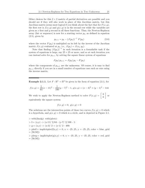
2.1 Newton-Raphson for Two Equations in Two Unknowns 21Other choices for this 2×2 matrix of partial derivatives are possible and youshould see if they will also work in place of this Jacobian matrix, but thisJacobian matrix seems most logical if you think about the fact that for F(x,y),the first row is f(x,y) and g(x,y) is in the second row while the variables aregiven as x first and y second in all these functions. Thus, the Newton-Raphsonarray (list or sequence) is now for a starting vector p 0 , as defined in equation(2.5), given byp k+1 = p k −(J(p k )) −1 F(p k ) (2.8)where the vector F(p k ) is multiplied on its left by the inverse of the Jacobianmatrix J(x,y) evaluated at p k , i.e., J(p k ) = J(x k ,y k ).Note that finding (J(p k )) −1 in each iteration is a formidable task if thesystem of equations is large, say 25×25 or more, and so at each iteration youcan instead solve for p k+1 by solving the square linear system of equationsJ(p k )p k+1 = J(p k )p k −F(p k )where the components of p k+1 are the unknowns. Of course, it is easy to findp k+1 directly if you are in a small number of equations case such as ours usingthe inverse matrix.Example 2.1.1. Let F : R 2 → R 2 be given in the form of equation (2.1), forf(x,y) = 1 64 (x−11)2 − 1100 (y −7)2 −1, g(x,y) = (x−3) 2 +(y −1) 2 −144[ ] 0We wish to apply the Newton-Raphson method to solve F(x,y) = or0equivalently the square systemf(x,y) = 0, g(x,y) = 0The solutions are the intersection points of these two curves f(x,y) = 0 whichis a hyperbola, and g(x,y) = 0 which is a circle, and is depicted in Figure 2.1.> with(linalg): with(plots):> f:= (x,y) -> (x-11)ˆ2/64 - (y-7)ˆ2/100 - 1:> g:= (x,y) -> (x-3)ˆ2 + (y-1)ˆ2 - 400:> plotf:= implicitplot(f(x,y) = 0, x = -25..25, y = -25..25, color = blue, grid= [50,50]):> plotg:= implicitplot(g(x,y) = 0, x = -25..25, y = -25..25, color = red, grid= [50,50]):