LOOP TRANSFER RECOVERY FOR GENERAL ... - CiteSeerX

CONTROL-THEORY AND ADVANCED TECHNOLOGYVol. 8, No.1, pp.59-100, March, 1992C91009R@MITA PRESSLOOP TRANSFER RECOVERY FORGENERAL NONMINIMUM PHASE NON.STRICTLY PROPER SYSTEMS,PART l-ANALYSIS*B. M. CHEN,1 A. SABERIl AND P. SANNUTI2Abstract. A complete analysis of loop transfer recovery (LTR) using full orderobserver based controllers for general nonstrictly proper systems is considered.The given system need not be left invertible and of minimum phase. Our analysis ofLTR focuses on four fundamental issues. The first issue is concerned with what canand what cannot be achieved for a given system and for an arbitrarily specifiedtarget loop transfer function. On the other hand, the second issue is concerned withthe development of necessary and/or sufficient conditions a target loop has tosatisfy so that it can either exactly or asymptotically be recovered for a givensystem while the third issue is concerned with the development of necessary and/orsufficient conditions on a given system such that it has at least one, either exactlyor asymptotically, recoverable target loop. The fourth issue deals with a generalizationof all the above three issues when recovery is required over a subspace of thecontrol space. It concerns with generalizing the traditional LTR concept to sensitivityrecovery over a subspace and deals with method(s) to test whether projectionsof target and achievable sensitivity and complimentary sensitivity functions onto agiven subs pace match each other or not. Such an analysis pinpoints the limitationsof the given system for. the recovery of arbitrarily specified target loops via fullorder observer based controllers. These limitations are the consequences of thestructural properties (i.e., finite and infinite zero structure, and invertibility) of thegiven system. Also, the conditions developed here on a target loop transferfunction for its recoverability, turn out to be constraints on its finite and infinitezero structure as related to the corresponding structure of the given system.Furthermore, the analysis given here discovers a multitude of ways in whichfreedom exists to shape the loops in a desired way as close as possible to the targetshapes. Also, possible pole zero cancellations between the eigenvalues of thecontroller and the input and/or output decoupling zeros of the given system arecharacterized.Key Words~Loop transfer recovery, robust control.1. IntroductionIn classical as well as modern feedback control system design, manyperformance and robust stability objectives can be cast in terms of maximummagnitude or maximum singular values of some particular closed-looptransferfunctions, e. g., sensitivity and complimentary sensitivity functions at certain* Received by the editors January 21, 1991 and in revised form November 9, 1991.*lThe work of B.M. Chen and A. Saberi is supported in part by Boeing Commercial Airplane Group.1 School of Electrical Engineering and Computer Science, Washington State University, Pullman,WA 99164-2752, U.S.A.2 Department of Electrical and Computer Engineering, P. O. Box 909, Rutgers University,Piscataway, NJ 08855-0909, U.S.A.59

60 B. M. CHEN, A. SABERIANDP. SANNUTIpoints in a closed-loop. A principle idea of "loop shaping" is that such magnitudeor singular value requirements on some closed-loop transfer functions can bedirectly determined by corresponding singular values of certain related openlooptransfer functions. A prominent design methodology for multivariablesystems which is based on such loop shaping concepts is LQG/LTR. Historically,LQG/LTR design philosophy involves two steps. The first step is to design astate feedback law that yields an open-loop transfer function which accommodatessatisfactorily the given design specifications on the required sensitivityfunctions. Such an open-loop transfer function is called a target open-looptransfer function. The second step, called loop transfer recovery (LTR),involves the design of an output feedback control law such that the resultingopen-loop transfer function would be either exactly or approximately the sameas the target open-loop transfer function. In other words, the idea of LTR is tocome up with a measurement feedback compensator, typically observer based,to recover a specific open-loop transfer function prescribed in terms of a statefeedback gain.The above mentioned loop transfer recovery (LTR) procedure as a multivariablerobust control design tool has gained significance since the seminal work ofDoyle and Stein (1979). It has been studied by a number of authors includingAthans (1986), Chen et al. (1990; 1991 a; b), Doyle and Stein (1981), Goodman(1984), Matson and Maybeck (1991), Niemann and Jannerup (1990), Niemann etal. (1991), Ridgely and Banda (1986), Saberi et al. (1991 a; b), Sogaard-Andersen (1989), Sogaard-Andersen and Niemann (1989), Saberi and Sannuti(1990 a), Stein and Athans (1987) and Zhang and Freudenberg (1990). Earlierliterature on LTR concentrates on left invertible and minimum phase systemssince this is the only class of systems for which asymptotic LTR is possible foran arbitrarily specified target loop transfer function. A variety of issues arise inanalyzing the LTR mechanism in nonminimum phase systems. Recent works,Chen et al. (1991 b), Niemann and Jannerup (1990), Saberi et al. (1991 a; b) andZhang and Freudenberg (1990), focus on some of these issues. For example, theissues discussed in Saberi et al. (1991 a) and Chen et al. (1991 b) include, (a)Characterizing the available freedom in designing controllers for a given systemand for an arbitrarily specified target loop transfer function, (b) Development ofnecessary and/or sufficient conditions a target loop has to satisfy so that it caneither exactly or asymptotically be recovered for a given system, (c) Developmentof necessary and/or sufficient conditions on a given system such that it hasat least one recoverable (either exactly or asymptotically) target loop and (d)Development of methodes) to test whether recovery is possible in a givensubspace of the control space or not, i.e., to test whether projections of targetand achievable sensitivity and complimentary sensitivity functions onto a givensubspace match each other or not, and in so doing generalizing the traditionalnotion of LTR. The theory developed in Saberi et al. (1991 a) to analyze theissues (a), (b) and (d) is fairly complete when full order observer basedcontrollers are used and when strictly proper systems which are not necessarilyleft invertible and of minimum phase are considered. On the other hand, whengeneral controllers which are not necessarily observer based are used, Chen etal. (1991 b) develops the necessary and sufficient conditions on a strictly propersystem so that it has at least one, either exactly or asymptotically, recoverabletarget loop. As far as design is concerned, there exists essentially threemethods of designing observer based controllers for LTR. These methods are,

Loop transfer recovery, Part I-Analysis 61(1) Kalman filter formalism (Doyle and Stein, 1979), (2) direct eigenstructureplacement method (Sogaard-Andersen, 1989) and (3) asymptotic eigenstructureand time-scale structure assignment (ATEA) method (Saberi and Sannuti,1990 a; Saberi et aI., 1991 b).All the above discussion pertains only to strictly proper systems. Regardingnon strictly proper systems, the only work so far has been by Chen et al. (1990)who consider only left invertible and minimum phase systems. When a givensystem is nonstrictly proper and non necessarily left invertible and of minimumphase, although some aspects of Saberi et al. (1991 a) and Chen et al. (1991 b)carryover in a straight forward manner, other aspects of Saberi et al. (1991 a)present complexities which need to be examined carefully. As such, theintention of this paper is to analyze systematically the LTR mechanism using fullorder observer based controllers in its generality for nonstrictlY proper systemswhich are not necessarily left invertible and of minimum phase. The basicmethodology and the tools used here are akin to those in Saberi et al. (1991 a)and Chen et al. (1991 b). Also, this paper concerns itself only with the analysisof LTR mechanism. A sequel to this paper focuses on the design issues.In order not to lengthen the paper, we concentrate throughout this paperonly on full order observer based controllers. Structure of a controller canimpact the recovery process in more than one way. For example, as seen inChen et al. (1991 a), the size of a gain required for the same degree ofasymptotic recovery can be vastly different in different controllers; also, the setof exactly recoverable target loop transfer functions can be enlarged by using areduced order observer based controller instead of a full order observer basedcontroller. Most of the results developed here for the case of full order observerbased controllers can easily be extended to other controller structures; however,some results need a careful reexamination.Throughout the paper, A' denotes the transpose of A, A H denotes thecomplex conjugate transpose of A, I denotes an identity matrix while I k denotesthe identity matrix of dimension k x k. )"(A) and Re[A(A)] respectively denotethe set of eigenvalues and real parts of eigenvalues of A. Similarly, Gmax[A]andGmin[A] respectively denote the maximum and minimum singular values of A.Ker[V] and Im[V] denote respectively the kernel and the image of V. The openleft and closed right half s-planes are respectively denoted by C- and C +. Also,Rp denotes the sub-ring of all proper rational functions of s while the set ofmatrices of dimension 1x q whose elements belong to Rp is denoted byM1xq(Rp).2. Problem FormulationIn this section, we formulate the LTR problem in precise mathematicalterms. Let us consider a nonstrictly proper system 1:,x = Ax + Bu, y = Cx + Du, (2.1)where the state vector xE~n, output vector yE~P and input vector uE~m.Without loss of generality, assume that [B', D']' and [C, D] are of maximalrank. Let us also assume that 1: is stabilizable and detectable. In this paper, forsimplicity, we concentrate on a case when plant uncertainties are modelled atthe input point of a nominal plant model and hence the required loop transfer

62 B. M. CHEN. A. SABERIANDP. SANNUTIfunction is specified at the plant input point. However, our results can begeneralized easily for the case when the required loop transfer function isspecified at any arbitrary point. In fact, for the case when the required looptransfer function is specified at the plant output point (Kwakernaak, 1969), ourresults can easily be dualized. Let F be a full state feedback gain matrix suchthat (a) the closed-loop system is asymptotically stable, i. e., eigenvalues ofA - BF lie in the left half s-plane, and (b) the open-loop transfer function whenthe loop is broken at the input point of the given system meets some givenfrequency dependent specifications. The state feedback control isu = - Fx, (2.2)and the loop transfer function evaluated when the loop is broken at the inputpoint of the given system, the so called target loop transfer function, isLt(s) = FC/JB, (2.3)where C/J= (sf - A)-I. Arriving at an appropriate value for F is concerned withthe issue of loop shaping which is an engineering art and often includes the use oflinear quadratic regulator (LQR) design in which the cost matrices are used asfree design parameters to generate the target loop transfer function Lt(s) andthus the desired sensitivity and complementary sensitivity functions. The nextstep of design is to recover the target loop using only a measurement feedbackcontroller. This is the problem of loop transfer recovery (LTR) and is the focusof this paper. To explain it clearly, consider the configuration of Fig. 2.1 whereC(s) and P(s),P(s) = CC/JB+ D,are respectively the transfer functions of a controller and of the given system.Given P(s) and a target loop transfer functionLt(s), one seeks then to design aC(s) such that E(s),E(s) == Lt(s) - C(s)P(s),is either exactly or approximately equal to zero in the frequency region ofinterest while guaranteeing the stability of the resulting closed-loop system.Hereafter, we willcallE(s) as recoveryerror. Achievingexact LTR(ELTR), i.e.,rendering the recovery error exactly zero, is in general not possible even for leftinvertible and minimumphase systems. One seeks then approximate LTR. Thenotion of "approximate" LTR has to be defined a little carefully. Here we seek0 u y+-uFig. 2.1. Plant-Controllerclosed-loopconfiguration.

Loop transfer recovery, Part I-Analysis 63achieving LTR to any arbitrarily desired accuracy. In an attempt to make thisfeasible, one normally parameterizes C(s) as a function of a scalar parameter aand thus obtains a family of controllers C(s, a). We say asymptotic LTR (ALTR)is achieved if C(s, a)P(s)~Lt(s) pointwise in s as a~oo, Le., E(s, a)~Opointwise in s as a~ 00. Achievability of ALTR enables the designer to choose amember of the family of controllers that corresponds to a particular value of awhich achieves a desired level of recovery. Traditionally, in observer basedcontrollers, such a parameterization is done by adding a fictitious process noiseof intensity proportional to a which is injected into the system through the inputinto the plant. Then, the observer gain is calculated by solving the resultingfilter algebraic Riccati equations (AREs). In an asymptotic and time-scalestructure assignment (ATEA) procedure of Saberi and Sannuti (1990 a) andSaberi et al. (1991 b), appropriate parameterization of a controller assigns achosen time-scale structure to the resulting closed-loop system. The relativefastness of fast time-scales is then adjusted as desired by tuning the parametera. We now consider the following definitions in order to impart precise meaningsto ELTR and ALTR.Definition 2.1. The set of admissible target loops T(1:') for the givensystem 1:'is defined byT(1:') = {Lt(s) E Mmxm(Rp) ILt(s) = FtPB and A(A-BF) E C-}.Definition 2.2. Lt(s)ET(1:') is said to be exactly recoverable (ELTR) ifthere exists a C(s)EMmXP(Rp) such that (i) the closed-loopsystem comprisingof C(s) and P(s) as in the configurationof Fig. 2.1 is asymptotically stable, and(ii) C(s)P(s)=Lt(s).Definition 2.3. Lt(s) E T(1:') is said to be asymptotically recoverable(ALTR) if there exists a parameterized family of controllers C (s, a)EMmXP(Rp), where a is a scalar parameter taking positive values, such that (i)the closed-loop system comprisingof C(s, a) and P(s) as in the configurationofFig. 2.1 is asymptotically stable for all a> a*, where 0:$a*< 00,and (ii) C(s,a)P(s)~Lt(s) pointwise in s as a~oo. Moreover, the limits, as a~oo, of thefinite eigenvalues of the closed-loop system should remain in C-t.Definition 2.4. Lt(s) belonging to T(1:') is said to be recoverable if Lt(s) iseither exactly or asymptotically recoverable.Definition 2.5.1. The set of exactly recoverable target loops for the given system 1:' isdenoted by TER(1:').2. The set of recoverable target loops for the given system 1:'is denoted byTR(1:').3. The set of target loops which are asymptotically recoverable but not exactlyrecoverable for the given system 1:'is denoted by TAR(1:').Obviously, TR(1:')= TE\1:') U TAR(1:').It is well known that for left invertible and minimum phase systems, anyt Here we have strengthened the notion of the closed-loop stability in order to exclude those caseshaving the limits, as u-> 00, of some finite eigenvalues of the closed-loop system being on the j waxis. This avoids havingan almost unstable behavior of the closed-loopsystem for large u.

64 B. M. CHEN, A. SABERIANDP. SANNUTIarbitrary admissible target loop is asymptotically recoverable and hence TR(.l')is equal to T(.l'). On the other hand, if the given system .l' is not left invertibleand/or of nonminimum phase, not all target loops are recoverable, i. e., TR(.l') isnot equal to T(.l'). In fact, TR(.l') might be an empty set. As mentioned in theintroduction, the purpose of this paper is to analyze the LTR mechanismsystematically for the general system.l' given by (2.1) when the controller C(s)or C(s, a) uses a full order observer based structure. All the results given inthis two part paper pertain only to the case when full order observer basedcontrollers are used. In general, all the issues involved in attempting to recovera target loop transfer function depend on the architecture of the controller. Forexample, as is evident from Theorems 1 and 2 of Chen et al. (1991 a), the set ofexactly recoverable target loops when reduced order observer based controllersareused is different from that when full order observer based controllersare used. As such the results of this paper require several modificationswhenever the architecture of the controller is other than the full order observerbased controller. Analysis of LTR mechanism using reduced order observerbased architecture or any other compensator architecture such as the onedeveloped in Chen et al. (1991 a), is a topic of future research.The analysis of LTR mechanism carried out here focuses on four fundamentalissues. The first issue is concerned with what can and what cannot be achievedfor a given system and for an arbitrarily specified target loop transfer function.On the other hand, the second issue is concerned with the development ofnecessary and/or sufficient conditions a target loop has to satisfy so that it canbe either exactly or asymptotically be recovered for a given system while thethird issue is concerned with the developm.ent of necessary and/or sufficientconditions on a given system such that it has at least one recoverable (eitherexactly or asymptotically) target loop. The fourth issue deals with a generalizationof all the above three issues when recovery is required over a subspace ofthe control space. It concerns with generalizing the traditional LTR concept tosensitivity recovery over a subspace and deals with method(s) to test whetherprojections of target and achievable sensitivity and complimentary sensitivityfunctions onto a given subspace match each other or not. All this analysis showssome fundamental limitations of the given system as a consequence of itsstructural properties, namely finite and infinite zero structure and invertibility.It also discovers a multitude of ways in which freedom exists to shape therecovery error in a desired way. Thus, it helps to set meaningful design goals atthe onset of design.The paper is organized as follows. As is evident from Saberi and Sannuti(1990 a) and Saberi et al. (1991 a), the finite and infinite zero structure of agiven system plays a dominant role in LTR. Recognizing this, in Sec. 3, we recalla special coordinate basis (s.c.b) of Sannuti and Saberi (1987) and Saberi andSannuti (1990 b) which displays clearly the required zero structure. Section 4deals with analysis for an arbitrarily given target loop. This analysis includes notonly the recovery of a target loop transfer function but also target sensitivity andcomplimentary sensitivity functions. We show that either ELTR or ALTR ingeneral is not possible. Whenever LTR is not possible, we give explicitexpressions for the asymptotic limits of loop transfer function and sensitivityand complimentary sensitivity functions. Moreover, we give explicit bounds onthe attainable sensitivity and complimentary sensitivity functions in terms of thesingular values of what is called a recovery error matrix to be defined later on.

Loop transfer recovery, Part I-Analysis 65These bounds can be used to analyze the inevitable trade-off between the goodrecovery as indicated by the maximum singular value of the recovery errormatrix, and robustness and performance as reflected in the sensitivity andcomplimentary sensitivity functions. We next move on to the characterization ofa subspace in which the target sensitivity and complimentary sensitivityfunctions can be recovered. All the analysis given here treats the target looptransfer function L/s) as an arbitrarily given matrix, i.e., no particularproperties of Lt(s) are exploited in the analysis. However, in Sec. 5, we takeinto account the specific characteristics Lt(s) might have. Here the necessaryand sufficient conditions under which Lt(s) can either exactly or approximatelybe recovered are given. Interestingly enough, these constraints turn out to beconstraints on the finite and infinite zero structure of it. Such an interpretationof the constraints reveals that either ELTR or ALTR is possible under a varietyof conditions. Also, in this section we establish the necessary and/or sufficientconditions on the given system so that it has at least one recoverable targetloop. In fact, following Chen et al. (1991 b), given a general non strictly propersystem which is not necessarily left invertible and of minimum phase, weconstruct here an auxiliary system from it and show that the set of recoverabletarget loops for the given system is nonempty, if and only if the auxiliary systemis stabilizable by a static output feedback controller. This then leads to a simpleand surprising necessary condition on the given system, namely, strong stabilizabilityt of the given nonminimum Phase system is a necessary condition for it tohave at least one recoverable target loop. However, the fact that the given systemis strongly stabilizable itself does not guarantee that there exists at least onerecoverable target loop. The analysis given in Secs. 4 and 5 stresses recoverabilityin the entire control space f!Jlm.On the other hand, Sec. 6 generalizes allthe results developed in Secs. 4 and 5 in order to cover recoverability of thetarget sensitivity and complimentary sensitivity functions in a specified subspaceand thus adds a considerable amount of flexibility to the process of design.It also shows that for left invertible systems irrespective of the number ofnonminimum phase zeros and irrespective of the nature of the target looptransfer function, there exists at least one m -1 dimensional subspace of f!Jlminwhich the target sensitivity and complimentary sensitivity functions can alwaysbe recovered by an appropriate design of the controller. Also, in Secs. 4 and 5,under all the analysis conditions given above, the resulting controller eigenvaluesand possible pole zero cancellations are clearly discussed. Finally in Sec. 7,we draw conclusions of our work.3. PreliminariesAs is evident from Saberi et al. (1991 a; b), finite and infinitezero structuresof both the given system and the target loop transfer function playa dominantrole in the recovery analysis as wellas design. Keeping this in mind, we recall inthis section a special coordinate basis (s.c.b) of a linear time invariant system(Sannuti and Saberi, 1987; Saberi and Sannuti, 1990 b). Such an s.c.b has adistinct feature of explicitly displayingthe finite and infinite zero structure of agiven system. Consider the system ~ characterized by (A, B, C, D). It issimple to verify that there exist non-singular transformations U and V such thatt A system is said to be strongly stabilizable if there exists a stable and proper compensatorstabilizes the system (Vidyasagar, 1985).which

66 B. M. CHEN, A. SABERIANDP. SANNUTIUDV = [ 10° ~ J.(3.1)where mois the rank of matrix D. Hence hereafter, without loss of generality, itis assumed that the matrix D has the form given on the right hand side of (3.1).One can now rewrite the system of (2.1) as,X =Ax + [Bo Bd[uo un', (3.2a)[ ~; ] = [ g; ]x + [10° ~][:; J.(3.2b)where the matrices Bo, Bb Co and C1 have appropriate dimensions. We havethe followingtheorem.Theorem 3.1. (s.c.b). Consider the system 2: characterized by (A, B, C,D). There exist nonsingular transformations r1, rz and r3, an integermfS m - mo, and integer indexes qi' i = 1,.. .,mf, such thatx = r1x, Y = rzy, u = r3u,x = [x~, Xb, x~, xj]',- " ,[]'xf = Xl, Xz, ..., Xmf 'Xa = [(x~)', (x;)']',y = [y~,Y;, y;]',Yf= [Y1'Y2' ...,ym)',u= [UO, U;, U~]', Uf= [Ub Uz, ..., Um)'andX~ = A~ax;; + BoaYo + L~fYf + L~bYb' (3.3). +A + + B + + L + + L +Xa = aaXa + OaYo afYf abYb,(3.4)ib = AbbXb + BObYo + LbfYf' Yb = CbXb, (3.5)Xc = Accxc + BOcYO+ LcbYb + LcfYf + BAE~ax;;+E:ax;] + Bcuco (3.6)Yo= COax;; + C6aX; + CObXb+ COcXc+ COfXf + Uo (3.7)and for each i= 1,''',mf,Xi = AqXi + LioYo + LifY. f~+ Bq [ui+Eiaxa+EibXb+Eicxc+~ Eijxj],iJ=ly. = C q Xi,t i Yf = Cfxf'(3.8)(3.9)Here, the states x;;, Xd, Xb, Xcand xfare respectively of dimension n;;, n;, nb,

Loop transfer recovery, Part I-Analysis 67ne and nf= 'L;':;lqi while Xi is of dimension qi for each i= 1,''', mr The controlvectors Uo, uf and Ueare respectively of dimension mo, mf and me= m - mo- mfwhile the output vectors Yo' Yf and Yb are respectively of dimension po=mo,Pf=mfandPb =P-Po -Pr The matrices Aq;, Bqi and Cqihave the following form:A Iqi-l0B qi - [ 0 0 ] ' qi - [ l' ]Cqi = [1, 0, "', 0]. (3.10)(Obviously for the case when qi=l, we have Aq=O, Bq=l and Cq=1.)Furthermore, we have )..(A;;a)EC-, ).(A;a)EC+, the pair (A~c>Be) is controllableand the pair (Abb, Cb) is observable. Also, assuming that Xi are arrangedsuch that Qi:5Qi+l' the matrix Lifhas the particular form,Lif = [Lit. Liz, ..., Lii-t. 0, 0, ..., 0].Also, the last row of each Lif is identically zero.Proof. This follows from Theorem 2.1 of Sannuti and Saberi (1987) and Saberiand Sannuti (1990 b).We can rewrite the s. c.b given by Theorem 3.1 in a more compact form,A;;a 0 L;;bCb 0 L;;fCf0 A;a L;b Cb 0 L;fCfA ri1(A-BoCo)r1 = I0 0 Abb 0 LbfCf I'BeE;;a BeE-:a LebCb Ace LefCfBfE;; BfE; BfEb BfEe AfBoa 0Bta 0jj ~ ri1[Bo B1]r3 = I BOb 0Boe 0BOf Bf000Be0- -1C ~ rZ r1 = 0 0 0 0 Cf[CoCOa cta COb COe COfC1 ] [ 0 0 Cb 0 0]andImojj ~ r21Dr3 = ~[000 HIn what follows, we state some important properties of the s.c.b which arepertinent to our present work.Property 3.1. The given system 2: is right invertible, if and only if Xbandhence Yb are nonexistent (nb=O, Pb=O), left invertible, if and only if Xcandhence Ueare nonexistent (ne=O, me=O), invertible, if and onlyif both Xband Xcare nonexistent. Moreover, 2: is degenerate, if and only if it is neither left norright invertible.

68 B. M. CHEN, A. SABERIANDP. SANNUTIProperty 3.2. We note that (Abb, Cb) and (Aq, Cq) form observable pairs.Unobservability could arise only in the variables x~ and' XC'In fact, the system ~is observable (detectable), if and only if (Aobs, Cobs) is an observable (detectable)pair, whereAaa 0A- 0COa Coeaa ,Aobs = [ BeEea Ace' ] Aaa = [ 0 A':;a ] Cobs = [ E a E e ] 'COa = [COa, cta], Ea = [E;;, E':;], Eea = [E-;;a,E:-a].Similarly, (Ace> Be) and (Aq, Bq) form controllable pairs. Uncontrollabilitycould arise only in the variables Xaand Xb' In fact, ~is controllable (stabilizable),if and only if (Aeon, Beon) is a controllable (stabilizable) pair, whereA =[Aaa LabCbBOa Latcon 0 Abb ] ' Beon = [ BOb Lbt ] 'BOaL;;bL;;t+,BOa - [ BOa ] Lab = [ L':;b ] ' Lat = [ L':;t ] .Property 3.3. Invariant zeros of ~ are the eigenvalues of Aaa. Moreover,the stable and the unstable invariant zeros of ~ are the eigenvalues of A;;aandA':;a,respectively.There are interconnections between the s.c.b and various invariant andalmost invariant geometric subspaces. To show these interconnections, wedefineVg(A, B, C, D)-the maximalsubspace of 'lllnwhich is (A - BF)-invariantand contained in Ker( C - DF) such that the eigenvalues of (A - BF) Ivg arecontained in Cg~ C for some F.Sg(A, B, C, D)-the minimal(A - KC)-invariant subspace of'lllncontainingin Im(B - KD) such that the eigenvalues of the map which is induced by(A-KC) on the factor space 'llln/sg are contained in Cg~C for some K.For the cases that Cg=C, Cg=C- and Cg=C+, we replace the indexg in vgand sg by "*", "-" and "+", respectively. Various components of the statevector of s. c.b have the followinggeometrical interpretations.Property 3.4.1. x;;EE>x':; EE>xe spans V*(A, B, C, D).2. x;;EE>xespans V-(A, B, C, D).3. x,:;EE>xespans V+(A, B, C, D).4. xeEE>Xt spans S*(A, B, C, D).5. X;;EE>xe EE>Xt spans S+(A, B, C, D).6. x':;EE>xeEE>Xt spans S-(A, B, C, D).4. General AnalysisAs mentioned in the introduction, throughout this paper, we will consideronly full order observer based controllers as depicted in Fig. 4.1. The dynamicequations of the controller are

Loop transfer recovery, Part I-Analysis 69r u y+ .--ur ---Controller - - +-lI D IIIIIIIII+ IIII - IIII C IIIl- - - JFig. 4.1. Plant with full order observer based controller.i = Ax + Bu + K(y-Cx-Du)andu = u = - Fx,where K is the observer gain and F is the state feedback gain whichprescribesthe target loop transfer function Lt(s)=F(/JB. The transfer function of thecontroller isC(s)= F[sIn-A+BF+KC-KDF]-lK,while the loop transfer function realized by the controller isLo(s) = C(s)P(s).The recoveryerror E(s) isE(s) = Lt(s) - Lo(s). (4.1)A brief outline of this section is as follows. The expression for the recoveryerror E(s) as given by (4.1) is not well suited for loop transfer recoveryanalysis. Realizing this, we first relate E(s) to a matrix, hereafter called asrecovery matrix, M(s)=F(sIn-A+KC)-l(B-KD), and then show thatE(jw)=O, if and only if M(jw) =0. This implies that a general loop transferrecovery (LTR) analysis is synonymous with a general study of the recoverymatrix M(s) whichobviouslyis dependent explicitlyboth onK andF. A physicalinterpretation of M(s) can be given. Considering the observer based controlleras a device with its inputs as the plant input and the plant output, -M(s) is thetransfer function from the plant input point to the controller output point. Thus,whenever LTR is achieved, the controller output does not entail any feedbackfrom the plant input point. The needed study of M(s) to ascertain how and whenit can be rendered zero, can be undertaken in two ways, with or without theprior knowledge of F that prescribes the target loop transfer function Lt(s).Note that the study of M(s) without the prior knowledge of F imitates the

70 B. M. CHEN, A. SABERIANDP. SANNUTItraditional LQG design philosophy in which the two tasks of obtainingF and Kare separated. Keeping this in mind, our goal in this section is to study M(s)without taking into account any specific characteristics of F. The next section,devoted to LTR analysis while taking into account appropriate characteristics ofF, complimentsthe analysis of this section. Here, in order to study the recoverymatrix M(s) without havingthe knowledge ofF, we decompose M(s) as FM(s)where M(s)= (sIn -A + KC)-l(B -KD). A detailed study of M(s) inthis sectionleads to two fundamental lemmas, one dealing with finite and another dealingwith asymptotically infinite eigenstructure assignment to the observer dynamicmatrix A-KC by an appropriate design of K. These two lemmas reveal thelimitations of the given system as a consequence of its structural properties inrecovering an arbitrary target loop transfer function via a full order observerbased controller. Furthermore, they enable us to decompose M(s) into threeessential parts, MO(s), MCO(s)and Me(s). The first part MO(s) can be renderedeither exactly or asymptotically zero by an appropriate finite eigenstructureassignment to A - KC, whilethe second part MCO(s)can be rendered asymptoticallyzero by an appropriate infinite eigenstructure assignment to A - KC. Thethird part Me(s) in general cannot be rendered zero, either exactly or asymptotically,by any means, although our analysis of Me(s) reveals a multitude of waysby whichit can be shaped. Allin all, the decompositionof M(s) into various partsand the subsequent analysis of each part forms the core of entire analysis giventhroughout this paper. In particular, it leads to several important results given inthis section. For example, Theorem 4.1 characterizes the asymptotic behaviorof loop transfer function as well as sensitivity and complimentary sensitivityfunctions achievable by full order observer based controllers. On the otherhand, Theorem 4.2 shows the subspace seE£nm in whichMe(s) can be renderedzero asymptotically, i.e., the projections of the target and achievable sensitivityand complimentary sensitivity functions onto se can match each other asymptotically.Furthermore, our analysis in this section reveals the mechanism ofpole zero cancellation between the controller eigenvalues and the input oroutput decoupling zeros of 2: for the case when F is unknown.We will now proceed with the analysis. We have the following lemma, ageneralization of the result due to Goodman(1984).Lemma 4.1. Consider any arbitrary F such that A - BF is asymptoticallystable. Then E(s), the error between the target loop transfer functionLis) andthat realized by the controller of Fig. 4.1, is given bywhere the recovery matrix,Furthermore for all wE Q,E(s) = M(s)[Im+M(s)]-l(lm+F

ProofSee AppendixA.Loop transfer recovery, Part I-Analysis 71In order to give a physical meaning to M (s), one can redraw Fig. 4.1 aseither Fig. 4.2 or Fig. 4.3 where the controller is viewed as a device havingtwoinputs, (1) the plant input u and (2) the plant output y. When the controller isviewed havingtwo inputs u andy, -M(s) is the transfer functionfrom the plantinput point to the controller output point whileM(s) is the transfer functionfromthe plant input point to the estimated state x. In particular, for full orderobserver based controller of Fig. 4.1, we havex(s) = M(s)u(s)+ N(s)y(s)andu(s) = -Fx(s) = -M(s)u(s) - N(s)y(s), (4.5)whereM(s) = (sIn-A+KC)-l(B-KD), M(s) = FM(s) (4.6)andN(s) = (sIn-A+KC)-lK,N(s) = FN(s).yuFig. 4.2. Plant and observer configuration.yuII I I IIL_-------Controller.JIFig. 4.3. Plant and controller configuration.

72 B. M. CHEN, A. SABERIANDP. SANNUTIThe above equations show that -M(s) is the transfer function from the plantinput point to the controller output point when controller is treated having twoinputs, u and y. Lemma 4.1 implies then that whenever LTRis a,chievedby thecontroller, the controller output does not entail any feedback from the plantinput point.Equations (4.3) and (4.4) present a clear perspective to study the basicmechanism of LTR. In fact, they facilitatethe study of E (s) in terms of the studyof M(s). Thus, Lemma 4.1 and the expression for M(s) as given by (4.3) form abasis for our study. Since in this section, F is considered as arbitrary orunknown, the only freedom we have to achieve the needed recovery is in theselection of observer gain K. First of all, in view of the well known separationprinciple, in order to guarantee the closed-loop stability, K must be such that theobserver dynamic matrix, A - K C is an asymptotically stable matrix. Theremaining freedom in choosingK can then be used for the purpose of achievingLTR. Now in view of (4.3) and (4.4), exact loop transfer recovery (ELTR) ispossible for an arbitrary F, if and only ifM(jw) = (jwIn-A+KC)-1(B-KD) == O.However, due to the nonsingularity of (j wIn- A +K C)-I, the fact that£1(j w) == 0 implies that B - KD ==O. The class of systems in which B - KD can berendered exactly zero is restrictive, and hence one normallyattempts to achieveasymptotic loop transfer recovery (ALTR), i.e., to render £1(j w) approximatelyzero in some sense. In order to analyze whether ALTRis possible, as mentionedin the introduction, we parameterize the gain K with a tuning parameter a andthus consider a familyof controllers,C(s, a) = F[sIn-A+BF+K(a)C-K(a)DF]-1K(a). (4.7)Now M(s) and M(s) are also functions of a and are denoted respectively byM(s, a) and M(s, a). To proceed with our analysis, for clarity of presentationwe will temporarily assume that A - KC is nondefective. This allows us toexpand M(s, a) and hence M(s, a) in a dyadic form,- n-M(s, a) = ~~i=1 s-Ai '(4.8)where the residue R i is given by- HRi = WiVdB-K(a)D]. (4.9)Here Wi and Vi are respectively the right and left eigenvectors associated withan eigenvalue Ai of A - K C and they are scaled so that WVH= VHW= In whereW= [Wi> W2, ..., Wn] and V = [Vi>V2, ..., Vn]. (4.10)In general, all Ai, Vi and Wi are functions of a. However, for economy ofnotation we willnot show the dependence on a explicitlyunless it is needed forclarity.

Loop transfer recovery, Part I-Analysis 73Remark 4.1: The assumption that K(a) is selected so that A-K(a)C isnondefective is not essential. However, it simplifies our presentation. Aremoval of this condition necessitates the use of generalized right and lefteigenvectors of A - K (a) C instead of the right and left eigenvectors Wiand Viand consequently the expansion of M(s, a) requires a doublesummationin placeof the single summation used in (4.8).Weare lookingfor conditionsunder whichfor each i= 1, . .. ,n, the ith term ofM(s, a) in (4.8) can be made zero. There are only two possibilities to do so.1. The first possibility is by assigning Ai to any finite value in C- whilesimultaneously rendering- the corresponding residue Ri zero either exactlyH -or asymptotically, i.e., Ri= Wi(a)Vi (a)[B -K(a)D]=O or Ri~O as a~ 00.Thus, this possibility deals with finite eigenstructure assignment ofA-K(a)C.2. The second possibility is to make Ri/(s-Ai)~O pointwise in s as a~oo.This can be done by placing the eigenvalue Ai(a) asymptotically at infinitywhile makingsure that the corresponding residue Ri is uniformly bounded asa~ 00. It is important to recognize that placing Aiasymptotically at infinityalone is not beneficial unless the corresponding residue Ri is bounded. Thisamounts to assigning W/a) and V/a) such that Ri= Wi(a)Vr(a)[B- K (a)D] remains bounded while Ai~ 00 as a~ 00. Thus, this possibilitydeals with infinite eigenstructure assignment of A-K(a)G.The above two possibilities of making a particular term of M(s, a) zero leadsto two fundamental questions that need to be answered: (1) How many lefteigenvectors of A-K(a)C can be assigned to the null space of [B-K(a)D]'?and (2) How many eigenvalues of A - K (a) C can be placed at asymptoticallyinfinite locations in C- so that the corresponding residues are finite? Thefollowing two lemmas respectively answer these two questions. In theselemmas and elsewhere, the geometric spaces S-(A, B, C, D), V*(A, B, C, D)and V+ (A, B, C, D) are as defined in Sec. 3.Lemma 4.2. Let Ai and Vi be an eigenvalue and the corresponding lefteigenvector of A - K (a)C for any gainK (a) such that it is asymptoticallystable.Then, the maximum possible number of AiE C- which satisfy the conditionVr [B - K (a)D] = 0 is n; + nb. A total of n; of these Aicoincidewith the invariantzeros of 2: which are in C- (the so called stable invariant zeros) and theremaining nb eigenvalues can be assigned arbitrarily to any locations in C-. Allthe eigenvectors Vi that correspond to these n; + nb eigenvalues span thesubspace fnn/S-(A, B, C, D). Moreover, the n; eigenvectors Vi whichcorrespond to the eigenvalues which coincide with the system invariant zeros inC- coincide with the corresponding left state zero directions and span thesubspace V*(A, B, C, D)/V+(A, B, C, D).Proof. See Appendix B.Remark 4.2: Instead of rendering the n;+nb residues Ri mentioned inLemma 4.2 exactly zero, if one prefers, they can be rendered asymptoticallyzero as a~ 00. In that case n; eigenvalues coincide asymptotically with the n;;stable invariant zeros while the corresponding eigenvectors in the limit as a~ 00coincide with the corresponding left state zero directions and span the subs paceV*(A, B, C, D)/V+(A, B, C, D).

74 B. M. CHEN, A. SABERIANDP. SANNUTILemma 4.3. Let Ai>Wi and Vibe an eigenvalue and the corresponding rightand left eigenvectors ofA - K(a)C foranygainK(a) suchthat itis asymptoticallystable. The maximum number of eigenvalues of A - K (a) C that can beassigned arbitrarily to asymptotically infinite locations in C- so that thecorresponding R;= Wivf [B - K (a)D] are bounded as IAiI~ 00 is nb + nf'Furthermore, all the corresponding left eigenvectors Vi of such eigenvaluesasymptotically span the subspace qjln/V*(A, B, C, D).Proof.It followsalong the same lines as Lemma 3.3 of Saberi et al. (1991 a).As implied by Lemma 4.2, in addition to n;;eigenvalues which coincidewiththe stable invariant zeros of the given system, there are nb other eigenvalueswhich can be assigned arbitrarily to any locations in C- such that Ri=O. Thisimplies that Ri corresponding to these nb eigenvalues are identically zero andhence are bounded. Thus, these nb eigenvalues are included among the nb+nfeigenvalues indicated in Lemma 4.3. That is, there is a set of nb eigenvalueswhich can be placed arbitrarily at either asymptotically finite locations in C- asindicated by Lemma 4.2 or at asymptotically infinite locations in C- as indicatedby Lemma 4.3. Hereafter, in order to conserve the controller bandwidth, we willassume that these nb eigenvalues are always assigned to asymptotically finitelocations.Remark 4.3: Consider the case when 1: is right invertible and has no infinitezeros. Note that this case includes the special case when 1: is a non-strictlyproper single-input and single-output system (5150). For this case, nb+ nf= 0and hence there is no eigenvalue, Aiof A-K(a)C that can be assigned to aninfinite location such that the corresponding Ri is bounded.Lemmas 4.2 and 4.3 together tell us all the possibilities of rendering variousterms of M(s, a) zero either exactly or asymptotically. There are altogethern;;+ nb+ nf eigenvalues whichcan be assigned either at finite or at asymptoticallyinfinite locations so that the corresponding terms of M(s, a) in its dyadicexpansion (4.8) are either exactly or asymptotically zero. Thus, a questionarises as to under what conditions n;;+ nb+ nf equals the dimension n of thegiven system. It is indeed easy to see that n;;+ nb+ nf= n, if and only if 1: is leftinvertible and of minimumphase. Thus, for left invertible and minimumphasesystems, asymptotic LTRis always achievable irrespective of the properties ofthe given target loop transfer function Lt(s). For strictly proper systems, thisresult is well known (Doyle and Stein, 1979; Matson and Maybeck, 1991).If 1: is not left invertible and/or of nonminimumphase, there are ne=n - n;;-nb-nf=n;; +nc terms of M(s, a) which cannot in ~eneral be rendered zero.To emphasize explicitlythe behavior of each term of M(s, a), we partition it intofour parts,whereM(s, a) = M-(s, a) + Mb(s, a) + MOO(s,a) + Me(s, a), (4.11)andM-(s, a) = ~ R-ii=1 s-ki '-b n.-bM (s, a) = ~~i=1s- Af

Loop transfer recovery, Part l-Analysis 75MOO(s,a) = ~ k;i=l s-),'[' ,n;+n, R~M -e ( ) - ~ ;e.s, a - i=l S-"iIn the above partition, appropriate superscripts -, b, 00 and e are added to Riand),i in order to associate them respectively with M-(s, a), Mb(s, a), MOO(s,a) and Me(s, a). Next, define the followingsets where ne=n; +nc:A-(a) 4 {),i(a) Ii = 1, ''', n~}, Ab(a) 4 {Af(a) Ii = 1, ''', nb},A 00(a) 4 {),'['(a) Ii = 1, "', nl}, Ae(a) 4 {),Ha) Ii = 1, "', ne},V-(a) 4 {Vi(a)li = 1, "', n~}, Vb(a) 4 {Vf(a)Ii = 1, "', nb},VOO(a) 4 {V'['(a) Ii = 1, ''', nl}, pea) 4 {VHa) Ii = 1, "', ne},W-(a) 4 {Wi(a)li = 1, "', n~}, Wb(a) 4 {Wf(a)li = 1, "', nb},WOO(a)4 {W'['(a)Ii = 1, "', nl}, We(a) 4 {WHa)li = 1, "', ne}.Hereafter, we will be using an over bar on a ~ertain variable to denote its limitwhenever it exists as a~ 00. For example, Me(s) and we denote respectivelythe limits of Me(s, a) and We(a) as a~ 00.We now note that various parts of M(s, a) have the following interpretation:1. M-(s, a) contains n~ terms. The n~ eigenvalues of A-K(a)Crepresentedin it form a set A -( a). In accordance with the Lemma 4.2, there exists a gainK(a) such that M-(s, a) can be rendered identically zero by assigning theelements of A -( a) to coincide with the stable invariant zeros of 1: while thecorresponding set of left eigenvectors V-( a) coincides with the correspondingset of left state zero directions. In fact, K(a) can also be designed suchthat A-(a) and V-(a) approach asymptotically the set of system minimumphase invariant zeros an

76 B. M. CHEN, A. SABERIANDP. SANNUTIsets of right and left eigenvectors, We(a) and Ve(a). However, as will bediscussed later on, £1e(s, a) can be shaped to have some desirableproperties. Since (A, C) is assumed to be a detectable pair, except for thestable but unobservable eigenvalues of A, others among the remainingeigenvaluesof A - K(a)C whichare in Ae can be assignedto arbitrarylocations in C-. These arbitrary locations can either be asymptotically finiteor infinite. Moreover, assigning elements of Ae(a) to asymptotically infinitelocations increases unnecessarily controller bandwidth. Because of this, weassume Ae is confined to finite locations in C-.Since both £1-(s, a) and £1b(s, a) can be rendered identically zero, for futureuse we can combine them into one term,and rewrite £1(s, a) as£1O(s, a) = £1-(s, a) + £1b(s, a),£1(s, a) = £1O(s, a) + £1"'(s, a) + £1e(s, a). (4.12)We define likewise, AO(a)=A-(a)UAb(a), WO(a)=W-(a)UWb(a) andVO(a)= V-(a)U Vb(a).As the above discussion indicates, Lemmas 4.2 and 4.3 form the heart of theunderlying mechanism of LTR as they enable us to decompose £1(s, a) andhence M(s, a) into several parts. They show dearly what is and what is notfeasible under what conditions. Although they do not directly provide methodsof obtaining the gain K(a), they do provide structural guide lines as to howcertain eigenvalues and eigenvectors are to be assigned while indicating amultitude of ways in which freedom exists in assigningthe other eigenvalues andeigenvectors of A - K (a) C. These guidelines, in turn, can appropriately bechanneled to come up with a design method to obtain an appropriate gain K(a).As willbe discussed systematically in a paper sequel to this (Chen et al., 1992),there exist essentially three methods of design to obtain appropriate K(a).These are (1) Kalmanfilter formalismwhichminimizesthe H2-normof M(s), (2)Methods of minimizingH",-norm of M(s) and (3) Asymptotic time-scale andeigenstructure assignment (ATE1\.)method of Saberi and Sannuti (:990 a) andSaberi et al. (1991 b) by which £1e(s) can be shaped as desired in a number ofways. Leaving aside now the methods of design, let us at this stage simplydefine a set of gains K*(~, a) as follows:Definition 4.1. K*(~, a) is a set of gains K(a)E.:nnxp such that(1) A-K(a)C is stable for all a>a*, where O:5a*

Loop transfer recovery, Part I-Analysis 77K(a) of K*(1:, a) is dependent on a. Moreover, IIK(a) II~ 00as a~ 00.It is obvious that K*(1:, a) as defined above is a nonempty set. We note alsothat whenever K(q) is chosen as an element of K*(1:, a), the asymptotic limit,namely Me(s)=FMe(s), as a~oo of Me(s, a)=FMe(s, a) is the ultimate errorin the recovery matrix M(s, a). As such, hereafter Me(s) is called as therecovery error matrix. Theorem 4.1 given below characterizes the asymptoticbehavior of the achieved loop transfer function as well as the sensitivity andcomplementary sensitivity functions in terms of Me(s). Let So(s, a) and To(s,a) be the achieved sensitivity and complementary sensitivity functions using theoutput feedback controller C (s, a) as in the configuration of Fig. 4.1 when theloop is broken at the input point of the system,andSo(s, a) = [/m+ C(s, a)P(s)]-lTo(s, a) = 1m - So(s, a) = [/m+ C(s, a)P(s)]-l C(s, a)P(s).Also, let St(s) and Tt(s) be the target sensitivity and complementary sensitivityfunctions corresponding to the target loop transfer function. We have thefollowing theorem.Theorem 4.1. Consider the closed-loop system 1:Ccomprising of the givensystem 1: and the controller as given in Fig. 4.1. Let ;E be stabilizable anddetectable. Then for any F such that A - BF is asymptotically stable, and for anygain K(a)EK*(1:, a), the closed-loop system 1:c is asymptotically stable.Moreover, as a~oo, we have pointwise in s,E(s, a) ~ FMe(s)[lm+FMe(s)]-l(lm+FfPB),So(s, a) ~ St(s) [/m+FMe(s)],(4.13)(4.14)To(s, a) ~ Tt(s) - St(s)FMe(s), (4.15)andIai[So(jw, a)]-ai[St(jw)] I :5 arnax[FMe(jw)],arnax[S/jw)](4.16)lai[To(jw, a)]-ai[Tt(jw)J! :5 arnax[FMe(jw)].arnax[St

78 B. M. CHEN, A. SABERIANDP. SANNUTIProof I is left invertible and of minimumphase implies that n~ =0, nc= O.Since n~+nc=O, jJe(s, a) is nonexistent. Hence the results of Corollary 4.1are obvious.Remark 4.5: For strictly proper systems, the results of corollary are wellknown as given in the seminal work of Doyle and Stein (1979). The results ofCorollary 4.1 for non-strictly proper systems are given in Chen et al. (1990).As implied by Theorem 4.1, the recovery error matrix ife(s) plays adominant role in the recovery process and hense it should be shaped to yield asbest as possible the desired results. Shaping jJe(s) involves selecting the set ofeigenvalues Ae represented in jJe(s) and the associated set of right and lefteigenvectors We and Ve. Such a selection can be done in a number of wayssubject to the constraints imposed in selecting the eigenvectolJ) (Moore, 1976).However, note that though, no shapingw.ay be necessary if jJe(s) turns out tobe small. For certain class of systems Me(s) is, in fact, small in some sense orother. Following a similar result of Saberi et al. (1991 a), one can prove easilythat for a left invertible nonminimum phase system which is not necessarilystrictly proper but which has all its unstable invariant zeros far away from thebandwidth of the target loop transfer function, the norm of the recovery errormatrix jJe(s) is indeed always small.In multivariable systems, one interesting aspect qiTheorem 4.1 is that therecould exist a subspace ofthe control space in whichMe(s) can be rendered zero.To pinpoint this, letei = [B-K(a)D]'Vi, Vi E ve, (4.18)and let Ee be the subspaceof g'lm,Let the dimension of P be me. Now letP = Span{ ei lVi EVe}. (4.19)se = orthogonal complement of Ee in g'lm. (4.20)Let ps be the orthogonal projection matrix onto se. Then the following theorempinpoints the directional behavior of jJ(s, a) and consequently the behavior ofSo(s, a) and To(s, a) as a---'>00.Theorem 4.2. Consider the closed-loop system IC comprising of the givensystem I and the controller as given in Fig. 4.1. Let I be stabilizable anddetectable. Then for any F such that A - BF is asymptotically stable, and for anygain K(a)EK*(I, a), the closed-loop system IC is asymptotically stable.Moreover, considering the subspace seEg'lm as given in (4.20) and denoting theorthogonal projection matrix onto se as ps, we have as a---'>oo,pointwise in s,M(s,So(s,To(s,a)PS ---'>0,a)PS ---'>S/s)PS,a)PS ---'>Tt(s)ps.

Loop transfer recovery, Part I-Analysis 79Proof. In view of the definitions of the matrix ps and the subspaces P and se,Theorem 4.1 implies the results of Theore=m4.2.In view of the directional behavior of Me(s) as given by Theorem 4.2, onecould try to shape it in a particular way so as to obtainthe recovery of sensitivityand complimentary §ensitivity functions in certain desired directions or onecould try to shape .&e(s) so that the subspace se has as large a dimension aspossible, i.e., the subspace P has as small a dimension as possible. In thisregard, we note that we have already selected A ° and A 00 and the correspondingsets of eigenvectors yO and yooso that .&o(s, a) and .&OO(s,a) tend to zero asa~ 00. We also note that although all the n; + nc vectors YjE ye can be selectedto be linearly independent, the corresponding ej= [B - K (a)D] ,Yj need not belinearly independent. In fact for a given e*O, the equatione = [B-K(a)D]'Vhas n - m + 1 linearly independent solutions for V. Of course, not all suchn - m + 1 vectors could be admissible eigenvectors of A - K C for differenteigenvalues of A - K C in C-, and moreover some or all of these n - m + 1vectors could also be linearly dependent on already selected eigenvectors in thesets yO and yoo. Thus, the problem of shaping P is to find an admissible set ofeigenvalues Aj and vectors ej, i=I,"',n;+nCl which are not necessarilylinearly independent, but the associated eigenvectors Vj of A - KC satisfyingej= [B - K(a)D]' Yj, i= 1,"', n; + nc, together with the vectors in the sets yOand yoo form n linearly independent vectors. This problem of selecting anadmissible set (Aj, ej) is very much related to the traditional problem ofdistributing the modes of a closed-loop system to various output components byan appropriate selection of the closed-loop eigenstructure. This traditionalproblem of "shaping the output response characteristics" of a closed-loopsystem has been studied first by Moore (1976) and Shaked (1977) -and morerecently by Sogaard-Andersen (1987) although to this date there exists nosystematic design procedure.The above discussion focuses how to shape the subspace se in which St(s)and Tt(s) are recovered. A practical problem of interest could be to achieverecovery of St(s) and Tt(s) in a prescribed subs pace se. We will discuss thisaspect of the problem in Sec. 6.Remark 4.6: In general, although St(s) and Tt(s) are recoverable in asubspace such as se, the loop transfer function Lt(s) is not necessarilyrecoverable in that subspace se as can be seen from an example given in Sec. 6.However, this may not be as important as it seems since in most of the designschemes recovery of Lt(s) is only a means to recover St(s) and Tt(s).We will next examine the asymptotic behavior of open-loop eigenvalues ofthe full order observer based controller C(s, a) and the mechanism of pole zerocancellation between the controller eigenvalues and the input or output decoupIingzeros (Rosenbrock, 1970) of the system. It is important to know theeigenvalues of C (s, iJ) as they are included among the invariant zeros of theclosed-loop system 2;c (Sannuti and Saberi, 1987) and hence affect the performanceof 2;c, e. g., command following. The controller transfer function is given by(4.7) while the eigenvalues of it are

80 B. M. CHEN, A. SABERIANDP. SANNUTIMA-K(a)C-BF+K(a)DF].To study the nature of these eigenvalues, letdet[sIn-A+K(a)C]= cpO(s)cp'" (S)cpe(S),where cpo(s), cp"'(s) and cpe(s) are polynomials in s whose zeros are theeigenvalues of A-K(a)C that belong to the sets AO(a), A"'(a) and Ae(a)respectively. Also, letFMe(s) = Re(s) .J..e1- \ , (4.21)where Re(s) is a polynomial matrix in s. Now consider the following:det[sIn-A +K(a)C + BF- K(a)DF]= det[sIn-A + K(a)C]det[ln+ (sIn-A +K(a)C)-l(B -K(a)D)F]= cpo(s)cp'"(s)cpe(s)det[l m+ F(sI n- A + K(a)C)-l(B - K(a)D)]= cpO(s)cp'"(s)cpe(s)det[lm +FM(s, a)]~ cpO(s)cp"'(s)cpe(s)det[lm+FMe(s)] as a~oo= cpo(s)cp"'(s)cpe(s)det [1m+ ::~:j ]= A,o ( ) A,"' det[lmcpe(s)+Re(s)]( ) (4 22)'Y s 'Y S [cpe(s)]m-l . .We note that the observer can be designed such that cpo(s), cp"'(s) and cpe(s)arecoprime. Thus, the open-loop eigenvalues of the controller of (4.7) are the zerosof cpo(s), cp"'(s) and det[lmcpe(s)+Re(s)]/[cpe(s)]m-l. Thus, AO and A'" arecontained among the eigenvalues of the controller. Although A ° and A'" are inC-, there is no guarantee that the zeros of det[lm cpe(s)+ Re(s) ]/[cpe(s) ]m-l arein C-. Hence the controller mayor may not be open-loop stable. In general, theloop transfer function C(s, a)P(s) has2n eigenvalues, n of them coming fromthe given system and the other n coming from the controller. However, thereare several cancellations among the input or output decoupling zeros(Rosenbrock, 1970) of C(s, a)P(s) and the controller eigenvalues. Thefollowing Lemma 4.4 which is a slight generalization of a similar one in Goodman(1984), explores such a cancellation.Lemma 4.4. Let Abe an eigenvalue of A - K (a) C and the corresponding lefteigenvector V be such that VH[B-K(a)D]=O. Then, A is an eigenvalue ofA-K(a)C-BF+K(a)DF with corresponding left eigenvector as V. Moreover,A cancels an input decoupling zero of C(s, a)P(s).Proof. See Appendix D.Thus in view of Lemma 4.2, the above lemma implies that whatever may bethe matrix F, if observer is appropriately designed, there are n;;+ nb cancellationsamong the eigenvalues of the controller and the input decoupling zeros ofC (s, a)P(s). As will be seen in the next section, there may be additionalcancellations if F satisfies certain properties.

Loop transfer recovery, Part I-Analysis 815. Analysis for Recoverable Target LoopsIn Sec. 4, we concentrated on general loop transfer recovery analysiswithout taking into account any knowledge of F. It essentially involved studyingthe recovery error matrix M(s) or M(s, a) to ascertain when it can or cannot berendered zero. This section compliments the analysis of Sec. 4 by taking intoaccount the knowledge of F. Obviously then, the analysis of this section is astudy of the recovery matrix M(s)=FM(s) or M(s, a)=FM(s, a). One of theimportant questions that needs to be answered here is as follows. What class oftarget loops can be recovered exactly (or asymptotically) for the given system?Or equivalently, what are the necessary and sufficient conditions a target looptransfer function Lt(s) has to satisfy so that it can exactly (or asymptotically) berecoverable for the given system? As it forms a coupling between analysis anddesign, characterization of Lt(s) to determine whether it can be recoveredeither exactly or asymptotically for the given system, plays an extremelyimportant role. Although the physical tasks of designing F and K are separable,one can benefit enormously by knowing ahead what kind of target loops arerecoverable. The necessary and sufficient conditions developed here on Lt(s)for its recoverability, turn out to be constraints on the finite and infinite zerostructure of Lt(s) as related to the corresponding structure of~. An interpretationof these conditions reveals that either exact or asymptotic recovery of L t(s)for general nonminimum phase systems is possible under a variety of conditions.Another important question that arises before one undertakes formulatingany target loop transfer function Lt(s) for a given system ~ is as follows. Whatare the necessary and sufficient conditions on ~ so that it has at least onerecoverable target loop? An answer to this question obviously helps a designerto remodel the given plant if necessary by appropriately modifying the numberor type of inputs or outputs of the plant. To answer the question posed, wedevelop here an auxiliary system ~ER of ~, and show that the set of exactlyrecoverable target loops TER(~) is nonempty, if and only if ~ERis stabilizable bya static output feedback control. Similarly, another auxiliary system ~R of ~ isdeveloped to show that the set of recoverable target loops TR(~) is nonempty, ifand only if ~R is stabilizable by a static output feedback control. A close look atthese conditions reveals a surprising necessary condition, namely, strongstabilizability of ~ is necessary for it to have at least one, either exactly orasymptotically, recoverable target loop.Finally, another aspect of analysis given here shows the mechanism of polezero cancellation between the controller eigenvalues and the input or outputdecoupling zeros of ~ for the case when the target loop Lt(s) is known.We proceed now to give the following results regarding the exact recoverabilityof a target loop transfer function Lt(s)=Fif;JB for the given system~.Theorem 5.1. Consider a stabilizable and detectable system ~ characterizedby a matrix quadruple (A, B, C, D), which is not necessarily left invertible andnot necessarily of minimum phase. Then, an admissible target loop transferfunction Lt(s) of ~, Le., Lt(s)ET(.r), is exactly recoverable by a full orderobserver based controller, if and only if S-(A, B, C, D)~Ker(F). Thus, theset of recoverable target loops is characterized as TER(~) = {Lt(s) E T(~):S-(A, B, C, D)~Ker(F)}.

82 B. M. CHEN, A. SABERIANDP. SANNUTIProof. See Appendix E.Remark 5.1: In view of Theorem 5.1, one needs to verify the subspaceinclusion condition S-(A, B, C, D)c;;;Ker(F) in order to show that a givenadmissible target looptransfer functionLt(s) of 2:is exactly recoverable by a fullorder observer based controller. It is particularly easy to do such a verificationifthe given system 2: is rewritten in terms of its s.c.b as given by Theorem 3.1.Indeed, the inclusion S-(A, B, C, D) c;;; Ker(F) is true, if and onlyif F is of theform,- -1F = r3Fri , F =[P-~1 0 F hI 0F~2 0 F h2 0 ~ l(5.1)where r3 and r1 are the nonsingular transformation matrices as defined inTheorem 3.1.Several interpretations emerge from the recoverability conditions on thetarget loops given in Theorem 5.1. In fact the constraints given in Theorem 5.1are nothing more than constraints on the finite and infinite zero structure andinvertibility properties of Lis). Some interesting interpretations in this regardcan easily be exemplifiedas follows.1. If 2:is not left invertible, any exactly recoverable Lt(s) is not left invertible.On the other hand, left invertibility of 2: does not necessarily implythat .anexactly recoverable Lt(s) is left invertible. That is, whenever 2: is leftinvertible, an exactly recoverable Lt(s) couldbe either left invertible or notleft invertible.2. Any left invertible and exactly recoverable Lt(s) must contain the unstableinvertible zero structure of 2:. An exactly recoverable but not left invertibleLt(s) does not necessarily contain the unstable invariant zero structure of 2:(see Example 3.2 of Saberi et aI., 1991 a).We have the followinginteresting corollaries of Theorem 5.1.Corollary 5.1. Consider a stabilizable and detectable system 2: characterizedby a matrix quadruple (A, B, C, D). Then TER(2:)=T(2:), i.e., anyadmissible target loop is exactly recoverable by a full order observer basedcontroller, if and only if 2:is left invertible and of minimumphase with no infinitezeros.Proof. It followsfrom the properties of s.c.b that S-(A, B, C, D)= 0, if andonly if 2:is left invertible, of minimumphase, and has no infinitezeros. It is thenobvious that the result of Corollary 5.1 followsfrom Theorem 5.1.Corollary 5.2. Consider a single-input single-output non-strictly propersystem 2:. Then a target loop transfer function Lt(s)=FtJ>B is exactly recoverableby a full order observer based controller, if and only if it contains thenonminimumphase zero structure of 2:.Proof. A single-input single-output non-strictly proper system is alwaysinvertible. Hence, the result follows from interpretation 2 given above.Our aim next is to develop the conditions on 2: so that TER(2:)is nonempty.We have the followingtheorem.

Loop transfer recovery, Part l-Analysis 83Theorem 5.2. Consider a stabilizable and detectable system .2:characterizedby a matrix quadruple (A, B, C, D), which is not necessarily of minimum phaseand which is not necessarily left invertible. Let CER be anyfullrank matrixofdimension (n-ne-nj)xn such that Ker(CER)=S-(A, B, C, D). Then thegiven system .2:has at least one exactly recoverable target loop, i. e., TER(.2:)isnonempty, if and only if an auxiliary system .2:ERcharacterized by the matrixtriple (A, B, CER)is stabilizable by a static output feedback controller.Proof. See Appendix F.Theorems 5.1 and 5.2 deal with ELTR. Since the required conditions forELTR in general are severe, most often in practice one is interested only inALTR. Fr.9m its definition, it is easy to see that ALTR occurs, i. e.,Me(s)=FMe(s)=O, if and only if FWe=O. We have the following resultsregarding ALTR.Theorem 5.3. Consider a stabilizable and detectable system .2:characterizedby a matrix quadruple (A, B, C, D), which is not necessarily left invertible andnot necessarily of minimum phase. Then, an admissible target loop transferfunction Lt(s) of.2:, i.e., Lt(s)ET(.2:), is asymptotically recoverable by the fullorder observer based controller, if and only if V+(A, B, C, D)s;;;Ker(F). Thatis, TR(.2:)={Lt(s)ET(.2:): V+(A, B, C, D)s;;;Ker(F)}.Proof. Following the arguments in Appendix E, it is simple to see that ourproblem is equivalent to the well-known almost disturbance decoupling problemwith internal stability (ADDPS) for the auxiliary system .2:auin (E.1). It is shownin Scherer (1992) that the above ADDPS is solvable, if and only if V+ (A, B, C,D) s;;;Ker(F). Here, we adhere to the notion of closed-loop stability by excludingthose cases where, in the limits as a~ 00, the finite eigenvalues of theclosed-loop system are on the jw axis.Remark 5.2: In view of Theorem 5.3, one needs to verify the subspaceinclusion condition V+ (A, B, C, D) s;;;Ker(F) in order to show that a givenadmissible target loop transfer function Lt(s) of.2: is recoverable by a full orderobserver based controller. Again, as in the case of Theorem 5.1 and Remark5.1, it is particularly easy to do such a verification if the given system .2:isrewritten in terms of its s. c.b as given by Theorem 3.1. Indeed, the inclusionV+(A, B, C, D)s;;;Ker(F) is true, if and only if F is of the form,- -1F=r3Fr1, F = [F-;1 0 FbI 0 Ff1F-;2 0 F b2 0 Fj2 ] ,(5.2)where again r3 and r1 are the nonsingular transformationTheorem 3.1.matrices as defined inAs in the case of ELTR, we can interpret the constraints imposed byTheorem 5.3 in terms of the invertibility and the finite zero structures of Lt(s)and .2:as follows.1. If.2: is not left invertible, any asymptotically recoverable Lt(s) is not leftinvertible. On the other hand, left invertibility of .2:does not necessarilyimply that an asymptotically recoverable Lt(s) is left invertible. That is,whenever .2:is left invertible, an asymptotically recoverable Lt(s) could beeither left invertible or not left invertible.

84 B. M. CHEN, A. SABERIANDP. SANNUTI2. Any left invertible and asymptotically recoverable Lt(s) must contain theunstable invariant zero structure of ;E.An asymptotically recoverable butnot left invertible Lt(s) does not necessarily~contain the unstable invariantzero structure of ;E.Again, we have the followinginteresting corollary.Corollary 5.3. Consider a stabilizable and detectable system ;Echaracterizedby a matrix quadruple (A, B, C, D). Then, TR(;E)=T(;E), i.e., anyadmissible target loop is recoverable by a fullorder observer based controller, ifand only if ;Eis left invertible and of minimumphase.Proof. Itfollowsfromthepropertiesofs.c.bthat V+(A, B, C, D)=0, if andonly if ;Eis left invertible and of minimumphase. The result of Corollary 5.3follows then obviously from Theorem 5.3.Corollary 5.3 strengthens the result of Corollary 4.1 in the sense that itprovides both the necessary and sufficient conditions for TR(;E)=T(;E).Analogous to Theorem 5.2, we have the followingTheorem 5.4 regardingthe nonemptiness of TR(;E).Theorem 5.4. Consider a stabilizableand detectable system ;Echaracterizedby a matrix quadruple (A, B, C, D), whichis not necessarily of minimumphaseand which is not necessarily left invertible. Let CRbe any full rank matrix ofdimension (n-ne)xn such that Ker(CR)=V+(A, B, C, D). Then, the givensystem;E has at least one recoverable target loop, Le., TR(;E)is nonempty, ifand only if an auxiliarysystem ;ERcharacterized by the matrix triple (A, B, CR)is stabilizable by a static output feedback controller.Proof. The proof follows along the same lines as that of Theorem 5.2.Theorems 5.2 and 5.4 respectively give the necessary and sufficientconditions under which the set of exactly recoverable target loops, TER(;E),andthe set of recoverable target loops, TR(;E), are nonempty. However, theconditions given there are not conduciveto any intuitive feelings. The followingcorollary gives a necessary condition which is surprising as well as intuitivelyappealing.Corollary 5.4. The strong stabilizabilityof the given system ;Eis a necessaryconditionfor it to have at least one, exactly or asymptotically, recoverabletarget loop.Proof. See Appendix G.We now proceed to discuss the possible cancellations between the eigenvaluesof the controller and the input or output decoupling zeros of C (s, a) orC (s, a)P(s). Lemma 4.4 already discussed one such result which is a slightgeneralization of a similar one in Goodman(1984). The followinglemmais also aslight generalization of a similar one in Goodman (1984).Lemma 5.1. Let A be an eigenvalue of A - K (a) C and the correspondingright eigenvector W be such that FW=O. Then A is an eigenvalue ofA -K(a)C- BF+ K(a)DF with corresponding right eigenvector as W. Moreover,Acancels an output decoupling zero of C(s, a).Proof. It follows from some simple algebra.

We have the followingtheorems.Loop transfer recovery, Part I-Analysis 85Theorem 5.5. If ELTR is achieved, i.e., if E(jw, a)=O for all 0:51 wi BJ-\ andTt(s)=1m -St(s). In LQG/LTRdesign philosophy, these given specificationsarereflected in formulating an open-loop transfer function called target loop transferfunction. As discussed earlier, this aspect of determining a target loop transferfunction is a first step in LQG/LTR design and falls in the category of loopshaping. Generating a target loop transfer function L/s) at the present time isan engineering art and often involves the use of linear quadratic design in whichthe cost matrices are used as free design parameters to obtain the statefeedback gainF and thus to obtain Lt(s) =Fc1JB and St(s) = [lm+Fc1JBJ-1. In thesecond step of design, the so called loop transfer recovery (LTR) design, Lt(s)is recovered using a measurement feedback controller. Obviously, in thetraditional LTR design where recovery is required over the entire control spacer!Jlm,the recovery of Lt(s) implies the recovery of the corresponding sensitivityfunction St(s) and hence the recovery of the complimentary sensitivity functionTt(s). Conversely, as will be discussed in Observation 6.1, the recovery of S/s)or equivalently that of Tt(s), implies the recovery of Lt(s). In other words,when recovery is required over the entire control space r!Jlm,recovering acertain target loop transfer function is equivalent to recovering a certain targetsensitivity function. Thus, without loss of any freedom, historically, recovery ofa target loop transfer function has been sought. As seen in earlier sections, for

86 B. M. CHEN, A. SABERIANDP. SANNUTIgeneral nonminimum phase systems, recovery of a target loop transfer functionor a target sensitivity function is not possible in the entire control space g'lm.This may force a designer to seek recovery, say of a target sensitivity function,in a chosen subspace 5 of the control space g'lm. Recovering a target function(either it be a target loop transfer function or a target sensitivity function) in asubspace 5 of g'lm means matching the projections of the target and the achievedfunctions onto 5. As will be shown by an example in this section, when recoveryis required over a specified proper subspace 5 of g'lm, recovering a sensitivityfunction StCs) in 5 is not equivalent to recovering the corresponding target looptransfer function in 5. Thus when one is interested in meeting the designspecifications only over a specified subspace 5 of g'lm, the required recoveryproblem has to be formulated carefully. This section formulates clearly such aproblem as a sensitivity recovery problem in a subspace 5 of g'lm. This is done inview of the fact that design specifications are normally given in terms of therequired sensitivity or complimentary sensitivity functions. However, for thecase when 5 equals g'lm, as proved in Observation 6.1, sensitivity recoveryformulation of this section coincides with the conventional LTR formulation.Thus, this section can indeed be viewed as a generalization of the notion oftraditional LTR to cover recovery over either the entire or any specifiedsubspace 5 of the control space g'lm.A brief outline of this section is as follows. At first, precise definitionsdealing with the sensitivity recovery problem are given. Then, Lemma 6.1 isdeveloped generalizing Lemma 4.1. It formulates the condition for the recoverabilityof a sensitivity function in 5 in terms of a matrix MS(s). Next, an exampleis given to demonstrate that sensitivity recovery in a proper subspace 5 of g'lmdoes not necessarily imply the corresponding target loop transfer functionrecovery in 5. On the other hand, Observation 6.1 shows that if 5 = g'lm,sensitivity recovery is equivalent to the corresponding target loop transferfunction recovery. Next, Theorem 6.1 specifies the required conditions on 2: sothat asymptotic sensitivity recovery in 5 is possible for any arbitrarily specifiedtarget sensitivity function St(s). Similarly, Theorems 6.2 and 6.4 specify thenecessary and sufficient conditions respectively for exact and asymptoticrecoverability of a sensitivity function when the knowledge of F is known. In ananalogous manner, Theorems 6.3 and 6.5 respectively establish the necessaryand sufficient conditions so that sets of exactly or asymptotically recoverablesensitivity functions of the given system 2: for a specified subspace 5, arenonempty. An important aspect of recovery analysis in a subspace is todetermine the maximum possible dimension of a recoverable subspace 5. Ourresults here in this regard show that for a left invertible nonminimum phasesystem, whatever may be the given target sensitivity and complimentarysensitivity functions and whatever may be the number of unstable invariantzeros, there exists at least one m -1 dimensional subspace 5 of g'lm in whichcomplete recovery of sensitivity and complimentary sensitivity functions ispossible.We have the following formal definitions.Definition 6.1. The set of admissible target sensitivity functions 8(2:) for agiven system 2: is defined as follows:8(2:) ~ {St(s) E Mmxm(Rp)ISt(s) = [lm+Lt(s)]-l, Lt(s) E T(2:)}.

Loop transfer recovery, Part l-Analysis 87Definition 6.2. Given St(s) ES(.l') and a subspace 5Eg{m, we say S/s) isexactly recoverable in the subspace 5 if there exists a C(s)EMmXP(Rp) suchthat (i) the dosed-loop system comprising of C(s) and P(s) as in the configurationof Fig. 2.1 is asymptotically stable, and (ii) So(s)PS =St(s)PS, where So(s)is the achieved sensitivity function and ps is the orthogonal projection matrixonto 5.Definition 6.3. Given S/s) ES(.l') and a subspace 5Eg{m, we say S/s) isasymptotically recoverable in the subspace 5 if there exists a parameterizedfamily of controllers C (s, a)EMmXP(Rp), where a is a scalar parameter takingpositive values, such that (i) the dosed-loop system comprising of C (s, a) andP(s) as in the configuration of Fig. 2.1 is asymptotically stable for all a>a*,where O~a*

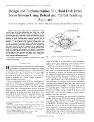
88 B. M. CHEN, A. SABERIANDP. SANNUTInecessarily imply the recoverability of the corresponding target loop transferfunction in 5.Example 6.1.Consider a non-strictly proper system characterized byA = [ ~ ~ l B=C=D=[~ ~ lwhich is invertible with two unstable invariant zeros at S=1 and S= 2. Let thetarget loop Lt(s) and target sensitivity function 5t(s) be specified byF = [ ~ ~ lNow consider a subspace 5 which is a span of the vector,Let0.7071VS =[ 0.7071 ] .10 -9K(a) = [ 4 -3 ] .Then the plots in Fig. 6.1 clearly show that amaAEs(jw) ]=0, and hence 5t(s) isexactly recoverable in the subspace 5. On the other hand, amax[E(jw)PS] isnonzero which implies that Lt(s) is not recoverable in 5.The followingobservation pertains to the case when 5=gllm.Observation 6.1. If 5=gllm, then 5t(s)=[lm+L,(s)]-1 is exactly recoverablein 5, if and only if the corresponding target loop transfer function Lt(s) isexactly recoverable in 5. Similarly, if 5=gllm, then 5t(s) is asymptoticallyrecoverable in 5, if and only if Lt(s) is asymptotically recoverable in 5.1------- "', , ,\\\\\\ amaAE(jw)PS]\ amax[ES(j w) ], ,,,,01 --'-'- .-. _.-. _._'::::.~--_.__.__._.0.8

Loop transfer recovery, Part I-Analysis 89Proof. 5=£7lm implies that PS=/m and MS(s)=M(s). Hence, the resultfollows from Lemmas 6.1 and 4.1.In view of the results of Observation 6.1, for the case when 5 =£7lm, therecoverability of any sensitivity function in £7lmdoes indeed imply the recoverabilityof the corresponding target loop transfer function in £7lm.This impliesthen that when 5 =£7lm,Definitions 6.1 to 6.5 are equivalent to the Definitions.2.1 to 2.5 given earlier. On the other hand, Definitions 6.1 to 6.5 generalize theconcept of recovery to a subspace and thus enable us to reanalyze all the resultsof the previous two sections to cover recovery in a given subs pace 5.To proceed with the recovery analysis, let VS be a matrix whose columnsform an orthogonal basis of 5E£7lm. Assume that the columns of VS are scaled sothat the norm of each column is unity. Let ps = VS(VS) I be the unique orthogonalprojection matrix onto 5. Then, define an auxiliary system ~s characterized bythe quadruple (A, BVs, C, DVS). Now treating ~s as the given system, one canrediscuss here mutatis mutandis all the results of Sees. 4 and 5. In particular, wehave the following theorems.Theorem 6.1. Consider a given system ~ characterized by a matrix quadruple(A, B, C, D), which is not necessarily of minimum phase and which is notnecessarily left invertible. Let VS be a matrix whose columns form an orthogonalbasis of a given subspace 5E£7lm. Then any admissible sensitivity function 5/s)of ~, Le., 5t(s) E S (~) is asymptotically recoverable in 5 if the auxiliary system~S is left invertible and of minimum phase.Proof.It is obvious.Theorem 6.1 is concerned with the recovery analysis when F is arbitrary orunknown. As in Sec. 5, one can formulate the recovery conditionsfor a knownFas follows.Theorem 6.2. Consider a given system ~ characterized by a matrix quadruple(A, B, C, D), which is not necessarily of minimumphase and which is notnecessarily left invertible. Let VSbe a matrix whose columnsform an orthogonalbasis of a given subspace 5E£7lm.Then an admissible sensitivity function 5t(s)of ~, i.e., 5t(s)ES(~), is exactly recoverable in 5 by means of a full orderobserver based controller, if and onlyif 5-(A, BVs, C, DVS)!;;Ker(F). That is,SER(~, 5)= {5t(S)ES(~): 5-(A, BVs, C, DVS)!;;Ker(F)}.Proof. The proof is a consequence of Theorem 5.1.In what follows, we give a necessary and sufficient condition under whichSER(~, 5) is non-empty for the given subspace 5E£7lm.We have the followingtheorem.Theorem 6.3. Consider a given system ~ characterized by a matrix quadruple(A, B, C, D), which is not necessarily of minimumphase and which is notnecessarily left invertible. Let VSbe a matrix whose columnsform an orthogonalbasis of a given subspace 5E£7lm. Let [;se be any full rank matrix such thatKer([;se)=5-(A, BVs, C, DVS). Then the given system ~ has at least onetarget sensitivity function that is exactly recoverable in 5, Le., SER(~, 5) isnonempty, if and only if an auxiliary system ~se characterized by the matrixtriple (A, B, [;se)is stabilizable by a static output feedback controller.

90 B. M. CHEN, A. SABERIANDP. SANNUTIProof. The proof is a consequence of Theorem 5.2.The followingtheorem deals with asymptotic recoverability of St(s).Theorem 6.4. Consider a given system 1: characterized by a matrix quadruple(A, B, C, D), which is not necessarily of minimumphase and which is notnecessarily left invertible. Let VSbe a matrix whose columnsform an orthogonalbasis of a given subspace 5E[?Jlm.Then an admissible sensitivity function St(s)of 1:, i.e., St(s)ES(1:), is asymptotically recoverable in 5 by means of a fullorder observer based controller, if and onlyif V+(A, BVs, C, DVS)~Ker(F).That is, SR(1:, 5)= {St(s)ES(1:): V+(A, BVS, C, DVS)~Ker(F)}.Proof. The proof is a consequence of Theorem 5.3.Again, as in Theorem 6.3, we have the following theorem regardingnon-emptiness of the set SR(1:, 5).Theorem 6.5. Consider a given system 1: characterized by a matrix quadruple(A, B, C, D), which is not necessarily of minimum phase and which is notnecessarily left invertible. Let VSbe a matrix whose columns form an orthogonalbasis of a given subspace 5E[?Jlm. Let csa be any full rank matrix such thatKer(CSa)= V+(A, BVs, C, DVS). Then, the given system 1: has at least onetarget sensitivity function that is recoverable in 5, i.e., SR(1:, 5) is nonempty, ifand only if an auxiliary system 1:sa characterized by the matrix triple (A, B,csa) is stabilizable by a static output feedback controller.Proof. The proof is a consequence of Theorem 5.4.An important aspect that arises when one is interested in recovery analysisin a subspace is to determine the maximumpossible dimensionof a recoverablesubspace 5. In this regard, our goal in what follows, as in Saberi et al. (1991 a),is to prove that whatever may be the given target loop transfer function andwhatever may be the number of unstable invariant zeros, there exists at leastone m -1 dimensional subspace 5 of [?Jlmwhich is always recoverable providedthat the given system is left invertible. To prove this, for simplicity ofpresentation, we willmake a technical assumption that all the unstable invariantzeros of 1:have geometric multiplicityequal to unity. Wenext state two lemmaswhich lead to the intended result.Lemma 6.2. Let the given system 1: be left invertible and let z, x and Wberespectively an invariant zero, the associated right state and input zerodirections of 1:. Then we have the followingproperties.1. The auxiliary system 1:Sis left invertible.2. Every invariant zero and the associated right state zero direction of 1:Sarealso the invariant zero and the associated right state zero direction of 1:.3. z and x are respectively an invariant zero and the associated right state zerodirection of 1:s,if and only if wE5.Proof. See Appendix I.Now let Zi, Xi and Wi, i= 1,''', n;i, be respectively an unstable invariant zeroand the associated right state and input zero directions of the given system 1:.Since 1: is assumed to be stabilizable and detectable, we have Wi:;i:Ofor alli=l,"',n;i. Because if Wi=O, then by definition,

Loop transfer recovery, Part I-Analysis 91(zJn-A)Xj = BWj = 0, CXj + DWj = CXj = O.This implies that Zj is an output decoupling zero of 2:. But this contradictsdetectability of 2: as ZjE C +. Next let us define for each i = 1,. .. ,n:,theNj = Ker[wi].Since Wj=,60,each Nj is an m -1 dimensional subspace. We have the followinglemma.Lemma 6.3.Proof.There exists at least one nonzero vector eE[llm such thatn+e $. Ij Nj.1=1See Saberi et al. (1991 a).Thus, in view of Lemma 6.3, there exists at least one e such thatWe have the followingtheorem.e'Wj =,60 for all i = 1, ..., n~. (6.3)Theorem 6.6. Let the given system 2: be left invertible with unstableinvariant zeros having geometric multiplicityequal to unity. Then, there existsat least one m -1 dimensionalsubspace 5 of [llmsuch that any admissibletargetsensitivity functions St(s) of 2:, i.e., St(s)ES(2:), is recoverable in S.Proof.Select e as in (6.3). Define 5 as5 = The orthogonal complement of the subspace spanned by e in [llm.Then, it is trivial to see 5 has a dimension of m-1 and that Wj$.S for alli=l,...,n~. Because if wjES, say wj=VSvjES, then e'wj=O which is acontradiction. In view of Lemma 6.2, this implies that 2:Sis left invertible and ofminimumphase. This in turn implies the results of Theorem 6.6.7. ConclusionsHere we deal with issues concerning the analysis of loop transfer recoveryproblem using full order observer based controllers for general non-strictlyproper systems. As in our earlier work, all the analysis given here is independentof the methodology by which observers are designed. There are severalfundamental results given here. Based on the structural properties of the givensystem, we decompose the recovery error between the target loop transferfunction and that which can be achieved by the observer based controllers, intothree distinct parts for any arbitrarily specified target loop transfer function.The first part of recovery error can be rendered exactly zero by an appropriatefinite eigenstructure assignment of the observer dynamic matrix, while thesecond part can be rendered arbitrarily close to zero by an appropriateasymptotically infinite eigenstructure assignment. The third part in generalcannot be rendered zero, either exactly or asymptotically, by any meansalthough there exists a multitude of ways to shape it. Such a decomposition of

92 B. M. CHEN, A. SABERIANDP. SANNUTIloop transfer function recovery mechanism helps us to discover the subspace ofthe control space in which target sensitivity and complimentary sensitivityfunctions can either exactly or asymptotically be recovered. Moreover, it helpsto formulate explicit singular value bounds on the recovery error. All thisanalysis is given for an arbitrarily specified target loop transfer function. Thus, itshows the limitations of the given system in recovering the target loop transferfunctions as a consequence of its structural properties, namely finite and infinitezero structure and invertibility. On the other hand, the next issue of our analysisconcentrates on characterizing the required necessary and sufficient conditionson the target loop transfer functions so that they are either exactly orasymptotically recoverable by means of observer based controllers for the givensystem. The conditions developed here on a target loop transfer function for itsrecoverability, turn out to be constraints on its finite and infinite zero structureas related to the corresponding structure of the given system. We next move onto find the necessary and sufficient conditions on the given system such that ithas at least one recoverable target loop. In this regard, we show that strongstabilizability of the given system is necessary for it to have at least onerecoverable target loop. Since recovery in all control loops in general is notfeasible, we concentrate next in developing the necessary and/or sufficientconditions under which either exact or asymptotic recovery of target sensitivityand complimentary sensitivity functions is possible in any specified subspace ofthe control space. This generalizes the traditional notion of LTR to coverrecoverability in a subspace. We prove next that for left invertible non-strictlyproper systems irrespective of the number of unstable invariant zeros andirrespective of the nature of the target loop transfer function, there exists atleast one m -1 dimensional subspace of m dimensional control space, in whichthe target sensitivity and complimentary sensitivity functions can always berecovered by an appropriate design of the controller. Inherent in all the issuesdiscussed here is the characterization of the resulting controller eigenvalues andpossible pole zero cancellations. Such an investigation is important in view of thefact, controller eigenvalues become the invariant zeros of the closed-loopsystem and thus affect the performance with respect to command following andother design objectives.To summarize, the analysis presented here adds a considerable amount offlexibility to the process of design and helps a designer to set meaningful goals atthe onset of design. In other words, although the actual physical tasks of firstdesigning a target loop and then designing an observer based controller areseparable, one can link these two tasks philosophically by knowing ahead what isfeasible and how. In a sequel to this paper, we will present design methodologieswhich are capable of utilizing the complete freedom a design can have as isdiscovered here.ReferencesAthans, M. (1986). A Tutorial on LQG/LTRmethods. Proceedingsof American ControlConference,Seattle, Washington, 1289-1296.Chen, B.M., A. Saberi., P. Bingulacand P. Sannuti (1990). Loop transfer recovery fornon-strictly proper plants. Control-Theory and Advanced Technology(C-TAT), 6, 4,573-594.

Loop transfer recovery, Part I-Analysis 93Chen, B.M., A. Saberi and P. Sannuti (1991 a). A new stable compensator design forexact and approximate loop transfer recovery. Automatica, 27, 2, 257-280.Chen, B.M., A. Saberi and P. Sannuti (1991 b). Necessary and sufficientconditionsfor anonminimumphase plant to have a recoverable target loop-A stable compensatordesign for LTR.Proc. 30th IEEE Conferenceon Decisionand Control, Brighton, U.K.;to appear in Automatica.Chen, B.M., A. Saberi and P. Sannuti (1992). Loop transfer recovery for generalnonminimumphase non-strictly proper systems, Part 2-Design. Control-TheoryandAdvanced Technology(C-TAT), this issue.Doyle, ].C. and G. Stein (1979). Robustness with observers. IEEE Trans. AutomaticControl, AC-24, 4, 607-611.Doyle, ]. C. and G. Stein (1981). Multivariablefeedback design: Concepts for a classical!modern synthesis. IEEE Trans. Automatic Control, AC-26, 1, 4-16.Goodman, G.C. (1984). The LQG/LTR method and discrete-time control systems.Report No. LIDS-TH-1392,M.LT., MA.Kwakernaak, H. (1969). Optimallow sensitivity linear feedback systems. Automatica, 5,2, 279-285.Matson, C.L. and P.S. Maybeck (1991). On an assumed convergence result in theLQG/LTRtechnique. IEEE Trans. Automatic Control, AC-36, 1, 123-125.Moore, B.C. (1976). On the flexibilityoffered by state feedback in multivariablesystemsbeyond closed loopeigenvalue assignment. IEEE Trans. Automatic Control, AC-21, 5,689-692.Niemann, H.H. and O. Jannerup (1990). An analysis of pole/zero cancellationin LTRbasedfeedback design. Proceedingsof 1990American Control Conference,San Diego,California,848-853.Niemann, H.H., P. Sogaard-Andersen and]. Stoustrup (1991). Loop transfer recovery:Analysis and design for general observer architecture. Int. ]. Control, 53, 5, 1177-1203.Ridgely, D.B. and S.S. Banda(1986). Introductionto robust multivariablecontrol. ReportNo. AFWAL-TR-85-3102,Flight Dynamics Laboratories, Air Force Systems Command,Wright-Patterson Air Force Base, Ohio.Rosenbrock, H.H. (1970). State-Spaceand Multivariable Theory.John-Wiley,N.Y.Saberi, A., B.M. Chen and P. Sannuti (1991 a). Theory of LTR for nonminimumphasesystems, recoverable target loops, recovery in a subspace-Part 1: Analysis. Int. ].Control, 53, 5, 1067-1115.Saberi, A., Chen, B.M. and P. Sannuti (1991 b). Theory of LTR for nonminimumphasesystems, recoverable target loops, recovery in a subspace-Part 2: Design. Int. ].Control, 53, 5, 1117-1160.Saberi, A. and P. Sannuti (1990 a). Observer design for loop transfer recovery and foruncertain dynamicalsystems. IEEE Trans. Automatic Control, AC-35, 8, 878-897.Saberi, A. and P. Sannuti(1990b). Squaringdown of non-strictly proper systems. Int.].Control, 51, 3, 621-629.Sannuti, P. and A. Saberi (1987). A special coordinate basis of multivariable linearsystems-Finite and infinite zero structure, squaring down and decoupling. Int. ].Control, 45, 5, 1655-1704.Scherer, C. (1992). H ",-optimizationwithout assumptions on finite or infinite zeros.SIAM]. Control & Optimization, 30, 1, 143-166.Shaked, U. (1977). The admissibility of desired transfer-function matrices. Int. ].Control, 25, 5,213-228.Sogaard-Andersen, P. and H.H. Niemann (1989). Trade-offs in LTR-based feedbackdesign. Proceedingsof 1989 American Control Conference, Pittsburgh, Pennsylvania,922-928.Sogaard-Andersen, P. (1989). Loop transfer recovery-An eigen-structure interpretation.Control-Theory and Advanced Technology(C-TAT), 5, 3, 351-365.

94 B. M. CHEN, A. SABERIANDP. SANNUTISogaard-Andersen, P. (1987). An eigenspace and residual approach to transfer functionmatrix synthesis. Systems & ControlLetters, 8, 221-223.Stein, G. and M. Athans (1987). The LQG/LTRprocedure for multivariable feedbackcontrol design. IEEE Trans. Automatic Control, AC-32, 2, 105-114.Stoorvogel, A.A. (1990). The singularH2 control problem. MemorandumCOSOR 90-43,Eindhoven University of Technology; to appear in Automatica.Vidyasagar, M. (1985). ControlSystemSynthesis:A FactorizationApproach.MIT Press,Cambridge, MA.Zhang, Z. and J,S. Freudenberg (1990). Loop transfer recovery for nonminimumphaseplants. IEEE Trans. Automatic Control, AC-35, 5, 547-553.Hence,Appendix A: Proof of Lemma 4.1We have the following obvious reductions:Lo(s) = C (s)P(s)= F[cJ>-l+BF+KC-KDF]-lK[CcJ>B+D]= F[In+ (cJ>-1+KC)-l(B - KD)F]-l( cJ>-1+KC)-lK[CcJ>B +D]= [In +F( cJ>-1+KC)-l(B - KD) ]-IF( cJ>-1+KC)-lK[CcJ>B + D]= [Im+M(s) ]-l[FcJ>B-F( cJ>-1+KC)-l(B -KD)]= [Im+M(s)]-l[FcJ>B-M(s)].E(s) = Lt(s) - Lo(s)= M(s)[Im+M(s)]-l(Im+FcJ>B).Appendix B: Proof of Lemma 4.2Let Ai and Vi be an eigenvalue and the corresponding left eigenvector ofA - KC for any gainK. To show that there are at most n;;+ nbleft eigenvectorsof A - KC for any gain K such that the corresponding AiE C- and thatVf(B -KD) =0, consider the dual system 2:dcharacterized by (Ad, Bd' Cd, Dd)whereAd = A', Bd = C', Cd = B', Dd = D'.Let Vd be the subspace of all right eigenvectors Vd of (Ad-BdKd) for some Kdsuch that (Cd-DdKd)Vd=O. Observe that Vd is a stable (Ad, Bd)-invariantsubspace. Furthermore, Vd is in the kernel of (Cd- DdKd)' Hence, Vd is asubset of V-(Ad, Bd, Cd, Dd). The largest possible dimension of V-(Ad, Bd,Cd, D d) is n;;+ nb' Hence, there are at most n;;+ nb left eigenvectors of A - K Cfor any gain K such that the corresponding AiE C- and that vf (B - KD) = 0.We now proceed to determine the necessary gain K to assign such eigenvalues.Without loss of generality we can assume that the given system isrepresented by the s. c.b as given in Theorem 3. 1. Then, consider a gain K ofthe form,

Loop transfer recovery, Part l-Analysis 95K=BoaBtaBObBoeBotL~t0Lbt00L~b0Kbb00where Kbb is selected such that A(Abb-KbbCb) are in C-. Let Va- and Vbrespectively be any left eigenvectors of A~a and Abb- KbbCb. It can easily beverified that A(A~a) and A(Abb-KbbCb) are among the eigenvalues of A-KCand that [V~-, 0, 0, 0, ot and [0, 0, V:, 0, ot are the associated lefteigenvectors of A-KC. Furthermore, it is easy to verify thatand similarly[V~-, 0, 0, 0, O](B-KD) = [V~-, 0, 0, 0, 0][0, 0, V:, 0, O](B-KD) = O.0000000000 0 Be0 Bt 0= 0Finally, in view of the properties of s.c.b, it is straightforward to see that suchvectors [V~-, 0, 0, 0, ot and [0, 0, V:, 0, ot respectively span thesubspacesx~andxb' Moreover, x~spans V*(A, B, C, D)/V+(A, B, C, D) andhence the result.Appendix C: Proof of Theorem 4.1Expression (4.13) followsdirectly from the definitionof K*(1:, a). To prove(4.14) and (4.15), let us consider the following.From (4.1), we haveand henceE(s, a) = FcJJB- C(s, a)P(s)= M(s, a)[I+M(s, a)]-l(l+FcJJB),I + C (s, a)P(s) = I + FcJJB- E(s, a)= I + FcJJB- M(s, a)[I+M(s, a)]-l(l+FcJJB)= [I+M(s, a)]-l(l+FcJJB).Thus, we obtainSo(s, a) = St(s)[I + M(s, a)](C.1)andTo(s, a) = Tt(s) - St(s)M(s, a). (C.2)

96 B. M. CHEN, A. SABERIANDP. SANNUTIIt is simple to see that (4.14) and (4.15) followfrom the definitionof K*(~, a).We now proceed to show (4.16) and (4.17). Applyingsingular value inequalitiesto (C.l), we have for each i = 1," " m,and thus,aj[So(jw, a)] :$ aj[St(jw)] + amax[St(jw)M(jw, a)),aj[So(jw, a)] - aj[S/jw)] :$ amax[S/jw)]amax[M(jw, a)). (C.3)Now rewriting(C.1) as,St(s) = So(s, a) - St(s)M(s, a),we have for each i = 1, .. . , maj[S/jw)] - aj[So(jw, a)]:$ amax[StUw)]amax[M(jw, a)]. (C.4)Then, in view of (C.3) and (C.4), we getIaj[So(jw, a)] - aj[St(jw)] Iamax[St(jw)]:$amax[M(jw, a)].Next using singular value inequalities and proceeding as above, we getI(Tj[To(jw, a)] - aj[Tt(jw)] I :$ amaAM(jw, a)).amax[StUw)]Then, (4.16) and (4.17) follow trivially. This completes the proof of Theorem4.1.Appendix D: Proof of Lemma 4.4For economy of notations, we drop the dependency on a throughout thisproof. Noting from Lemma 4.1 thatwe obtain,E(s) 4 Lt(s) - C(s)P(s) = M(s)[Im+M(s)]-l[Im+Lt(s)],C(s)P(s) = L/s) -M(s) [Im+M(s)]-l[Im+Lt(s)]= [Im+M(s)]-l[Lt(s)-M(s)).The above expression facilitates the interpretation of C(s)P(s) in terms of ablock diagram given below (Fig. D.1).In view of the above block diagram, it is straightforward to write astate-space realization of C(s)P(s) as

Loop transfer recovery, Part I-Analysis 97u -u+Fig. D.l.Interpretation of C(s)P(s).j-:.. A 0B[] [ ]~ (B-K~)F A-KC-BF+KDF X + B-KD u,-u = [F, -F]x.Let Abe an eigenvalue of A - KC and the corresponding left eigenvector V besuch that VH(B-KD)=O. It is simple then to verify that-andH AI-A 0[0, V] [ -(B-KD)F AI-A+KC+(B-KD)F ] = 0H B[0, V ][B-KD ] = O.This shows that A is an input decoupling zero of C(s)P(s)follows.and thus the resultAppendix E: Proof of Theorem 5.1Consider an auxiliary system characterizedbyl:au: .!i = A'x + C'u + F'w,z=B'x+D'u.(E.1)Then, with a state feedback lawu = -K'x,the closed-loop transfer function from w to z, denoted here by T~::'(s), is simplyT~::'(s)= M'(s).Hence, the problem of finding an observer gain matrix such that A - KC isasymptotically stable and that M(s)=O is equivalent to the well-known disturbancedecoupling problem with internal stability when the plant considered is l:auas given in (E.1). Then, it follows from Stoorvogel (1990) that the abovedisturbance decoupling problem with internal stability is solvable, if and only ifS-(A, B, C, D)5;;Ker(F).

98 B. M. CHEN, A. SABERIANDP. SANNUTIAppendix F: Proof of Theorem 5.2Without loss of generality we assume that the given system ~ is in the formof s.c. b as in Theorem 3.1. Now in view of Theorem 5.1, an exactly recoverableLt(s)=FCPB must satisfy S-(A, B, C, D)~Ker(F). This implies that Lt(s) isrecoverable, if and only if F is of the form,F =[F~I 0 FbI 0F~2 0 F b2 0 ~ l(F.1)Thus, the fact that the given system has at least one exactly recoverable targetloop is equivalent to the existence of some appropriate matrices F~I, FbI, F~2and F b2such that A - BF is asymptoticallystable.Next, inviewofthe factthatX; EihcEBxfspansS-(A, B, C, D), we note that CERas defined in Theorem 5.2is of the form,CER= r[ 1(/000Inb00 ~ lwhere r is any nonsingular matrix of dimension (n - ne- nf) x (n - ne- nf). It isnow trivial to verify that the existence ofa matrixF of the form in (F.1) such thatA - BF is asymptoticallystable, is equivalentto the existenceof a matrixG ofdimension m x(n-ne- nf) such that A -BGCER is asymptotically stable. This issimply due to the fact that GCERhas the same structure as F in (F.1). Thiscompletes the proof of Theorem 5.2.Appendix G: Proof of Corollary 5.4It is well known that any stabilizable and detectable system ~ can bestabilized by using an observer based controller. We next prove that ~ isstrongly stabilizable whenever it has at least one asymptotically recoverabletarget loop transfer function Lt(s) =FCPB. The fact that there exists at least oneasymptotically recoverable L/s) implies that there exists a gain F such thatA-BF is asymptotically stable and V+(A, B, C, D)~Ker(F). Moreover,asymptotic recoverability of Lt(s) implies that there exists an observer gain,K(a), such that A-K(a)C is asymptotically stable andM(s, a) = F[cp-I+K(a)C]-l[B-K(a)D] ~ 0pointwise in s as a ~ 00. (G.1)Next, we examine the eigenvalues of the full order observer based controller.view of Eqs. (4.22) and (G.1), we haveIndet[sIn -A + K(a)C + BF - K(a)DF] ~ljJo(s)ljJoo(s)ljJe(s),as a~oo, where the roots of ljJo(s)ljJoo(s)ljJe(s)=Oare the eigenvalues ofA-K(a)C. Thus, the full order observer based controller is open-loop stablefor sufficiently large a. We conclude then that the given system ~ is stronglystabilizable as it can be stabilized by an open-loop stable controller.

Hence,Let us recall thatLoop transfer recovery, Part l-Analysis 99Appendix H: Proof of Lemma 6.1E(s) = Lt(s) - Lo(s)= F

100 B. M. CHEN, A. SABERIANDP. SANNUTIThis proves the second property of the lemma. Let us next prove the sufficiencypart of Property 3. Let w= VSv, thenimplies that[ ZInC A-: ][ ~ ]= 0[ zInC A-BVSDVS][xv] = O.As IS is left invertible, the above implies that z and x are an invariant zero andthe associated right state zero direction of IS. To prove necessity, assume thatz and x are an invariant zero and the associated right state zero direction of IS.Then, there exists a wSsuch that(zIn-A)x = BVswS, Cx + DVsws = O.In view of this and by the definition of z, x and w, we haveBVswS = Bw,DVswS = Dw.Since [B', D']' is of full rank, it implies then that wE S.. '. '. '.'. '.'. ,.'. .'...'.'.'.' .,Ben M. Chen see p.35 in this issue.Ali Saberi see p.35 in this issue.Peddapullaiah Sannuti was born in Rajupalem,Proddatur (Taluk), India. He receivedthe B.E. degree (with honors) inelectrical engineering from the College ofEngineering, Anantapur, India, in 1963, theM. Tech. degree in control systems engineeringfrom the Indian Institute of Technology,Kharagpur, India, in 1965, and thePh.D. degree in electrical engineering fromthe University of Illinois, Urbana-Champaign,in 1968.From 1965 to 1968, he was first aTeaching Assistant and then a ResearchAssistant in the Department of ElectricalEngineering and the Coordinated ScienceLaboratory, University of Illinois. Since1968 he has been with the Department ofElectrical Engineering, Rutgers University, Piscataway, N.]., where he iscurrently a Professor. His research interests include singular perturbationtheory, computational methods, and communication theory.