Learning the Delaunay Triangulation of Landmarks From a ... - LaValle

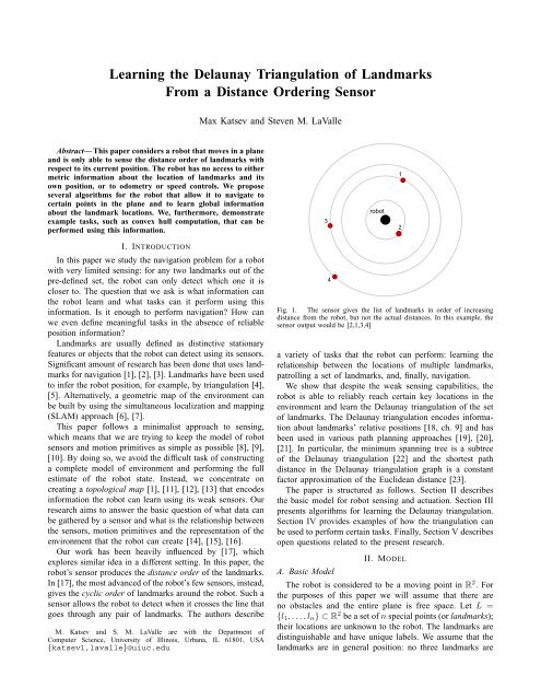
Learning the Delaunay Triangulation of LandmarksFrom a Distance Ordering SensorMax Katsev and Steven M. LaValleAbstract— This paper considers a robot that moves in a planeand is only able to sense the distance order of landmarks withrespect to its current position. The robot has no access to eithermetric information about the location of landmarks and itsown position, or to odometry or speed controls. We proposeseveral algorithms for the robot that allow it to navigate tocertain points in the plane and to learn global informationabout the landmark locations. We, furthermore, demonstrateexample tasks, such as convex hull computation, that can beperformed using this information.I. INTRODUCTIONIn this paper we study the navigation problem for a robotwith very limited sensing: for any two landmarks out of thepre-defined set, the robot can only detect which one it iscloser to. The question that we ask is what information canthe robot learn and what tasks can it perform using thisinformation. Is it enough to perform navigation? How canwe even define meaningful tasks in the absence of reliableposition information?Landmarks are usually defined as distinctive stationaryfeatures or objects that the robot can detect using its sensors.Significant amount of research has been done that uses landmarksfor navigation [1], [2], [3]. Landmarks have been usedto infer the robot position, for example, by triangulation [4],[5]. Alternatively, a geometric map of the environment canbe built by using the simultaneous localization and mapping(SLAM) approach [6], [7].This paper follows a minimalist approach to sensing,which means that we are trying to keep the model of robotsensors and motion primitives as simple as possible [8], [9],[10]. By doing so, we avoid the difficult task of constructinga complete model of environment and performing the fullestimate of the robot state. Instead, we concentrate oncreating a topological map [1], [11], [12], [13] that encodesinformation the robot can learn using its weak sensors. Ourresearch aims to answer the basic question of what data canbe gathered by a sensor and what is the relationship betweenthe sensors, motion primitives and the representation of theenvironment that the robot can create [14], [15], [16].Our work has been heavily influenced by [17], whichexplores similar idea in a different setting. In this paper, therobot’s sensor produces the distance order of the landmarks.In [17], the most advanced of the robot’s few sensors, instead,gives the cyclic order of landmarks around the robot. Such asensor allows the robot to detect when it crosses the line thatgoes through any pair of landmarks. The authors describeM. Katsev and S. M. LaValle are with the Department ofComputer Science, University of Illinois, Urbana, IL 61801, USA{katsev1,lavalle}@uiuc.eduFig. 1. The sensor gives the list of landmarks in order of increasingdistance from the robot, but not the actual distances. In this example, thesensor output would be [2,1,3,4]a variety of tasks that the robot can perform: learning therelationship between the locations of multiple landmarks,patrolling a set of landmarks, and, finally, navigation.We show that despite the weak sensing capabilities, therobot is able to reliably reach certain key locations in theenvironment and learn the Delaunay triangulation of the setof landmarks. The Delaunay triangulation encodes informationabout landmarks’ relative positions [18, ch. 9] and hasbeen used in various path planning approaches [19], [20],[21]. In particular, the minimum spanning tree is a subtreeof the Delaunay triangulation [22] and the shortest pathdistance in the Delaunay triangulation graph is a constantfactor approximation of the Euclidean distance [23].The paper is structured as follows. Section II describesthe basic model for robot sensing and actuation. Section IIIpresents algorithms for learning the Delaunay triangulation.Section IV provides examples of how the triangulation canbe used to perform certain tasks. Finally, Section V describesopen questions related to the present research.A. Basic ModelII. MODELThe robot is considered to be a moving point in R 2 . Forthe purposes of this paper we will assume that there areno obstacles and the entire plane is free space. Let L ={l 1 ,...,l n } ⊂ R 2 be a set ofnspecial points (or landmarks);their locations are unknown to the robot. The landmarks aredistinguishable and have unique labels. We assume that thelandmarks are in general position: no three landmarks are

(a) Projections of both direction fields onthe bisector have the same direction. Therobot will move in that direction until itreaches point AFig. 2. Perpendicular bisectors split the environment into polygonalpreimages. Each preimage can be uniquely identified by the sensor outputwhen the robot is inside the region. Some preimage labels are omitted forclaritycollinear, no four landmarks are cocircular, and no landmarkis equidistant from two other landmarks.Let r ∈ R 2 be the current robot position. The state spacefor the robot is defined as(b) Projections of both direction fields on thebisector have opposite directions. The robotbehavior is not clearly defined.X = R 2 ×E,in which E ⊂ R 2n is a set of all possible landmarkconfigurations.The robot is equipped with a distance ordering sensorthat returns the sequence of landmark labels ordered by thedistance relative to the current robot position in ascendingorder (see Fig. 1) and additional information about landmarksthat are equidistant from the robot. Such a sensor can beimplemented, for example, by comparing the strength ofradio signals transmitted by the landmarks.The robot is able to execute two motion primitives:TOWARD(l) and AWAY(l). TOWARD(l) results in the robotmoving in a straight line in the direction of the landmarklabeled l, whereas AWAY(l) moves the robot in the oppositedirection (AWAY(l) is undefined when the robot is at l).Additionally, TOWARD(l) terminates when the robot arrivesat l. Note that these motion primitives do not provide therobot with any information about the relationship betweendirections to multiple landmarks.B. Additional ConsiderationsThe distance ordering sensor can be defined by a sensormappingh : X → S n ×P n−1 ,in which S n is a set of all possible permutations of n distinctelements and P n−1 is the powerset of {1,...,n − 1}. Thefirst part of the output lists the landmarks in the order ofascending distance to the robot. The second part encodesgroups of landmarks with equal distances to the current robotlocation: if it contains index i, then distances to the i-thand i + 1-th closest landmarks are equal. For example, ifh(r,E) = ((l 4 ,l 2 ,l 1 ,l 3 ),{1,2}), then, in the configurationE, the distances from r to l 4 , l 2 , and l 1 are equal and smallerthan the distance to l 3 .(c) We resolve the ambiguity by introducing a sensor reaction delay(dotted curves show where the sensor output changes after the robothas crossed the bisector). The robot will move in the directioncorresponding to the larger projection of the direction field on thebisector (in the direction of point C, in this example).Fig. 3.Various robot behavior at the boundary between preimagesAlternatively, the sensor output can be encoded as a linearorder relation “closer than or equidistant to” on the set oflandmarks L that can be represented as an n×n matrix withelements ±1 that satisfies certain properties (for example,one of them is to be antisymmetric).This mapping decomposes the plane into preimages: regionsin which the sensor output is constant. For the distanceordering sensor, the preimages are polygons created by theperpendicular bisectors (simply bisectors in the future) ofpairs of the landmarks (see Fig. 2), the bisectors themselves,and the intersection points of multiple bisectors.The robot can only change its behavior when its sensorreadings change, specifically, when it crosses one of thebisectors (we assume that the robot neither controls norknows its speed; therefore, the notion of time is meaninglessin our setting). We use the term direction field to describea vector field that assigns to each point of the plane thedirection of the robot movement at that point. Due to thespecifics of the motion primitives available to the robot, thedirection field varies smoothly inside every preimage (withthe possible exception of landmark locations). However, itmight be problematic to define the robot direction on theboundary between multiple preimages (see Fig. 3).In the situation depicted in Fig. 3(a), it is reasonable

to conclude that the robot will continue moving along thebisector line in the general direction of the landmarks untilit reaches pointA, then stop; Fig. 3(b) is more ambiguous. Toresolve this issue, we will refer to a somewhat different robotmodel in which the distance ordering sensor has boundedpolling rate. Effectively, this means that there is a (bounded)delay between the robot crossing the bisector line and thesensor reading being updated. As a result, the actual robottrajectory will look similar to Fig. 3(c): in general, the robotdirection is determined by the direction field that has a largerprojection on the bisector. In the example of Fig. 3(c), therobot moves along the bisector towards point C. This allowsus to make the following statement:Proposition 1 (Extending the direction field to the preimageboundaries). Let q be a point on the bisector line thatseparates preimages P 1 and P 2 . Let d 1 and d 2 be continuousextensions to q of the robot direction field defined on P 1 andP 2 , correspondingly.1) If both d 1 and d 2 are outward-pointing for P 1 and P 2 ,then the robot direction atq is defined by the projectionof d 1 +d 2 on the bisector line.2) If d 1 is outward-pointing and d 2 is inward-pointing,then the robot direction at q is defined by d 1 .3) If both d 1 and d 2 are inward-pointing, then the robotdirection at q is undefined.It is worth remembering that the speed of the robot is nottaken into account, so the norm of the direction vector isirrelevant.III. LEARNING THE DELAUNAY TRIANGULATIONThe following notation will be used in this section:• d : R 2 × R 2 → [0,∞) is the distance function on theplane;• LAST(r) is the most distant landmark (last in the sensoroutput), when the robot is at r, defined byLAST(r) = argmaxl∈L d(r,l).A. Distinguishing Acute, Obtuse and Right AnglesThe first task the robot is able to perform is to gather someinformation about the angle formed by three landmarks. Thealgorithm 1 is very simple:Algorithm 1. (Identifying the type of an angle ∠ABC)Description. The robot executes TOWARD(A), thenTOWARD(C). The robot stops when A and C switch placesin the distance ordering. If B is the most distant of thethree landmarks, then ∠ABC < π 2; if B is the closest, then∠ABC > π 2; finally, if all three landmarks are equidistant,then ∠ABC = π 2 .Lemma 1. Algorithm 1 is correct.Proof. It can be seen that the robot stops exactly at themidpoint of the segment AC. The result follows from simplegeometric reasoning.1 It should be noted that most of the “algorithms” of this section are notalgorithms in the classical sense of the word, but rather motion strategies thatinstruct the robot how to get to a desired location, without the knowledgeof the starting state.Fig. 4.Locating the circumcenter of an acute triangle.B. Locating the Circumcenter of Three LandmarksThe crucial part of the Delaunay triangulation algorithmis to navigate the robot to the circumcenter of three givenlandmarks. The way to accomplish this task depends on thetype of the triangle formed by those landmarks. Assume forsimplicity that A, B and C are the only three landmarks.Algorithm 2. (Reaching the circumcenter of a right triangle∆ABC)Description. The robot executes TOWARD(A), thenTOWARD(C). It stops when A and C switch places in thedistance ordering.Lemma 2. If ∠ABC = π 2, then Algorithm 2 terminates withthe robot at the circumcenter of ∆ABC.Proof. The circumcenter of a right triangle is the midpointof its hypotenuse, in this case AC.Algorithm 3. (Reaching the circumcenter of an acute triangle∆ABC)Description. The robot is continuously executingTOWARD(LAST(r)), in which r is its current position.It stops when the distances to all three landmarks A, B,and C are equal. Notice that due to the iterative nature ofthe algorithm, the robot does not reach the stopping pointperfectly, but only in the limit. We might decide that therobot stops when it arrives to the desired location withgood enough precision or when the robot fails to move anysignificant distance over an extended period of time.Lemma 3. If ∠ABC < π 2, then Algorithm 3 terminates withthe robot at the circumcenter of ∆ABC.Proof. Essentially, the robot moves in the direction oppositeto the gradient of a bounded function f(r) = d(LAST(r),r).This means that it will stop at the local minimum of f. Ifthe triangle ∆ABC is acute, then the only such minimumis the circumcenter (see Fig. 4).

Fig. 5. Locating the circumcenter of an obtuse triangle. In some parts ofbisector corresponding to BA and BC, direction fields’ projections haveopposite direction. According to Proposition 1, the final robot direction isaimed at the circumcenter.Unfortunately, the previous algorithm does not work incase of an obtuse triangle, since now the local minima of f isnot the circumcenter but the midpoint of AC. The following(less elegant) modification provides the solution.Algorithm 4. (Reaching the circumcenter of an obtusetriangle ∆ABC).Description. First, the robot travels to the midpoint of AC.After having reached it, the robot continuously executesTOWARD(LAST(r)) unless B is the closest landmark; if it is,then the robot executes AWAY(B). Similarly to the previousalgorithm, the robot stops when all three landmarks become(almost) equidistant. Fig. 5 provides the illustration.There are two potential issues with this algorithm. First,for some starting robot positions, AWAY(B) will direct therobot away from the landmarks and the circumcenter, andwill never terminate. Beginning with the midpoint of ACdeals with this, since it lies in the region in which thealgorithm always terminates. Second, the use of the first partof Proposition 1 (opposite directions) is needed to determinethe robot direction at some parts of the bisector lines,specifically the regions in which B switches to or from thefirst position in the distance ordering (see Fig. 5). However,it can be shown from geometric considerations that the robotmovement is always directed toward the circumcenter.Lemma 4. Suppose ∠ABC > π 2. Algorithm 4 terminateswith the robot at the circumcenter of ∆ABC.Proof. See Appendix.Now we can derive the final algorithm for this section:Algorithm 5. (Reaching the circumcenter of any triangle∆ABC).Description. Run Algorithm 1 for each of the vertices of∆ABC to determine the type of the triangle. If all threeangles are acute, then run Algorithm 3. If one of the anglesis obtuse, relabel the landmarks so that the obtuse anglecorresponds to vertex B and run Algorithm 4. If one of theInput: A,B,C ∈ LOutput: TRUE if ∆ABC is Delaunay, FALSE otherwisetype ← acutefor all Y in {A,B,C} doX,Z ← 2 remaining verticesTOWARD(X)repeatTOWARD(Z)until equal distance to X and Zif X is not closer than Y then(A,B,C) ← (X,Y,Z)if Y is closer than X thentype ← obtuseelsetype ← rightbreakif type = acute thenrepeat// LAST ABC (r) is the last of A, B, C in the outputTOWARD(LAST ABC (r))until equal distance to A, B, and Celse if type = obtuse thenrepeatif B is closer than A and C thenAWAY(B)elseTOWARD(LAST ABC (r))until equal distance to A, B, and Cif FIRST(r) ∈ {A,B,C} thenreturn TRUEelsereturn FALSEFig. 6.Testing the Delaunay propertyangles is right, relabel the landmarks in the same way andrun Algorithm 2.The correctness of the algorithm follows from Lemmas 1-4:Theorem 1. Algorithm 5 terminates with the robot at thecircumcenter of ∆ABC.C. Computing the Delaunay TriangulationThe Delaunay triangulation for a set of points in theplane is a triangulation such that no point is in the interiorthe circumcircle of any triangle [18]. We call a triangleABC (A,B,C ∈ L) Delaunay triangle if it has the emptycircumcircle property, i.e., its circumcircle contains no pointsof L.Algorithm 6. (Testing the Delaunay property of a triangle)Description. The robot executes Algorithm 5, while ignoringall the landmarks except A, B, and C. The triangle isDelaunay if and only if the three landmarks occur at thebeginning of the distance ordering sensor output when therobot is at the circumcenter of ∆ABC. See Fig. 6 for thepseudocode representation of the algorithm.

Lemma 5. Algorithm 6 is correct.Proof. The robot can safely ignore other landmarks in thesensor output for the first step of the algorithm, since thesensor reading for a subset of landmarks is exactly thecorresponding subsequence of the full output.Furthermore, by the general position assumption, no fourlandmarks lie on the same circle. Therefore a sensor outputat the circumcenter of ∆ABC that starts with A, B, C (inany order) implies that all other landmarks are outside of thecircumcircle and the triangle is Delaunay.The faces of a Delaunay triangulation for a set of points areexactly all Delaunay triangles formed by those points [18].Therefore, we can use the following algorithm to constructthe Delaunay triangulation of L:Algorithm 7. (Computing the Delaunay triangulation)Description. Run Algorithm 6 for all triples of landmarksfrom L. If landmarks A, B, and C form a Delaunay triangle,then edges AB, AC, and BC belong to the Delaunay graph.IV. USING THE DELAUNAY TRIANGULATIONIn this section we discuss certain tasks that can beperformed using the information gathered in the previoussection.A. Computing the Convex HullThe Delaunay triangulation of a set L encodes enoughinformation to determine the convex hull of L. Indeed, theconvex hull boundary is formed by the edges of a triangulationthat belong to exactly one triangle. The only thingleft is a trivial task of connecting edges in the correct orderto form a closed path 2 . By using appropriate data structures(e.g., red-black trees), this algorithm can be adapted to runwith O(nlogn) time complexity, provided that the list ofDelaunay triangles is precomputed in advance.Algorithm 8. (Computing the convex hull)Description. See Fig. 7 for the pseudocode implementation.Suppose M ⊂ L is a set of landmarks. The robot canconstruct the Delaunay triangulation of M by using thealgorithms described in Section III and find the convex hull.However, it does not need to execute Algorithm 7 severaltimes for different M. We can modify the algorithm to allowthe robot to remember complete sensor outputs at everycircumcenter of L. In this case, the robot would only need torun Algorithm 7 once for L in order to be able to computethe triangulation of any M ⊂ L without moving anywhere.To do that, it can simply use the existing data and ignore alllandmarks from L\M.2 Videos demonstrating the execution of Algorithm 8 (implemented insimulation) are available at http://msl.cs.uiuc.edu/˜katsev1/publications/iros11/Input: Set of landmarks LOutput: Convex hull of Ledges ← ∅, hull ← ∅for all A,B,C in L doif ISDELAUNAY(∆ABC) thenfor all e in {AB,BC,AC} doif not CONTAINS(edges,e) thenINSERT(edges,e)elseDELETE(edges,e)e ← edges[0]v ← any endpoint of eDELETE(edges,e)APPEND(hull,v)repeate ← element of edges with endpoint vv ← other endpoint of eDELETE(edges,e)APPEND(hull,v)until ISEMPTY(edges)return hullB. PatrollingFig. 7.Computing the convex hullSimilarly to [17], we define the task of patrolling a setof landmarks M ⊂ L, such that M ∩∂hull(L) = ∅, as theproblem of locating a minimal set W ⊂ L such that M ⊂ Wand M ∩∂hull(W) = ∅. The idea is that we want to find aroute for the robot that would go around M, but not too farfrom it. In this case, the robot can patrol landmarks M bynavigating the convex hull boundary of W . The followingalgorithm solves this problem.Algorithm 9.Description. Start with W = L. At every iteration try tofind l ∈ ∂hull(W) such that M ∩∂hull(W \{l}) = ∅ andreplace W by W \{l}. If no such l can be found, then Wis minimal.It is unclear whether there exists an efficient algorithm tofind the smallest set W that satisfies the requirements.V. CONCLUSIONS AND FUTURE WORKWe have analyzed the capabilities of the robot that isequipped with only one weak sensor that produces thedistance ordering of the distinguishable landmarks. We havedemonstrated that the robot can successfully reach the circumcenterof a triangle formed by any triple of landmarks.This enabled us to provide an algorithm for the robot to learnthe Delaunay triangulation of the set of landmarks L. Usingthe information obtained, the robot is able to, for example,compute the convex hull of L or patrol a subset of L.Many interesting questions remain for future research. Thesensor output is based on the Euclidean distance ordering.Can it be replaced by a more general model? For example,can the underlying distance function be non-additive or lackradial symmetry? What other tasks can be performed bythe robot using the information contained in the Delaunay

triangulation? Although the Delaunay triangulation can beused for path planning, the robot can only compare length ofintervals that have a common endpoint. Does this limitationmake the optimal planning problem impossible? Algorithmsof Section III operate only on three landmarks at time.Is there a better algorithm that will use all the landmarkssimultaneously? How can obstacles incorporated in thisproblem (we might want to distinguish between two typesof obstacles: physical obstacles that block robot movementand virtual obstacles that block sensing)?APPENDIXProof of Lemma 4. Let FIRST(r) be the closest landmark,when the robot is at r, defined byConsider the functionFIRST(r) = argminl∈L d(r,l).f(r) = d(r, LAST(r))−d(r, FIRST(r)),which returns the difference between the distances to theclosest and furthest landmarks. It is continuous by constructionand its only minimum is the circumcenter of ∆ABC,at which f(r) = 0.Suppose that the robot is executing TOWARD(LAST(r))or AWAY(FIRST(r)) inside of a region in which the correspondinggoal landmark does not change. In this case, fis non-increasing and even strictly decreasing, except forsome locations on the extensions of triangle sides beyondthe vertices. Indeed, when the robot moves directly towardLAST(r), the distance to LAST(r) decreases faster than thedistance to any other landmark, including FIRST(r), thereforef is decreasing. The only exception is when the direction toLAST(r) coincides with the direction to FIRST(r), in thiscase f stays constant. This requires the robot to be co-linearwith LAST(r) and FIRST(r) and not between them. It can beseen that it is not possible for this condition to continueindefinitely, therefore f will eventually decrease. Similarreasoning applies to the motion primitive AWAY(FIRST(r)).We conclude that there are three possible scenarios for therobot: 1) it can move infinitely far away from the landmarksusing the AWAY primitive; 2) it can get stuck, because thealgorithm would instruct it to move in the opposite directionson two sides of the bisector line; 3) it can safely reach theminimum of f, the circumcenter of ∆ABC.Cases 1 and 2 only happen in certain locations. Forexample, 2 is impossible unless the robot is co-linear with Band A, or B and C. The algorithm’s initial step is intendedto drive the robot to the “safe” starting point, from which itis guaranteed to reach the circumcenter.ACKNOWLEDGMENTSThis work is supported in part by NSF grant 0904501(IIS Robotics), NSF grant 1035345 (CNS CyberphysicalSystems), DARPA SToMP grant HR0011-05-1-0008, andMURI/ONR grant N00014-09-1-1052.REFERENCES[1] H. Bulata and M. Devy, “Incremental construction of a landmark-basedand topological model of indoor environments by a mobile robot,” inProceedings of the IEEE International Conference on Robotics andAutomation, pp. 1054–1060, 1996.[2] J.-B. Hayet, C. Esteves, M. Devy, and F. Lerasle, “Qualitative modelingof indoor environments from visual landmarks and range data,” inProceedings of the IEEE/RSJ International Conference on IntelligentRobots and System, pp. 631–636, IEEE, 2002.[3] H. Hu and D. Gu, “Landmark-based navigation of mobile robots inmanufacturing,” in Proceedings of the IEEE International Conferenceon Emerging Technologies and Factory Automation, pp. 121–128,1999.[4] M. Betke and L. Gurvits, “Mobile robot localization using landmarks,”IEEE Transactions on Robotics and Automation, vol. 13, pp. 251–263,Apr. 1997.[5] I. Shimshoni, “On mobile robot localization from landmark bearings,”IEEE Transactions on Robotics and Automation, vol. 18, pp. 971–976,Dec. 2002.[6] M. Montemerlo, S. Thrun, D. Koller, and B. Wegbreit, “FastSLAM: afactored solution to the simultaneous localization and mapping problem,”in Proceedings of the AAAI National Conference on ArtificialIntelligence, pp. 593–598, July 2002.[7] D. Fox, J. Ko, K. Konolige, B. Limketkai, D. Schulz, and B. Stewart,“Distributed Multirobot Exploration and Mapping,” Proceedings of theIEEE, vol. 94, pp. 1325–1339, July 2006.[8] M. Erdmann and M. Mason, “An exploration of sensorless manipulation,”IEEE Journal on Robotics and Automation, vol. 4, no. 4,pp. 369–379, 1988.[9] V. J. Lumelsky and A. A. Stepanov, “Path-planning strategies for apoint mobile automaton moving amidst unknown obstacles of arbitraryshape,” Algorithmica, vol. 2, pp. 403–430, Nov. 1987.[10] M. Katsev, A. Yershova, B. Tovar, R. Ghrist, and S. M. LaValle,“Mapping and Pursuit-Evasion Strategies For a Simple Wall-FollowingRobot,” IEEE Transactions on Robotics, vol. 27, pp. 113–128, Feb.2011.[11] E. Remolina and B. Kuipers, “Towards a general theory of topologicalmaps,” Artificial Intelligence, vol. 152, pp. 47–104, Jan. 2004.[12] G. Dudek, M. Jenkin, E. Milios, and D. Wilkes, “Robotic explorationas graph construction,” IEEE Transactions on Robotics and Automation,vol. 7, no. 6, pp. 859–865, 1991.[13] H. Choset and K. Nagatani, “Topological simultaneous localizationand mapping (SLAM): toward exact localization without explicitlocalization,” IEEE Transactions on Robotics and Automation, vol. 17,pp. 125–137, Apr. 2001.[14] M. Blum and D. Kozen, “On the power of the compass (or, whymazes are easier to search than graphs),” in 19th Annual Symposiumon Foundations of Computer Science, pp. 132–142, IEEE, Oct. 1978.[15] B. R. Donald, “On information invariants in robotics,” ArtificialIntelligence, vol. 72, pp. 217–304, Jan. 1995.[16] M. Erdmann, “Understanding Action and Sensing by DesigningAction-Based Sensors,” The International Journal of Robotics Research,vol. 14, pp. 483–509, Oct. 1995.[17] B. Tovar, L. Freda, and S. M. LaValle, “Learning CombinatorialMap Information from Permutations of Landmarks,” The InternationalJournal of Robotics Research, Oct. 2010.[18] M. de Berg, O. Cheong, M. van Kreveld, and M. Overmars, ComputationalGeometry: Algorithms and Applications. Springer, 2008.[19] J. Chen, C. Luo, M. Krishnan, M. Paulik, and Y. Tang, “An enhanceddynamic Delaunay triangulation-based path planning algorithm forautonomous mobile robot navigation,” in Intelligent Robots and ComputerVision XXVII: Algorithms and Technique, 2010.[20] F. Gong and X. Wang, “Robot Path-Planning Based on TriangulationTracing,” in International Symposium on Intelligent Information TechnologyApplication, pp. 713–716, Dec. 2008.[21] M. Kallmann, “Path planning in triangulations,” IJCAI Workshop onReasoning, Representation, and Learning in Computer Games, 2005.[22] J. Jaromczyk and G. Toussaint, “Relative neighborhood graphs andtheir relatives,” Proceedings of the IEEE, vol. 80, no. 9, pp. 1502–1517, 1992.[23] F. Dehne, J. Sack, N. Santoro, J. Keil, and C. Gutwin, The Delaunaytriangulation closely approximates the complete Euclidean graph,pp. 47–56. Lecture Notes in Computer Science, Springer Berlin /Heidelberg, 1989.